Fluid Inertia Damping Effects on Dynamic Engine Response · PDF fileassistance in developing...
70
Fluid Inertia Damping Effects on Dynamic Engine Response by Timothy Leung A thesis submitted in conformity with the requirements for the degree of Masters of Applied Science Graduate Department of Mechanical and Industrial Engineering University of Toronto © Copyright by Tim Leung 2014
Transcript of Fluid Inertia Damping Effects on Dynamic Engine Response · PDF fileassistance in developing...

Fluid Inertia Damping Effects on Dynamic Engine Response
by
Timothy Leung
A thesis submitted in conformity with the requirements for the degree of Masters of Applied Science
Graduate Department of Mechanical and Industrial Engineering University of Toronto
© Copyright by Tim Leung 2014

ii
Fluid Inertia Damping Effects on Dynamic Engine Response
Timothy Leung
Masters of Applied Science
Graduate Department of Mechanical and Industrial Engineering
University of Toronto
2014
Abstract
Current trends in engine development are moving towards higher specific power (high rotor
speed) and lower weight to improve the fuel efficiency of aircraft. Unfortunately, this has the
adverse effect of increasing the level of engine vibrations – higher specific power results in
larger unbalanced loads while lower weight reduces the structural stiffness. To reduce the effects
of engine vibration, squeeze film dampers (SFDs) are used to add damping to the structure.
SFDs are commonly modelled using the Reynolds equation, which assumes inertial effects have
negligible impact on the damper forces. However, this assumption is not true at the higher
operating speeds of current engine designs. This thesis compares different models that include
the effect of inertia on damper forces. The models are implemented into rotor systems
representative of current engine designs and conclusions are drawn as to the significance of
inertia effects on engine response.

iii
Acknowledgments
I would like to thank Prof. Kamran Behdinan for his continuous help and guidance throughout
this project.
I would also like to thank the technical staff at Pratt and Whitney Canada for their assistance and
support for the completion of this thesis. In particular, I would like to thank Dennis Chan for his
assistance in developing the topic of this thesis and Dave Beamish for his assistance with the
finite difference solution of the Reynolds equation.
Finally I would like to thank my family for all their love and support.

iv
Table of Contents
Acknowledgments .......................................................................................................................... iii
Table of Contents ........................................................................................................................... iv
List of Tables ................................................................................................................................. vi
List of Figures ............................................................................................................................... vii
Nomenclature ................................................................................................................................. ix
Chapter 1 – Introduction ................................................................................................................. 1
1.1 Outline of Research ............................................................................................................. 4
1.2 Summary of Thesis Structure .............................................................................................. 4
Chapter 2 – Literature Review ........................................................................................................ 5
Chapter 3 – Rotordynamics .......................................................................................................... 10
3.1 Governing Equations for Rotor Systems......................................................................... 10
3.2 Critical Speeds ................................................................................................................ 12
Chapter 4 – Squeeze Film Dampers (basic features) .................................................................... 13
4.1 Analytical Solutions to the Reynolds Equation ................................................................ 16
4.1.1 Short Bearing Assumption (SBA) ........................................................................ 16
4.1.2 Long Bearing Assumption (LBA) ........................................................................ 18
4.2 Lubricant Cavitation ......................................................................................................... 19
4.3 Finite Difference Solution of Reynolds Equation ............................................................. 19
4.4 Rotordynamic Force Coefficients ..................................................................................... 21
Chapter 5 – Squeeze Film Dampers (inertial effects) ................................................................... 22
5.1 Bulk-Flow Model .............................................................................................................. 22
5.2 Temporal Inertia Effects ................................................................................................... 22
5.2.1 Temporal Force Coefficients ................................................................................ 23
5.2.2 Modified Reynolds Equation ................................................................................ 25

v
5.3 Convective Inertia Effects ................................................................................................. 26
Chapter 6 – Comparison of Inertial Damper Models .................................................................... 31
6.1 Bearing Geometry ............................................................................................................. 31
6.2 Operating Conditions ........................................................................................................ 32
6.3 Bearing Models ................................................................................................................. 32
6.4 Comparison of Damper Forces ......................................................................................... 32
Chapter 7 – Transient Response of a Rotor System ..................................................................... 38
7.1 Solution Methodology ...................................................................................................... 38
7.2 Model Assumptions .......................................................................................................... 39
7.2.1 Rotor Simulation ................................................................................................... 39
7.2.2 Temporal Force Coefficients ................................................................................ 39
7.2.3 Convective Force Coefficients .............................................................................. 39
7.3 Rotor and Bearing Models ................................................................................................ 39
7.3.1 Low Pressure (LP) Rotor ...................................................................................... 40
7.3.2 High Pressure (HP) Rotor ..................................................................................... 46
Chapter 8 – Conclusions ............................................................................................................... 52
8.1 Recommendations for Future Work ................................................................................... 53
References ..................................................................................................................................... 54
Appendices .................................................................................................................................... 58
vi
List of Tables
Table 1 - Significance of Inertia Effects for Typical Lubricants ................................................... 3
Table 2 - SFD Parameters ............................................................................................................. 31
Table 3 - Rotor Material Properties .............................................................................................. 39
Table 4 - LP Rotor Critical Speeds ............................................................................................... 42
Table 5 - LP Rotor SFD Parameters ............................................................................................. 42
Table 6 - HP Rotor Critical Speeds ............................................................................................... 48
Table 7 - HP Rotor SFD Parameters ............................................................................................. 48
vii
List of Figures
Figure 1 - Disassembled SFD [1] .................................................................................................... 1
Figure 2 - SFD Cross-section [2] .................................................................................................... 2
Figure 3 - Experimental Measurement of an Amplitude Jump [3] ................................................. 3
Figure 4 - Jeffcott Rotor [30] ........................................................................................................ 10
Figure 5 - Campbell Diagram [31] ................................................................................................ 12
Figure 6 - SFD Cross-section [2] .................................................................................................. 13
Figure 7 - SFD Coordinate System [33] ....................................................................................... 15
Figure 8 - SBA Full-film Circumferential Pressure Distribution ................................................. 17
Figure 9 - SBA Axial Pressure Distribution [34] .......................................................................... 17
Figure 10 - LBA Full-film Circumferential Pressure Distribution ............................................... 18
Figure 11 - LBA Axial Pressure Distribution [34] ....................................................................... 19
Figure 12 - Short Bearing Tangential Force Comparison ............................................................. 35
Figure 13 - Short Bearing Radial Force Comparison ................................................................... 35
Figure 14 - Long Bearing Tangential Force Comparison ............................................................. 36
Figure 15 - Long Bearing Radial Force Comparison .................................................................... 36
Figure 16 - Piston Ring Seal Bearing Tangential Force Comparison ........................................... 37
Figure 17 - Piston Ring Seal Bearing Radial Force Comparison ................................................. 37
Figure 18 - LP Rotor Model .......................................................................................................... 41
Figure 19 - LP Support Diagram .................................................................................................. 41

viii
Figure 20 - LP Linear Damper Transient Response - Support #1 ................................................ 43
Figure 21 - LP Short Bearing Transient Response - Disk #1 ....................................................... 44
Figure 22 - LP Short Bearing Transient Response - Support #1 .................................................. 44
Figure 23 - LP Short Bearing Transient Response - Disk #2 ....................................................... 45
Figure 24 - LP Short Bearing Transient Response - Support #2 .................................................. 45
Figure 25 - HP Rotor Model ......................................................................................................... 47
Figure 26 - HP Support Diagram .................................................................................................. 47
Figure 27 - HP No Damper Transient Response - Disk ................................................................ 49
Figure 28 - HP Short Bearing Transient Response - Support ....................................................... 50
Figure 29 - HP Short Bearing Transient Response – Disk ........................................................... 50
Figure 30 - HP Piston Ring Bearing Transient Response – Support ............................................ 51
Figure 31 - HP Piston Ring Bearing Transient Response - Disk .................................................. 51

ix
Nomenclature
c bearing clearance
cij element damping
C system damping
CCO circular centered orbit
CL experimental determined leakage factor
D bearing diameter
e journal eccentricity
F(t) external applied load
h film thickness
dimensionless film thickness (
)
Iij momentum integral ( ∫
)
Ix, Iy moment of inertia
kij element stiffness
K system stiffness
L bearing length
m element mass
M system mass
p lubricant pressure

x
dimensionless lubricant pressure (
) (
)
P bulk pressure (
∫
)
q generalized displacement
generalized velocity
generalized acceleration
qi dimensionless flow rate
R bearing radius
Res squeeze Reynolds number (
)
t time
dimensionless time
u, v, w lubricant velocity
dimensionless lubricant velocity (
)
U, W bulk velocity (
∫
∫
)
x, y, z Cartesian coordinate system
dimensionless Cartesian coordinate system (
)
squeeze film damper clearance ratio (
)
dimensionless eccentricity (
)
circumferential direction on journal surface

xi
lubricant viscosity
lubricant density
wall shear stress
whirl frequency
relaxation factor
rotor speed

1
Chapter 1 – Introduction
Aircraft engine vibrations cause a number of undesirable effects, such as: fatigue, loss of
efficiency and unwanted noise that is disruptive to passengers and flight crew. The source of
engine vibration is due to imbalance in the rotors – there is always a slight imbalance in the
mechanical structure due to limitations in manufacturing and processing. The imbalance results
in a cyclic load in the rotor which has the same frequency as the rotor speed. To improve
efficiency, engines are designed for higher power (higher speed) with lower weight. However,
these design considerations also increase imbalance loads (imbalance load increases with rotor
speed) and reduce structural stiffness – this exacerbates the problem of engine vibration.
The rotor structure in an aircraft engine is supported by a combination of rolling element
bearings and squeeze film dampers (SFDs) (Fig. 1). SFDs are necessary because the rolling
element bearings provide little damping which is necessary to reduce vibration amplitudes and
dynamic loads transmitted to the supporting structure. The damping forces from the SFD are
generated by the squeezing action of a very thin lubricant film (Fig. 2).
Figure 1 - Disassembled SFD [1]

2
Figure 2 - SFD Cross-section [2]
To check that the vibration levels are acceptable, an analysis is done of the transient response of
the rotor system. A typical analysis is the ramp-up test, where the engine is accelerated from rest
to its operating speed at a nearly steady-state rate, during which the engine will traverse through
its critical speeds. Displacements and forces are monitored to ensure vibration levels are within
tolerance. The SFD forces are included in the transient analysis as external forces (right-hand
side of the equations of motion). The transient analysis is performed using the Newmark-beta
method – the solution of the rotordynamic system (i.e. displacements, velocities, accelerations,
forces, etc.) is marched through a finite number of time steps. The number of time steps
necessary for a stable and accurate solution in a typical analysis is of . At each time step,
the damper forces are calculated based on displacements and velocities of the SFD journal.
Since the damper forces must be calculated many times, it is essential that the damper model is
quick to solve. SFD forces are nonlinear in the sense that the damper force is a nonlinear
function of journal displacement and velocity. This nonlinearity can manifest itself in the
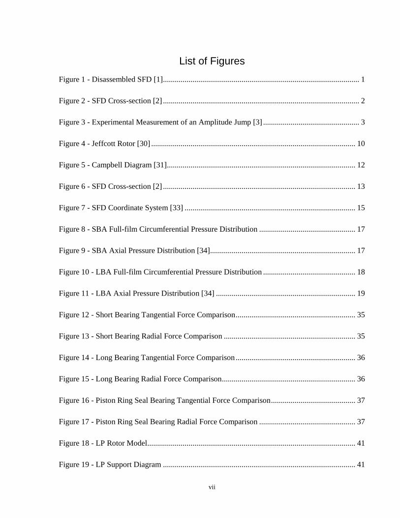
dynamic response as a sudden jump in amplitude (Fig. 3).
3
Figure 3 - Experimental Measurement of an Amplitude Jump [3]
One method of calculating the damper forces is by applying the incompressible N-S (Navier-
Stokes) equations to the lubricant film. However, due to its relative simplicity, the classical
Reynolds equation from lubrication theory is often used instead due to its relative simplicity.
The Reynolds equation is derived from the incompressible N-S equations by making several
critical assumptions about the nature of the lubricant film – the film is assumed as very thin and
inertial momentum terms are neglected. In general bearing applications, these assumptions are
valid. However, in aircraft engines, rotors move at high speeds where inertial terms are not
negligible. In a small aircraft engine, typical speeds of the LP (low pressure) and HP (high
pressure) rotor are 15 000 and 22 000 rpm, respectively. The assumption that inertial terms are
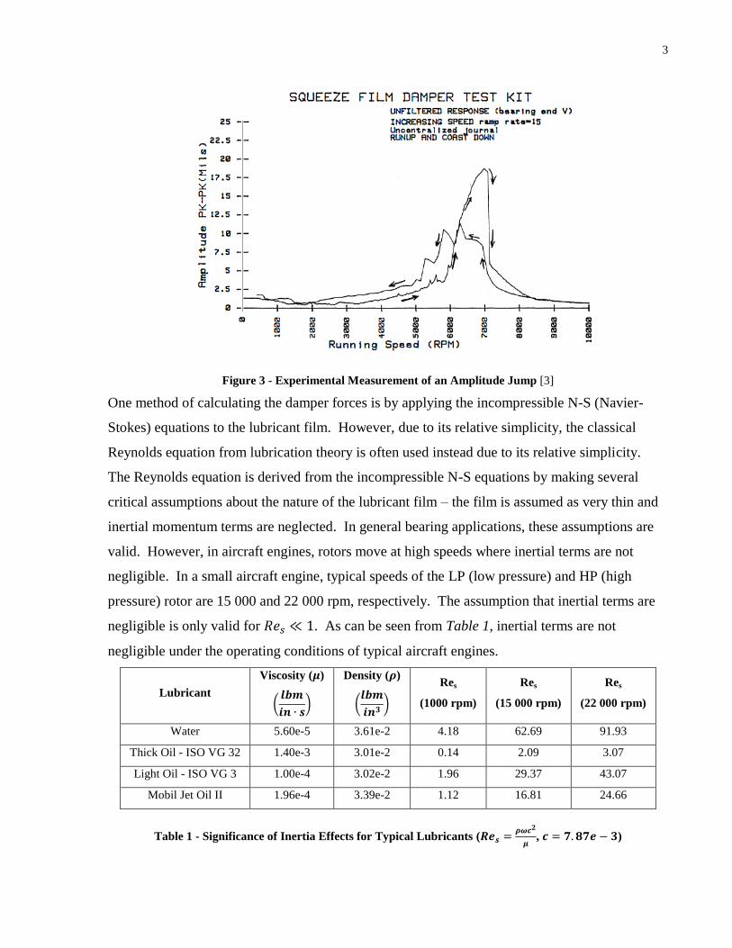
negligible is only valid for . As can be seen from Table 1, inertial terms are not
negligible under the operating conditions of typical aircraft engines.
Lubricant
Viscosity ( )
(
)
Density ( )
(
)
Res
(1000 rpm)
Res
(15 000 rpm)
Res
(22 000 rpm)
Water 5.60e-5 3.61e-2 4.18 62.69 91.93
Thick Oil - ISO VG 32 1.40e-3 3.01e-2 0.14 2.09 3.07
Light Oil - ISO VG 3 1.00e-4 3.02e-2 1.96 29.37 43.07
Mobil Jet Oil II 1.96e-4 3.39e-2 1.12 16.81 24.66
Table 1 - Significance of Inertia Effects for Typical Lubricants (
, )

4
1.1 Outline of Research
The objective of this research is to predict the transient response of an aircraft engine. The
project can be divided into two parts:
1) Determine a suitable model for the SFD
2) Model the transient response of the rotor system
As shown earlier, the Reynolds equation is not a suitable model since it neglects inertia effects
which are significant in aircraft engine operating conditions. Inclusion of the inertia effects
significantly complicates the modelling of the SFD. To fully model the incompressible N-S
equations would be ideal for obtaining the damper forces – however, the computational cost
makes this approach prohibitive. A trade-off must be made between accuracy and computational
cost. In addition, certain simplifications to the bearing model are reasonable under specific
operating conditions. The inertial effects can be categorized as temporal or convective and are
significant under different operating conditions. The thesis will investigate different SFD
models and assess their suitability under the operating conditions of an aircraft engine. Damper
forces obtained from different models are compared against experimental results.
For the second part of the thesis, the transient response of two different rotor systems is analysed
using commercial FE (finite element) software (MSC NASTRANTM
). The rotor systems have
mass and inertia distributions typical of the LP and HP rotors in a generic aircraft engine. The
response is compared between different damper models to show the influence of different inertia
effects on the dynamic response of the rotor.
1.2 Summary of Thesis Structure
Chapter 2 presents a critical review on past research related to inertia effects and the modelling
of rotordynamic systems. Chapter 3 provides the theoretical background for modelling
rotordynamic systems. Chapter 4 provides the basic theoretical background for modelling SFDs.
Chapter 5 covers different methods of modelling the inertial effects. Chapter 6 compares the
damper forces from the different bearing models. Chapter 7 compares the transient response for
the LP and HP rotor using different bearing models. Finally, conclusions and recommendations
for future research are presented in Chapter 8.

5
Chapter 2 – Literature Review
The study of rotordynamics and squeeze-film dampers is a field largely motivated by practical
applications. Rotordynamics involves studying the vibration characteristics and dynamic
response of rotating structures (e.g. compressors, turbines, turbopumps, etc.). In the 1960’s, the
need to provide damping to the rotor systems stimulated research into hydrodynamic bearings
[4]. Squeeze-film dampers were developed to avoid the stability problems associated with
hydrodynamic bearings (i.e. oil whirl). However, both types of bearings present modelling
difficulties that stimulate research to this day. A comprehensive review of the SFD as an
independent component and coupled in a rotordynamic system can be found in a two-part paper
by Della Pietra and Adiletta [5], [6]. The present review focuses on works related to the effects
of inertia on damper forces and the effect of SFDs on the dynamic response of the rotor system.
Reinhardt and Lund derived exact inertial coefficients for a finite-length journal bearing using a
first-order perturbation solution – the coefficients are accurate for [7]. They
concluded that inertial effects of the fluid film act as a virtual mass and could effectively increase
the mass of the journal by as much as 5 – 10 times. While this effect is likely negligible in large
rotors, it could be significant for small rotors. Lund et al. expanded on the perturbation solution
and derived an explicit inertial term for a circumferential groove using a bulk-flow
approximation [8]. The damper is sealed with O-rings. The same perturbation method is used to
derive a zero-order and first-order pressure. The bulk-flow model is used to describe the
conditions in the central groove. Damping and inertial coefficients are obtained from the
perturbation solution. The force coefficients are compared against experiments performed by a
test rig and there is good agreement.
Expanding on the work by Lund et al. [8], Kim and Lee included the effects of oil seals in their
analysis [9]. Kim and Lee’s analysis is specific to a short SFD with a central groove. The fluid
in the groove is considered slightly compressible. The eccentricity is assumed to be small
( ). The oil seal boundary conditions are derived by establishing a flow balance across the
seal. The axial pressure distribution is compared for three different cases: no groove effect,
groove effect and groove effect with single-stage liquid seal. The effect of the groove is
important – the inclusion of the groove significantly increases the damper forces. The theoretical

6
results are compared against experimental results from a unique test rig. The rig makes use of an
AMB (active magnetic bearing) system to apply loads to the SFD (conventional rigs apply loads
using electromagnetic shakers). This rig has several advantages over a conventional rig,
including: ease of assembly of the test SFD unit and contact-free loading. The predictions of the
model correlated well with the results obtained from measurement.
Much of the work on SFDs has come from the Tribology group at TAMU (Texas A&M
University). San Andres and Vance published several papers in 1987 that developed simple,
approximate inertial coefficients that considered the effects of either temporal or convective
inertia for finite-length bearings [10]–[12]. Force coefficients were developed based on different
journal motions, such as: small amplitude circular centered orbits, off-centered circular orbits
and large amplitude circular centered orbits. The temporal inertial coefficients considered open
bearings while the convective inertial coefficients considered both limiting geometry
configurations (short bearing and long bearing) and used an empirically determined leakage
factor to include the effects of finite leakage. San Andres and Vance have also modelled the
frequency response of rotor systems with SFD models that include the effect of inertia [13].
Recently, San Andres and Delgado have worked on improved groove models in bearings [14],
[15]. San Andres argues that modelling grooves as a constant pressure source is inaccurate –
there is fluid interaction between the groove and land that significantly affects the fluid pressure.
Rather than explicitly modelling the fluid flow, they developed an empirical model for the
groove. Force coefficients are calculated from the model and compared against experimental
results from a test rig at TAMU. They concluded that the empirical model of the groove results
in larger inertial coefficients. They also concluded that the groove cannot be modelled as an
isolated pressure source –fluid interactions between the groove and land are significant.
More detailed experiments on obtaining the bearing force coefficients are found in [16]–[18].
Different configurations of bearings were tested, including: sealing conditions, clearance size
and bearing length. The test rig consisted of two electrostatic shakers placed in orthogonal
directions to simulate journal precession. A hydraulic static loader allowed for off-centered
motion. For open dampers, piezoelectric pressure sensors were used to measure the pressure in
the film lands and groove. Similar to San Andres and Delgado, they showed that the common
assumption that the groove pressure is zero is inaccurate. The shakers applied bearing loads at a

7
constant frequency and the pressure was plotted for the duration of four periods. The frequency
of the pressure in the land was very similar to the pressure in the groove. At high frequency, the
pressure curves showed spikes which were caused by air ingestion and entrapment. The force
coefficients from the test rig were compared against the models developed in [14], [15] and
found to be in good agreement for all different bearing configurations.
Tichy has also done a significant amount of work related to the effects of fluid inertia and
viscoelasticity on SFDs [19]–[21]. In [21], Tichy derived a modified version of the Reynolds
equation using inertialess velocity profiles. This assumed that the viscous velocity profiles do
not change significantly when inertia effects are added. The modified Reynolds equation was
solved using the separation of variables technique and the corresponding eigenvalues were
obtained from a computer library routine. Tichy plotted the pressure distribution in the
circumferential direction for different values of , eccentricity and end leakage. He concluded
that the effects of inertia caused a large increase in the pressure amplitude, a change in the shape
of the pressure distribution and a phase shift of the pressure peak in the direction of the journal
precession. Also, leakage from seals significantly affected the pressure amplitude but did not
affect the pressure distribution shape or cause a phase shift. Finally, he observed that the bearing
length has a large effect on the pressure amplitude for bearings with a high leakage rate, but little
effect on bearings with tight seals.
Marmol and Vance derived pressure boundary conditions for different end seals and inlets,
including: piston rings, radial O-rings, axial O-rings and hole inlets [22]. The boundary
conditions were derived using the mass flow balance over the seal. The end seals were
dependent on an empirically determined leakage coefficient. A finite difference solution to the
Reynolds equation was also presented.
Defaye et al. performed experiments to obtain force coefficients and pressure distributions for
three different bearing configurations moving in circular-centered orbits (CCO) [23].
Experiments were performed on an SFD in a test rig with three different feeding systems:
centered feeding groove, eccentric feeding groove and equally spaced orifices. There was a non-
negligible drop in the pressure distribution in the groove fed SFDs resulting in lower tangential
damping forces. They observed that the effects of inertia increased with respect to bearing
clearance and decreased with respect to lubricant viscosity – for a centered orbit, these effects
8
manifested as an increased radial force. A characteristic trend for temporal inertia effects was
confirmed by showing that the radial force increased with respect to the whirl frequency for
constant eccentricity. On the other hand, for constant whirl frequency, the radial forces also
increased with respect to eccentricity, which is characteristic of convective effects and often
ignored. Also, Defaye et al. presented experimental results of the pressure variation in the
groove and land of the SFD for the full-film and cavitated film. They show that the pressure
variation in the groove has the same shape as that of the land. There was an offset in the peak of
the pressure curve between the groove and land which was caused by inertia effects. Finally,
they showed that lubricant in the groove can cavitate, which can result in a situation where
lubricant is not properly fed to the SFD.
Gehennin et al. presented a solution to the bulk-flow equations for SFDs using the FVM (finite
volume method) [24]. The bulk-flow equations are a simplified set of equations derived from the
Navier-Stokes equations based on the thin film assumption. The solution to the bulk-flow
equations consisted of velocity and pressure fields. The equations are solved using the SIMPLE
(semi-implicit method for pressure linked equations) algorithm – a well-established method for
solving the incompressible Navier-Stokes equations. An advantage of using the bulk-flow
equations to obtain the damper forces is that the fluid interactions at the groove and seals can be
modelled explicitly. A cavitation model is necessary because the FVM requires that flow
continuity is conserved – Gehennin et al. used a cavitation model which is based on the
Rayleigh-Plesset equation (obtained from conservation of mass and momentum on a bubble
surface). The cavitation model adjusts the density of the lubricant in the presence of bubbles so
that the mass and momentum equations remain balanced. The bulk-flow equations were
compared against a 2D model of a long bearing (constant pressure and no flow in axial direction)
in FLUENT (commercial CFD software) to test the validity of the bulk-flow equations under
high . For , the relative error of the resulting forces was ~10-15%. The forces from
the model in the tangential and radial forces were compared to the experimental results of
Defaye et al. [23] and showed close agreement.
Armentrout and Gunter present a modal method for calculating the transient response of the
rotordynamic system [25]. They demonstrated nonlinear features of the rotordynamic system
such as the jump condition. The dynamic response of an aircraft turbofan engine high pressure

9
(HP) rotor is studied for varying levels of unbalance. The SFD is modelled using the short
bearing assumption.
Bonello and Hai have developed a number of techniques for analyzing the vibrations of real
aircraft engine structures [26]–[29]. In [26], Hai and Bonello introduce the novel “impulsive
receptance method” for time domain analysis of rotor structures. In conventional FE analysis of
rotor structures, the physical structure is often transformed into a set of modal equations in order
to reduce the degrees of freedom in the system. However, the number of modes retained may
still be very large. Bonello and Hai derived a set of equations that are “essentially the inverse
Fourier transform of the frequency domain receptance/mobility equations relating the relative
displacements and velocities at the SFDs with motion-dependent forces and other excitations
acting on the linear part of the structure”. Computational efficiency is not affected by the large
number of modes but only depends on the number of nonlinear elements in the model. Bonello
and Hai also presented a frequency domain method in [27]. The method relies on obtaining the
necessary nonlinear algebraic equations by using the force-displacement relations for each
harmonic of the vibration from the frequency response functions for the linear part of the
structure (the structure without nonlinearities, e.g. SFDs).
The present literature review shows significant progress has been made in investigating the
effects of fluid inertia on damper forces. However, a definitive method for modelling the SFD
does not exist. Most damper models are not general – they are only valid under a particular set
of operating conditions (e.g. CCO, small amplitude motion, range of rotor speeds). The bulk-
flow model – which is valid for – does not have these restrictions but is
computationally expensive, making it unsuitable for use in the transient analysis of the rotor
system. In addition, the majority of research focuses on the SFD as an independent system,
instead of a component within a rotor system. The work that has been done on rotor systems rely
on simplified SFD models such which ignore important effects such as fluid inertia. The work in
this thesis will analyze the response of a rotor system using an SFD model that includes inertia
effects.

10
Chapter 3 – Rotordynamics
In this chapter, the governing equations for rotordynamic systems will be briefly covered. Also,
covered will be the concept of a critical speed, which is useful for describing the dynamic
response of the rotor system.
3.1 Governing Equations for Rotor Systems
The equation of motion for a single DOF (degree of freedom) system under forced vibration is
given by the following:
( 1 )
where M is mass, C is damping, K is stiffness, F(t) is the external applied load and q is the
generalized displacement. The notation represents the derivative of the generalized
displacement with respect to time. In a MDOF (multi-degree of freedom) system, the
coefficients become matrices and the motion is given by a system of n equations, where n is the
number of DOFs:
[ ]{ } [ ]{ } [ ]{ } { } ( 2 )
Note that {…} denotes a n x 1 vector and […] denotes an n x n matrix. An idealized rotor
system often studied is the Jeffcott rotor (Fig. 4), which consists of a flat disk supported by a
uniform, massless, flexible shaft.
Figure 4 - Jeffcott Rotor [30]

11
If the system is in free vibration and there are no bearing supports, the equation can be written
as:
[
] {
}
[ ]
{
}
[
]
{
} ( 3 )
where refers to the rotor speed of the system. Note the terms in the damping matrix which
couple the equations. These terms are a result of the gyroscopic effects of the rotor. If the
system is supported by bearings (e.g. SFDs), it is possible that the damping occurs in cross
coupled directions in addition to normal directions. The equation will then appear as:
[
] {
}
[ ]
{
}
[
]
{
} ( 4 )

12
3.2 Critical Speeds
Another effect of the gyroscopic terms is that the eigenvalues obtained from (3) and (4) are
dependent on the rotor speed ( ). This can be shown graphically using a Campbell diagram
(Fig. 5). The blue and pink curves show how the eigenvalues change with respect to – the
blue curve represents FW (forward whirl) while the pink curve represents BW (backwards whirl).
A parameter of interest is the critical speed, which can be interpreted as the rotordynamic
analogue to the natural frequency of a non-rotating system. The system is excited when the
loading frequency is equal to the whirl speed of the system. For a synchronous system, the load
frequency is equal to the rotor speed and is represented by the diagonal curve in Fig. 5. The
system is excited at frequencies where the curve crosses pink and blue curves (points A and B,
respectively) – these frequencies are defined as the critical speeds of the system.
Figure 5 - Campbell Diagram [31]

13
Chapter 4 – Squeeze Film Dampers (basic features)
In this chapter, the general features of SFDs will be discussed. First the general equations for
calculating the damper forces will be presented. Simplified analytical solutions to the equations
will be derived. Lubricant cavitation will be discussed briefly. A finite-difference solution to
the Reynolds equation will be presented. Finally, details will be given on SFD force coefficients.
Damping is introduced into an engine using squeeze film dampers. The bearing assembly is
composed of ball or roller bearings which support the rotor shaft. The bearings permit the shaft
to rotate. The bearings are housed within a journal which permits translational movement but
prohibits rotational movement via some mechanism (e.g. anti-rotation pin, spring) – this prevents
destabilizing phenomena such as oil whip [4]. The journal is encased within the bearing housing
and a thin layer of film is found between the housing and journal (thickness is in the order of a
thousandth of an inch). Damping forces are generated by squeezing an oil-film lubricant. See
Fig. 6 for a cross-section of a typical SFD. Note that the lubricant film thickness is exaggerated
for illustrative purposes.
Figure 6 - SFD Cross-section [2]
The damping forces are governed by the Navier-Stokes equations for incompressible flow, which
are as follows:
( 5 )

14
( 6 )
(
)
(
) ( 7 )
(
)
(
) ( 8 )
(
)
(
) ( 9 )
where u, v and w represent the velocity of the fluid in the x, y and z directions, respectively. p,
and is the fluid pressure, density and viscosity, respectively. t is time. The solution variables
are the fluid velocity and pressure as a function of x, y, z and t (5).
The film thickness is very small relative to the circumference of the journal. If the equations are
put in dimensionless form and an order of magnitude analysis is performed, it can be seen that
several viscous terms can be neglected [4], [32]. The remaining terms appear below.
( 10 )
(
)
( 11 )
( 12 )
(
)
( 13 )
The terms on the left-hand side of the equation are the inertial terms. The inertial terms can be
categorized as either temporal (green) or convective (blue). The film thickness of the lubricant, h
can be defined using a moving coordinate system in terms of θ, where corresponds to the
location where the film thickness h is largest (Fig. 7). e refers to the journal eccentricity (the
distance between the journal center and bearing center, OJ and OB, respectively). The

15
eccentricity is often written in dimensionless form as
, where c is the bearing clearance
(distance from outer radius of the journal to the inner radius of the housing when the bearing is
centered). Using some trigonometry, and assuming that the bearing clearance c is much smaller
the journal radius Rj, h can be defined as:
( 14 )
Figure 7 - SFD Coordinate System [33]
The flow boundary conditions across the thin film of an SFD are:
( 15 )
( 16 )
( 17 )
(16) refers to the squeezing motion of the thin film. To obtain the Reynolds equation, the inertial
terms must be neglected. In many bearing applications, the velocity of the lubricant is very small
and this is a reasonable assumption. The squeeze film Reynolds number is defined to identify
the significance of the viscous forces relative to inertial forces:
16
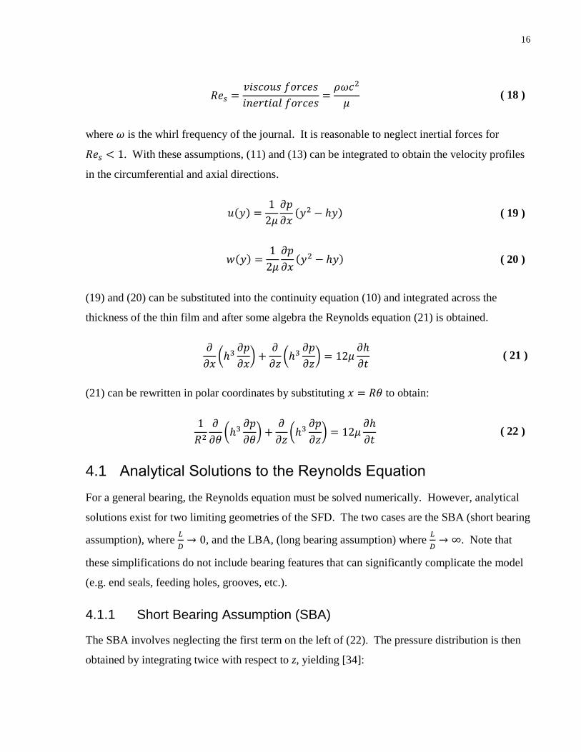
( 18 )
where is the whirl frequency of the journal. It is reasonable to neglect inertial forces for
. With these assumptions, (11) and (13) can be integrated to obtain the velocity profiles
in the circumferential and axial directions.
( 19 )
( 20 )
(19) and (20) can be substituted into the continuity equation (10) and integrated across the
thickness of the thin film and after some algebra the Reynolds equation (21) is obtained.
(
)
(
)
( 21 )
(21) can be rewritten in polar coordinates by substituting to obtain:
(
)
(
)
( 22 )
4.1 Analytical Solutions to the Reynolds Equation
For a general bearing, the Reynolds equation must be solved numerically. However, analytical
solutions exist for two limiting geometries of the SFD. The two cases are the SBA (short bearing
assumption), where
, and the LBA, (long bearing assumption) where
. Note that
these simplifications do not include bearing features that can significantly complicate the model
(e.g. end seals, feeding holes, grooves, etc.).
4.1.1 Short Bearing Assumption (SBA)
The SBA involves neglecting the first term on the left of (22). The pressure distribution is then
obtained by integrating twice with respect to z, yielding [34]:

17
[ (
)
] ( 23 )
where pambient is the ambient pressure at the bearing ends (pressure of the environment).
Physically, this assumption is valid for open bearings (ends not sealed, pressure at ends equal to
ambient pressure). The circumferential pressure distribution is similar to a reversed sine curve,
except that the peaks are sharper (Fig. 8). The SBA results in a parabolic pressure distribution in
the axial direction where the pressure is greatest at (Fig. 9). The bearing ends are located
at
.
Figure 8 - SBA Full-film Circumferential Pressure Distribution
Figure 9 - SBA Axial Pressure Distribution [34]
-6
-4
-2
0
2
4
6
0 1 2 3 4 5 6
Pre
ssu
re (
psi
)
Theta (rad)
Short Bearing Pressure Curve

18
4.1.2 Long Bearing Assumption (LBA)
The LBA involves neglecting the second term on the left of (22). The pressure distribution is
then obtained by integrating twice with respect to , yielding [35]:
[
(
( )
)] ( 24 )
Physically, this assumption is valid for bearings where the axial flow of lubricant is zero (i.e.
perfectly sealed bearings). It can be seen from (24) that pressure is not a function of z, that is,
the pressure is constant in the axial direction (Fig. 11). The peaks of the circumferential pressure
distribution are wider (Fig. 10) when compared to the short bearing (Fig. 8). Also, note that the
long bearing pressures are much greater than the short bearing – the damper forces in the long
bearing are significantly larger in the long bearing compared to the short bearing for the same
bearing geometry.
Figure 10 - LBA Full-film Circumferential Pressure Distribution
-400
-300
-200
-100
0
100
200
300
400
0 1 2 3 4 5 6
Pre
ssu
re (
psi
)
Theta (rad)
Long Bearing Pressure Curve

19
Figure 11 - LBA Axial Pressure Distribution [34]
4.2 Lubricant Cavitation
If cavitation of the lubricant is not considered, the negative pressures generated in the thin film
are comparable to the positive pressures (Fig. 8 and Fig. 10). However, in reality, the lubricant
cannot sustain large negative pressures and the lubricant cavitates as the pressure drop below the
saturated vapour pressure of the lubricant. The thin film can be separated into a “full-film”
region and the “cavitated” region – the cavitated region is not described by the Reynolds
equation [36]. It is reasonable to assume that the pressure in the cavitated region is equal to the
saturated vapour pressure. However, the exact location of the boundary between the “cavitated”
and “full-film” region is not known a priori – this is one of the principal complications of
bearing calculations. The location of the boundary condition is given by the Reynolds boundary
condition, where
|
[37]. However, in practice, the π-film model is used for simplicity
– this model assumes the boundary condition is located at . In engineering practice,
negative pressures are considered equal to zero [34]. The additional mathematics involved in
solving for the Reynolds boundary condition is significant [37]. Note – a consequence of
imposing the boundary condition is that flow continuity of lubricant is not conserved at
θcav.
4.3 Finite Difference Solution of Reynolds Equation
The solution to the Reynolds equation can be obtained numerically using the finite difference
method. The first step is to discretize the domain of the problem into a set of points called a

20
mesh. The governing differential equation is approximated by means of Taylor series expansion
so that it can be represented by values from the mesh. The Taylor series expansion is repeated
on the governing differential equation for each point on the mesh, resulting in a system of n
equations with n unknowns, where n is the number of points on the mesh. The system is then
solved using a technique for solving systems of equations (e.g. Gaussian elimination, successive
over-relaxation). Relaxation can be used to speed up convergence or assist a diverging solution.
Backwards differences are used to approximate the first order derivatives and central differences
are used to approximate the second order derivatives:
( 25 )
( 26 )
( 27 )
( 28 )
( 29 )
where i and j are the grid points in the circumferential and axial directions, respectively, a and b
are the total number of points in the circumferential and axial directions, respectively and L is the
bearing length. (25) to (28) can be substituted into (22) to obtain:
(
)
( 30 )
(30) can be rearranged to give the pressure at node i,j:
(
)( [
]
( ) [
]
( )
[
]
( ) [
]
( )
)
( 31 )

21
To solve for the pressure using successive over-relaxation, the pressure is iterated using (32)
where k is the current iteration and is the relaxation factor. (32) is successively iterated
until the change in pressure between iterations is less than 1*10-6
. The relaxation factor used is
.
( 32 )
4.4 Rotordynamic Force Coefficients
San Andres has derived several sets of force coefficients for SFDs under different operating
conditions. Force coefficients are a more direct method to obtain the damper forces – there is no
intermediary step in obtaining the pressure distribution and integrating over the damper surface
to obtain the bearing forces. However, the force coefficients are only valid under strict
assumptions (e.g. specific bearing length, seal condition, feeding condition, orbit amplitude, orbit
motion) so care must be taken to ensure the assumptions are met.
Force coefficients can be given in Cartesian ((33) and (34)) or polar coordinates ((35) and (36)).
The bars denote dimensionless terms. The first subscript denotes force direction and the second
subscript denotes velocity or acceleration direction.
( 33 )
( 34 )
[ ] [ ] ( 35 )
[ ] [ ] ( 36 )

22
Chapter 5 – Squeeze Film Dampers (inertial effects)
Inertia effects are no longer negligible in applications where Res > 1. Recall that the Reynolds
equation (22) does not include inertia effects. Inertia terms can be categorized as either temporal
or convective.
5.1 Bulk-Flow Model
In applications where both temporal and convective inertia effects are significant, the damper can
be modelled using the bulk-flow equations. These are obtained by integrating (10) to (13) across
the thin-film in the radial direction. The viscous effects ( ) are represented by wall shear
stresses that are obtained using empirically determined friction laws which are dependent on the
flow regime (e.g. Blasius, Moody).
Solution variables to the bulk-flow equations are bulk variables (37) – these represent quantities
averaged over the thin film. Solving the bulk-flow equations is more complicated and
significantly more computationally expensive when compared to the numerical solution of the
Reynolds equation. The equations can be solved using the finite-volume method and SIMPLE
algorithm [24]. However, obtaining a solution can take from minutes to hours – this method is
not practical for calculating the transient response of a rotor system where the number of time
steps in a typical calculation might be of and the damper forces must be calculated for
each time step. The bulk-flow equations are given below.
∫
∫
∫
( 37 )
( 38 )
|
( 39 )
|
( 40 )
5.2 Temporal Inertia Effects
The temporal inertia effects are represented by the green terms in (39) and (40). Different
approaches have been developed to account for their effects.

23
For small amplitude centered motion, convective inertia effects are negligible relative to
temporal inertia effects [10], [14]. Physically, this means there are different time scales for
advection and temporal terms – fluid flow can be “slow” but highly unsteady [10].
5.2.1 Temporal Force Coefficients
One method developed by San Andres involves using a set of force coefficients [10]. The
coefficients have been derived for open SFDs (the pressure at the ends are set to ambient
pressure). The method assumes the journal moves in small amplitude circular centered orbits.
First, the following dimensionless variables are introduced:
( 41 )
( 42 )
where is the squeeze-film damper clearance ratio (
). The dimensionless variables are
substituted into (10) to (13) and the convective terms (blue) are neglected to obtain the
following:
( 43 )
( 44 )
( 45 )
(44) and (45) are differentiated with respect to to eliminate the pressure term, to obtain:
( 46 )
( 47 )

24
The general solution of (46) and (47) with the boundary conditions from (15) to (17) and open
ends are of the form:
( 48 )
{
} ( 49 )
( 50 )
( 51 )
where
( 52 )
( 53 )
(
)
(
)
( 54 )
Functions F and G are related by:
{
} ( 55 )
( 56 )
For the pressure to satisfy the axial momentum equation, F and G must be related by:
( 57 )
(57) is substituted into (55) to obtain an ordinary differential equation for :

25
( 58 )
The solution for is of the form:
(
( )
) ( 59 )
Substituting (59) into (51) and only retaining the real part gives the pressure field as:
(
( )
) ( 60 )
(60) can be integrated over the bearing surface to obtain the bearing forces. The resulting force
coefficients for the full film assumption are:
( 61 )
( 62 )
(
)
(
)
(
)
(
)
( 63 )
where La is a leakage factor that accounts for the finite length of the bearing. For the π-film
assumption, the force coefficients are divided by 2.
5.2.2 Modified Reynolds Equation
Another method involves using the modified Reynolds equation [14], [15]. This equation is
derived from the bulk-flow equations. First, the convective inertia terms are ignored in (39) and
(40) since they are negligible for small amplitude centered motions [10], [14], to obtain:
|
( 64 )

26
|
( 65 )
Substituting the velocity profiles for the wall shear stress terms gives:
( 66 )
( 67 )
(66) and (67) can be rearranged in terms of bulk velocities:
( 68 )
( 69 )
Substituting (68) and (69) into (38) and neglecting second order terms yields:
(
)
(
)
( 70 )
Substituting yields:
(
)
(
)
( 71 )
The pressure and film thickness must be expressed as the superposition of a 0th
order static term
and 1st order dynamic term – these terms are then substituted into (71). For small amplitude,
circular centered orbits, closed-form solution can be obtained. This solution produces forces that
are identical to those obtained from the San Andres temporal force coefficients.
5.3 Convective Inertia Effects
The convective inertia effects are represented by the blue terms in (39) and (40). For large
amplitude journal motion, convective inertia effects are significant and should be incorporated
into the analysis. However, including the convective inertia terms is complicated – the terms are

27
nonlinear. San Andres has developed an approximate set of force coefficients to model the
effects of convective inertia using the method of averaged inertia [12]. His method is presented
here.
First, similar to the method for deriving temporal force coefficients, the solution variables to the
Navier-stokes equations are rewritten as dimensionless variables. The only difference is an
additional r term in the dimensionless pressure which depends on geometry of the bearing.
( 72 )
( 73 )
{
(
)
( 74 )
(72) and (73) are substituted into (38) to (40), the temporal terms (green) are neglected and the
equations are rewritten in a moving frame of reference to obtain the following:
( )
( )
(
) ( 75 )
[
(
)
]
( ) ( 76 )
[
(
)
]
( ) ( 77 )
(75) to (77) are integrated over the thin-film thickness in the direction to obtain a system of
integro-differential equations:
( 78 )
[
]
( 79 )
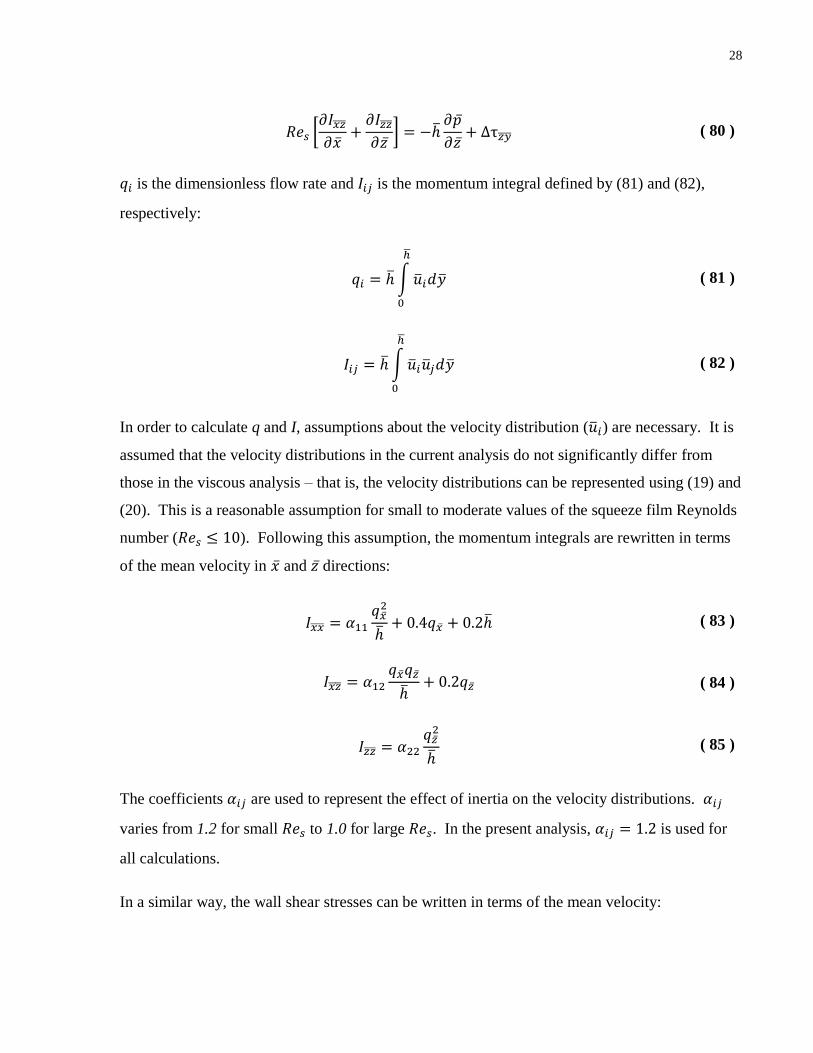
28
[
]
( 80 )
is the dimensionless flow rate and is the momentum integral defined by (81) and (82),
respectively:
∫
( 81 )
∫
( 82 )
In order to calculate q and I, assumptions about the velocity distribution ( ) are necessary. It is
assumed that the velocity distributions in the current analysis do not significantly differ from
those in the viscous analysis – that is, the velocity distributions can be represented using (19) and
(20). This is a reasonable assumption for small to moderate values of the squeeze film Reynolds
number ( ). Following this assumption, the momentum integrals are rewritten in terms
of the mean velocity in and directions:
( 83 )
( 84 )
( 85 )
The coefficients are used to represent the effect of inertia on the velocity distributions.
varies from 1.2 for small to 1.0 for large . In the present analysis, is used for
all calculations.
In a similar way, the wall shear stresses can be written in terms of the mean velocity:
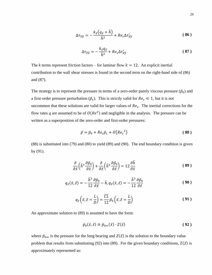
29
( )
( 86 )
( 87 )
The k terms represent friction factors – for laminar flow . An explicit inertial
contribution to the wall shear stresses is found in the second term on the right-hand side of (86)
and (87).
The strategy is to represent the pressure in terms of a zero-order purely viscous pressure ( ) and
a first-order pressure perturbation ( ). This is strictly valid for , but it is not
uncommon that these solutions are valid for larger values of . The inertial corrections for the
flow rates q are assumed to be of and negligible in the analysis. The pressure can be
written as a superposition of the zero-order and first-order pressures:
( ) ( 88 )
(88) is substituted into (79) and (80) to yield (89) and (90). The end boundary condition is given
by (91).
(
)
(
)
( 89 )
( 90 )
(
)
(
) ( 91 )
An approximate solution to (89) is assumed to have the form:
( 92 )
where is the pressure for the long bearing and is the solution to the boundary value
problem that results from substituting (92) into (89). For the given boundary conditions, is
approximately represented as:

30
( 93 )
( )
( )
( 94 )
The solution to the first-order pressure field can be written approximately as:
[
]
[
( )]
( 95 )
After determining and from (92) and (95), the pressure field can be integrated over the
bearing surface to obtain the bearing forces to obtain the force coefficients. The force
coefficients depend on a number of different parameters and are summarized in the Appendices
for brevity.

31
Chapter 6 – Comparison of Inertial Damper Models
From Chapter 3, we have covered several different methods for modelling the damper inertial
effects. In the present chapter, the forces from the temporal and convective inertial models will
be compared against the inertialess Reynolds equation to highlight the differences. The forces
will be plotted for the two limiting geometry cases (short bearing and long bearing). Finally,
forces will be plotted for a bearing with a piston ring seal and compared against experimental
results presented by Defaye et al. [23].
6.1 Bearing Geometry
The bearing geometry is taken from Defaye et al. [23] and summarized in Table 2. The bearing
is fed from a centered groove (in the middle of the land). The piston ring seal is modelled using
the boundary conditions found from Marmol and Vance [22].
Note that the damper models from the previous section have not modelled the effect of the
groove. In the past, researchers have considered the groove as a source of constant pressure [22],
however, experimental results from Defaye et al. show that this is inaccurate – there is fluid
interaction between the land and groove. Due to the nature of its complexity, the effect of the
groove is not considered in this thesis – it is recommended that this be a topic of future study.
SFD Parameters
Bearing
Diameter 6 in
Length 1.38 in
Clearance 7.87*10-3
in
Lubricant (Mobil Jet Oil II)
Viscosity 1.96*10-4
lbm/(in*s)
Density 3.389*10-2
lbm/in3
Table 2 - SFD Parameters

32
6.2 Operating Conditions
The journal is assumed to move in CCO – the journal eccentricity is assumed as constant
( ). The whirl frequency is assumed as a constant value of – for
the given bearing geometry, this corresponds to a squeeze Reynolds number of Res=3.90. The
tangential and radial forces from the damper are plotted for five different dimensionless
eccentricities .
6.3 Bearing Models
The following bearing models will be considered in this chapter: Reynolds equation, San Andres
temporal force coefficients [11] and San Andres convective force coefficients [12]. The San
Andres temporal force coefficients will only be considered in the short bearing case since the
model has not been developed for long or sealed bearings. The bulk-flow model is not
considered since its computational cost makes it impractical for use in dynamic model of the
rotor system.
6.4 Comparison of Damper Forces
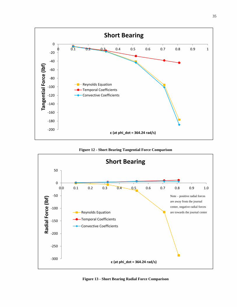
Fig. 12 and 13 show the tangential and radial forces for the short bearing, respectively, while
Fig. 14 and 15 show the tangential and radial forces for the long bearing, respectively. These
two limiting cases establish the lower and upper bounds for the damper forces, respectively – the
forces obtained from the piston ring sealed bearing (finite leakage) will be in-between the two
limiting cases.
In Fig. 12, it can be seen that for , the forces from the different models are relatively
close in magnitude, with the temporal coefficient model being the exception. This may be
caused by the fact that the temporal model is only valid for small amplitude orbits – may
be the limit at which the temporal coefficient model is valid.
In Fig. 13, the inertial models have greater radial forces when compared against the inertialess
Reynolds equation – this is consistent to the “added mass” effect reported in literature [5], [7],
[23]. The forces obtained from the temporal and convective models are significantly different –
the direction of forces from the Reynolds equation are faced towards the journal center while the
direction of forces from the temporal and convective models are faced away from the journal

33
center. Also, in the temporal model, the radial force appears to linearly increase with respect to
eccentricity while in the convective model, the increase in radial force begins to taper at
and the radial force decreases when .
For the long bearing, the bearing models are in close agreement for the tangential forces (Fig.
14). Note that for the short bearing, the forces show a parabolic-like relationship with respect to
eccentricity while for the long bearing, the relationship is almost linear. The radial forces in Fig.
15 show similar trends to Fig. 13 – the only difference is the radial force begins to decrease at a
lower eccentricity ( ).
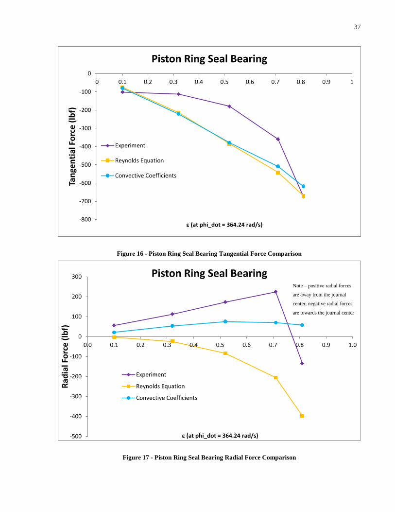
For the piston sealed bearing tangential forces in Fig. 16, it appears that the theoretical models
exhibit the linear behaviour similar to the long bearing case. However, the experimental forces
have a parabolic shape more similar to the short bearing case. It seems that the damper models
significantly over predict the magnitude of the tangential forces from .
For the radial forces in Fig. 17, it can be seen that inertia effects significantly increase the radial
forces in the direction away from the journal center. This effect is significant as it changes the
direction of the force in the convective and experimental models. Note that the convective force
coefficients best resemble the trends of the experimental results – the radial forces are faced
away from the journal center and begin to decrease after a certain eccentricity. However, there
are a number of features that are not captured by the convective force coefficient model. The
experimental forces are significantly larger than those predicted by the theoretical models. In
addition, the decrease in radial force is very sudden and the change in force is very large
compared to the convective model, where the decrease in force is gradual and comparatively
small.
The discrepancy between the experimental results and theoretical models are likely caused by
simplifying assumptions used to develop the models. As stated early in this chapter, the effects
of the feeding grooves were not considered in theoretical models. Another simplification is that
cavitation is modeled using the π-film model. Adopting a more sophisticated damper model can
improve the accuracy of the damper forces at the cost of computation time, as Gehannin et al.
have done [24]. However, if the objective is to obtain the dynamic response of the rotor system,
some compromise must be made between the accuracy of the bearing model and its

34
computational cost.
35
Figure 12 - Short Bearing Tangential Force Comparison
Figure 13 - Short Bearing Radial Force Comparison
-200
-180
-160
-140
-120
-100
-80
-60
-40
-20
0
0 0.1 0.2 0.3 0.4 0.5 0.6 0.7 0.8 0.9 1
Tan
gen
tial
Fo
rce
(lb
f)
ε (at phi_dot = 364.24 rad/s)
Short Bearing
Reynolds Equation
Temporal Coefficients
Convective Coefficients
-300
-250
-200
-150
-100
-50
0
50
0.0 0.1 0.2 0.3 0.4 0.5 0.6 0.7 0.8 0.9 1.0
Rad
ial F
orc
e (
lbf)
ε (at phi_dot = 364.24 rad/s)
Short Bearing
Reynolds Equation
Temporal Coefficients
Convective Coefficients
Note – positive radial forces
are away from the journal
center, negative radial forces
are towards the journal center

36
Figure 14 - Long Bearing Tangential Force Comparison
Figure 15 - Long Bearing Radial Force Comparison
-3500
-3000
-2500
-2000
-1500
-1000
-500
0
0 0.1 0.2 0.3 0.4 0.5 0.6 0.7 0.8 0.9 1
Tan
gen
tial
Fo
rce
(lb
f)
ε (at phi_dot = 364.24 rad/s)
Long Bearing
Reynolds Equation
Convective Coefficients
-3500
-3000
-2500
-2000
-1500
-1000
-500
0
500
0.0 0.1 0.2 0.3 0.4 0.5 0.6 0.7 0.8 0.9 1.0
Rad
ial F
orc
e (
lbf)
ε (at phi_dot = 364.24 rad/s)
Long Bearing
Reynolds Equation
Convective Coefficients
Note – positive radial forces
are away from the journal
center, negative radial forces
are towards the journal center
37
Figure 16 - Piston Ring Seal Bearing Tangential Force Comparison
Figure 17 - Piston Ring Seal Bearing Radial Force Comparison
-800
-700
-600
-500
-400
-300
-200
-100
0
0 0.1 0.2 0.3 0.4 0.5 0.6 0.7 0.8 0.9 1
Tan
gen
tial
Fo
rce
(lb
f)
ε (at phi_dot = 364.24 rad/s)
Piston Ring Seal Bearing
Experiment
Reynolds Equation
Convective Coefficients
-500
-400
-300
-200
-100
0
100
200
300
0.0 0.1 0.2 0.3 0.4 0.5 0.6 0.7 0.8 0.9 1.0
Rad
ial F
orc
e (
lbf)
ε (at phi_dot = 364.24 rad/s)
Piston Ring Seal Bearing
Experiment
Reynolds Equation
Convective Coefficients
Note – positive radial forces
are away from the journal
center, negative radial forces
are towards the journal center
38
Chapter 7 – Transient Response of a Rotor System
The effect of the SFD is most significant when the rotor traverses a critical speed. In industry, it
is common to run a ramp-up test, where a rotor is run from rest to its operating speed. The test is
intended to capture the steady-state response of the system throughout its entire operating range.
During the run the rotor will traverse through several critical speeds. An imbalance load is
applied that is typical due to limitations in manufacturing tolerances.
In the present chapter, the transient response will be obtained for two different rotor systems.
The models are representative of the LP and HP rotors in a generic aircraft engine in terms of
mass and inertia distributions. The models also cover different speed ranges. An SFD is present
in both rotor systems and the damper forces are obtained using the different models from
Chapter 6 (Reynolds equation, temporal force coefficients, convective force coefficients).
Conclusions are drawn based on the results of the analysis.
7.1 Solution Methodology
FE models of generic rotor systems are developed. Beam elements are used instead of solid
elements to reduce the model size. This is a reasonable assumption since most components on
the rotor systems can be considered to have axisymmetric geometry. The objective of the
analysis is to draw conclusions based on the differences between damper models so
exceptionally detailed models of the rotor systems is not critical. Disks in the rotor systems are
modelled as lumped masses.
The SFD forces are included in the transient analysis using a user-defined element. The user-
defined element is a section of C++ code that calculates the damper forces based on the
displacements, velocities and acceleration of the journal – these inputs are generated by the FE
code. NASTRAN includes the damper forces as external forces – they are included as on
the right-hand side of (2).
First, the critical speeds are calculated using NASTRAN to show where the peaks of the rotor
systems should be expected. Then the transient response is calculated and the displacement is
plotted with respect to time for different damper models.

39
7.2 Model Assumptions
7.2.1 Rotor Simulation
The ramp-up test is not intended to simulate the actual acceleration rate in the engine – it is
intended to simulate a steady-state sweep over the operating range of the engine. The analysis
cannot be done with a frequency response calculation because the frequency response calculation
assumes the external applied forces are harmonic and the SFD forces are nonlinear. To simulate
a steady-state sweep, the acceleration rate of the rotor is reduced and the response is calculated –
these steps are repeated until there is no change in the solution content (displacements, velocities,
accelerations, forces). It was found that reducing the acceleration rate below 157 rad/s2 had no
impact on the solution content.
7.2.2 Temporal Force Coefficients
The temporal force coefficients [10] assumes that the amplitude motions of the journal are small.
This may not be true at the critical speeds of the rotor system.
7.2.3 Convective Force Coefficients
The convective force coefficients [12] assume that the journal moves in CCO – this means that
the whirl acceleration rate and change in eccentricity is zero ( ).
This is a reasonable assumption since and are relatively small and the rotor simulation is
intended to be operating at “steady-state”.
7.3 Rotor and Bearing Models
The shaft and disk of the rotor models are assumed to be made of solid steel (Table 3).
Material Properties (steel)
Young’s Modulus (E) 30 ksi
Density ( ) 0.283 lbm/in3
Poisson’s Ratio ( ) 0.29
Table 3 - Rotor Material Properties

40
7.3.1 Low Pressure (LP) Rotor
The LP rotor is composed of a shaft with two disk and two supports (Fig. 18). One support is
located between the two disks and the other is at the end. The end support consists of a stiff
spring (2*105 lbf/in) and a linear damper (20 lbf/(in/s)) in parallel (Fig. 19). The SFD is located
at the first support. The supports are attached to the ground which is assumed to be stationary.
For the imbalance response analysis, an imbalance of 0.5 oz-in is applied to both disks. The
analysis is run for 20 s during which the system rotates from rest to 1570 rad/s (15000 rpm) at a
constant acceleration of 78.5 rad/s2. During the run, the system passes through three critical
speeds (Table 4). The response of the system with a linear damper of (20 lbf/(in/s)) instead of an
SFD at Support #1 is shown in Fig. 20.
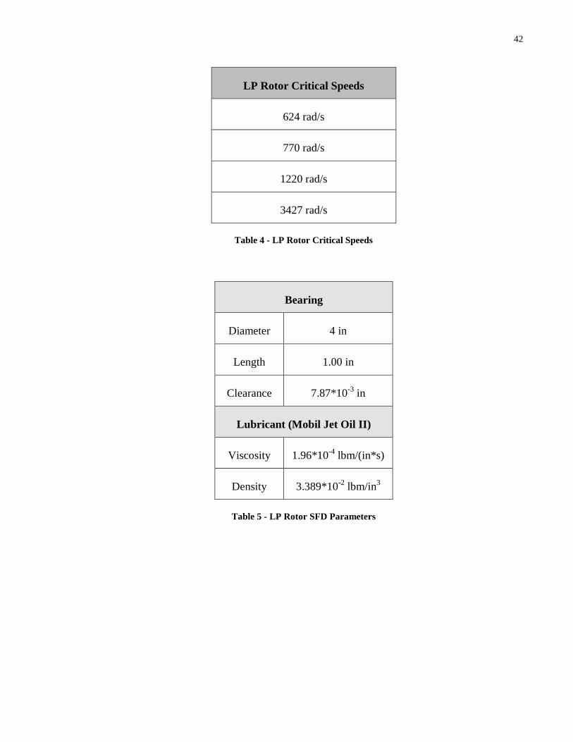
Initially, the bearing geometry from the previous chapter (Table 2) was used. However, the
solution was not stable. A smaller bearing was then used instead – its properties are summarized
in Table 5. The transient analysis was performed for the open bearing. A solution could not be
obtained for the long bearing and piston ring bearing due to issues with convergence – further
investigation is necessary to determine the cause.
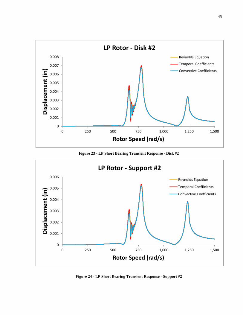
The peaks in Fig. 21 - Fig. 24 correspond to the critical speed values in Table 4. For open
bearings, there are large oscillations in the displacement after the first peak – this may be
because the damper forces are not large enough to adequately suppress the effects of the critical
speed. The time steps in the transient run were decreased from 2.5*10-5
to 4.0*10-6
with no
change in solution.
There is no frequency shift in the peaks using the different models and the curves are virtually
identical – this suggests that inertia effects are negligible for this range of operating speeds. The
squeeze Reynolds number is equal to Res=16.82 for the given bearing at 1570 rad/s. The slight
differences in amplitudes of the peaks are likely because the coefficient models are only
approximate.

41
Figure 18 - LP Rotor Model
Figure 19 - LP Support Diagram
42
LP Rotor Critical Speeds
624 rad/s
770 rad/s
1220 rad/s
3427 rad/s
Table 4 - LP Rotor Critical Speeds
Bearing
Diameter 4 in
Length 1.00 in
Clearance 7.87*10-3
in
Lubricant (Mobil Jet Oil II)
Viscosity 1.96*10-4
lbm/(in*s)
Density 3.389*10-2
lbm/in3
Table 5 - LP Rotor SFD Parameters

43
Figure 20 - LP Linear Damper Transient Response - Support #1
0
0.0005
0.001
0.0015
0.002
0.0025
0.003
0.0035
0 250 500 750 1,000 1,250 1,500
Dis
pla
cem
en
t (i
n)
Rotor Speed (rad/s)
LP Rotor - Support #1
Linear Damper

44
Figure 21 - LP Short Bearing Transient Response - Disk #1
Figure 22 - LP Short Bearing Transient Response - Support #1
0.000
0.002
0.004
0.006
0.008
0.010
0.012
0 250 500 750 1,000 1,250 1,500
Dis
pla
cem
en
t (i
n)
Rotor Speed (rad/s)
LP Rotor - Disk #1
Reynolds Equation
Temporal Coefficients
Convective Coefficients
0
0.001
0.002
0.003
0.004
0.005
0.006
0 250 500 750 1,000 1,250 1,500
Dis
pla
cem
en
t (i
n)
Rotor Speed (rad/s)
LP Rotor - Support #1
Reynolds Equation
Temporal Coefficients
Convective Coefficients
45
Figure 23 - LP Short Bearing Transient Response - Disk #2
Figure 24 - LP Short Bearing Transient Response - Support #2
0
0.001
0.002
0.003
0.004
0.005
0.006
0.007
0.008
0 250 500 750 1,000 1,250 1,500
Dis
pla
cem
en
t (i
n)
Rotor Speed (rad/s)
LP Rotor - Disk #2 Reynolds Equation
Temporal Coefficients
Convective Coefficients
0
0.001
0.002
0.003
0.004
0.005
0.006
0 250 500 750 1,000 1,250 1,500
Dis
pla
cem
en
t (i
n)
Rotor Speed (rad/s)
LP Rotor - Support #2
Reynolds Equation
Temporal Coefficients
Convective Coefficients

46
7.3.2 High Pressure (HP) Rotor
The HP rotor is composed of a single disk. Supports are located at both ends – the supports
consist of a stiff spring (2*105 lbf/in) and linear damper in parallel. At the first critical speed, the
ends act as nodes (minimal change in amplitude at resonant frequency). Consequently, placing
the SFD at the supports would be ineffective in changing the dynamic response of the system.
For this reason, the SFD is placed at the disk instead.
For the imbalance response analysis, an imbalance of 0.5 oz-in is applied to the disk. The
analysis is run for 20 s during which the system rotates from rest to 3140 rad/s (30000 rpm) at a
constant acceleration of 157 rad/s2 during the run, the system passes through one critical speed
(Table 6). The response of the system with no SFD is shown in Fig. 27.
The bearing geometry from the previous chapter is used – for convenience, the geometry is
restated in Table 7. The transient analysis was performed for the open bearing and piston ring
bearing. Similar to the LP rotor, a solution could not be obtained for the long bearing.
From Fig. 27, it can be seen that for the undamped case, the frequency at which the peak occurs
corresponds to the critical speed value in Table 6. In Fig. 28 and Fig. 29, the curves have the
same shape but smaller amplitudes – the additional inertial damping reduces the overall
displacement of the disk and supports. Furthermore, the effect of inertia can be seen when
comparing the curve from the Reynolds equation to the other curves. First, the frequency at
which the peak occurs is shifted to the left. The temporal inertia model has larger amplitudes at
the peak compared to the inertialess Reynolds equation. On the other hand, the convective
model has a smaller amplitude peak. The overall displacement once the system reaches its
operating speed is lower for the inertia models by ~ 15-30%. It is worth noting that the curves
are virtually identical up to ~ 1100 rad/s – in this operating range the effects of inertia are
negligible.
For the sealed bearing in Fig. 30 and 31, the damper forces are large enough to suppress the
effects of the critical speed – the displacements are an order of magnitude smaller compared to
the open bearing. The trends are similar in the sealed bearing – the inertial models have a
smaller overall displacement. The curves are somewhat similar and the difference in
displacements is somewhat small for speeds below 1000 rad/s. The curves are virtually identical

47
from 0-200 rpm. The smaller range of speeds for which the curves are similar may be caused by
the fact that the radial forces are much larger in the sealed bearing. It seems somewhat
reasonable to neglect inertia effects for speeds below 1000 rad/s. For the given damper, the
squeeze Reynolds number is Res=33.63 at 3140 rad/s.
Figure 25 - HP Rotor Model
Figure 26 - HP Support Diagram
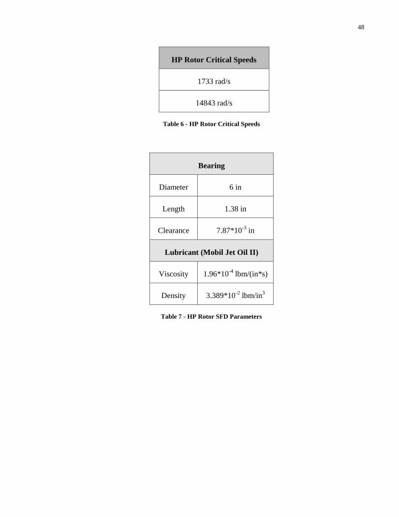
48
HP Rotor Critical Speeds
1733 rad/s
14843 rad/s
Table 6 - HP Rotor Critical Speeds
Bearing
Diameter 6 in
Length 1.38 in
Clearance 7.87*10-3
in
Lubricant (Mobil Jet Oil II)
Viscosity 1.96*10-4
lbm/(in*s)
Density 3.389*10-2
lbm/in3
Table 7 - HP Rotor SFD Parameters

49
Figure 27 - HP No Damper Transient Response - Disk
0.0000
0.0020
0.0040
0.0060
0.0080
0.0100
0.0120
0 500 1,000 1,500 2,000 2,500 3,000
Dis
pla
cem
en
t (i
n)
Rotor Speed (rad/s)
HP Rotor - Disk
No Damper

50
Figure 28 - HP Short Bearing Transient Response - Support
Figure 29 - HP Short Bearing Transient Response – Disk
0.0000
0.0005
0.0010
0.0015
0.0020
0.0025
0 500 1,000 1,500 2,000 2,500 3,000
Dis
pla
cem
en
t (i
n)
Rotor Speed (rad/s)
HP Rotor - Support
Reynolds Equation
Temporal Coefficients
Convective Coefficients
0.0000
0.0005
0.0010
0.0015
0.0020
0.0025
0.0030
0.0035
0.0040
0.0045
0 500 1,000 1,500 2,000 2,500 3,000
Dis
pla
cem
en
t (i
n)
Rotor Speed (rad/s)
HP Rotor - Disk
Reynolds Equation
Temporal Coefficients
Convective Coefficients

51
Figure 30 - HP Piston Ring Bearing Transient Response – Support
Figure 31 - HP Piston Ring Bearing Transient Response - Disk
0.0000
0.0001
0.0002
0.0003
0.0004
0.0005
0.0006
0 500 1,000 1,500 2,000 2,500 3,000
Dis
pla
cem
en
t (i
n)
Rotor Speed (rad/s)
HP Rotor - Support
Reynolds Equation
Convective Coefficients
0.0000
0.0001
0.0002
0.0003
0.0004
0.0005
0.0006
0.0007
0.0008
0.0009
0 500 1,000 1,500 2,000 2,500 3,000
Dis
pla
cem
en
t (i
n)
Rotor Speed (rad/s)
HP Rotor - Disk
Reynolds Equation
Convective Coefficients

52
Chapter 8 – Conclusions
Different inertia models were compared to observe the effects of inertia on damper forces in
Chapter 6. The main observed effect was that the radial forces were greater in the inertia
models. The forces were calculated at a squeeze Reynolds number of Res=3.90. The increase in
radial force was very significant in the inertia models. One key difference between these two
models is that for the temporal model, the radial forces increase linearly with respect to
eccentricity. On the other hand, for the convective model, the radial forces decrease after a
critical eccentricity value. This behavior is also seen in published experimental results by
Defaye et al. [23] and the cause is believed to be from lubricant cavitation. The decrease in
radial force is very sudden in the results from experiment. More study in the cavitation
phenomena would be beneficial.
The transient response was analysed for a generic LP and HP rotor operating under different
speed ranges. The displacement curves were virtually identical for the different damper models
in the LP rotor. The squeeze Reynolds number at the operating speed (15000 rpm) of the LP
rotor is Res=16.82. This indicates that even though inertial forces are present, they are not large
enough to have any impact on engine response.
For the HP rotor, the displacement curves were shifted to the left in the open bearing inertia
models – inertia effects reduce the frequency at which the peaks occur. In addition, at the
operating speed (30000 rpm), the displacements of the rotor system were smaller with the inertial
models. At the peak, the temporal model shows a slight increase in amplitude while the
convective model shows a decrease in amplitude. Similar trends were seen in the sealed bearing
displacement curves. The squeeze Reynolds number at the operating speed (30000 rpm) of the
HP rotor is Res=33.63. Overall, the effects of inertia on engine response are:
(1) Reduction in the frequency at which the peak occurs;
(2) Reduction of rotor displacement at its operating speed.
53
8.1 Recommendations for Future Work
Extensions to current research can be made in a number of different areas.
(i) Boundary Conditions: Features such as the groove and end seals are not well modelled.
Defaye et al. [23] have shown that there is strong fluid interaction between the damper
groove and land – the common assumption that models the groove as an independent
source of constant pressure is incorrect. In addition, the inertial coefficient damper
models in this thesis have not included the effect of the groove.
(ii) Cavitation: In the experimental results by Defaye et al. [23], a sudden drop in the radial
damper force is attributed to the onset of cavitation – this effect is not predicted by the π-
film model. Accurate prediction of this effect would help prevent undesirable instabilities
from occurring in the rotor structure.
(iii) Experimental Validation: It would be advisable to validate the current conclusions with
experimental results from a rotor test rig. There may be differences between the
theoretical and physical models that have not been anticipated.

54
References
[1] L. Industries, “Squeeze Film Damper Bearings,” Lufkin, 2013. [Online]. Available:
http://www.lufkin.com/index.php/products-a-services/power-transmission/bearings-and-
seals/squeeze-film-damper-bearings. [Accessed: 17-Jul-2014].
[2] L. San Andrés, “Squeeze Film Dampers: Operation, Models and Technical Issues,”
Modern Lubrication Theory, 2010. [Online]. Available:
http://repository.tamu.edu/handle/1969.1/93197. [Accessed: 13-Jul-2014].
[3] F. Zeidan, “Design and application of squeeze film dampers in rotating machinery,” Proc.
25th Turbomach. Symp., 1996.
[4] D. Childs, “Turbomachinery Rotordynamics,(1993),” John Wiley Sons, New York.
[5] L. Della Pietra and G. Adiletta, “The squeeze film damper over four decades of
investigations. Part I: Characteristics and operating features,” Shock Vib. Dig., 2002.
[6] G. Adiletta and L. Della Pietra, “The squeeze film damper over four decades of
investigations. Part II: Rotordynamic analyses with rigid and flexible rotors,” Shock Vib.
Dig., 2002.
[7] E. Reinhardt and J. W. Lund, “The influence of fluid inertia on the dynamic properties of
journal bearings,” J. Lubr. Technol., vol. 97, p. 159, 1975.
[8] J. W. Lund, C. M. Myllerup, and H. Hartmann, “Inertia Effects in Squeeze-Film Damper
Bearings Generated by Circumferential Oil Supply Groove,” J. Vib. Acoust., vol. 125, no.
4, p. 495, Oct. 2003.
[9] K.-J. Kim and C.-W. Lee, “Dynamic Characteristics of Sealed Squeeze Film Damper
With a Central Feeding Groove,” J. Tribol., vol. 127, no. 1, p. 103, Jan. 2005.
[10] L. S. Andres and J. Vance, “Effect of fluid inertia on squeeze-film damper forces for
small-amplitude circular-centered motions,” ASLE Trans., 1987.

55
[11] L. S. Andres and J. Vance, “Force coefficients for open-ended squeeze-film dampers
executing small-amplitude motions about an off-center equilibrium position,” ASLE
Trans., 1987.
[12] L. S. Andres and J. Vance, “Effects of fluid inertia on finite-length squeeze-film
dampers,” ASLE Trans., 1987.
[13] L. A. San Andres and J. M. Vance, “Effect of Fluid Inertia on the Performance of Squeeze
Film Damper Supported Rotors,” J. Eng. Gas Turbines Power, vol. 110, no. 1, p. 51, Jan.
1988.
[14] A. Delgado and L. S. Andrés, “A model for improved prediction of force coefficients in
grooved squeeze film dampers and oil seal rings,” J. Tribol., 2010.
[15] L. S. Andrés and A. Delgado, “A Novel Bul -Flow Model for Improved Predictions of
Force Coefficients in Grooved Oil Seals Operating Eccentrically,” J. Eng. Gas Turbines
Power, vol. 134, no. 5, p. 052509, May 2012.
[16] L. San Andrés and S. Seshagiri, “Damping and Inertia Coefficients for Two End Sealed
Squeeze Film Dampers With a Central Groove: Measurements and Predictions,” J. Eng.
Gas Turbines Power, vol. 135, no. 11, p. 112503, Sep. 2013.
[17] L. San Andrés, “Damping and Inertia Coefficients for Two Open Ends Squeeze Film
Dampers With a Central Groove: Measurements and Predictions,” J. Eng. Gas Turbines
Power, vol. 134, no. 10, p. 102506, Oct. 2012.
[18] L. S. Andres, “Force coefficients for a large clearance open ends squeeze film damper
with a central feed groove: Experiments and predictions,” Tribol. Int., vol. 71, pp. 17–25,
Mar. 2014.
[19] J. A. Tichy, “Effects of Fluid Inertia and Viscoelasticity on Squeeze-Film Bearing
Forces,” A S L E Trans., vol. 25, no. 1, pp. 125–132, Jan. 1982.
[20] J. A. Tichy and P. Bourgin, “The Effect of Inertia in Lubrication Flow Including Entrance
and Initial Conditions,” J. Appl. Mech., vol. 52, no. 4, p. 759, Dec. 1985.

56
[21] J. A. Tichy, “A Study of the Effect of Fluid Inertia and End Lea age in the Finite Squeeze
Film Damper,” J. Tribol., vol. 109, no. 1, p. 54, Jan. 1987.
[22] R. A. Marmol and J. M. Vance, “Squeeze Film Damper Characteristics for Gas Turbine
Engines,” J. Mech. Des., vol. 100, no. 1, p. 139, Jan. 1978.
[23] C. Defaye, M. Arghir, O. Bonneau, P. Carpentier, C. Debailleux, and F. Imbourg,
“Experimental Study of the Radial and Tangential Forces in a Whirling Squeeze Film
Damper,” Tribol. Trans., vol. 49, no. 2, pp. 271–278, Jul. 2006.
[24] J. Gehannin, M. Arghir, and O. Bonneau, “Complete Squeeze-Film Damper Analysis
Based on the ‘Bul Flow’ Equations,” Tribol. Trans., 2009.
[25] R. Armentrout and E. Gunter, “TRANSIENT MODAL ANALYSIS OF NONLINEAR
ROTOR-BEARING SYSTEMS,” sem-proceedings.com.
[26] P. M. Hai and P. Bonello, “An impulsive receptance technique for the time domain
computation of the vibration of a whole aero-engine model with nonlinear bearings,” J.
Sound Vib., vol. 318, no. 3, pp. 592–605, Dec. 2008.
[27] P. Bonello and P. Minh Hai, “A receptance harmonic balance technique for the
computation of the vibration of a whole aero-engine model with nonlinear bearings,” J.
Sound Vib., vol. 324, no. 1–2, pp. 221–242, Jul. 2009.
[28] P. Bonello and P. M. Hai, “Computational Studies of the Unbalance Response of a Whole
Aero-Engine Model With Squeeze-Film Bearings,” J. Eng. Gas Turbines Power, vol. 132,
no. 3, p. 032504, Mar. 2010.
[29] P. Bonello, P. Hai, and K. Groves, “Calculation of the Unbalance Response of Whole
Aero-Engine Models,” w3.uniroma1.it.
[30] J. RÉDL and V. KROCKO, “Mathematical model of Jeffcott rotor supported on slide
bearings assembly,” Kraj. J., PISZCZALKA J., KOL, 2009.
[31] Halpaugh, “Campbelldiagram.” [Online]. Available:
http://en.wikipedia.org/wiki/File:Campbelldiagram.png. [Accessed: 13-Jul-2014].

57
[32] O. Pinkus and B. Sternlicht, Theory of hydrodynamic lubrication. McGraw-Hill, 1961.
[33] L. San Andrés, “Kinematics of Journal Bearings,” Modern Lubrication Theory, 2012.
[Online]. Available: http://repository.tamu.edu/handle/1969.1/93197. [Accessed: 13-Jul-
2014].
[34] L. San Andrés, “Static Load Performance of Plain Journal Bearings,” Modern Lubrication
Theory, 2010. [Online]. Available: http://repository.tamu.edu/handle/1969.1/93197.
[Accessed: 13-Jul-2014].
[35] J. Vance, Rotordynamics of turbomachinery. 1988.
[36] L. Floberg, On hydrodynamic lubrication with special reference to sub-cavity pressures
and number of streamers in cavitation regions. Stockholm: Royal Swedish Academy of
Engineering Sciences, 1965.
[37] A. Cameron, The principles of lubrication, vol. 132. Longmans London, 1966.

58
Appendices
A - 1
A - 2
A - 3
A - 4
A - 5
A - 6
A - 7
A - 8
A - 9
A - 10
(
)
A - 11
A - 12
A - 13

59
∫
A - 14
∫
[
] A - 15
∫ (
)
[
] A - 16
A - 17
(
)
A - 18
(
)
( ) (
)
A - 19
A - 20
A - 21
A - 22