Fluid Flow MeasurementFluid Flow MeasurementObjective of measurement is either:

Velocity, orFlow rate (mass or volumetric).

Methods used may be categorized as:1. Primary or quantity methods:

a. Weight or volume tanks, burettes, etc.b. Positive displacement meters

i. “Water” meterii. Wet test meter (measures gas flow)

Categories of Measurement2. Secondary or rate devices:

a. Obstruction metersi. Venturiii. Flow Nozzlesiii. Orifice

b. Variable Areai. Vertical rotameterii. Spring-loaded rotameter

Categories (Cont’d)

c. Velocity probesi. Pitot tubeii. Anemometer (propeller)iii. Hot-wire anemometer

d. Special methodsi. Turbine metersii. Paddlewheel metersiii. Thermal mass flow metersiv. Coriolis effect flow metersv. Vortex shedding meters, etc., etc. etc.

Flow Field Visualization

Methods described before suitable for pipe or duct flows, 1- or 2-D.Methods to see, or visualize, velocities in

a complex flow field include:Using tuftsUsing smoke, dyes, suspended particlesShadowgraphsSchlieren photography2-D and 3-D laser/optic systems

Shadowgraph Example

Schlieren Example

Interferometer Photograph

Fluid Flow Characteristics

Laminar Flow - relatively low velocity flow in which the streamlines are identifiable and are essentially parallel.Turbulent Flow - viscous forces present in the fluid no longer dominate to suppress random flow patterns. Eddies and recirculation zones are typical.

Velocity Distributions

Reynolds Number

For pipe flow, the flow field is characterized by the Reynolds number (no apostrophe s!)

ReD = ρVD/µwhere: ρ = density V = velocity

D = diameter µ = dynamic viscosityReD < 2300 → flow is laminarReD > 10,000 → flow is turbulentIn between → transition- could be either

Bernoulli’s Equation

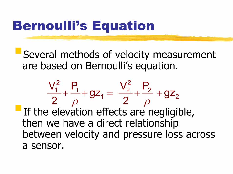
Several methods of velocity measurement are based on Bernoulli’s equation.

If the elevation effects are negligible, then we have a direct relationship between velocity and pressure loss across a sensor.

22

22

1

21 gzP

2VgzP

2V

++=++ρρ

1

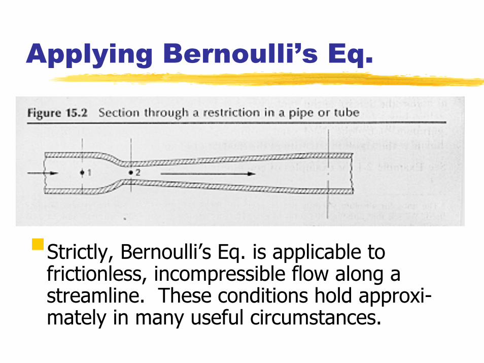
Applying Bernoulli’s Eq.

Strictly, Bernoulli’s Eq. is applicable to frictionless, incompressible flow along a streamline. These conditions hold approxi-mately in many useful circumstances.

Pitot Tubes

A pitot tube is used to measure the static and stagnation pressures of a flowing fluid, which in turn can be related to the local velocity by direct application of the Bernoulli Equation:

( )12

22statstag

21 zzg

2VPP

2V

−++−

=ρ

V2 = 0 because flow is stopped

∆z = 0 because no height change

Pitot Tube (Cont’d)Rearranging this relationship:

A pitot probe yields a “local” velocity.Several measurements are averaged to get volumetric flow rate from the measured V’s. Velocities should be weighted according to the flow area that they represent.

ρstatstag

1PP

V−

⋅= 2

PitotTube

Obstruction Meters

To get volumetric flow rate (Q) of the entire tube with a single measurement of ∆P, obstruction meters are used.Obstruction meters are based roughly on the Bernoulli principle, but with correction to account for non-ideal flow.Three common obstruction meters include: a) venturi, b) flow nozzle and c) orifice meters.

Modifying Bernoulli’s Eq...

Assuming constant z and A1 ≠ A2, and noting that V1⋅A1 = V2 ⋅A2, the Bernoulli Eq. can be rewritten as:

22

22

1

21 gzP

2VgzP

2V

++=++ρρ

1

( )( )

ρ21

21

22

2PP2

AA1

1V −

−=

Modifying Bernoulli (Cont’d)

Define the velocity of approach factor, M:

Noting that volume flow rate is Q = V2⋅A2:

( )2122 AA1

1M−

=

( )ρ

212

PP2AMQ −⋅⋅=

Obstruction Meter Correction

Bernoulli’s equation, assumes ideal flow, such as no friction, no compressible flow.Flow rate predicted from Bernoulli Eq. is the “ideal” flow rate.A friction correction factor, called the “discharge coefficient” C, is defined as:

C = Qactual/Qideal

If C is known, the ideal flow rate can be corrected to actual flow rate.

Compressible Flow Correction

For compressible flow, a correction factor called the expansion factor, Y, is used.All obstruction meters, then, are covered by the “YMCA” equation:

Y < 1 if ∆P/P1 > 0.02 or so.

Y = 1 for incompressible fluids (including allliquids!)

( )ρ

212

PP2ACMYQ −⋅⋅⋅⋅=

Obstruction MetersObstruction meter measurement consists of measuring ∆P, determining Y and C, then applying the YMCA equation.Mass flow rate is:Y and C vary with meter type, geometry, flow rate and (for Y) gas composition.Various charts and equations are available to determine Y and C for meters built to strict specifications (e.g., ASME).

Qm 1 ⋅= ρ&

Venturi Schematic

D d

For all obstruction meters:

β = d/D

FlowNozzle

Schematic

D d

Orifice Schematic

Relative Merits of the Venturi, Nozzle and OrificeVenturi:

Advantages:High accuracyGood pressure recoveryResistance to abrasion

DisadvantagesMore difficult to manufactureMore expensive than nozzle or orificeScaling lowers accuracy more than orifice

Relative Merits (Cont’d)Flow Nozzles:

Advantages:Good accuracyGood pressure recovery (but < venturi)More compact and cheaper than venturi

DisadvantagesMore difficult to install properlyMore expensive than orificeScaling lowers accuracy more than orifice

Relative Merits (Cont’d)Orifices:

Advantages:Easy to install (between flanges)easy to change β (substituting plates)relatively inexpensive

DisadvantagesHigh permanent pressure lossSusceptible to wear from particulatesCan be damaged by pressure transients