Fluid Dynamics - Educating Global Leadersmaynesrd/classes/me412/Boundary Layer.pdf · Fluid...
21
Fluid Dynamics CAx Tutorial: Boundary Layer Growth Basic Tutorial #1 Deryl O. Snyder C. Greg Jensen Brigham Young University Provo, UT 84602 Special thanks to: PACE, Fluent, UGS Solutions, Altair Engineering; and to the following students who assisted in the creation of the Fluid Dynamics tutorials: Leslie Tanner, Cole Yarrington, Stephen McQuay, Curtis Rands, and Curtis Memory.
Transcript of Fluid Dynamics - Educating Global Leadersmaynesrd/classes/me412/Boundary Layer.pdf · Fluid...

Fluid Dynamics
CAx Tutorial: Boundary Layer Growth
Basic Tutorial #1
Deryl O. SnyderC. Greg Jensen
Brigham Young UniversityProvo, UT 84602
Special thanks to:
PACE, Fluent, UGS Solutions, Altair Engineering;
and to the following students who assisted in the creation of the Fluid Dynamics tutorials:
Leslie Tanner, Cole Yarrington, Stephen McQuay, Curtis Rands, and Curtis Memory.


3
Boundary Layer Growth
2D FlowIn this tutorial, Gambit® is used to create and mesh the geometry. Once preprocessingis complete, FLUENT will be used to solve the flow problem. Fluent will then be usedto view velocity vectors and contours.
This basic 2D tutorial should prepare you to model, mesh, define and analyze morecomplex fluid flow problems.
The methods expressed in these tutorials represent just one approach to modeling, defining andsolving 2D problems. Our goal is the education of students in the use of CAx tools for model-ing, constraining and solving fluids application problems. Other techniques and methods will beused and introduced in subsequent tutorials.

4
Boundary Layer Growth
Creating GeometryBegin the problem by creating geometry inGambit.
The Gambit standard display should beopen.
Meshes are generated in Gambit by follow-ing left to right the menu icons located inthe top right of the display window.
Create a rectangle as the computationaldomain.
Operation > Geometry > Face >Create RealRectangular FaceNote: Icons with a red arrow have a pull down menu. Toactivate the pull down menu select the icon with MB3.
Set the Width to be 300 and the Height tobe 400.
Next to Direction, select +X +Y, to place thebottom left corner at the origin.
Note: To fit the geometry to the screen in Gambit, simplyselect the top left icon from the Global Control Menu onthe bottom right of the display window.
If problems are encountered in creating thegeometry, the geometry can be loaded from thefile “Wall_Geometry.dbs”.

5
Boundary Layer Growth
Meshing GeometryNow mesh the rectangular face.
Operation > Mesh > Edge > Mesh Edges
The Mesh Edges window should appear.
When a field is highlighted, entities can beselected from the graphics window. Toselect an entity from the graphics window,hold down the Shift key, and select theentity with MB1.
If the selected edge is the wrong one, dif-ferent entities can be chosen if the shift keyis still depressed. With the shift key stilldepressed, select MB2, and different enti-ties in the graphics window will be high-lighted. Releasing the Shift key will selectthe entity.
Select the left vertical edge. (Use the shiftselect technique in the graphics window.)If the red arrow on the edge is not pointingup, select Reverse.
There are two ways to specify node spac-ing, by interval size, or by interval count.
Under Spacing, select Interval Count fromthe drop down menu.
Enter 100 in the blank field under Spacing.
Next to Type select First Length, and thenenter .1 next to Length.
Select Apply.
Nodes have been clustered close to the bot-tom wall in order to resolve the velocitygradients that are expected next to the wall.
The edge mesh should appear as it does tothe right.

6
Boundary Layer Growth
Meshing GeometrySelect the right vertical edge.
Repeat the previous steps to mesh theedge.Note: Both edges can be meshed at the same time, butcare must be taken to ensure that both arrows are point-ing up. You must select one edge, select Reverse, andthen select the other edge.
Select the Top edge and the Bottom edge.
Now specify the node spacing by IntervalSize.
Make sure that the Apply box next toGrading is unchecked.
Enter 6 next to Interval Size.
Select Apply.

7
Boundary Layer Growth
Meshing GeometryNow mesh the rectangular face.
Operation > Mesh > Face > Mesh Faces
Select the rectangular face.
All fields should be left at their default val-ues.
With Quad selected in the Elements pulldown menu, the domain will be meshedwith quadrilateral elements.
With Map selected form the Type pulldown menu, the meshes will be generatedparallel to the edges.
Select Apply.
The mesh should resemble the one shownto the right.
If problems are encountered in meshing geome-try, the meshed geometry can be loaded from thefile “Wall_Meshed.dbs”.

8
Boundary Layer Growth
Boundary ConditionsThe next task is to specify the boundaryconditions.
The first step is to specify which solverwill be used.
Solver > Fluent 5/6
Next, bring up the Specify BoundaryTypes window by selecting the followingicons: Operation > Zones > Specify BoundaryTypes
From the pull down menu under Entity,select Edges.
Select the left edge.
Next to name type Inlet.
Under Type select Velocity_Inlet.
Select Apply.
Select the bottom edge.
Next to Name type Wall.
Under Type select Wall.
Select Apply.

9
Boundary Layer Growth
Boundary ConditionsSelect the top edge.
Next to Name type Top.
Under Type select Symmetry.
Select Apply.
Select the right edge.
Next to Name type Out.
Select Apply.
Under Type select Outflow.
The Specify Boundary Types windowshould resemble the one shown to theright.
If problems are encountered in specifyingboundary conditions, the completed mesh withboundary conditions specified can be loadedfrom the file “Wall_Complete.dbs”.

10
Boundary Layer Growth
Exporting the MeshExport the mesh
File > Export > Mesh
Make sure the Export 2d (X-Y mesh) box isselected.
Select Browse... to choose the saving direc-tory.
Export the mesh as Wall.msh.
Also save the Gambit file.
File > Save as...
Browse as before.
Select Accept.
Exit out of Gambit.

11
Boundary Layer Growth
Starting in FluentOpen Fluent. A dialog box should appear
Select 2d
Select Run
The following window should appear
This is the FLUENT user interface. Mosttasks are completed using the menus acrossthe top. The menus are designed to guideyou through the analysis in an orderlyfashion, going from top to bottom througheach menu, and left to right across themenu bar.
Text commands can also be used in thecommand window.

12
Boundary Layer Growth
Defining the ProblemStart by importing the mesh created inGambit.
File > Read > Case...A browse window should appear.
Locate Wall.msh and select OK.
FLUENT will read in the geometry andmesh you created. If there are problemsreading the mesh, return to the beginningof the tutorial and make sure you followthe steps carefully. If there are no problemsthe command window should state“Done”.
Now check the grid for errors.
Grid > Check
Any errors will be listed, otherwise thecommand window should again state“Done”.
Set the scale of the grid. To do thisGrid > Scale...
The scale grid window should appear.
From the pull down menu next to GridWas Created In select mm.
Select Scale
The values of Xmax and Ymax shouldchange to .3 and .4, respectively.
Select Close.
13
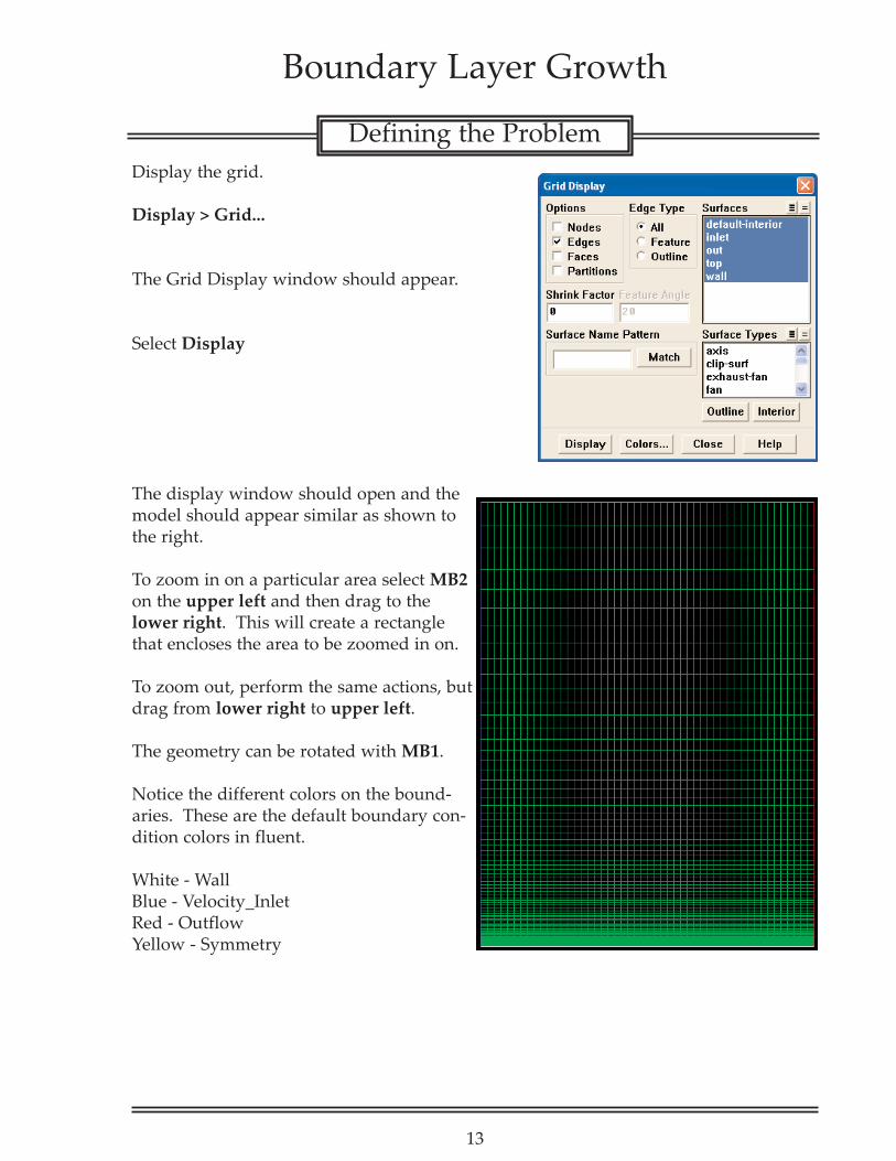
Boundary Layer Growth
Defining the ProblemDisplay the grid.
Display > Grid...
The Grid Display window should appear.
Select Display
The display window should open and themodel should appear similar as shown tothe right.
To zoom in on a particular area select MB2on the upper left and then drag to thelower right. This will create a rectanglethat encloses the area to be zoomed in on.
To zoom out, perform the same actions, butdrag from lower right to upper left.
The geometry can be rotated with MB1.
Notice the different colors on the bound-aries. These are the default boundary con-dition colors in fluent.
White - WallBlue - Velocity_InletRed - OutflowYellow - Symmetry

14
Boundary Layer Growth
Defining the ProblemDefine the type of solver as shown to theright.Define > Models > Solver...
The default implicit segregated solver isappropriate for this laminar, incompress-ible flow problem. Verify that the defaultoptions are selected as shown on the right
Select OK
Next we need to set up the viscous model.Define > Models > Viscous...
Select Laminar
Select OK
Now specify a viscous fluid for the prob-lem. To do this:Define > Materials...
The Materials window should appear

15
Boundary Layer Growth
Defining the ProblemChoose a viscous fluid by selectingDatabase...
Under Fluid Materials select glycerin(c3h8o3).
Select Copy then Close.
Selecting Copy brings the fluid into theworking database, and allows us to changethe properties, and assign the fluid as theworking fluid.
In the following steps the glycerin will bespecified as the working fluid.
In the Materials window selectChange/Create then Close.

16
Boundary Layer Growth
Defining the ProblemSet the Boundary Condition parameters forthe problem.
Define > Boundary Conditions...
The default values are sufficient for allboundaries except for fluid and Inlet.
Select fluid from the Zone list, then fluidunder Type.
Select Set...
Select glycerin from the Material Namedrop down menu.
Select OK.
In the Boundary Conditions Window,select inlet under Zone, and velocity_inletunder Type.
Select Set...
Next to Velocity Magnitude enter 0.5.
Select OK.
Select Close on the Boundary ConditionsWindow.

17
Boundary Layer Growth
Defining the ProblemNext set the solution control parameters.Solve > Controls > Solution...
Change the Under-Relaxation Factor forPressure from 0.3 to 0.9
Note: This change above can be done because the SIM-PLEC discretization method will be used for the pres-sure-velocity coupling.
Under Discretization change the switchnext to Pressure to Second Order.
Change the switch next to Pressure-Velocity Coupling to SIMPLEC.
Change the switch next to Momentum toSecond Order Upwind.
Select OK

18
Boundary Layer Growth
Defining the ProblemNow solve the problem by first initializingthe solution.
Solve > Initialize > Initialize...
The Solution Initialization window shouldappear.
From the drop down menu belowCompute From select Inlet.
Select Init then close
Now set the monitors to plot the residuals.To do this
Solve > Monitors > Residual...
The Residual Monitors window shouldappear.
Put a check next to Plot.
Uncheck the 3 boxes under CheckConvergence.
If the Check Convergence boxes arechecked, iterations will halt once all of theconvergence criteria are met.
Leaving them unchecked allows the opera-tor to monitor them manually, and stopiterating when the solution is converged.
Select OK
The model is now ready to be solved.

19
Boundary Layer Growth
Solving the ProblemTo solve the model:Solve > Iterate...
The Iterate window should appear.
In the Number of Iterations text box, enter600.
Select Iterate
Fluent solves the problem and the residualplot should appear.
Check the plot to see if the solution is con-verged. Since we unchecked the CheckConvergence, to tell if the solution is con-verging we look for the residuals to taperoff to a slope of zero.
After 600 iterations, the solution is not yetfully converged, but it is sufficient to viewvelocity vectors and contours.
If problems are encountered in setting up thisproblem in fluent, the solved problem can beread in as a “Case and Data” from the file“Wall.cas”.

20
Boundary Layer Growth
Analyzing the ResultsNow view the results.
Display > Vectors
The Vectors window should appear
Under Vectors Of select Velocity
Select Display
The model should be displayed with vec-tors representing the velocities. Theboundary layer can be seen to grow fromthe left side to the right as is expected.
In subsequent tutorials, numerical solu-tions will be compared to analytical solu-tions. In this tutorial, viewing the results isthe main focus.

21
Boundary Layer Growth
Analyzing the ResultsContours are viewed the same way asvelocity vectors.
Display > Contours...
Contours can displayed for many differentvalues.
The default is set to pressure. From theContours Of drop down menu selectVelocity...
Under Options, select Filled, to see filledin contours, otherwise only the contourlines will be displayed.
The Number of Contour levels can also bespecified. For smoother transitionsbetween contours, select a large number.The range is from 1 to 100.
Under Levels enter 100.
Select Display.
The image should resemble the one shownto the right.
In both the vector and contour displaysvalues for specific locations can beobtained by selecting the location withMB3.
When selecting a location with MB3, thevalue is shown on the scale to the left ofthe display, and also in the command win-dow.