Fluent Tutorial 02 Modeling Periodic Flow and Heat Transfer

8/3/2019 Fluent Tutorial 02 Modeling Periodic Flow and Heat Transfer

http://slidepdf.com/reader/full/fluent-tutorial-02-modeling-periodic-flow-and-heat-transfer 1/26

Tutorial 2. Modeling Periodic Flow and Heat Transfer

Introduction

Many industrial applications, such as steam generation in a boiler or air cooling in thecoil of an air conditioner, can be modeled as two-dimensional periodic heat flow. Thistutorial illustrates how to set up and solve a periodic heat transfer problem, given apregenerated mesh.

The system that is modeled is a bank of tubes containing a flowing fluid at one temper-ature that is immersed in a second fluid in cross-flow at a different temperature. Bothfluids are water, and the flow is classified as laminar and steady, with a Reynolds number

of approximately 100. The mass flow rate of the cross-flow is known, and the model isused to predict the flow and temperature fields that result from convective heat transfer.

Due to symmetry of the tube bank and the periodicity of the flow inherent in the tubebank geometry, only a portion of the geometry will be modeled in FLUENT, with sym-metry applied to the outer boundaries. The resulting mesh consists of a periodic modulewith symmetry. In the tutorial, the inflow boundary will be redefined as a periodic zone,and the outflow boundary defined as its shadow.

In this tutorial you will learn how to:

• Create periodic zones.

• Define a specified periodic mass flow rate.

• Model periodic heat transfer with specified temperature boundary conditions.

• Calculate a solution using the segregated solver.

• Plot temperature profiles on specified isosurfaces.

Prerequisites

This tutorial assumes that you are familiar with the menu structure in FLUENT and thatyou have completed Tutorial 1 . Some steps in the setup and solution procedure will notbe shown explicitly.

c Fluent Inc. January 11, 2005 2-1

http://tut01.pdf/



Modeling Periodic Flow and Heat Transfer

Problem Description

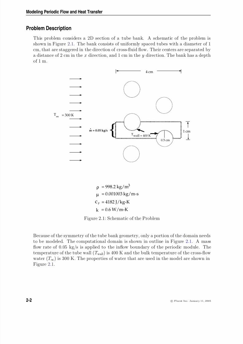
This problem considers a 2D section of a tube bank. A schematic of the problem isshown in Figure 2.1. The bank consists of uniformly spaced tubes with a diameter of 1cm, that are staggered in the direction of cross-fluid flow. Their centers are separated bya distance of 2 cm in the x direction, and 1 cm in the y direction. The bank has a depth

of 1 m.

1 cm

Τ∞ = 300 K

4 cm

0.5 cm

Τwall = 400 K{m = 0.05 kg/s⋅

ρ = 998.2 kg/m3

= 0.001003 kg/m-sµ

= 4182 J/kg-K

= 0.6 W/m-K

c p

k

Figure 2.1: Schematic of the Problem

Because of the symmetry of the tube bank geometry, only a portion of the domain needs

to be modeled. The computational domain is shown in outline in Figure 2.1. A massflow rate of 0.05 kg/s is applied to the inflow boundary of the periodic module. Thetemperature of the tube wall (T wall) is 400 K and the bulk temperature of the cross-flowwater (T ∞) is 300 K. The properties of water that are used in the model are shown inFigure 2.1.

2-2 c Fluent Inc. January 11, 2005




Setup and Solution

Preparation

1. Download periodic_flow_heat.zip from the Fluent Inc. User Services Centeror copy it from the FLUENT documentation CD to your working directory (as

described in Tutorial 1).

2. Unzip periodic_flow_heat.zip .

tubebank.msh can be found in the /periodic flow heat folder created after un-zipping the file.

3. Start the 2D version of FLUENT.

Step 1: Grid

1. Read the mesh file, tubebank.msh.

File −→ Read −→Case...

2. Check the grid.

Grid −→Check

FLUENT will perform various checks on the mesh and report the progress in theconsole window. Make sure that the minimum volume reported is a positive num-ber.

3. Scale the grid.

Grid −→Scale...

(a) Under Units Conversion, select cm (centimeters) from the drop-down list tocomplete the phrase Grid Was Created In cm.

(b) Click Scale to scale the grid and close the panel.


http://-/?-




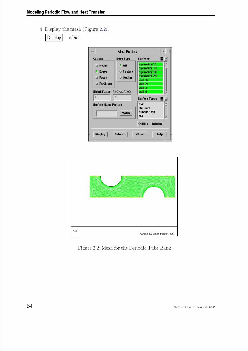
4. Display the mesh (Figure 2.2).

Display −→Grid...

GridFLUENT 6.2 (2d, segregated, lam)

Figure 2.2: Mesh for the Periodic Tube Bank





Quadrilateral cells are used in the regions surrounding the tube walls, and triangular cells are used for the rest of the domain, resulting in a hybrid mesh (See Figure 2.2 ).The quadrilateral cells provide better resolution of the viscous gradients near thetube walls. The remainder of the computational domain is conveniently fil led with triangular cells.

Extra: Right-click on one of the boundaries in the graphics window to check which zone number corresponds to the boundary. The zone number, name, and typewill be printed in the FLUENT console window. This feature is especially useful when there are several zones of the same type and you want to distinguish between them.

5. Create the periodic zone.

The inflow ( wall-9) and outflow ( wall-12) boundaries currently defined as wall zonesneed to be redefined as periodic. Redefine the wall-9 boundary as translationally periodic zone, and wall-12 as periodic shadow of wall-9.

(a) In the console window, enter the inputs shown in boxes in the following dialog.

Hint: Press <Enter > to get the command prompt ( >).

grid/modify-zones/make-periodic

Periodic zone [()] 9

Shadow zone [()] 12

Rotational periodic? (if no, translational) [yes] no

Create periodic zones? [yes] yes

Auto detect translation vector? [yes] yes

computed translation deltas: 0.040000 0.000000

all 26 faces matched for zones 9 and 12.

zone 12 deleted

created periodic zones.





Step 2: Models

1. Keep the default solver settings.

Define −→ Models −→Solver...

2. Enable heat transfer by activating the energy equation.

Define −→ Models −→Energy...





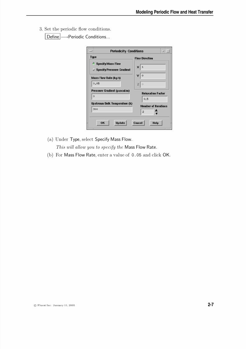
3. Set the periodic flow conditions.

Define −→Periodic Conditions...

(a) Under Type, select Specify Mass Flow.

This will allow you to specify the Mass Flow Rate.

(b) For Mass Flow Rate, enter a value of 0.05 and click OK.





Step 3: Materials

Add liquid water to the list of fluid materials by copying it from the materials database.

1. Copy the properties of liquid water from the database.

Define −→Materials...(a) Click on the Fluent Database... button.

This will open the Fluent Database Materials panel.

(b) Select water-liquid (h2o<l>) from the Fluent Fluid Materials list.

This will display the default settings for water-liquid. You will have to scroll down the Fluent Fluid Materials list to see the entries.

(c) Click Copy and Close the panel.

The Materials panel will now display the copied information of water.





Step 4: Boundary Conditions

Define −→Boundary Conditions...

1. Set the conditions for fluid-16.

(a) In the Material Name drop-down list, select water-liquid





2. Set the boundary conditions for wall-21.

This is the bottom wall of the left tube in the periodic module shown in Figure 2.1.

(a) Change Zone Name to wall-bottom.

(b) Under Thermal Conditions, select Temperature.

(c) Set the Temperature to 400 K.





3. Set the boundary conditions for wall-3.

This is the top wall of the right tube in the periodic module shown in Figure 2.1.

(a) Change the Zone Name to wall-top.

(b) Under Thermal Conditions, select Temperature.

(c) Set the Temperature to 400 K.

(d) Click OK to close the panel.





Step 5: Solution

1. Set the solution parameters.

Solve −→ Controls −→Solution...

(a) Set the Under-Relaxation Factor for Energy to 0.9.

Hint: Scroll down the Under-Relaxation Factors list to see Energy.

(b) Under Discretization, select Second Order Upwind for Momentum and Energy.





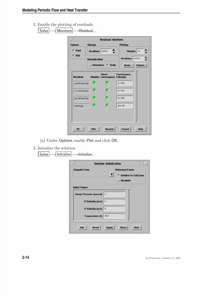
2. Enable the plotting of residuals.

Solve −→ Monitors −→Residual...

(a) Under Options, enable Plot and click OK.

3. Initialize the solution.

Solve −→ Initialize −→Initialize...





(a) Under Initial Values, check that the value for Temperature is set to 300 K.

(b) Click Init and Close the panel.

4. Save the case file, tubebank.cas.

File −→ Write −→Case...

5. Start the calculation by requesting 350 iterations.

Solve −→Iterate...

(a) Set the Number of Iterations to 350.

(b) Click Iterate.

The energy residual curve begins to flatten out after about 350 iterations. For thesolution to converge, you need to reduce the under-relaxation factor for energy.

6. Change the Under-Relaxation Factor for Energy to 0.6.

Solve −→ Controls −→Solution...

7. Continue the calculation by requesting another 300 iterations.

Solve −→Iterate...

After restarting the calculation, you will see an initial dip in the plot of the energy residual as a result of reduction in the under-relaxation factor. The solution will converge in a total of approximately 580 iterations.

8. Save the case and data files, tubebank.cas and tubebank.dat.

File−→

Write−→

Case & Data...





Step 6: Postprocessing

1. Display filled contours of static pressure (Figure 2.3).

Display −→Contours...

(a) Under Options, select Filled.

(b) In the Contours of drop-down list, select Pressure... and Static Pressure.

(c) Click Display (Figure 2.3).

2. Change the view to mirror the display across the symmetry planes (Figure 2.4).

Display −→Views...





Contours of Static Pressure (pascal)FLUENT 6.2 (2d, segregated, lam)

8.18e-02

7.55e-02

6.92e-02

6.28e-02

5.65e-02

5.02e-02

4.38e-02

3.75e-02

3.12e-02

2.48e-02

1.85e-02

1.22e-02

5.82e-03

-5.13e-04

-6.85e-03

-1.32e-02

-1.95e-02

-2.59e-02

-3.22e-02

-3.85e-02

-4.49e-02

Figure 2.3: Contours of Static Pressure

(a) Under Mirror Planes, select all of the symmetry zones by clicking the shadedicon at the right side.

Note: There are four symmetry zones in the Mirror Planes list because the

top and bottom symmetry planes in the domain are each comprised of two symmetry zones, one on each side of the tube. It is also possible togenerate the same display shown in Figure 2.4 by selecting just one of thesymmetry zones on the top symmetry plane, and one on the bottom.

(b) Click Apply and Close the panel.





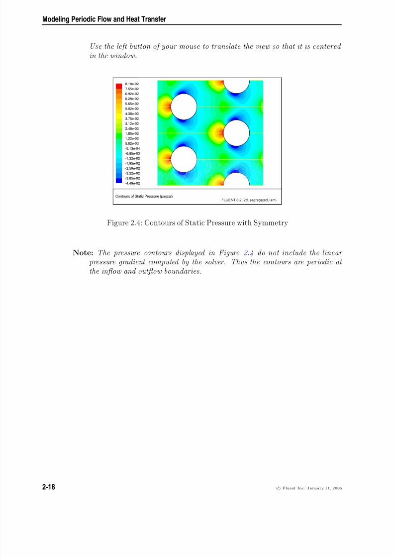
Use the left button of your mouse to translate the view so that it is centered in the window.

Contours of Static Pressure (pascal)FLUENT 6.2 (2d, segregated, lam)

8.18e-02

7.55e-02

6.92e-02

6.28e-02

5.65e-02

5.02e-02

4.38e-02

3.75e-02

3.12e-02

2.48e-02

1.85e-02

1.22e-02

5.82e-03

-5.13e-04

-6.85e-03

-1.32e-02

-1.95e-02

-2.59e-02

-3.22e-02

-3.85e-02

-4.49e-02

Figure 2.4: Contours of Static Pressure with Symmetry

Note: The pressure contours displayed in Figure 2.4 do not include the linear pressure gradient computed by the solver. Thus the contours are periodic at the inflow and outflow boundaries.





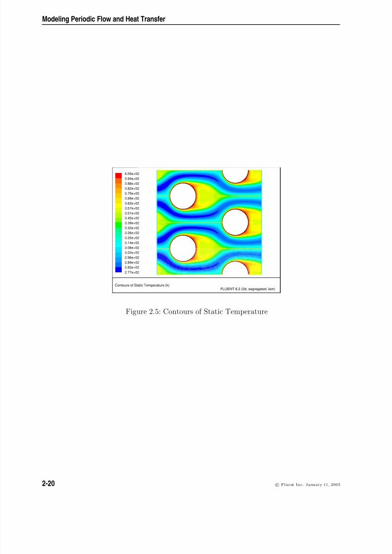
3. Display filled contours of static temperature (Figure 2.5).

Display −→Contours...

(a) In the Contours of drop-down list, select Temperature... and Static Temperatureand click Display (Figure 2.5).

The contours reveal the temperature increase in the fluid due to heat transfer from the tubes. The hotter fluid is confined to the near-wall and wake regions, while a narrow stream of cooler fluid is convected through the tube bank.





Contours of Static Temperature (k)FLUENT 6.2 (2d, segregated, lam)

4.00e+02

3.94e+02

3.88e+02

3.82e+02

3.75e+023.69e+02

3.63e+02

3.57e+02

3.51e+02

3.45e+02

3.39e+02

3.32e+02

3.26e+02

3.20e+02

3.14e+02

3.08e+02

3.02e+02

2.96e+02

2.89e+02

2.83e+02

2.77e+02

Figure 2.5: Contours of Static Temperature





4. Display the velocity vectors (Figure 2.6).

Display −→Vectors...

(a) In the Color By drop-down list, select Velocity... and Velocity Magnitude.

(b) Set the Scale to 2 and click Display.

This will enlarge the displayed vectors that are displayed, making it easier toview the flow patterns.

(c) Zoom in on the upper right portion of the left tube using your middle mousebutton, to get the display shown in Figure 2.6.

This zoomed-in view of the velocity vector plot clearly shows the recirculating flow behind the tube and the boundary layer development along the tube surface.

5. Plot the temperature profiles at three cross sections of the tube bank.

(a) Create an isosurface on the periodic tube bank at x = 0.01 m (through thefirst tube).

Create a surface of constant x coordinate for each the cross sections, x = 0.01,0.02, and 0.03 m. These isosurfaces correspond to the vertical cross sections





Velocity Vectors Colored By Velocity Magnitude (m/s)FLUENT 6.2 (2d, segregated, lam)

1.31e-02

1.25e-02

1.18e-02

1.12e-02

1.05e-02

9.85e-03

9.19e-03

8.53e-03

7.88e-03

7.22e-03

6.56e-03

5.91e-03

5.25e-03

4.60e-03

3.94e-03

3.28e-03

2.63e-03

1.97e-03

1.31e-03

6.58e-04

1.93e-06

Figure 2.6: Velocity Vectors

through the first tube, halfway between the two tubes, and through the second tube.

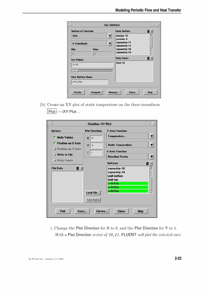
Surface −→Iso-Surface...

i. In the Surface of Constant drop-down lists, select Grid... and X-Coordinate.

ii. Enter x=0.01m under New Surface Name.

iii. Enter 0.01 for Iso-Values and click Create.

iv. Follow the same procedure to create surfaces at x = 0.02 m (halfwaybetween the two tubes) and x = 0.03 m (through the middle of the secondtube).





(b) Create an XY plot of static temperature on the three isosurfaces.

Plot −→XY Plot...

i. Change the Plot Direction for X to 0, and the Plot Direction for Y to 1.

With a Plot Direction vector of (0,1), FLUENT will plot the selected vari-





able as a function of y. Since you are plotting the temperature profile on cross sections of constant x, the temperature varies with the y direction.

ii. Select Temperature... and Static Temperature in the Y-Axis Function drop-down lists.

iii. Scroll down the Surfaces list and select x=0.01m, x=0.02m, and x=0.03m.

iv. Click Curves....

This will open the Curves - Solution XY Plot panel, used to define different plot styles for the different plot curves.

A. Select + in the Symbol drop-down list.

B. Click Apply.

This assigns the + symbol to the x = 0.01 m curve.

C. Increase the Curve # to 1 to define the style for the x = 0.02 m curve.D. Select x in the Symbol drop-down list.

E. Set the value of Size to 0.5.

F. Click Apply and close the panel.

Since you did not change the curve style for the x = 0.03 m curve,the default symbol will be used.

v. In the Solution XY Plot panel, click Plot.





Static Temperature

FLUENT 6.2 (2d, segregated, lam)

Position (m)

(k)Temperature

Static

0.010.0090.0080.0070.0060.0050.0040.0030.0020.0010

4.00e+02

3.80e+02

3.60e+02

3.40e+02

3.20e+02

3.00e+02

2.80e+02

2.60e+02

x=0.03mx=0.02mx=0.01m

Figure 2.7: Static Temperature at x=0.01, 0.02, and 0.03 m





Summary

In this tutorial, periodic flow and heat transfer in a staggered tube bank were modeledin FLUENT. The model was set up assuming a known mass flow through the tube bankand constant wall temperatures. Due to the periodic nature of the flow and symmetry of the geometry, only a small piece of the full geometry was modeled. In addition, the tube

bank configuration lent itself to the use of a hybrid mesh with quadrilateral cells aroundthe tubes and triangles elsewhere.

The Periodicity Conditions panel makes it easy to run this type of model over a varietyof operating conditions. For example, different flow rates (and hence different Reynoldsnumbers) can be studied, or a different inlet bulk temperature can be imposed. Theresulting solution can then be examined to extract the pressure drop per tube row andoverall Nusselt number for a range of Reynolds numbers.

Fluent Tutorial 02 Modeling Periodic Flow and Heat Transfer

Documents

Transcript of Fluent Tutorial 02 Modeling Periodic Flow and Heat Transfer