HYDROXYL TAGGING VELOCIMETRY (HTV) IN HIGHLY ACCELERATED

FLOWS

By

Amber Nicole Perkins

Thesis

Submitted to the Faculty of the

Graduate School of Vanderbilt University

in partial fulfillment of the requirements

for the degree of

MASTER OF SCIENCE

in

Mechanical Engineering

December, 2011

Nashville, Tennessee

Approved:

Joseph A. Wehrmeyer

Don G. Walker

Robert W. Pitz

ii

ACKNOWLEDGEMENTS

This work was supported by Arnold Engineering Development Center under

contract No. F40600-03-D-001. I would like to thank Dr. Joseph Wehrmeyer and Dr.

Robert Pitz for their assistance and support. I would also like to thank Marc C. Ramsey

for his efforts. Last, but certainly not least, I would like to thank my mother Joy Guthrie

for supporting me and helping me to see the end in the beginning.

iii

TABLE OF CONTENTS

Page

ACKNOWLEDGEMENTS ............................................................................................ II

LIST OF TABLES .......................................................................................................... IV

LIST OF FIGURES ......................................................................................................... V

INTRODUCTION............................................................................................................. 1

1.1 LASER DIAGNOSTIC TECHNIQUES TO MEASURE GAS VELOCITY ............................. 1

1.2 PREVIOUS HTV WORK ............................................................................................. 4

1.3 HTV IN TURBOJET ENGINE EXHAUST ....................................................................... 4

1.4 HTV IN SHOCK TUBE FLOW ...................................................................................... 5

HYDROXYL TAGGING VELOCIMETRY APPLIED TO JET ENGINE ............... 5

2.1 ENGINE FACILITY ..................................................................................................... 5

2.2 EXPERIMENTAL SYSTEM .......................................................................................... 6

2.3 TEST CONDITIONS .................................................................................................... 8

2.4 POST-PROCESSING .................................................................................................. 12

2.4.1 Uncertainty ................................................................................................... 18

2.5 DUAL-PULSE AND SINGLE IMAGE METHOD COMPARISON ....................................... 19

2.6 CONCLUSION .......................................................................................................... 22

INVESTIGATION OF A BOW SHOCK USING HTV .............................................. 23

3.1 INTRODUCTION ...................................................................................................... 23

3.2 EXPERIMENTAL SYSTEM ........................................................................................ 24

3.3 EXPERIMENTAL RESULTS ....................................................................................... 30

3.3.1 Blunt Nose Model .......................................................................................... 32

3.3.2 Cone Model ................................................................................................... 36

3.4 CONCLUSION .......................................................................................................... 39

REFERENCES ................................................................................................................ 40

iv

LIST OF TABLES

Table Page

1. Engine test conditions, delay times, and average centerline displacements using the

dual-pulse method ............................................................................................................. 10

2. Image pairs and intersection ......................................................................................... 16

3. Measured and calculated shock speed. The calculated shock speed is determined from

P4/P1 using Equation 4 and 5. The pressure ratio P2/P1 is calculated from the measured

shock speed using Equation 6. * Pressure, P4 ,for test condition 6 could not be accurately

determined......................................................................................................................... 30

v

LIST OF FIGURES

Figure Page

1. (a) Schematic showing hydroxyl production (193-nm), excitation (282-nm), and

imaging (b) Schematic showing grid tracking process. ...................................................... 3

2. Schematic showing engine exhaust, tag lines, and camera field of view (with the

interrogation area drawn to scale on left and an expanded view on the right). .................. 7

3. Timing schematic for dual-pulse imaging. ..................................................................... 8

4. HTV dual-pulse images (41.6 mm x 41.6 mm) at each throttle condition [undisplaced

(0 µs) and displaced (3-9 µs)]. .......................................................................................... 11

5. (a) Special correlation software depiction showing source and roam windows (b)

Displacement vector determination .................................................................................. 13

6. SNR definition. (From a vertical line out at x=21.8 mm) To moderate the influence of

outliers (such as faulty pixels), N is estimated by 6 standard deviations, an interval which

contains about 99% of normally distributed noise ............................................................ 14

7. Fuel signal derived from 193-nm laser-induced fluorescence ...................................... 15

8. Displaced HTV image (3 µs time delay) where read sheet is out of plane ................... 15

9. HTV derived centerline velocity vectors for engine setting 3 at the nozzle exit. ......... 17

10. HTV derived centerline velocity vectors for engine setting 3 superimposed on an

undisplaced image (a) velocity magnitude and (b) expanded view of velocity magnitude

........................................................................................................................................... 17

11. Measured velocity derived from HTV data. ............................................................... 18

12. Comparison of dual-pulse and single-image method velocity deviation from the mean

for J-85 jet engine. ............................................................................................................ 21

13. Velocity uncertainty from the mean derived from HTV data, where dx is the average

centerline displacement from Table 1 ............................................................................... 21

14. Side-view of shock tube. Pressure transducers K4 and K5 are used to determine shock

speed. Laser beams are directed through the side of the test section window (100 mm x

20 mm). ............................................................................................................................. 24

vi

15. Test articles for experiment. Cone model (top) and blunt nose model (bottom). Each

test article is attached to a 110 mm sting. ......................................................................... 25

16. Laser pulse and camera gate timing from typical shock tube shot ............................. 27

17. Pressure transducer scope traces (a) K4 scope trace to indicate incident and reflected

shock location (b) K4 and K5 scope trace. K4 and K5 are used to determine incident

shock speed ....................................................................................................................... 28

18. Measured and calculated shock speed comparison ..................................................... 29

19. Undisplaced (a) and displaced image (b) pair for shot 3 for the blunt nose model with

a measured free stream velocity of 1690 m/s. Image area: 29.5 mm x 29.5 mm. ............ 33

20. Velocity vectors for blunt nose model shot 3 superimposed on the displaced image.

Image area: 29.5 mm x 29.5 mm. ..................................................................................... 33

21. Velocity line out of blunt nose model image for shot 3 at y=7 mm. The circled

numbers indicate the crossing location for each measurement. Image area: 29.5 mm x

29.5 mm. ........................................................................................................................... 34

22. Measured and calculated velocity downstream of shock for blunt nose model. ........ 35

23. Standoff distance, Δd, from the stagnation point of the blunt nose model for the three

shock tube shots. ............................................................................................................... 35

24. Undisplaced and displaced image pair for shot 6 for the cone model with a measured

shock speed of 1660 m/s. Image area: 29.5 mm x 29.5 mm. ............................................ 37

25. Velocity vectors for cone model shot 6 superimposed on the displaced image. Image

area: 29.5 mm x 29.5 mm. ................................................................................................ 37

26. Measured and calculated velocity downstream of shock for the cone model ............. 38

27. Measured and calculated wave angle for the cone model ........................................... 38

1

CHAPTER I

INTRODUCTION

1.1 Laser Diagnostic Techniques to Measure Gas Velocity

Non-intrusive velocity measurements in gas flowfields have recently been

performed with molecular tags that do not require the addition of particles to the gas flow

(Alexander 2008; Blandford 2008; Ismailov 2006; Mittal 2009). An alternative to these

molecular velocity measurements are particle methods such as particle velocimetry (PIV)

where particle displacements are measured and related to the gas velocity (Fajardo 2009;

Timmerman 2009). In PIV, particles are seeded uniformly into the gas and the particle

must closely follow the gas flow (Ismailov 2006). PIV is undesirable in gas flows where

the flow is highly accelerated and swirled such that the particle velocity differs from the

gas velocity. In jet engine test facilities, the addition of particles is prohibited and the

rapid acceleration of the gas through the nozzle requires an alternative method. Thus

molecular tagging velocimetry is a preferable alternative to particle methods to measure

velocity non-intrusively in jet engine exhausts.

Molecular tagging velocimetry (MTV) is sometimes used to characterize fluid

flows (Alexander 2008; Blandford 2008; Ismailov 2006; Mittal 2009; Sitjsema 2002).

MTV has been employed by several researchers to examine in-cylinder cold flow

characteristics of optical engines by premixing biacetyl into a nitrogen gas flow, exciting

the biacetyl phosphorescence in a grid pattern with a 308 nm XeCl excimer laser, and

tracking the luminance grid to determine the velocity (Mittal 2009; Stier 1999; Ismailov

2006). However, the biacetyl tag method is limited to the study of cold oxygen-free

2

gases due to phosphorescence quenching by oxygen. Another MTV technique applied by

Miles et al. (2000), uses the vibrational excitation of oxygen molecules by Raman

excitation followed by interrogation using laser-induced electronic fluorescence

(RELIEF) to examine the velocity. The application of RELIEF to high-temperature

combustion exhausts is problematic due to the natural presence of vibrationally excited

oxygen that obscures the tagged lines. Grids of NO have been created to measure

velocity by MTV using seeded and unseeded techniques. NO2 can be seeded into a gas

flow and subsequently dissociated to form a grid of NO (Hsu 2009). However, the NO2

gas will rapidly decompose in the high-temperature regions of combustion devices. In

the air photolysis and recombination tracking (APART) method, a focused ArF excimer

laser forms a short tag line (~1 cm) from air in the focal region (Sijtsema 2002).

In Hydroxyl Tagging Velocimetry (HTV), an OH tag is created by dissociating

the water vapor naturally present in the flow thus eliminating the need for insertion of a

molecular species for tagging (Ribarov 2002; Pitz 2000). In addition, the OH tag persists

at high temperature conditions (Wehrmeyer 1999). The HTV technique creates a grid of

hydroxyl radicals (OH) by photodissociation of water vapor via a 193-nm ArF excimer

laser. The H2O photodissociation by the 193-nm laser is a single photon process that can

create long OH tag lines. After creating an OH grid, the grid is imaged at zero time

(undisplaced) and a later time (displaced), as seen in Figure 1. The velocity is calculated

by measuring the individual displacements within the molecular grid and dividing by the

time interval between the writing and reading processes.

3

Figure 1. (a) Schematic showing hydroxyl production (193-nm), excitation (282-nm), and

imaging (b) Schematic showing grid tracking process.

ArF

Pulsed

Laser

Nd:YAG

Pulsed

Laser

282 nm

193 nm

Dye

Laser

UV

Tracker

ICC

D

Cam

era

~3

08 n

m

3-5 µs Delay

H

H

H

H

O

O

(a)

(b)

4

1.2 Previous HTV work

Previously, HTV has been applied to supersonic air flow over a cavity in a

research cell; HTV images were recorded with a signal-to-noise ration (SNR) of ~10 to

obtain instantaneous velocity measurements with a precision of ~1% in the ~680 m/s free

stream (Pitz 2005; Lahr 2010). Applications of HTV to engine test cell environments are

more difficult due to test cell vibrations and reduced light collection at longer light

collection distances. In a previous application of HTV to a J85-GE-5 jet engine exhaust,

velocity measurements were made in the centerline at full throttle conditions yielding a

mean velocity of ~540 m/s and a rms variation of ~5% (Blandford 2008; Alexander

2008). In these previous J85 jet engine tests, the displaced HTV image was

instantaneously measured and compared to an undisplaced HTV image previously

recorded before the engine is fired; consequently, vibration of the optical setup would

contribute to the rms variation measurement (Blandford 2008; Alexander 2008).

1.3 HTV in turbojet engine exhaust

In Chapter II, HTV is applied to a turbojet engine exhaust and images are

recorded with an intensified interline-transfer CCD camera operating in dual-pulse mode.

The dual-pulse feature allows for imaging of the initial and displaced grids in quick

succession to create image pairs for analysis. The engine vibrations cause the camera to

move with respect to the initial grid. This relative movement creates error in determining

the initial placement of the grid, when using a single image camera. The dual pulse

imaging technique is likely to have the advantage of reducing the effects of engine

vibrations on the velocity error.

5

1.4 HTV in shock tube flow

In Chapter III, HTV is applied to a shock tube flow to contribute to previous

measurements taken by Smith et al. (1994) in the same facility. The shock tube study

aims to determine the velocity downstream of the initial shock wave. In conjunction with

pressure transducers placed along the length of the tube to determine shock speed, HTV

images are analyzed using a spatial correlation technique to determine displacements of

the grid intersections and thereby the two-dimensional velocity distribution downstream

of the initial shock wave. These measurements provide a preliminary means for

exploring the possibilities of validating theoretical codes and CFD.

CHAPTER II

HYDROXYL TAGGING VELOCIMETRY APPLIED TO JET ENGINE

2.1 Engine Facility

The HTV measurements were conducted on a General Electric J85-GE-5 turbojet

engine mounted on a portable test stand located at the Propulsion Research Facility at the

University of Tennessee Space Institute in Tullahoma, TN. The J85-GE-5 is a single-

shaft turbojet engine used in the T38 military plane. It is composed of an eight-stage

axial-flow compressor powered by two turbine stages and can produce up to 2,400 lbf of

thrust and 3,600 lbf in afterburner (augmented) mode. The engine is used as a test bed to

develop and evaluate intrusive and non-intrusive instrumentation before they are applied

to larger engines and facilities (Alexander 2008). For the current study, the engine is not

6

tested in augmented mode due to absorption of the tag lines by one or more gas species

(Alexander 2008).

2.2 Experimental System

A tunable 193-nm ArF excimer laser (Lambda Physik COMPex 150-T, 193-194

nm) with output energy of 150 mJ per pulse, 0.2 mrad divergence, and a pulse duration of

20 ns was used to photodissociate the water vapor to produce OH radicals. The ArF laser

was operated in broadband mode at 193.4 nm (0.5 nm bandwidth). The ArF beam, 20

mm high by 10 mm wide, was split via a beam splitter and sent into grid forming optics.

The grid forming optics consist of two sets of optics closely spaced: a 300 mm focal

length cylindrical lens (25 mm x 40 mm) and a stack of eleven cylindrical lenses (20 mm

long x 2 mm wide). Each set of grid optics forms 11 parallel beams with energy of ~2.0

mJ/beam and spacing of about 2 mm. The two sets of 11 beams are crossed at a 24º

angle. A schematic showing the engine exhaust, tag lines, and camera field of view is

shown in Figure 2.

The OH radicals were excited by a Nd:YAG (Continuum Lasers Powerlite 9010)

pumped tunable dye laser with an ultraviolet wavelength extender. The doubled output

of the dye laser is tuned to excite the strong Q1(1) line in the A2Σ

+ (vʹ=1)←X

2Πi (vʹʹ=0)

OH band at a wavelength of 281.997 nm (35461.330 cm-1

). The Q1(1) line was chosen in

order to be able to visualize the OH fluorescence under both cold air and hot combustion

exhaust conditions (Ribarov 2005). The dye laser wavelength and the Q1(1) line position

was determined by fluorescence excitation spectra taken in room air and in a propane

torch as done previously (Pitz 2005; Ribarov 2005). The ~282 nm beam (~7 mJ/pulse)

7

was expanded by a negative cylindrical lens (focal length -150 mm) and focused into a

sheet 25 mm wide by 0.5 mm thick with a 1000 mm focal length spherical lens.

Figure 2. Schematic showing engine exhaust, tag lines, and camera field of view (with

the interrogation area drawn to scale on left and an expanded view on the right).

The images were recorded using an intensified interline CCD dual-pulse camera

(Princeton Instruments PI-MAX II 1024x1024 pixels). The dual-pulse feature takes

advantage of the camera’s ability to acquire a second image, the displaced image, while

the first image, the undisplaced image, is being read out. As soon as the first image is

acquired, it is shifted and held. The second exposure begins and is held in the active area

until the first image is read out. The fluorescence light was collected by a 105 mm focal

length f/4.5 UV Nikon camera lens positioned above the jet engine exhaust at the nozzle

exit. To capture the OH fluorescence near ~305-325 nm and block interfering

background light from the lasers (193-nm, 282-nm), a Schott UG-11 (1 mm thick) filter

and a WG305 (3 mm thick) filter were used in front of the camera lens to create a

Jet Engine

Exhaust

45.7

cm

PLIF

Sheet

y

x

Expanded

Interrogation Area Interrogation Area

41 mm x 41 mm Camera Field of View

42 mm x 42 mm

8

bandpass filter from 305-375 nm. Operating in dual-pulse mode, the camera captures

images in quick succession (minimum separation time of 2 µs): one of the undisplaced

grid and the other of the displaced grid. Figure 3 shows the timing schematic with

respect to the firing of the YAG laser and the two camera gates. The first camera gate

captures the undisplaced grid, while the second camera gate captures the displaced image.

To increase the data acquisition rate during the engine test, the camera pixels were binned

4x4 during the camera read-out process to give a final image with a 256x256 pixel

format. The camera image was calibrated by placing a ruler in the focal plane giving a

factor of 6.16±0.02 pix/mm that is used to determine displacements. The 256x256 pixel

images corresponded to a 41.6 mm x 41.6 mm area in the jet engine exhaust.

Figure 3. Timing schematic for dual-pulse imaging.

2.3 Test Conditions

The HTV measurements were performed to determine the centerline velocities at

the closest access point of the jet engine exhaust. The engine testing was performed for

Nd:YAG Flashlamp Pulse

160 s

Camera Image

Read

Camera Gate 200ns

HTV Tag

Delay 3-9 µs

Ar F Pulse ~20ns

OH

PLIF ~30ns

Camera Gate

200ns

9

six engine conditions ranging from idle to full throttle. In Table 1, the six engine

conditions; delay times between the write and read lasers and the average measured

centerline displacement are shown. Time delays were taken at 0, 3, 5, 7, and 9 µs delays

for each throttle condition. The time delays reported are chosen to keep the grid

displacement less than the grid spacing (~2 mm) to prevent ambiguity in computing the

grid movement. At the higher throttle settings, the delay time was decreased from 9 µs to

3 µs to keep the displacement below 2 mm. With these short time delays (3-9 µs), the

effects of optical vibrations and beam wandering induced by the engine vibrations on the

displacement of the tagged grid over the delay time is eliminated as the equipment

vibrations at 100,000 Hz are negligible.

A harmonic analysis can be performed to verify that optical equipment vibrations

are less than 100,000Hz. Consider an aluminum optic mount attached to a stainless steel

post. The natural frequency of the system, given by

m

kf n

2

1 (1)

where, k is the stiffness and m is the mass of the system. The stiffness is given by

L

EAk o (2)

where, E is the modulus of elasticity, Ao the cross-sectional area, and L is the length of

the optic mount and post (Gere 1997). Using a stiffness value of 1.92x1010

kg/s2 and a

mass of 0.2402 kg for the system, optical post and mount, the natural frequency of is

found to be ~45,000 Hz. Given this value, the optical equipment vibrations are

negligible. Engine vibrations, however, can still cause optical misalignments that reduce

the HTV image quality. Engine vibrations are transferred to the optics table that leads to

10

movement of the optics. This includes the possibility for the misalignment of the read

beam, 282 nm sheet, with the write beam, 193 nm light. This results in an image with an

indiscernible grid.

Table 1. Engine test conditions, delay times, and average centerline displacements using

the dual-pulse method

Engine Setting Delay time Δt (µs) Displacement

(pixels)

Displacement

(mm)

1 9 4.21 0.68

2 9 5.87 0.95

3 9 9.82 1.59

4 3 4.45 0.72

5 3 7.30 1.19

6 3 10.84 1.76

Figure 4 shows image pairs, the undisplaced (0 µs) and displaced (3-9 µs) HTV

images for the six engine conditions in Table 1. The undisplaced image (0 µs) is

recorded from ArF excimer laser-induced fluorescence recorded by the ICCD camera

through the filter (305-375 nm). This fluorescence comes from 193-nm excitation of fuel

or fuel-derived species. Although O2 LIF is produced by the ArF excimer laser, the filter

(305-375 nm transmittance) blocks the O2 LIF (Lee 1986). The whole grid with the

camera view (41.6 mm x 41.6 mm) can be seen. In room air, the undisplaced grid pattern

cannot be seen because the WG305 filter blocks the room temperature O2 fluorescence

from the ArF laser. The displaced grid, however, can be seen in room air due to

illumination by the 282 nm light. The displaced image (3-9 µs) is the center portion of

the OH grid that is revealed by the 282-nm laser sheet (25 mm wide). The flow direction

of the image is toward the right of the image. The displaced grid moves a distance less

than 2 mm from the initial position. With this displacement and time delay of 3 µs, a

measured velocity of approximately 580 m/s is determined for the full throttle condition.

11

0 µs delay 9 µs delay

0 µs delay 3 µs delay

Figure 4. HTV dual-pulse images (41.6 mm x 41.6 mm) at each throttle condition

[undisplaced (0 µs) and displaced (3-9 µs)].

Engine

Setting 1

Engine

Setting 6

Engine

Setting 5

Engine

Setting 4

Engine

Setting 2

Engine

Setting 3

12

2.4 Post-processing

Once the images were obtained, a spatial correlation method developed by

Gendrich and Koochesfahani (1999) was used to determine the displacements of the grid

intersections. With this method, various types of laser tagging patterns can be

accommodated to yield high sub-pixel accuracy at short time delays between two images.

The method employs a direct digital spatial correlation technique. A small window,

referred to as the source window is selected from a tagged undisplaced image (Figure 5a),

and is correlated with a larger roam window in the displaced image. The roam window is

centered about the original location of the source window. The scheme calculates a

spatial correlation coefficient between the intensity field of the source window and the

roam window. The location of the peak of the correlation coefficient is identified as the

displacement vector, which after division by Δt provides the estimate of the spatial

average of the velocity within the source window. As indicated in Figure 5b, the

velocity vector is drawn from the center of the source window to the center of the roam

window with the peak correlation coefficient. In this work, the center of the roam

window is located very near the center of each undisplaced line intersection. However,

the velocity vectors are drawn between the centers of the source and roam windows with

the highest correlation coefficient. Thus, the velocity vectors are not necessarily drawn

between the exact centers of the undisplaced and displaced line crossings.

13

Figure 5. (a) Special correlation software depiction showing source and roam windows

(b) Displacement vector determination

(Δx, Δy)

Undisplaced Displaced

Roam Window

Roam Region

Source Window

Source Size

Roam Window Size

Interesting Point

(a)

(b)

14

In Figure 6, a segment from a vertical section at x=21.8 mm, from the 9µs delay

for engine setting 1 in Figure 4, defines the signal and noise used to determine the SNR

value. The signal is obtained by fitting a Gaussian curve to the line out data as depicted.

The noise value is determined by a residual value that is a difference between the data

and the Gaussian fit. The SNR values of the undisplaced images are very low (typically

less than about 0.7). The SNR of the displaced images were slightly higher at about 1.4.

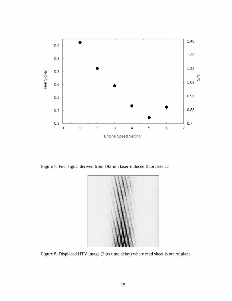
The 193-nm laser-induced fluorescence signal from the fuel is determined from the

undisplaced images and is depicted in Figure 7. The fuel signal is determined by using

the information obtained from the signal values less the value of the background value.

The fuel signal is in terms of an arbitrary pixel intensity. The fuel signal value provides

the best indicator of the fuel fluorescence. The fuel signal decreases with increasing

throttle setting due to less unburnt fuel being present in the flow as the throttle setting

increases.

Figure 6. SNR definition. (From a vertical line out at x=21.8 mm) To moderate the

influence of outliers (such as faulty pixels), N is estimated by 6 standard deviations, an

interval which contains about 99% of normally distributed noise.

15

Figure 7. Fuel signal derived from 193-nm laser-induced fluorescence

Figure 8. Displaced HTV image (3 µs time delay) where read sheet is out of plane

0.7

0.83

0.96

1.09

1.22

1.35

1.48

8000 10000 12000 14000 16000

0.3

0.4

0.5

0.6

0.7

0.8

0.9

0 1 2 3 4 5 6 7

S/N

Fuel S

ignal

Engine Speed Setting

16

Table 2. Image pairs and intersection

Engine

Setting

No. Image

Pairs

Grid

Intersections

Specified

No. Possible

Intersections

No. Actual

Intersections

Located

1 20 38 760 364

2 20 33 660 364

3 20 38 760 259

4 20 33 660 203

5 20 32 640 154

6 20 37 740 310

Table 2 represents the number of image pairs, number of intersections per image,

possible resulting intersections, and the actual intersections found. A total of 50 image

pairs were obtained for each throttle setting. Due to optical vibration, the read sheet

moved out of the plane of interest in some images (Figure 8); thus they were not usable.

For each condition, the 20 best images were chosen for analysis. The number of usable

intersections is dependent on the ability of the software to correlate the intersections in

the source and roam windows with a sufficiently high correlation coefficient value. The

low number of actual intersections located by the software can be attributed to the low

values of signal-to-noise in the images.

Figure 9 illustrates the velocity vectors obtained from averaging the HTV data at

each point for engine setting 3. In this depiction, the average velocity is 177 m/s for the

centerline flow of the engine exhaust at the nozzle exit. The velocity vectors from Figure

9 are superimposed on an undisplaced image in Figure 10. Figure 10b, a small region

denoted in Figure 10a is expanded to see the velocity vectors better. Most of the

displacement errors are in the y direction due to the elongated nature of the cross-sections

formed at 24º. For the 24º crossings, the spatial correlation program can determine the

horizontal displacement about 10 times more accurately than the vertical direction

(Gendrich 1999).

17

Figure 9. HTV derived centerline velocity vectors for engine setting 3 at the nozzle exit.

Figure 10. HTV derived centerline velocity vectors for engine setting 3 superimposed on

an undisplaced image (a) velocity magnitude and (b) expanded view of velocity

magnitude

18

2.4.1 Uncertainty

The uncertainty in the velocity data depends on two factors: uncertainty in timing

between the write-read lasers, Δt, and the uncertainty in measuring the displacement, d,

as follows:

dtdv

d

212

t

2

dv

(3)

where σi is the rms deviation of the ith quantity, v is the velocity, d is the displacement

and Δt is the time delay. The timing uncertainty between the firing of the two lasers is

±5 ns due to electronics jitter over the time delay of 3-9 µs. Thus the timing uncertainty

is less than 0.2% and can be neglected compared to the displacement error. Based on the

calculations of Gendrich and Koochesfahani (1999), the uncertainty in determining the

displacement for images of SNR 2 would be about 0.5 pixels for a displacement

measurement in the x (centerline) direction shown in Figure 9. So for the average

displacement of 9.82 pixels, this would result in 5% accuracy.

Figure 11. Measured velocity derived from HTV data.

0

100

200

300

400

500

600

0 1 2 3 4 5 6 7

Measure

d V

elo

city,

m/s

Engine Speed Setting

19

2.5 Dual-pulse and single image method comparison

The measured average and rms deviation of the velocity versus engine speed for

the dual-pulse method are displayed in Figure 11. The error bars indicate the rms

deviation velocities. The measured average velocity is velocity in the x (centerline)

direction. At the idle condition a velocity magnitude of 76 m/s is measured and the

velocity ramps up to a value of 580 m/s at full throttle.

This study provided a means for comparing the previous single-image method to

the current dual-pulse method. The single image method, utilized by Blandford et al.

(2008), was executed by marking both the undisplaced (0 µs) and displaced image with

OH fluorescence. With this method, one undisplaced image is taken prior to the engine

test and is used with each displaced image. Alternatively, the dual-pulse method employs

the use of image pairs taken in quick succession to determine velocity. To simulate the

single-image method, one undisplaced image from the group of image pairs was chosen

and used for analysis with each delayed image. The resulting comparison is portrayed in

Figure 12. Displayed are the velocity rms deviations from the mean in percent. From

this comparison, it can be seen that using the dual-pulse method results in a lower rms

deviation from the mean. This is attributed to reducing the effect of engine vibration.

There is about a 20% reduction in rms velocity deviation with respect to the mean

velocity across the entire range. The largest reductions in the absolute value of the rms

are at engine setting 1 and engine setting 4 where the grid displacement is the smallest

(~0.7 mm from Table 1); for example, at engine setting 4 the rms is reduced from 13% to

9.7% by using the dual-pulse method. The most accurate HTV measurement is at full

20

throttle (engine setting 6) where the displacement is the longest at ~1.8 mm and the

measurement uncertainty is about 4% for the dual-pulse method.

The major error in the velocity measurement is in the determination of the grid

displacement for the low signal grids. If most of the rms velocity deviation is due to error

in measurement of the grid displacement, the rms velocity should follow Equation (3)

. Figure 13 gives the rms velocity deviations versus the reciprocal of the

pixel displacements given in Table 1. From the rms velocity percent deviation, a pixel

displacement error can be estimated. Two trend lines with slopes of 0.45 and 0.55 (for

the dual-pulse and single-image methods, respectively are plotted. As can be seen, the

points for each throttle setting lie closely to these lines, indicating that the average

uncertainty in determining the displacement is ±0.55 pixels for the single-image method

and ±0.45 pixels for the dual-pulse method. The elimination of vibration effects leads to

a reduction of error from 0.55 to 0.45 pixels, which is a 20% relative decrease. Since

errors add like the sum of squares [i.e., see Equation (3)], the vibration error corresponds

to an rms value of 0.3 pixels (~50 microns). It appears that the rms velocity in the

measurement in mostly a result of the displacement measurement error due to the low

signal-to-noise of the HTV images.

21

Figure 12. Comparison of dual-pulse and single-image method velocity deviation from

the mean for J-85 jet engine.

Figure 13. Velocity uncertainty from the mean derived from HTV data, where dx is the

average centerline displacement from Table 1.

2

4

6

8

10

12

14

2

4

6

8

10

12

14

0 1 2 3 4 5 6 7

RM

S D

evia

tion %

Engine Speed Setting

Single Image Method

Dual Pulse Method

3 µs delay

9 µs delay

0

2

4

6

8

10

12

14

16

0 0.05 0.1 0.15 0.2 0.25

Ve

locity U

nce

rta

inty

, σ

v/v

(%)

1/dx

Dual-Pulse Method

Single-Image Method

0.45 pixels

0.55 pixels

3

5

2

4 1

6

22

2.6 Conclusion

The HTV method has been improved using a dual-pulse method that reduces the

deleterious effects of vibration on the HTV measurement accuracy. The dual-pulse

method is applied to a J85 jet engine exhaust to measure centerline velocities from 76 m/s

at the lowest speed setting ramping up to 580 m/s at the highest speed setting. Using

spatial correlation software, the velocities are measured from HTV images in spite of the

low quality of the images. By using the dual-pulse feature of the intensified CCD

camera, the measurement uncertainty was lowered about 20% (e.g. rms velocity deviation

at full throttle decreased from 5% to 4%) when the vibration effect on displacement error

was eliminated. The measured rms velocity deviations ranged from 4% to 14% and most

of the rms velocity deviation is attributed to the measurement error in determining the

displacement of the low signal images. Shorter grid displacements led to lower accuracy.

Computer software developed by Gendrich and Koochesfahani (1999) determined the

displacement in the images to about ±0.5 pixels. By analyzing the images with a single-

image method and dual-pulse method, the rms value of the displacement was found to

decrease from 0.55 to 0.45 pixels; this leads to an estimate of 0.3 pixels (~50 µm) rms

deviation due to vibration when using the single-image method. Engine vibration also

caused out of plane movement of the OH read sheet that led to displaced grid images that

was not usable. With the 11x11 grid, multiple velocity vectors were obtained from a

single image. By using the dual-pulse method in conjunction with the processing

program, future studies can be done to efficiently determine velocities of other flows and

devices.

23

CHAPTER III

Investigation of a Bow Shock Using HTV

3.1 Introduction

Molecular tagging velocimetry (MTV) is commonly used to characterize fluid

flows (Wehrmeyer 1999; Pitz 2000; Lahr 2010; Barker 1998). MTV has been employed

by several researchers to determine temperature and velocity in flows to characterize

shock waves. Many of these methods include the use of Planar Laser-Induced

Fluorescence (PLIF) to investigate oblique and bow shocks formed in cavities and around

blunt and sharp-edged objects to simulate hypersonic flow for aerospace applications

(Jeong 2008; Houwing 2001; Smith 1994; Ruyten 1998; Danehy 2001, 2003; Davidson

1991).

Previously, Smith et al. (1994) applied PLIF of NO to a shock tube flow with Ms

of 2.0 and 2.5 for two conical test articles, one with a sharp tip and one blunt-nosed. The

PLIF measurements were conducted as a preliminary means for demonstration,

validation, and calibration of facility diagnostic systems such as planar temperature

measurement. The experiment produced temperatures between 1000 and 1500 K. To

further explore the shock tube flow, the present study employs HTV to determine the

velocity downstream of the initial shock wave. The shock tube features pressure

transducers which are used to determine shock speed. The HTV images are analyzed

using a new template matching correlation technique (Ramsey 2011) to determine

displacements of the grid intersections and thereby the two-dimensional velocity

distribution downstream of the initial shock wave.

24

3.2 Experimental System

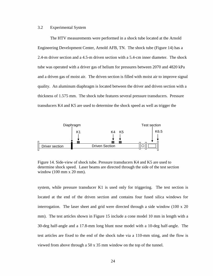
The HTV measurements were performed in a shock tube located at the Arnold

Engineering Development Center, Arnold AFB, TN. The shock tube (Figure 14) has a

2.4-m driver section and a 4.5-m driven section with a 5.4-cm inner diameter. The shock

tube was operated with a driver gas of helium for pressures between 2070 and 4820 kPa

and a driven gas of moist air. The driven section is filled with moist air to improve signal

quality. An aluminum diaphragm is located between the driver and driven section with a

thickness of 1.575 mm. The shock tube features several pressure transducers. Pressure

transducers K4 and K5 are used to determine the shock speed as well as trigger the

Figure 14. Side-view of shock tube. Pressure transducers K4 and K5 are used to

determine shock speed. Laser beams are directed through the side of the test section

window (100 mm x 20 mm).

system, while pressure transducer K1 is used only for triggering. The test section is

located at the end of the driven section and contains four fused silica windows for

interrogation. The laser sheet and grid were directed through a side window (100 x 20

mm). The test articles shown in Figure 15 include a cone model 10 mm in length with a

30-deg half-angle and a 17.8-mm long blunt nose model with a 10-deg half-angle. The

test articles are fixed to the end of the shock tube via a 110-mm sting, and the flow is

viewed from above through a 50 x 35 mm window on the top of the tunnel.

Test section

Driver section Driven Section

K4 K5 K1 K6.5

Diaphragm

25

Figure 15. Test articles for experiment. Cone model (top) and blunt nose model

(bottom). Each test article is attached to a 110 mm sting.

To interrogate the flow, a tunable 193-nm ArF excimer laser (Lambda Physik

COMPex 150-T, 193-194 nm) with output energy of 150 mJ per pulse, 0.2 mrad

divergence, and a pulse duration of 20 ns was used to photodissociate the water vapor to

produce OH radicals. The ArF laser was operated in broadband mode at 193.4 nm (0.5

nm bandwidth). The ArF beam, 20 mm high by 10 mm wide, was split via a beam

splitter. The split beam was sent into grid forming optics. The grid forming optics

consist of two sets of optics closely spaced: a 300-mm focal length cylindrical lens (25 x

40 mm) and a stack of 11 cylindrical lenses (20 mm long x 2 mm wide). Each set of grid

optics forms 11 parallel beams with exit energy of ~14mJ (~1.0 mJ/beam). The two sets

of 11 beams are crossed at a 34 deg angle. The OH radicals were excited via an Nd:YAG

(Continuum Lasers Powerlite 9010) pumped tunable dye laser with an ultraviolet

wavelength extender. The doubled output of the dye laser is tuned to excite the strong

Q1(1) line in the A2

+( v =1)←X

2i( v =0) OH band at a wavelength of 281.997 nm

(35461.330 cm-1

). The dye laser wavelength and the Q1(1) line position were determined

by fluorescence excitation spectra taken in room air, as done previously (Blandford 2008;

Alexander 2008). The ~282-nm beam (~8 mJ/pulse) was expanded by a negative

26

cylindrical lens (focal length -125 mm) and focused into a sheet 27 mm wide by 0.3

mm thick with a 500-mm focal length spherical lens.

The images were recorded using an intensified interline CCD camera (Princeton

Instruments PI-MAX II 1024x1024 pixels). The fluorescence light was collected by a

105-mm focal length f/4.5 UV Nikon camera lens positioned 244 mm above the test

section. To capture the OH fluorescence near ~305-325 nm and block interfering

background light from the lasers (193-nm, 282-nm), a Schott UG-ll (1 nm thick) filter

and a WG305 (3 mm thick) filter were used in front of the camera lens to create a

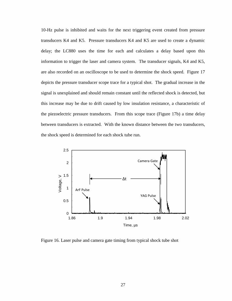
bandpass filter from 305 to 375 nm. Figure 16 shows the laser pulse and camera gate

timing from a typical shock tube run. The ArF laser pulse and Nd:YAG pulse are

separated by a time of Δt=1 µs that sets the time of flight. The camera gate captures the

delayed image after the shock has travelled past the test article but before the reflected

shock travels back past the test article. The average undelayed image was generated by

recording 100 grid images in room air before testing began at atmospheric pressure and

averaging them. The camera image was calibrated by placing a ruler in the focal plane

giving a factor of 34.71±0.25 pix/mm that is used to determine velocities. Thus, the laser

line is about 11 pixels in diameter. The 1024 x 1024 pixel images correspond to a 29.5 x

29.5 mm area in the shock tube.

The synchronization of the laser and camera were controlled via a programmable

experiment controller (LabSmith LC880) with ~17 ns jitter. Before the firing of the

tunnel, the Nd:YAG laser is run at 10 Hz to ensure that it is at proper “warming

conditions.” Once the shock tube gasses are filled, a valve is opened and the shock

begins its path. Once the shock passes pressure transducer K1 (Figure 14), the Nd:YAG

27

10-Hz pulse is inhibited and waits for the next triggering event created from pressure

transducers K4 and K5. Pressure transducers K4 and K5 are used to create a dynamic

delay; the LC880 uses the time for each and calculates a delay based upon this

information to trigger the laser and camera system. The transducer signals, K4 and K5,

are also recorded on an oscilloscope to be used to determine the shock speed. Figure 17

depicts the pressure transducer scope trace for a typical shot. The gradual increase in the

signal is unexplained and should remain constant until the reflected shock is detected, but

this increase may be due to drift caused by low insulation resistance, a characteristic of

the piezoelectric pressure transducers. From this scope trace (Figure 17b) a time delay

between transducers is extracted. With the known distance between the two transducers,

the shock speed is determined for each shock tube run.

Figure 16. Laser pulse and camera gate timing from typical shock tube shot

0

0.5

1

1.5

2

2.5

1.86 1.9 1.94 1.98 2.02

Voltage,

V

Time, µs

ArF Pulse

Camera Gate

YAG Pulse

Δt

28

Figure 17. Pressure transducer scope traces (a) K4 scope trace to indicate incident and

reflected shock location (b) K4 and K5 scope trace. K4 and K5 are used to determine

incident shock speed.

0

1

2

3

4

5

6

7

-4 -3 -2 -1 0 1 2 3 4

Voltage,

V

Time, ms

incident shock

reflected shock

0

1

2

3

4

5

6

7

-4 -3 -2 -1 0 1 2 3 4

Voltage,

V

Time, ms

K4

K5

incident shock

reflected shock

(a)

(b)

29

To demonstrate the repeatability of the shock tube, the measured and calculated shock

speeds are determined for comparison (Figure 18). The measured shock speed is

determined from the aforementioned measurement via K4 and K5, while the calculated

shock speed is determined from shock theory equation,

112

1

1

2

1

11

P

PaWs

(4)

where the properties of air are assumed and the pressure ratio is determined from

the initial driven and driver pressures, given by:

12

12111

12414

1

2

1

4

44

1122

111

PP

PPaa

P

P

P

P (5)

The pressure transducers do a relatively good job of determining shock speed. The

outliers in Figure 18 are unexplained and may be due to non-ideal shock tube

performance from a diaphragm that did not completely open.

Figure 18. Measured and calculated shock speed comparison

800

1000

1200

1400

1600

1800

800 1000 1200 1400 1600 1800

Ws m

easure

d, m

/s

Ws calculated, m/s

Data

Expected

30

3.3 Experimental Results

The experiment was conducted for three test conditions for each test article.

Table 3 gives the measured time between pressure transducers K4 and K5, the measured

and calculated shock speeds, and the pressure ratio derived from the measured shock

speed. The calculated shock speed was derived from shock theory using the known

driven and driver pressures. The pressure ratio was determined from the following 1D

shock equation,

111

22

11

1

1

2

a

W

P

P s

(6)

assuming the properties of air. From this it can be inferred that pressure transducers K4

and K5 can measure the shock speed within 10% of what theory predicts if the extreme

outliers in Figure 18 are ignored.

Table 3. Measured and calculated shock speed. The calculated shock speed is

determined from P4/P1 using Equation 4 and 5. The pressure ratio P2/P1 is calculated

from the measured shock speed using Equation 6. * Pressure, P4 ,for test condition 6

could not be accurately determined.

Measured

ΔtK4-K5, µs

Measured

Ws, m/s

P2/P1 P4/P1 Calculated

Ws, m/s

Blunt Nose Model

1 228 1340 17.4 113 1280

2 200 1530 22.7 243 1480

3 188 1620 25.7 425 1630

Cone Model

4 216 1410 19.5 108 1270

5 208 1470 21.0 204 1440

6 214 1660 26.9 * *

31

The HTV images were analyzed using a template matching method developed by

Ramsey and Pitz (2011) to determine the displacements of the grid intersections. This

automated code locates the grid intersections in each image by optimizing the correlation

with a simulated surface (or template) defined by the sum of two Gaussian prisms

corresponding to the two laser lines. The simulated surface has six degrees of freedom

which are optimized for each intersection, including two location coordinates, the angle

of each line, the Gaussian width of the two lines (assumed equal), and the relative

intensity of the two lines. After all intersections are fit, corresponding intersection

parameters in each undisplaced/displaced image pair are compared, and both linear and

angular displacements can be determined. Dividing these by the known delay time t

yields 2D velocity and two of its directional derivatives, along with information on signal

and noise levels. In the current study, the angular degrees of freedom were not utilized

since there is very little angular movement in the grid. When compared to the direct

spatial correlation method employed by Gendrich and Koochesfahani

(1999), the

template method has improved results for the low resolution images typically used in

HTV (Ramsey 2011).

The recorded HTV images are used to determine the gas velocity downstream of the

shock wave, up. This experimental value is compared to theoretical value of up calculated

from the pressure ratio determined from the measured shock speed according to the 1D

shock relation:

1

1

1

2

1

1

1

1

2

1

1

1

2

1

1

P

PP

Pau p (7)

32

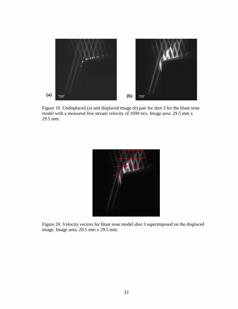
3.3.1 Blunt Nose Model

Figure 19 shows the undisplaced image and displaced image for shot 3 for the blunt

nose model. The grid is positioned such that both the velocity in front and behind the

shock can be visualized. The undisplaced image (Figure 19a) is imaged in room air at

standard temperature and pressure before the experiment is begun; this method is used

since vibration is not of major concern. The bright dots are where the laser beams hit the

model surface. The displaced image (Figure 19b) shows the defined shock front as the

shock passes the test article as the HTV grid is much brighter in the region behind the

shock. By using the time delay of 1±0.05 µs between the firing of the lasers and the

displacement between the undisplaced and displaced image, an average freestream

velocity of up=1690 m/sec is determined. Also from this image one can infer in the

postshock region that there is a temperature increase indicated by an increase in OH LIF

signal behind the shock.

The velocity vectors that result from determining displacements in Figure 19 are

shown in Figure 20 along with the shock front. The vectors indicate that the velocity is

largest ahead of the shock front and then slows behind the shock. This result is also

shown in Figure 21, with a minimum average value of 1250 m/sec behind the shock.

33

Figure 19. Undisplaced (a) and displaced image (b) pair for shot 3 for the blunt nose

model with a measured free stream velocity of 1690 m/s. Image area: 29.5 mm x

29.5 mm.

Figure 20. Velocity vectors for blunt nose model shot 3 superimposed on the displaced

image. Image area: 29.5 mm x 29.5 mm.

(a) (b)

34

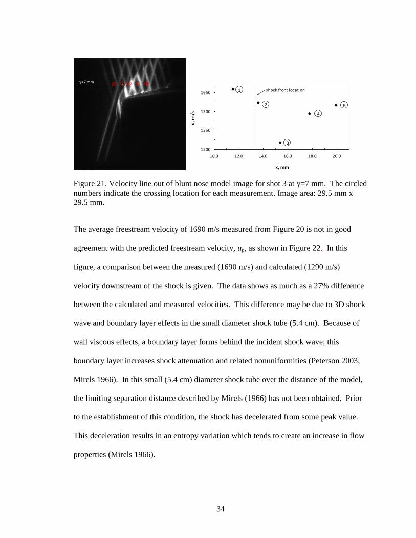
Figure 21. Velocity line out of blunt nose model image for shot 3 at y=7 mm. The circled

numbers indicate the crossing location for each measurement. Image area: 29.5 mm x

29.5 mm.

The average freestream velocity of 1690 m/s measured from Figure 20 is not in good

agreement with the predicted freestream velocity, up, as shown in Figure 22. In this

figure, a comparison between the measured (1690 m/s) and calculated (1290 m/s)

velocity downstream of the shock is given. The data shows as much as a 27% difference

between the calculated and measured velocities. This difference may be due to 3D shock

wave and boundary layer effects in the small diameter shock tube (5.4 cm). Because of

wall viscous effects, a boundary layer forms behind the incident shock wave; this

boundary layer increases shock attenuation and related nonuniformities (Peterson 2003;

Mirels 1966). In this small (5.4 cm) diameter shock tube over the distance of the model,

the limiting separation distance described by Mirels (1966) has not been obtained. Prior

to the establishment of this condition, the shock has decelerated from some peak value.

This deceleration results in an entropy variation which tends to create an increase in flow

properties (Mirels 1966).

y=7 mm1 2 3 4 5

y=7 mmy=7 mm1 2 3 4 51 2 3 4 5

1200

1350

1500

1650

10.0 12.0 14.0 16.0 18.0 20.0

x, mm

u, m

/s

shock front location1

5

4

3

2

35

To complete the analysis of the blunt nose model, the stand-off distance Δd at the

stagnation point of the blunt nose model for the three shock tube shots is displayed

(Figure 23). From this plot it is confirmed that as the Mach number is decreased, the

stand-off distance is increased, indicating a shock that is becoming increasingly detached

as shown by Satheesh et al. (2007).

Figure 22. Measured and calculated velocity downstream of shock for blunt nose model.

Figure 23. Standoff distance, Δd, from the stagnation point of the blunt nose model for

the three shock tube shots.

1000

1200

1400

1600

1800

1000 1200 1400 1600 1800

up, m

easure

d, m

/s

up calculated, m/s

Data

Expected

1.0

1.1

1.2

1.4

1.5

1.6

1.6 1.7 1.8 1.9 2.0 2.1 2.2

Δd, m

m

up/a2

Δd

36

3.3.2 Cone Model

The experiment was also conducted on a 30 degree half-angle cone model

(Figure 15). The cone model’s undisplaced and displaced images are displayed in

Figure 24. Again, the average undisplaced image is obtained before the experiment is

begun and is used to determine displacement. With the given time delay and

displacement, an average freestream velocity of 1610 m/sec is calculated which compares

to 1320 m/s from Equation 7. The resulting velocity vectors are displayed in Figure 25

along with the shock front. The velocity ahead of the shock has the highest speed and

slows past the shock. The velocity behind the shock not only slows, but also contours

away from the cone model. As with the blunt nose model, the measured and calculated

freestream velocities produced by the incident shock wave do not closely lie with theory.

However, for the cone model data set, HTV measurements of freestream velocity are

closer to those predicted by Equation 7 as seen in Figure 26. Since this model has a sharp

edge, versus the blunt edge of the previous model, the shock is attached and a shock

angle can be determined. In Figure 27 the wave angle is plotted versus the measured

shock speed, where the calculated wave angle is determined using the shock speed and

shock properties curve, Chart 5, from NACA Report 1135 (1953). According to the

theoretical calculations and as indicated by the calculated data set, the wave angle should

decrease with increasing shock speed. As shown, there is a 14% difference between the

measured and calculated values of the wave angle, except in the first data point. This

difference is consistent with a higher freestream velocities found in the measurement.

This data point may be attributed to random disturbances caused by the shock tube firing

37

that may have displaced the model away from the shocktube centerline to result in an

incorrect angle measurement.

Figure 24. Undisplaced and displaced image pair for shot 6 for the cone model with a

measured shock speed of 1660 m/s. Image area: 29.5 mm x 29.5 mm.

Figure 25. Velocity vectors for cone model shot 6 superimposed on the displaced image.

Image area: 29.5 mm x 29.5 mm.

(a) (b)

38

Figure 26. Measured and calculated velocity downstream of shock for the cone model

Figure 27. Measured and calculated wave angle for the cone model

1000

1200

1400

1600

1800

1000 1200 1400 1600 1800

up m

easure

d, m

/s

up calculated, m/s

Data

Expected

44.0

48.0

52.0

56.0

60.0

1400 1500 1600 1700

Wave a

ngle

,degre

es

Ws, m/s

βmeasured

βcalculated

39

3.4 Conclusion

HTV has been demonstrated in a high-speed flow using a grid that provides 2D

velocity data. The use of the 11 x 11 grid allows for multiple velocity vectors to be

obtained from a single image. The method was applied to two test articles, a blunt nose

model and a cone model, to determine the velocity of the gas downstream of the shock

wave. Measurements of the induced velocity, up, of the gas downstream of the incident

shock are as high as 1690 m/sec but vary from the theoretical values by as much as 27%.

By utilizing the installed pressure transducers along the shock tube, the shock speed can

be determined within 10% of theoretical values, validating their use to derive the pressure

ratio and other calculated quantities. Although the measured shock speeds reliably align

with the theory, the induced velocity downstream of the shock does not. This can be

attributed to the 1D shock theory used not taking into account 3D effects or boundary-

layer growth in the small diameter shock tube (5.4 cm). By implementing more complex

theoretical analysis, accounting for the 3D body, the aforementioned measurements can

provide a means for validating theoretical codes and CFD.

40

REFERENCES

Alexander, A., J. Wehrmeyer, W. Runge, B. Blandford, A.V. Anilkumar and R. Pitz

(2008). “Nonintrusive measurement of gas turbine exhaust velocity using

hydroxyl tagging velocimetry,” 26th

AIAA Aerodynamic Measurement

Technology and Ground Testing Conf., Paper No. AIAA-2008-3209, Seattle,

WA.

Barker, P.F., A.M. Thomas, T.J. McIntyre and H. Rubinsztein-Dunloop (1998).

“Velocimetry and thermometry of supersonic flow around a cylindrical body,”

AIAA Journal 36: 1055-1060.

Blandford, B.T., W.O. Runge, S. Hu, A.V. Anilkumar, R.W. Pitz and J. A. Wehrmeyer

(2008). “Application of hydroxyl tagging velocimetry (HTV) to measure

centerline velocities in the near field exhaust of a gas turbine engine,” 46th

AIAA

Aerospace Sciences Meeting, Reno, Paper No. AIAA-2008-0235, Reno, NV.

Danehy, P.M., P. Mere, M.J. Gaston, S. O’Byrne, P.C. Palma and A.F.P. Houwing

(2001). “Fluorescence velocimetry of the hypersonic, separated flow over a

cone,” AIAA Journal 39: 1320-1328.

Danehy, P.M., S. O’Byrne, A.F.P. Houwing, J.S. Fox and D.R. Smith (2003). “Flow-

tagging velocimetry for hypersonic flows using fluorescence of nitric oxide,”

AIAA Journal 41: 263-271.

Davidson, D.F., A.Y. Chang, M.D. DiRosa and R.K. Hanson (1991). “Continuous wave

laser absorption techniques for gas dynamic measurements in supersonic flows,”

Applied Optics 30: 2598-2608.

Fajardo, C. and V. Sick (2009). “Development of high-speed UV particle image

velocimetry technique and application for measurements in internal combustion

engines,” Experiments in Fluids 46: 43-53.

Gendrich, C.P. and M.M. Koochesfahani (1999). “A spatial correlation technique for

estimating velocity fields using molecular tagging velocimetry (MTV),”

Experiments in Fluids 22: 67-77.

Gere, J.M. and S.P. Timoshenko (1997). “Mechanics of Materials,” 4th

Edition, Boston:

PWS Publishing Company.

Houwing, A.F.P., D.R. Smith, J.S. Fox, P.M. Danehy and N.R. Mudford (2001).

“Laminar boundary layer separation at a fin-body junction in a hypersonic flow,”

Shock Waves 11: 31-42.

41

Hsu, A.G., R. Srinivasan, R.D.W. Bowersox, S.W. North (2009). “Molecular tagging

using vibrationally excited nitric oxide in an underexpanded jet flowfield,” AIAA

Journal 47: 2597-2604.

Ismailov, M.M, H.J. Schock and A.M. Fedewa (2006). “Gaseous flow measurements in

an internal combustion engine assembly using molecular tagging velocimetry,”

Experiments in Fluids 41: 57-65.

Jeong, E., S. O’Byrne, I.S. Jeung and A.F.P. Houwing (2008). “Investigation of

supersonic combustion with angled injection in a cavity-based combustor,”

Journal of Propulsion and Power 24: 1258-1268.

Lahr, M.D., R.W. Pitz, Z.W. Douglas and C.D. Carter (2010). Hydroxyl tagging

velocimetry measurements of a supersonic flow over a cavity,” Journal of

Propulsion and Power 26: 790-797.

Lee, M.P. and R.K. Hanson (1986). “Calculations of O2 absorption and fluorescence at

elevated temperatures for a broadband argon-fluoride laser source at 193 nm,”

Journal of Quantitative Spectroscopy and Radiative Transfer 36: 425-440.

Miles, R.B., J. Grinstead, R.H. Kohl and G. Diskin (2000). “The RELIEF flow tagging

technique and its application in engine testing facilities and for helium-air mixing

studies,” Measurement Science and Technology 11: 1272-1281.

Mirels, H. (1966). “Flow nonuniformity in shock tubes operating maximum test times,”

The Physics of Fluids 9: 1907-1912.

Mittal, M., R. Sadr, H.J. Schock, A. Fedewa and A. Naqwi (2009). “In-cylinder engine

flow measurement using stereoscopic molecular tagging velocimetry (SMTV),”

Experiments in Fluids 46: 277-284.

NACA (1953). Report 1135 Equations, Tables, and Charts for Compressible Flow.

Report 1135, Ames Aeronautical Laboratory, Moffett Field, CA.

Peterson, E.L. and R.K. Hanson (2003). “Improved turbulent boundary-layer model for

shock tubes,” AIAA Journal 41: 1314-1322.

Pitz, R.W., J.A. Wehrmeyer, L.A. Ribarov, D.A. Oguss, F. Batliwala, P.A. DeBarber, S.

Deusch and P.E. Dimotakis (2000). “Unseeded molecular flow tagging in cold

and hot flows using ozone and hydroxyl tagging velocimetry,” Measurement

Science and Technology 11: 1259-1271.

Pitz, R.W., M.D. Lahr, Z.W. Douglas, J.A. Wehrmeyer, S. Hu, C.D. Carter, K.Y. Hsu, C.

Lum and M.M. Koochesfahani (2005). “Hydroxyl tagging velocimetry in a

supersonic flow over a cavity,” Applied Optics 44: 6692-6700.

42

Ramsey, M.C. and R.W. Pitz (2011). “Template matching for improved accuracy in

molecular tagging velocimetry,” Experiments in Fluids 51: 811-819.

Ribarov, L.A., J.A. Wehrmeyer, R.W. Pitz and R.A. Yetter (2002). “Hydroxyl tagging

velocimetry (HTV) in experimental airflows,” Applied Physics B 74: 175-183.

Ribarov, L.A., S. Hu, J.A. Wehrmeyer and R.W. Pitz (2005). “Hydroxyl tagging

velocimetry method optimization: signal intensity and spectroscopy,” Applied

Optics 44: 6616-6626.

Ruyten, W.M., M.S. Smith, L.L. Price and W.D. Williams (1998). “Three-line

fluorescence thermometry of optically thick shock-tunnel flow,” Applied Optics

37: 2334-2339.

Satheesh, K., G. Jagadeesh and K.P.J. Reddy (2007). “High speed schlieren facility for

visualization of flow fields in hypersonic shock tunnels,” Current Science 92: 56-

60.

Sijtsema, N.M., N.J. Dam, J.H. Klein-Douwel and J.J. ter Meulen (2002). “Air photolysis

and recombination tracking: a new molecular tagging velocimetry scheme,”

AIAA Journal 40: 1061-1064.

Smith, M.S., W.D. Williams, L.L. Price and J.H. Jones (1994). “Shocktube planar laser

induced fluorescence measurements in support of the AEDC impulse facility,”

18th

AIAA Aerospace Ground Testing Conference, Paper No. AIAA-94-2649,

Colorado Springs, CO.

Stier, B. and M.M. Koochesfahani (1999). “Molecular tagging velocimetry (MTV)

measurements in gas phase flows,” Experiments in Fluids 26: 297-304.

Timmerman, B.H., A.J. Skeen, P.J. Bryanston-Cross and M.J. Graves (2009). “Large-

scale time-resolved digital particle image velocimetry (TR-DPIV) for

measurement of high subsonic hot coaxial jet exhaust of a gas turbine engine,”

Measurement Science and Technology 20: 074002 (15pp) DOI 10.108810957-

0233/20171074002.

Wehrmeyer, J.A., L.A. Ribarov, D.A. Oguss and R.W. Pitz (1999). “Flame flow tagging

velocimetry with 193-nm H2O photodissociation,” Applied Optics 38: 6912-6917.