NASA/TM-2002-211630

Flow Visualization of Density in a Cryogenic Wind Tunnel Using Planar Rayleigh and Raman Scattering

Gregory C. Herring and Behrooz ShirinzadehLangley Research Center, Hampton, Virginia

June 2002

The NASA STI Program Office . . . in Profile

Since its founding, NASA has been dedicated to the advancement of aeronautics and space science. The NASA Scientific and Technical Information (STI) Program Office plays a key part in helping NASA maintain this important role.

The NASA STI Program Office is operated by Langley Research Center, the lead center for NASA

’

s scientific and technical information. The NASA STI Program Office provides access to the NASA STI Database, the largest collection of aeronautical and space science STI in the world. The Program Office is also NASA

’

s institutional mechanism for disseminating the results of its research and development activities. These results are published by NASA in the NASA STI Report Series, which includes the following report types:

•

TECHNICAL PUBLICATION. Reports of completed research or a major significant phase of research that present the results of NASA programs and include extensive data or theoretical analysis. Includes compilations of significant scientific and technical data and information deemed to be of continuing reference value. NASA counterpart of peer-reviewed formal professional papers, but having less stringent limitations on manuscript length and extent of graphic presentations.

•

TECHNICAL MEMORANDUM. Scientific and technical findings that are preliminary or of specialized interest, e.g., quick release reports, working papers, and bibliographies that contain minimal annotation. Does not contain extensive analysis.

•

CONTRACTOR REPORT. Scientific and technical findings by NASA-sponsored contractors and grantees.

•

CONFERENCE PUBLICATION. Collected papers from scientific and technical conferences, symposia, seminars, or other meetings sponsored or co-sponsored by NASA.

•

SPECIAL PUBLICATION. Scientific, technical, or historical information from NASA programs, projects, and missions, often concerned with subjects having substantial public interest.

TECHNICAL TRANSLATION. English-language translations of foreign scientific and technical material pertinent to NASA

’

s mission.

Specialized services that complement the STI Program Office

’

s diverse offerings include creating custom thesauri, building customized databases, organizing and publishing research results . . . even providing videos.

For more information about the NASA STI Program Office, see the following:

•

Access the NASA STI Program Home Page at

http://www.sti.nasa.gov

•

Email your question via the Internet to help@sti.nasa.gov

•

Fax your question to the NASA STI Help Desk at (301) 621-0134

•

Telephone the NASA STI Help Desk at (301) 621-0390

•

Write to:NASA STI Help DeskNASA Center for AeroSpace Information7121 Standard DriveHanover, MD 21076-1320

National Aeronautics andSpace Administration

Langley Research CenterHampton, Virginia 23681-2199

NASA/TM-2002-211630

Flow Visualization of Density in a Cryogenic Wind Tunnel Using Planar Rayleigh and Raman Scattering

Gregory C. Herring and Behrooz ShirinzadehLangley Research Center, Hampton, Virginia

June 2002

Available from:

NASA Center for AeroSpace Information (CASI) National Technical Information Service (NTIS)7121 Standard Drive 5285 Port Royal RoadHanover, MD 21076-1320 Springfield, VA 22161-2171(301) 621-0390 (703) 605-6000

Acknowledgments

We thank W. E. Lipford and M. T. Fletcher for help with the installation of the laser setup, A. Seifert and L. G.Pack for helpful discussions, and M. Kulick for fabrication of the modified off-block.

The use of trademarks or names of manufacturers in this report is for accurate reporting and does not constitute anofficial endorsement, either expressed or implied, of such products or manufacturers by the National Aeronautics andSpace Administration.

Abstract

Using a pulsed Nd:YAG laser (532 nm) and a gated, intensifiedcharge-coupled device, planar Rayleigh and Raman scattering tech-niques have been used to visualize the unseeded Mach 0.2 flow density ina 0.3-meter transonic cryogenic wind tunnel. Detection limits are de-termined for density measurements by using both unseeded Rayleigh andRaman (N2 vibrational) methods. Seeding with CO2 improved theRayleigh flow visualization at temperatures below 150 K. The seededRayleigh version was used to demonstrate the observation of transientflow features in a separated boundary layer region, which was excitedwith an oscillatory jet. Finally, a significant degradation of the laserlight sheet, in this cryogenic facility, is discussed.

Introduction

NASA Langley Research Center (LaRC) has an ongoing effort (see citations in ref. 1) for the devel-opment of Rayleigh scattering (ref. 2) in a variety of wind tunnels. Many wind tunnels, including LaRC’s0.3-Meter Transonic Cryogenic Tunnel (TCT), operate near the condensation point of the working fluid;hence, clusters of molecules may form in the unseeded flow. With clusters, the quantitative aspect of thedensity measurement from the Rayleigh signal is compromised. Since the Rayleigh scatter is elastic andproportional to the sixth power of the cluster size, the scatter from the clusters can easily be larger thanthe molecular scatter. Since the cluster-size distribution is not typically known, the density of molecularscatters is hard to deconvolve from the cluster signal. In this case, Rayleigh scattering cannot easilymeasure flow density and is limited to qualitative flow visualization. Recently, (ref. 3) it was demon-strated that clustering does not occur in the free-stream flow for typical run conditions in the TCT, mak-ing Rayleigh scattering one promising method for quantitative density measurements in the TCT.

In this report, planar imaging of density in the unseeded flow is demonstrated in the TCT withRayleigh scattering from a laser beam formed into a sheet. Seeding CO2 into the flow is shown to induceclustering in the flow medium, increasing the magnitude of the elastic light scattering and enhancing thequality of the images. This seeded version of planar Rayleigh scattering is used to detect transient flowstructure downstream of the blowing slot in a near-zero-mass-flow oscillatory blowing experiment.Planar Raman scattering from the 0-1 vibrational transition in N2 is also demonstrated as a second poten-tial method to visualize the unseeded flow. Finally, beam steering effects, by the cryogenic fluid in TCT,are described.

The elastic light scatter is in the Rayleigh regime for the unseeded flow; however, adding CO2 toinduce clusters raises questions about the size of the clusters and whether the seeded elastic light scatter isin the Rayleigh or Mie regime. For the purpose of this work, it is not important if the elastic scatter is inthe Rayleigh or Mie regime, and we will hereafter refer to the seeded scattering as Rayleigh scattering.

Rayleigh and Raman Scattering

A summary of Rayleigh and Raman scattering is given in reference 4. The scattered light signal P(photoelectrons/sec) is given by

P = N(dσ/dΩ)90 L Pl ε η Ω (1)

2

The symbols are the solid angle Ω (sr) used to collect the signal, the transmission η of the collectionoptics from the sample volume to the detector cathode, the incident power Pl (photons/sec) of the laserbeam in the sample volume, the quantum efficiency ε of the detector cathode, the length L (m) of the laserbeam that is imaged on the detector, the differential scattering cross section per molecule (dσ/dΩ)90(m2/sr molecule) at 90° to the polarization direction and 90° to the beam propagation direction, and thenumber density N (molecules/m3) of the scattering medium.

Typically, the Rayleigh cross section is 103 times larger than the Raman cross section; hence,Rayleigh signals are large compared to Raman signals. However, because Rayleigh scattering is elastic,scattered laser light from windows and walls produces a background level that interferes with theRayleigh signal. Fluctuations in that background typically appear as the dominant noise on the Rayleighsignal. In contrast, the Raman signal is inelastic, shifted in energy by 2330 cm−1 in the case of the N2 0-1vibrational band that is used here. For laser excitation at 532 nm, a narrow-band interference filter, cen-tered at 607 nm, can be used to block the scattered light at the laser frequency. Thus, scattered light isminimal, and shot noise and dark current typically dominate the noise in the signal-to-noise ratio (SNR)of the Raman signal.

Experimental Setup

Wind Tunnel

This work was performed at the 0.3-m TCT at LaRC. It is a fan-driven, closed-circuit facility (ref. 5)designed to achieve large Reynolds numbers (~3 × 108/m) by using high-pressure (~5 × 105 MPa) andlow-temperature (~100 K) N2 as the flow medium. This two-dimensional tunnel has a test section widthof 33 cm and is used primarily for the testing of airfoil configurations.

The model consists of a 2.6-cm hump that is mounted on the sidewall. This configuration simulatesthe 2-dimensional flow over the upper surface of an airfoil. The hump model is described further in ref-erence 6. The oscillatory excitation experiment of reference 6 was designed to study the delay of flowseparation from a simulated airfoil at Mach 0.2 in a high Reynolds number flow. A sketch of the humpmodel and laser light sheet is shown in figure 1. The slot S2 is for oscillatory excitation of the flowfield.Near-room-temperature N2 was used as the driving fluid. There is typically a slight bias on the oscillatoryflow through slot S2 in favor of a small mass flow into the tunnel. This net mass flow into the tunnel issmall relative to the mass flow of the free-stream of the test section. In this study, after demonstratingthat we could visualize the unseeded flow, gaseous CO2 was seeded into the relatively warm N2 fluid thatis injected into the cold flow through the slot S2. The CO2 induces clustering and greatly increases thestrength of the scattered Rayleigh light.

For typical operation, the facility is cooled significantly below room temperature and will move 3 cmrelative to the concrete floor. Thus the laser, camera, and all optics are mounted directly on the tunnel tomaintain their position relative to the model during this thermal contraction. Upon cooling and pressur-izing, it was necessary to repeatedly enter the test cell and adjust the optical alignment. Since the outerwindow W2 is cold, it is necessary to purge the window surface with dry N2 to avoid the water condensa-tion. Since the Rayleigh and Raman scattered light is relatively small, it is important to have a good-quality purge since the slightest amount of condensation can degrade the Rayleigh images. The laser-beam path outside the tunnel should be shielded from the fog generated from the low-temperature air inthe test cell.

3

Optical Arrangement

The facility/model geometry and the limited optical access determined the observation region. Theoptical and electronic setup is similar to one used previously (ref. 7), with the exception that the excimerlaser of reference 7 is replaced with a Quanta Ray DCR-1 Nd:YAG laser. Because of uncertainty in the266-nm transmission of the tunnel windows, we used 532 nm in this preliminary work. In future work, anultraviolet (UV) laser should improve the SNR, relative to that obtained in this work. The Rayleigh andRaman signals will increase significantly with decreasing laser wavelength, and steel models absorb UVrelatively better than visible light, reducing stray light.

The Nd:YAG laser is frequency doubled (i.e., 532 nm) and produces 8-ns-long pulses at a 10-Hzrepetition rate. This short pulse width freezes all fluid motion and gives instantaneous images of the flowdensity. Schematics of the optical apparatus are shown in figures 2(a) and 2(b). Figure 2(a) shows a topview, including the plenum, test section, hump model, sheet-forming optics, and the laser sheet propa-gating through the test section. Figure 2(b) shows an end view of the optics and camera used to collectthe Rayleigh and Raman signals. The diameter of lens L6 is 10 cm and the effective focal length is82 cm, which gives an f/8 collection geometry. In the end view of figure 2(b), the flow is out of the planeof the paper towards the reader. The collection optics (L6 and mirrors M3 and M4) are located inside theplenum. All collection optics (including the camera) are omitted from figure 2(a) to avoid cluttering thefigure.

Beam splitter BS1 picks off a small fraction of the beam to monitor with an integrating sphere and aphotodiode. This signal is used to account for pulse-to-pulse fluctuations in the total pulse energy. Afterthe sheet-forming lenses, another beam splitter BS2 is used to pick off a small fraction of the light sheetand project it onto a linear diode array. Since the distance from BS2 to the diode array is approximatelythe same as from BS2 to the observation volume near the model, the beam profile on the diode array canbe used to normalize the raw images to spatial variations of intensity in the light sheet. This normaliza-tion method is the same as used previously (ref. 7). The polarization of the light sheet is such that theelectric field lies in the plane of figure 2(a). The high-intensity laser sheet (140 mJ/pulse) is directedthrough the outer window into the plenum and then through slot S1 into the test section. The width of thelaser sheet in the field of view is about 25 mm.

In many Rayleigh experiments reported in the literature, the viewing angle is perpendicular to thepropagation direction of the beam and perpendicular to the plane of the light sheet. This geometry simpli-fies the geometrical interpretation of the acquired images and eliminates numerical image rotation in thepost-processing of the data. Because of the geometrical constraints of the tunnel and model in this test,the light sheet is observed from a direction that is not perpendicular to the plane of the sheet or the propa-gation direction. The collection lens L6 looks down on the plane of the laser sheet with a viewing angle φof about 20°. Since the angle θ that the beam makes with the test section wall is about 30°, the viewingangle of the detector significantly differs from the normal to the beam propagation (towards the backwarddirection).

The field-of-view (dotted rectangle in fig. 2(a)) of the camera is limited to regions upstream of M2because the strong scatter from M2 can easily saturate the camera. Scattered background light on thedetector is reduced with the following precautions. The horizontal slot S1 is 16.5 cm long in the stream-wise direction and 1 cm tall. It is cut through the wall between the plenum and the test section to allowpassage of the laser sheet into the test section without scattering from an additional window. One of theremovable off-blocks from the model has been replaced with a dielectric mirror M2 to reflect the lasersheet downstream rather than let it impinge on the model surface. At the location where the laser sheet

4

strikes the tunnel wall, an absorbing neutral density filter is attached to the wall to minimize scatterupstream into the field of view of the detector.

There are three differences between the Raman and Rayleigh setups. The switch from Rayleigh toRaman is accomplished by inserting a band-pass interference filter (centered at 607 nm) in front of theintensified charge-coupled device (ICCD) camera. This filter attenuates the Rayleigh signal and scatteredlight at 532 nm but passes the 607-nm signal scattered from the vibrational mode of N2. Second, L1 andL2 were removed from the sheet-forming optical train to reduce the width of the sheet in the observationregion by a factor of two. Removing L1 and L2 improves the inherently weak Raman signal by increas-ing the laser intensity by a factor of two. Third, since the Raman signal is much smaller than the Rayleighsignal, we use a significantly higher gain on the camera intensifier for the Raman case.

Timing of Laser and Oscillatory Excitation

The image intensifier in the ICCD camera is gated with a width of 5 µs and timed to overlap the 8-nslaser pulse. However, because of the small SNR nature of the analog signal associated with the pressurepulse that drives the oscillatory excitation, the laser and camera could not be reliably triggered witha constant phase relative to the oscillatory excitation. We were forced to let the laser fire at 10 Hz,independently of the oscillatory flow. Hence the oscillatory flow through slot S2, which is executed at200–800 Hz, is not phase locked to the laser light pulses.

To measure the time interval between each laser shot and the injection phase of the oscillatory excita-tion, a dynamic pressure transducer, located inside the hump-model cavity, was used to record the pres-sure fluctuations due to the oscillatory blowing valve. For each laser pulse, the temporal profiles of thelaser light (from the integrating-sphere photodiode) and the pressure transducer are digitized and recordedwith a multichannel oscilloscope. By comparing these two digitized temporal signals during post-processing of the data, the timing of each laser pulse relative to the injection phase of the oscillatory flowcan be unambiguously determined.

A typical data set consists of 44 consecutive images taken at 10 Hz. For each laser pulse, the ICCDcamera image, diode array profile of the laser sheet, and the integrating-sphere photodiode signal arestored in an IBM compatible PC. Chance determines whether each image is acquired during the fluidinjection phase or is completely out of phase with the injection time. Many of the 44 images are acquiredout of phase with fluid injection and are not of interest, except as a reference image with no injection. Bychance, a few of these 44 images are acquired near the fluid injection time. In these few images, weexpect to see flow structure as a result of the oscillatory excitation.

Laboratory Results

To test the equipment and experimental design before attempting the planar imaging in the facility, theexperiment was set up in the laboratory by using about the same laser energy/pulse, geometry, beam-pathlengths, lenses, and data acquisition that we used in the TCT. Sheets of metal and aluminum foil wereused to simulate the model surface that would be present in the TCT configuration.

In figure 3, two averaged (44 laser shots or 4.4 sec) images of the laser light sheet in room air (300 Kand 105 Pa) from the laboratory are compared. Figure 3(a) shows Raman scattering, while figure 3(b)shows Rayleigh scattering. The only differences in the setup used to obtain these images are the samethree changes described previously for conversion from Rayleigh to Raman. The Rayleigh sheet width(25 mm) in figure 3(b) is twice the width of the sheet for the Raman image in figure 3(a). In each image,

5

the sheet signal, minus background, is proportional to the density. The noise in the Raman image is pre-dominately dark noise from the detector because of the relatively low light level of the Raman scatter.The 532-nm signal for Rayleigh is much larger than the Raman 607-nm signal, but the noise is also muchlarger, dominated by the scattered stray light at 532 nm. The laser energy is 140 mJ/pulse.

Detection Limits

From the averaged images of figure 3, we estimate the detection limits for both Rayleigh and Ramanscattering in the unseeded air sample for our laser energies and experimental geometry. The detectionlimit is defined as an SNR ~ 1. We observe an SNR of 15 for Rayleigh scattering (fig. 3b) and an SNR of1 for Raman scattering (fig. 3(a)). Since both signals are acquired from one atmosphere of room air, thedetection limits are about 2 × 1018 cm−3 for Rayleigh scatter and 3 × 1019 cm−3 for Raman scatter. Sincethese estimates are for averages of 44 images, single pulse detection limits are about 44 ≈ 6 timeslarger. In the current work, with Rayleigh scattering averaged over 44 pulses, the detection limit is aboutten times smaller than the limit that we estimate from our previous (ref. 3) work, which used an 80-mWcw laser with the same wavelength and about the same averaging time. Considering measurement uncer-tainties, this improvement of a factor of ten in detection limit is consistent with an increase in averagelaser power of 17.

TCT Results

One difference between the Rayleigh laboratory and TCT work was that portions of the TCT modelsurface were curved, and these curved regions reflected and crudely focused some stray light into ourcollection optics. The model/tunnel geometry forced us to work with this high background level, whichreduced the SNR and increased the detection limit, relative to that stated above for laboratory conditions.This high background was not a problem with the Raman signal because of the interference filter. In spiteof the extra background, the Rayleigh SNR was > than the Raman SNR.

Raman imaging was performed at the TCT with the hump model installed and no flow. The test sec-tion contained room air. The quality of these Raman images was about the same as for the laboratoryRaman images. Placing a second filter (a colored glass, long-pass filter), along with the first interferencefilter, in front of the camera did not reduce the background level. Thus, the limiting noise on the Ramanimages was the camera dark current and shot noise and was not scattered 532-nm light as it was for theRayleigh images. Typical TCT run conditions have ten times the density of room air. Thus, we expectten times the Raman signal and SNR for typical run conditions compared to the room air results. We didnot pursue Raman imaging further in the TCT because of a lack of time; however, planar Raman imagingis clearly possible in this facility.

A second difference between the laboratory work and the TCT work is that the TCT results show astrong degree of streaking in the planar Rayleigh images. These streaks show a strong pulse-to-pulsevariation. They are not due to density structures in the flow that we are imaging but are the result ofstreaking in the laser light sheet. The streaks and their temporal variation were not present in the labora-tory data and were not present in the TCT data when the test section was filled with room air.

The streaking of the laser light sheet was produced after the sheet passed through the window W2. Toverify this, the diode array in figure 2(a) records the laser sheet profile before the laser sheet enters thetunnel. Figure 4 shows a typical example of the intensity across the width of the laser sheet on the diodearray. This example is from the setup at TCT, while running, but is similar to those sheet profilesobserved in the laboratory. The peaked structure of the sheet profile of figure 4 is due to a combination of

6

the doughnut spatial mode of the laser, focusing it into a sheet, and imperfections in the laser mode. Thesingle shot laser light sheet profiles were approximately constant and repeatable over any set of 44 imagesand over the several-month duration of this work. Thus, there was no time dependence of the sheet widthprofile observed on the diode array, which confirms that, with the tunnel running, the streaks were notimbedded on the laser sheet coming directly from the laser.

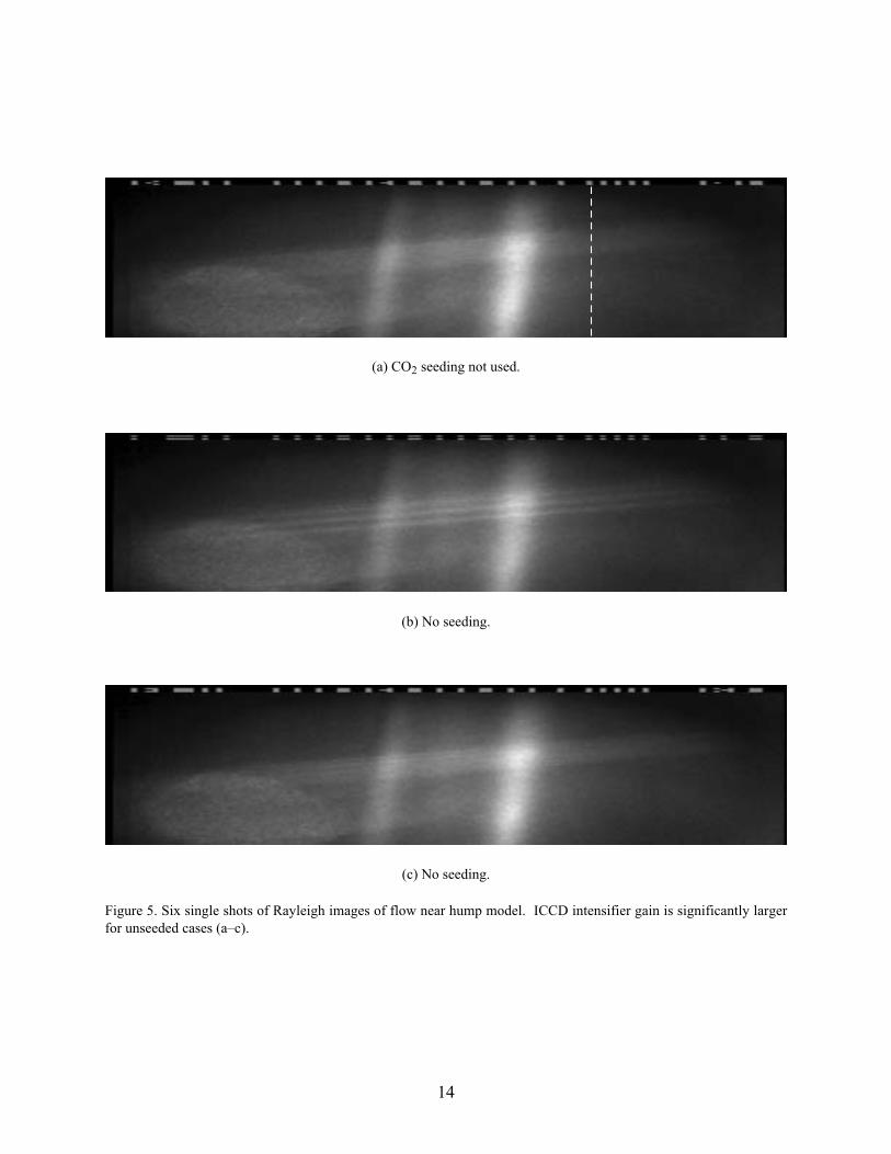
The perturbations to the light sheet are illustrated in figure 5, with the facility running at free-streamconditions: Mach 0.2, 3 × 105 Pa, 150 K. Six single-shot Rayleigh images are shown. Compare fig-ures 5(a)–5(c) (unseeded) with figures 6(d)–6(f) (CO2 seeding) to see the improvement in image qualitywith seeding. The broad vertical lines in figures 5(a)–5(c), stray scattered light off the model, are elimi-nated in the seeded cases of figures 5(d)–5(f) because the scattered signal from the light sheet is larger,relative to the scatter from the model surfaces. In spite of this significant perturbation (streaking) to thelaser beam, we tried to use these light sheets to observe fluid injection with the hump model.

Application to Oscillatory Excitation

Boundary layer control, including the prevention or delay of flow separation from a confining surface,has been studied for many years. Steady blowing, steady suction, and oscillatory excitation are threetechniques that are used. Early work (refs. 8 and 9) with oscillatory excitation at low Reynolds numberwas followed by demonstrations (ref. 10) at higher Reynolds numbers in the TCT. Recently, flow over anairfoil was simulated (ref. 6) by mounting a hump on the vertical wall of an otherwise empty tunnel (seefig. 1). This setup was designed to study oscillatory excitation and its effect on flow separation at free-stream conditions of Mach 0.2, 150 K, and 5 × 105 Pa.

To demonstrate an application of planar Rayleigh imaging in the TCT, we used this hump model tovisualize the flow just downstream of the slot S2, looking for transient flow features (e.g., vortex shed-ding) that may result from the oscillatory excitation through the slot. The ratio for the densities of thecolder free-stream fluid and the warmer fluid injected through the slot S2 is two, thus we expect, at best, afactor of two for the fractional change in density ∆ρ/ρ across the vortex of mixing fluid near the injectionslot. This density gradient should be detectable without seeding, based on the detection limit givenabove.

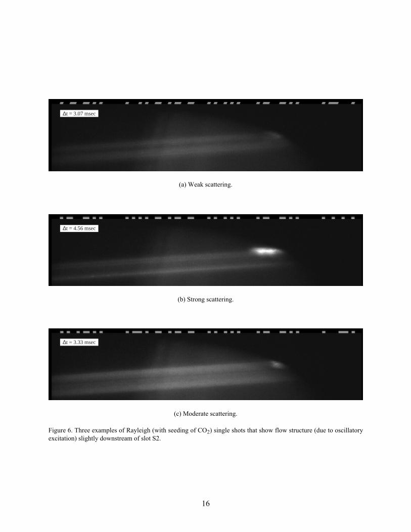
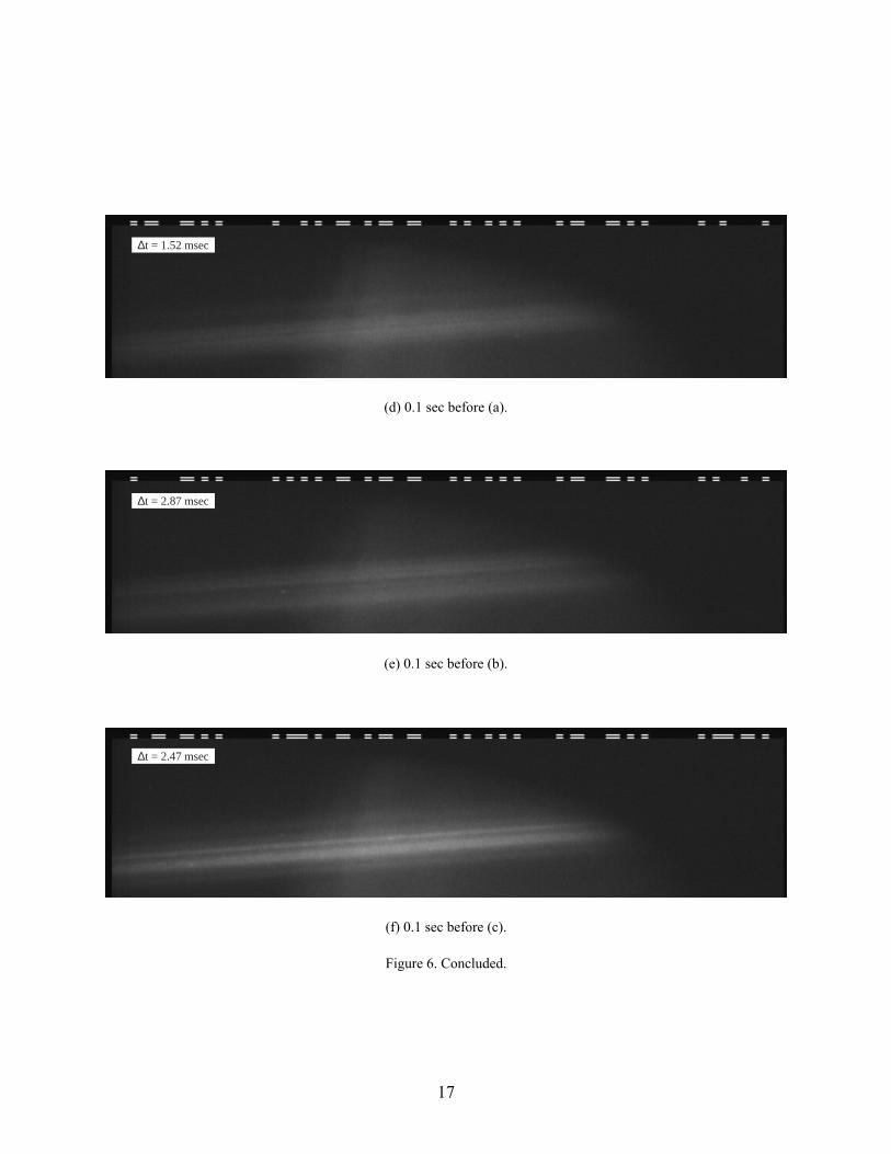
Figure 6 contains three instantaneous images (using CO2 seeding) showing three different instancesof transient flow structure due to weak oscillatory excitation. These three cases come from a larger set of44 laser shots, where the other 41 shots show no sign of flow structure. The figure 6(a) image shows asingle laser shot that contains a weakly scattering feature. The figure 6(b) image shows another single-pulse example of flow structure (much stronger than in fig. 6(a)) in the same location, and figure 6(c)shows a third moderately scattering structure. The position of these three features is about 1–2 cm (orless) off the wall and is shown by the small shaded ellipse within the camera’s field-of-view (dottedrectangle) in figure 2(a). For reference, images (figs. 6(d), 6(e), and 6(f)) show the laser shots immedi-ately before (0.1 sec) each of the shots used for figures 6(a)–6(c), respectively. All three reference imagesshow no observable feature.

The timing of the three examples of flow features shown in figures 6(a)–6(c) provides evidence thatthe observed features are due to the oscillatory excitation. All three occur at approximately the samerelative time with respect to the maximum pressure in the hump model cavity. The time delay ∆t is ameasure of the time between the maximum of the pressure pulse inside the model and the laser pulse andis specified in the figure for each of the six images. The frequency of oscillatory excitation for the data offigure 6 is 205 Hz; thus, the period is 5 msec, and we expect unsteady fluid flow with this same period.

7

Images (a) through (c) in figure 6 that contain the features have delays in the range of 3–4.5 msec, whilethe reference images (d) through (f), without features, have delays in the range of 1.5–3 msec. Thus,these six images are self consistent in the sense that all three possible flow structures appear in the samehalf of phase space, while all three reference images, without flow structure, are representative of theopposite half (i.e., ~180° out of phase). This result is consistent with an expectation of seeing somethingduring only one half of the oscillatory excitation period.

Degradation of the Laser Light Sheet

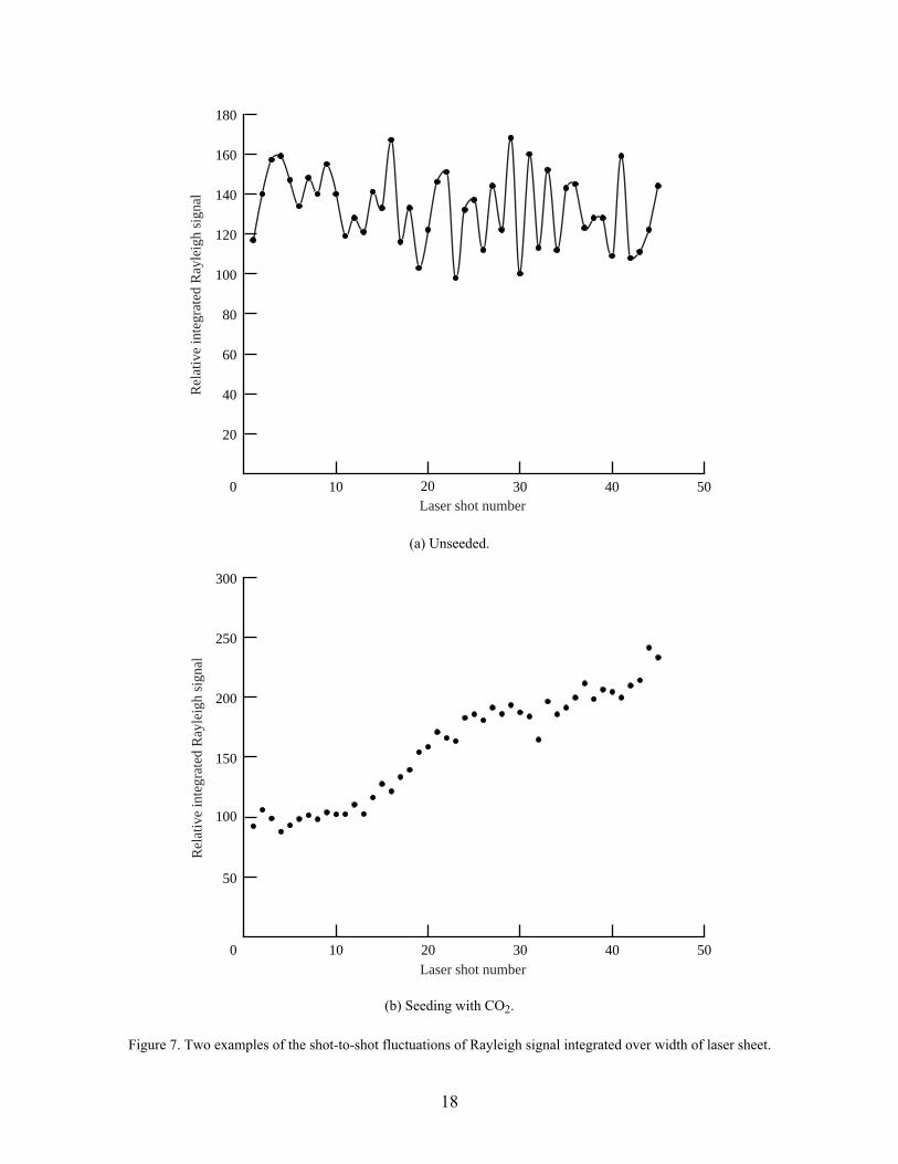
The streaking of the light sheet that was observed throughout the test, when the facility was runningwith typical cryogenic conditions, is likely generated by the fluid inside the tunnel since it is not evidenton the diode array data. These streaks are not due to absorption or attenuation of the laser beam inside thewind tunnel. To test for absorption, we calculate the integrated signal over the laser sheet width for eachlaser pulse. In figure 5(a), a dotted vertical line shows the column (i.e., position) where this integration iscarried out. Figure 7 shows two examples ((a) no seeding and (b) seeding of CO2) of integrating over theprofile of the light sheet at this particular location. Each data point in the figures is the result of integra-tion over the sheet width for one laser shot, with the background subtracted. Each figure shows theresults for a series of 44 successive laser shots (i.e., 4.4 sec of data). Because the signal with seeding ismuch greater than the signal without seeding, the camera gain is reduced for the case of figure 7(b) com-pared to figure 7(a).

The unseeded data of figure 7(a) show that the integrated signal (over the sheet width) is constant withlaser shot number or time and that the shot-to-shot variations are about 20 percent. This percentage isgreater than the pulse-to-pulse variations in the pulse energy, which were measured to be 10 percent whenusing the integrating sphere and photodiode. The signal variations are larger because the small Rayleighsignal contains stray background and shot noise. The seeded data of figure 7(b) show a steady increase inthe signal level. This steady increase is due to an increase in CO2 seed density over 4.4 sec. In this setup,we have only crude adjustment of the seed rate and cannot easily control the temporal stability of theseeded signal. However, over short time periods (~0.5 sec) containing several pulses, the data show thatthe integrated signal is roughly constant, whereas the streaks in figure 5 are changing every pulse. Thus,for both unseeded and seeded conditions, the total integrated light-sheet energy is not changing on apulse-to-pulse basis. Thus, the streaks arise with beam steering from index of refraction perturbations andnot from absorption.

Four possible causes for index of refraction variations are noted. First, assuming isentropic Mach 0.2flow and a recovery factor of one, the fractional density gradients in the test section would be dρ/ρ ≤1 percent, if the flow were completely stagnated. It is unlikely that these small density gradients couldcause the large effects seen in figures 5 and 6.

Second, did the slot S1 that was cut between the test section and the plenum cause boundary layerperturbations and hence the beam fluctuations of figure 5? The plenum pressure is typically <2 percentlarger than the test-section pressure. With the slot S1, a weak jet is created from the plenum into the testsection; however, the density gradients in this jet are also small and unlikely to cause the intense striationsin figures 5 and 6. Additionally, in previous (ref. 3) work, we observed excessive beam steering of a laserbeam (not a light sheet) without cutting holes in the test section walls (i.e., with windows on both sides ofthe test section) in this same facility.

8

A third possibility is temperature gradients in the plenum. Previous work (ref. 11) attributed thermalgradients in the plenum as the cause of image distortion in flow visualization at the TCT. This cause isroughly consistent with the streaking of figures 5 and 6.

A fourth possibility is the turbulent boundary layer region of the test section. If the perturbation is as-sumed to occur over a very short (localized) distance of path length, it is easy to visualize the generationof approximately parallel streaks, as seen in figures 5 and 6. The boundary layer at slot S1 is a likelycandidate for this region. The effect of this perturbation is then observed downstream in the laser sheetnear the model. What could provide the index-of-refraction variation necessary to steer the beam? Overthe course of this work and previous (ref. 3) work, we have observed a trend. Whenever the cryogenicflow is stagnated, we observe the generation of clusters in the fluid with Rayleigh instrumentation.Although we cannot conceive of a thermodynamic argument that predicts cluster formation in the bound-ary layer, we speculate that the boundary layer, which is effectively stagnated, may also contain sufficientclusters to provide the necessary index-of-refraction gradients to steer the beam. There is a second possi-bility related to clustering. In previous work (ref. 3), we typically observed clusters in the plenum, eventhough the free stream was free of clusters. Possibly, clusters are simply being sucked through slot S1into the test section boundary layer region.

Summary of Results

1. Off-body flow visualization of density, with planar Rayleigh scattering, was performed in theunseeded 0.3-Meter Transonic Cryogenic Tunnel (TCT).

2. Planar Raman imaging was also shown to be feasible in the unseeded TCT.

3. By seeding CO2 into the flow, clustering was induced and provided a significant enhancement ofthe Rayleigh flow visualization.

4. Planar Rayleigh imaging with seeding was used to observe transient flow structure due to vortexshedding in the wake of an oscillatory blowing slot.

5. The cryogenic fluid perturbs the intensity profile of the laser light sheet with streaks and degradesthe quality of the flow visualization.

9

References

1. Herring, G. C.; and Hillard, Jr., M. E.: Flow Visualization by Elastic Light Scattering in the Boundary Layer ofa Supersonic Flow. NASA TM-210121, Aug. 2000.

2. Escoda, M. C.; and Long, M. B.: Rayleigh Scattering Measurements of the Gas Concentration in TurbulentFields, AIAA Journal, vol. 21, 1983, pp. 81–84.

3. Shirinzadeh, B.; and Herring, G. C.: Demonstration of Imaging Flow Diagnostics Using Rayleigh Scattering inLangley 0.3-Meter Transonic Cryogenic Tunnel. NASA TM-208970, Feb. 1999.

4. Eckbreth, A. C.: Laser Diagnostics for Combustion Temperature and Species. Abacus (Cambridge, MA) 1988,Chapter 5.

5. Balakriskna, S.; and Kilgore, W. A.: Performance of the 1/3-Meter Transonic Cryogenic Tunnel with Air,Nitrogen, and Sulfur Hexafluoride Media Under Closed Loop Control. NASA CR-195052, Jan. 1995.

6. Seifert, A.; and Pack, L. G.: Active Control of Separated Flows on Generic Configurations at High ReynoldsNumbers. AIAA 99-3403, June–July 1999.

7. Shirinzadeh, B.; Balla, R. Jeffrey; and Hillard, M. E.: Rayleigh Scattering in Supersonic Facilities.AIAA 96-2187, June 1996.

8. Katz, Y.; Nishri, B.; and Wygnanski, I.: The Delay of Turbulent Boundary Layer Separation by OscillatoryActive Control. Phys. Fluids A, vol. 1, 1988, pp. 179–181.

9. Seifert, A.; Bachar, T.; Koss, D.; Shepshelovich, M.; and Wygnanski, I.: Oscillatory Blowing: A Tool to DelayBoundary-Layer Separation. AIAA Journal, vol. 31, 1993, pp. 2052–2060.

10. Seifert, A.; and Pack, L. G.: Oscillatory Control of Separation at High Reynolds Numbers. AIAA-98-0214, Jan.1998.

11. Snow, W. L.; Burner, A. W.; and Goad, W. K.: Improvement in the Quality of Flow Visualization in the Langley0.3-Meter Transonic Cryogenic Tunnel. NASA TM-87730, 1986.

10

ICCDcamera

Hump model mountedon tunnel side wall

Dichroicmirror M2

Oscillatoryexcitation

slot S2

Portion oflight sheet

within fieldof view

Diverging laserlight sheet

Free-stream

flow

θ

θ

Figure 1. Overview of planar light scattering at the 0.3-Meter Transonic Cryogenic Tunnel (TCT). (ICCD stands forintensified, charge-coupled device.)

11

Low pressureexhaust

High pressuresupply

3-way rotary valve

Photodiode

Test section

Flow

Plenum

S1

S2

W1

W2

M2

N.D. 3.0absorber

Integratingsphere

Lineardiodearray

BS2

BS1

Plenum

Hump

θ

L3L2

L1

(a) Top view.

W1

M4

L6

L5L4

M3

W2

High pressure,cryogenic plenum

Test section

Imaged laser sheet

ICCDcamera

Humpmodel

φ

(b) End view.

Figure 2. Schematic of the experimental setup at the TCT.

12

Raman light sheet

(a) Raman light sheet.

Rayleigh light sheet

(b) Rayleigh light sheet.

Figure 3. Examples of averaged (44 shots) images for (a) Raman and (b) Rayleigh light sheets in laboratory room airusing setup equivalent to TCT setup.

13

.2

.4

.6

.8

1.0

1.2

1.4

Transverse position, cm

Rel

ativ

e be

am in

tens

ity

.5 1.0 1.5 2.0 2.5 3.0 3.5 4.00

Figure 4. Single-pulse intensity profile across width of laser light sheet, measured on diode array while tunnel isrunning under typical conditions.

14

(a) CO2 seeding not used.

(b) No seeding.

(c) No seeding.

Figure 5. Six single shots of Rayleigh images of flow near hump model. ICCD intensifier gain is significantly largerfor unseeded cases (a–c).

15

(d) With CO2 seeding.

(e) With seeding.

(f) With seeding.

Figure 5. Concluded.

16

∆t = 3.07 msec

(a) Weak scattering.

∆t = 4.56 msec

(b) Strong scattering.

∆t = 3.33 msec

(c) Moderate scattering.

Figure 6. Three examples of Rayleigh (with seeding of CO2) single shots that show flow structure (due to oscillatoryexcitation) slightly downstream of slot S2.

17

∆t = 1.52 msec

(d) 0.1 sec before (a).

∆t = 2.87 msec

(e) 0.1 sec before (b).

∆t = 2.47 msec

(f) 0.1 sec before (c).

Figure 6. Concluded.

18

20Laser shot number

10 30 40 500

20

40

60

80

100

120

140

160

180

Rel

ativ

e in

tegr

ated

Ray

leig

h si

gnal

(a) Unseeded.

20 30 40 50

50

100

150

200

250

300

Laser shot number

Rel

ativ

e in

tegr

ated

Ray

leig

h si

gnal

100

(b) Seeding with CO2.

Figure 7. Two examples of the shot-to-shot fluctuations of Rayleigh signal integrated over width of laser sheet.

Form ApprovedOMB No. 0704-0188

Public reporting burden for this collection of information is estimated to average 1 hour per response, including the time for reviewing instructions, searching existing data sources,gathering and maintaining the data needed, and completing and reviewing the collection of information. Send comments regarding this burden estimate or any other aspect of thiscollection of information, including suggestions for reducing this burden, to Washington Headquarters Services, Directorate for Information Operations and Reports, 1215 JeffersonDavis Highway, Suite 1204, Arlington, VA 22202-4302, and to the Office of Management and Budget, Paperwork Reduction Project (0704-0188), Washington, DC 20503.

1. AGENCY USE ONLY

(Leave blank)

2. REPORT DATE 3. REPORT TYPE AND DATES COVERED

4. TITLE AND SUBTITLE 5. FUNDING NUMBERS

6. AUTHOR(S)

7. PERFORMING ORGANIZATION NAME(S) AND ADDRESS(ES)

9. SPONSORING/MONITORING AGENCY NAME(S) AND ADDRESS(ES)

11. SUPPLEMENTARY NOTES

8. PERFORMING ORGANIZATIONREPORT NUMBER

10. SPONSORING/MONITORINGAGENCY REPORT NUMBER

12a. DISTRIBUTION/AVAILABILITY STATEMENT 12b. DISTRIBUTION CODE

13. ABSTRACT

(Maximum 200 words)

14. SUBJECT TERMS

17. SECURITY CLASSIFICATIONOF REPORT

18. SECURITY CLASSIFICATIONOF THIS PAGE

19. SECURITY CLASSIFICATIONOF ABSTRACT

20. LIMITATIONOF ABSTRACT

15. NUMBER OF PAGES

16. PRICE CODE

NSN 7540-01-280-5500 Standard Form 298 (Rev. 2-89)

Prescribed by ANSI Std. Z39-18298-102

REPORT DOCUMENTATION PAGE

June 2002

Technical Memorandum

Flow Visualization of Density in a Cryogenic Wind Tunnel Using PlanarRayleigh and Raman Scattering WU 706-31-11-01

Gregory C. Herring and Behrooz Shirinzadeh

L-18171

NASA/TM-2002-211630

Using a pulsed Nd:YAG laser (532 nm) and a gated, intensified charge-coupled device, planar Rayleigh andRaman scattering techniques have been used to visualize the unseeded Mach 0.2 flow density in a 0.3-metertransonic cryogenic wind tunnel. Detection limits are determined for density measurements by using bothunseeded Rayleigh and Raman (

N

2

vibrational) methods. Seeding with CO

2

improved the Rayleigh flow visual-ization at temperatures below 150 K. The seeded Rayleigh version was used to demonstrate the observation oftransient flow features in a separated boundary layer region, which was excited with an oscillatory jet. Finally, asignificant degradation of the laser light sheet, in this cryogenic facility, is discussed.

Rayleigh scattering; Raman scattering; Cryogenic Wind Tunnel

23

NASA Langley Research CenterHampton, VA 23681-2199

National Aeronautics and Space AdministrationWashington, DC 20546-0001

Unclassified—UnlimitedSubject Category 74 Distribution: StandardAvailability: NASA CASI (301) 621-0390

Unclassified Unclassified Unclassified UL