FLOW OVER OBLIQUE WEIRS - Semantic Scholar€¦ · phenomena like hydraulic jump, undulation, flow...
159
FLOW OVER OBLIQUE WEIRS Final report -40 -20 0 20 40 60 80 100 120 -40 -20 0 20 0 10 20 TU Delft, October 2006 MSc. Thesis Nguyen Ba Tuyen Section of Hydraulic Engineering Faculty of Civil Engineering and Geosciences Graduation committee Prof. Dr. Ir. M.J.F. Stive Dr. Ir. W.S.J. Uijttewaal Prof. Dr. Ir. G.S. Stelling Ir. H.J. Verhagen Ir. R.J. Labeur
Transcript of FLOW OVER OBLIQUE WEIRS - Semantic Scholar€¦ · phenomena like hydraulic jump, undulation, flow...
FLOW OVER OBLIQUE WEIRSFinal report
-40-20
020
4060
80100
120
-40
-20
0
200
10
20
TU Delft, October 2006
MSc. ThesisNguyen Ba TuyenSection of Hydraulic EngineeringFaculty of Civil Engineering and Geosciences
Graduation committeeProf. Dr. Ir. M.J.F. StiveDr. Ir. W.S.J. UijttewaalProf. Dr. Ir. G.S. StellingIr. H.J. Verhagen
Ir. R.J. Labeur
- ii -
Master of Science Thesis:
FLOW OVER OBLIQUE WEIRSDraft report.
Name:
Nguyen Ba TuyenDate:
October 2006
Graduation committee:
Prof. Dr. Ir. M.J.F.Stive Section of Hydraulic Engineering
Dr. Ir. W.S.J. Uijttewaal Section of Environmental Fluid Mechanics
Prof. Dr. Ir. G.S.Stelling Section of Environmental Fluid Mechanics
Ir. H.J.Verhagen Section of Hydraulic Engineering
Ir. R.J. Labeur Section of Environmental Fluid Mechanics

- iii -
ACKNOWLEDGEMENTS
The experimental and theoretical study on flow over oblique weirs is the subject of myMaster of Science Thesis. This is the most important part that is required for the MScdegree of Civil Engineering and Geosciences at Delft University of Technology. The studywas conducted at the Fluid Mechanics Laboratory (Stevin III Laboratory) – TU Delft.
First of all I would like to express my deep appreciation of the thorough provision andguidance provided by Dr.Ir. W.S.J. Uijttewaal. During the last year, I have learned a lotfrom his inspiring guidance and enthusiastic daily work. I wouldn’t have overcome mymistakes and faults without his help. I am also grateful to Prof. Dr.Ir. M.J.F. Stive, Dr.Ir.H.L. Fontijn, and Ir. H.J. Verhagen and for their valuable advices during the first steps,which is also the foundation of this work.
I would like to thank all the members of my thesis committee for sharing their knowledgeand experiences, for their guidance and judgement. Special thank to Prof. Dr. Ir. Stellingfor the introduction of his theoretical analyses on flow over weirs in submerged condition,on which is computational simulations are based.
Many thanks also to S. de Vree, J.A. van Duin, H. Tas and the laboratory staff; B.A. Wols,H. Talstra, W.A. Breugem, E.A. van Blaaderen and my colleagues for providing thenecessary facilities and guidance for conducting my work. The devotion of S. de Vree andthe always-positive feedbacks from B.A. Wols greatly contributed to my final thesis.
Last but not least, I would like to acknowledge the sponsors CICAT and TUDELFT, underthe framework of CE-HWRU project, for their financial and other valuable supports duringthe time I have been living and studying in Delft. Great thanks to my family and friends forbeing a firm moral support and source of encouragement.
Nguyen Ba TuyenTU Delft, October 2006

- iv -
ABSTRACT
This report is the conclusion of a comprehensive set of experiments, which wereperformed on weirs placed obliquely in an open channel. Its purpose is to report onlaboratory investigation on the flow over different types of oblique weirs, including behaviorand hydraulic characteristic of the flow, different phenomena in the neighborhood of theweir, and hydraulic parameters and physical laws that govern the process. The report alsoaims at presenting a quantitative view on the energy loss and the discharge coefficient foroblique weirs.
To that end, many experiments were performed in a shallow flume under various flowconditions. Three different types of impermeable weirs are tested, namely a rectangularsharp-crested weir, a rectangular broad-crested weir (both placed 45 degrees obliquely tothe flow direction) and a dike-form weir with both upstream and downstream slopes of 1:4.The last type was tested with several oblique angles of 0, 45 and 60 degrees with theincident flow.
By adjusting the flow discharge and the downstream water level, different flow regimesand states reveal the complex three dimensional structure of the flow with variousphenomena like hydraulic jump, undulation, flow concentration, flow divergence, gyreformation, etc. In case of emerged flow condition, the flow behind weir becomes highlyturbulent and very complex, which make it more difficult to perform accuratemeasurements. This flow regime also accounts for the higher head loss and energydissipation than in case of submerged flow. Generally speaking, the hydraulic phenomenathat happen in the neighborhood of an oblique weir are equivalent for different weir form,although there are some remarkable differences such as the size of the recirculation zonebehind weir, and the amplitude of the undulation waves.
Experimental data were obtained by many instruments and techniques; most of them hadbeen carefully calibrated and were highly accurate and reliable. The data collected fromacoustic and electro-magnetic single point velocimeters and depth measurements wereused to investigate the hydraulic process and the phenomena of interest. Meanwhile thewhole surface flow velocity field was measured using particle tracking velocimetrytechnique, which helps obtaining instantaneous whole field velocity maps. Combine withmathematic tools we can interpret the data and gain necessary statistical information.
When the oblique angle of the weir is altered, both the flow direction and the flow ratechange. The flow always tends to keep its direction to nearly perpendicular to the weircrest when it reaches and passes the weir. This leads to the difference in water levels attwo ends of the weir, the flow concentration at on one side of the flume behind weir, thevariation in flow velocity distribution and other asymmetries across the flow. Increasing theoblique angle, the effective length of the weir increases significantly, whereas thedischarge coefficient Cd slightly decreases. Together they make the discharge capacity ofthe oblique weir increases.
Finally, the discharge coefficient and its relations to other flow and geometry parametersobtained from this research were compared to the available knowledge on oblique weirs,including the published researches from De Vries (1959), Borghei et al. (2003) and thenumerical models simulations from Wols (2005). The common findings betweenresearches enhanced each other reliability; whereas the differences are a motivation forfurther studies.

- v -
TABLE OF CONTENTS
Final report.............................................................................................................................. iLIST OF FIGURE...............................................................................................................viiiLIST OF TABLES...............................................................................................................xiiLIST OF SYMBOLS ..........................................................................................................xiiiCHAPTER 1. INTRODUCTION ..................................................................................... 1
1.1. General................................................................................................................... 11.2. Problem description ............................................................................................... 21.3. Objective ................................................................................................................ 31.4. Research method.................................................................................................... 41.5. Domain of the study............................................................................................... 51.6. Outline of the thesis ............................................................................................... 5
CHAPTER 2. PHYSICAL BACKGROUND AND THEORY........................................ 62.1. Introduction............................................................................................................ 62.2. Flow in open channel ............................................................................................. 6
2.2.1. Basic concepts................................................................................................ 62.2.2. Resistance in the flow .................................................................................... 82.2.3. Turbulence and energy loss ........................................................................... 9
2.3. Flow over plain weirs........................................................................................... 102.3.1. Introduction.................................................................................................. 102.3.2. Flow regimes................................................................................................ 102.3.3. Weir geometry ............................................................................................. 112.3.4. Energy loss with the present of weir............................................................ 122.3.5. Discharge coefficient - Cd and Cdv ............................................................... 122.3.6. Discharge formulas ...................................................................................... 132.3.7. Energy balance and Momentum balance ..................................................... 15
2.4. Flow over oblique weir ........................................................................................ 172.4.1. Oblique sharp crested weir........................................................................... 172.4.2. Oblique trapezoidal weir.............................................................................. 182.4.3. Numerical simulations on oblique weirs...................................................... 192.4.4. Theoretical analysis of the flow over an oblique weir ................................. 20Conclusion ................................................................................................................... 23
CHAPTER 3. SET-UP AND IMPLEMENTATION OF EXPERIMENTS ................... 243.1. Introduction.......................................................................................................... 243.2. Experimental parameters ..................................................................................... 24
3.2.1. Choosing experiment parameters................................................................. 243.2.2. Dimensional analysis, scaling and similitude .............................................. 25
3.3. Design of weirs .................................................................................................... 273.3.1. Sharp crested weir:....................................................................................... 273.3.2. Broad crested weir: ...................................................................................... 273.3.3. Dike form weirs: .......................................................................................... 27
3.4. Major experimental equipments .......................................................................... 283.4.1. Measurement site ......................................................................................... 283.4.2. Point gauges ................................................................................................. 283.4.3. Manometer with flange ................................................................................ 293.4.4. ADV – Acoustic Doppler Velocimeter ........................................................ 293.4.5. EMF – Electro Magnetic Flow meter .......................................................... 30

- vi -
3.4.6. Facilities for PTV analysis........................................................................... 313.5. Measurements elaboration ................................................................................... 32
3.5.1. PTV measurement........................................................................................ 323.5.2. Loss measurement........................................................................................ 323.5.3. Velocity measurement ................................................................................. 33
3.6. Whole field measurements with PIV and PTV.................................................... 343.6.1. General......................................................................................................... 343.6.2. PTV processing procedure........................................................................... 353.6.3. Calibration.................................................................................................... 363.6.4. Further investigations................................................................................... 373.6.5. Limits ........................................................................................................... 38
3.7. Accuracy and tolerance of measurements............................................................ 383.7.1. Water depth.................................................................................................. 383.7.2. Velocity........................................................................................................ 383.7.3. Discharge ..................................................................................................... 39
CHAPTER 4. RESULTS AND ANALYSIS OF............................................................ 40LOSS MEASUREMENTS .................................................................................................. 40
4.1. Loss measurements with plain weir..................................................................... 404.1.1. Present losses by flow condition .................................................................. 404.1.2. Analysis of losses......................................................................................... 42
4.2. Loss measurements on oblique weirs .................................................................. 464.2.1. Present loss by flow condition ..................................................................... 464.2.2. Analysis of loss measurement...................................................................... 49
CHAPTER 5. RESULT AND ANALYSIS .................................................................... 56OF VELOCITY MEASUREMENTS.................................................................................. 56
5.1. Introduction.......................................................................................................... 565.2. Surface flow velocity field ................................................................................... 56
5.2.1. Perpendicular weir (= 00).......................................................................... 575.2.2. 450 oblique weir ........................................................................................... 595.2.3. 600 oblique weir ........................................................................................... 655.2.4. Flow velocity far downstream of the weir ................................................... 66
5.3. Vertical profiles of velocities............................................................................... 695.3.1. Illustration of velocity profiles over flow depth .......................................... 695.3.2. Velocity measurement along the flume ....................................................... 705.3.3. Three dimensional flow structure ................................................................ 725.3.4. Analysis of the flow structure ...................................................................... 735.3.5. The recirculation zone.................................................................................. 75
5.4. Two velocity component analysis........................................................................ 765.4.1. Velocity variation along the flow ................................................................ 765.4.2. Velocity variation across the flow ............................................................... 785.4.3. Spatial (2D) variation of the velocity components ...................................... 78
5.5. Angle of obliqueness............................................................................................ 805.5.1. General......................................................................................................... 805.5.2. Oblique trapezoidal weir, = 450 ................................................................ 825.5.3. Oblique trapezoidal weir, = 600 ................................................................ 83
CHAPTER 6. DISCUSSION.......................................................................................... 856.1. General structure and behavior of the flow.......................................................... 856.2. Discussions on the discharge coefficients............................................................ 86
6.2.1. The compatibility of available empirical formulas for Cd ........................... 866.2.2. Comparison of results from this research with data from De Vries ............ 87
- vii -
6.2.3. Comparison of results from this research with data from Stelling .............. 896.3. Projected discharge coefficient ............................................................................ 89
CHAPTER 7. CONCLUSIONS...................................................................................... 937.1. Conclusions.......................................................................................................... 937.2. Feasibility of this study and further research ....................................................... 94
7.2.1. Accomplishments of this study.................................................................... 947.2.2. Recommendations........................................................................................ 94
REFERENCES .................................................................................................................... 96APPENDICES ...................................................................................................................- 1 -
APPENDIX A: THEORETICAL ISSUES....................................................................- 2 -A.1. Turbulence in the flow and Reynolds stresses ...................................................- 2 -A.2. Dimensional analysis, modeling and similitude ................................................- 3 -A.3. A simple flow model ..........................................................................................- 4 -
APPENDIX B: LOSS MEASUREMENTS AND ANALYSIS ..................................- 11 -B.1. Trapezoidal weir,= 00 ..................................................................................- 11 -B.2. Trapezoidal weir,= 450 ................................................................................- 13 -B.3. Trapezoidal weir,= 600 ................................................................................- 15 -
APPENDIX C: VELOCITY MEASUREMENTS AND ANALYSIS........................- 17 -C1. Processing procedure from raw image to time-averaged velocity vector field.- 17 -C2. Analyses of the velocity vector field.................................................................- 20 -
APPENDIX D: MAJOR MATLAB SCRIPTS ...........................................................- 25 -D.1. theorymain.m ...................................................................................................- 26 -D.2. theorypro.m......................................................................................................- 27 -D.3. ImportDataF.m.................................................................................................- 28 -D.5. ADVpro.m........................................................................................................- 30 -D.6. PlotFigures.m ...................................................................................................- 31 -D.7. weirmain.m ......................................................................................................- 33 -D.8. weirpro.m .........................................................................................................- 35 -D.9. tuyen_calib.m...................................................................................................- 36 -D.10. calibratePTV.m ..............................................................................................- 37 -D.11. sline.m............................................................................................................- 38 -D.12. extract1diagonal.m.........................................................................................- 39 -D.13. extract1streamline.m......................................................................................- 41 -D.14. extract1horizontal.m ......................................................................................- 42 -D.15. obliqueangle.m...............................................................................................- 43 -D.16. AnglePrediction.m .........................................................................................- 45 -D.17. AnglePrediction 4560.m ................................................................................- 47 -
APPENDIX E: ARCHIVES OF DATA ......................................................................- 49 -
- viii -
LIST OF FIGURE
Figure 1.1: The flow over an oblique weir and its relating phenomenaFigure 1.2: Typical cross section of big rivers in the Netherlands
Figure 2.1: Definition sketch of open channel flowFigure 2.2: The specific energy diagramFigure 2.4: The convention of parametersFigure 2.5: Four main types of flowFigure 2.6: Sharp-crested weir geometryFigure 2.7: Broad-crested weir geometryFigure 2.8: Definition of flow zonesFigure 2.9: The relation between C* and S, p=525.Figure 2.10: Cd as a function of Fr1.Figure 2.11: The submergence as a function of Fr1.Figure 2.12: Plan view of an oblique weir.Figure 2.13: Free flowFigure 2.14: Submerged flowFigure 2.15: De Vries experimentFigure 2.16: Streamlines show the spiral recirculation movement of flow downstream anoblique weir (450). An illustration from simulations Wols (2005).Figure 2.17: Velocity component analysisFigure 2.18: Upstream energy balanceFigure 2.19: Relation between the flow direction and flow condition above the weirFigure 2.20: Relation between the flow direction and oblique angle of the weir
Figure 3.1: The experiment site in the Laboratory.Figure 3.2: Sharp crested weirFigure 3.3: Broad crested weirFigure 3.4: Dike-form weirFigure 3.5: Schematized plan view of the flume and its apparatusFigure 3.6: The instrument carriageFigure 3.7: Manometer with Pitot tube.Figure 3.8: The Vectrino probeFigure 3.9: Typical arrangement of the ADV and the bubble generator.Figure 3.10: The xyz coordinate of the instrumentFigure 3.11: The flow seeded with black tracers.Figure 3.12: Head loss measurement pointsFigure 3.13: Positioning velocity measurement pointsFigure 3.14: Measurement points over the flow depth.Figure 3.15: Sliding image processFigure 3.16: Cross-correlation makes instantaneous velocity vector field imageFigure 3.17: Velocity vector fieldFigure 3.18: The streamlinesFigure 3.19: The velocity variation along a streamline

- ix -
Figure 4.1: Relation between head loss and Froude number above the weir, = 00
Figure 4.2: Relation between head loss and the relative downstream water depth, = 00
Figure 4.3: Cd, C* and fit curves for C* by VillemonteFigure 4.4: Relation between Cd and submergence, =00, Q=30l/sFigure 4.5: Relation between fit parameter and dischargeFigure 4.6: Relation between discharge coefficient and Froude number above the weir, =0Figure 4.7: Relation between submergence and Froude number above the weir, = 00
Figure 4.8: Relation between discharge coefficient and the relative upstream head, = 00
Figure 4.9: Relation between discharge Cdv and other parameters,= 00
Figure 4.10: Relation between head loss and Froude number above the weirFigure 4.11: Relation between Fr1 and the relative downstream water depthRelation between head loss and the relative downstream water depthFigure 4.12: Measurement data for Cd, C* and Ks with different oblique weirs.Figure 4.13: Relation between discharge coefficient and Froude number above the weirFigure 4.14: Relation between submergence and Froude number above the weirFigure 4.15: Relation between discharge coefficient and the relative upstream headFigure 4.16: Discharge coefficient with different oblique angles
Figure 5.1: Flow velocity vector field,=00 , Q=30l/s, Emerged flowFigure 5.2: Flow velocity vector field,=00 , Q=30l/s, Undulated flowFigure 5.3: Flow velocity vector field,=00 , Q=25l/s, Submerged flowFigure 5.4: Variation of the total velocity,=00, Q=25l/s, Submerged flowFigure 5.5: Flow velocity vector field, trapezoidal weir,=450, Q=30l/s, Emerged flowFigure 5.6: Flow velocity vector field, trapezoidal weir,=450, Q=30l/s, Undulated flowFigure 5.7: Flow velocity vector field,=450 , Q=30l/s, Submerged flowFigure 5.8: Variation of the total velocity,=450, Q=30l/s, Undulated flowFigure 5.9: Flow velocity field for sharp crested weir, =450, Q=35l/sFigure 5.10: Velocity along the middle streamline, =450, Q=35l/s, undulated flowFigure 5.11: Flow velocity field for broad crested weir,=450, Q=35l/sFigure 5.12: Velocity along the middle streamline, =450, Q=35l/s, emerged flowFigure 5.13: Velocity along the middle streamline, =450, Q=35l/s, undulated flowFigure 5.14: Standing wave on top of a broad-crested weir, =450, Q=35l/sFigure 5.15: Flow velocity vector field,=600 , Q=40l/s, Emerged flowFigure 5.16: Flow velocity vector field,=600 , Q=35l/s, Undulated flowFigure 5.17: Flow velocity vector field, =600 , Q=40l/s, Submerged flowFigure 5.18: Variation of the total velocity,=600, Q=20l/s, Undulated flowFigure 5.19: Downstream flow velocity vector field, =450, Q=30l/s, emerged flowFigure 5.20: Downstream flow separation, =450, emerged flowFigure 5.21: Downstream velocity distribution across the flume, =450, Q=30l/s, emergedflow.Figure 5.22: Downstream velocity distribution across the flume, =450, Q=30l/s,submerged flow.Figure 5.23: Velocity distribution over the flow depthFigure 5.24: Relation between U and z

- x -
Figure 5.25: Positioning the measurement pointsFigure 5.26: Surface flow velocity along the center streamlineFigure 5.27: Vertical velocity profiles at several sections downstream of the weirFigure 5.28: Vertical velocity profiles, V and WFigure 5.29: Velocity variations along the streamline and over the depth.Figure 5.30: Velocity profiles on the downstream and on the slope of the weir.Figure 5.31: The left-right difference in water depth above the weirFigure 5.32: The recirculation zone behind a trapezoidal weir, q=0.15m2/sFigure 5.33: The recirculation zone behind a sharp-crested weir, q=0.15m2/sFigure 5.34: Velocity components analysis for different flow regimes.Figure 5.35: Velocity variation with different weir configurationsFigure 5.36: Velocity variation along the weir crestFigure 5.37: Spatial velocity distributionFigure 5.38: Spatial distribution of velocity componentsFigure 5.39: Spatial distribution of oblique angle, =450, Q=30l/s, submerged flowFigure 5.40: Spatial distribution of oblique angle, =450, Q=30l/s, undulated flowFigure 5.41: Chaos downstream of an oblique angle, =450, Q=30l/s, emerged flowFigure 5.42: Spatial distribution of oblique angle, =600, Q=40l/s, emerged flowFigure 5.43: Result of oblique angle analysis for the 450 oblique weirFigure 5.44: Relation among , and flow conditions.Figure 5.45: Result of oblique angle analysis for the 600 oblique weirFigure 5.46: Relation among , and flow conditions.
Figure 6.1: Relation between Cd and S by different formulas, = 450
Figure 6.2: Comparison of formulas from Borghei and VillemonteFigure 6.3: Comparison of discharge coefficientsFigure 6.4: Comparison of Cdv with several oblique angles from De Vries (1959).Figure 6.5: Figure 6.4: Comparison of Cdv for plain weirFigure 6.6: Velocity component parallel to the weir, =450, Q=30l/s, submerged flow.Figure 6.7: Variation of the perpendicular velocity component along the weir crest,
=450 , submerged flow.
Figure A1: The stress tensorFigure A2: Flow model with its parametersFigure A3: Cd(R) with and without bottom frictionFigure A4: Cd(R) for different specific dischargesFigure A5: Comparison of Cd(R) calculated by the complex method
and by the empirical formula of G.S.StellingFigure A6: Differences between flow parameters calculated by different methods
Figure C1: The flow seeded with black tracers (original image, captured by the camera)Figure C2: Ensemble-averaged picture (background picture)Figure C3: The subtracted pictureFigure C4: Instantaneous velocity vector fieldFigure C5: Fix-grid-points velocity vector fieldFigure C6: Fix-grid-points, time-averaged velocity vector field

- xi -
Figure C7: Velocity vector field with streamlinesFigure C8: Velocity variation a long one streamline (the center streamline)Figure C9: Variation of a velocity component a long the weir crestFigure C10: Variation of different velocity components a long a cross-sectionFigure C11: Spatial distribution of the total velocityFigure C12: Contours of different velocity componentsFigure C13: Contours of the angle of obliqueness of the flow
- xii -
LIST OF TABLES
Table 3.1: Experiment variables
Table 4.1: Measurement from experiment with Q = 40l/s, = 00.Table 4.2: Cdv with different discharges and different oblique angle
Table 5.1: Measurements of velocity profilesTable 5.2: Measurements points by the ADVTable 5.3: Extra measurements for oblique angle, = 450
Table 5.4: Extra measurements for oblique angle, = 600
Table B1: Loss measurements for trapezoidal weir, = 00.Table B2: Loss measurements for trapezoidal weir, = 450.Table B3: Loss measurements for trapezoidal weir, = 600.
Table D1: List of presented Matlab scripts

- xiii -
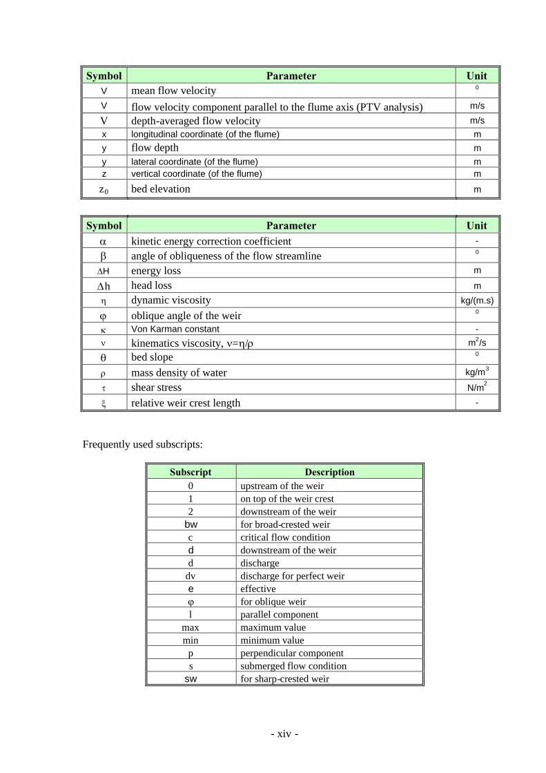
LIST OF SYMBOLS
Symbol Parameter UnitA area of the wet section of the flow m2
aw weir height m
B flume width (channel width) m
C Chezy resistance coefficient m1/2/s
C* discharge reduction coefficient -
Cd discharge coefficient -
Cdv dicharge coefficient for perfect weir (free flow or emerged flow) -
d water depth w.r.t the channel bottom m
d flow depth m
E specific energy m
f Weisbach resistance coefficientFr Froude number -
g gravitational acceleration m/s2
H total head m
h the water depth w.r.t. the weir crest m
i bottom slope -
K calibration factor (PTV analysis) -
Ks submergence coefficient -
L length of the weir m
Lw length of the weir crest (in the flow direction) m
m weir slope -
mk discharge coefficient for the weir -
ms discharge coefficient for the channel -
n Manning resistance coefficient
pfit parameter (Villemonte) [-]; atmospheric pressure [m]; reductionfactor of the discharge coefficient due to the obliqueness of the flow(De Vries) [-]
-
P wet perimeter of the flow m
Q total discharge m3/s
q specific discharge m2/s
R hydraulic radius m
Re Reynolds number -
S submergence; flow resistance slope (the energy slope or friction slope) -
Uflow velocity component perpendicular to the flume axis (PTVanalysis) m/s
u flow velocity m/s
u* the shear stress velocity m/s
- xiv -
Symbol Parameter UnitV mean flow velocity 0
V flow velocity component parallel to the flume axis (PTV analysis) m/s
V depth-averaged flow velocity m/sx longitudinal coordinate (of the flume) my flow depth my lateral coordinate (of the flume) mz vertical coordinate (of the flume) m
z0 bed elevation m
Symbol Parameter Unit kinetic energy correction coefficient -
angle of obliqueness of the flow streamline 0
H energy loss m
h head loss m
dynamic viscosity kg/(m.s)
oblique angle of the weir 0
Von Karman constant - kinematics viscosity, =/ m2/s
bed slope 0
mass density of water kg/m3
shear stress N/m2
relative weir crest length -
Frequently used subscripts:
Subscript Description0 upstream of the weir1 on top of the weir crest2 downstream of the weir
bw for broad-crested weirc critical flow conditiond downstream of the weird discharge
dv discharge for perfect weire effective for oblique weirl parallel component
max maximum valuemin minimum value
p perpendicular components submerged flow condition
sw for sharp-crested weir

MSc. Thesis Flow over Oblique weirs
Page 1
CHAPTER 1. INTRODUCTION
1.1. GeneralWeirs are among the most popular and simple hydraulic structures. They can be used forvarious purposes, from flow measurement and diversion, energy dissipation to regulationof flow depth, and many others. Weirs can be encountered in real life in various types andshapes, and they can sometimes be placed obliquely to the incident flow in order toincrease the efficiency. Besides, many obstacles in a flood plain can act as weirs during ahigh water period, for example the summer dikes, roads with high foundation, groynes orbarrages. In fact, those weir-like obstacles can hardly be considered as plain(perpendicular) weirs.
The characteristics and hydraulic behavior of plain weirs or standard weirs have beenstudied for a long time and the understanding on them is rather deep. We can easilycalculate the parameters of the flow using the conventional weir equations and formulae.However, few studies have been done on weirs placed obliquely in the flow. Sufficientinformation on the discharge coefficient, energy loss and other behaviors of the flow overan oblique weir is still not available. Up to now, there is no commonly accepted designdischarge equation for an oblique weir.
Probably the first rational approach to studying flow over oblique weirs was published byDe Vries in his report in Dutch (“Scheef aangestroomde overlaten”, April 1959). The mainobjective of the research was to examine the influence of the obliqueness of the weir to theflow. Experiments were done on trapezoidal weirs.
More recently, Borghei (2003) and his co-authors published their study on the dischargecoefficient for oblique rectangular sharp-crested weir. Their research demonstrated theinfluence of the oblique angle to the discharge coefficient Cd, resulting in a single formulafor Cd , and correction coefficients for submerged flow.
Since then, many researchers have investigated the weir discharge coefficient with themain channel upstream Froude number. However, sufficient information on the variation ofthe coefficients used in their equations is still not available. Up to now, there is nocommonly accepted design discharge equation for an oblique rectangular sharp crestedweir.
Furthermore, we need some more understanding of the physical processes that arepredominant in a flow over oblique weirs in various forms, which has hardly beendescribed or published. By means of qualitative description on what happens in the vicinityof oblique weirs, on the weir crest, and with flow structures down stream, this report triesto bring a fresh and further look for those interesting hydraulic phenomena. It also aims atquantitatively describing the absolute energy loss and discharge coefficients for the flowover oblique weirs. Experiments were performed on physical models of some commontypes of weir, including a sharp crested weir, a broad crested weir and trapezoidal weirsunder several different oblique angles. This research was done in the laboratory of Fluidmechanics, faculty Civil Engineering and Geosciences, Delft University of Technology.

MSc. Thesis Flow over Oblique weirs
Page 2
Flow
Obliquely placed weir Flow seperation
Stream linesDeflection of flow
Flow convergence
The flume
Circ
ulatio
n
Figure 1.1: The flow over an oblique weir and its relating phenomena
1.2. Problem descriptionThe recent high waters in the Netherlands, for example the flood in 1995, have raised anumber of matters in river flow and the concern of public about the security againstflooding. In 1996, the policy “Room for the river” had become effective, which aimed atincreasing the capacity of the large rivers and reducing the impact of high waters. Thetypical cross section of a river in the Netherlands often comprises of winter dike, summerdike and other constituents (see figure 1.2). Summer dikes are part of the foreland asmentioned in the dike law. Their main functions are water control (protection frominundation), restriction of morphological impacts by the outer flow, and accessibility(playing the role of roads). During the flooding periods, summer dikes however reduce thedischarge capacity of the river. The summer dikes will be overflowed under such extremedischarges, and part of the river discharge flow through the winter bed with several weir-like obstacles mentioned earlier. River managers are now seeking for the understanding ofdischarge capacity, energy loss and other characteristics of the flow concerning the summerdike and those obstacles. Generally speaking it has the form of a flow over an oblique weirbecause of the randomness in their orientation. However, the influence of the obliquenesson energy loss and flow rate has hardly been examined.
Built up areaAgriculture
Primari river dikeWinter dike Winter dike
Sidechannel
Summer dike
Groynes
Summer dike
Figure 1.2: Typical cross section of big rivers in the Netherlands
The above problem is also essential for Vietnam as our country has several big riversystems with their social-economically important flood plains. Especially in the South hub,where the great Mekong river has hardly any primary river dike protection, but a lot ofregional dikes, roads, structures and other obstacles.

MSc. Thesis Flow over Oblique weirs
Page 3
What is also important for Vietnam in the current situation is the safety of sea dikes and theflooding problems caused by storm surges. Researches on the damage of the Damreytyphoon, which landed in September 2005 to the Northern provinces of Vietnam, hasrevealed a fact that the design height of the sea dikes was too low that their failure was notonly due to wave run-up and over topping, but also because of over flowing. Thecombination of the shape of the local coast line, the current, storm surge, and tide make theflow over sea dikes, which can be interpreted as flow over weir, not always perpendicularto the dike axis. Research on flow over oblique weirs is an urged need from practice.
1.3. ObjectiveThe first purpose of this research is to qualitatively describe the structure of the flow oversome main types of oblique weirs and other complex phenomena related to it. The flow’sbehaviors, hydraulic characteristics, and their inter-relation are therefore the objectives ofinvestigation. We will also examine the physical processes which play a role, how theyinfluence the flow over an oblique weir, and if there are common laws that govern thisbehavior.
Secondly we need to quantitatively determine the energy loss and discharge coefficientconcerning the flow in those cases, i.e. to determine the absolute size of losses and theirsrelation with other flow and geometry parameters, especially the oblique angle. Those toserve drawing conclusions as to what respect the flow over an oblique weir deviates fromthe flow over a perpendicular weir. Finally the result will be checked with availableknowledge on flow concerning oblique weirs.
To express the purposes more specifically, the discharge coefficient Cd and its relation toother parameters is one of the main objectives. Variations of Cd under different obliqueangles need to be investigated. The experimentally determined correction factor Cd is usedto account for the energy loss not included in the simplified analysis to get the actualdischarge (Q) as a function of the water head upstream (H):
322 2
3dQ C B gH
The oblique angle of the flow streamlines over a weir is also the main object of theexperiments. The change in the direction of the flow in different flow regimes under theinfluence of several parameters is to be investigated. The relation between the obliqueangle of the flow streamlines (), the oblique angle of the weir (), and the Froude number(Fr) of the flow is especially interesting.
= f(, Fr0, Fr1)where Fr0 is the upstream Froude number, Fr1 is the Froude number above the weir crest.
Velocity components analysis contributes to the understanding of the physical process thatgoverns flows over an oblique weir. Earlier studies on oblique weirs have revealedinteresting facts that need to be checked and studied more detailed where possible. Besides,the flow downstream of an oblique weir has a complex three dimensional structures. Itshows many turbulence properties that contribute to the transfer and dissipation of energy.One example is the flow with a recirculation zone behind weir. These phenomena need tobe described qualitatively and their effects determined qualitatively.
MSc. Thesis Flow over Oblique weirs
Page 4
1.4. Research methodThe flow structure in the presence of a weir is generally three dimensional andcomplicated. In case the weir is placed obliquely, it becomes even more complex with avariety of interesting phenomena and their underlying physical laws. An approach to thisproblem is found through the use of a combination of analysis and experiments.
In order to achieve the main objectives of this study, we need to accurately measure theflow properties, examine the phenomena that happen in the neighborhood of the weir, andinvestigate the relationships between them. To effectively perform those tasks, we can takerefuge in modern instruments and techniques. One of those is the PTV (Particle TrackingVelocimetry) method with the capability of extracting the underlying flow velocity field. Ithelps giving us the instantaneous as well as the time averaged surface velocity vector mapsof the whole flow area concerning the weir. For further investigation into the flowstructure, an ADV (Acoustic Doppler Velocimeter) has been used for point measurementsof all three components of the velocity vector.
The PTV analysis mainly gives an overview of the free surface flow velocity field.However, the weir configurations and arrangements in the flume cause the flow to showthree-dimensional complexity, particularly downstream of the weir and under emergedflow conditions. In order to understand the flow characteristic and be able to describe itsstructure, we need additional information from other experimental techniques andmeasurement methods.
The flow can be represented by simple models, based on physic and basic equations: theenergy balance, momentum balance and continuity equations. Given the input parameters,the flow parameters of interest can be analytically determined. These outputs can be thewater depth, specific discharge, oblique angle, and many others. This kind of analysisproved to be indispensable during the course of this research. As mentioned earlier, therewas also a more extensive and sophisticated study on 3D computer modeling of flow overoblique weirs carried out by Wols (2005).
The comparison of experimental results with model outcomes is of importance in order tosee if the phenomena that occurred in the flume can be reproduced in the model, and todetermine experimental correction coefficient for the calculation of model. It’s alsoimportant to use the model to verify the data obtained from the experiments, and to usethese to adapt and improve the model. The comparison of the two helps us to gain goodunderstanding on the underlying governing physical laws.
In this research, a number of experiments have been carried out to fulfill the objectives:- Measuring loss with several weir geometries and configurations, followed by
inferring the relation between the loss and flow regimes as well as otherparameters. These data were also used to determine the discharge coefficient, animportant and widely used parameter, and its relations to other. Part of these datawas also helpful when comparing with available knowledge on plain weirs to verifythe reliability and accuracy of the physical model, with which we performed furtherinvestigations.
- Measuring the surface velocity field for the free, submerged and transition flowregimes over all those weirs by means of PTV analysis. For these cases we have anoverview of the surface flow and can reveal some large scale flow features.

MSc. Thesis Flow over Oblique weirs
Page 5
- Measuring the velocity distribution over the depth and along the flow for a limitednumber of cases. This helps depicting the flow structure and checking some otherparameters such as the roughness of the bottom, the discharge of the flow, theagreement between different measurement instruments and methods (ADV andPTV). In some cases, this is the only available method to investigate therecirculation zone downstream of the weir.
The final step is the evaluation of the experiments, analysis of the data and discussion. Theflow conditions are compared to each other; results from experiment were also compared tothose from the numerical simulations. This results in an overview of the flow structure andother phenomena.
1.5. Domain of the studyIn order to make the goals clear, some limits for the experiments in this research will belisted:
- The research will mainly focus on measuring and analyzing the energy loss(including discharge coefficient) under different weir configurations and flowconditions.
- During the research, only a limited number of parameters were varied, namely theoblique angle, the discharge, the downstream water level, the weir form (sharpcrested, broad crested and dike form). Other parameters were kept unchanged, forexamples the weir height, the bottom roughness and slope, the crest width and slopeof the dike-form weir.
- For the rectangular weirs, only the oblique angle of 45 degrees is examined. Forthe trapezoidal weir, the oblique angle was varied between 0, 45 and 60 degrees.
1.6. Outline of the thesisIn chapter 2, background information is given. In this chapter we can find the basicdefinitions for parameters and phenomena, equations and formulae on open channel flow,flow over a weir and an overview of the published research on flow over oblique weirs.Chapter 3 provided us with the experimental setup, the choice of parameters to investigateand the most important experimental equipment. It also introduces the experimentalelaboration, data collection and techniques used for analyzing. Result and analysis of lossmeasurement and velocity measurement is presented in chapter 4 and 5 respectively.Chapter 6 compares the experimental data and results with the available knowledge onoblique weirs. Finally the conclusions and recommendations are presented in chapter 7.
MSc. Thesis Flow over Oblique weirs
Page 6
CHAPTER 2. PHYSICAL BACKGROUND AND THEORY
2.1. IntroductionThis chapter presents the theories and analysis that are important to this study. Experimentswere carried out on physical models in a horizontal rectangular flume, thus the basicknowledge on open channel flow is indispensable. Energy concepts and the way energy isdissipated, is briefly presented subsequently. We then take a closer look on flow overspecial types of weirs, including definitions of parameters that characterize the flowphenomena that occurred, as well as the basic equations. Last but not least, the availableknowledge on flow over oblique weirs from published researches and an analytical studyon oblique weirs are briefly introduced. This information on oblique rectangular sharpcrested weir and trapezoidal weir will later be the reference for this study results.
2.2. Flow in open channel
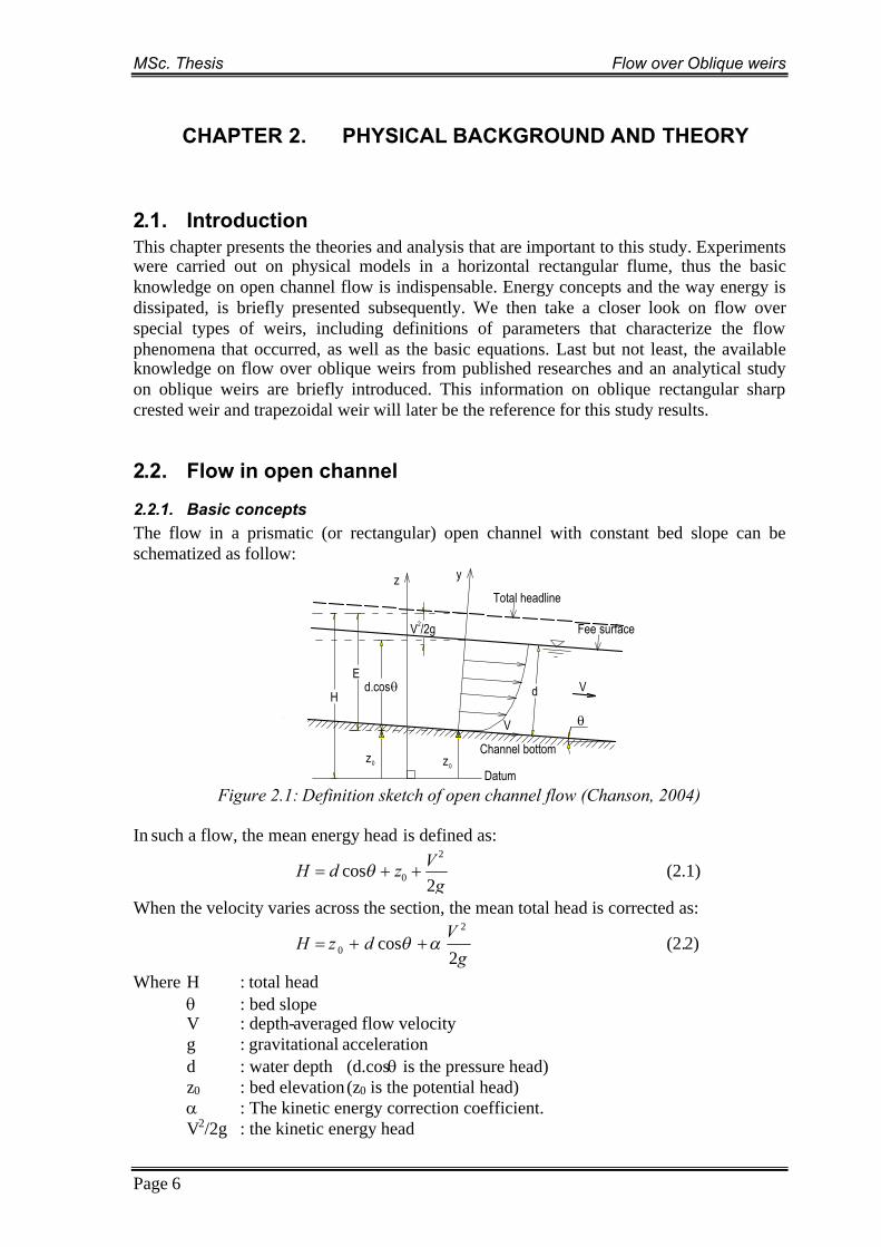
2.2.1. Basic conceptsThe flow in a prismatic (or rectangular) open channel with constant bed slope can beschematized as follow:
V
H
Ed.cos
d
Channel bottom
Datumz0 0z
V /2g2
z y
Total headline
V
Fee surface
Figure 2.1: Definition sketch of open channel flow (Chanson, 2004)
In such a flow, the mean energy head is defined as:2
0cos2VH d z
g (2.1)
When the velocity varies across the section, the mean total head is corrected as:
gV
dzH2
cos2
0 (2.2)
Where H : total head : bed slopeV : depth-averaged flow velocityg : gravitational accelerationd : water depth (d.cosis the pressure head)z0 : bed elevation(z0 is the potential head) : The kinetic energy correction coefficient.V2/2g : the kinetic energy head

MSc. Thesis Flow over Oblique weirs
Page 7
The Bernoulli equation describing energy conservation along a streamline is:
constg
VdzH 2
cos2
0 (2.3)
The specific energy:The specific energy is the flow energy with regard to the channel bed as datum. It reads:
gV
zHE2
2
0 (2.4)
If we consider a rectangular channel of width B and horizontal bottom, the specific energycan be written in terms of flow rate per unit width, q = Q/B, as:
2
2
2gyqyE (2.5)
In which Q is the total discharge, y is the flow depth.
Flow states:For the channel in our experiment (constant width), with a given discharge Q, the flow rateq remains constant along the flow meanwhile the depth y varies. The so called specificenergy diagram, for E = E(y) with a fixed value of q is shown in the following figure.
For a given value of flow rate and specific energy,the flow may have two possible depths, which aretermed alternate depths. These two depths, whichare presented on two branches of the E = E(y)curve, are characteristics of two different regimes ofthe flow, namely super-critical flow (at small depthy1) and sub-critical flow (at larger depth y2). Point Cin the diagram represents the transition state of theflow between the two regimes - the critical state. Itcan be defined as the state at which the specificenergy is minimum for a given flow rate.
Figure 2.2: The specific energy diagram
Critical state of the flow:By differentiation to find the minimum of the specific energy (Emin) from equation (2.4),we obtain the value of the critical depth. Then substituting this value of yc back into theequation we obtain Emin.
3
2
gq
yc (2.6) cyE23
min (2.7)
This means at the critical state of flow, the velocity head is equal to half the hydraulicdepth. The critical velocity is:
cc
c ygyq
V (2.8) 1yg
V, this dimensionless parameter is
defined as the Froude number.
Froude number:The Froude number is important in open channel flows. It is defined as the ratio of the lowvelocity (V) to the wave velocity (c).

MSc. Thesis Flow over Oblique weirs
Page 8
ygV
cVFr
(2.9)
The flow state is super critical when Fr > 1 and sub critical when Fr <1. The characteristicof the flow strongly depends on which state it is, and may be completely different for supercritical flow than for sub critical flow.
When Fr > 1, i.e. V < c, the flow velocity is smaller than the wave velocity, its fluidmoving in a tranquil manner, the waves or disturbances at downstream can propagateupstream. Thus the upstream locations are in hydraulic communication with thedownstream locations. On the other hand, when Fr > 1, i.e. V > c, the stream is movingrapidly so that the flow velocity is greater than the wave speed. In this case, nocommunication between upstream locations and downstream locations is possible(Munson, 2003); the flow is not influenced by the downstream water depth.
2.2.2. Resistance in the flow
Energy loss in open channel flow is due to hydraulic resistance, including wall roughness,viscosity, cross-sectional shape, boundary non-uniformity, the unsteadiness of the flow,and turbulences. General speaking, the resistances can be divided into two distinction typesso called surface resistance and form resistance. The surface resistance is caused by theroughness of the bottom, the side walls and the weir surface. The form resistance is causedby the local acceleration, deceleration and stagnancy of the flow. Normally the formresistance is much larger than the surface resistance, thus the surface resistance can oftenbe neglected (Bloemberg, 2001).
In an open channel flow, energy is continually dissipated, whether the flow is laminar (atlow Reynolds number, Re < 1000) or turbulent (Re >1000), eventually the energy isconverted into heat due to the effect of viscosity.
There are several formulas to calculate the energy loss in an open channel flow without aweir. The most frequently used formulas relating the mean flow velocity to resistancecoefficient are:
V C RS (Chezy) (2.10)2/13/249.1
SRn
V (Manning) (2.11)
fgRS
V8
(Darcy – Weisbach) (2.12)
WhereC, n, f : the Chezy, Manning and Weisbach resistance coefficients respectively.R : the hydraulic radius of the flow, R = A/P is the ratio between the crosssectional area and the wet perimeter of the flow.S : the flow resistance slope (the energy slope or friction slope)
Here in this study, because of some objective difficulty, the loss in the water depth of theflow due to resistances cannot be measured. Hence the result from an earlier research ofUijttewaal and Booij (2001) on the same flume and typical flow conditions will be used.For both low upstream water depth (42mm) and high upstream water depth (67mm), theloss over five meter distance approximates 1mm.

MSc. Thesis Flow over Oblique weirs
Page 9
The bottom shear stress:Starting from the momentum balance for a control volume in a schematized straight openchannel flow, we come up with a general expression for the shear stress at a verticalposition below the free surface:
izhg (2.13)where i is the bottom slope and h is the flow depth. At the bottom of the channel, z = 0, thebottom shear stress then is:
2
01 . .2 fg h i c u (2.14)
thus define a friction coefficient.
2.2.3. Turbulence and energy lossTurbulent is one of the most prominent properties of the flow because most of the flowsencountered in nature and technical installations are turbulent flows. It is the manner offlow in which various flow quantities show a random variation with time and space. Thetwo most important types of turbulence are free turbulence and wall turbulence. Turbulenceis capable of transfer energy of the flow from the mean motion to the turbulent fluctuations.Those fluctuations will then induce turbulent shear stresses, and energy will eventually bedissipated into heat via the viscosity. (Uijttewaal, 2006)
Reynolds number:Turbulence will appear in flows with high Reynolds number (Re > 1000) with the presenceof a velocity gradient. In the experiments of this study, surface resistance and formresistance were present due to the bottom friction, wall friction, and the presence of a weirin the flow. The flow in these experiments was completely turbulent due to a highReynolds number, Re always higher than 2104.
The Reynolds number by definition is:
LU .Re (2.15)
Where U : the characteristic velocity differenceL : characteristic length : kinematics viscosity,=/ : dynamic viscosity : mass density of the fluid (water).
Energy dissipation:There are two main ways for the dissipation of energy in the flow, one is the viscousdissipation induced by the mean motion, and the other is the dissipation via the turbulentmotion. By considering the energy equations of the flow, we can see that the loss of energyfrom the mean motion is dominated by turbulence, and the work done by the Reynoldsstresses is much bigger than the direct dissipation due to viscous. Beside, for a flow at highReynolds number the turbulent shear stresses are generally much larger than the viscousshear stresses. That means the dissipation by work done against turbulent shear stressesalso has a much larger contribution to the energy loss in the flow (Uijttewaal, 2006).

MSc. Thesis Flow over Oblique weirs
Page 10
2.3. Flow over plain weirs
2.3.1. IntroductionThis paragraph deals with the question of how the flow over a weir is described andcalculated. First the flow over a weir will be classified in to different regimes for an easierinterpretation. Then different discharge formulas for those flow regimes will be introducedfor different weir geometries and flow regimes. Lastly, the equations to evaluate the energyloss will be presented.
The figure below provides a typical view of the flow over a weir. It is followed by theconvention of the relevant flow and geometrical parameters.
i=0
Figure 2.4: The convention of parametersNotation explanation:
H : energy heighth : the water depth with relative to (w.r.t.) the weir crestd : water depth w.r.t the channel bottomm : weir slopeLw : weir crest length (in the direction of the flow)aw : weir heightH : the energy lossQ : total dischargei : bottom slope
Subscripts: 0: upstream; 1: above the weir crest; 2: downstream.
2.3.2. Flow regimesThe classification of flow regimes is really necessary and helpful for the experimentprocess. An early classification by Escande (1939) divides the flow into four types.Although his classification refers to the cylindrical crested weir but it can be equallyapplied to all other overflow structures. Recently a study by Fritz and Hager (1998) hasstrengthened this classification by extending it with a trapezoidal weir with the downstreamslope of 1:2.
Depending on the downstream water depth, the flow regimes can be divided into four maintypes (Escande, 1939). In the order of raising downstream water depth, they are:
- (A) Hydraulic jump: with a clear bore (roller) located at or downstream of the weirstructure. In this case, the flow is not influenced by the downstream water depth.
- (B) Plunging flow: with the main stream following the downstream slope of theweir and with a clear surface roller. The flow is almost independent from thedownstream water depth.
- (C) Surface wave flow: with the main stream following the free and wavy surfaceand a recirculation zone near the bottom.

MSc. Thesis Flow over Oblique weirs
Page 11
- (D) Surface jet flow: the flow depth is larger; the surface is nearly horizontal andsmooth. The flow strongly depends on the downstream water depth.
(A) Hydraulic jump (B) plunging flow
(C) Surface wave flow (D) surface jet flowFigure 2.5: Four main types of flow
For the sake of simplicity, the flow is divided in to three regimes. According to Kolkman(1989), they are:
(1) Free flow: the flow is entirely independent of the downstream water depth. Aroller can be observed. (A combination of types A and B)
(2) Submerged flow: the flow is influenced by the downstream water depth. Theflow surface is nearly horizontal. (Type D)
(3) Transition regime: analogous to type C. It is also called the Undulated flow.
As we will discuss later, the transition flow regime also has the clearest backwardmovement behind weir, the so called recirculation, in comparison with the two other flowregimes. In other words, the size of the recirculation zone in the case of transition stateflow has the biggest size.
2.3.3. Weir geometrySharp crested weir:The weir is termed as sharp-crested if thelength of the weir in the direction of flow (L)is such that H/L >15 (Bos, 1976). [In practice,the crest length of the sharp-crested weir isusually less than 2.0 mm (French, 1985),requiring H to be > 30mm].
Fig.2.6: Sharp-crested weir geometryBroad crested weir:By definition, a broad-crested weir is astructure with a horizontal crest above whichthe fluid pressure may be consideredhydrostatic (Fig.2.5). The following inequalitymust be satisfied for such weirs (Bos, 1976):
5.008.0 1 wL
H
Fig.2.7: Broad-crested weir geometryDike form weir (trapezoidal weir):This type of weir is chosen to be investigated further than the two types above because ofthe problems related to summer dikes and other obstacles in the flood plain, as described
H
.
.
Nappe
Weir plate
Q
Drawn down
a w
d2aw
d0
L
h0
V0Weir block
h1V1
w

MSc. Thesis Flow over Oblique weirs
Page 12
earlier. The upstream and downstream slopes of the weir are chosen as 1:4 according to theDutch norm for dike design.
2.3.4. Energy loss with the present of weirThe energy loss in the flow over a weir is due to incomplete conversion of kinetic energyinto potential energy (Ref.1). Upstream of the weir, in the acceleration area, part of thepotential energy of the flow is converted into its kinetic energy. While the water is flowing,it continuously losing energy against surface resistance, but this loss is negligible smallwith regard to the loss in form resistance. The mechanism of form resistance here is: part ofthe kinetic energy of the flow is converted into energy of vortices of all scales, andturbulent fluctuations; then this supply of energy will eventually be dissipated into heat viathe viscosity.
The following figure illustrates different zones in the flow over a weir according toHoffmans (1992).
Figure 2.8: Definition of flow zones
As mentioned earlier, the energy loss of the flow over a weir, or form resistance, is muchlarger than the loss in surface resistance. In the existing theories, discharge relations areoften used to express the energy loss. The discharge value can be used to calculate thewater depth and velocity of the flow. Knowing the water depth and velocity of the flow upand downstream of the weir, the decrease in energy height can be calculated. The dischargeitself strongly depends on the downstream water level (depends on which flow regimes)and the weir geometry. Later in chapter 4 of this report, the discharge coefficient and itsrelations with other flow parameters will be the subject of investigation.
2.3.5. Discharge coefficient - Cd and Cdv
Because of the complex nature of the flow, it is impossible to obtain a clear expression forthe flow rate as a function of other relevant parameters. An experimentally determinedcorrection factor Cd was then used to account for the various real world effects not includedin the simplified analysis to get the actual flow rate as a function of the water headupstream.
We denote Cd as the discharge coefficient for submerged flow and Cdv as the dischargecoefficient for the free flow (Cd perfect). For the physical meaning, Cdv represents theinfluence of the weir geometry on the maximum discharge over weir, meanwhile Cdrepresents the combined influences of the weir geometry and the downstream water headon the discharge over weir.
The discharge coefficient in case of a free flow (or so called the perfect weir) Cdv isindependent of the downstream water level and depends on the upstream flow conditiononly. It is given by:

MSc. Thesis Flow over Oblique weirs
Page 13
00 32
.32
gHHB
QCdv (2.22)
For an imperfect weir, the discharge coefficient depends on the downstream flow waterhead, it decreases when the water head increases. Also there is no explicit relation betweendischarge and water head for the case of submerged flow and flow in transition state. Adischarge reduction coefficient C* is introduced to account for the reduction in thedischarge coefficient of the perfect weir.
dv
d
CCC * (2.23)
C* itself is a function of the weir geometry andsubmergence (S=H2/H0). There are many formulas todetermine C*, for example the analytical formulaapplies for sharp weir by Seida and Quarashi(Kolkman, 1989), the semi-empirical relation byVillemonte (Kolkman, 1989), Varshney and Mohanty(Kolkman, 1989). Nowadays, the most suitable andwidely used formula is an entirely empirical formulaby Villemonte (1947):
PSC 1* (2.24)Figure 2.9: The relation between C* and S, p=525.
The fit parameter p depends on the geometry and configuration of the weir. The abovefigure illustrates the relation between C* and S for different values of p.
The study of Bloemberg (2001) has given some relations of Cd and Cdv with otherparameters, i.e. Cdv decrease with either increase the weir downstream slope m2, or increasethe relative weir height (a/H1), or decrease the relative weir length (H1/Lw). (Ref.1). Afunction for Cdv is given by Hager (1998):
55.0sin06.043.0
31
32
dvC(2.25)
Where wLHH
1
1 is the relative weir crest length. When 0.1<<0.3, the weir is long
crested; when 0.2<<0.6, the weir is short crested; and when =1, the weir is sharp crested.
Some important relations of Cd with other parameters were also mentioned by Bloemberg(2001). They are: Cd increases with either decreasing the downstream slope (gentler), ordecreasing the relative energy height (H1/Lw), or increasing the angle of the incoming flowwith the weir. Later in this study we will see that the last comment on the relation betweenthe oblique angle and Cd is not completely right.
2.3.6. Discharge formulas
As discussed above, the discharge formula can be use to calculate the water depth andvelocity of the flow. Following are some well known formulas that are often used tocalculate the discharge for some types of weir.
0 0.2 0.4 0.6 0.8 10
0.2
0.4
0.6
0.8
1
S=H2/H
0C
*
p=5
p=25

MSc. Thesis Flow over Oblique weirs
Page 14
Sharp crested weirThe energy conservation equation for a weir is:
23
..232
HBgQ (2.26)
Numerous approximations have been used to obtain the above equation, namely the neglectof the viscous effects, turbulence, non-uniform velocity distributions, and centripetalaccelerations in the derivation of this discharge equation. To obtain the actual flow rate as afunction of weir head, an experimentally determined correction factor (Cws) must be used.The final form, suggested by Kindsvater and Carter (1957) is:
23
232
. eews hgBCQ (2.27)
where Be : the effective width of the weirhe : the effective water headCws : the (dimensionless) effective discharge coefficient.
Cws is a function of Reynold number (viscous effects), Weber number (surface tensioneffects), and H/Pw (geometry parameter) (where aw is the height of the weir). In mostpractical situation, the Reynold and Weber number effects are negligible, and the followingformula can be used (Rehbock, 1929):
wws a
HC 075.0611.0 (2.28)
Broad crested weirThe equation for discharge is again (2.26). To account for various real world effects notincluded in the simplified analysis, again an empirical weir coefficient, Cwb, is used(Munson, 2002):
23
32
32
. HgBCQ wb (2.29)
The broad-crested weir coefficient Cwb can be obtained from the formula (Munson, 2002):
w
wb
aH
C
1
65.0(2.30)
The broad-crested weir is considerably more sensitive to geometric parameters incomparison with the sharp-crested weir. Those parameters include for example the surfaceroughness of the crest and the shape of the leading-edge nose (sharp or rounded).
Submerged flowFor the submerged flow, the submerged coefficient Ks should be introduced into equation2.27 and 2.29 to produce submerged discharge Qs. The general formula is:
QKQ ss . (2.31)
Since 2/303
232. HgBCQ ds and 2/3
032
32. HgBCQ vd
dv
ds C
CK (2.32)
Thus KS can be interpreted as the discharge reduction coefficient C* in the formula ofVillemonte. They can be compared to each other for the same flow condition.

MSc. Thesis Flow over Oblique weirs
Page 15
Brater and King (1976) suggested the following form for the experimental coefficient Ks(for a plain weir):
385.0
23
0
21
HH
K s (2.33)
Wu and Rajaratnum (1996) also suggest a formula (for plain weir):
0
21
0
2 sin.331.1162.11HH
HH
K s (2.34)
Where H0 and H2 is the upstream head and downstream head respectively. Here thedownstream condition starts playing a role.
2.3.7. Energy balance and Momentum balance
The main mechanisms governing the flow over a weir are gravity and inertia; other effectslike viscous and surface tension are of secondary importance. As mentioned earlier, for asteady flow, the Bernoulli equation, which is an energy equation, can always be appliedtaking into account certain portion of energy losses. Providing proper allowance for allforces acting, the momentum equation always holds true as well.
Generally speaking, in the analysis of a flow, the energy and momentum equations play acomplementary role for each other. Usually the information which is not supplied by oneequation is provided by the other. Together with the continuity equation, they provided theanalytical means to assess the energy loss in the flow over a weir.
Energy balance:Upstream of the weir, the energy is usually assumed to be constant. If we consider a reachof only two meters from weir center, usually the loss due to bed friction is small, and theconstriction of the flow when it reaches the weir causes almost no loss. The Bernoulliequation for two cross sections one upstream and one above the weir, with the level of theweir crest as the reference level, reads:
1
21
10
20
0 22p
gu
hpg
uh (2.35)
Usually the atmospheric pressure is constant in the laboratory, p0 = p1. The upstream totalhead then can be written as a function of flow condition above the weir:
1
21
1
21
10 22h
Frh
gu
hH (2.36)
21
21
10
FrhH (2.37)
Downstream from the weir, the energy is no longer conserved. Energy loss (and also headloss) is sometimes significant, especially for free flow over weir. The widening anddeceleration of flow and the turbulence downstream of the weir account for the main partof losses. A parameter representing these losses is the discharge coefficient (Cd), given inequation 2.22. Substitute H0 into this equation leads to a relation of the dischargecoefficient and the flow condition (Fr1 is unique for each flow state):

MSc. Thesis Flow over Oblique weirs
Page 16
2/3211
12/32
12/31
2/3
11
2/30
233
22
32
.
.32
.32 Frgh
u
Frhg
hu
HgB
QCdv
2/32
1
1
2
33
Fr
FrCdv
(2.38)
The above relation can be used for imperfect weir, when the flow on top of the weir is sub-critical, as well. It will be used to check with measurement data later. The following figureillustrates this relation.
0 0.2 0.4 0.6 0.8 10
0.2
0.4
0.6
0.8
1
Fr1 (m)
Cd
Cd
~ Fr1
Figure 2.10: Cd as a function of Fr1.It should be note that here the energy conservation is assumed and Cdv is only governed bythe conditions above the weir crest.
Momentum balance:Downstream of the weir, the momentum equation is of great importance when the energyequation breaks down in the presence of unknown energy losses. With complement resultsfrom the momentum equation, the energy loss can be estimated.
The submergence is an indicator for the water head loss over the weir, and the Froudenumber above the weir is an important dimensionless parameter, which determines theflow regimes. The link between these two parameters is thus of interest. With theassumption of momentum conservation in the downstream part of the weir, this relation canbe found by an iterative process.
The momentum balance equation for the downstream part of the weir reads:
222
221
21
21 2
1)(
21
hughhuahg w (2.39)
Combine with the simplified form of the continuity equation:2211 huhu (2.40)
Equation 2.39 can be rewritten as follows:
022121 2
212
222
22
122
312
2
FrhFr
ha
hha
hh
(2.41)
Knowing the value of h2, h1 can be found as a root of the above polynomial. Otherdependent parameters can be calculated as well. The relation between S (S=H2/H0 is the

MSc. Thesis Flow over Oblique weirs
Page 17
submergence) and Fr1 can be found by repeating the above process for a certain range ofh2. It can be illustrated in figure 2.11.
0 0.2 0.4 0.6 0.8 1 1.20
0.2
0.4
0.6
0.8
1
Fr1
SQ = 20l/sQ = 30l/sQ = 40l/s
Figure 2.11: The submergence as a function of Fr1 .
2.4. Flow over oblique weirAs mentioned earlier, not many studies on oblique weirs have been published. In thefollowing, studies of Borghei, De Vries and Wols will be briefly introduced. And then thetheoretical analysis of the flow over an oblique weir will be presented. The angle betweenthe longitudinal axis of the weir and the direction normal to the flow (angle in the figurebelow) is referred to as “oblique angle” from now on.
2.4.1. Oblique sharp crested weir
The study of Borghei et al (2003) discusses theirexperimental result with existing dischargeformulas, particularly for rectangular sharp-crestedweirs with different upstream and downstream beds.
Figure 2.12: Plan view of an oblique weir.
The general formula for flow measurement with a small amendment (using the effectiveweir length L instead of channel width B) can be used:
23
0..232
. HLgCQ d (2.42)
For a plan and full width weir, Cd can be calculated by equation (2.28). The general form is
wd a
HbaC 0
(2.43)The results of the research show that for a plain sharpcrested weir, Cd is only a function of H0/aw if the waterhead is large enough to minimize any surface tensioneffects. Therefore, it is possible to find the values of aand b in the above equation for each different obliqueangle using the experimental results and determine ifthere is only one coefficient of discharge relationshipfor all angles.
BL
Flow
Oblique weir
Q
Figure 2.13: Free flow
H
aw
0Q

MSc. Thesis Flow over Oblique weirs
Page 18
For free flow, it shows a trend of decreasing Cd as the ratio H0/aw increases. That means theoblique weir should be used for low values of H0/aw. The results also showed thatincreasing the ratio H0/aw will decrease the convergence capacity. Another important resultis that, for the same discharge, using an oblique weir instead of a plain weir will decreasethe water head noticeably.
For a rectangular sharp-crested weir, the standard equation of Cd is approximated as:
wd a
HLB
LB
C )663.1229.2121.0701.0 (2.44)
Where (B/L) = cos; is the oblique angle.
For submerged flow (figure 2.14), Borgheisuggested the following formula for submergecoefficient:
23
0
2
HH
dcK s (2.45)
Figure 2.14: Submerged flowWhere c and d are coefficients and can be found in plots in the report of Borghei, (2003).And the general form of Ks is:
23
0
2479.0161.0985.0008.0
HH
BL
BLK s (2.46)
It should be note that the above formulas are only based on observations of small H0/Pwconditions.
2.4.2. Oblique trapezoidal weirAnother published research on oblique weirs is the report of De Vries, TU Delft 1959. Hehad performed a large number of experiments to examine the loss of the flow over dike-form weirs under different oblique angles and flow conditions.
He considered the two equations to calculate thecapacity of the flow over a plain weir (2.47) andflow over an oblique one (2.48):
gHBmQ s 32
32... 2/3
(2.47)
gHLmQ k 32
32... 2/3
(2.48)
Figure 2.15: De Vries experimentWhere Bs is the channel width and Bk is the effective width of the weir.Because of cos.LB (2.49)Then a relation for the two discharge coefficients can be deduced:
cosk
s
mm (2.50)
Finally he introduced a reduction factor p to account for the effect of the length of the weir,the submerged flow condition, the limited width, and the energy height which should becalculated with the velocity component perpendicular to the weir only:
a
HHd
w
0
Q
MSc. Thesis Flow over Oblique weirs
Page 19
cos. 0k
s
mpm (2.51)
p then can be interpreted as the reduction factor of the discharge coefficient due to theobliqueness of the flow concerning a restricted width of the channel:
0k
k
m
mp (2.52)
De Vries has performed several experiments on physical scale model with the geometricalscaling of 25. Some parameters including the channel width (Bs), the specific discharge (q),the weir height (aw), and specially the oblique angle (), were altered; whereas the crestwidth (Lw) and the slopes (m) of weir were kept constant Lw = 3m and m = 1:4.
Some overall conclusions from his research are:- The reduction factor p decreases when increasing the oblique angle .- The reduction factor p decreases when the submergence (S = H2/H0) increases.- With a given value of p, the variation of B causes no significant changes in the flow
width.- When the submergence S reaches the limit of 1, p converges to the value of cos.
De Vries also further investigated the relation between the discharge coefficient m withother parameters, specially the submergence S, for different oblique angle 30, 45 and 600
and produced graphs which are very interesting to be compared with results from this study(Flow over oblique weirs).
2.4.3. Numerical simulations on oblique weirs
The numerical simulations from Wols (2005) were performed with the k-turbulencemodel and the non-hydrostatic finite elements model FINLAB. He has done extensivesimulations on different types of weirs, and tried to reproduce some of the experiments onphysical scale models. Those include perpendicular and oblique weirs, sharp and longcrested weirs, triangular weir, trapezoidal weirs, and rectangular weirs. The results ofsimulations were then compared to the results of experiments. Thanks to the competence ofthe computer models, he could run more simulations than physical model tests, investigatethe three dimensional structure of the modeled flows, and thus gained further informationon flow over different types of weirs.
For perpendicular weirs, the discharge coefficients can be obtained on the basis of theupstream flow energy conservation as long as the streamline is horizontal. For the sharpweirs and in free flow (perfect weir), the streamlines could no longer be considered ashorizontal, the non-hydrostatic impact was strong and the discharge coefficients showedvalues larger than one. Energy loss can be obtained on the basis of downstream flowmomentum balance, and was described by the relation between the Froude number abovethe weir and the ratio H2/H0.
The simulations for flow over oblique weirs showed similarities with the analytical analysisin the case of a dike form and sharp crested weirs. The direction of the flow streamlinesand the energy loss depends on the Froude number above and upstream of the weir. Theflow over an oblique weir can be treated as flow over a plan weir if we consider thevelocity component normal to the weir. The velocity component parallel to the weir ismore or less constant in the flow field. This analysis gave good result for discharge
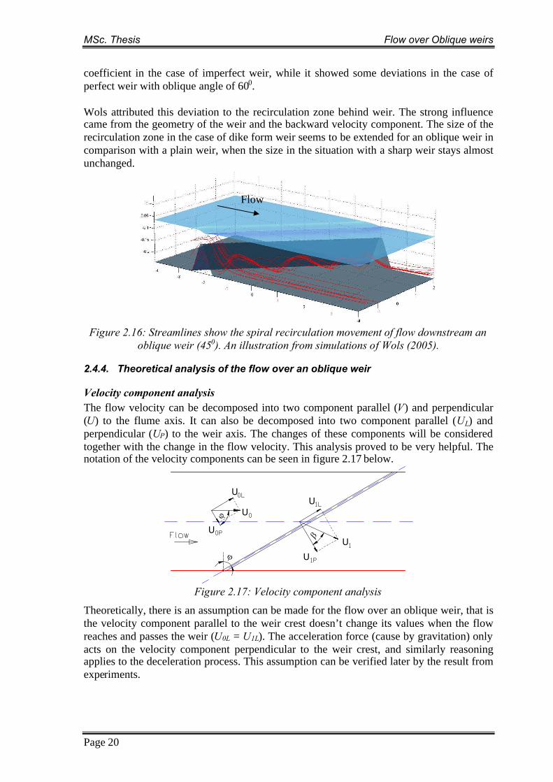
MSc. Thesis Flow over Oblique weirs
Page 20
coefficient in the case of imperfect weir, while it showed some deviations in the case ofperfect weir with oblique angle of 600.
Wols attributed this deviation to the recirculation zone behind weir. The strong influencecame from the geometry of the weir and the backward velocity component. The size of therecirculation zone in the case of dike form weir seems to be extended for an oblique weir incomparison with a plain weir, when the size in the situation with a sharp weir stays almostunchanged.
Figure 2.16: Streamlines show the spiral recirculation movement of flow downstream anoblique weir (450). An illustration from simulations of Wols (2005).
2.4.4. Theoretical analysis of the flow over an oblique weir
Velocity component analysisThe flow velocity can be decomposed into two component parallel (V) and perpendicular(U) to the flume axis. It can also be decomposed into two component parallel (UL) andperpendicular (UP) to the weir axis. The changes of these components will be consideredtogether with the change in the flow velocity. This analysis proved to be very helpful. Thenotation of the velocity components can be seen in figure 2.17 below.
U
U
UU
U
U
Figure 2.17: Velocity component analysis
Theoretically, there is an assumption can be made for the flow over an oblique weir, that isthe velocity component parallel to the weir crest doesn’t change its values when the flowreaches and passes the weir (U0L = U1L). The acceleration force (cause by gravitation) onlyacts on the velocity component perpendicular to the weir crest, and similarly reasoningapplies to the deceleration process. This assumption can be verified later by the result fromexperiments.
Flow

MSc. Thesis Flow over Oblique weirs
Page 21
Flow direction and flow condition above an oblique weirThe oblique angle of the flow is understood to be the deviation angle of the flow streamlinefrom the normal direction to the weir. It is called (see figure 2.17). For a plain weir (=00), the flow streamlines are perpendicular to the weir crest, thus = 0 (this also impliesthat U1L = 0). For an oblique weir (< 900), the value of can be predicted using theenergy conservation and continuity assumptions of the flow.
Figure 2.18: Upstream energy balance
With weir crest as the reference level, the energy balance equation applied to the upstreampart of the weir reads:
gu
hg
uh
22
21
1
20
0 (2.53)
The continuity equation always holds true for the flow: LhuLahu PwP .. 1100 (2.54)
where L is the length of the oblique weir, L = B/cos(B is the channel width).By decomposing each of the velocities into two components:
20
20
20 LP uuu ; 2
12
12
1 LP uuu (2.54)
An important assumption is made here: the velocity component parallel to the weir crest isconstant everywhere in the area of investigation, i.e. u0L = u1L. This assumption will becorroborated later in chapter 5.
And together with the continuity equation, equation 2.53 becomes:
gu
hg
uh PP
22
21
1
20
0
0.22
1110
31
130
huu
gu
haug PP
PwP (2.55)
Given the value of h1, the value of u1P can be calculated, and u0P can be found as a root ofthe above polynomial. Other upstream parameters can be calculated as follow:
cos0
0Pu
u ; wauB
Qh
00 .
(2.56)
Then u1 can be calculated from equation 2.53. Finally the oblique angle of the flowstreamlines above the weir is found:
1
1arccosuu P (2.57)
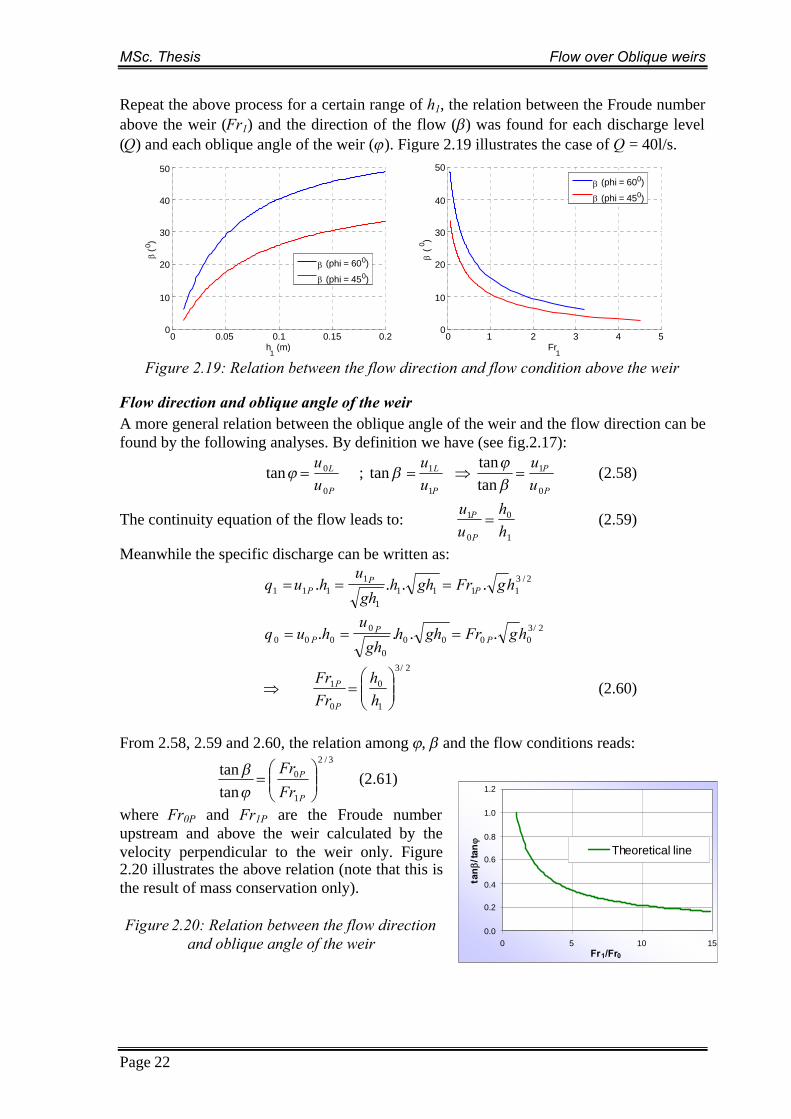
MSc. Thesis Flow over Oblique weirs
Page 22
Repeat the above process for a certain range of h1, the relation between the Froude numberabove the weir (Fr1) and the direction of the flow () was found for each discharge level(Q) and each oblique angle of the weir (). Figure 2.19 illustrates the case of Q = 40l/s.
0 0.05 0.1 0.15 0.20
10
20
30
40
50
h1
(m)
(0 )
(phi = 600)
(phi = 450)
0 1 2 3 4 50
10
20
30
40
50
Fr1
(0 )
(phi = 600)
(phi = 450)
Figure 2.19: Relation between the flow direction and flow condition above the weir
Flow direction and oblique angle of the weirA more general relation between the oblique angle of the weir and the flow direction can befound by the following analyses. By definition we have (see fig.2.17):
P
L
uu
0
0tan ;P
L
uu
1
1tan P
P
uu
0
1
tantan
(2.58)
The continuity equation of the flow leads to:1
0
0
1
hh
uu
P
P (2.59)
Meanwhile the specific discharge can be written as:2/3
11111
1111 .... hgFrghh
gh
uhuq P
PP
2/30000
0
0000 .... hgFrghh
gh
uhuq P
PP
2/3
1
0
0
1
hh
FrFr
P
P (2.60)
From 2.58, 2.59 and 2.60, the relation among , and the flow conditions reads:3/2
1
0
tantan
P
P
FrFr
(2.61)
where Fr0P and Fr1P are the Froude numberupstream and above the weir calculated by thevelocity perpendicular to the weir only. Figure2.20 illustrates the above relation (note that this isthe result of mass conservation only).
Figure 2.20: Relation between the flow directionand oblique angle of the weir
0.0
0.2
0.4
0.6
0.8
1.0
1.2
0 5 10 15Fr1/Fr0
tan
b/ta
nj
Theoretical line

MSc. Thesis Flow over Oblique weirs
Page 23
ConclusionThe results and conclusions from above presented available studies on oblique weirs willbe brought into comparison with new results from this study in order to see similarities anddifferences. Taken into account the differences caused by different types of oblique weirsand experimental conditions, similarities can be found. Meanwhile, the theory analysis onoblique weirs, which are based on fluid continuity, momentum conservation and energyconservation, are important for the anticipation and interpretation of experiment data. Thedecomposition of a velocity vector is an important step in order to study the flow over anoblique weir. Understanding of intrinsic properties of flow over an oblique weir is theultimate goal.

MSc. Thesis Flow over Oblique weirs
Page 24
CHAPTER 3. SET-UP AND IMPLEMENTATION OFEXPERIMENTS
3.1. IntroductionThe main purpose of these experiments is to determine the loss in water head, energy headover oblique weirs with different configurations. Besides, they also aim at a qualitativedescription of other complex phenomena that happen near a weir in the flow. To fulfillthose purposes, the experimental setup should include the choice of parameters toinvestigate, the design of the physical models, and the elaboration of experiments. Thoseprocedures will be treated in this chapter.
Experiments were carried out on physicalscale models in the the Fluid MechanicsLaboratory of Technical University ofDelft. Different weir’s geometries includesharp crested weir, broad crested weir, anddike-form weir were tested. The dike-formweir is further investigated with differentoblique angles to the flow direction: 0(plain weir), 45 and 60 degrees.
Figure 3.1: The experiment site in theLaboratory.
The flow over an oblique weir showsasymmetrical behavior across the channel width. To investigate intrinsic properties of theflow in these cases we should avoid the areas where the flow is disturbed too much by theside wall effect (the effect of a solid boundary). That is the main reason for conductingthese experiments in a shallow flume with the flume width much larger than the flow depth(in the order of ten times). Hereafter the measurement elaboration, implementation and datainterpretation methods will be described.
3.2. Experimental parameters
3.2.1. Choosing experiment parametersThe first step to study this research is to determine which parameter (or factor) plays a rolein the flow over an oblique weir. The list should include the most important parameters thatdetermine the geometry, material properties and the external effects (including thehydraulic conditions). The main geometry parameters are the channel width (B), weirheight (aw), oblique angle (), and the weir crest length (Lw). The hydraulic parametersshould include the discharge (Q), flow depth (d), velocity (u), and the flow direction ().Main mechanisms governing the flow over a weir are gravity and inertia, thus thegravitational acceleration (g) and the fluid density () is also of importance. The materialproperties and viscosity play a lesser role and will not be considered explicitly here. Otherdependent hydraulic parameters (Re, Fr, S, q...) can be calculated from the main variables.

MSc. Thesis Flow over Oblique weirs
Page 25
The next step is to develop a meaningful and systematic way to perform experiments.During the research, basically an interested topic will be investigated by observing thephenomenon or the object parameter when changing one variable and holding othersconstant. More than one variable will be tested in this manner to get the data for theanalyses of a more complex phenomenon. Each of the above series of tests will helpcollecting data that can be visualized by charts and figures.
An effective and simple method is to work with non-dimensional combinations of variablesinstead of working with single parameters one by one. We can work with for example theFroude number (Fr), which is a combination of the flow depth, velocity and thegravitational acceleration. The dimensionless parameter Fr is very important for the flowwith a free surface. We can also consider the submergence (S), which is the ratio betweenthe downstream water head and the upstream water head; instead of consider many singleparameters involved. By using this approach we can significantly reduce the number ofanalyses and the results will be more general, universal and useful.
Main variables to be investigated and their range in this study are presented in thefollowing table:
Table 3.1: Experiment variables
Range of valuesVariables Dimension
Dike-form weirs Rectangular weirs
Discharge l/s 20, 25, 30, 35, 40 16, 20, 35
Water head cm 13 ÷ 18.5 13 ÷ 18.5
Downstream water head cm 8.5 ÷ 18 8.5 ÷ 18
Oblique angle degrees 0, 45, 60 45
Weir length cm 200, 283, 400 283
Weir height cm 10 10.4 10
Channel width cm 199 200 200
Number of tests - 15 x 5 x 3 8 x 5 + 5 x 5
3.2.2. Dimensional analysis, scaling and similitudeAn obvious goal of any experiments in general and these experiments in particular is tomake the result as widely applicable as possible. In a certain constriction of the laboratoryconditions, the experiments made on physical scale models should be able to result inempirical formulations, predict characteristics and behaviors of other similar systemsoutside the laboratory. To do this, the relation between the laboratory model and the realsystem must be established.
Physical interpretations can be given to dimensionless groups, which are also called thedimensionless products, and are frequently referred to as “pi terms” (). This interpretationproves to be very useful. The Froude number (Fr), physically presents the ratio of inertiaforce and gravitational force, was showed to be the most common and useful “pi term” foralmost all problems in experiments with the open channel flow. It will be used extensivelyin this study.
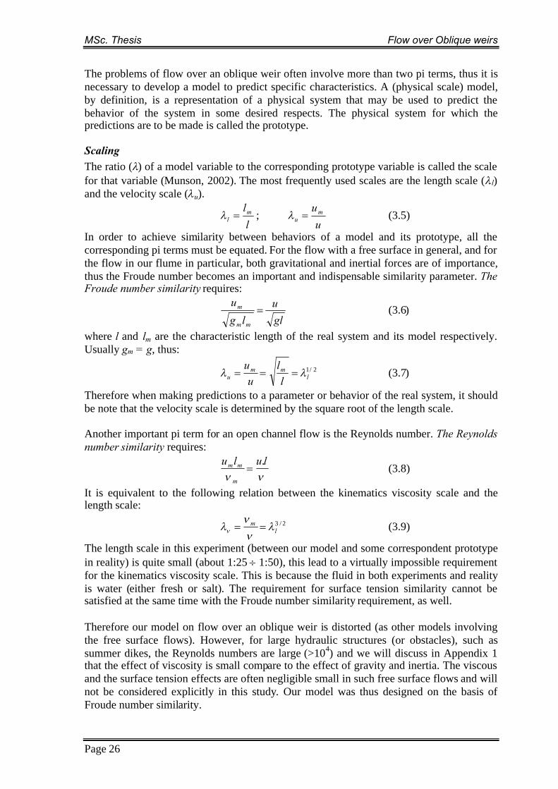
MSc. Thesis Flow over Oblique weirs
Page 26
The problems of flow over an oblique weir often involve more than two pi terms, thus it isnecessary to develop a model to predict specific characteristics. A (physical scale) model,by definition, is a representation of a physical system that may be used to predict thebehavior of the system in some desired respects. The physical system for which thepredictions are to be made is called the prototype.
ScalingThe ratio () of a model variable to the corresponding prototype variable is called the scalefor that variable (Munson, 2002). The most frequently used scales are the length scale (l)and the velocity scale (u).
llm
l ;u
umu (3.5)
In order to achieve similarity between behaviors of a model and its prototype, all thecorresponding pi terms must be equated. For the flow with a free surface in general, and forthe flow in our flume in particular, both gravitational and inertial forces are of importance,thus the Froude number becomes an important and indispensable similarity parameter. TheFroude number similarity requires:
glu
lg
u
mm
m (3.6)
where l and lm are the characteristic length of the real system and its model respectively.Usually gm = g, thus:
2/1l
mmu l
lu
u (3.7)
Therefore when making predictions to a parameter or behavior of the real system, it shouldbe note that the velocity scale is determined by the square root of the length scale.
Another important pi term for an open channel flow is the Reynolds number. The Reynoldsnumber similarity requires:
lulu
m
mm . (3.8)
It is equivalent to the following relation between the kinematics viscosity scale and thelength scale:
2/3l
m
(3.9)
The length scale in this experiment (between our model and some correspondent prototypein reality) is quite small (about 1:251:50), this lead to a virtually impossible requirementfor the kinematics viscosity scale. This is because the fluid in both experiments and realityis water (either fresh or salt). The requirement for surface tension similarity cannot besatisfied at the same time with the Froude number similarity requirement, as well.
Therefore our model on flow over an oblique weir is distorted (as other models involvingthe free surface flows). However, for large hydraulic structures (or obstacles), such assummer dikes, the Reynolds numbers are large (>104) and we will discuss in Appendix 1that the effect of viscosity is small compare to the effect of gravity and inertia. The viscousand the surface tension effects are often negligible small in such free surface flows and willnot be considered explicitly in this study. Our model was thus designed on the basis ofFroude number similarity.

MSc. Thesis Flow over Oblique weirs
Page 27
3.3. Design of weirsThe objects of the physical model are three weirs. They are made of composite, wood andconcrete, painted in white. General shape and dimensions are shown in the followingfigures:
3.3.1. Sharp crested weir:
Sharp crested weir
Flow
200cm
30cm
30cm
200cm
Figure 3.2: Sharp crested weir
3.3.2. Broad crested weir:
Flow
Broad crested weir
45°200cm
30cm
30cm
200cm40cm
40cm
Figure 3.3: Broad crested weir
3.3.3. Dike form weirs:
The upstream and downstream slopes of weir were chosen as 1:4, the ratio between theweir height and the crest width was chosen as 2. Those choices were made according to thetypical form of Dutch river dikes and in accordance with De Vries (1959). The obliqueangle is altered with 0, 45 and 600 .Following the case of 450 will be illustrated.
Figure 3.4: Dike-form weir
For a dike-form weir with a different oblique angle, the channel width and the weir crosssection (I-I) stay unchanged when the whole weir is rotated to the appropriate angle. Someextra pieces might be needed to extend the weir to the whole flume width.
1.2cm
1.2cm8.8cm
10cmFlow
Flow
40cm
10cm

MSc. Thesis Flow over Oblique weirs
Page 28
3.4. Major experimental equipments
3.4.1. Measurement siteThe experiments were conducted in a rectangular horizontal glass flume, 19.2 m long, 2 mwide, and 0.22m deep. In the middle area of the flume, the research object, which is awooden weir, is situated. The weirs in experiments had a general height of 10 cm and werepainted in white to serve the purpose of the PTV analysis.
The water for experiments was taken from and returned to the main circulation system inthe laboratory. The flow from a 250-mm conduit was discharged into a buffer basin andthen into the experimental flume. Its uniformity was improved by a double-layer filterscreen at the beginning of the flume to ensure that the approached flow to the weir at themiddle of the flume was uniform over the flume width and free of flow concentrations andsurface waves. At the end of the flume, the flow, occasionally together with polystyreneparticles from PTV measurements, flowed into a buffer basin through a filter. Here theparticles were trapped and collected later.
Water inlet
Area of interest
Oblique weir
CameraPlatform Flow
Particles supplier
Water outlet
End sill
Concrete blocks
Flow
Computer
Figure 3.5: Schematized plan view of the flume and its apparatus
Following are some of the main facilities that were used.
3.4.2. Point gaugesPoint gauges play an important role in this study. It wasused to draw the free surface profile of the flow,measure flow depth for energy loss and dischargecalculations, calibrate the discharge, and to depict theasymmetry of the flow over the flume width.
For those purposes, one common method was applied.First the elevation of the surface of the flow at a fixedpoint (in the plan view) was measured by the pointgauge, and then the elevation of the bottom at thatpoint. The later value was subtracted from the first oneto get the value of the flow depth.
There were two point gauges mounted on a moveablebeam in such a way that they can do the measurementacross the flume. The beam itself is mounted on theinstrument carriage, which can move along the flume
Figure 3.6: The instrument carriage.
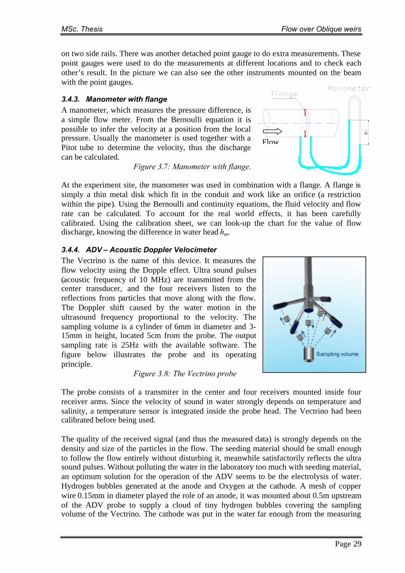
MSc. Thesis Flow over Oblique weirs
Page 29
on two side rails. There was another detached point gauge to do extra measurements. Thesepoint gauges were used to do the measurements at different locations and to check eachother’s result. In the picture we can also see the other instruments mounted on the beamwith the point gauges.
3.4.3. Manometer with flangeA manometer, which measures the pressure difference, isa simple flow meter. From the Bernoulli equation it ispossible to infer the velocity at a position from the localpressure. Usually the manometer is used together with aPitot tube to determine the velocity, thus the dischargecan be calculated.
Figure 3.7: Manometer with flange.
At the experiment site, the manometer was used in combination with a flange. A flange issimply a thin metal disk which fit in the conduit and work like an orifice (a restrictionwithin the pipe). Using the Bernoulli and continuity equations, the fluid velocity and flowrate can be calculated. To account for the real world effects, it has been carefullycalibrated. Using the calibration sheet, we can look-up the chart for the value of flowdischarge, knowing the difference in water head hm.
3.4.4. ADV – Acoustic Doppler VelocimeterThe Vectrino is the name of this device. It measures theflow velocity using the Dopple effect. Ultra sound pulses(acoustic frequency of 10 MHz) are transmitted from thecenter transducer, and the four receivers listen to thereflections from particles that move along with the flow.The Doppler shift caused by the water motion in theultrasound frequency proportional to the velocity. Thesampling volume is a cylinder of 6mm in diameter and 3-15mm in height, located 5cm from the probe. The outputsampling rate is 25Hz with the available software. Thefigure below illustrates the probe and its operatingprinciple.
Figure 3.8: The Vectrino probe
The probe consists of a transmiter in the center and four receivers mounted inside fourreceiver arms. Since the velocity of sound in water strongly depends on temperature andsalinity, a temperature sensor is integrated inside the probe head. The Vectrino had beencalibrated before being used.
The quality of the received signal (and thus the measured data) is strongly depends on thedensity and size of the particles in the flow. The seeding material should be small enoughto follow the flow entirely without disturbing it, meanwhile satisfactorily reflects the ultrasound pulses. Without polluting the water in the laboratory too much with seeding material,an optimum solution for the operation of the ADV seems to be the electrolysis of water.Hydrogen bubbles generated at the anode and Oxygen at the cathode. A mesh of copperwire 0.15mm in diameter played the role of an anode, it was mounted about 0.5m upstreamof the ADV probe to supply a cloud of tiny hydrogen bubbles covering the samplingvolume of the Vectrino. The cathode was put in the water far enough from the measuring
Flow

MSc. Thesis Flow over Oblique weirs
Page 30
point in order to avoid big oxygen bubbles to go to the sampling volume (these would givesharp decrease in the quality of signal, and produced wrong velocity data).
Figure 3.9: Typical arrangement of the ADV and the bubble generator.
The ADV probe needs some clearance in the water. Due to its size and shape, together withthe requirement of 5cm distance from the sampling volume to the probe, only a limited partof the flow can be measured by the ADV. Because of the flexibility of the ADV probe, itcan be mounted under different angles and directions. After having tried many solutions,the 450 rotated downward is chosen (see figure). This configuration gave an optimummeasuring range for the ADV; it can measure to the bottom of the flume, and rather closeto the free surface. The anode frame was also slanted to make the density of the bubbles tothe sampling volume better. In some special cases, for example to measure the velocity ontop of the weir, where the water layer is very thin, the ADV probe can be rotated 900 (lyinghorizontally).
Figure 3.10: The xyz coordinate of the instrument
The collected rough data need to be converted and processed in order to be useable later.Three velocity components on three orthogonal axis x, y and z of the probe would thenneed to be decomposed, rotated and recomposed to the orthogonal coordinate of the flume.These steps were done using Matlab. Since velocities are measured at a single point, onlytime series of the components of the velocity vector at that location can be obtained. Thisimplies that the Taylor hypothesis (or the frozen turbulence approximation) has to be usedin order to infer the spatial properties of the flow.
3.4.5. EMF – Electro Magnetic Flow meter
In these experiments, the EMF played a supplemental role to the ADV. It is capable ofmeasuring flow velocity reasonably close to the surface, where the ADV was not able tooperate. Moreover, in many cases the flow downstream of the weir is highly turbulent, thusthe supply of hydrogen bubbles is not fully adequate to the ADV probe. In those situations,the EMF needs to be used as a substitute.
The principle of an EMF is based on the induction law of Faraday, it follows that theinstantaneous velocity of a charged particle moving through a magnetic field isproportional to the measured voltage between two electrodes. The sampling volume is few

MSc. Thesis Flow over Oblique weirs
Page 31
cubic centimeters right underneath the probe with its electrodes. The advantage of an EMFis that it is easy to use and that it can measure two velocity components simultaneously(while the EMF is mounted vertically on the instrument beam, the vertical velocitycomponent is missed). Again the instrument needs to be calibrated and a calibration sheetis required. Before each measurement, it is necessary to check the zero-offset drift on themeasured signals.
The calibrated data from measurement needs to be scaled (and rotated) to the rightmagnitude of velocity. Using Matlab we can determine the time averaged velocitycomponents at the measurement point. Again the frozen vortex hypotheses of Taylor needto be applied to study the spatial structure of the flow.
3.4.6. Facilities for PTV analysisThe PTV analysis provided us with much more information than the single pointmeasurements. The flow with its properties was determined in many points simultaneously.
Here in this study, a one mega pixel CCD camera and the software Video Savant 4.0 wereused to capture flow images from a top view of the flume. The seeding used to visualize thesurface velocity field consist of floating black polystyrene particles with 3 mm diameter insize. They follow the flow satisfactory and reflect enough light to be captured by thecamera. To do so, one particle dispenser, which can cover the whole width of the flume,was placed upstream of the weir from an appropriate distance. If the distance is too close,the flow surface will be disturbed too much by the dispensed particles. If the distance is toofar, the particles will stick together while they are moving, thus generating unusable data orerrors for the PTV analysis. The dispenser was also equipped with a vibrator to provide abetter distribution of the particles.
The number of particles in an image of the flow is rather important for the processing step.They can contribute significantly to the time and quality of a PTV analyses, and to obtain agood signal peak in the cross-correlation of the PIV technique. A rule of thumb is 10 to 25particles images should be seen in each interrogation area (a concept coming from PIVanalysis; an interrogation area approximates 20cm x 20cm).
Figure 3.11: The flow seeded with black tracers.
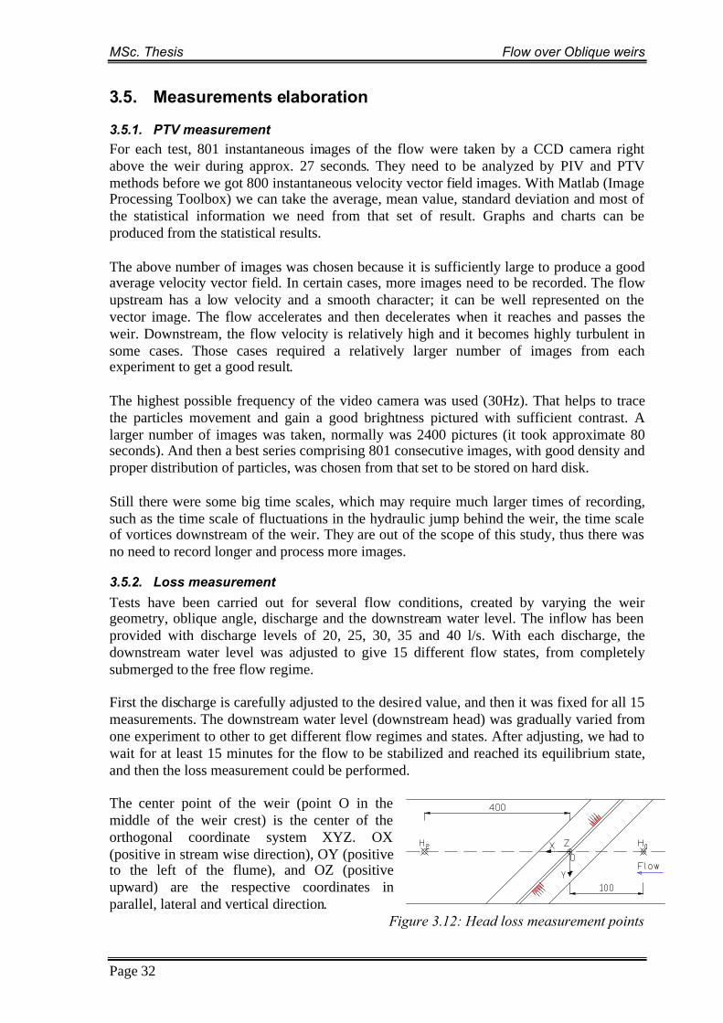
MSc. Thesis Flow over Oblique weirs
Page 32
3.5. Measurements elaboration
3.5.1. PTV measurementFor each test, 801 instantaneous images of the flow were taken by a CCD camera rightabove the weir during approx. 27 seconds. They need to be analyzed by PIV and PTVmethods before we got 800 instantaneous velocity vector field images. With Matlab (ImageProcessing Toolbox) we can take the average, mean value, standard deviation and most ofthe statistical information we need from that set of result. Graphs and charts can beproduced from the statistical results.
The above number of images was chosen because it is sufficiently large to produce a goodaverage velocity vector field. In certain cases, more images need to be recorded. The flowupstream has a low velocity and a smooth character; it can be well represented on thevector image. The flow accelerates and then decelerates when it reaches and passes theweir. Downstream, the flow velocity is relatively high and it becomes highly turbulent insome cases. Those cases required a relatively larger number of images from eachexperiment to get a good result.
The highest possible frequency of the video camera was used (30Hz). That helps to tracethe particles movement and gain a good brightness pictured with sufficient contrast. Alarger number of images was taken, normally was 2400 pictures (it took approximate 80seconds). And then a best series comprising 801 consecutive images, with good density andproper distribution of particles, was chosen from that set to be stored on hard disk.
Still there were some big time scales, which may require much larger times of recording,such as the time scale of fluctuations in the hydraulic jump behind the weir, the time scaleof vortices downstream of the weir. They are out of the scope of this study, thus there wasno need to record longer and process more images.
3.5.2. Loss measurement
Tests have been carried out for several flow conditions, created by varying the weirgeometry, oblique angle, discharge and the downstream water level. The inflow has beenprovided with discharge levels of 20, 25, 30, 35 and 40 l/s. With each discharge, thedownstream water level was adjusted to give 15 different flow states, from completelysubmerged to the free flow regime.
First the discharge is carefully adjusted to the desired value, and then it was fixed for all 15measurements. The downstream water level (downstream head) was gradually varied fromone experiment to other to get different flow regimes and states. After adjusting, we had towait for at least 15 minutes for the flow to be stabilized and reached its equilibrium state,and then the loss measurement could be performed.
The center point of the weir (point O in themiddle of the weir crest) is the center of theorthogonal coordinate system XYZ. OX(positive in stream wise direction), OY (positiveto the left of the flume), and OZ (positiveupward) are the respective coordinates inparallel, lateral and vertical direction.
Figure 3.12: Head loss measurement points
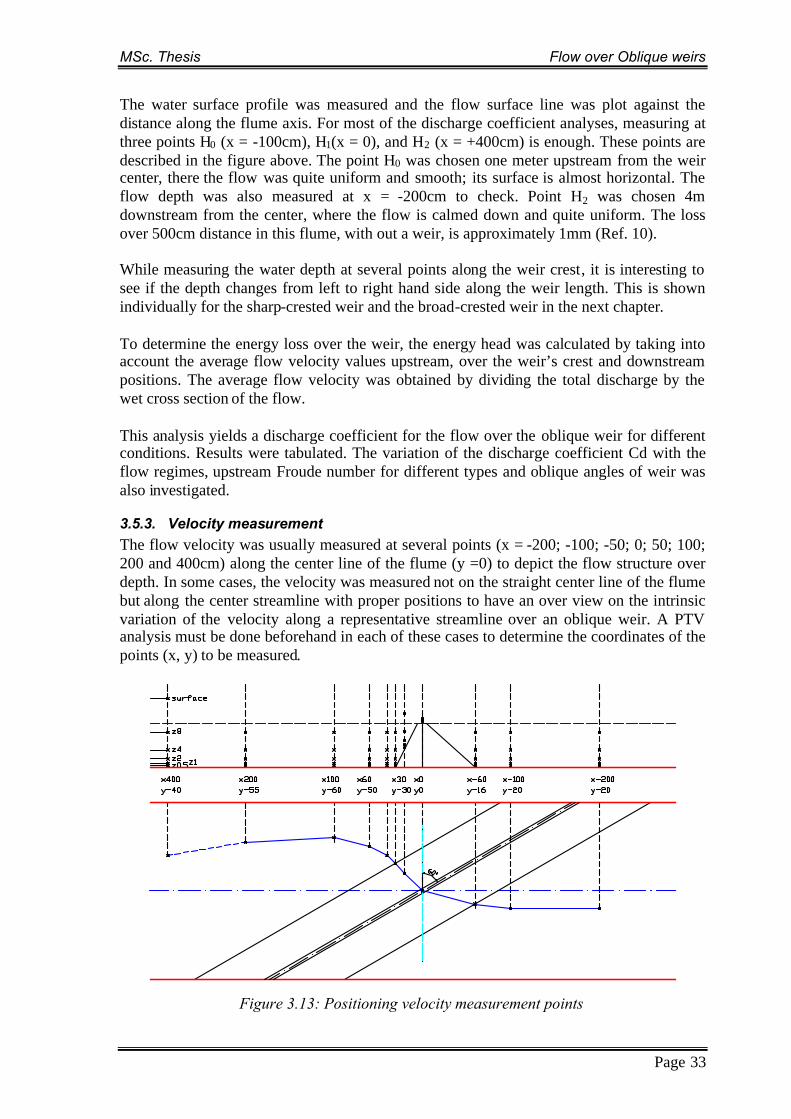
MSc. Thesis Flow over Oblique weirs
Page 33
The water surface profile was measured and the flow surface line was plot against thedistance along the flume axis. For most of the discharge coefficient analyses, measuring atthree points H0 (x = -100cm), H1(x = 0), and H2 (x = +400cm) is enough. These points aredescribed in the figure above. The point H0 was chosen one meter upstream from the weircenter, there the flow was quite uniform and smooth; its surface is almost horizontal. Theflow depth was also measured at x = -200cm to check. Point H2 was chosen 4mdownstream from the center, where the flow is calmed down and quite uniform. The lossover 500cm distance in this flume, with out a weir, is approximately 1mm (Ref. 10).
While measuring the water depth at several points along the weir crest, it is interesting tosee if the depth changes from left to right hand side along the weir length. This is shownindividually for the sharp-crested weir and the broad-crested weir in the next chapter.
To determine the energy loss over the weir, the energy head was calculated by taking intoaccount the average flow velocity values upstream, over the weir’s crest and downstreampositions. The average flow velocity was obtained by dividing the total discharge by thewet cross section of the flow.
This analysis yields a discharge coefficient for the flow over the oblique weir for differentconditions. Results were tabulated. The variation of the discharge coefficient Cd with theflow regimes, upstream Froude number for different types and oblique angles of weir wasalso investigated.
3.5.3. Velocity measurementThe flow velocity was usually measured at several points (x = -200; -100; -50; 0; 50; 100;200 and 400cm) along the center line of the flume (y =0) to depict the flow structure overdepth. In some cases, the velocity was measured not on the straight center line of the flumebut along the center streamline with proper positions to have an over view on the intrinsicvariation of the velocity along a representative streamline over an oblique weir. A PTVanalysis must be done beforehand in each of these cases to determine the coordinates of thepoints (x, y) to be measured.
Figure 3.13: Positioning velocity measurement points
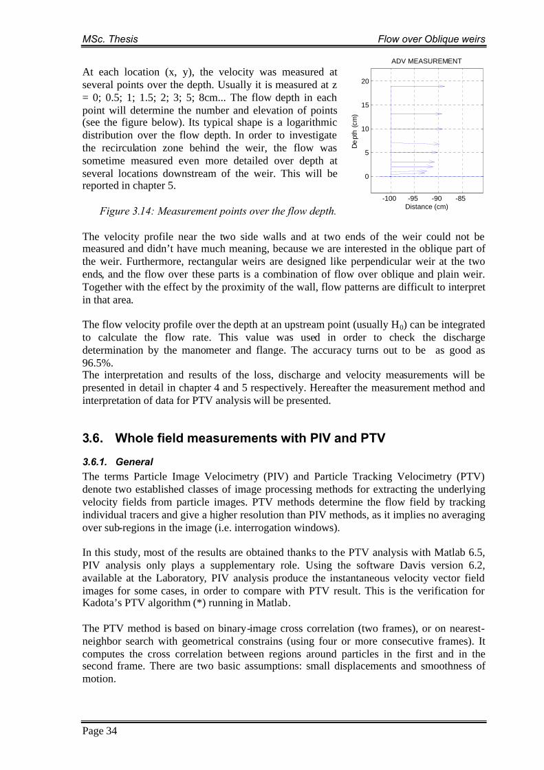
MSc. Thesis Flow over Oblique weirs
Page 34
At each location (x, y), the velocity was measured atseveral points over the depth. Usually it is measured at z= 0; 0.5; 1; 1.5; 2; 3; 5; 8cm... The flow depth in eachpoint will determine the number and elevation of points(see the figure below). Its typical shape is a logarithmicdistribution over the flow depth. In order to investigatethe recirculation zone behind the weir, the flow wassometime measured even more detailed over depth atseveral locations downstream of the weir. This will bereported in chapter 5.
Figure 3.14: Measurement points over the flow depth.
The velocity profile near the two side walls and at two ends of the weir could not bemeasured and didn’t have much meaning, because we are interested in the oblique part ofthe weir. Furthermore, rectangular weirs are designed like perpendicular weir at the twoends, and the flow over these parts is a combination of flow over oblique and plain weir.Together with the effect by the proximity of the wall, flow patterns are difficult to interpretin that area.
The flow velocity profile over the depth at an upstream point (usually H0) can be integratedto calculate the flow rate. This value was used in order to check the dischargedetermination by the manometer and flange. The accuracy turns out to be as good as96.5%.The interpretation and results of the loss, discharge and velocity measurements will bepresented in detail in chapter 4 and 5 respectively. Hereafter the measurement method andinterpretation of data for PTV analysis will be presented.
3.6. Whole field measurements with PIV and PTV
3.6.1. GeneralThe terms Particle Image Velocimetry (PIV) and Particle Tracking Velocimetry (PTV)denote two established classes of image processing methods for extracting the underlyingvelocity fields from particle images. PTV methods determine the flow field by trackingindividual tracers and give a higher resolution than PIV methods, as it implies no averagingover sub-regions in the image (i.e. interrogation windows).
In this study, most of the results are obtained thanks to the PTV analysis with Matlab 6.5,PIV analysis only plays a supplementary role. Using the software Davis version 6.2,available at the Laboratory, PIV analysis produce the instantaneous velocity vector fieldimages for some cases, in order to compare with PTV result. This is the verification forKadota’s PTV algorithm (*) running in Matlab.
The PTV method is based on binary-image cross correlation (two frames), or on nearest-neighbor search with geometrical constrains (using four or more consecutive frames). Itcomputes the cross correlation between regions around particles in the first and in thesecond frame. There are two basic assumptions: small displacements and smoothness ofmotion.
-100 -95 -90 -85
0
5
10
15
20
ADV MEASUREMENT
Distance (cm)
De
pth
(cm
)
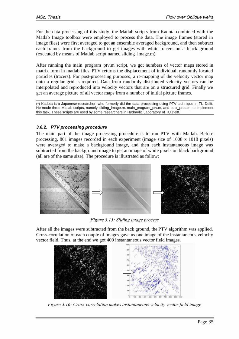
MSc. Thesis Flow over Oblique weirs
Page 35
For the data processing of this study, the Matlab scripts from Kadota combined with theMatlab Image toolbox were employed to process the data. The image frames (stored inimage files) were first averaged to get an ensemble averaged background, and then subtracteach frames from the background to get images with white tracers on a black ground(executed by means of Matlab script named sliding_image.m).
After running the main_program_ptv.m script, we got numbers of vector maps stored inmatrix form in matlab files. PTV returns the displacement of individual, randomly locatedparticles (tracers). For post-processing purposes, a re-mapping of the velocity vector maponto a regular grid is required. Data from randomly distributed velocity vectors can beinterpolated and reproduced into velocity vectors that are on a structured grid. Finally weget an average picture of all vector maps from a number of initial picture frames.
(*) Kadota is a Japanese researcher, who formerly did the data processing using PTV technique in TU Delft.He made three Matlab scripts, namely sliding_image.m, main_program_ptv.m, and post_proc.m, to implementthis task. These scripts are used by some researchers in Hydraulic Laboratory of TU Delft.
3.6.2. PTV processing procedureThe main part of the image processing procedure is to run PTV with Matlab. Beforeprocessing, 801 images recorded in each experiment (image size of 1008 x 1018 pixels)were averaged to make a background image, and then each instantaneous image wassubtracted from the background image to get an image of white pixels on black background(all are of the same size). The procedure is illustrated as follow:
Figure 3.15: Sliding image process
After all the images were subtracted from the back ground, the PTV algorithm was applied.Cross-correlation of each couple of images gave us one image of the instantaneous velocityvector field. Thus, at the end we got 400 instantaneous vector field images.
Figure 3.16: Cross-correlation makes instantaneous velocity vector field image

MSc. Thesis Flow over Oblique weirs
Page 36
Each instantaneous vector image was then recalculated and interpolated to calculate thevectors at fixed grid points. The mesh size was chosen at 20x20 pixels. Then all the fix-grid-points vector-images were averaged to make the final vector field which looks likethis
Figure 3.17: Velocity vector field
The averaged velocity vector field represents the surface velocity field of the flow over theperiod of recording. It gives us an overview of the flow field as well, because the flow inthe experimental flume is a shallow flow with an assumed logarithmic velocity distributionprofile. The image size is 1000x1000 pixels, and the position of the weir can bedetermined. Generally speaking, this image shows clearly the main behavior of the flow:the flow direction, the relative velocity magnitude. Sometimes it even shows someinteresting phenomena observed in the flume, such as the standing surface waves on top ofweir, the vortex and hydraulic jump behind weir, the flow separation and acceleration nearand on top of the weir.
Precise values of the velocity at each grid point can also be known. They were calculatedand stored in several different matrices, upon requirement. Two main matrices are U andV, storing horizontal (perpendicular) and vertical (longitudinal) components of the velocityvectors. Their sizes are 51x51 (in accordance with mesh size of 20 pixels).
3.6.3. CalibrationThe calibration is essential to the result of this PTV analysis. The figures obtained afterrunning PTV with Matlab, like figure 3.17, only presents the vectors with dimension ofpixels per frame (the magnitude of displacement between two consecutive frames inpixels). It is necessary to calibrate this dimension to meter per second (m/s).
Providing two certain points in the flume, the distance in reality (meter), and the distance inimage (pixel) are known. This ratio was then multiply with 30 (the chosen frequency of thecamera). Repeat the above steps every time the weir configuration was changed, we got thecorrection factors for each series of test. Each element of the above matrixes was thenmultiplied with their correlative correction factor. For the sharp-crested weir, the factor K1= 0.046; for the broad-crested weir, K2 = 0.060, for the trapezoidal weir, K3 = 0.0605.
Another artifact derived from the recording procedure is that the picture of the flow isdistorted equally in all four directions, from the center of the image to four corners. Thedeviation of a point on an image increases with its distance to the image center. This

MSc. Thesis Flow over Oblique weirs
artifact can cause a streamline which is straight in fact looks like a curve in the finalvelocity vector field after processing. To deal with that issue, we need a secondarycalibration, which is a whole field calibration.
A squared white panel of the flume size was put into the flume in such a way that the upperface of the panel was horizontal and had the typical elevation of the flow surface duringexperiments. This panel was designed with equally distributed black crosses at grid pointsof a grid size 20 x 20cm. The recorded picture of this panel was distorted in the samemanner as pictures of the flow. After a calibrating procedure done with the software Davis6.2, we got the (correction) calibration matrix to use for other images of vector field duringthe interpretation of PTV data.
3.6.4. Further investigations
The streamlines in the flow can be determined and plot on the vector field image (figure3.18).
Figure 3.18: The streamlinesIt is helpful to take a closer look into what happened along a stream line. Another script canhelp us to draw the streamlines, extract the velocity values along that line, and plot it ongraphs.
It is also helpful to kplain perpendicularcenter line. So it isplot in a graph. Exa
Page 37
now the actual variation of flow velocity along certain lines. As for theweir, ignore the side wall effects, the flow is uniform along the weirinteresting to extract the velocity (components) along that line and to
mples will be presented in the next chapter of the report.
Fig. 3.19: The velocity variation along a streamline

MSc. Thesis Flow over Oblique weirs
Page 38
In order to see the real effect of the obliqueness of the weir, flow velocities weredecomposed into two components parallel and perpendicular to the axis of the weir crest.As we will see later, the perpendicular velocity component contributes a major part to thetotal velocity variation.
3.6.5. LimitsGenerally for each experiment, 801 instantaneous images were taken. They needed to beanalyzed before we got 800 velocity vector field images. Although the computers’ storageand simulation capacity is sufficiently large, it still needs ten to thirty hours to process alldata of one experiment. That restriction in time induces a restriction in the resolution of thefinal vector images. With both PIV and PTV algorithms, we cannot increase the number ofiteration to an infinity large value, and we cannot reduce the grid size of those vectorimages (also the size of interrogation windows) to too small values. That is also notnecessary from the point of view that we only need pictures with certain resolution to viewand interpret the phenomena. The water surface itself also varied considerably, thus a muchfiner resolution of the instantaneous velocity vector field image will be of little use.
3.7. Accuracy and tolerance of measurements
3.7.1. Water depth
Point-gauges were used to measure the height of the free surface and the bed level to±0.1mm. In the case of supercritical flows, the water surface became highly unstablebehind the weir, and sometimes there was air entrainment, these aspects together decreasedthe accuracy to ± 1mm. Far downstream (i.e. 4 meters from the weir center), the flowsurface calmed down and the accuracy of the depth measurement can be ensured as normal(±0.1mm).
3.7.2. VelocityThe velocity was measured by an ADV and an EMF, both were carefully calibrated. Theonly uncertainty for the velocity measurement is the quality of the signal for the ADV; andthe curvature of the flow underneath the probe of the EMF.
The shape and size of the EMF probe caused the flow streamlines to be curved from itsoriginal shape. Although the EMF was designed with rather small dimension and mountedin a best manner, this still affected the flow to some extends. The strongest effect occurredwhen the flow depth was small, especially on top of the weir.
The size of the ADV probe is smaller than the above and the probe was usually mounted5cm downstream of the measuring volume, so this hardly affected the flow. The maindisturbance to the flow is the hydrogen bubble generator located some 40cm upstream ofthe measuring volume. This effect was also minimized by the design of the bubblegenerator.
Another source of errors for measurements by the ADV is the signal strength. Disturbanceto the flow like a small bubble or a small change in density of the tiny hydrogen bubblecloud could cause the signal strength to vary. A bigger accumulated bubble can produce apeak or drop in the recorded signal. These errors can be avoided by introducing a filterfunction into the processing procedure in Matlab. Usually the data with quality lower than70 counts are ignored during this process.
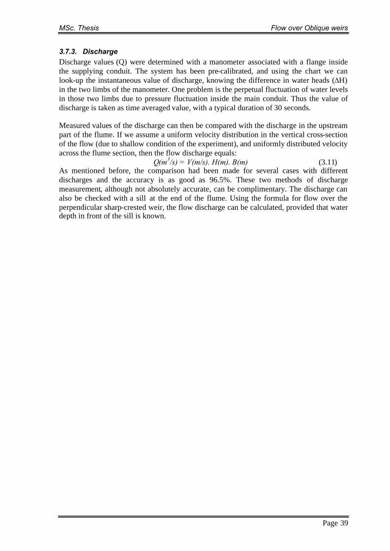
MSc. Thesis Flow over Oblique weirs
Page 39
3.7.3. DischargeDischarge values (Q) were determined with a manometer associated with a flange insidethe supplying conduit. The system has been pre-calibrated, and using the chart we canlook-up the instantaneous value of discharge, knowing the difference in water heads (H)in the two limbs of the manometer. One problem is the perpetual fluctuation of water levelsin those two limbs due to pressure fluctuation inside the main conduit. Thus the value ofdischarge is taken as time averaged value, with a typical duration of 30 seconds.
Measured values of the discharge can then be compared with the discharge in the upstreampart of the flume. If we assume a uniform velocity distribution in the vertical cross-sectionof the flow (due to shallow condition of the experiment), and uniformly distributed velocityacross the flume section, then the flow discharge equals:
Q(m3/s) = V(m/s). H(m). B(m) (3.11)As mentioned before, the comparison had been made for several cases with differentdischarges and the accuracy is as good as 96.5%. These two methods of dischargemeasurement, although not absolutely accurate, can be complimentary. The discharge canalso be checked with a sill at the end of the flume. Using the formula for flow over theperpendicular sharp-crested weir, the flow discharge can be calculated, provided that waterdepth in front of the sill is known.
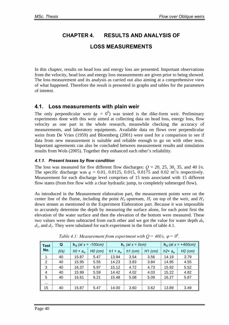
MSc. Thesis Flow over Oblique weirs
Page 40
CHAPTER 4. RESULTS AND ANALYSIS OF
LOSS MEASUREMENTS
In this chapter, results on head loss and energy loss are presented. Important observationsfrom the velocity, head loss and energy loss measurements are given prior to being showed.The loss measurement and its analysis as carried out also aiming at a comprehensive viewof what happened. Therefore the result is presented in graphs and tables for the parametersof interest.
4.1. Loss measurements with plain weirThe only perpendicular weir (= 00) was tested is the dike-form weir. Preliminaryexperiments done with this weir aimed at collecting data on head loss, energy loss, flowvelocity as one part in the whole research, meanwhile checking the accuracy ofmeasurements, and laboratory equipments. Available data on flows over perpendicularweirs from De Vries (1959) and Bloemberg (2001) were used for a comparison to see ifdata from new measurement is suitable and reliable enough to go on with other tests.Important agreements can also be concluded between measurement results and simulationresults from Wols (2005). Together they enhanced each other’s reliability.
4.1.1. Present losses by flow condition
The loss was measured for five different flow discharges: Q = 20, 25, 30, 35, and 40 l/s.The specific discharge was q = 0.01, 0.0125, 0.015, 0.0175 and 0.02 m2/s respectively.Measurement for each discharge level comprises of 15 tests associated with 15 differentflow states (from free flow with a clear hydraulic jump, to completely submerged flow).
As introduced in the Measurement elaboration part, the measurement points were on thecenter line of the flume, including the point H0 upstream, H1 on top of the weir, and H2down stream as mentioned in the Experiment Elaboration part. Because it was impossibleto accurately determine the depth by measuring the surface alone, for each point first theelevation of the water surface and then the elevation of the bottom were measured. Thesetwo values were then subtracted from each other and we got the value for water depth d0,d1, and d2. They were tabulated for each experiment in the form of table 4.1.
Table 4.1: Measurement from experiment with Q = 40l/s, = 00.
Q h0 (at x = -100cm) h1 (at x = 0cm) h2 (at x = +400cm)TestNo. (l/s) h0 + aw H0 (cm) h1 + aw h1 (cm) H1 (cm) h2+ aw H2 (cm)1 40 15.87 5.47 13.94 3.54 3.56 14.19 3.792 40 15.95 5.55 14.23 3.83 3.84 14.95 4.553 40 16.37 5.97 15.12 4.72 4.73 15.92 5.524 40 15.99 5.59 14.42 4.02 4.03 15.22 4.825 40 16.61 6.21 15.48 5.08 5.09 16.27 5.87...15 40 15.87 5.47 14.00 3.60 3.62 13.89 3.49

MSc. Thesis Flow over Oblique weirs
Page 41
The energy loss was coupled with the head loss by taking into account the velocity heads(v2/2g) at measured points, where v is the cross-section averaged flow velocity (v=q/d).Because the velocity head is proportional to the square of the velocity, it thus attains itsmaximum value at the weir crest, where the depth d is smallest. The typical value of thevelocity head at this position was 0.015cm. At other measured points it was much smallerand only accounted for approximately 0.50/00 of the energy head. Usually the velocity headis negligible small and the energy loss can be interpreted as head loss.
Following, the head loss will be present with flow conditions in figure 4.1
0
1
2
3
4
5
6
7
0.0 0.2 0.4 0.6 0.8 1.0 1.2
Fr1
Hea
dlo
ss(c
m)
Q = 40 l/sQ = 35 l/sQ = 30 l/sQ = 25 l/sQ = 20 l/s
Figure 4.1: Relation between head loss and Froude number above the weir, = 00
As can be seen from the measurement data, the influences of some main hydraulicparameters to the head loss can be summarized as follow:
- With the same discharge, the head loss decreases with the increase of thedownstream water head (increase the submergence). The decreasing rate isinsignificant when the downstream water head is bigger than half the weir height.
- With the same flow state (same Froude number on top of the weir), the loss seemsto be independent from the changes in discharge.
- With the same downstream water head, the higher the discharge the bigger the loss.The same conclusion can be made for two flows with the same submergence.
- At the free flow state, the head loss increases as much as the downstream headdecreases; the relation between them is linear.

MSc. Thesis Flow over Oblique weirs
Page 42
0
1
2
3
4
5
6
7
0.8 1.0 1.2 1.4 1.6 1.8 2.0d2 /aw
Hea
dlo
ss(c
m) Q = 40 l/s
Q = 35 l/sQ = 30 l/sQ = 25 l/sQ = 20 l/s
Figure 4.2: Relation between head loss and the relative downstream water depth, = 00
When the downstream water head was high, the flow was usually submerged and the lossin water head from upstream to downstream section was only in order of 1mm. Taken intoaccount the loss in free flume (without any weirs) over five meter distance is about 1mm(see chapter 2), we can hardly see any effect of the present of the dike-form weir.
By decreasing the downstream water level, gradually the flow turned to undulated and thenemerged, the losses increased as well. In these cases, the flow is much more turbulent, thevelocity fluctuated stronger and causes the energy to be dissipated more significantly. Theloss can be as high as 50% of the upstream water head.
4.1.2. Analysis of losses
Discharge coefficients from measurementsThe measurement data can be used to calculate some dependent flow parameters. The mostimportant one is the discharge coefficient. It represents the flow rate over the weir andreflects the losses over the weir. Following the discharge coefficient (Cd) and the dischargereduction coefficient (C*) will be present together with the flow conditions.It is shown that Cd is a function of different parameters such as H0, S. However there is noclear and simple relation between them. The empirical of Villemonte (1947) fits in instead.
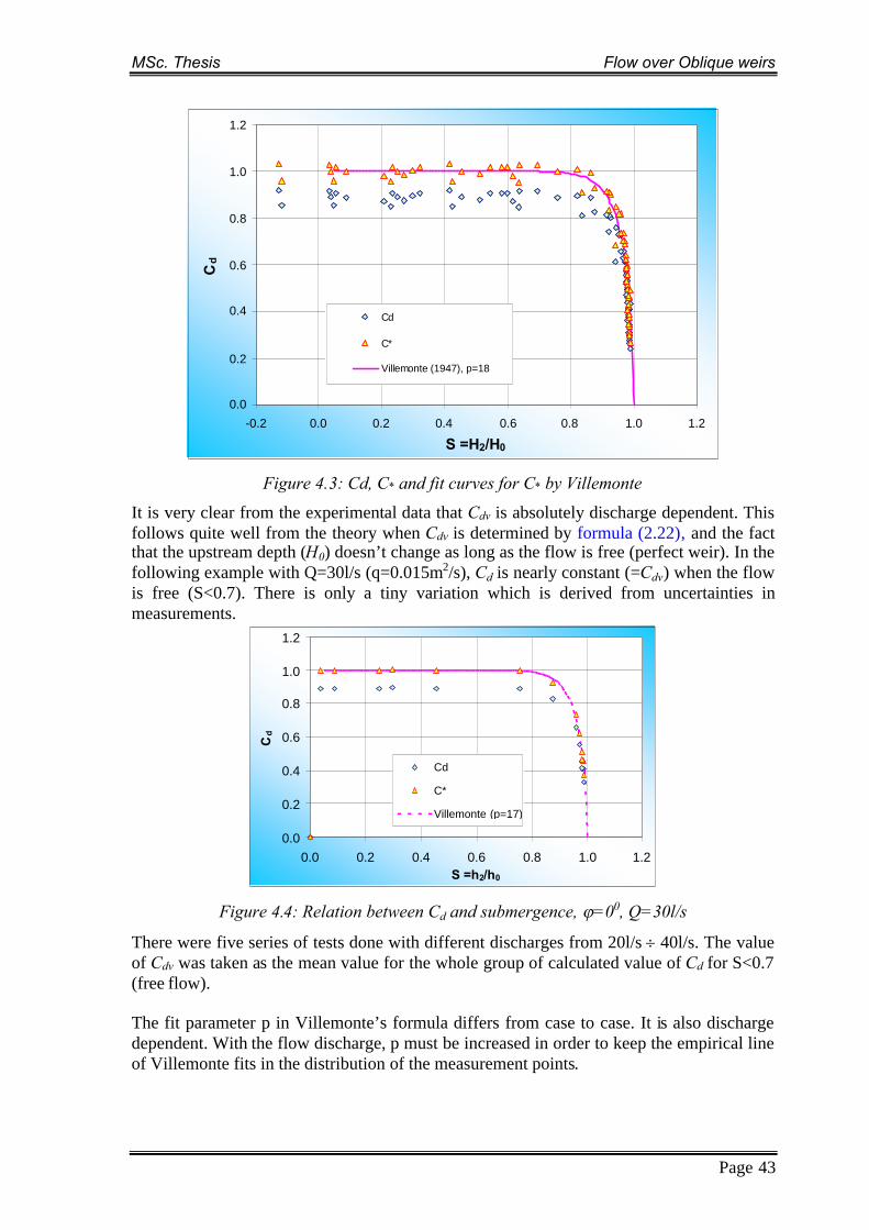
MSc. Thesis Flow over Oblique weirs
Page 43
0.0
0.2
0.4
0.6
0.8
1.0
1.2
-0.2 0.0 0.2 0.4 0.6 0.8 1.0 1.2
S =H2/H0
Cd
Cd
C*
Villemonte (1947), p=18
Figure 4.3: Cd, C* and fit curves for C* by Villemonte
It is very clear from the experimental data that Cdv is absolutely discharge dependent. Thisfollows quite well from the theory when Cdv is determined by formula (2.22), and the factthat the upstream depth (H0) doesn’t change as long as the flow is free (perfect weir). In thefollowing example with Q=30l/s (q=0.015m2/s), Cd is nearly constant (=Cdv) when the flowis free (S<0.7). There is only a tiny variation which is derived from uncertainties inmeasurements.
0.0
0.2
0.4
0.6
0.8
1.0
1.2
0.0 0.2 0.4 0.6 0.8 1.0 1.2S =h2/h0
Cd
Cd
C*
Villemonte (p=17)
Figure 4.4: Relation between Cd and submergence, =00, Q=30l/s
There were five series of tests done with different discharges from 20l/s 40l/s. The valueof Cdv was taken as the mean value for the whole group of calculated value of Cd for S<0.7(free flow).
The fit parameter p in Villemonte’s formula differs from case to case. It is also dischargedependent. With the flow discharge, p must be increased in order to keep the empirical lineof Villemonte fits in the distribution of the measurement points.

MSc. Thesis Flow over Oblique weirs
Page 44
0
5
10
15
20
25
10 20 30 40 50Q (l/s)
Fit
pa
ram
ete
rp
p ~ Q
Figure 4.5: Relation between fit parameter and discharge
The relation between discharge coefficient and the Froude number above the weir has beenestablished in chapter 2. The Froude number is a dimensionless parameter that is unique foreach flow state. From the experimental data, the discharge coefficient can be plot againstthe Froude number above the weir for each test. Final result for the perpendicular weir isgiven below together with the relation in equation (2.38): energy conservation.
0.0
0.2
0.4
0.6
0.8
1.0
1.2
0.0 0.2 0.4 0.6 0.8 1.0 1.2Fr1
Cd Cd
C*
Energy balance
Fig 4.6: Relation between discharge coefficient and Froude number above the weir, = 0
The result appears very sensitive to the weir height, thus the realistic value of weir heightwas checked and obtained by several different methods. The precise value of weir height inthe flume is aw = 10.4cm.
From the momentum balance, the relation between the submergence and the Froudenumber above the weir has been established for different discharges. The measurementdata from all tests are plotted on the same graph. They show a good agreement with thetheoretical prediction (equation 2.41), except the deviation at high Froude number (freeflow, perfect weir). The following figure illustrates their relation.
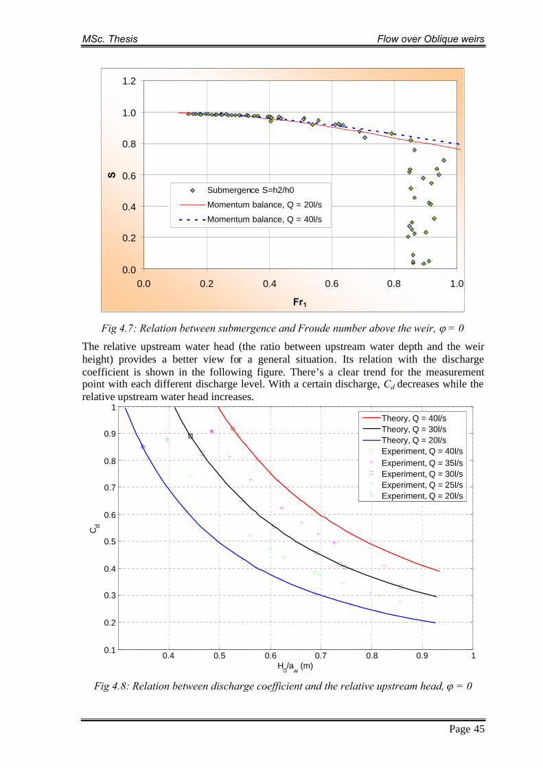
MSc. Thesis Flow over Oblique weirs
Page 45
0.0
0.2
0.4
0.6
0.8
1.0
1.2
0.0 0.2 0.4 0.6 0.8 1.0
Fr1
S
Submergence S=h2/h0
Momentum balance, Q = 20l/s
Momentum balance, Q = 40l/s
Fig 4.7: Relation between submergence and Froude number above the weir, = 0
The relative upstream water head (the ratio between upstream water depth and the weirheight) provides a better view for a general situation. Its relation with the dischargecoefficient is shown in the following figure. There’s a clear trend for the measurementpoint with each different discharge level. With a certain discharge, Cd decreases while therelative upstream water head increases.
0.4 0.5 0.6 0.7 0.8 0.9 10.1
0.2
0.3
0.4
0.5
0.6
0.7
0.8
0.9
1
H0/a
w(m)
Cd
Theory, Q = 40l/sTheory, Q = 30l/sTheory, Q = 20l/sExperiment, Q = 40l/sExperiment, Q = 35l/sExperiment, Q = 30l/sExperiment, Q = 25l/sExperiment, Q = 20l/s
Fig 4.8: Relation between discharge coefficient and the relative upstream head,= 0
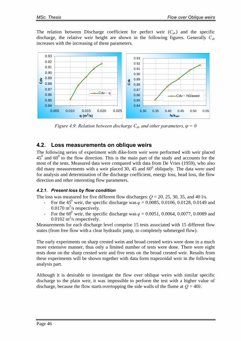
MSc. Thesis Flow over Oblique weirs
Page 46
The relation between Discharge coefficient for perfect weir (Cdv) and the specificdischarge, the relative weir height are shown in the following figures. Generally Cdvincreases with the increasing of these parameters.
0.840.85
0.860.87
0.88
0.890.90
0.910.92
0.93
0.005 0.010 0.015 0.020 0.025q (m2/s)
Cdv
Cdv ~ q
0.84
0.85
0.86
0.87
0.88
0.89
0.90
0.91
0.92
0.93
0.30 0.35 0.40 0.45 0.50 0.55h0/aweir
Cdv
Cdv ~ h0/aweir
Figure 4.9: Relation between discharge Cdv and other parameters,= 0
4.2. Loss measurements on oblique weirsThe following series of experiment with dike-form weir were performed with weir placed450 and 600 to the flow direction. This is the main part of the study and accounts for themost of the tests. Measured data were compared with data from De Vries (1959), who alsodid many measurements with a weir placed 30, 45 and 600 obliquely. The data were usedfor analysis and determination of the discharge coefficient, energy loss, head loss, the flowdirection and other interesting flow parameters.
4.2.1. Present loss by flow conditionThe loss was measured for five different flow discharges: Q = 20, 25, 30, 35, and 40 l/s.
- For the 450 weir, the specific discharge was q = 0.0085, 0.0106, 0.0128, 0.0149 and0.0170 m2/s respectively.
- For the 600 weir, the specific discharge was q = 0.0051, 0.0064, 0.0077, 0.0089 and0.0102 m2/s respectively.
Measurements for each discharge level comprise 15 tests associated with 15 different flowstates (from free flow with a clear hydraulic jump, to completely submerged flow).
The early experiments on sharp crested weirs and broad crested weirs were done in a muchmore extensive manner, thus only a limited number of tests were done. There were eighttests done on the sharp crested weir and five tests on the broad crested weir. Results fromthese experiments will be shown together with data form trapezoidal weir in the followinganalysis part.
Although it is desirable to investigate the flow over oblique weirs with similar specificdischarge to the plain weir, it was impossible to perform the test with a higher value ofdischarge, because the flow starts overtopping the side walls of the flume at Q = 40l/.
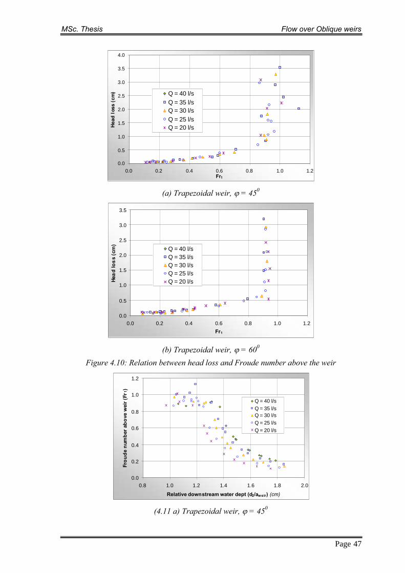
MSc. Thesis Flow over Oblique weirs
Page 47
0.0
0.5
1.0
1.5
2.0
2.5
3.0
3.5
4.0
0.0 0.2 0.4 0.6 0.8 1.0 1.2Fr1
Hea
dlo
ss(c
m) Q = 40 l/s
Q = 35 l/sQ = 30 l/sQ = 25 l/sQ = 20 l/s
(a) Trapezoidal weir, = 450
0.0
0.5
1.0
1.5
2.0
2.5
3.0
3.5
0.0 0.2 0.4 0.6 0.8 1.0 1.2
Fr1
Hea
dlo
ss
(cm
)
Q = 40 l/sQ = 35 l/sQ = 30 l/sQ = 25 l/sQ = 20 l/s
(b) Trapezoidal weir, = 600
Figure 4.10: Relation between head loss and Froude number above the weir
0.0
0.2
0.4
0.6
0.8
1.0
1.2
0.8 1.0 1.2 1.4 1.6 1.8 2.0
Relative downstream water dept (d2/aweir) (cm)
Fro
ud
en
umb
erab
ove
wei
r(F
r1)
Q = 40 l/sQ = 35 l/sQ = 30 l/sQ = 25 l/sQ = 20 l/s
(4.11 a) Trapezoidal weir, = 450

MSc. Thesis Flow over Oblique weirs
Page 48
0.0
0.1
0.2
0.3
0.4
0.5
0.6
0.7
0.8
0.9
1.0
0.8 1.0 1.2 1.4 1.6 1.8 2.0
Relative downstream water depth (h2/aweir) (cm)
Fro
ud
en
um
be
rab
ov
ew
eir
(Fr1
)
Q = 40 l/sQ = 35 l/sQ = 30 l/sQ = 25 l/sQ = 20 l/s
(4.11 b) Trapezoidal weir, = 600
Figure 4.11: Relation between Fr1 and the relative downstream water depth
- The overall qualitative conclusions about head loss, energy loss and their relation toother hydraulic parameters appear to be as the same with the case of a perpendiculartrapezoidal weir (=00). The trend of changing losses associates with the flowregime), the loss seems to be independent from the changes in discharge.
- With the same downstream water head, the higher the discharge the bigger the loss.The same conclusion can be drawn for two flows with the same submergence.
- At the free flow state, the head loss increases as much as the downstream headdecreases; the relation between them is linear.
The only difference is that the magnitude of loss changes when the oblique angle changes.Some brief remarks are:
- With the same submergence, the loss is smallest when =600 and is biggest when=00 .
- At a low value of the Froude number, there is no significant difference betweenlosses for different oblique angle. Although the loss is slightly higher when theoblique angle is bigger.
When the Froude number is low (high submergence or submerged flow), the loss in waterhead from upstream to downstream section was also small, in the order of 1mm. Taken intoaccount the loss in free flume (without any weirs) over five meter distance is about 1mm(see chapter 2), the effect of the present of the oblique trapezoidal weir can hardly be seen.
Similar to the perpendicular weir, by decreasing the downstream water level gradually theflow turned to undulating and then emerged, the losses increased as well. The loss in thecase of an undulating flow is usually in the order of 0.5cm. The loss in a free flow can bemuch higher.

MSc. Thesis Flow over Oblique weirs
Page 49
4.2.2. Analysis of loss measurement
4.2.2.1. Discharge coefficients from measurementsThe measurement data from oblique weirs were use to calculate the discharge coefficientbased on the formulas from chapter 2 and plot in three figures below. Both the dischargecoefficient (Cd) and the discharge reduction coefficient (C*) are of interest.
The discharge coefficient was calculated from a modification of the basic equation forweirs, in which the length of the weir (L) was used instead of the channel width (B):
2/30.
32
.32
HgL
QCd (4.1)
We consider the specific discharge of the flow over the whole length of the weir, not thewhole width of the flume (as we usually do for a perpendicular weir). This is a differenceof a factor 1/cos(). Physically it means that the flow component perpendicular to the weircrest is of interest. Later on we will only consider the velocity component that isperpendicular to the weir crest.The distribution of C* points from measurement for trapezoidal weirs is best fitted by theempirical formula of Villemonte (1947) with different value of p. Other empirical relationsintroduced in chapter 2 don’t fit anymore (see figure 4.12 a, b). The value of p decreaseswhen the oblique angle increases (p=18 for =00, p=16 for =450, and p=15 for =600).
At low submergence (S 0.7), Cd is constant for each discharge level. The mean value ofthe whole set of measurement points with S 0.7 was chosen as Cdv.
The value of Cdv is not only discharge dependent (as discussed earlier), but also depends onthe angle (the configuration of the weir in general). As can be interpreted from the results,Cd slightly decreases when increasing the oblique from 00 to 600. This fact and itsinfluence on the discharge capacity will be further discussed at the end of this chapter.
0.0
0.2
0.4
0.6
0.8
1.0
1.2
0.0 0.2 0.4 0.6 0.8 1.0 1.2S =H2/H0
Cd
Cd
C*
Villemonte (1947), p=16
Seida & Quarashi
Villemonte (Kolkman 1989)
Varshney & Mohanty
(4.12 a) Trapezoidal weir, = 450
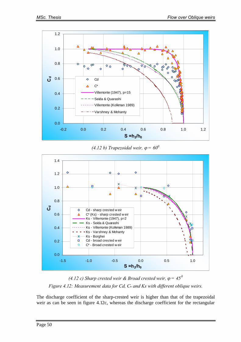
MSc. Thesis Flow over Oblique weirs
Page 50
0.0
0.2
0.4
0.6
0.8
1.0
1.2
-0.2 0.0 0.2 0.4 0.6 0.8 1.0 1.2
S =h2/h0
Cd
Cd
C*
Villemonte (1947), p=15
Seida & Quarashi
Villemonte (Kolkman 1989)
Varshney & Mohanty
(4.12 b) Trapezoidal weir, = 600
0.0
0.2
0.4
0.6
0.8
1.0
1.2
1.4
-1.5 -1.0 -0.5 0.0 0.5 1.0
S =h2/h0
Cd
Cd - sharp crested w eirC* (Ks) - sharp crested w eirKs - Villemonte (1947), p=2Ks - Seida & QuarashiKs - Villemonte (Kolkman 1989)Ks - Varshney & MohantyKs - BorgheiCd - broad crested w eirC* - Broad crested w eir
(4.12 c) Sharp crested weir & Broad crested weir, = 450
Figure 4.12: Measurement data for Cd, C* and Ks with different oblique weirs.
The discharge coefficient of the sharp-crested weir is higher than that of the trapezoidalweir as can be seen in figure 4.12c, whereas the discharge coefficient for the rectangular

MSc. Thesis Flow over Oblique weirs
Page 51
broad-crested weir is always 1. This is explainable because the broad-crested weir is a longweir, and the Froude number on the crest in the case of a critical flow is exactly 1.
It is shown in figure 4.12c that the empirical relations used to determine the dischargereduction coefficient (C*) or the submergence coefficient (KS), which were constructed fora perpendicular sharp crested, mostly fit in the case of a oblique sharp crested weir(=450). Good agreement between empirical lines and measurement points was found withlow Froude number.
For the oblique rectangular broad crested weir, the best fit distribution for the measurementpoints is the empirical formula from Villemonte (1947) with the fit parameter p=4.
When the fit parameter p = 2, the empirical line from the formula of Villemonte (1947)coincide with the empirical line from his formula in 1989. These two lines fit thedistribution of the measurement points of KS, and so do other lines from Borghei, Seida &Quarashi. For the sharp-crested weir which was tested, the only line which fits least is theline from Varshney & Mohanty.
0.0
0.2
0.4
0.6
0.8
1.0
1.2
0.0 0.2 0.4 0.6 0.8 1.0 1.2 1.4Fr1
Cd Cd
C*
Energy balance
(4.13 a) Trapezoidal weir, = 450
0.0
0.2
0.4
0.6
0.8
1.0
1.2
0.0 0.2 0.4 0.6 0.8 1.0 1.2
Fr1
Cd
Cd
C*
Energy balance
(4.13 b) Trapezoidal weir, = 600
Fig 4.13: Relation between discharge coefficient and Froude number above the weir

MSc. Thesis Flow over Oblique weirs
Page 52
Figure 4.13a and b show the relations between Cd and Fr1, together with the theoretical linefor this relation. This line was constructed based on the assumption of energy conservationbetween one upstream section and one section above the weir crest.
The submergence was plotted against the Froude number above the weir in figure 4.14.Measurement data from all tests with different discharge levels (20, 25, 30, 35 and 40l/s)were plotted together. The distribution of the measurement points has a relatively goodagreement with the two theoretical lines constructed on the basis of momentumconservation downstream of the weir. However there is a relatively large scatter ofmeasurement data at high Froude number (free flow) as expected.
0.0
0.2
0.4
0.6
0.8
1.0
1.2
0.0 0.2 0.4 0.6 0.8 1.0
Fr1
S
A measurement data
Momentum Balance (Q=20l/s)
Momentum Balance (Q=40l/s)
(4.14 a) Trapezoidal weir, = 450
0.0
0.2
0.4
0.6
0.8
1.0
1.2
0.0 0.2 0.4 0.6 0.8 1.0
Fr1
S
A measurement data
Momentum balance, Q=20l/s
Momentum balance, Q=40l/s
(4.14 b) Trapezoidal weir, = 600
Figure 4.14: Relation between submergence and Froude number above the weir
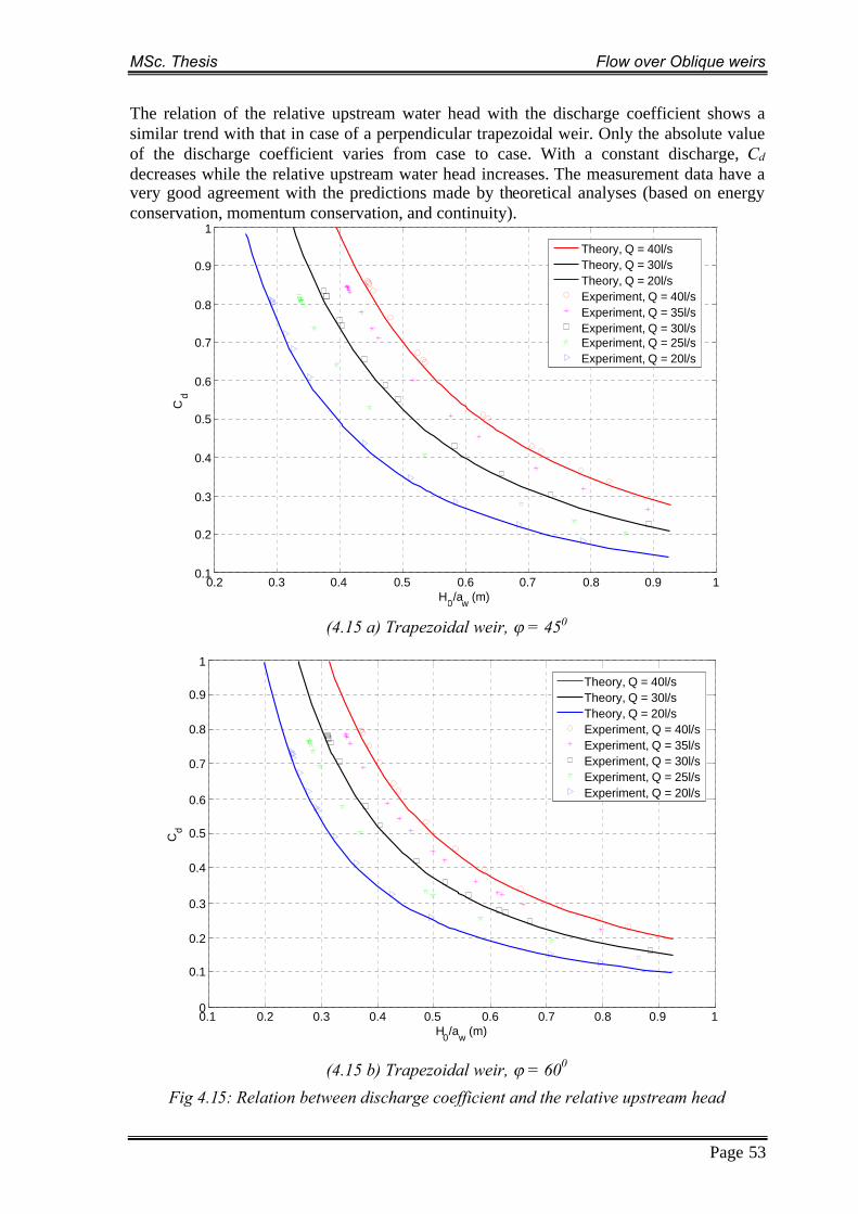
MSc. Thesis Flow over Oblique weirs
Page 53
The relation of the relative upstream water head with the discharge coefficient shows asimilar trend with that in case of a perpendicular trapezoidal weir. Only the absolute valueof the discharge coefficient varies from case to case. With a constant discharge, Cd
decreases while the relative upstream water head increases. The measurement data have avery good agreement with the predictions made by theoretical analyses (based on energyconservation, momentum conservation, and continuity).
0.2 0.3 0.4 0.5 0.6 0.7 0.8 0.9 10.1
0.2
0.3
0.4
0.5
0.6
0.7
0.8
0.9
1
H0/a
w(m)
Cd
Theory, Q = 40l/sTheory, Q = 30l/sTheory, Q = 20l/sExperiment, Q = 40l/sExperiment, Q = 35l/sExperiment, Q = 30l/sExperiment, Q = 25l/sExperiment, Q = 20l/s
(4.15 a) Trapezoidal weir, = 450
0.1 0.2 0.3 0.4 0.5 0.6 0.7 0.8 0.9 10
0.1
0.2
0.3
0.4
0.5
0.6
0.7
0.8
0.9
1
H0/aw (m)
Cd
Theory, Q = 40l/sTheory, Q = 30l/sTheory, Q = 20l/sExperiment, Q = 40l/sExperiment, Q = 35l/sExperiment, Q = 30l/sExperiment, Q = 25l/sExperiment, Q = 20l/s
(4.15 b) Trapezoidal weir, = 600
Fig 4.15: Relation between discharge coefficient and the relative upstream head

MSc. Thesis Flow over Oblique weirs
Page 54
The relations between Discharge coefficient for perfect weir (Cdv) and the specificdischarge (q), the relative weir height (H0/aw) are shown in the following table.
Table 4.2: Cdv with different discharges and different oblique angle
Q B L q Cd p h0 H0 aw H0/aw
l/s degr. m m m2/s - - cm cm cm -20 0 2 2 0.010 0.852 14 14.02 3.62 10.4 0.34825 0 2 2 0.013 0.877 16 14.52 4.12 10.4 0.39630 0 2 2 0.015 0.892 17 15.00 4.60 10.4 0.44235 0 2 2 0.018 0.910 19 15.43 5.03 10.4 0.48440 0 2 2 0.020 0.917 20 15.87 5.47 10.4 0.52620 45 2 2.83 0.007 0.806 12 13.18 2.98 10.2 0.29225 45 2 2.83 0.009 0.820 14 13.62 3.42 10.2 0.33530 45 2 2.83 0.011 0.833 16 14.02 3.82 10.2 0.37535 45 2 2.83 0.012 0.843 19 14.40 4.20 10.2 0.41240 45 2 2.83 0.014 0.855 20 14.75 4.55 10.2 0.44620 60 2 3.94 0.005 0.731 11 12.85 2.55 10.3 0.24825 60 2 3.94 0.006 0.765 13 13.17 2.87 10.3 0.27930 60 2 3.94 0.008 0.777 15 13.51 3.21 10.3 0.31235 60 2 3.94 0.009 0.786 16 13.83 3.53 10.3 0.34340 60 2 3.94 0.010 0.798 18 14.12 3.82 10.3 0.371
It can be seen that Cdv slightly decreases with the increasing of the specific discharge andthe relative weir height. This can be qualitatively explained by the fact that the bigger theobliqueness of the weir is, the more unfavorable the flow condition is. Figure 4.16aillustrate the relation between Cd and the relative upstream energy head, and figure 4.16billustrates the dependency of Cd on the specific discharge.
0.4
0.5
0.6
0.7
0.8
0.9
1.0
0.000 0.005 0.010 0.015 0.020 0.025
q (m2/s)
Cd
Phi0phi45
phi60
(a) (b)
Figure 4.16: Discharge coefficient with different oblique angles
Although the discharge coefficient for the perfect weir (Cdv) slightly decreases, theeffective length of the weir increases significantly (by 1/cos()) with increasing the angleof obliqueness.
)cos(BL (4.2)
0.4
0.5
0.6
0.7
0.8
0.9
1.0
0.2 0.3 0.4 0.5 0.6
H0/aw
Cd
Phi0phi45
phi60

MSc. Thesis Flow over Oblique weirs
Page 55
where B is the channel width (B=2m), is the oblique angle of the weir.
Together, the flow rate over the weir increases significantly (a factor of L*Cdv) when theoblique angle increases (in the case of free flows). For submerged flow, this trend stays thesame, keeping in mind the discharge reduction factor C* determined by Villemonteformula.
The data and analysis from this chapter asserts the increase of weir discharge capacitywhen the oblique angle is increased.
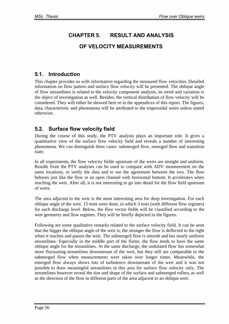
MSc. Thesis Flow over Oblique weirs
Page 56
CHAPTER 5. RESULT AND ANALYSIS
OF VELOCITY MEASUREMENTS
5.1. IntroductionThis chapter provides us with information regarding the measured flow velocities. Detailedinformation on flow pattern and surface flow velocity will be presented. The oblique angleof flow streamlines is related to the velocity component analysis, its trend and variation isthe object of investigation as well. Besides, the vertical distribution of flow velocity will beconsidered. They will either be showed here or in the appendices of this report. The figures,data, characteristic and phenomena will be attributed to the trapezoidal weirs unless statedotherwise.
5.2. Surface flow velocity fieldDuring the course of this study, the PTV analysis plays an important role. It gives aquantitative view of the surface flow velocity field and reveals a number of interestingphenomena. We can distinguish three cases: submerged flow, emerged flow and transitionstate.
In all experiments, the flow velocity fields upstream of the weirs are straight and uniform.Results from the PTV analyses can be used to compare with ADV measurement on thesame locations, to verify the data and to see the agreement between the two. The flowbehaves just like the flow in an open channel with horizontal bottom. It accelerates whenreaching the weir. After all, it is not interesting to go into detail for the flow field upstreamof weirs.
The area adjacent to the weir is the most interesting area for deep investigation. For eachoblique angle of the weir, 15 tests were done, in which 3 tests (with different flow regimes)for each discharge level. Below, the flow vector fields will be classified according to theweir geometry and flow regimes. They will be briefly depicted in the figures.
Following are some qualitative remarks related to the surface velocity field. It can be seenthat the bigger the oblique angle of the weir is, the stronger the flow is deflected to the rightwhen it reaches and passes the weir. The submerged flow is smooth and has nearly uniformstreamlines. Especially in the middle part of the flume, the flow tends to have the sameoblique angle for the streamlines. At the same discharge, the undulated flow has somewhatmore fluctuating streamlines downstream of the weir, but they still are comparable to thesubmerged flow when measurements were taken over longer times. Meanwhile, theemerged flow always shows lots of turbulence downstream of the weir and it was notpossible to draw meaningful streamlines in this area for surface flow velocity only. Thestreamlines however reveal the size and shape of the surface and submerged rollers, as wellas the direction of the flow in different parts of the area adjacent to an oblique weir.

MSc. Thesis Flow over Oblique weirs
Page 57
5.2.1. Perpendicular weir (= 00)Following the three distinction flow regimes (as have been classified in chapter 2) will bepresented. The figures below depict the free surface flow velocity field, thus providing anoverview of the flow in the flume as well as the flow over a prototype with the sameconditions. However the figures also reveal some interesting phenomena, for example thehydraulic jump (in the case of an emerged flow), the development of undulations on theflow surface and its variation over the flume width (in the case of a undulated flow)...
0 0.5 1 1.5 2
0.2
0.4
0.6
0.8
1
1.2
1.4
1.6
1.8
2
Figure 5.1: Flow velocity vector field,=00, Q=30l/s, Emerged flow
0 0.5 1 1.5 2 2.5
0.2
0.4
0.6
0.8
1
1.2
1.4
1.6
1.8
2
Figure 5.2: Flow velocity vector field, =00, Q=30l/s, Undulated flow
Hydraulic jump
weir crest
Flow direction

MSc. Thesis Flow over Oblique weirs
Page 58
0 0.5 1 1.5 2 2.5
0.2
0.4
0.6
0.8
1
1.2
1.4
1.6
1.8
2
Figure 5.3: Flow velocity vector field, =00 , Q=25l/s, Submerged flow
The distances in figures are in meter, the flow direction is from the top to the bottom. Thefour horizontal lines are the sketch of the trapezoidal weir plain form, which comes fromthe real images of the flume, taken by the camera.
Generally speaking, upstream of the weir, the flow shows similar characteristics in allcases: smooth and uniform. The flow streamlines are straight and perpendicular to the weircrest. They are quite uniform over the width of the flume. In fact there is a significantvariation of the velocity in the flume longitudinal direction, and a fine variation of thevelocity across the flume. These facts are actually shown in the figures, but hard to bedistinguished. Later on the velocity will be extracted and plot on individual figures. Pleaserefer to appendix 2 for some representative figures and a better view of the flow fieldvelocities.
The figure below illustrates the variation in the velocity magnitude in terms of filledcontours. It is corresponding to the flow in figure 5.3. The velocity which is plotted is thetotal velocity. The color bar gives the scale for the velocity (meter per second).
0 0.5 1 1.5 2
0.5
1
1.5
2
0.08
0.1
0.12
0.14
0.16
Figure 5.4: Variation of the total velocity, =00, Q=25l/s, Submerged flow
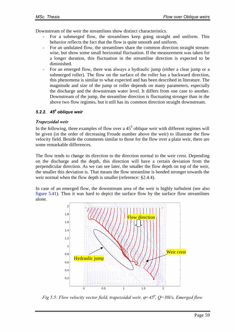
MSc. Thesis Flow over Oblique weirs
Page 59
Downstream of the weir the streamlines show distinct characteristics.- For a submerged flow, the streamlines keep going straight and uniform. This
behavior reflects the fact that the flow is quite smooth and uniform.- For an undulated flow, the streamlines share the common direction straight stream-
wise, but show some small horizontal fluctuation. If the measurement was taken fora longer duration, this fluctuation in the streamline direction is expected to bediminished.
- For an emerged flow, there was always a hydraulic jump (either a clear jump or asubmerged roller). The flow on the surface of the roller has a backward direction,this phenomena is similar to what expected and has been described in literature. Themagnitude and size of the jump or roller depends on many parameters, especiallythe discharge and the downstream water level. It differs from one case to another.Downstream of the jump, the streamline direction is fluctuating stronger than in theabove two flow regimes, but it still has its common direction straight downstream.
5.2.2. 450 oblique weir
Trapezoidal weirIn the following, three examples of flow over a 450 oblique weir with different regimes willbe given (in the order of decreasing Froude number above the weir) to illustrate the flowvelocity field. Beside the comments similar to those for the flow over a plain weir, there aresome remarkable differences.
The flow tends to change its direction to the direction normal to the weir crest. Dependingon the discharge and the depth, this direction will have a certain deviation from theperpendicular direction. As we can see later, the smaller the flow depth on top of the weir,the smaller this deviation is. That means the flow streamline is bended stronger towards theweir normal when the flow depth is smaller (reference: §2.4.4).
In case of an emerged flow, the downstream area of the weir is highly turbulent (see alsofigure 5.41). Thus it was hard to depict the surface flow by the surface flow streamlinesalone.
0 0.5 1 1.5 2
0.2
0.4
0.6
0.8
1
1.2
1.4
1.6
1.8
2
Fig 5.5: Flow velocity vector field, trapezoidal weir, =450, Q=30l/s, Emerged flow
Weir crest
Flow direction
Hydraulic jump
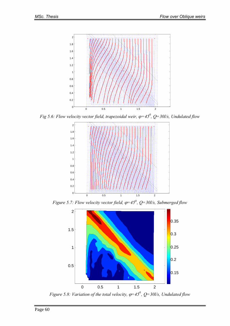
MSc. Thesis Flow over Oblique weirs
Page 60
0 0.5 1 1.5 20
0.2
0.4
0.6
0.8
1
1.2
1.4
1.6
1.8
2
Fig 5.6: Flow velocity vector field, trapezoidal weir, =450, Q=30l/s, Undulated flow
0 0.5 1 1.5 20
0.2
0.4
0.6
0.8
1
1.2
1.4
1.6
1.8
2
Figure 5.7: Flow velocity vector field, =450 , Q=30l/s, Submerged flow
0 0.5 1 1.5 2
0.5
1
1.5
2
0.15
0.2
0.25
0.3
0.35
Figure 5.8: Variation of the total velocity, =450 , Q=30l/s, Undulated flow

MSc. Thesis Flow over Oblique weirs
Page 61
Figure 5.8 and 5.6 come from the same test with a 450 weir, Q=30l/s and undulated flow.
The pattern of the flow velocity field and the weir geometry are well matched. It is shownthat the flow accelerates when it reaches the weir and decelerates when it leaves the weir.Contour lines are more or less parallel to the weir crest in the upstream part to the areaabove the weir. Only in the downstream region of the weir, the contour lines show a lessstructured characteristic.
When reaching the weir, the flow streamlines are bended to the right, and the flow isconverged to the right hand side of the flume. That causes a much higher velocity near theright side wall than the average velocity. To the left end of the weir, the flow also increaseits velocity due to a small separation zone near the weir crest. These higher velocities canbe observed in figure 5.8. This phenomenon is only an effect of the side wall, not anintrinsic property of the flow over an oblique weir.
Sharp-crested weirThe flow over a 450 oblique sharp-crested weir can be illustrated by the following figuresfrom experiment
(a) Emerged flow (b) Undulated flow
(c) Submerged flowFig 5.9: Flow velocity field for sharp crested weir, =450, Q=35l/s
The flow over this weir shows stronger bended streamlines than in the case of the 450
oblique trapezoidal weir. This means the deviation angle of the streamlines from thedirection normal to the weir crest is smaller. The asterisk point (*) denotes the center of theweir crest.

MSc. Thesis Flow over Oblique weirs
Page 62
0 100 200 300 400 500-0.1
0
0.1
0.2
0.3
0.4
0.5
0.6
Distance along the streamline
Ve
loci
ty(m
/s)
U (m/s)V (m/s)Total velocity (m/s)
(a) Sharp-crested weir (b) Trapezoidal weir
Fig 5.10: Velocity along the middle streamline, =450, Q=35l/s, undulated flow
Figure 5.10 illustrates the flow over two different type of weir (with the same oblique angle=450) under the same flow condition: undulated flow, Q=35l/s. It can be seen that theundulation (the waves) behind the sharp crested weir is much more pronounced than that inthe case of a trapezoidal weir. This is caused by the abrupt change in the sharp crested weirgeometry (an abrupt widening) in comparison with the gentle downstream slope of thetrapezoidal weir. The recirculation zone behind the sharp crested weir is much moredominant than that behind the trapezoidal weir because of the same reason.
Broad-crested weirThe broad crested weir has a long horizontal crest (relatively to the weir height) and abruptchanges in the weir geometry like the sharp crested weir, thus the flow over this weir sharesome similar characteristics with the two types of oblique weir mentioned above.
For the same flow condition, the deviation of the streamlines from the expected direction(normal to the weir crest) in is somewhat bigger than that in case of a sharp-crested weirand smaller than that of a trapezoidal weir, as will be shown in §5.5.
(a) Emerged flow (b) Undulated flow
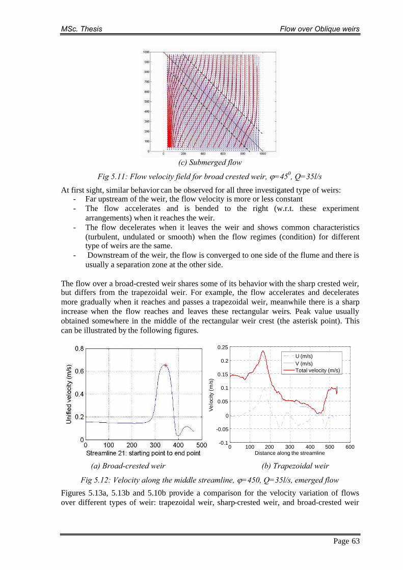
MSc. Thesis Flow over Oblique weirs
Page 63
(c) Submerged flow
Fig 5.11: Flow velocity field for broad crested weir, =450, Q=35l/s
At first sight, similar behavior can be observed for all three investigated type of weirs:- Far upstream of the weir, the flow velocity is more or less constant- The flow accelerates and is bended to the right (w.r.t. these experiment
arrangements) when it reaches the weir.- The flow decelerates when it leaves the weir and shows common characteristics
(turbulent, undulated or smooth) when the flow regimes (condition) for differenttype of weirs are the same.
- Downstream of the weir, the flow is converged to one side of the flume and there isusually a separation zone at the other side.
The flow over a broad-crested weir shares some of its behavior with the sharp crested weir,but differs from the trapezoidal weir. For example, the flow accelerates and deceleratesmore gradually when it reaches and passes a trapezoidal weir, meanwhile there is a sharpincrease when the flow reaches and leaves these rectangular weirs. Peak value usuallyobtained somewhere in the middle of the rectangular weir crest (the asterisk point). Thiscan be illustrated by the following figures.
0 100 200 300 400 500 600-0.1
-0.05
0
0.05
0.1
0.15
0.2
0.25
Distance along the streamline
Ve
loci
ty(m
/s)
VELOCITY VARIATION ALONG STREAMLINE 13. 45 Degrees, Q=35l/s, Emerged flow
U (m/s)V (m/s)Total velocity (m/s)
(a) Broad-crested weir (b) Trapezoidal weir
Fig 5.12: Velocity along the middle streamline, =450, Q=35l/s, emerged flow
Figures 5.13a, 5.13b and 5.10b provide a comparison for the velocity variation of flowsover different types of weir: trapezoidal weir, sharp-crested weir, and broad-crested weir
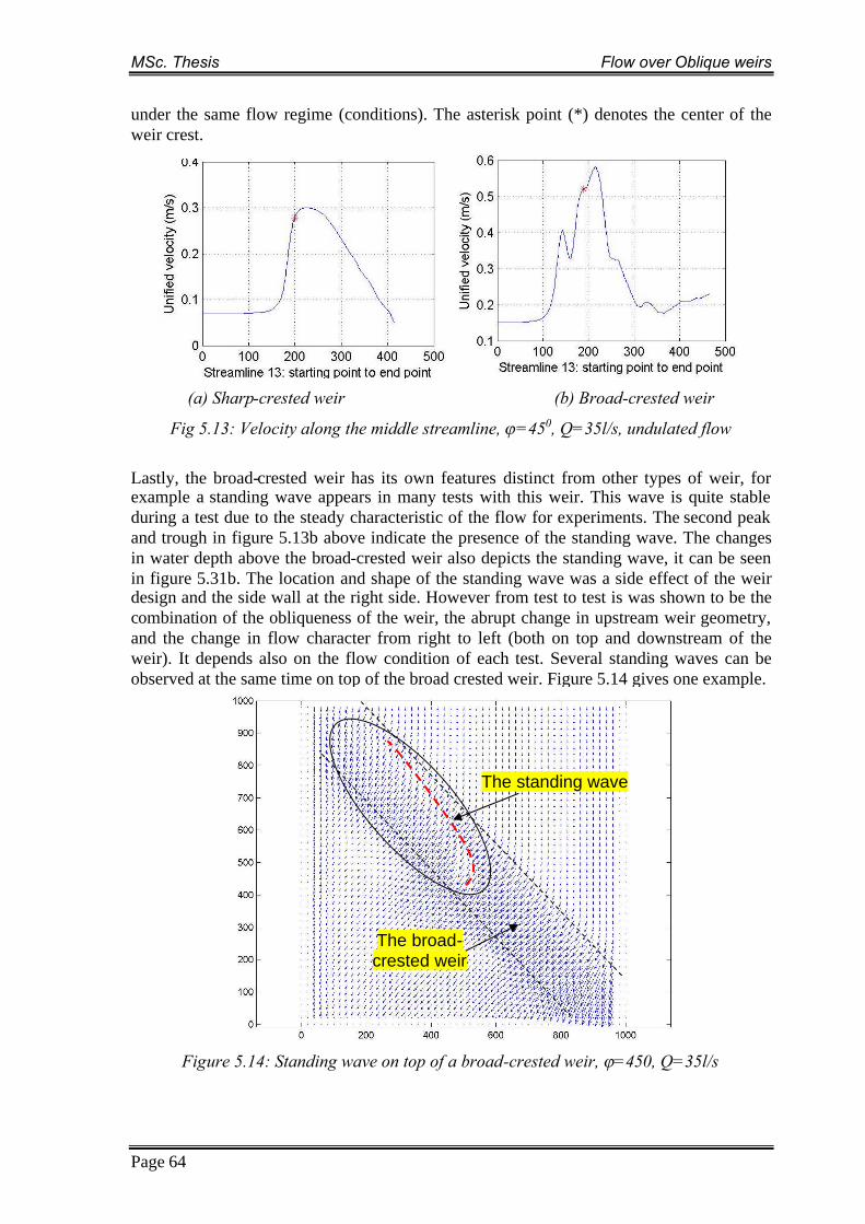
MSc. Thesis Flow over Oblique weirs
Page 64
under the same flow regime (conditions). The asterisk point (*) denotes the center of theweir crest.
(a) Sharp-crested weir (b) Broad-crested weir
Fig 5.13: Velocity along the middle streamline, =450, Q=35l/s, undulated flow
Lastly, the broad-crested weir has its own features distinct from other types of weir, forexample a standing wave appears in many tests with this weir. This wave is quite stableduring a test due to the steady characteristic of the flow for experiments. The second peakand trough in figure 5.13b above indicate the presence of the standing wave. The changesin water depth above the broad-crested weir also depicts the standing wave, it can be seenin figure 5.31b. The location and shape of the standing wave was a side effect of the weirdesign and the side wall at the right side. However from test to test is was shown to be thecombination of the obliqueness of the weir, the abrupt change in upstream weir geometry,and the change in flow character from right to left (both on top and downstream of theweir). It depends also on the flow condition of each test. Several standing waves can beobserved at the same time on top of the broad crested weir. Figure 5.14 gives one example.
Figure 5.14: Standing wave on top of a broad-crested weir, =450, Q=35l/s
The broad-crested weir
The standing wave

MSc. Thesis Flow over Oblique weirs
Page 65
5.2.3. 600 oblique weirThe three examples below illustrate the surface flow velocity vector field for three differentflow regimes. These figures do not cover the whole length of the oblique weir, but revealsome remarkable phenomena and the general trend of the flow over the 600 oblique weir.From the analysis of the surface velocity field alone, some differences with the flow overthe 450 oblique weir can be found:
- The deviation of the streamlines above the weir to the normal direction of the weiris bigger than that in the case of=450.
- There is a clear spiral movement downstream of the weir in the case of an emergedflow. Water particles inside the whirl take part in two movements at the same time:rolling movement in the direction of the submerge roller; and moving from right toleft of the weir while rolling.
0 0.5 1 1.5 20
0.2
0.4
0.6
0.8
1
1.2
1.4
1.6
1.8
2
Figure 5.15: Flow velocity vector field, =600, Q=40l/s, Emerged flow
0 0.5 1 1.5 2 2.5
0.2
0.4
0.6
0.8
1
1.2
1.4
1.6
1.8
2
Figure 5.16: Flow velocity vector field, =600, Q=35l/s, Undulating flow
Weir crest
Flow direction
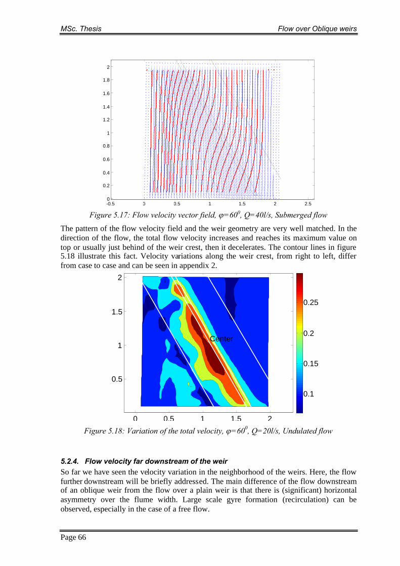
MSc. Thesis Flow over Oblique weirs
Page 66
-0.5 0 0.5 1 1.5 2 2.50
0.2
0.4
0.6
0.8
1
1.2
1.4
1.6
1.8
2
Figure 5.17: Flow velocity vector field, =600, Q=40l/s, Submerged flow
The pattern of the flow velocity field and the weir geometry are very well matched. In thedirection of the flow, the total flow velocity increases and reaches its maximum value ontop or usually just behind of the weir crest, then it decelerates. The contour lines in figure5.18 illustrate this fact. Velocity variations along the weir crest, from right to left, differfrom case to case and can be seen in appendix 2.
Center
0 0.5 1 1.5 2
0.5
1
1.5
2
0.1
0.15
0.2
0.25
Figure 5.18: Variation of the total velocity, =600, Q=20l/s, Undulated flow
5.2.4. Flow velocity far downstream of the weirSo far we have seen the velocity variation in the neighborhood of the weirs. Here, the flowfurther downstream will be briefly addressed. The main difference of the flow downstreamof an oblique weir from the flow over a plain weir is that there is (significant) horizontalasymmetry over the flume width. Large scale gyre formation (recirculation) can beobserved, especially in the case of a free flow.

MSc. Thesis Flow over Oblique weirs
Page 67
Emerged flowThe flow downstream of the 450 oblique weir with Q = 30l/s, emerged regime can beillustrated by the following figure.
0 0.5 1 1.5 2 2.5
0.2
0.4
0.6
0.8
1
1.2
1.4
1.6
1.8
2
FLOW VELOCITY FIELD WITH STREAMLINES. DOWNSTREAM OF WEIR, Q=30l/s, EMERGED FLOW
Figure 5.19: Downstream flow velocity vector field, =450, Q=30l/s, emerged flow
The above presented velocity field can be compared tothe flow in the picture below. In the picture, the flowdownstream of the weir show two clear zones with aboundary line (boundary band) represented by a largenumber of black tracers. Please keep in mind thedifferent in direction of the above figure and the picture.This picture was taken while the camera was looking inthe downstream direction; whereas the flow in figure5.19 is from top down.
Between the tracer band and the left side wall is the largescale gyre formation. Inside the gyre, the particles movein the anti-clockwise direction (figure 5.19).
Figure 5.20: Downstream flow separation, =450,emerged flow
The horizontal asymmetry can be visualized by plotting the flow velocity components on tographs. The two figures below show the decrease of the velocity from right to left of theflume at two cross sections:
- 5.21a: 1.5m downstream from the weir center; i.e. the cross section at the distanceof 1.5m from the bottom of figure 5.19.
- 5.21b: 2.5m downstream from the weir center; i.e. the cross section at the distanceof 0.5m from the bottom of figure 5.19, through the gyre center.
weir
Flow
Flow
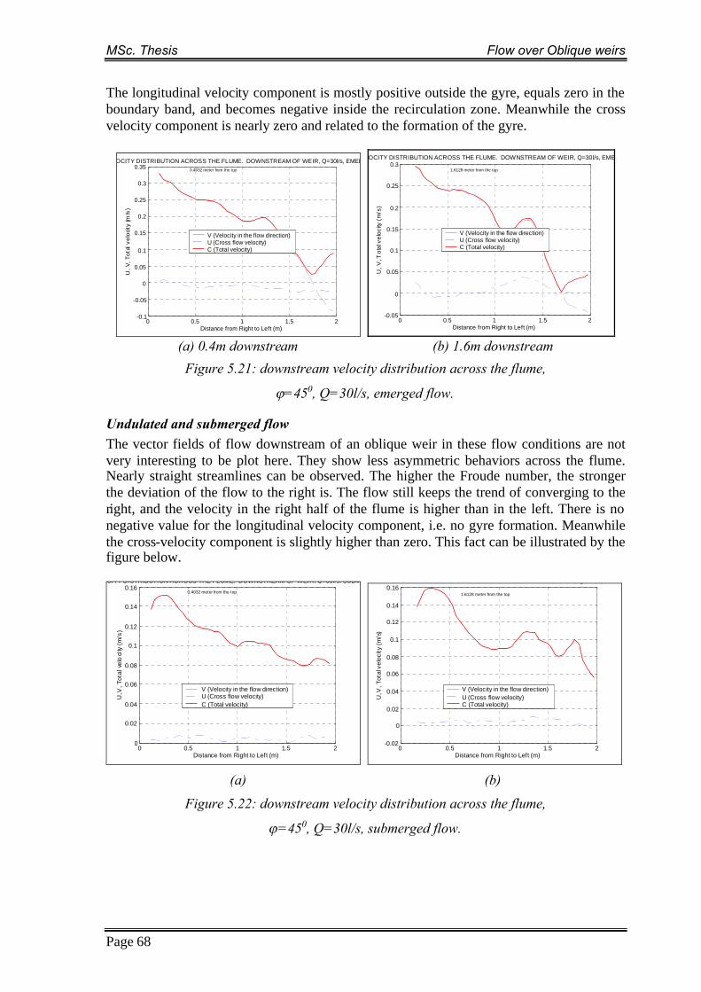
MSc. Thesis Flow over Oblique weirs
Page 68
The longitudinal velocity component is mostly positive outside the gyre, equals zero in theboundary band, and becomes negative inside the recirculation zone. Meanwhile the crossvelocity component is nearly zero and related to the formation of the gyre.
0 0.5 1 1.5 2-0.1
-0.05
0
0.05
0.1
0.15
0.2
0.25
0.3
0.35
Distance from Right to Left (m)
U,V
,Tot
alve
locit
y(m
/s)
FLOW VELOCITY DISTRIBUTION ACROSS THE FLUME. DOWNSTREAM OF WEIR, Q=30l/s, EMERGED FLOW0.4032 meter from the top
V (Velocity in the flow direction)U (Cross flow velocity)C (Total velocity)
0 0.5 1 1.5 2-0.05
0
0.05
0.1
0.15
0.2
0.25
0.3
Distance from Right to Left (m)
U,V
,Tot
alve
loci
ty(m
/s)
FLOW VELOCITY DISTRIBUTION ACROSS THE FLUME. DOWNSTREAM OF WEIR, Q=30l/s, EMERGED FLOW
1.6128 meter from the top
V (Velocity in the flow direction)U (Cross flow velocity)C (Total velocity)
(a) 0.4m downstream (b) 1.6m downstream
Figure 5.21: downstream velocity distribution across the flume,
=450, Q=30l/s, emerged flow.
Undulated and submerged flowThe vector fields of flow downstream of an oblique weir in these flow conditions are notvery interesting to be plot here. They show less asymmetric behaviors across the flume.Nearly straight streamlines can be observed. The higher the Froude number, the strongerthe deviation of the flow to the right is. The flow still keeps the trend of converging to theright, and the velocity in the right half of the flume is higher than in the left. There is nonegative value for the longitudinal velocity component, i.e. no gyre formation. Meanwhilethe cross-velocity component is slightly higher than zero. This fact can be illustrated by thefigure below.
0 0.5 1 1.5 20
0.02
0.04
0.06
0.08
0.1
0.12
0.14
0.16
Distance from Right to Left (m)
U,V
,Tot
alve
loci
ty(m
/s)
FLOW VELOCITY DISTRIBUTION ACROSS THE FLUME. DOWNSTREAM OF WEIR, Q=30l/s, SUBMERGED FLOW
0.4032 meter from the top
V (Velocity in the flow direction)U (Cross flow velocity)C (Total velocity)
0 0.5 1 1.5 2-0.02
0
0.02
0.04
0.06
0.08
0.1
0.12
0.14
0.16
Distance from Right to Left (m)
U,V
,Tot
alve
loci
ty(m
/s)
FLOW VELOCITY DISTRIBUTION ACROSS THE FLUME. DOWNSTREAM OF WEIR, Q=30l/s, SUBMERGED FLOW
1.6128 meter from the top
V (Velocity in the flow direction)U (Cross flow velocity)C (Total velocity)
(a) (b)
Figure 5.22: downstream velocity distribution across the flume,
=450, Q=30l/s, submerged flow.

MSc. Thesis Flow over Oblique weirs
Page 69
5.3. Vertical profiles of velocities
The velocity distribution over the flow depth is important to interpret its three dimensionalstructure. An insight into the intrinsic properties of the flow over an oblique weir and manyimportant conclusions can be obtained by investigating the vertical velocity profiles.
The vertical velocity profile was measured for some specific cases to illustrate the variationof velocity along the flow as well as to provide a glance on the velocity variation overchannel depth. Another phenomenon of interest investigated in this part of the thesis, is the(vertical) recirculation zone just behind the weir. The definition of coordinates in section3.5 is applied here.
5.3.1. Illustration of velocity profiles over flow depthTo illustrate the velocity variation along the flow, three measurements (with free flow,submerged flow and flow at transition state) were performed with each different weir’soblique angle. Below, typical velocity profiles over the depth in a steady open channel floware shown. This is two examples at one meter upstream of the weir and oblique weir in thecase of an emerged flow and submerged flow.
(a) Emerged flow (b) Submerged flow
Figure 5.23: Velocity distribution over the flow depth
The velocity distribution has a logarithmic profile, i.e. U ~ ln(z). Generally this relation isexpressed in the form of the following equation:
Czu
uU
*
*
ln1
(5.1)
or after small modification
**
* ln1
)ln(u
Cuzu
U (5.2)
where z : the elevation of the measurement pointU : flow velocity at elevation zu* : the shear stress velocity: Von Karman constant, = 0.401: kinematic viscosity, = 1.01. 10-6
C : constant, to be determined by experiments.
-105 -100 -95 -90 -85
0
2
4
6
8
10
12
14
16
18
20
ADV MEASUREMENT
Distance (cm)
Dep
th(c
m)
-104 -102 -100 -98 -96 -94 -92 -90 -88
0
2
4
6
8
10
12
14
ADV MEASUREMENT
Distance (cm)
Dep
th(c
m)

MSc. Thesis Flow over Oblique weirs
Page 70
The velocity is zero at the bottom of the flume, and increases over the depth.Measurements provide values of z and U for determining other parameters. Following isone example from velocity measurement one meter upstream of the weir. The flow velocitywas plotted against the flow depth (5.24a) and against the natural logarithm of the flowdepth (5.24b).
0
2
4
6
8
10
12
14
16
18
20
0.00 0.02 0.04 0.06 0.08 0.10 0.12
Velocity (m /s)
De
pth
(cm
)
Velocity
U ~ ln(z)
y = 0.012x + 0.1334
0.00
0.02
0.04
0.06
0.08
0.10
0.12
-6.0 -5.0 -4.0 -3.0 -2.0 -1.0 0.0
ln (z)
U(m
/s)
U ~ ln(z)
Linear (U ~ ln(z))
(a) (b)Figure 5.24: Relation between U and z
From these measurement points, the terms
*uand
*
* ln1 u
Cu can be determined.
Thus the value of u* and C can be calculated. Knowing u*, the friction slope can becalculated by:
gRu
S f
2* (5.3)
where R is the hydraulic radius of the flume, R = (B.d)/(B+2d), B is the flume width and dis the flow depth. The friction slope can be used to estimate the loss over a certain distancein the (free) flume by the flow resistance to use for simple flow models.
5.3.2. Velocity measurement along the flumePoint measurements were taken by an ADV at several positions (points) on the plan view(either along the center line of the flume or along the center streamline of the flow). Eachposition comprises of a number of points from bottom to surface. Due to the restriction inpositioning of the instrument, above the weir and close to the surface the ADV couldn’twork. Results from additional PTV analyses gave us the necessary information of thesurface flow velocity, which were used to compensate for this shortcoming.
The area of measurement was usually six meters, from two meter upstream to four metersdownstream of the weir. PTV analysis was expanded (when necessary) to cover this rangein order to provide enough information on the value of the surface velocity.
Following is one example from the experiment with = 600, Q = 40l/s, undulated flow.The measurement elaboration has been presented in chapter 3.5:
- Step1: Positioning measurement points for ADV (see figure 5.25).- Step 2: Determining surface flow velocity at those points by pre-analyses with
PTV.- Step 3: Measuring at each position: from bottom to 5cm below the free surface.- Step 4: Processing the data from ADV measurements and export to figures.

MSc. Thesis Flow over Oblique weirs
Page 71
The procedure and results are presented below. Some other flow profiles for different flowregimes can be seen in appendix 3.
Figure 5.25: Positioning the measurement points
The surface velocities (results from three PTV analyses) are plotted on the following graph:
0
0.05
0.1
0.15
0.2
0.25
0.3
0.35
0.4
0.45
-3 -2 -1 0 1 2 3
X (m)
Tot
alv
elo
city
(m/s
)
Total velocity
Figure 5.26: Surface flow velocity along the center streamline
Results from PTV and ADV data analysis for this experiment and its measurementpositions can be summarized in the following table:
Table 5.1: Measurements of velocity profiles
Measurement positions
Y X Bottom Depth Surface
Totalvelocity at
surface
StreamlineAngle
V atsurface
Depthaveraged
velo.TestNo.
(cm) (cm) (cm) (cm) (cm) (m/s) (0) (m/s) (m/s)
1 20 -200 0 14.18 14.18 0.179 0.0 0.179 0.132
2 20 -100 0 14.45 14.45 0.194 0.0 0.194 0.1393 16 -40 2.22 11.72 13.94 0.202 21.7 0.188 0.0004 0 0 10.4 3.15 13.55 0.291 26.3 0.260 0.0005 -12 20 5.46 8.09 13.55 0.394 30.1 0.341 0.1346 -18 30 2.7 10.69 13.39 0.343 33.1 0.287 0.1157 -25 40 0 13.61 13.61 0.306 25.6 0.276 0.1358 -30 60 0 14.03 14.03 0.239 14.0 0.232 0.1389 -35 80 0 14.16 14.16 0.225 14.0 0.218 0.142
10 -40 100 0 14.24 14.24 0.194 7.5 0.193 0.14211 -42 200 0 14.26 14.26 0.162 3.2 0.162 0.13512 -50 400 0 14.28 14.28 0.143 5.2 0.142 0.127
The center streamline
Measurement points
Flow direction
weir
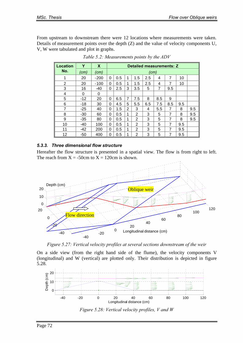
MSc. Thesis Flow over Oblique weirs
Page 72
From upstream to downstream there were 12 locations where measurements were taken.Details of measurement points over the depth (Z) and the value of velocity components U,V, W were tabulated and plot in graphs.
Table 5.2: Measurements points by the ADV
Y X Detailed measurements: ZLocationNo. (cm) (cm) (cm)1 20 -200 0 0.5 1 1.5 2.5 4 7 102 20 -100 0 0.5 1 1.5 2.5 4 7 103 16 -40 0 2.5 3 3.5 5 7 9.54 0 05 -12 20 0 6.5 7 7.5 8 8.5 96 -18 30 0 4.5 5 5.5 6.5 7.5 8.5 9.57 -25 40 0 1.5 2 3 4 5.5 7 8 9.58 -30 60 0 0.5 1 2 3 5 7 8 9.59 -35 80 0 0.5 1 2 3 5 7 8 9.5
10 -40 100 0 0.5 1 2 3 5 7 9.511 -42 200 0 0.5 1 2 3 5 7 9.512 -50 400 0 0.5 1 2 3 5 7 9.5
5.3.3. Three dimensional flow structureHereafter the flow structure is presented in a spatial view. The flow is from right to left.The reach from X = -50cm to X = 120cm is shown.
-40-20
020
4060
80100
120
-40
-20
0
20
0
10
20
Longitudinal distance (cm)
Depth (cm)
Figure 5.27: Vertical velocity profiles at several sections downstream of the weir
On a side view (from the right hand side of the flume), the velocity components V(longitudinal) and W (vertical) are plotted only. Their distribution is depicted in figure5.28.
-40 -20 0 20 40 60 80 100 120
0
10
20
ADV MEASUREMENT
Longitudinal distance (cm)
Dep
th(c
m)
Figure 5.28: Vertical velocity profiles, V and W
Flow direction
Oblique weir

MSc. Thesis Flow over Oblique weirs
Page 73
5.3.4. Analysis of the flow structure
GeneralBy looking at the velocity distribution along the middle streamline of the flow (more orless in the middle part of the flume), the unwanted effects of the side walls had beenavoided. Because this procedure of analysis is time consuming, usually only one streamlineis investigated for each weir configuration and flow regimes. Anyhow by using this singleexample, it is possible to acquire a relatively general understanding about the whole flow.
Generally speaking, the flow structure in the neighborhood of an oblique weir is far morecomplicated from two dimensional with various complex phenomena. Far away from theoblique weir, the across asymmetry is diminished and the flow structure returns to itstypical and well known structure of the flow in an (shallow) open channel flow. This is alsotrue for the flow region far upstream of the weir.
Depending on the flow regimes, the flow structure can be essentially different. The aboveexample is a representation for the submerged flow or the surface-jet flow, and theundulated flow. For such flow regimes, in the region just behind the weir the flow isstrongly twisted. The straight and flat cross section along one straight streamline in the caseof a perpendicular weir now turns to a curved and twisted surface. The surface velocity isbigger and bias to the right, while going down to the bottom, the velocity graduallydecrease and turn its direction to the left. The difference in sub-layers of the flow can beillustrated by the following figure. The viewing direction in the figure is looking upstream.
-40
-20
0
20
40
60
80
100
120-50 -40 -30 -20 -10 0 10 20
0
10
20
Longitudinal distance (cm)
Depth (cm)
Figure 5.29: Velocity variations along the streamline and over the depth.
Longitudinal and vertical velocity componentsFar upstream and downstream of the weir, the flow velocity profile has the typicaldistribution which has been discussed in section 5.3.1. Hereafter only the velocity profilesin the region behind the weir are presented. They show a combination of a flow in an openchannel (in the lower part) and a surface jet-flow (in the upper part).

MSc. Thesis Flow over Oblique weirs
Page 74
Figure 5.30: Velocity profiles on the downstream and on the slope of the weir.
The high velocity layer is above the weir crest, while the velocity in the lower layerdevelops from the bottom in a logarithmic profile. The mixing layer between the two has aslightly lower longitudinal velocity component. This difference tends to smoothen out faraway from the weir.
The vertical velocity component is varied depending on the measurement location. On thedownstream slope of the weir, it is in agreement with the change in weir geometry. Furtherdownstream it shows some small fluctuations around the value of zero.
Across flume velocity componentTheoretically there is no significant transfer of water mass across the flume in the case of aflow over a perpendicular weir. With an oblique weir the situation is far different; there isalways mass transfer across the flume in the neighborhood of the weir. Upstream andabove the weir, the flow is converged to the right, thus the water depth here is usuallyhigher than that on top of the weir crest in the left part (see also next part).
To see the variation of this velocity component in the downstream neighborhood of theweir, we consider an example as shown in figure 5.27 and 5.29. If the flow in this examplecan be divided into sub-layers, then the flow in the upper layers mostly turn to the right,meanwhile the lower layers mostly turn to the left, or at least their direction is kept straight.Things were different for an emerged flow, where the upper velocity mostly turns to theleft and the lower velocity turns to the right (see fig.5.15; fig.2.16). Thus the water mass isalways exchanged between left and right parts across the flume, associated to its velocity.
Differences in water level above the weir crestAs mentioned before, the water level on top of the weir crest always have some smallchanges. It decreases from right to left. The difference (H) is depending on the Froudenumber above the weir and can be as big as 5mm (10% of the water depth on top of theweir).
1.5
1.7
1.9
2.1
2.3
2.5
2.7
2.9
3.1
0 0.5 1 1.5
Weir crest (cm)
Dep
th(c
m)
Right
Center
Left
-3
-2
-1
0
1
2
3
4
5
0 10 20 30 40 50
Distance (cm)
Wat
er
dep
th(c
m)
Right
Center
Undisturbed
Left
(5.31a) Sharp-crested weir, Q=35l/s (5.31b) Broad-crested weir, Q=35l/sFigure 5.31: Water level variation above the weir in stream-wise direction
Free surface

MSc. Thesis Flow over Oblique weirs
Page 75
0.00
0.02
0.04
0.06
0.08
0.10
0.12
0.0 0.1 0.2 0.3 0.4 0.5 0.6
Fr1
DH
/H1
Series1
(c) Trapezoidal weir: the relative loss and Fr1Figure 5.32: The left-right difference in water depth above the weir
Data plotted on figure 5.31 was taken from many tests with different discharge. Therelative loss was calculated by first calculating the absolute loss from the water depth at themiddle point of the weir crest from right to left:
H = h1right – h1left (5.4)
5.3.5. The recirculation zone
When we change the oblique angle of the weir, a remarkable phenomenon was observed inthe study of Wols. The recirculation zone behind the weir in case of oblique angle equals600 is more evident than that in case of 450 and 300 . With a perpendicular weir, therecirculation zone was hardly observed. Inside the recirculation zone, the flow has partly abackward velocity. It is expected that the direction of the whirl movement inside therecirculation zone is opposite to that inside a hydraulic jump. There is a hydraulic jumpbehind weir in the case of emerged flow, and there is almost no recirculation movement inthe case of an entirely submerged flow. The size of the recirculation zone is usually clearestwhen the flow is in a transitional state, which is the flow with undulation behind weir.
Because of left-right asymmetry in the area adjacent to the weir, there the recirculationzone differs from left to right. It has a stronger backward velocity on the left hand side(stream wise direction), where the flow state is closer to the submerged state, and a weakerbackward velocity on the right hand side, where the flow closer to the emerged state. Thisis due to the increase of the flow depth along the weir crest from left to right, which makesthe H1/H2 ratio increased.
Detailed measurements were taken with the 600 oblique weir. But as a matter of fact, therecirculation zone wasn’t found. As can be seen in figure 5.28, there is no backwardvelocity for the longitudinal component in the downstream part of the weir. The flowstructure is not disturbed too much because of the gentle and quite smooth change in weirgeometry. This is different from result of Wols’ simulations. One of his examples is shownhere below:
Figure 5.33: The recirculation zone behind a trapezoidal weir, q=0.15m2/s

MSc. Thesis Flow over Oblique weirs
Page 76
As we can see, the difference in figure 5.28 (experiment) and figure 5.32 (simulation) isquite significant. The recirculation zone in the result of simulations is quite pronounced;while there is no recirculation zone in the results of the experiments. One of the reasons forthis difference is the much higher specific discharge (q = 0.15m2/s for this simulation run)used in his simulation in comparison with the specific discharge range in our experiments(q = 0.005 0.01m2/s), i.e. a much higher velocity, whereas the order of the water depth isof the same (h1, h2 is in the order of 0.2m). The Reynolds number may play a role in thisdifference, as the experiment has a much lower Re number than the simulation has.
It is understandable that the more abrupt the downstream weir geometry is, the strongerrecirculation behavior can be found. The old experiments on sharp-crested and broad-crested rectangular weirs always show bigger recirculation zone in comparison withtrapezoidal weirs. The spiral movement behind an oblique rectangular weir (clockwise,from right to left of the flume along the downstream edge of the oblique weir) can be easierobserved. The following example is a simulation with the same dimensions andarrangement of the real sharp-crested weir in the flume (result from B.A. Wols). Therecirculation zone can be seen much more prominent.
Figure 5.34: The recirculation zone behind a sharp-crested weir, q=0.15m2/s
5.4. Two velocity component analysis
5.4.1. Velocity variation along the flow
The velocity component analysis has been presented in chapter 2. Hereafter some generaland remarkable results will be shown. This type of analysis was applied to the surfacevelocity and proved to be very useful during the course of this study.
Velocity variation and flow regimesThe velocity and its components (parallel and perpendicular to the weir) vary along theflow. This variation not only depends on the spatial position, but also the flow state andregimes. There three flow regimes can be distinguished. The comparison for them is shownbelow.
0 100 200 300 400 500-0.05
0
0.05
0.1
0.15
0.2
0.25
0.3
Distance along the streamline
Velo
city
(m/s
)
U (m/s)V (m/s)Total velocity (m/s)
0 50 100 150 200 250 300 350 400 450 500-0.1
-0.05
0
0.05
0.1
0.15
0.2
0.25
Distance along the streamline
Ve
loci
ty(m
/s)
VELOCITY VARIATION ALONG STREAMLINE 13. 45 Degrees, Q=40l/s, Emerged flow
U (m/s)V (m/s)Total velocity (m/s)
(5.34a) Emerged flow (5.34b) Emerged flow

MSc. Thesis Flow over Oblique weirs
Page 77
0 100 200 300 400 500-0.05
0
0.05
0.1
0.15
0.2
0.25
0.3
Distance along the streamline
Vel
oci
ty(m
/s)
VELOCITY VARIATION ALONG STREAMLINE 13. Q=25l/s, FLOW WITH UNDULATION
U (m/s)V (m/s)Total velocity (m/s)
0 100 200 300 400 500-0.02
0
0.02
0.04
0.06
0.08
0.1
0.12
0.14
0.16
0.18
Distance along the streamline
Vel
ocity
(m/s
)
U (m/s)V (m/s)Total velocity (m/s)
(5.34c) Undulated flow (5.34d) Submerged flow
Figure 5.34: Velocity components analysis for different flow regimes.
Figure 5.34a, c and d are typical variations along the streamlines of flow over an obliqueweir in the case of free flow, undulated flow and submerged flow respectively. Usually forthe emerged flow, the valid range of the velocity component analysis is only the first halfof the streamline. Figure 5.34b is the one experiment in which this analysis is valid over thewhole length of the streamline. The recovery of velocity behind the weir is found in thisexample (5.34b).
As can be seen in the figures, the variation of velocity (components) along one streamlineis close related to the flow regime. It increases and decreases relatively fast and sharply inthe case of an emerged flow, usually with a sharp peak in the chart. Flow velocities changemore gently with an undulated flow and much more gradually with a submerged flow. Thevelocity profile in the case of a submerged flow looks like an inverted profile of the changein depth, i.e. its shape is very much like the profile of the trapezoidal weir cross section,even though the downstream slope of the velocity profile is more moderate.
Velocity variation and weir geometryThe figures above illustrate the variation of velocity in the flow over a trapezoidal weir.Examples of the flow over oblique, sharp-crested (Q=15l/s, emerged flow) and broad-crestedweir (Q=35l/s, submerged flow) can be seen hereafter.
0
0.02
0.04
0.06
0.08
0.1
0.12
0.14
0.16
0.18
0 0.5 1 1.5 2Distance (m)
Velo
city
(m/s
)
VP
VL
Total Velocity
0
0.02
0.04
0.06
0.08
0.1
0.12
0.14
0 0.05 0.1 0.15 0.2
Distance (m)
Vel
oci
ty(m
/s)
VP
VL
Total Velocity
(a) Sharp-crested weir (b) Broad-crested weir
Figure 5.35: Velocity variation with different weir configurations

MSc. Thesis Flow over Oblique weirs
Page 78
Contribution of velocity componentsAnother remarkable fact is that the variation of the velocity component perpendicular to theweir contributes greatly to the variation of the total velocity, meanwhile the velocitycomponent parallel to the weir only play a lesser role. They both follow quite well the trendof variation in the total velocity profile. All the figures with velocity component ana
This fact strengthens the assumption that has been used for analytical research of the flowover an oblique weir (chapter 2). Many relations between flow variables could only befound by means of energy conservation and momentum conservation thanks to theassumption of constant velocity component parallel to the weir.
5.4.2. Velocity variation across the flowThe variation across the flume has been presented in section 5.2.4. Here after the velocityvariation along the weir crest (i.e. across the flume) will be briefly presented.
0 0.5 1 1.5 2 2.5 3 3.5 4-0.05
0
0.05
0.1
0.15
0.2
0.25
0.3
0.35
Distance (m)
Velo
city
(m/s
)
U (m/s)V (m/s)Total velocity (m/s)
0 0.5 1 1.5 2 2.5 3 3.5 40.02
0.04
0.06
0.08
0.1
0.12
0.14
0.16
0.18
Distance (m)
Velo
city
(m/s
)U (m/s)V (m/s)Total velocity (m/s)
(a) Trapezoidal weir, emerged flow (b) Trapezoidal weir, submerged flow
(c) Sharp-crested weir (d) Broad-crested weirFigure 5.36: Velocity variation along the weir crest
The variation along the weir crest also depends on the flow regimes. For example with asharp-crested weir, the velocity tends to increase from right to left with an emerged flow,meanwhile it shows an opposite trend in the case of a submerged flow.
5.4.3. Spatial (2D) variation of the velocity componentsThe velocity can be further analyzed for the whole field. From the chart describe thechange in total velocity, it can be seen very clear that the flow start to accelerate when it“feel” the change in bottom topography. Maximum velocity is observed at the crest of weirin all cases, followed by a deceleration zone. A typical view is shown below.
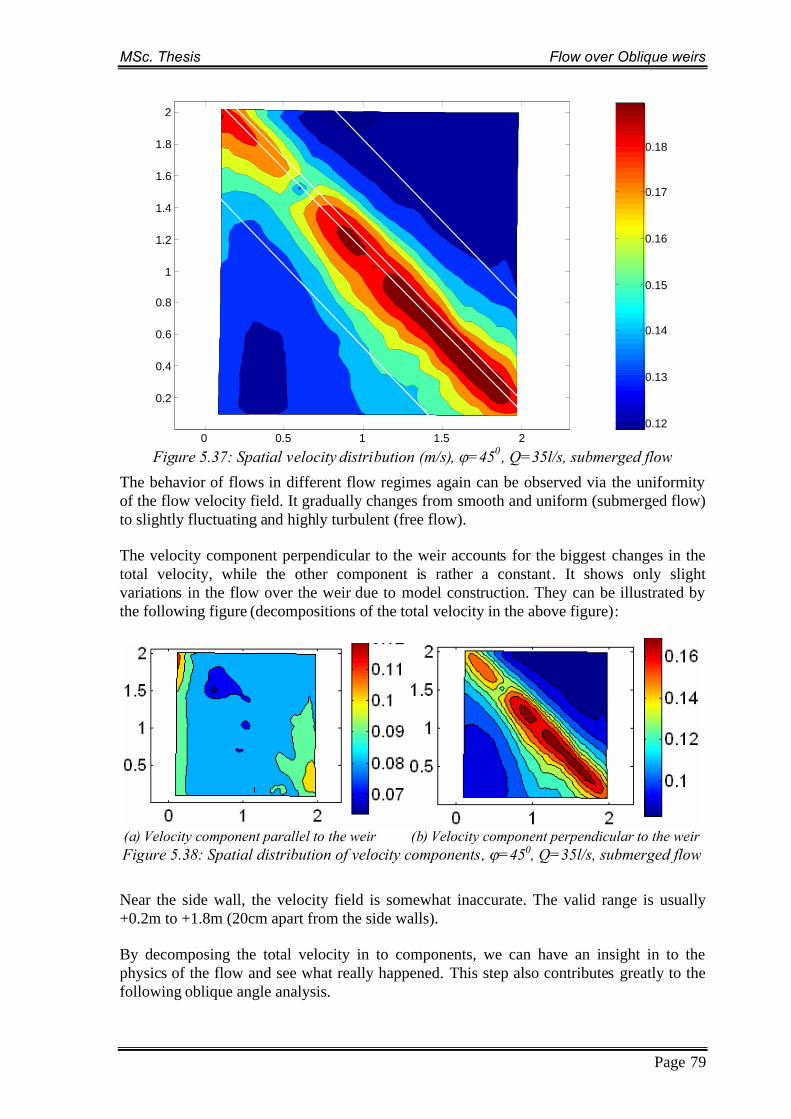
MSc. Thesis Flow over Oblique weirs
Page 79
Total Velocity
0 0.5 1 1.5 2
0.2
0.4
0.6
0.8
1
1.2
1.4
1.6
1.8
2
0.12
0.13
0.14
0.15
0.16
0.17
0.18
Figure 5.37: Spatial velocity distribution (m/s), =450 , Q=35l/s, submerged flow
The behavior of flows in different flow regimes again can be observed via the uniformityof the flow velocity field. It gradually changes from smooth and uniform (submerged flow)to slightly fluctuating and highly turbulent (free flow).
The velocity component perpendicular to the weir accounts for the biggest changes in thetotal velocity, while the other component is rather a constant. It shows only slightvariations in the flow over the weir due to model construction. They can be illustrated bythe following figure (decompositions of the total velocity in the above figure):
(a) Velocity component parallel to the weir (b) Velocity component perpendicular to the weirFigure 5.38: Spatial distribution of velocity components, =450, Q=35l/s, submerged flow
Near the side wall, the velocity field is somewhat inaccurate. The valid range is usually+0.2m to +1.8m (20cm apart from the side walls).
By decomposing the total velocity in to components, we can have an insight in to thephysics of the flow and see what really happened. This step also contributes greatly to thefollowing oblique angle analysis.

MSc. Thesis Flow over Oblique weirs
Page 80
5.5. Angle of obliqueness5.5.1. GeneralThe oblique angles in all experiments were plotted for the whole field to give an overviewof the changes in flow direction. The angle at some specific locations (in which the centerof the weir is the most important point) is given in number. They are also tabulated andplotted in graphs to show the trend of changing these angles.
0 0.5 1 1.5 20
0.2
0.4
0.6
0.8
1
1.2
1.4
1.6
1.8
2
Min Angle
Max Velocity
0 0
25
30
35
40
45
50
Figure 5.39: Spatial distribution of oblique angle, =450, Q=30l/s, submerged flow
The flow tends to change angle () closer to the direction perpendicular to the weir crestwhen the flow depth decreases. It also shows some non-uniform as the flow regimechanges from submerged to undulated and emerged (figure 5.40 and 5.41 respectively). Inthe emerged condition, the flow downstream of an oblique weir is highly turbulent andchaotic.
0 0.5 1 1.5 20
0.2
0.4
0.6
0.8
1
1.2
1.4
1.6
1.8
2
Min Angle
Max Velocity
15
20
25
30
35
40
Figure 5.40: Spatial distribution of oblique angle, =450, Q=30l/s, undulated flow

MSc. Thesis Flow over Oblique weirs
Page 81
0 0.5 1 1.5 2
0.2
0.4
0.6
0.8
1
1.2
1.4
1.6
1.8
2
Min Angle
Max Velocity
Oblique angle at center = 15.03550 Min angle = -44.34710
-40
-20
0
20
40
60
80
100
Figure 5.41: Chaos downstream of an oblique angle, =450, Q=30l/s, emerged flow
The visualization of the flow direction also reveals some phenomena that have beendiscussed earlier. For example when there is a clear roller behind the weir in case of anemerged flow, we can observe the recirculation zone and the spiral movement from right toleft in the downstream neighborhood of the weir. The figure below illustrates that for thecase of Q=40l/s, = 600 (emerged flow).
0 0.5 1 1.5 20
0.2
0.4
0.6
0.8
1
1.2
1.4
1.6
1.8
2
Center
Min Angle
Max Velocity
Oblique angle at center = 35.38630 Min angle = 30.09620
40
50
60
70
80
90
100
Figure 5.42: Spatial distribution of oblique angle, =600, Q=40l/s, emerged flow
Similar to the spatial distribution of the velocity, the spatial distribution of the obliqueangle and the weir geometry are well matched. This is understandable because the angle isrelated to the velocity as shown by the velocity component analysis (chapter 2).

MSc. Thesis Flow over Oblique weirs
Page 82
5.5.2. Oblique trapezoidal weir, = 450
Many PTV analyses and measurement were done to provide data for this analysis ofoblique angle alone. Their experimental conditions and some major results are shown in thefollowing table:
Table 5.3: Extra measurements for oblique angle, = 450
Q H0 H0/aw Fr0p H1 H1/aw U1 Fr1p Fr1p/Fr0p tan()/tan()
l/s (cm) - - (cm) - (m/s) PTV - ( 0) -
20 13.18 1.27 0.05 1.82 0.18 0.28 0.65 13.86 13.27 0.2420 13.28 1.28 0.05 2.20 0.21 0.33 0.70 14.91 9.83 0.1720 18.23 1.75 0.03 7.56 0.73 0.13 0.13 4.57 24.12 0.45
25 13.62 1.31 0.06 2.10 0.20 0.26 0.54 9.71 16.54 0.3025 14.23 1.37 0.05 3.31 0.26 0.26 0.44 8.30 14.59 0.2625 17.23 1.66 0.04 6.48 0.62 0.16 0.19 4.77 22.05 0.4130 14.02 1.35 0.06 2.30 0.22 0.35 0.70 10.90 15.04 0.27
30 14.41 1.39 0.06 3.33 0.32 0.36 0.61 9.85 15.65 0.2830 19.29 1.85 0.04 8.50 0.82 0.18 0.18 4.56 22.30 0.4135 14.40 1.38 0.07 2.31 0.22 0.19 0.36 5.04 23.51 0.4435 14.78 1.42 0.07 3.55 0.34 0.40 0.65 9.32 15.47 0.28
35 19.28 1.85 0.05 8.48 0.82 0.18 0.18 3.88 26.07 0.4940 14.75 1.42 0.08 2.92 0.28 0.22 0.37 4.63 24.57 0.4640 15.67 1.51 0.07 4.59 0.44 0.13 0.20 2.68
40 18.28 1.76 0.06 7.34 0.71 0.23 0.24 4.19 24.58 0.46
The agreement of the measurement data with the prediction from theoretical analysis isshown in the following figures.
0 0.05 0.1 0.15 0.20
10
20
30
40
h1
(m)
(
0 )
TheoryExperiments
0 0.2 0.4 0.6 0.8 10
10
20
30
40
Fr1
(0 )
TheoryExperiments
Figure 5.43: Result of oblique angle analysis for the 450 oblique weir
The agreement appears to be quite good, although there are some deviations from thetheoretical line at high Froude numbers. This fact strengthens the validity of theassumptions that have been made in the theory analysis step.
The measured data also fit with the trend of the relation line between tan/tanandFr1/Fr0. There is a gap between the absolute value of the measurement data and theexpected value. It looks like an offset from the theoretical line to the measurement points.The deviation angle () is somewhat bigger than expected, i.e. the streamlines are expectedto be stronger curved. This can be explained by the reason: the surface velocity from PTVanalysis has been used to calculate Fr1p instead of the mean velocity (depth averagedvelocity) above the weir (U1).

MSc. Thesis Flow over Oblique weirs
Page 83
0.0
0.2
0.4
0.6
0.8
1.0
1.2
0 5 10 15Fr1/Fr0
tanb
/tan
j
ExperimentsTheory
Figure 5.44: Relation among , and flow conditions.
5.5.3. Oblique trapezoidal weir, = 600
The result of oblique angle analysis for this weir is summarized as follow:
Table 5.4: Extra measurements for oblique angle, = 600
Q H0 H0/aw Fr0p H1 H1/aw U1 Fr1p Fr1p/Fr0p tan()/tan()
l/s (cm) - - (cm) - (m/s) PTV - ( 0) -20 12.85 1.24 0.03 1.44 0.14 0.37 0.96 27.71 12.00 0.1225 13.17 1.27 0.04 1.70 0.16 0.25 0.56 13.34 24.52 0.26
30 13.51 1.30 0.05 1.91 0.18 0.26 0.53 10.95 28.06 0.3135 13.83 1.33 0.05 2.15 0.21 0.33 0.67 12.32 22.23 0.2440 14.12 1.36 0.06 2.34 0.26 0.26 0.44 7.35 35.40 0.4140 16.37 1.57 0.05 5.48 0.53 0.26 0.30 6.25 31.82 0.36
40 15.43 1.48 0.05 4.45 0.43 0.29 0.37 7.11 29.78 0.3340 14.70 1.41 0.06 3.45 0.33 0.33 0.51 9.00 27.39 0.3040 14.39 1.38 0.06 2.85 0.27 0.37 0.63 10.84 25.97 0.2840 14.31 1.38 0.06 2.74 0.26 0.37 0.65 11.02 25.11 0.27
40 14.11 1.36 0.06 2.32 0.22 0.39 0.73 12.19 24.54 0.2640 18.97 1.82 0.04 8.07 0.78 0.19 0.15 3.96 43.60 0.5540 17.81 1.71 0.04 6.92 0.67 0.20 0.20 4.72 35.52 0.4140 16.86 1.62 0.05 5.92 0.57 0.24 0.27 5.86 31.73 0.36
40 16.39 1.58 0.05 5.42 0.52 0.26 0.28 5.89 37.06 0.4430 18.02 1.73 0.03 7.19 0.69 0.16 0.15 4.80 37.03 0.4430 16.67 1.60 0.04 5.80 0.56 0.18 0.20 5.65 34.60 0.40
0 0.05 0.1 0.15 0.20
10
20
30
40
50
h1 (m)
(0 )
TheoryExperiments
0 0.2 0.4 0.6 0.8 10
10
20
30
40
50
Fr1
(
0 )
TheoryExperiments
Figure 5.45: Result of oblique angle analysis for the 600 oblique weir

MSc. Thesis Flow over Oblique weirs
Page 84
Bigger deviations of the value of oblique angles are found in the region with high Froudenumber. For a submerged flow condition, when the Froude number is small, the theoreticalanalysis gives good predictions for the value of flow oblique angle.
Below, the relation among , and flow condition is presented in figure 5.46. Theexperiments with a weir with = 600 show results which are not as good as results fromthe case of = 450. The data from the measurements still follow the expected values quitewell, although there are some deviations from the theory line. Beside the reasonsmentioned earlier, this deviation could also be caused by the big value of in relation witha relative narrow flume. In this situation, the length of the oblique weir is more than fourmeters (including weir slopes); meanwhile the width of the conveyer flume is only twometers. This fact may cause the effects of the side wall become relatively large.
0.0
0.2
0.4
0.6
0.8
1.0
1.2
0 2 4 6 8 10 12 14Fr1/Fr0
tan
b/t
anj
Measurements 60
Theory
Measurement 45
Figure 5.46: Relation among , and flow conditions.
The theoretical lines for weir 45 and 600 were constructed based on energy conservationand continuity equations of the flow. For an infinitely shallow flow, this line will end up at00 for every oblique weir, i.e. the flow direction above the weir will perpendicular to thecrest. The measurement data for both oblique angles follows this line quite well.
It can be seen that the thinner the water layer on top of the weir is, the stronger thestreamlines are curved. The ultimate situation is that all the streamlines are perpendicular tothe weir crest (similar to what happens with a plain weir). That showed in the above figurewith the limit oftends to zero when h1 comes to zero.
At high Froude number (or low water depth, small h1) the deviation of measurement datafrom the theoretical line is somewhat stronger. This can be explained by taking intoaccount the fact that measurement of h1 cannot be perform properly for the tests with freeflow because the free surface is strongly curved, the streamlines is no more horizontal. Thisfact is also reflected in the following figure, which shows the experimental values of u1calculated from h1, against the theoretical values.

MSc. Thesis Flow over Oblique weirs
Page 85
CHAPTER 6. DISCUSSION
6.1. General structure and behavior of the flow
The experiments on oblique weirs were performed for both sharp-crested and broad-crestedweirs. The results presented in the above chapters show some general phenomena andsimilar behavior but also some differences.
For both types of oblique weirs, the flow always turns its direction towards a perpendicularorientation when it reaches and passes the weir. The flow over the oblique part of the weirmostly turns towards weir normal direction. The flow accelerates when it reaches the weirand decelerates when it leaves the weir. Maximum velocities can be observed above theweir crest for the case of a sharp crested weir. For the case of a broad crested weir, themaximum velocity was observed just behind the weir.
From one side of the flume to the other, there are many differences in flow characteristic.Downstream of the weir, the two side walls force the flow to its initial direction, thus theflow converges to one side of the flume and a separation zone can be observed on the otherside. In these experiments, where the oblique angle is 450 and the weir alignment is asmentioned before, the water level at the right hand side is higher than the water level at theleft side, whereas the flow velocity at the left side is usually higher than at the right.
Changing the downstream water level will lead to changes in the flow regime and thebehavior of the flow over the oblique weir. With low downstream water level, there isusually a classical hydraulic jump. The hydraulic jump is dominant at the right side of theflume. To the left, the flow has a smoother pattern. Increasing the downstream water levelfurther, the hydraulic jump will change into an undular jump.
The energy dissipation of both the oblique sharp-crested weir and the broad-crested weirhas its maximum value for the case of a hydraulic jump behind weir, and minimum valuefor the case of completely submerged flow.
The discharge coefficient of an oblique weir (both sharp-crested and broad crested weir,with oblique angle equals 450) is much higher than the discharge coefficient of aperpendicular weir with the same channel width and water depth. That implies a lowerwater head in front of an oblique weir than in front of a perpendicular weir when thechannel width and the discharge do not change.
With the sharp-crested weir, the magnitude of the total velocity C tends to increase fromthe right hand side of the flume to the left in the case of a free flow (perfect weir) and viceversa for the case of a submerged flow (imperfect weir).
With the broad crested weir, a noticeable standing wave on top of the weir crest appears inmost of the cases with low discharge and free flow conditions. The results fromexperiments also show that for a broad crested weir, in the case of submerged flow

MSc. Thesis Flow over Oblique weirs
Page 86
(imperfect weir), there is a significant fall in velocity magnitude, thus the velocity on theleft hand side of the flume is more or less equal to the velocity on the right hand side.
6.2. Discussions on the discharge coefficients
6.2.1. The compatibility of available empirical formulas for Cd
So far the discharge coefficient for various types of weir has been described qualitativelyand quantitatively. It is shown that the empirical relation by Villemonte (1947) is the mostflexible and always best fitting the relation between the discharge coefficient (Cd) and thesubmergence (S), given the appropriate value of the fit parameter p. Other empiricalrelation from Seida and Quarashi (Kolkman, 1989), the semi-empirical relation byVillemonte (Kolkman, 1989), and Varshney and Mohanty (Kolkman, 1989) are not usefulfor these types of weir. They can only fit the very low submergence cases. The folowingfigure from experiments with a weir =450 (q = 0.0085 0.017m2/s) illustrates this.
0.0
0.2
0.4
0.6
0.8
1.0
1.2
0.0 0.2 0.4 0.6 0.8 1.0 1.2
S =H2/H0
Cd
Cd
C*
Villemonte (1947), p=16
Seida & Quarashi
Villemonte (Kolkman 1989)
Varshney & Mohanty
Figure 6.1: Relation between Cd and S by different formulas, = 450
The empirical relation given by Borghei (2003) (see figure 6.2) can be concluded not to beapplicable to the trapezoidal weir. In the following figure, the discharge coefficientcalculated with submergence coefficients KS calculated by his proposed formula only showgood agreement with measurement data when the submergence is very low.

MSc. Thesis Flow over Oblique weirs
Page 87
0.0
0.2
0.4
0.6
0.8
1.0
1.2
0.0 0.2 0.4 0.6 0.8 1.0 1.2
S =h2/h0
Cd
Cd
C*
Villemonte (1947), p=16
Ks (Borghei)
Figure 6.2: Comparison of formulas from Borghei and Villemonte
6.2.2. Comparison of results from this research with data from De Vries
Data from experiment with different oblique angle of the weir were compared with theavailable data from De Vries (1959). His experiments were performed on oblique weirswith oblique angle of 0, 30, 45, and 600.
0 0.2 0.4 0.6 0.8 10
0.2
0.4
0.6
0.8
1
hd/H
Cd
= 0
Villemonte = 0De Vries exp., B=1.5mTuyen exp., B=2m
0 0.2 0.4 0.6 0.8 10
0.2
0.4
0.6
0.8
1
hd/H
Cd
= 45
Villemonte = 0De Vries exp., B=4mTuyen exp., B=2m
(a) Oblique weirs with = 00 (b) Oblique weirs with = 450
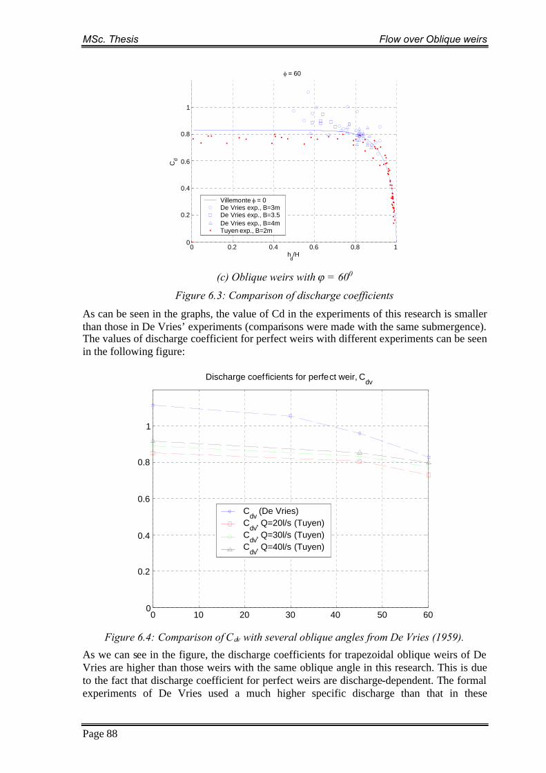
MSc. Thesis Flow over Oblique weirs
Page 88
0 0.2 0.4 0.6 0.8 10
0.2
0.4
0.6
0.8
1
hd/H
Cd
= 60
Villemonte = 0De Vries exp., B=3mDe Vries exp., B=3.5De Vries exp., B=4mTuyen exp., B=2m
(c) Oblique weirs with = 600
Figure 6.3: Comparison of discharge coefficients
As can be seen in the graphs, the value of Cd in the experiments of this research is smallerthan those in De Vries’ experiments (comparisons were made with the same submergence).The values of discharge coefficient for perfect weirs with different experiments can be seenin the following figure:
0 10 20 30 40 50 600
0.2
0.4
0.6
0.8
1
Discharge coefficients for perfect weir, Cdv
Cdv
(De Vries)C
dv, Q=20l/s (Tuyen)
Cdv
, Q=30l/s (Tuyen)C
dv, Q=40l/s (Tuyen)
Figure 6.4: Comparison of Cdv with several oblique angles from De Vries (1959).
As we can see in the figure, the discharge coefficients for trapezoidal oblique weirs of DeVries are higher than those weirs with the same oblique angle in this research. This is dueto the fact that discharge coefficient for perfect weirs are discharge-dependent. The formalexperiments of De Vries used a much higher specific discharge than that in these

MSc. Thesis Flow over Oblique weirs
Page 89
experiments. The high value of Cdv for = 0 (De Vries) may also be due to higher specificdischarge (because the channel width B is much smaller than other cases).
6.2.3. Comparison of results from this research with data from Stelling
As we have discussed earlier, the simple flow model, based on energy conservation,momentum conservation and continuity can be used to predict the flow characteristic.Results from these theoretical analyses have been compared with the measured ones andthere is good agreements between them (see comparisons on losses in chapter 4 andcomparisons on the angle of obliqueness in chapter 5).
The conditions of experiments were used as boundary conditions of the simple flow model.Simulations with inputs are the discharge (upstream condition) and water level downstream(downstream condition) gave outputs as the head loss (h). These calculated values of hwere plotted against the measured one. The differences of experimental and computationalresults can be visualized by the figure below.
0
0.01
0.02
0.03
0.04
0.05
0.06
0.07
0 0.01 0.02 0.03 0.04 0.05 0.06 0.07
Dh Me surem ents
Dh
Sim
ula
tio
ns
Figure 6.4: Comparison of Cdv for plain weir.
The continuous line is the 450 line, whereas the points on graphs are the measured dataversus the computed data. It appears that the model usually under estimated the loss. Thisis explainable because the simple flow model doesn’t take into account the various real-world effects that contribute to the loss in a flow over the weir (where the bottom friction isone of the most important factors).
6.3. Projected discharge coefficientIn chapter 5, the basic assumption for theoretical analysis on flow over oblique weirs hasbeen corroborated. That is, the flow velocity component parallel to the weir crest iseffectively constant everywhere in the area of investigation, i.e. u0L = u1L.= u2L. This can beillustrated by two examples:

MSc. Thesis Flow over Oblique weirs
Page 90
0 0.5 1 1.5 2
0.5
1
1.5
2
0.07
0.08
0.09
0.1
0.11
(a) Q=35l/s
0 0.5 1 1.5 2
0.5
1
1.5
2
0.04
0.05
0.06
0.07
0.08
0.09
0.1
(b) Q=30l/s
Figure 6.6: Velocity component parallel to the weir, =450, Q=30l/s, submerged flow.
In the above mentioned figures, almost no effects of the weir can be observed, but theeffect of the side walls is quite prominent. This velocity component is quite uniform fromupstream of the weir to the downstream area. But across the flume this is not true. (Thereare some small areas with low velocity that might be due to the effect of the oblique weirs).
The idea is that if we can get rid of the side-wall effect, the resulting discharge coefficientwill be much more meaningful. Therefore the following analysis was done in order to findnew discharge coefficient and compare it to the conventional discharge coefficient that hasbeen found in chapter 4.
Data from two different tests were taken to investigate the new Cd: the case of 450 obliquetrapezoidal weirs, submerged flow, Q = 35l/s and Q = 30l/s.

MSc. Thesis Flow over Oblique weirs
Page 91
0 0.5 1 1.5 20
0.02
0.04
0.06
0.08
0.1
0.12
0.14
0.16
0.18
0.2
Lateral distance (m)
Ve
loci
tyco
mpo
nen
tnor
mal
toth
ew
eir(
m/s
)
VELO. VARIATION ALONG THE W.CREST 45 Degrees, Q=35l/s, Submerged flow
(a) Q=35l/s
0 0.2 0.4 0.6 0.8 1 1.2 1.4 1.6 1.8 20
0.02
0.04
0.06
0.08
0.1
0.12
0.14
0.16
0.18
0.2
Lateral distance (m)
Ve
loci
tyc
omp
one
ntn
orm
alto
the
we
ir(m
/s)
(b) Q=30l/s
Figure 6.7: Variation of the perpendicular velocity component along the weir crest,
=450, submerged flow.
The trough in the velocity distribution is due to the low velocity areas in figure 6.6.
Knowing the depth on the weir crest: h1 = 0.0848m and h1 = 0.085m respectively, thedischarge can be found by multiplying h1 with the integration area of the velocity profile.The discharge portion (Qhalf) in exactly 1m in the middle of the flume (from distance +0.5mto distance +1.5m) was also calculated. Cdnew is calculated from this Qhalf and new weirlength (Lhalf).
A difficulty arose during the analysis is that the vector field data from PTV analysisdoesn’t cover the whole length of the weir. The integration length is thus the length of theweir with available data. The flow discharge through this part (Ldata) have to be interpolated
MSc. Thesis Flow over Oblique weirs
Page 92
by assume linear relation between Q and L. This is the weak point of this analysis that needto be improved.
The ratio between new discharge (new discharge coefficient) with previously discharge(previous discharge coefficient) is Rq and RCd respectively.
alconvention
newq Q
QR ;
alconventiond
newdCd C
CR (A.11)
By definition, RQ = RCd.
Result:
- For the case of Q = 35l/s, RQ = RCd = 0.9883- For the case of Q = 30l/s, RQ = RCd = 0.9981
The value of Cd in the middle part of the flume (Cdnew) appeared to be the same with Cdcalculated by the whole flow discharge (Q) and whole channel width (L). This similarmight be the result of some compensation mechanisms between the left part and the rightpart of the flow.
Conclusion:
Due to restrictions in the technique capacity, this analysis has avoided a part of the sidewall effects, but not completely the whole side effects. The resulting discharge coefficientsappeared to be the same as the previously found values. This additional analysisstrengthens the work done by chapter 4. If we skip the regional low velocity areasdownstream of the weir, the new discharge coefficient will slightly increase by a fewpercents depends on the certain case.
It is useful to do this analysis, but further investigations which cover the whole width of thechannel, and investigations with different oblique angle should be conducted. The effect ofthe regional low velocity areas downstream of the weir need to be careful inspected toknow what the real underlying reason is, or it is an artifact due to the experiment conditionof this research only.

MSc. Thesis Flow over Oblique weirs
Page 93
CHAPTER 7. CONCLUSIONS
7.1. Conclusions
Although the weir is a common and standard engineering structure and there is a wideknowledge on perpendicular weirs, few studies have been done on weirs placed obliquelyto the flow direction. With large amount of data obtained with the advanced techniques andinstruments, the experimental and theoretical analysis of this study has provided us withfurther understanding and some specific information regarding the behavior and thecharacteristic of the flow in the neighborhood of the oblique weir. Some main conclusionshad been made as following:
The flow direction in the neighborhood of an oblique weir:The flow always turns its direction when it reaches and passes the weir, towards aperpendicular orientation. Its angle of obliqueness can be well predicted by theoryanalysis (based on energy conservation, momentum conservation, and continuity).Result from PTV analysis shows a good agreement with the theoretically predictedvalues.
Effect of the obliqueness of the weirs:The discharge of an oblique weir is much higher than the discharge of a perpendicularweir with the same channel width because of the higher effective length and a hardlysmaller discharge coefficient. Generally, by increasing the oblique angle () of theweir, the discharge coefficient will slightly decrease and the discharge capacity of theweir will increase.
Discharge reduction coefficient for imperfect weir: Empirical relation of Villemonte (1947) is flexible and works quite well for
all weir configurations have been tested. By applying an appropriate fitparameter, this relation can be used to calculate the discharge coefficient forthe flow in submerged and transition conditions.
Other empirical relations [from Borghei (2003), Seida and Quarashi,Varshney and Mohanty (Kolkman, 1989)...] only fit for certain types of weiror very low submergence (S), thus they are of little use for the weirs in thisresearch.
The simple flow models, together with an experimental determinedreduction coefficient, can work relatively well as a prediction tool, up to ahigh submergence.
Velocity decomposition:The velocity decomposition proves to be an important step in studying the flow over anoblique weir (predicting the angle of obliqueness of the flow, discharge coefficients).The velocity component perpendicular to the weir accounts for the most change in thetotal velocity, whereas the parallel component stays almost unchanged.
Energy dissipation:

MSc. Thesis Flow over Oblique weirs
Page 94
For a perfect weir, the turbulent flow behind weir accounts for the bulk of the energydissipation. Increasing the submergence of the flow, the bottom resistance will play amore and more important role and will dominate the form resistance.
Asymmetry of the flow over an oblique weir:From one side of the flume to the other, there are many differences in flowcharacteristics: the convergence and separation of the flow downstream of the obliqueweir, the vortical movement, the water level and velocity differences, and the flowpattern.
7.2. Feasibility of this study and further research
7.2.1. Accomplishments of this study
The experiment was conducted in the flume for shallow open channel flow. It suits thepurpose of the study well. During the course of the experiments, data was collected andprocessed by both classic instruments and modern techniques. The hydraulics of obliqueweirs has been investigated for many types of weirs, one of which has importantapplication for the understanding of river flow.
Besides the general understanding about physical processes that play a role, this study hasprovided the following:
Extensively simulating and calculating discharge coefficient for flow over physicalmodel of dikes
− Trapezoidal weirs are designed according to dike-design norm− Typical submerged condition in river, and other flow regimes− Investigate discharge capacity for weirs under different angles− Investigate the specific Cd (for the middle part of the flume).
Making use of modern technique to study the flow structure− 3D-distribution of flow velocity− Investigate the oblique angle of the flow over oblique weirs.
Understanding on flow over oblique weirs, especially dike-form weir, can be useful forlong-term programming and policy analysis related to a river delta. It can also be helpful indesigning and amending of constructions in the flood plain and in solving other real-lifeproblems.
7.2.2. Recommendations
Hereafter, some suggestions will be given for further research on the same or related topics.They are laborious and time consuming, but the advantage is accuracy, generality andreliability in the results and conclusions.
Paying more attention to the preliminary period.Experiments first will be carried out on the main straight flume to determine theactual discharge coefficient and different effects of the viscous force, roughnessof the flume, the head loss and energy loss.

MSc. Thesis Flow over Oblique weirs
Page 95
Preliminary experiments on plain weirs (both sharp-crested and broad-crested ifpossible) will be taken to compare the presented discharge coefficients withoblique weirs.
Changing weir configuration in order to understand the influence of other weirparameters (oblique angle, weir form, weir height, crest width, slope).
Experiments will be done with several different oblique angles (including 300)and many more discharge levels to investigate the effect of oblique angle to thedischarge and head loss. The geometry parameter (h0/aw) should also beevaluated by means of changing P as well as H. The upstream vertical wall ofthe weir should be change to a rounded nose or a slope with more streamlinedshape.
Perform experiments with more flow conditions (different specific discharge, Renumber, relative upstream head, and experimental method).
For example this research has investigate the flow over oblique weir for certainrange of relative upstream head (h0/aw = 0.21), other range (0.1, and 1 10)should be investigated as well. The Reynolds number in the tests of this study isin order of 105 (typical value of river flow). Other range of Re should beinvestigated as well.
Applying state-of-art techniques and instruments to study the structure andcharacteristic of the flow (3D-PTV, LDA...)
The three-dimensional structure and behavior of the flow in general and thevelocity distribution and the recirculation zone underneath the flow surface inparticular were only roughly described in this study. They are interesting topicsthat need further research. For all of these research topics a fully 3Dmeasurement technique is of importance. The use of multiple cameras and lasercombines with a three-dimensional particle tracking velocimetry algorithm (3D-PTV) can be a solution.
Performing simulations with better models those are capable of simulating the flowand representing complex phenomena.
** *

MSc. Thesis Flow over Oblique weirs
Page 96
REFERENCES
[1] A.K.A. Maib, 1997, “Fluid mechanics, Hydraulics and Environmental Engineering”,London & Asshford.
[2] B.A.Wols, 2006, “Scheefaangestroomde overlaten”, MSc. Report, Tu Delft.
[3] Borghei et al, 2003, “Discharge coefficient for sharp-crested side weir in subcriticalflow”, Water & Maritime Engineering 156, Issue WM2, pages 185-191.
[4] F.M. Henderson, 1996, “Open channel flow”, Prentice-Hall Inc.[5] G. Bloemberg, 2001, “Stroomlijnen van zomerkaden”, MSc. Report, TU Delft.[6] H. Chanson, 2004, “Environmental Hydraulics of open channel flows”.[7] H. Middelkoop et al, 1999 "Twice a river: Rhine and Meuse in the Netherlands", Rep. 99.003,
RIZA, Arnhem, Netherlands[8] M. Khorchani et al, 2003 "Free surface of flow over side weirs", Science Direct E-journal,
Flow measurement and Instrumentation 15 (2004), page 111-117.[9] M.A.Sarker et al, 2004, “Calculation of free-surface profile over a rectangular broad-crested
weir”, Sciendirect Journal, pages 215-219.[10] M.N.S. Prakash et al, 2004 "Flow over Sharpcrested inclined Inverted V-notch weir", Journal of
Irrigation and Drainage Engineering, volume 130, No.4, August2004.
[11] Munson et al, 2002, “Fundamentals of Fluid Mechanics” 4th edition, John Wiley & Sons,Inc.
[12] P.P.Jansen, 1979, “Principles of River Engineering”.[13] V.T. Chow, 1959, “Open channel flow”, McGraw-Hill International editions, Civil
Engineering series.[14] W.H. Hager, 1994 "Broad crested weir", Journal of Irrigation and Drainage
Engineering, volume 120, No.1, January/February 1994.[15] W.S.J. Uijttewaal et al,
2000,“Effect of shallowness on the development of free-surface mixinglayers”, Journal Physics of fluids volume 12.
[16] W.S.J. Uijttewaal, 2006, “Turbulence in hydraulics CT5312”, lecture notes, TU Delft.

MSc. Thesis Flow over Oblique weirs
Appendices - 1 -
APPENDICES
MSc. Thesis Flow over Oblique weirs
- 2 - Appendices
APPENDIX A: THEORETICAL ISSUES
A.1. Turbulence in the flow and Reynolds stresses(A supplement for§2.2.3)During the experiment process, every test was done on stationary state of the flow. Themeasurement data on velocity (u) is usually collected during a certain time interval, so thatwe can determine a time averaged velocity. This value can be considered as the ensembleaveraged value (u ) due to a rather long averaging period. By the so called Reynoldsdecomposition, instantaneous value of velocity (u) can be considered as the sum of u anda turbulent fluctuation (u’):
'uuu (A.1)The variance of velocity (2) is a measure of the kinetic energy presented in the turbulentfluctuations. And the square root of the variance (||) is the intensity and can be consideredas the mean amplitude of the fluctuation (Ref.2):
22 )( uu . (A.2)Since the flow velocity is usually measured with two components (with an EMF) or three(with an ADV), it is important to define the covariance of each two velocity componentsas:
N
n
nn
Nuu
Nuu
1
)('2
)('121
1lim'' (A.3)
In which N is the number of realizations that constitute the ensemble. Physically, thecovariance represent the transport of momentum (when it is multiplied with the fluiddensity), and can be interpreted as a turbulent shear stress (Ref.2).
Starting from the balance equations for a cubic elementary control volume of fluid in anorthogonal coordinate axes x1, x2, and x3; we come to the continuity equation (theequation on transport of mass) and the three equations on transport of momentum, whichform the Navier-Stokes equation. These four equations form a complete set to describe theflow.For real life flows at moderate and high Reynolds number, no analytical solution for thereequations can be found because of the nonlinear convective transport terms in the Navier-Stokes equations. However for the situation of the experiments on stationary flows in theflume, a proper prediction of the mean flow velocity would be sufficient. Thus we canapply a simplification for the Navier-Stokes equations after decompose the velocity vectors(v
) and the pressure (p) in an ensemble average and a fluctuating component, which yieldsthe so called Reynolds equations (Ref.2):
jjijjiijiij kvpvvvvvt
2'' (A.4)
Or after simplification: jjijijiij kpsvvvt
(A.5)
Where i, j : indicators, taking values of 1, 2 and 3 : gradient operator : the mass density of fluid : the molecular viscosity of fluid, =

MSc. Thesis Flow over Oblique weirs
Appendices - 3 -
: the kinematics viscosity of the fluid; 110-6 m2/s for water.k : source term for momentum, for example the gravity force or Coriolis force.
In the Reynolds equations, the extra terms that stem fromnonlinear advection terms of the Navier-Stokes equationsare denoted as Reynolds stresses:
''jiij vvq (A.6)
The Reynolds stresses represent the effect of thefluctuating velocity components on the mean motion.when i = j, we have q11 , q22, q33 as normal stresseswhen i j, we have six different sij as shear stressesThe stress tensor is illustrated in the figure below.
Figure A1: The stress tensor
A.2. Dimensional analysis, modeling and similitude(A supplement for§3.2.2)
Dimensional analysisPhysical interpretations can be given to dimensionless groups such as the analysis on flowover an oblique weir in chapter 2. This interpretation proves to be very useful for otherparticular application in reality. This type of analysis is called dimensional analysis. Itbased in a consideration of the dimensions of the involved variables.
The non-dimensional groups are also called the dimensionless products, and are frequentlyreferred to as “pi terms” (). Each of the experiment problems can be defined andsimplified by using dimensional analysis with a series of distinct steps. The Froude number(Fr), physically presents the ratio of inertia force and gravitational force, was showed to bethe most common and useful “pi term” for almost all problems in experiments with theopen channel flow. It will be used extensively in this study.
The theory that plays a fundamental role in dimensional analysis is the Buckingham Pitheorem: “If an equation involving k variables is dimensionally homogeneous, it can bereduced to a relationship among (k-r) independent dimensionless products, where r is theminimum number of reference dimensions required to describe the variables” (Munson,2002).
If a set of k variables is considered, the relationship among the pi terms typically has theform of:
rk ,...,, 321 (A.7)Where rk ,...,, 32 is a function of 2 through k-r.
ModelingThe problems of flow over an oblique weir often involve more than two pi terms, thus it isnecessary to develop a model to predict specific characteristics. A (physical scale) model,by definition, is a representation of a physical system that may be used to predict thebehavior of the system in some desired respects. The physical system for which the

MSc. Thesis Flow over Oblique weirs
- 4 - Appendices
predictions are to be made is called the prototype (Munson, 2002). The study on physicalscale model (in this case much smaller than the prototype) will be able to predict thebehavior of the prototype under a certain set of conditions.
Any given problems can be described in terms of the above set of pi terms in equation 3.1.Since the model is governed by the same variables as a particular prototype, a similarrelation ship for the model can be written:
mrkmmm )(321 ,...,, (A.8)
SimilitudeThe similarity between a model and its prototype can be obtained using dimensionlessanalysis. The similarity requirements (or modeling laws) required that the model isdesigned and operated under conditions such that: every pi term (apart from the one pi termthat contain the variable which is to be predicted) of the model is equal to its correspondingpi term of the prototype.
)()(
33
22
...
rkmrk
m
m
(A.9)
Together with the presumption that the form of is the same, it follows by the desiredprediction equation:
m11 (A.10)The above equation indicates that the measured value of 1m during tests with a modelequals to the value of the corresponding1 of the prototype.
A.3. A simple flow model
Review of loss and discharge coefficientDuring the experiment, the head loss was investigated by means of the absolute loss andthe discharge coefficient. When the flow over the weir is critical (perfect weir), thisanalysis proves to be indefectible; and the (specific) discharge can be expressed as anexplicit function of the upstream condition:
2/303
232. HgCq vd (A.12)
In this expression, Cdv is an experimentally determined coefficient to account for thevarious real world effects not included in the simplified analysis to get the actual flow rateas a function of the water head upstream. This analysis is physically meaningful because inthis situation what happen above the weir is completely determined by the upstream flowcondition, it is independent from the downstream flow condition.
Only when the flow is sub-critical (flow in submerged regime), there is no clear relationbetween the flow discharge and the upstream head. For centuries, empirical formulas havebeen evoked to built explicit relations which relate the flow rate to the upstream water head(empirical coefficients like discharge reduction coefficient C*, Ks were introduced toaccount for the reduction in the discharge coefficient and the discharge respectively).
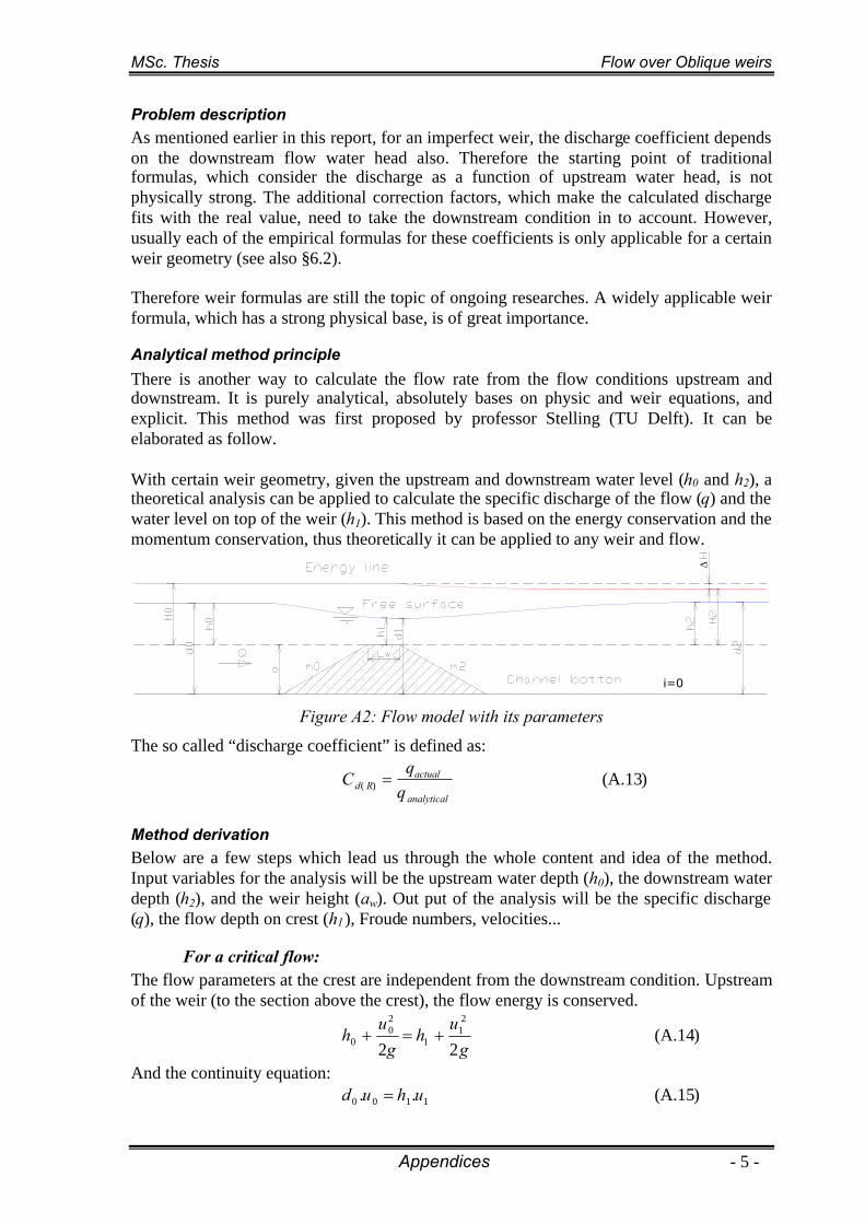
MSc. Thesis Flow over Oblique weirs
Appendices - 5 -
Problem descriptionAs mentioned earlier in this report, for an imperfect weir, the discharge coefficient dependson the downstream flow water head also. Therefore the starting point of traditionalformulas, which consider the discharge as a function of upstream water head, is notphysically strong. The additional correction factors, which make the calculated dischargefits with the real value, need to take the downstream condition in to account. However,usually each of the empirical formulas for these coefficients is only applicable for a certainweir geometry (see also §6.2).
Therefore weir formulas are still the topic of ongoing researches. A widely applicable weirformula, which has a strong physical base, is of great importance.
Analytical method principle
There is another way to calculate the flow rate from the flow conditions upstream anddownstream. It is purely analytical, absolutely bases on physic and weir equations, andexplicit. This method was first proposed by professor Stelling (TU Delft). It can beelaborated as follow.
With certain weir geometry, given the upstream and downstream water level (h0 and h2), atheoretical analysis can be applied to calculate the specific discharge of the flow (q) and thewater level on top of the weir (h1). This method is based on the energy conservation and themomentum conservation, thus theoretically it can be applied to any weir and flow.
i=0
Figure A2: Flow model with its parameters
The so called “discharge coefficient” is defined as:
analytical
actualRd q
qC )( (A.13)
Method derivationBelow are a few steps which lead us through the whole content and idea of the method.Input variables for the analysis will be the upstream water depth (h0), the downstream waterdepth (h2), and the weir height (aw). Out put of the analysis will be the specific discharge(q), the flow depth on crest (h1), Froude numbers, velocities...
For a critical flow:The flow parameters at the crest are independent from the downstream condition. Upstreamof the weir (to the section above the crest), the flow energy is conserved.
gu
hg
uh
22
21
1
20
0 (A.14)
And the continuity equation:1100 .. uhud (A.15)
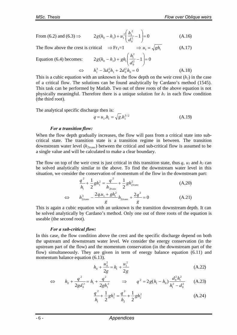
MSc. Thesis Flow over Oblique weirs
- 6 - Appendices
From (6.2) and (6.3) 01)(2 20
212
110
dh
uhhg (A.16)
The flow above the crest is critical Fr1=1 11 ghu (A.17)
Equation (6.4) becomes: 01)(2 20
21
110
dh
ghhhg
023 0201
20
31 hdhdh (A.18)
This is a cubic equation with an unknown is the flow depth on the weir crest (h1) in the caseof a critical flow. The solutions can be found analytically by Cardano’s method (1545).This task can be performed by Matlab. Two out of three roots of the above equation is notphysically meaningful. Therefore there is a unique solution for h1 in each flow condition(the third root).
The analytical specific discharge then is:2/3
111 .. hghuq (A.19)
For a transition flow:When the flow depth gradually increases, the flow will pass from a critical state into sub-critical state. The transition state is a transition regime in between. The transitiondownstream water level (h2trans) between the critical and sub-critical flow is assumed to bea single value and will be calculated to make a clear boundary.
The flow on top of the weir crest is just critical in this transition state, thus q, u1 and h1 canbe solved analytically similar to the above. To find the downstream water level in thissituation, we consider the conservation of momentum of the flow in the downstream part:
22
2
221
1
2
21
21
transtrans
ghh
qghhq (A,20)
02.2 2
2
2113
2
gqh
gghuq
h transtrans (A.21)
This is again a cubic equation with an unknown is the transition downstream depth. It canbe solved analytically by Cardano’s method. Only one out of three roots of the equation isuseable (the second root).
For a sub-critical flow:In this case, the flow condition above the crest and the specific discharge depend on boththe upstream and downstream water level. We consider the energy conservation (in theupstream part of the flow) and the momentum conservation (in the downstream part of theflow) simultaneously. They are given in term of energy balance equation (6.11) andmomentum balance equation (6.13).
gu
hg
uh
22
21
1
20
0 (A.22)
2
1
2
120
2
0 22 ghqh
gdqh
20
21
21
20
012 )(2
dhhd
hhgq
(A.23)
22
2
221
1
2
21
21 gh
hqgh
hq (A.24)

MSc. Thesis Flow over Oblique weirs
Appendices - 7 -
21
22
21
2
2111
ddgdh
q
12
2121
22
2
21
hddh
ddgq
(A.25)
Together from (6.12) and (6.14), an equation for h1 was found as follow: 0.4 2
20
21
21
22121
2001 ddhddhdhdhh (A.26)
From this equation, h1 can be found by several methods. We may apply the bi-sectionmethod here or using Matlab to find roots for the 3rd order polynomial of h1. As h1 wasfound, other parameters (q, u1, u0, u2, Fr0, Fr1, Fr2...) can be easily calculated from thisvalue.
We will refer to this method as “complex” method from now on.
Method judgementA comparison was made to evaluate the performance of the analytical method and thereliability of the measurement data. The above flow model was tested with the same weirgeometry and flow parameters. The measured values of q from experiments were taken asqactual.
In the figure below Cd(R) was plotted against the submergence S. Two cases can bedistinguished: with and without bottom friction. The loss due to bottom friction alone(without any weirs) was estimated from measurements and taken into account whencalculate q and h1 in the present of a weir.
0 0.2 0.4 0.6 0.8 10.4
0.5
0.6
0.7
0.8
0.9
1
Submergence (-)
Cd(
R)=
q exp/q
ana
(-)
Cd(R)
(Bottom friction = 0)
Cd(R)
(Bottom friction # 0)
Figure A3: Cd(R) with and without bottom friction
Without taking into account all the phenomena and parameters that play a role in the flowover a weir, the flow model as above usually over estimate the flow discharge, i.e. Cd(R)1.Typical value of Cd(R) is 0.87 according to these calculations. As we can see from thefigure, the consideration of the loss caused by bottom friction makes predictions made bythe model come closer to reality. Especially in the region of high submergence, this changecauses a smaller range of deviation for )(RdC from its mean value.

MSc. Thesis Flow over Oblique weirs
- 8 - Appendices
This coefficient shows quite some scatters: the higher the specific discharge q, the higherthe Cd(R). This can be illustrated by the following figure.
0 0.2 0.4 0.6 0.8 10.4
0.5
0.6
0.7
0.8
0.9
1
Submergence (-)
Cd
(R)=
q exp/q
ana
(-)
Cd(R)
(q = 0.01 m2/s)
Cd(R)
(q = 0.015 m2/s)
Cd(R)
(q = 0.02 m2/s)
Figure A4: Cd(R) for different specific discharges
Most of the cases (when S 0.9) the relation between analytical q and measured q isalmost a constant. By determining this constant from experiments, we can use the abovemodel to predict the specific discharge for the prototype in a comparable condition.
Cd(R) shows bigger deviation from its mean value at high submergence. This can beexplained by the increasing effect of the bottom friction (it becomes more and moreimportant) as the flow changes to sub-critical condition. Especial at very highsubmergence, there is hardly any effects of the weir (the flow surface is nearly horizontal),and the loss caused by bottom friction is dominated.
Introduction of new weir formulasLeft alone the gap between (rough) analytical prediction and reality, in the following partwe will investigate the empirical formula introduced by professor G.S.Stelling (TU Delft)and the possibilities of other empirical relations.
For the shake of simplicity, Stelling introduced an empirical formula for calculating thewater depth on top of a weir crest:
)( 1020
2211 crit
trans
transcrit hh
hhhh
hh
(A.27)
in which: h1crit : the water depth on top of the weir crest in the critical flowh2trans : the transition downstream water depth (as mentioned earlier)
In general, the empirical formula of Stelling does a good job by giving a value of h1 (h1emp)close to the value which is obtained by the complex theoretical analysis (h1comp). Thedifference is usually smaller than 2%. The specific discharge calculated from this waterdepth (qemp) has a pretty good agreement with the specific discharge by calculated bycomplex method (qcomp) in the region of low submergence (S<0.8). However, qemp shows
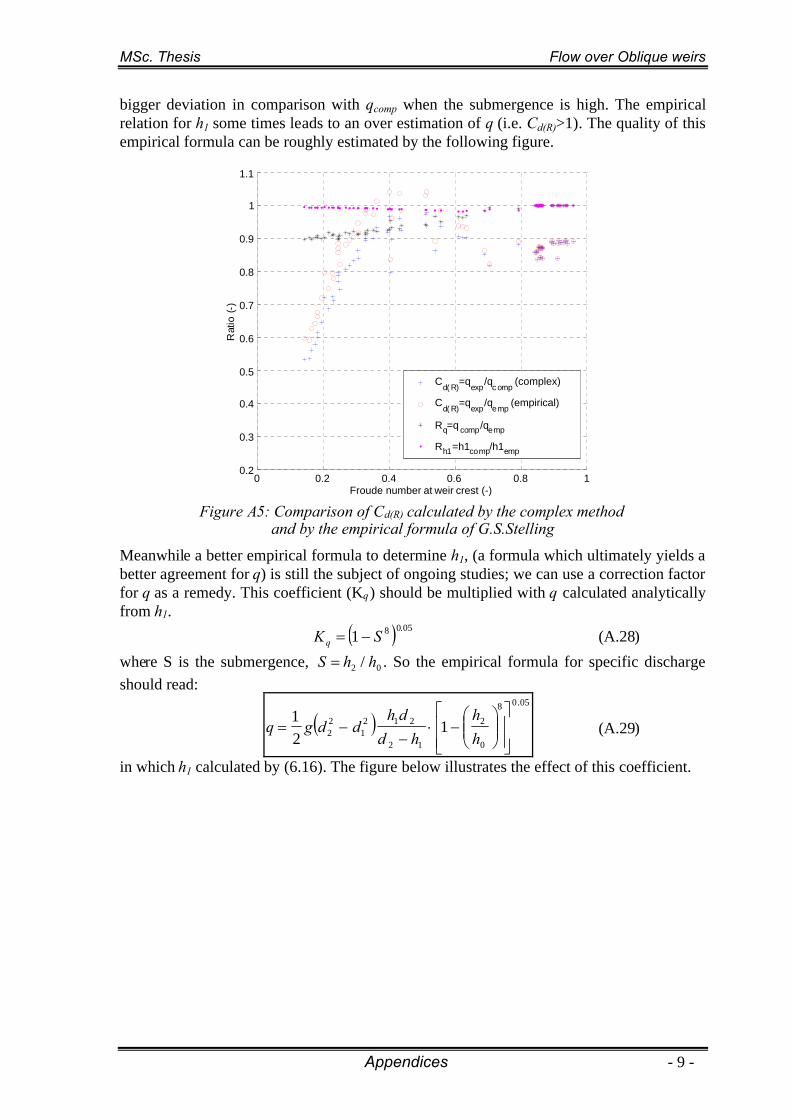
MSc. Thesis Flow over Oblique weirs
Appendices - 9 -
bigger deviation in comparison with qcomp when the submergence is high. The empiricalrelation for h1 some times leads to an over estimation of q (i.e. Cd(R)>1). The quality of thisempirical formula can be roughly estimated by the following figure.
0 0.2 0.4 0.6 0.8 10.2
0.3
0.4
0.5
0.6
0.7
0.8
0.9
1
1.1
Froude number at weir crest (-)
Rat
io(-
)
Cd( R)
=qexp
/qc omp
(complex)
Cd( R)
=qexp
/qemp
(empirical)
Rq=q comp/qemp
Rh1=h1comp/h1emp
Figure A5: Comparison of Cd(R) calculated by the complex methodand by the empirical formula of G.S.Stelling
Meanwhile a better empirical formula to determine h1, (a formula which ultimately yields abetter agreement for q) is still the subject of ongoing studies; we can use a correction factorfor q as a remedy. This coefficient (Kq) should be multiplied with q calculated analyticallyfrom h1.
05.081 SKq (A.28)
where S is the submergence, 02 / hhS . So the empirical formula for specific dischargeshould read:
05.08
0
2
12
2121
22 1
21
hh
hddh
ddgq (A.29)
in which h1 calculated by (6.16). The figure below illustrates the effect of this coefficient.

MSc. Thesis Flow over Oblique weirs
- 10 - Appendices
0.6 0.65 0.7 0.75 0.8 0.85 0.9 0.95 10.8
0.85
0.9
0.95
1
1.05
Submergence (-)
Rat
io(-)
Rq=qcomp/qemp (Stelling)
Rq=Kq*(qcomp/qemp) (Tuyen)
Rh1=h1comp/h1emp
Figure A6: Differences between flow parameters calculated by different methods
The correction factor Kq reduces the difference between qcomp and qemp from more than 10%to around 2%. The two empirical formulas (A.27) and (A.29) now can be used to calculateh1 and q with the same order of accuracy about 2% (in comparison with the complexmethod).
Conclusions:This analytical method of calculating the discharge reduction coefficient is completelyexplicit, that is the strong point. It is based on physic and able to make prediction to thespecific discharge, although an experimental determined reduction factor need to beincluded.
The empirical of Stelling appears to be complicated, but it works quite well for theprediction of water depth on top of the weir crest. Only for the specific discharge thatderives from this value of water depth there is a 10% deviation from the expected value. Acorrection parameter needs to be added. This formula looks more complicated thanavailable empirical formulas, but hopefully it hasn’t got the short-coming of them, i.e. itcan work equally well for all types of weir.

MSc. Thesis Flow over Oblique weirs
Appendices - 11 -
APPENDIX B: LOSS MEASUREMENTS AND ANALYSIS
Loss measurements were performed on different weir forms and oblique angles. Eachconfiguration of the weir required a series of tests. The trapezoidal weir form plays themost important role and has been studied extensively in this research. Hereafter, mostimportant data and results for trapezoidal weir will be summarized in a separated table.
B.1. Trapezoidal weir, = 00
Q (l/s) = 20 ÷ 40 H0 (m) = -phi (0) = 0 B (m) = 2
Cdv = 0.889 Weir height a (cm) = 10.4Fit parameter p = 18 g (m/s2) = 9.81
Table B1: Loss measurements for trapezoidal weir, = 00.
Qh0 (at x = -100cm) h1 (at x = 0cm) Fr1
h2 (atx=+400cm) S Cd C* H0/aExp.
No.(l/s) h0 + a H0 (cm) h1 + a h1
(cm)H1
(cm)- h2 + a H2
(cm)(H2/H0) Measured -
1 40 15.87 5.47 13.94 3.54 3.56 0.96 14.19 3.79 0.69 0.92 1.03 0.532 40 15.95 5.55 14.23 3.83 3.84 0.85 14.95 4.55 0.82 0.90 1.01 0.533 40 16.37 5.97 15.12 4.72 4.73 0.62 15.92 5.52 0.92 0.80 0.90 0.574 40 15.99 5.59 14.42 4.02 4.03 0.79 15.22 4.82 0.86 0.89 1.00 0.545 40 16.61 6.21 15.48 5.08 5.09 0.56 16.27 5.87 0.95 0.76 0.85 0.606 40 17.24 6.84 16.43 6.03 6.04 0.43 17.02 6.62 0.97 0.66 0.74 0.667 40 16.78 6.38 15.78 5.38 5.39 0.51 16.51 6.11 0.96 0.73 0.82 0.618 40 17.56 7.16 16.77 6.37 6.38 0.40 17.35 6.95 0.97 0.61 0.69 0.699 40 18.29 7.89 17.62 7.22 7.22 0.33 18.13 7.73 0.98 0.53 0.60 0.76
10 40 19.78 9.38 19.18 8.78 8.78 0.25 19.65 9.25 0.99 0.41 0.46 0.9011 40 15.86 5.46 13.99 3.59 3.61 0.94 9.70 -0.70 -0.13 0.92 1.03 0.5312 40 15.87 5.47 14.11 3.71 3.72 0.89 10.57 0.17 0.03 0.92 1.03 0.5313 40 16.33 5.93 15.18 4.78 4.79 0.61 15.87 5.47 0.92 0.81 0.91 0.5714 40 15.86 5.46 14.05 3.65 3.67 0.92 12.66 2.26 0.41 0.92 1.03 0.5315 40 15.87 5.47 14.00 3.60 3.62 0.93 13.89 3.49 0.64 0.92 1.03 0.5316 35 17.94 7.54 17.33 6.93 6.93 0.31 17.78 7.38 0.98 0.50 0.56 0.7317 35 16.88 6.48 16.18 5.78 5.78 0.40 16.69 6.29 0.97 0.62 0.70 0.6218 35 15.44 5.04 13.68 3.28 3.29 0.94 13.42 3.02 0.60 0.91 1.02 0.4819 35 15.43 5.03 13.73 3.33 3.34 0.92 13.14 2.74 0.54 0.91 1.02 0.4820 35 15.81 5.41 14.66 4.26 4.27 0.64 15.35 4.95 0.91 0.82 0.92 0.5221 35 16.23 5.83 15.33 4.93 4.94 0.51 15.96 5.56 0.95 0.73 0.82 0.5622 35 16.85 6.45 16.13 5.73 5.73 0.41 16.62 6.22 0.96 0.63 0.70 0.6223 35 17.27 6.87 16.58 6.18 6.18 0.36 17.10 6.70 0.98 0.57 0.64 0.6624 35 17.62 7.22 17.02 6.62 6.62 0.33 17.46 7.06 0.98 0.53 0.60 0.6925 35 17.95 7.55 17.35 6.95 6.95 0.30 17.80 7.40 0.98 0.49 0.56 0.7326 35 18.97 8.57 18.43 8.03 8.03 0.25 18.85 8.45 0.99 0.41 0.46 0.8227 35 15.43 5.03 13.80 3.40 3.41 0.89 13.31 2.91 0.58 0.91 1.02 0.4828 35 15.44 5.04 13.75 3.35 3.36 0.91 10.66 0.26 0.05 0.91 1.02 0.4829 35 15.44 5.04 13.78 3.38 3.39 0.90 11.57 1.17 0.23 0.91 1.02 0.4830 35 15.43 5.03 13.71 3.31 3.32 0.93 12.02 1.62 0.32 0.91 1.02 0.4831 30 16.71 6.31 16.10 5.70 5.70 0.35 16.54 6.14 0.97 0.56 0.62 0.6132 30 16.05 5.65 15.33 4.93 4.93 0.44 15.82 5.42 0.96 0.66 0.74 0.5433 30 15.24 4.84 14.04 3.64 3.65 0.69 14.64 4.24 0.88 0.83 0.93 0.4734 30 15.01 4.61 13.53 3.13 3.14 0.86 13.89 3.49 0.76 0.89 1.00 0.4435 30 15.00 4.60 13.53 3.13 3.14 0.86 12.49 2.09 0.45 0.89 1.00 0.44

MSc. Thesis Flow over Oblique weirs
- 12 - Appendices
Q h0 (at x = -100cm) h1 (at x = 0cm) Fr1
h2 (atx=+400cm) S Cd C* H0/aExp.
No.(l/s) h0 + a H0 (cm) h1 + a
h1(cm)
H1(cm) - h2 + a
H2(cm) (H2/H0) Measured -
36 30 14.99 4.59 13.55 3.15 3.16 0.86 11.76 1.36 0.30 0.89 1.01 0.4437 30 15.00 4.60 13.54 3.14 3.15 0.86 10.57 0.17 0.04 0.89 1.00 0.4438 30 18.17 7.77 17.65 7.25 7.25 0.25 18.05 7.65 0.98 0.41 0.46 0.7539 30 19.31 8.91 18.83 8.43 8.43 0.20 19.19 8.79 0.99 0.33 0.37 0.8640 30 18.07 7.67 17.54 7.14 7.14 0.25 17.93 7.53 0.98 0.41 0.47 0.7441 30 17.59 7.19 17.03 6.63 6.63 0.28 17.45 7.05 0.98 0.46 0.51 0.6942 30 15.01 4.61 13.54 3.14 3.15 0.86 10.80 0.40 0.09 0.89 1.00 0.4443 30 15.00 4.60 13.55 3.15 3.16 0.86 11.54 1.14 0.25 0.89 1.00 0.4444 25 18.14 7.74 17.65 7.25 7.25 0.20 18.04 7.64 0.99 0.34 0.38 0.7445 25 18.69 8.29 18.22 7.82 7.82 0.18 18.57 8.17 0.99 0.31 0.35 0.8046 25 19.30 8.90 18.80 8.40 8.40 0.16 19.19 8.79 0.99 0.28 0.31 0.8647 25 18.87 8.47 18.39 7.99 7.99 0.18 18.75 8.35 0.99 0.30 0.33 0.8148 25 17.65 7.25 17.17 6.77 6.77 0.23 17.53 7.13 0.98 0.38 0.42 0.7049 25 16.64 6.24 16.12 5.72 5.72 0.29 16.50 6.10 0.98 0.47 0.53 0.6050 25 14.52 4.12 13.21 2.81 2.82 0.85 11.51 1.11 0.27 0.88 0.99 0.4051 25 16.23 5.83 15.63 5.23 5.23 0.33 16.09 5.69 0.98 0.52 0.59 0.5652 25 16.93 6.53 16.44 6.04 6.04 0.27 16.80 6.40 0.98 0.44 0.49 0.6353 25 17.55 7.15 17.05 6.65 6.65 0.23 17.42 7.02 0.98 0.38 0.43 0.6954 25 14.51 4.11 13.20 2.80 2.81 0.85 12.50 2.10 0.51 0.88 0.99 0.4055 25 14.53 4.13 13.21 2.81 2.82 0.85 12.94 2.54 0.62 0.87 0.98 0.4056 25 14.53 4.13 13.22 2.82 2.83 0.84 11.25 0.85 0.21 0.87 0.98 0.4057 25 15.00 4.60 14.20 3.80 3.81 0.54 14.63 4.23 0.92 0.74 0.84 0.4458 20 18.86 8.46 18.34 7.94 7.94 0.14 18.77 8.37 0.99 0.24 0.27 0.8159 20 14.01 3.61 12.80 2.39 2.40 0.86 9.97 -0.43 -0.12 0.86 0.96 0.3560 20 14.03 3.63 12.82 2.41 2.42 0.85 12.70 2.30 0.63 0.85 0.95 0.3561 20 14.02 3.62 12.71 2.30 2.31 0.91 11.93 1.53 0.42 0.85 0.96 0.3562 20 14.14 3.74 13.14 2.73 2.74 0.71 13.53 3.13 0.84 0.81 0.91 0.3663 20 14.92 4.52 14.36 3.96 3.96 0.40 14.66 4.26 0.94 0.61 0.69 0.4364 20 16.06 5.66 15.69 5.29 5.29 0.26 16.00 5.60 0.99 0.44 0.49 0.5465 20 16.83 6.43 16.41 6.01 6.01 0.22 16.71 6.31 0.98 0.36 0.40 0.6266 20 17.56 7.16 17.14 6.74 6.74 0.18 17.45 7.05 0.98 0.31 0.34 0.6967 20 18.29 7.89 17.85 7.45 7.45 0.16 18.18 7.78 0.99 0.26 0.30 0.7668 20 14.02 3.62 12.79 2.38 2.39 0.86 11.22 0.82 0.23 0.85 0.96 0.3569 20 14.01 3.61 12.80 2.39 2.40 0.86 10.57 0.17 0.05 0.86 0.96 0.35
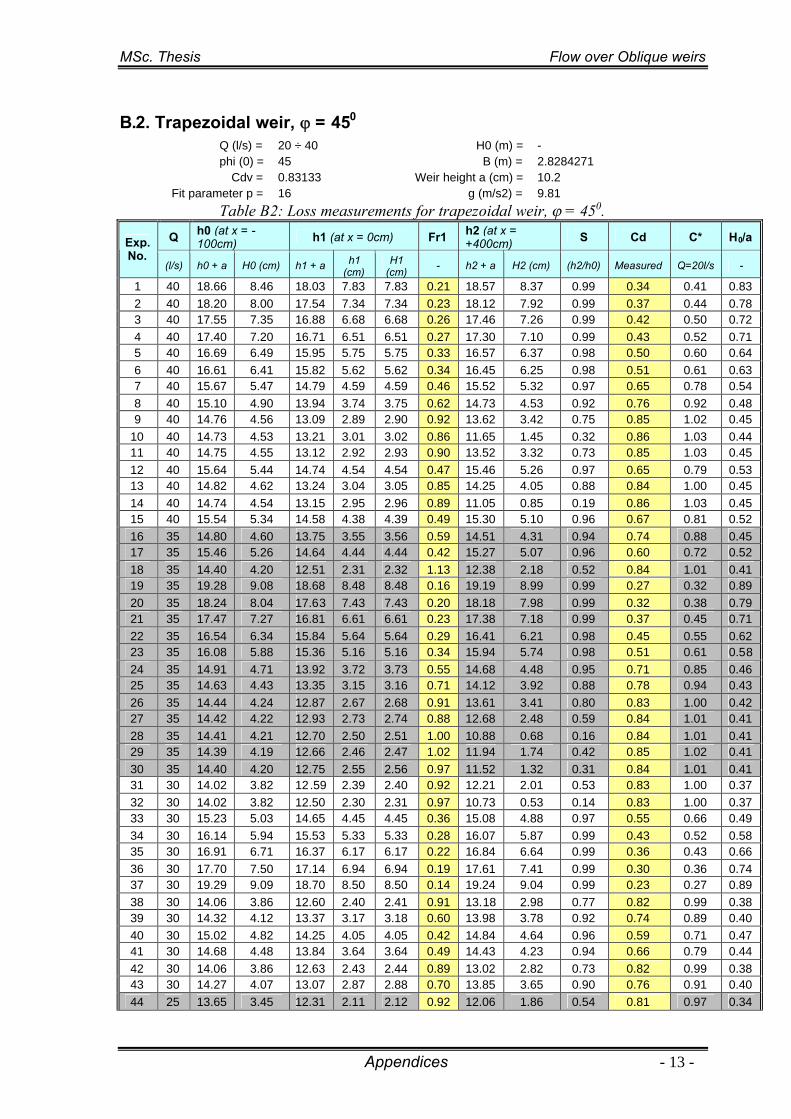
MSc. Thesis Flow over Oblique weirs
Appendices - 13 -
B.2. Trapezoidal weir, = 450
Q (l/s) = 20 ÷ 40 H0 (m) = -phi (0) = 45 B (m) = 2.8284271
Cdv = 0.83133 Weir height a (cm) = 10.2Fit parameter p = 16 g (m/s2) = 9.81
Table B2: Loss measurements for trapezoidal weir, = 450.
Q h0 (at x = -100cm) h1 (at x = 0cm) Fr1 h2 (at x =
+400cm) S Cd C* H0/aExp.No.
(l/s) h0 + a H0 (cm) h1 + a h1(cm)
H1(cm)
- h2 + a H2 (cm) (h2/h0) Measured Q=20l/s -
1 40 18.66 8.46 18.03 7.83 7.83 0.21 18.57 8.37 0.99 0.34 0.41 0.832 40 18.20 8.00 17.54 7.34 7.34 0.23 18.12 7.92 0.99 0.37 0.44 0.783 40 17.55 7.35 16.88 6.68 6.68 0.26 17.46 7.26 0.99 0.42 0.50 0.724 40 17.40 7.20 16.71 6.51 6.51 0.27 17.30 7.10 0.99 0.43 0.52 0.715 40 16.69 6.49 15.95 5.75 5.75 0.33 16.57 6.37 0.98 0.50 0.60 0.646 40 16.61 6.41 15.82 5.62 5.62 0.34 16.45 6.25 0.98 0.51 0.61 0.637 40 15.67 5.47 14.79 4.59 4.59 0.46 15.52 5.32 0.97 0.65 0.78 0.548 40 15.10 4.90 13.94 3.74 3.75 0.62 14.73 4.53 0.92 0.76 0.92 0.489 40 14.76 4.56 13.09 2.89 2.90 0.92 13.62 3.42 0.75 0.85 1.02 0.45
10 40 14.73 4.53 13.21 3.01 3.02 0.86 11.65 1.45 0.32 0.86 1.03 0.4411 40 14.75 4.55 13.12 2.92 2.93 0.90 13.52 3.32 0.73 0.85 1.03 0.4512 40 15.64 5.44 14.74 4.54 4.54 0.47 15.46 5.26 0.97 0.65 0.79 0.5313 40 14.82 4.62 13.24 3.04 3.05 0.85 14.25 4.05 0.88 0.84 1.00 0.4514 40 14.74 4.54 13.15 2.95 2.96 0.89 11.05 0.85 0.19 0.86 1.03 0.4515 40 15.54 5.34 14.58 4.38 4.39 0.49 15.30 5.10 0.96 0.67 0.81 0.5216 35 14.80 4.60 13.75 3.55 3.56 0.59 14.51 4.31 0.94 0.74 0.88 0.4517 35 15.46 5.26 14.64 4.44 4.44 0.42 15.27 5.07 0.96 0.60 0.72 0.5218 35 14.40 4.20 12.51 2.31 2.32 1.13 12.38 2.18 0.52 0.84 1.01 0.4119 35 19.28 9.08 18.68 8.48 8.48 0.16 19.19 8.99 0.99 0.27 0.32 0.8920 35 18.24 8.04 17.63 7.43 7.43 0.20 18.18 7.98 0.99 0.32 0.38 0.7921 35 17.47 7.27 16.81 6.61 6.61 0.23 17.38 7.18 0.99 0.37 0.45 0.7122 35 16.54 6.34 15.84 5.64 5.64 0.29 16.41 6.21 0.98 0.45 0.55 0.6223 35 16.08 5.88 15.36 5.16 5.16 0.34 15.94 5.74 0.98 0.51 0.61 0.5824 35 14.91 4.71 13.92 3.72 3.73 0.55 14.68 4.48 0.95 0.71 0.85 0.4625 35 14.63 4.43 13.35 3.15 3.16 0.71 14.12 3.92 0.88 0.78 0.94 0.4326 35 14.44 4.24 12.87 2.67 2.68 0.91 13.61 3.41 0.80 0.83 1.00 0.4227 35 14.42 4.22 12.93 2.73 2.74 0.88 12.68 2.48 0.59 0.84 1.01 0.4128 35 14.41 4.21 12.70 2.50 2.51 1.00 10.88 0.68 0.16 0.84 1.01 0.4129 35 14.39 4.19 12.66 2.46 2.47 1.02 11.94 1.74 0.42 0.85 1.02 0.4130 35 14.40 4.20 12.75 2.55 2.56 0.97 11.52 1.32 0.31 0.84 1.01 0.4131 30 14.02 3.82 12.59 2.39 2.40 0.92 12.21 2.01 0.53 0.83 1.00 0.3732 30 14.02 3.82 12.50 2.30 2.31 0.97 10.73 0.53 0.14 0.83 1.00 0.3733 30 15.23 5.03 14.65 4.45 4.45 0.36 15.08 4.88 0.97 0.55 0.66 0.4934 30 16.14 5.94 15.53 5.33 5.33 0.28 16.07 5.87 0.99 0.43 0.52 0.5835 30 16.91 6.71 16.37 6.17 6.17 0.22 16.84 6.64 0.99 0.36 0.43 0.6636 30 17.70 7.50 17.14 6.94 6.94 0.19 17.61 7.41 0.99 0.30 0.36 0.7437 30 19.29 9.09 18.70 8.50 8.50 0.14 19.24 9.04 0.99 0.23 0.27 0.8938 30 14.06 3.86 12.60 2.40 2.41 0.91 13.18 2.98 0.77 0.82 0.99 0.3839 30 14.32 4.12 13.37 3.17 3.18 0.60 13.98 3.78 0.92 0.74 0.89 0.4040 30 15.02 4.82 14.25 4.05 4.05 0.42 14.84 4.64 0.96 0.59 0.71 0.4741 30 14.68 4.48 13.84 3.64 3.64 0.49 14.43 4.23 0.94 0.66 0.79 0.4442 30 14.06 3.86 12.63 2.43 2.44 0.89 13.02 2.82 0.73 0.82 0.99 0.3843 30 14.27 4.07 13.07 2.87 2.88 0.70 13.85 3.65 0.90 0.76 0.91 0.4044 25 13.65 3.45 12.31 2.11 2.12 0.92 12.06 1.86 0.54 0.81 0.97 0.34
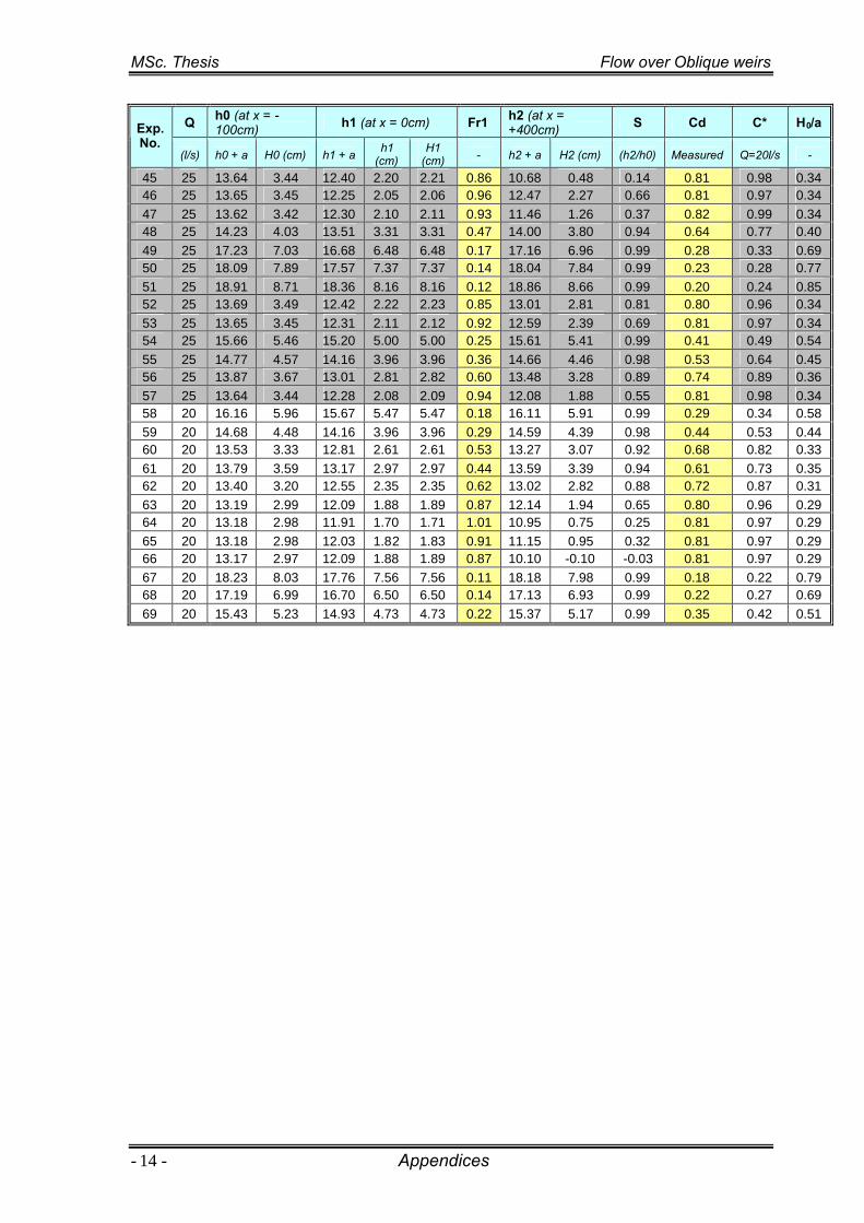
MSc. Thesis Flow over Oblique weirs
- 14 - Appendices
Q h0 (at x = -100cm) h1 (at x = 0cm) Fr1 h2 (at x =
+400cm) S Cd C* H0/aExp.No.
(l/s) h0 + a H0 (cm) h1 + ah1
(cm)H1
(cm) - h2 + a H2 (cm) (h2/h0) Measured Q=20l/s -
45 25 13.64 3.44 12.40 2.20 2.21 0.86 10.68 0.48 0.14 0.81 0.98 0.3446 25 13.65 3.45 12.25 2.05 2.06 0.96 12.47 2.27 0.66 0.81 0.97 0.3447 25 13.62 3.42 12.30 2.10 2.11 0.93 11.46 1.26 0.37 0.82 0.99 0.3448 25 14.23 4.03 13.51 3.31 3.31 0.47 14.00 3.80 0.94 0.64 0.77 0.4049 25 17.23 7.03 16.68 6.48 6.48 0.17 17.16 6.96 0.99 0.28 0.33 0.6950 25 18.09 7.89 17.57 7.37 7.37 0.14 18.04 7.84 0.99 0.23 0.28 0.7751 25 18.91 8.71 18.36 8.16 8.16 0.12 18.86 8.66 0.99 0.20 0.24 0.8552 25 13.69 3.49 12.42 2.22 2.23 0.85 13.01 2.81 0.81 0.80 0.96 0.3453 25 13.65 3.45 12.31 2.11 2.12 0.92 12.59 2.39 0.69 0.81 0.97 0.3454 25 15.66 5.46 15.20 5.00 5.00 0.25 15.61 5.41 0.99 0.41 0.49 0.5455 25 14.77 4.57 14.16 3.96 3.96 0.36 14.66 4.46 0.98 0.53 0.64 0.4556 25 13.87 3.67 13.01 2.81 2.82 0.60 13.48 3.28 0.89 0.74 0.89 0.3657 25 13.64 3.44 12.28 2.08 2.09 0.94 12.08 1.88 0.55 0.81 0.98 0.3458 20 16.16 5.96 15.67 5.47 5.47 0.18 16.11 5.91 0.99 0.29 0.34 0.5859 20 14.68 4.48 14.16 3.96 3.96 0.29 14.59 4.39 0.98 0.44 0.53 0.4460 20 13.53 3.33 12.81 2.61 2.61 0.53 13.27 3.07 0.92 0.68 0.82 0.3361 20 13.79 3.59 13.17 2.97 2.97 0.44 13.59 3.39 0.94 0.61 0.73 0.3562 20 13.40 3.20 12.55 2.35 2.35 0.62 13.02 2.82 0.88 0.72 0.87 0.3163 20 13.19 2.99 12.09 1.88 1.89 0.87 12.14 1.94 0.65 0.80 0.96 0.2964 20 13.18 2.98 11.91 1.70 1.71 1.01 10.95 0.75 0.25 0.81 0.97 0.2965 20 13.18 2.98 12.03 1.82 1.83 0.91 11.15 0.95 0.32 0.81 0.97 0.2966 20 13.17 2.97 12.09 1.88 1.89 0.87 10.10 -0.10 -0.03 0.81 0.97 0.2967 20 18.23 8.03 17.76 7.56 7.56 0.11 18.18 7.98 0.99 0.18 0.22 0.7968 20 17.19 6.99 16.70 6.50 6.50 0.14 17.13 6.93 0.99 0.22 0.27 0.6969 20 15.43 5.23 14.93 4.73 4.73 0.22 15.37 5.17 0.99 0.35 0.42 0.51
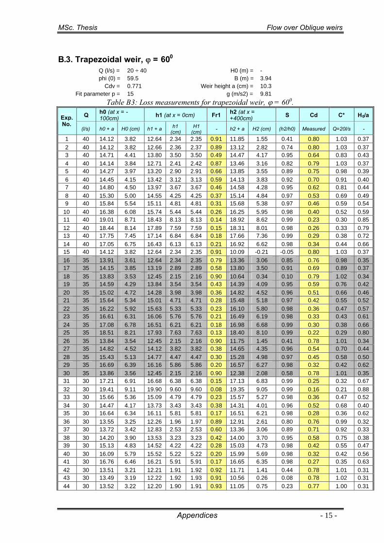
MSc. Thesis Flow over Oblique weirs
Appendices - 15 -
B.3. Trapezoidal weir, = 600
Q (l/s) = 20 ÷ 40 H0 (m) = -phi (0) = 59.5 B (m) = 3.94
Cdv = 0.771 Weir height a (cm) = 10.3Fit parameter p = 15 g (m/s2) = 9.81
Table B3: Loss measurements for trapezoidal weir, = 600.
Q h0 (at x = -100cm) h1 (at x = 0cm) Fr1 h2 (at x =
+400cm) S Cd C* H0/aExp.No.
(l/s) h0 + a H0 (cm) h1 + a h1(cm)
H1(cm)
- h2 + a H2 (cm) (h2/h0) Measured Q=20l/s -
1 40 14.12 3.82 12.64 2.34 2.35 0.91 11.85 1.55 0.41 0.80 1.03 0.372 40 14.12 3.82 12.66 2.36 2.37 0.89 13.12 2.82 0.74 0.80 1.03 0.373 40 14.71 4.41 13.80 3.50 3.50 0.49 14.47 4.17 0.95 0.64 0.83 0.434 40 14.14 3.84 12.71 2.41 2.42 0.87 13.46 3.16 0.82 0.79 1.03 0.375 40 14.27 3.97 13.20 2.90 2.91 0.66 13.85 3.55 0.89 0.75 0.98 0.396 40 14.45 4.15 13.42 3.12 3.13 0.59 14.13 3.83 0.92 0.70 0.91 0.407 40 14.80 4.50 13.97 3.67 3.67 0.46 14.58 4.28 0.95 0.62 0.81 0.448 40 15.30 5.00 14.55 4.25 4.25 0.37 15.14 4.84 0.97 0.53 0.69 0.499 40 15.84 5.54 15.11 4.81 4.81 0.31 15.68 5.38 0.97 0.46 0.59 0.54
10 40 16.38 6.08 15.74 5.44 5.44 0.26 16.25 5.95 0.98 0.40 0.52 0.5911 40 19.01 8.71 18.43 8.13 8.13 0.14 18.92 8.62 0.99 0.23 0.30 0.8512 40 18.44 8.14 17.89 7.59 7.59 0.15 18.31 8.01 0.98 0.26 0.33 0.7913 40 17.75 7.45 17.14 6.84 6.84 0.18 17.66 7.36 0.99 0.29 0.38 0.7214 40 17.05 6.75 16.43 6.13 6.13 0.21 16.92 6.62 0.98 0.34 0.44 0.6615 40 14.12 3.82 12.64 2.34 2.35 0.91 10.09 -0.21 -0.05 0.80 1.03 0.3716 35 13.91 3.61 12.64 2.34 2.35 0.79 13.36 3.06 0.85 0.76 0.98 0.3517 35 14.15 3.85 13.19 2.89 2.89 0.58 13.80 3.50 0.91 0.69 0.89 0.3718 35 13.83 3.53 12.45 2.15 2.16 0.90 10.64 0.34 0.10 0.79 1.02 0.3419 35 14.59 4.29 13.84 3.54 3.54 0.43 14.39 4.09 0.95 0.59 0.76 0.4220 35 15.02 4.72 14.28 3.98 3.98 0.36 14.82 4.52 0.96 0.51 0.66 0.4621 35 15.64 5.34 15.01 4.71 4.71 0.28 15.48 5.18 0.97 0.42 0.55 0.5222 35 16.22 5.92 15.63 5.33 5.33 0.23 16.10 5.80 0.98 0.36 0.47 0.5723 35 16.61 6.31 16.06 5.76 5.76 0.21 16.49 6.19 0.98 0.33 0.43 0.6124 35 17.08 6.78 16.51 6.21 6.21 0.18 16.98 6.68 0.99 0.30 0.38 0.6625 35 18.51 8.21 17.93 7.63 7.63 0.13 18.40 8.10 0.99 0.22 0.29 0.8026 35 13.84 3.54 12.45 2.15 2.16 0.90 11.75 1.45 0.41 0.78 1.01 0.3427 35 14.82 4.52 14.12 3.82 3.82 0.38 14.65 4.35 0.96 0.54 0.70 0.4428 35 15.43 5.13 14.77 4.47 4.47 0.30 15.28 4.98 0.97 0.45 0.58 0.5029 35 16.69 6.39 16.16 5.86 5.86 0.20 16.57 6.27 0.98 0.32 0.42 0.6230 35 13.86 3.56 12.45 2.15 2.16 0.90 12.38 2.08 0.58 0.78 1.01 0.3531 30 17.21 6.91 16.68 6.38 6.38 0.15 17.13 6.83 0.99 0.25 0.32 0.6732 30 19.41 9.11 19.90 9.60 9.60 0.08 19.35 9.05 0.99 0.16 0.21 0.8833 30 15.66 5.36 15.09 4.79 4.79 0.23 15.57 5.27 0.98 0.36 0.47 0.5234 30 14.47 4.17 13.73 3.43 3.43 0.38 14.31 4.01 0.96 0.52 0.68 0.4035 30 16.64 6.34 16.11 5.81 5.81 0.17 16.51 6.21 0.98 0.28 0.36 0.6236 30 13.55 3.25 12.26 1.96 1.97 0.89 12.91 2.61 0.80 0.76 0.99 0.3237 30 13.72 3.42 12.83 2.53 2.53 0.60 13.36 3.06 0.89 0.71 0.92 0.3338 30 14.20 3.90 13.53 3.23 3.23 0.42 14.00 3.70 0.95 0.58 0.75 0.3839 30 15.13 4.83 14.52 4.22 4.22 0.28 15.03 4.73 0.98 0.42 0.55 0.4740 30 16.09 5.79 15.52 5.22 5.22 0.20 15.99 5.69 0.98 0.32 0.42 0.5641 30 16.76 6.46 16.21 5.91 5.91 0.17 16.65 6.35 0.98 0.27 0.35 0.6342 30 13.51 3.21 12.21 1.91 1.92 0.92 11.71 1.41 0.44 0.78 1.01 0.3143 30 13.49 3.19 12.22 1.92 1.93 0.91 10.56 0.26 0.08 0.78 1.02 0.3144 30 13.52 3.22 12.20 1.90 1.91 0.93 11.05 0.75 0.23 0.77 1.00 0.31

MSc. Thesis Flow over Oblique weirs
- 16 - Appendices
Q h0 (at x = -100cm) h1 (at x = 0cm) Fr1 h2 (at x =
+400cm) S Cd C* H0/aExp.No.
(l/s) h0 + a H0 (cm) h1 + ah1
(cm)H1
(cm) - h2 + a H2 (cm) (h2/h0) Measured Q=20l/s -
45 30 13.50 3.20 12.20 1.90 1.91 0.93 12.44 2.14 0.67 0.78 1.01 0.3146 25 13.17 2.87 12.00 1.70 1.71 0.91 11.65 1.35 0.47 0.77 0.99 0.2847 25 13.18 2.88 11.99 1.69 1.70 0.92 11.07 0.77 0.27 0.76 0.99 0.2848 25 13.18 2.88 12.01 1.71 1.72 0.91 12.07 1.77 0.61 0.76 0.99 0.2849 25 13.17 2.87 12.00 1.70 1.71 0.91 10.32 0.02 0.01 0.77 0.99 0.2850 25 13.17 2.87 12.00 1.70 1.71 0.91 12.35 2.05 0.71 0.77 0.99 0.2851 25 14.10 3.80 13.53 3.23 3.23 0.35 13.96 3.66 0.96 0.50 0.65 0.3752 25 13.37 3.07 12.56 2.26 2.26 0.60 13.06 2.76 0.90 0.69 0.90 0.3053 25 13.20 2.90 12.08 1.78 1.79 0.85 12.59 2.29 0.79 0.75 0.98 0.2854 25 13.24 2.94 12.21 1.91 1.92 0.77 12.76 2.46 0.84 0.74 0.96 0.2955 25 15.43 5.13 14.93 4.63 4.63 0.20 15.35 5.05 0.98 0.32 0.42 0.5056 25 16.31 6.01 15.84 5.54 5.54 0.16 16.24 5.94 0.99 0.25 0.33 0.5857 25 19.20 8.90 18.68 8.38 8.38 0.08 19.09 8.79 0.99 0.14 0.18 0.8658 25 17.61 7.31 17.07 6.77 6.77 0.11 17.51 7.21 0.99 0.19 0.24 0.7159 25 15.31 5.01 14.78 4.48 4.48 0.21 15.23 4.93 0.98 0.33 0.43 0.4960 25 13.77 3.47 13.14 2.84 2.84 0.42 13.56 3.26 0.94 0.58 0.75 0.3461 20 12.86 2.56 11.75 1.44 1.45 0.93 11.71 1.41 0.55 0.73 0.94 0.2562 20 12.84 2.54 11.77 1.46 1.47 0.91 10.42 0.12 0.05 0.74 0.95 0.2563 20 12.85 2.55 11.75 1.44 1.45 0.93 10.74 0.44 0.17 0.73 0.95 0.2564 20 12.85 2.55 11.74 1.43 1.44 0.94 11.30 1.00 0.39 0.73 0.95 0.2565 20 12.88 2.58 11.75 1.44 1.45 0.93 12.34 2.04 0.79 0.72 0.93 0.2566 20 13.32 3.02 12.70 2.40 2.40 0.44 13.08 2.78 0.92 0.57 0.74 0.2967 20 12.99 2.69 12.16 1.86 1.86 0.64 12.58 2.28 0.85 0.67 0.88 0.2668 20 13.14 2.84 12.46 2.16 2.16 0.51 12.82 2.52 0.89 0.62 0.81 0.2869 20 14.67 4.37 14.12 3.82 3.82 0.22 14.56 4.26 0.97 0.33 0.42 0.4270 20 18.49 8.19 17.95 7.65 7.65 0.08 18.38 8.08 0.99 0.13 0.16 0.8071 20 17.58 7.28 17.09 6.79 6.79 0.09 17.48 7.18 0.99 0.15 0.20 0.7172 20 15.40 5.10 14.95 4.65 4.65 0.16 15.29 4.99 0.98 0.26 0.34 0.5073 20 13.30 3.00 12.70 2.40 2.40 0.44 13.04 2.74 0.91 0.57 0.74 0.2974 20 14.02 3.72 13.48 3.18 3.18 0.29 13.90 3.60 0.97 0.41 0.54 0.3675 20 13.63 3.33 13.03 2.73 2.73 0.36 13.42 3.12 0.94 0.49 0.64 0.32

MSc. Thesis Flow over Oblique weirs
Appendices - 17 -
APPENDIX C: VELOCITY MEASUREMENTS AND ANALYSIS
The data from surface flow velocity field measurements and their results afterinterpretations appeared too big to be presented here. General trends and remarkablephenomena related to this field have been shown in chapter 5. In this appendix, only somerepresentative experiments will be throughout presented. This gives an idea about whathave been done with all the tests, what kind of underlying information can be extractedfrom the measurement data, and how can they be done.
The findings, interpretations and results in this part do neither reflect the best, nor theunique procedure to make use of the data.
C1. Processing procedure from raw image to time-averaged velocity vector field
The following picture will illustrate the procedure of PTV analysis to process from theoriginal images to a desired velocity vector field.
Figure C1: The flow seeded with black tracers (original image, captured by the camera)
First, all the raw image will be read into memory and calculating the ensemble averagedimage (figure C2). In the following figure, the track of the movements of particles over themeasuring period can be discerned. These so called streak-lines has a good agreement withthe streamline that will be interpreted later on.
Flow
Oblique weir

MSc. Thesis Flow over Oblique weirs
- 18 - Appendices
Figure C2: Ensemble-averaged picture (background picture)
If we subtract the ORIGINAL picture from this background picture, we got the followingpicture with white dots on black background as follow.
Figure C3: The subtracted picture
The cross-correlation between two consecutive images of this type gives the instantaneousvelocity vector as follow.
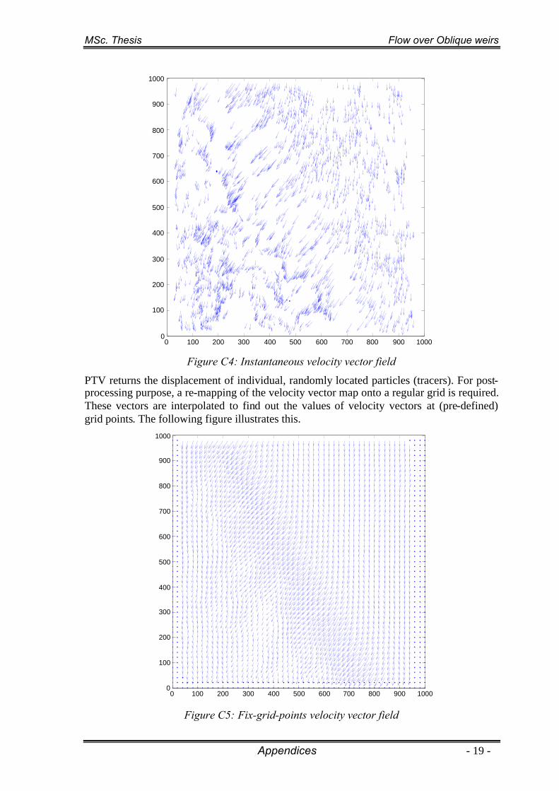
MSc. Thesis Flow over Oblique weirs
Appendices - 19 -
Figure C4: Instantaneous velocity vector field
PTV returns the displacement of individual, randomly located particles (tracers). For post-processing purpose, a re-mapping of the velocity vector map onto a regular grid is required.These vectors are interpolated to find out the values of velocity vectors at (pre-defined)grid points. The following figure illustrates this.
Figure C5: Fix-grid-points velocity vector field
0 100 200 300 400 500 600 700 800 900 10000
100
200
300
400
500
600
700
800
900
1000
0 100 200 300 400 500 600 700 800 900 10000
100
200
300
400
500
600
700
800
900
1000

MSc. Thesis Flow over Oblique weirs
- 20 - Appendices
Each couple of two consecutive images gives one instantaneous velocity vector field (fixedto a mesh grid as above). Finally the ensemble averaged (time-averaged) velocity vectorfield need to be calculated from these instantaneous ones.
C2. Analyses of the velocity vector fieldHaving the time-averaged velocity vector field, lots of underlying information related to thevelocities, the flow direction, and the flow pattern can be interpreted.
Taking one example from the test with the dike-form weir, =450, to illustrate these steps.Flow conditions: Q=35l/s, submerged flow. Main results will be visualized by mean offigures. The interpretation of each figure has been discussed in chapter 5. Hereafter thefigures aim at clarifying the purposes of appendix C.
0 0.5 1 1.5 20
0.2
0.4
0.6
0.8
1
1.2
1.4
1.6
1.8
2
Figure C6: Fix-grid-points, time-averaged velocity vector field
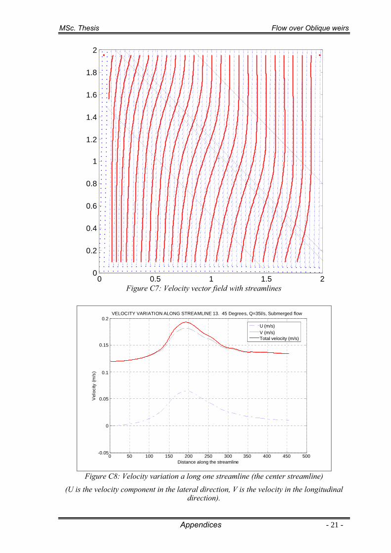
MSc. Thesis Flow over Oblique weirs
Appendices - 21 -
0 0.5 1 1.5 20
0.2
0.4
0.6
0.8
1
1.2
1.4
1.6
1.8
2
Figure C7: Velocity vector field with streamlines
0 50 100 150 200 250 300 350 400 450 500-0.05
0
0.05
0.1
0.15
0.2
Distance along the streamline
Vel
ocity
(m/s
)
VELOCITY VARIATION ALONG STREAMLINE 13. 45 Degrees, Q=35l/s, Submerged flow
U (m/s)V (m/s)Total velocity (m/s)
Figure C8: Velocity variation a long one streamline (the center streamline)
(U is the velocity component in the lateral direction, V is the velocity in the longitudinaldirection).

MSc. Thesis Flow over Oblique weirs
- 22 - Appendices
0 0.2 0.4 0.6 0.8 1 1.2 1.4 1.6 1.8 20
0.02
0.04
0.06
0.08
0.1
0.12
0.14
0.16
0.18
0.2
Lateral distance (m)
Ve
loc
ityc
omp
on
ent
norm
alt
oth
ew
eir
(m/s
)
VELO. VARIATION ALONG THE W.CREST 45 Degrees, Q=35l/s, Submerged flow
Figure C9: Variation of a velocity component a long the weir crest
(Used to calculate the discharge coefficient by integration)
0 0.5 1 1.5 2-0.1
-0.05
0
0.05
0.1
0.15
0.2
0.25
0.3
Distance from Right to Left (m)
U,
V,T
otal
velo
city
(m/s
)
FLOW VELOCITY DISTRIBUTION ACROSS THE FLUME. DOWNSTREAM OF WEIR, Q=30l/s, EMERGED FLOW
1.008 meter from the top
V (Velocity in the flow direction)U (Cross flow velocity)C (Total velocity)
Figure C10: Variation of different velocity components a long a cross-section
(This figure shows the asymmetry of the flow downstream of the weir. U is the velocitycomponent in the lateral direction, V is the velocity in the longitudinal direction).

MSc. Thesis Flow over Oblique weirs
Appendices - 23 -
0 0.5 1 1.5 2
0.5
1
1.5
2
0.12
0.13
0.14
0.15
0.16
0.17
0.18
Figure C11: Spatial distribution of the total velocity
0 1 2
0.5
1
1.5
2Longitudinal velocity component
-0.18
-0.16
-0.14
-0.12
0 1 2
0.5
1
1.5
2Crosssectional velocity component
-0.06
-0.05
-0.04-0.03
-0.02
-0.01
0 1 2
0.5
1
1.5
2Velocity component parallel to the weir
0.07
0.08
0.09
0.1
0.11
0.12
0 1 2
0.5
1
1.5
2Velocity component normal to the weir
0.1
0.12
0.14
0.16
Figure C12: Contours of different velocity components

MSc. Thesis Flow over Oblique weirs
- 24 - Appendices
0 0.5 1 1.5 20
0.2
0.4
0.6
0.8
1
1.2
1.4
1.6
1.8
245 Degrees, Q=35l/s, Submerged flow
Min Angle
Max Velocity
Oblique angle at center = 26.0695 0
Velocity at center = 0.18364m/sMin angle () = 24.99920
Max velocity = 0.1982m/s
26
28
30
32
34
36
38
40
42
44
Figure C13: Contours of the angle of obliqueness of the flow

MSc. Thesis Flow over Oblique weirs
Appendices - 25 -
APPENDIX D: MAJOR MATLAB SCRIPTS
During the course of this research, the Matlab scripts proved to be very useful andinevitable for the data processing and theory analysis. Some main scripts (in the form of*.m files) will be published hereafter for the purpose of further uses (reproduce the results,compare to others, or further investigate the topic). For a satisfactory usage of those scripts,the companion of other scripts as well as the data files are needed. Working with Matlab isof great weight for this study.
Beside Kadota’s PTV scripts that had been constructed, tested and used beforehand, theother Matlab *.m files were built on the demand of experiments and analysis with lots ofhelps from my colleagues. Most of the *.m files can run equally well in either Matlabversion 7.0 (R14) or Matlab version 6.5 environment. Only few of them need smallmodifications to be able to run in both environments due to differences in Matlab presetfunctions.
Some scripts can be widely applied for all the tests and cases, but formally each script isdedicated to one certain task and it should be modified upon certain case. With smallchanges to the inputs, outputs and structure, a single example from the scripts given belowcan be applied to other tests as well. The large number of experiments for PTV study (andthus great amount of data need to be analyzed) together with a wide range of interestedissues related to PTV analysis yield a large number of scripts. They can be found togetherwith measurement data in the attached DVD of this thesis.
Below is the list of scripts which will be presented, their application field (category), andshort descriptions about their function. The classification of scripts is only relative.
Table D1: List of presented Matlab scripts
No. File name Category Main function
1 theorymain.mTheory
research Finding/visualizing relations among Cd, Fr1 and S
2 theorypro.mTheory
research Solving equations from continuity, momentum balance and energy balance
3 ImportDataF.m ADV Import data from all experiments and call for PlotFigures.m
4 ADVmain3D.m ADV Import and convert data; Calculate and plot velocities
5 ADVpro.m ADV Perform calculation
6 PlotFigures.m ADV Calculation of all experiments and plot 3D-fig. of the flow
7 weirmain.m Weir formula Analysis of new weir discharge coefficient (Stelling definition)
8 weirpro.m Weir formula Perform the calculation
9 "KADOTA" PTV - data Comprise of sliding_image.m, corrimages_ptv_main.m, postproc.m
10 tuyen_calib.m PTV - data Calibrate the resulting UM, VM from Kadota analysis into appropriate values
11 calibratePTV.m PTV - data Perform the calibration (imitate the method of Breugem)
12 sline.m PTV - velocity Determine/plot streamlines over the existing vector field
13 extract1diagonal.m PTV - velocityExtract one velocity diagonal (along the crest of an oblique weir); calculate the
corrected discharge coefficient.14 extract1streamline.m PTV - velocity Extract velocity components along one stream line along the flow
15 extract1horizontal.m PTV - velocity Extract velocity values along one line (across the flume)
16 obliqueangle.m PTV - angle Calculate and quiver the oblique angle, velocity components
17 AnglePrediction.m PTV - angle Compare/plot theoretical values of the flow obl.angle against exp. results
18 AnglePrediction4560.m PTV - angle Determine the oblique angle of streamlines with different weir obl. angles

MSc. Thesis Flow over Oblique weirs
- 26 - Appendices
D.1. theorymain.mclear all;close all;clc;
%% RELATION S ~ Fr1h20 = .1;h2min = .05;h2max = .2;aweir = .104;Q = 40;
for i=1:5Q(i) = 15 + 5*i;[h1(i,:),Fr1(i,:),Fr2(i,:),S(i,:),Cd(i,:),H0(i,:),H2(i,:)] = theorypro(45,h2min,h2max,aweir,Q(i));
endH01=(3*sqrt(3)*Q./(2*sqrt(2)*2000*sqrt(9.81))).^(2/3);H0aweir=H01./aweir;
figure(1);hold on;plot(Fr1(1,:),H2(1,:)./H0(1,:),'b--','Linewidth',2)plot(Fr1(3,:),H2(3,:)./H0(3,:),'k-.','Linewidth',2)plot(Fr1(5,:),H2(5,:)./H0(5,:),'r-','Linewidth',2)grid onxlabel('Fr_1','Fontsize',14)ylabel('S','Fontsize',14)axis([0 1.2 0 1.2])legend(['Q = ',num2str(Q(1)),'l/s'],['Q = ',num2str(Q(3)),'l/s'],['Q = ',num2str(Q(5)),'l/s'],0);hold offset(gca,'Fontsize',14)
saveas(gcf,'S_Fr1','emf');
%% RELATION Cd ~ Ho/aweirH0re = H0./aweir; % Relatie upstream energy head% H0re (Q=20l/s)messdata1=[H0re(1,:)',Cd(1,:)'];sortdata1=sortrows(messdata1,1);sortdata1=sortdata1';% H0re (Q=30l/s)messdata3=[H0re(3,:)',Cd(3,:)'];sortdata3=sortrows(messdata3,1);sortdata3=sortdata3';% H0re (Q=40l/s)messdata5=[H0re(5,:)',Cd(5,:)'];sortdata5=sortrows(messdata5,1);sortdata5=sortdata5';
figure(2);set(0,'defaultaxesfontsize',14);plot(sortdata1(1,:),sortdata1(2,:),'b--','Linewidth',2);hold on; grid;plot(sortdata3(1,:),sortdata3(2,:),'k-.','Linewidth',2);plot(sortdata5(1,:),sortdata5(2,:),'r-','Linewidth',2);legend(['Q = ',num2str(Q(1)),'l/s'],['Q = ',num2str(Q(3)),'l/s'],['Q = ',num2str(Q(5)),'l/s'],0);xlabel('H_0/a_w (m)'); ylabel('C_d');saveas(gcf,'Cdv_H0re','emf');
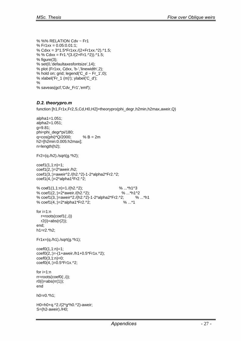
MSc. Thesis Flow over Oblique weirs
Appendices - 27 -
% %% RELATION Cdv ~ Fr1% Fr1xx = 0.05:0.01:1;% Cdxx = 3^1.5*Fr1xx./(2+Fr1xx.^2).^1.5;% % Cdxx = Fr1.*(3./(2+Fr1.^2)).^1.5;% figure(3);% set(0,'defaultaxesfontsize',14);% plot (Fr1xx, Cdxx, 'b-','linewidth',2);% hold on; grid; legend('C_d ~ Fr_1',0);% xlabel('Fr_1 (m)'); ylabel('C_d');%% saveas(gcf,'Cdv_Fr1','emf');
D.2. theorypro.mfunction [h1,Fr1x,Fr2,S,Cd,H0,H2]=theorypro(phi_degr,h2min,h2max,aweir,Q)
alpha1=1.051;alpha2=1.051;g=9.81;phi=phi_degr*pi/180;q=cos(phi)*Q/2000; % B = 2mh2=[h2min:0.005:h2max];n=length(h2);
Fr2=(q./h2)./sqrt(g.*h2);
coef1(1,1:n)=1;coef1(2,:)=2*aweir./h2;coef1(3,:)=aweir^2./(h2.^2)-1-2*alpha2*Fr2.^2;coef1(4,:)=2*alpha1*Fr2.^2;
% coef1(1,1:n)=1./(h2.^2); % ...*h1^3% coef1(2,:)=2*aweir./(h2.^2); % ...*h1^2% coef1(3,:)=aweir^2./(h2.^2)-1-2*alpha2*Fr2.^2; % ...*h1% coef1(4,:)=2*alpha1*Fr2.^2; % ...*1
for i=1:nr=roots(coef1(:,i))r2(i)=abs(r(2));
end;h1=r2.*h2;
Fr1x=(q./h1)./sqrt(g.*h1);
coef0(1,1:n)=1;coef0(2,:)=-(1+aweir./h1+0.5*Fr1x.^2);coef0(3,1:n)=0;coef0(4,:)=0.5*Fr1x.^2;
for i=1:nrr=roots(coef0(:,i));r0(i)=abs(rr(1));end
h0=r0.*h1;
H0=h0+q.^2./(2*g*h0.^2)-aweir;S=(h2-aweir)./H0;

MSc. Thesis Flow over Oblique weirs
- 28 - Appendices
H2=h2+q.^2./(2*g*h2.^2)-aweir;hd=h2-aweir;
Fr1=Fr1x; %.*(1+tan(phi)*h1./h0);Cd=q./((2/3)*H0.*sqrt((2/3)*g*H0));
D.3. ImportDataF.m% Import data for PlotFigures.m
close all;clear all;clc;fname = 'newADVmain3D.m';path2 = 'D:\MU - Lab\1.THESIS\ADV\60 DEGREES\Q40Un04Sep\';xx = [-200 -100 -40 20 30 40 60 80 100 200 400];
LL = length(xx);for i = 1 : LL
path = 'D:\MU - Lab\1.THESIS\ADV\60 DEGREES\Q40Un04Sep\'; % working directoryfolder = [path2 'x' num2str(xx(i))]cd(folder);newADVmain3D;
end;
cd(path2);
D.4. ADVmain3D.m%% READING AND CONVERTING ADV *.dat FILES TO *.mat FILES%% Nguyen Ba Tuyen
clc;close all;clear x y z U V W rotv roth A AA L L1 i TT phi velo;
freq = 25; % frequency of the ADV during measurements, Hzss = 70; % Signal strength (in counts), the value used for filterg = 9.81; % Gravitational accelerationaw = 10.4; % Weir height
% READING INPUT DATA FILESSSSpath = 'D:\MU - Lab\1.THESIS\ADV\60 DEGREES\Q40Un04Sep\x30\'; % workingdirectory[x,y,z,roth,rotv] = textread([path 'xyz30.txt']); % the file xyz.txt contains a list of measurementpoints (and viz. data files)depth = 13.39surfvelo = 0.343phi = 33.1TT = 6; % Test No.
% fname = ['D:\MU - Lab\1.THESIS\ADV\60 DEGREES\Q40Un04Sep\x60\' 'xyz60.txt']% fid = fopen(fname);% Measdata = textscan(fid, '%f %f %f %f %f');% M=cell2mat(Measdata)% fclose(fid);% x=M(:,1);% y=M(:,2);% z=M(:,3);

MSc. Thesis Flow over Oblique weirs
Appendices - 29 -
% roth=M(:,4);% rotv=M(:,5);
% PROCESSING DATAL1 = length(x)for i = 1:L1;
filein = [path, 'x', num2str(x(i)), 'y', num2str(y(i)), 'z', num2str(z(i)), '.dat']; % creating file-names[V(i),U(i),W(i),ust(i),vst(i),wst(i)] = ADVpro(filein, roth(i), rotv(i),ss);
end;
% Assign the new value for the point on bottom and point on the free surfacex=[x(1); x; x(1)];y=[y(1); y; y(1)];z=[0; z; depth];V=[0 V surfvelo*cos(pi*phi/180)]; % Note! V is the longitudinal velocity componentU=[0 U -surfvelo*sin(pi*phi/180)]; % U is the cross velocity componentW=[0 W 0]; % W is the vertical velocity component
velo = (U.^2+V.^2+W.^2).^(.5); % calculate the unified velocity% save ([path fileout],'x', 'y', 'z', 'U', 'V', 'W', 'ust', 'vst', 'wst') % save values in a *.mat file <--Cai nay co le cung can phai sua
% CALCULATE THE DEPTH-AVERAGED VELOCITY% surfvelo = 1.045*velo(length(velo));% "Intergration" - Method 2AA = 0; % total area of the vertical velocity profileL =length(velo) % last value, length of the velo matrixfor i=1 : (L-1);
A(i) = 1/2 * (velo(i) + velo(i+1)) * (z(i+1)-z(i)); % trapezoidals, and the last trapezoidal (nearbottom) is a triangular
AA = AA + A(i);end;
avevelo = AA/depth % Depth-averaged velocitydynH = avevelo^2/2/g % v2/2g (m)H = (depth/100 + dynH)*100 % Energy height (cm)
% VISUALIZE THE VELOCITY PROFILES%3D=================% draw streamlineplot3([-200 -50.4 -3.5 2.5 41.2 100 400],[20 20 1.2 -1.5 -25 -40 -50],[0 0 aw aw 0 0 0],'r-.','linewidth',1);hold on;% draw bottom & weirplot3([-200 400 400 -200 -200],[20 20 -50 -50 20],[0 0 0 0 0],'linewidth',1); % this is the bottomplot3([-50.4 29.6 39.6 119.6 1.6 -81.6 -91.6 -171.6 -50.4],[20 20 20 20 -50 -50 -50 -50 20],[0 aw aw0 0 aw aw 0 0],'linewidth',1); % this is the side wall of the weirplot3([29.6 -91.6],[20 -50],[aw aw],'linewidth',1); % this is the weir upstream crestplot3([39.6 -81.6],[20 -50],[aw aw],'linewidth',1); % this is the weir downstream crest
% draw vectorsquiver3(x',y',z',V*50,U*50,W*50);% draw vertical base lineplot3([x(1) x(L)],[y(1) y(L)],[z(2)-0.5 z(L)],'k');axis equal;% axis([0 100 -50 20 0 20]) % axis restriction

MSc. Thesis Flow over Oblique weirs
- 30 - Appendices
grid;
% %2D=================% % draw bottom & weir% plot([-200 -50.4 -3.5 2.5 41.2 200],[0 0 10.4 10.4 0 0]);% hold on;% % draw vectors% quiver(x',z',V*100,W*100);% % draw vertical base line% plot([x(1) x(L)],[z(2)-0.5 z(L)],'k');% axis equal;% axis([0 100 0 20]) % axis restriction% grid;
title('ADV MEASUREMENT');xlabel('Longitudinal distance (cm)');ylabel('Depth (cm)');
% Save data to use later ("fin" = final)% (the colon notation (:) cannot be used here because of assignment dimension mismatch.for i = 1: L
xfin(TT,i)=x(i);yfin(TT,i)=y(i);zfin(TT,i)=z(i);Vfin(TT,i)=V(i);Ufin(TT,i)=U(i);Wfin(TT,i)=W(i);
end;depthfin(TT)=depth;avevelofin(TT)=avevelo;
D.5. ADVpro.mfunction [U,V,W,ust,vst,wst] = ADVpro(filein, roth, rotv,ss)
%% Reading ADV data file (*.dat)[t1,gar,velx,vely,velz,velz2,amp1,amp2,amp3,amp4,snr1,snr2,snr3,snr4,cor1,cor2,cor3,cor4] =...
textread(filein,'%f%8s%f%f%f%f%f%f%f%f%f%f%f%f%f%f%f%f');
roth = roth*pi/180;rotv = rotv*pi/180;
t = (t1-t1(1))/25; % Time steps, subtract the first time step because all the time steps start at avalue <> 0, then divides by freq.
% Filterif ss > 0
range = find(amp1 >= ss & amp2 >= ss & amp3 >= ss & amp4 >= ss);u1 = velx(range); v1 = vely(range); w1 = velz(range); t = t(range);
elseu1 = velx; v1 = vely; w1 = velz;
end;
% u1 = velx; v1 = vely; w1 = velz;
%% Rotation of velocity vectorsux = (u1.*cos(rotv) - w1.*sin(rotv)).*cos(roth) + v1.*sin(roth);vy =-(u1.*cos(rotv) - w1.*sin(rotv)).*sin(roth) + v1.*cos(roth);

MSc. Thesis Flow over Oblique weirs
Appendices - 31 -
wz = u1 .*sin(rotv) + w1.*cos(rotv);
%% Average velocitiesU = mean(ux);V = mean(vy);W = mean(wz);
% % Calculating turbulence stresses% % Standaard deviation of velocities% ust = std(ux);% vst = std(vy);% wst = std(wz);%% % Creation of turbulente velocity vectors% ua = ux - mean(ux);% va = vy - mean(vy);% wa = wz - mean(wz);
D.6. PlotFigures.m%% NOTE!%% LET OP!%% in order to run this script, you must run ImportDataF.m to import data from all smallmeasurement at each%% measurement point on the plan view (modify & run ImportDataF.m)%% or you need to import xfin, yfin, zfin, Ufin, Vfin, Wfin%% from associated excel file.
clc;close all;
% clear x y z U V W rotv roth A AA L L1 i TT phi velo;
[L2 L] = size(xfin);
%VISUALIZE THE VELOCITY PROFILESfigure(1);hold on;set(0,'defaultaxesfontsize',14);set(0,'DefaultTextfontSize',14);%3D=================================% draw streamlineplot3([-200 -50.4 -3.5 2.5 41.2 100 400],[20 20 1.2 -1.5 -25 -40 -50],[0 0 aw aw 0 0 0],'r-.','linewidth',2);% draw water surfaceplot3([-200 -100 -40 0 20 30 40 60 80 100 200 400],[20 20 16 0 -12 -18 -25 -30 -35 -40 -42 -50],[14.18 14.45 13.94 13.55 13.55 13.39 13.61 14.03 14.16 14.24 14.26
14.28],'m-','linewidth',1);% draw bottom & weir% plot3([119.6 400 400 -200 -200 -50.4],[20 20 -50 -50 20 20],[0 0 0 0 0 0],'linewidth',2); % this isthe bottomplot3([-50.4 119.6],[20 20],[0 0],'b--','linewidth',1); % this is the bottom shaded lineplot3([400 400 -200 -200 -50.4],[20 -50 -50 20 20],[0 0 0 0 0],'linewidth',2); % this is the bottom
plot3([-50.4 29.6 39.6 119.6 1.6 -81.6 -91.6 -171.6 -50.4],[20 20 20 20 -50 -50 -50 -50 20],[0 aw aw0 0 aw aw 0 0],'linewidth',2); % this is the side wall of the weirplot3([29.6 -91.6],[20 -50],[aw aw],'linewidth',2); % this is the weir upstream crestplot3([39.6 -81.6],[20 -50],[aw aw],'linewidth',2); % this is the weir downstream crest% draw vectorsquiver3(xfin,yfin,zfin,Vfin,Ufin,Wfin,0.3);

MSc. Thesis Flow over Oblique weirs
- 32 - Appendices
% draw vertical base linesfor i = 1:L2
plot3([xfin(i,1) xfin(i,1)],[yfin(i,1) yfin(i,1)],[zfin(i,1)-1 depthfin(i)],'k');end;axis equal;axis([-50 120 -50 20 0 20]) % axis restrictiongrid;title('ADV MEASUREMENT');xlabel('Longitudinal distance (cm)');ylabel('Depth (cm)');
saveas(gcf,'VeloPro3D','emf');
%2D=================================figure(2);hold on;% draw water surfaceplot([-200 -100 -40 0 20 30 40 60 80 100 200 400],[14.1814.45 13.94 13.55 13.55 13.39
13.61 14.03 14.16 14.24 14.26 14.28],'m-','linewidth',1);% draw bottom & weirplot([-200 400],[0 0]);plot([-200 -50.4 -3.5 2.5 41.2 400],[0 0 10.4 10.4 0 0]);% draw vectorsquiver(xfin,zfin,Vfin,Wfin,0.3);% % draw vertical base line% for i = 1 : L2% line([xfin(i,1) xfin(i,1)],[zfin(i,1)-1 depthfin(i)],'LineWidth',1,'Color','k');% end;axis equal;axis([-50 120 -5 25]) % axis restrictiongrid;title('ADV MEASUREMENT');xlabel('Longitudinal distance (cm)');ylabel('Depth (cm)');set(0,'defaultaxesfontsize',14);set(0,'DefaultTextfontSize',14);saveas(gcf,'VeloProVW','emf');
figure(3);hold on;% draw water surfaceplot([-200 -100 -40 0 20 30 40 60 80 100 200 400],[14.1814.45 13.94 13.55 13.55 13.39
13.61 14.03 14.16 14.24 14.26 14.28],'m-','linewidth',1);% draw bottom & weirplot([-200 400],[0 0]);plot([-200 -50.4 -3.5 2.5 41.2 400],[0 0 10.4 10.4 0 0]);% draw vectorsquiver(xfin,zfin,Ufin,Wfin,0.3);% draw vertical base linefor i = 1 : L2
line([xfin(i,1) xfin(i,1)],[zfin(i,2)-1 zfin(i,L)],'LineWidth',1,'Color','k');end;axis equal;axis([-50 120 -5 25]) % axis restrictiongrid;title('ADV MEASUREMENT');xlabel('Longitudinal distance (cm)');ylabel('Depth (cm)');

MSc. Thesis Flow over Oblique weirs
Appendices - 33 -
set(0,'defaultaxesfontsize',14);set(0,'DefaultTextfontSize',14);saveas(gcf,'VeloProUW','emf');
D.7. weirmain.m%% THEORETICAL ANALYSIS OF WEIR "DISCHARGE COEFFICIENT"%% Imitate the subroutine of Prof. G.S.Stelling
close all;clear all;clc;
wheight = 0.104; % Weir height [m]headloss = 7.5*10^(-5) % Headloss due to bottom friction (Measured value, = 0.3mm);% headloss = 0;
% IMPORT EXPERIMENT DATA FROM FILEmeas=importdata(['D:\MU - Lab\1.THESIS\Matlab works\weirsubroutine\expdata.txt'],' \t');X_meas=getfield(meas,'data');%Read variablesqE=X_meas(:,3); % Specific discharge, "E" stands for "Experimental"zuE=X_meas(:,5); % Upstream water levelzcE=X_meas(:,6); % Crest water levelzdE=X_meas(:,8)+headloss; % Downstream water level; + Head loss due to bottom frictionFrcE=X_meas(:,9); % Froude number on top of the weirSE=X_meas(:,10); % Submergence
% MAIN CALCULATIONL = length(qE);for i=1:L
zu(i)=zuE(i);zd(i)=zdE(i);aw(i)=wheight;
[zcCrit(i),zdTrans(i),zc(i),q(i),uu(i),uc(i),ud(i),zcEmp(i),qEmp(i),qEmpT(i)]=weirpro(zu(i),zd(i),aw(i));Cd(i) = qE(i)/q(i); % New definition of the Discharge Coefficient, solved analyticallyCdEmp(i) = qE(i)/qEmp(i); % New definition of the Discharge Coefficient, solved empirically
(Stelling)CdEmpT(i)= qE(i)/qEmpT(i); % Correction by Tuyen.Rq(i)=Cd(i)/CdEmp(i);RqT(i)=Cd(i)/CdEmpT(i);Rzc(i)=zc(i)/zcEmp(i);
end;
p=7;x=0.1:0.01:0.99;y=(1-x.^p).^0.04;
% EXPORT RESULTSfigure(1);set(gcf,'OuterPosition',[100 100 920 640]);hold on;set(0,'defaultaxesfontsize',14);set(0,'DefaultTextfontSize',14);plot(SE,Cd,'b+');plot(SE,CdEmp,'ro');% plot(x,y,'g-');

MSc. Thesis Flow over Oblique weirs
- 34 - Appendices
plot(SE,Rq,'bx');plot(SE,RqT,'k.');plot(SE,Rzc,'m.');axis equal;axis([0 1.2 0 1.2]) % axis restrictiongrid;title('REDUCTION FACTOR (Cd) ~ SUBMERGENCE (S)');legend('Cd=q_e_x_p/q_a_n_a (analytical)','Cd=q_e_x_p/q_e_m_p (empirical,Stelling)','Rq=q_a_n_a/q_e_m_p (Stelling)','Rq (Tuyen)','Rzc=zc_a_n_a/zc_e_m_p',0);xlabel('Submergence (-)');ylabel('Ratio (-)');saveas(gcf,'Cd_S','emf');
figure(2);set(gcf,'OuterPosition',[100 100 920 640]);hold on;plot(SE,Rq,'bo');plot(SE,RqT,'kh');plot(SE,Rzc,'^r');axis equal;axis([0.6 1 0.8 1.1]) % axis restrictiongrid;% title('REDUCTION FACTOR FOR SPECIFIC DISCHARGE');legend('R_q=q_c_o_m_p/q_e_m_p (Stelling)','R_q=K_q*(q_c_o_m_p/q_e_m_p)(Tuyen)','R_h_1=h1_c_o_m_p/h1_e_m_p',0);xlabel('Submergence (-)');ylabel('Ratio (-)');plot([0 1],[1 1],'k--');saveas(gcf,'Rq','emf');
figure(3);set(gcf,'OuterPosition',[100 100 920 640]);hold on;set(0,'defaultaxesfontsize',14);set(0,'DefaultTextfontSize',14);plot(FrcE,Cd,'b+');plot(FrcE,CdEmp,'ro');plot(FrcE,Rq,'k*');plot(FrcE,Rzc,'m.');axis equal;axis([0 1 0.2 1.1]) % axis restrictiongrid;title('REDUCTION FACTOR (Cd) ~ FROUDE NUMBER (Fr_crest)');legend('C_d_(_R_)=q_e_x_p/q_c_o_m_p (complex)','C_d_(_R_)=q_e_x_p/q_e_m_p(empirical)','R_q=q_c_o_m_p/q_e_m_p','R_h_1=h1_c_o_m_p/h1_e_m_p',0);xlabel('Froude number at weir crest (-)');ylabel('Ratio (-)');saveas(gcf,'Cd_Frc','emf');
figure(4);set(gcf,'OuterPosition',[100 100 920 640]);hold on;set(0,'defaultaxesfontsize',14);set(0,'DefaultTextfontSize',14);plot(SE,Rq,'bo');plot(x,y,'k--');axis equal;axis([0.4 1 0.8 1.1]) % axis restrictiongrid;% title('MODIFICATION BY TUYEN');

MSc. Thesis Flow over Oblique weirs
Appendices - 35 -
legend('Rq=q_a_n_a/q_e_m_p (Stelling)','C_q=f(S) (Tuyen)',0);xlabel('Submergence (-)');ylabel('r (-)');saveas(gcf,'R','emf');
D.8. weirpro.m%% Perform the calculation (solving equations, finding roots of%% polinomials...) based on Energy conservation and Momentum conservation
function [zcCrit,zdTrans,zc,q,uu,uc,ud,zcEmp,qEmp,qEmpT]=weirpro(zu,zd,aw)
% Input Variables (3)% zu : upstream water level [m]% zd : downstream water level [m]% aw : weir height [m]
% Output Variables (10)% zc : waterlevel on crest [m]% zcCrit : waterlevel on crest for critical flow (perfect weir) [m]% zdTrans : transition down stream waterlevel (from emerged to submerged flow, and viceversa) [m]% q : specific discharge (= total discharge/m) [m2/s]% uu : upstream velocity [m/s]% uc : velocity on crest [m/s]% ud : downstream velocity [m/s]% zcEmp : waterl level on crest, calculated by the empirical formula of Stelling [m]% qEmp : specific discharge, calculated from zcEmp% qEmpT : specific discharge, calculated from zcEmp, with a correction factor from Tuyen
g=9.81;h1=zu+aw;
% Compute critical depth on crest by solving: z^3 - 3*h1^2*z + 2*h1^2*Zu=0% equation is solved analytically method of Cardanocoef1(1) = 1;coef1(2) = 0;coef1(3) = -3*h1^2;coef1(4) = 2*h1^2*zu;
rr1=roots(coef1(:));zcCrit=abs(rr1(3));h2Crit=zcCrit+aw;u2Crit=sqrt(g*zcCrit);qCrit=zcCrit*u2Crit;
% Compute the transition downstream water level ZdTrans% for this the equation F=q^2/h3+0.5*g*h3^2 is solved analytically with Cardano methodcoef2(1) = 1;coef2(2) = 0;coef2(3) = -(2*qCrit*u2Crit/g + h2Crit^2);coef2(4) = 2*qCrit^2/g;
rr2=roots(coef2(:));h3Trans=abs(rr2(2));zdTrans=h3Trans-aw;
% MAIN CALCULATION% Check zd% Compute the water level on crest (zc) for different flow regimes
MSc. Thesis Flow over Oblique weirs
- 36 - Appendices
h3=zd+aw;h1=zu+aw;if (zd<=zdTrans)
zc = zcCrit;q = qCrit;zcEmp = zcCrit; % Zc calculated by the empirical formula of
StellingqEmp = qCrit;qEmpT = qCrit;
else% [qsub,zcsub]=solve('q^2/2/g*(1/zu^2-1/zc^2)+(zu-zc)','q^2*(1/zc-1/h3)+g/2*((zc+aw)^2-h3^2)');% q=qsub;% zc=zcsub;
fzc = @(zc) 4*h1^2*zc*(zc-zu)*(h3-zc)-h3*(h3^2-(zc+aw)^2)*(zc^2-h1^2);zc=fzero(fzc,zu); % Zc solved analytically by trials, solution found
near "zu"q=abs(sqrt(2*g*(zc-zu)*h1^2*zc^2/(zc^2-h1^2)));zcEmp=zcCrit+((zd-zdTrans)/(zu-zdTrans))*(zu-zcCrit); % Zc calculated by the empirical
formula of Stelling (Empirical)qEmp=abs(sqrt(2*g*(zcEmp-zu)*h1^2*zcEmp^2/(zcEmp^2-h1^2))); % Solved analytically from
zcEmpqEmpT=abs(sqrt(2*g*(zcEmp-zu)*h1^2*zcEmp^2/(zcEmp^2-h1^2)))/(1-(zd/zu)^7)^(1/30); %
correction by Tuyen% T=solve('4*h1^2*zc*(zc-zu)*(h3-zc)-h3*(h3^2-(zc+aw)^2)*(zc^2-h1^2)',zc) % Try ananalytical formula (Tuyen)end;
uu=q/h1;uc=q/zc;ud=q/h3;
D.9. tuyen_calib.m%% TUYEN - Calibration for the flume%% to calibrate the UM, VM in to right values
% Input parameters: UM(51x51), VM(51x51), XI, YI, CalibMatrix% Output parameters: UM(51x51), VM(51x51), XIn, YIn% Temporary parameters: UM1(2061,1), VM1(2061,1), XI1, XI1% UM2(2061,1), VM2(2061,1), YI2, YI2
close all;clear UM1 VM1 XI1 YI1;CalibMatrix = [491.341 1008 431.526 1018 14.7836 0.453107 -1.72075
4.25677 4.87093 -0.0599318 0.0188008 -3.26483 -0.113468 3.5333 12.4701 -4.39329 -0.211976 0.0339166 1.42651
-3.92475 3.79122 -1.87388 3.25923 0.0409122];CalibMatrix = CalibMatrix';le=length(UM);L=le*le;
for i = 1:lefor j = 1:leUM1((i-1)*le+j) = UM(i,j);VM1((i-1)*le+j) = VM(i,j);XI1((i-1)*le+j) = XI(i,j);YI1((i-1)*le+j) = YI(i,j);end;

MSc. Thesis Flow over Oblique weirs
Appendices - 37 -
end;
oldparas = [XI1' YI1' UM1' VM1'];newparas = calibratePTV(oldparas, CalibMatrix);XI2=(newparas(:,1))';YI2=(newparas(:,2))';UM2=(newparas(:,3))';VM2=(newparas(:,4))';
for i = 1:lefor j = 1:leXIn(i,j) = XI2((i-1)*le+j);YIn(i,j) = YI2((i-1)*le+j);UMn(i,j) = UM2((i-1)*le+j);VMn(i,j) = VM2((i-1)*le+j);end;
end;
% Calibrationcalib1 = 0.0605; % The calibration factor (to convert the velocity from pixel/frame -->>meter/second)calib2 = 0.002016; % The calibration factor (to convert the distance from pixel -->> meter)UMn =UMn.*calib1;VMn =VMn.*calib1;XIn =XIn.*calib2;YIn =YIn.*calib2;
% Interpolation vectors at fix grid points
% [xn, yn]=meshgrid(0:20:1000, 0:20:1000);% UMgr = interp2(XI,YI,UM,xn,yn);% VMgr = interp2(XI,YI,VM,xn,yn);
% [xn, yn]=meshgrid(0:20:1000, 0:20:1000);% UMgr = interp2(xn,yn,UM,XI,YI);% VMgr = interp2(xn,yn,VM,XI,YI);
figure(1);set(gcf,'OuterPosition',[0 100 1020 740]);quiver(XIn,YIn,UMn,VMn,0.8);axis equal; axis([0 2 0 2]);hold on;ch3=' 45 Degrees, Q=35l/s, Submerged flow';set(0,'defaultaxesfontsize',14);title(ch3);[offset,a,b,cenpointx,cenpointy]=plotweir45('k',1); % Plot the plain view of the oblique weir
% EXPORT FIGUREsaveas(gcf,'vecfield','emf');
D.10. calibratePTV.mfunction newPTV=calibratePTV(oudPTV, IcPar)%oudPTV is a matrix with [xi yi Dxi Dyi], where xi is the x loaction of%particle number i, yi its y location (both in pixels). Dxi is the%displacement of particle i in the x direction in pixels/frame, Dyi is the%dispalcement in y direction
s = 2.*(oudPTV(:,1)-IcPar(1))./IcPar(2);%centreren data

MSc. Thesis Flow over Oblique weirs
- 38 - Appendices
t = 2.*(oudPTV(:,2)-IcPar(3))./IcPar(4);
dx = IcPar(5)+ IcPar(6).*s + IcPar(7).*s.*s + IcPar(8).*s.*s.*s + IcPar(9).*t + IcPar(10).*t.*t +IcPar(11).*t.*t.*t + IcPar(12).*s.*t + IcPar(13).*s.*s.*t+IcPar(14).*s.*t.*t;
dy = IcPar(15)+ IcPar(16).*s + IcPar(17).*s.*s + IcPar(18).*s.*s.*s + IcPar(19).*t + IcPar(20).*t.*t+ IcPar(21).*t.*t.*t + IcPar(22).*s.*t + IcPar(23).*s.*s.*t+IcPar(24).*s.*t.*t;
newPTV(:,1) = oudPTV(:,1) + dx;newPTV(:,2) = oudPTV(:,2) + dy;
xeind=oudPTV(:,1)+oudPTV(:,3);yeind=oudPTV(:,2)+oudPTV(:,4);
s = 2.*(xeind-IcPar(1))./IcPar(2);%centreren datat = 2.*(yeind-IcPar(3))./IcPar(4);
dx2 = IcPar(5)+ IcPar(6).*s + IcPar(7).*s.*s + IcPar(8).*s.*s.*s + IcPar(9).*t + IcPar(10).*t.*t +IcPar(11).*t.*t.*t + IcPar(12).*s.*t + IcPar(13).*s.*s.*t+IcPar(14).*s.*t.*t;
dy2= IcPar(15)+ IcPar(16).*s + IcPar(17).*s.*s + IcPar(18).*s.*s.*s + IcPar(19).*t + IcPar(20).*t.*t+ IcPar(21).*t.*t.*t + IcPar(22).*s.*t + IcPar(23).*s.*s.*t+IcPar(24).*s.*t.*t;
%extradisp = [dx-dx2 dy-dy2];
xeindnew = xeind+dx2;yeindnew = yeind+dy2;
%snelheid bepalen uit beide nieuwe puntennewPTV(:,3)=xeindnew-newPTV(:,1);newPTV(:,4)=yeindnew-newPTV(:,2);
return;
D.11. sline.m%% Draw streamlines over the existing vector field%% Parameters depends on flow regimes, discharge...%% Please import data from file "ser_aa_im.mat" before run this script
dx=40; % distance between two adjacent streamlinesy1=970; % starting value of ycalib1 = 0.0605; % The calibration factor (to convert the velocity from pixel/frame -->>meter/second)calib2 = 0.002016; % The calibration factor (to convert the distance from pixel -->> meter)close all;
figure(1);set(gcf,'OuterPosition',[0 100 1020 740]);quiver(XIn,YIn,UMn,VMn,2); % After calibrationaxis equal;hold on;
% Draw streamlines (upstream & right handside of the flume)startx=[20:dx:1000]; startx=startx.*calib2;starty(1:length(startx))=y1*calib2;sl=streamline(XIn,YIn,UMn,VMn,startx,starty);set(sl,'color','r','linewidth',2);
%==========================================================================% DRAW 60o WEIR'S PLAN VIEW FROM REAL IMAGE:
MSc. Thesis Flow over Oblique weirs
Appendices - 39 -
% offset di 1 doan 20pix theo huong 45 do (Northwest) -> Dx = +28, Dy = +28offset = 28; %(=20*sqrt(2))
psizex=1008; psizey=1018;% Center line% a=[230+offset 810+offset]; a=a.*calib2;% b=[psizey+offset 0+offset]; b=b.*calib2;% plot(a,b,'color','w','linewidth',1);% two crest linesa=[210+offset 799+offset 831+offset 242+offset]; a=a.*calib2;b=[psizey+offset 0+offset 0+offset psizey+offset]; b=b.*calib2;plot(a,b,'color','k','linewidth',1);% downstream linea=[16+offset 555+offset]; a=a.*calib2;b=[(psizey-80)+offset 0+offset]; b=b.*calib2;plot(a,b,'color','k','linewidth',1);% upstream linea=[480+offset psizex+offset]; a=a.*calib2;b=[psizey+offset (psizey-900)+offset]; b=b.*calib2;plot(a,b,'color','k','linewidth',1);% Center pointcenpointx = (510+offset)*calib2;cenpointy = (492+offset)*calib2;plot(cenpointx, cenpointy,'k*');%==========================================================================
set(0,'defaultaxesfontsize',14);title(ch3);
% EXPORT FIGUREsaveas(gcf,'stlines','emf');
D.12. extract1diagonal.m%% Extracting 1 diagonal U(51) from UM(51x51); and V(51) form VM(51x51)%% Calculating the projected (specific) discharge coefficient from PTV%% measurement, comparing with point-gauge measured Cd%% Compose vector C (total velocity) from vectors U and V
close all; clc;
calib1 = 0.0605; % The calibration factor (to convert the velocity from pixel/frame -->>meter/second)calib2 = 0.002016; % The calibration factor (to convert the distance from pixel -->> meter)psizex=1008;psizey=1018;offset = 15; %(=20*sqrt(2))
figure(1);set(gcf,'OuterPosition',[0 0 1000 740]);quiver(XIn,YIn,UMn,VMn,2); % After calibrationaxis equal;hold on;% Draw streamlines (upstream & right handside of the flume)startx=[20:dx:1000]; startx=startx.*calib2;starty(1:length(startx))=y1*calib2;sl=streamline(XIn,YIn,UMn,VMn,startx,starty);set(sl,'color','r','linewidth',2);set(0,'defaultaxesfontsize',14);
MSc. Thesis Flow over Oblique weirs
- 40 - Appendices
title(ch3);
% Plot the plain view of the oblique weir[offset,a,b,cenpointx,cenpointy]=plotweir45('k ',1);plot(a,b,'g--','linewidth',2);
XX=[50:9.7:1020]; XXn = XX.*calib2; % Coordinate of extracted points along weircenter lineYY=[1030:-9.9:40]; YYn = YY.*calib2; % (Toa do cac diem trich xuat van toc doctheo duong cheo tim dap)deltaXX = 9.7*calib2;% deltaYY = 9.9*calib2;plot(XXn,YYn,'r+');
% CALCULATE THE OBLIQUE ANGLE AND VELOCITY COMPONENTS[s1, s2] = size(UMn);for i = 1:s1
for j = 1:s2MoArad(i,j) = atan(UMn(i,j)/VMn(i,j))+(pi/4); % Angle in radian. MoA = Matrix of AnglesMoA(i,j) = 180/pi*MoArad(i,j); % Oblique angletotalV(i,j)=(UMn(i,j)^2+VMn(i,j)^2)^0.5; % Total velocityVP(i,j) = totalV(i,j)*sin(MoArad(i,j)); % Velocity component perpendicular to the long
axis of the weir crestVL(i,j) = totalV(i,j)*cos(MoArad(i,j)); % Velocity component parallel to the long axis of
the weir crestend;
end;
VPXX = interp2(XI,YI,VP,XX,YY); % velocity component normal to the weir crest(at extreacted points)
Lweir = 2/cos(pi/4) % length of the weirdataVPall = find(isnan(VPXX)==0); % find the points with valid dataLall = (length(dataVPall) - 1)*9.7*calib2; Lall = Lall/cos(pi/4) % portion of the weir withvalid datadataVPhalf = find(XXn>0.5&XXn<1.5); % consider 1m wide in the middle of theflumeLhalf = (length(dataVPhalf) - 0)*9.7*calib2; Lhalf = Lhalf/cos(pi/4) % length of the middlepart (=1m/cos45)
% It's a pitty the result form PTV vector field doesn't cover the whole% length of the weir. So we will consider the portion of the total% discharge which flow through this part only (evaluated value, not% absolute realistic)
h1 = 0.085; % water depth above the weir, mQ1tot = 0.03; % Total discharge, m3/s (=30l/s)Q1por = Q1tot * Lall/Lweir % Considered discharge, only a portion, m3/s
% FIGURE 2 ======================figure(2);set(gcf,'OuterPosition',[0 0 1020 740]);plot(XXn,VPXX,'b--','linewidth',1); hold on; grid; % Plot all the data of VP along weir centerline
MSc. Thesis Flow over Oblique weirs
Appendices - 41 -
% plot(XXn(dataVPall),VPXX(dataVPall),'b --','linewidth',1) % Plot all the data of VP along weircenter line (same)plot(XXn(dataVPhalf),VPXX(dataVPhalf),'r-','linewidth',2) % Plot all the data of VP along weircenter line (only 1m wide)plot([0.5 0.5],[0 VPXX(dataVPhalf(1))],'k--');plot([1.5 1.5],[0 VPXX(dataVPhalf(length(dataVPhalf)))],'k--');fill(1,0.1,'y');
axis([0 2 0 .2]);xlabel('Lateral distance (m)'); ylabel('Velocity component normal to the weir (m/s)');title(['VELO. VARIATION ALONG THE W.CREST ', ch3]);saveas(gcf,'dischpor','emf');
Qall = trapz(VPXX(dataVPall)) * deltaXX * h1 % Discharge value (over the portion with validdata) calculated from velocity profileQhalf = trapz(VPXX(dataVPhalf)) * deltaXX * h1 % Discharge value (over 1m wide) calculatedfrom velocity profile
Qhalfcal = Q1por * (Qhalf/Qall)Rq=Qhalfcal/Q1tot
% plot(x,U,'b-.','linewidth',1); hold on; grid;% plot(x,V,'k--','linewidth',1);% plot(x,C,'r','linewidth',2);%% set(0,'defaultaxesfontsize',14);% legend('U (m/s)','V (m/s)','Total velocity (m/s)',0);
D.13. extract1streamline.m%% Extracting & plotting 1 stream line along the flow%% -->> 1 matrix with 2 collums, contains x & y co-ordinates of the points along 1 streamline%% Input = streamline number (from left)%% grid size, starting point
%% Please run "sline.m" before run this script
close all; clc;
% INPUT DIMENSIONS IN PIXELS:strno =13; % The 13th streamline from the left.ch =num2str(strno);picsize =1000; % Size of image (1000x1000 pixels).grsize =20; % Resolution of the velocity vector field (grid size)y1 = 970;calib1 = 0.0605; % The calibration factor (to convert the velocity from pixel/frame -->>meter/second)calib2 = 0.002016; % The calibration factor (to convert the distance from pixel -->> meter)
% RE-DRAW THE VECTOR-FIELD AND DRAW STREAMLINES (upstream & right handside of theflume)% quiver(XI,YI,UM,VM,2);% axis equal;% startx=[20:grsize:picsize];% starty(1:length(startx))=y1;% sl=streamline(XI,YI,UM,VM,startx,starty);% set(sl,'color','r','linewidth',2);% pause(1);

MSc. Thesis Flow over Oblique weirs
- 42 - Appendices
% extract co-ordinates of one streamline into matrix Astline =stream2(XIn,YIn,UMn,VMn,startx,starty);A =stline{strno};L= length(A(:,1));
k1=0:20:picsize; k1=k1.*calib2;k2=0:20:picsize; k2=k2.*calib2;b1=A(:,1); b2=A(:,2);
% k1=0:20:picsize;% k2=0:20:picsize;% b1=A(:,1)./calib2; b2=A(:,2)./calib2;b1(isnan(b1))=[]; b2(isnan(b2))=[];
UL=-interp2(k1,k2,UMn,b1,b2); % Interpolate UL (1 array) from UM (1 matrix)VL=-interp2(k1,k2,VMn,b1,b2);CL=(UL.^2 + VL.^2).^0.5; CL(isnan(VL))=[];
% xdistance(1) =0;% for j=2:L% xdistance(j) = xdistance(j-1) + ((A(j,1)-A(j-1,1))^2 + (A(j,1)-A(j-1,1))^2)^0.5;% end;%% for i = 1:L% Ugr(i,1) =UL(i); Ugr(i,2) =xdistance(i);% Vgr(i,1) =VL(i); Vgr(i,2) =xdistance(i);% Cgr(i,1) =CL(i); Cgr(i,2) =xdistance(i);% end;%% plot(Ugr,'b-.','linewidth',1); hold on; grid; pause(1);% plot(Vgr,'k--','linewidth',1); pause(1);% plot(Cgr,'r','linewidth',2);
plot(UL,'b-.','linewidth',1); hold on; grid;plot(VL,'k--','linewidth',1);plot(CL,'r','linewidth',2);
set(0,'defaultaxesfontsize',14);legend('U (m/s)','V (m/s)','Total velocity (m/s)',0);xlabel('Distance along the streamline'); ylabel('Velocity (m/s)');grtitle = ['VELOCITY VARIATION ALONG STREAMLINE ', ch,'.', ch3]; title(grtitle);
saveas(gcf,['stl',num2str(strno)],'emf');
D.14. extract1horizontal.m%% Extract velocity values along a line (across the flume)%% Draw U, V and C=sqrt(U^2 + V^2) | ^ VM% | |% | Flow |% V |-----> UM%
clf; clc;clear UM1 VM1 U V C x;% (XI YI UM VM) = importdata('ser_aa_im');
calib = 0.0605; % The calibration factor (to convert the velocity from pixel/frame -->>meter/second)

MSc. Thesis Flow over Oblique weirs
Appendices - 43 -
calib2 = 0.002016; % The calibration factor (to convert the distance from pixel -->> meter)
i=30; % Extract vector along the line across the flume (i*20 pixels from top of the picture)dist = (i*20)*calib2;
n=length(UMn);for j=1:n
U(j)=-UMn(i,j);V(j)=-VMn(i,j);C(j)=sqrt(U(j)^2+V(j)^2);x(j)=j*calib2*20;
end% U) <---| |% | |% | | Flow% (V) V V
% Plotingline1=plot(x,V,'k--'); hold on; grid;line2=plot(x,U,'b-.');line3=plot(x,C);set(line3,'color','r','linewidth',2);
v=axis; axis([0 2 v(3) v(4)]); % x-Axis restricted to 0 -> 2 (m)xlabel('Distance from Right to Left (m)'); ylabel('U, V, Total velocity (m/s)');legend('V (Velocity in the flow direction)', 'U (Cross flow velocity)', 'C (Total velocity)',0);title(['FLOW VELOCITY DISTRIBUTION ACROSS THE FLUME.', ch3]);gtext([num2str(dist) ' meter from the top']);
D.15. obliqueangle.m%% Draw streamlines over the existing vector field%% Parameters depend on flow regimes, discharge...%% Please import data from file "ser_aa_im.mat" and run "tuyen_calib.m" before run this script
dx=40; % distance between two adjacent streamlinesy1=970; % starting value of ycalib1 = 0.0605; % The calibration factor (to convert the velocity from pixel/frame -->>meter/second)calib2 = 0.002016; % The calibration factor (to convert the distance from pixel -->> meter)close all;clf;clc;
% CALCULATE THE OBLIQUE ANGLE AND VELOCITY COMPONENTS[s1, s2] = size(UMn);for i = 1:s1
for j = 1:s2MoArad(i,j) = (pi/4)-atan(UMn(i,j)/VMn(i,j)); % Angle in radian. MoA = Matrix of AnglesMoA(i,j) = 180/pi*MoArad(i,j); % Oblique angletotalV(i,j)=(UMn(i,j)^2+VMn(i,j)^2)^0.5; % Total velocityVP(i,j) = totalV(i,j)*cos(MoArad(i,j)); % Velocity component perpendicular to the long
axis of the weir crestVL(i,j) = totalV(i,j)*sin(MoArad(i,j)); % Velocity component parallel to the long axis of
the weir crestend;
end;
figure(1);set(gcf,'OuterPosition',[0 0 1020 740]);

MSc. Thesis Flow over Oblique weirs
- 44 - Appendices
quiver(XIn,YIn,UMn,VMn,2); % Velocity vector field After calibrationaxis equal;axis([0 2 0 2]);hold on;set(0,'defaultaxesfontsize',14);title(ch3);contourf(XIn,YIn,MoA);colorbar('vert');[offset,a,b,cenpointx,cenpointy] =plotweir45('w',2); % Plot the plain view of the oblique weir
% Get value of oblique angle for the Center point (weir 60): [510, 492]cenAngle = interp2(XI, YI, MoA, cenpointx, cenpointy);cenU = interp2(XI, YI, UMn, cenpointx, cenpointy);cenV = interp2(XI, YI, VMn, cenpointx, cenpointy);cenVelocity = (cenU^2 + cenV^2)^0.5;
% Find max angle and associate possitionminAngle=min(min(MoA));vitri1x=0; vitri1y=0;for i = 1:s1
for j = 1:s2if MoA(i,j) == minAngle
vitri1x = j; vitri1y = i;end;
end;end;vt1x = vitri1x * 20 * calib2;vt1y = vitri1y * 20 * calib2;plot(vt1x,vt1y,'wo'); text(vt1x+0.02,vt1y-0.05,'Min Angle');
% Find max velocity and associate possitionmaxVelo=max(max(totalV));vitri2x=0; vitri2y=0;for i = 1:s1
for j = 1:s2if totalV(i,j) == maxVelo
vitri2x = j; vitri2y = i;end;
end;end;vt2x = vitri2x * 20 * calib2;vt2y = vitri2y * 20 * calib2;plot(vt2x,vt2y,'w+'); text(vt2x+0.02,vt2y+0.05,'Max Velocity');
% Write commentsch4 = num2str(cenAngle);ch5 = num2str(cenVelocity);ch6 = num2str(minAngle);ch7 = num2str(maxVelo);set(0,'DefaultTextfontSize',14);text(-0.25,-0.15,['Oblique angle at center = ' ch4 '^0']);text(-0.25,-0.25,['Velocity at center = ' ch5 'm/s']);text(1.5,-0.15,['Min angle (\beta) = ' ch6 '^0']);text(1.5,-0.25,['Max velocity = ' ch7 'm/s']);
% Draw streamlines (upstream & right handside of the flume)startx=[20:dx:1000]; startx=startx.*calib2;starty(1:length(startx))=y1*calib2;sl=streamline(XIn,YIn,UMn,VMn,startx,starty);set(sl,'color','w','linewidth',1);

MSc. Thesis Flow over Oblique weirs
Appendices - 45 -
% EXPORT FIGURE 1saveas(gcf,'ObliqueAngle','emf');
figure(2);contourf(XIn,YIn,totalV); colorbar('vert');hold on;title('Total Velocity'); axis equal;[offset,a,b,cenpointx,cenpointy]=plotweir45('w',2); % Plot the plain view of the oblique weirsaveas(gcf,'TotalVelocity','emf');
figure(3);set(gcf,'OuterPosition',[0 0 1020 740]);subplot(2,2,1);contour(XIn,YIn,VMn); colorbar('vert');title('Longitudinal velocity component'); axis equal;
subplot(2,2,2);contourf(XIn,YIn,UMn); colorbar('vert');title('Crosssectional velocity component'); axis equal;
subplot(2,2,3);contourf(XIn,YIn,VL); colorbar('vert');title('Velocity component parallel to the weir'); axis equal;
subplot(2,2,4);contourf(XIn,YIn,VP); colorbar('vert');title('Velocity component normal to the weir'); axis equal;
% EXPORT FIGURE 3saveas(gcf,'velocomponents','emf');
figure(4);contourf(XIn,YIn,VL); colorbar('vert');title('Velocity component parallel to the weir'); axis equal;hold on;
[offset,a,b,cenpointx,cenpointy]=plotweir45('k',1); % Plot the plain view of the oblique weirsaveas(gcf,'paravelocompo','emf');
D.16. AnglePrediction.m%% Determine the theoretical values of the oblique angle of the streamlines%% based on continuity, energy conservation (Bernoulli equation)
close all;clear all;clc;
% Data from experiment with weir 60oh1E = [0.0182 0.022 0.0756 0.021 0.0331 0.0648 0.023 0.0333 0.085 0.0355 0.0848];betaE = [13.27 9.83 24.12 16.54 14.59 22.05 15.04 15.65 22.3 15.47 26.07];v1E = [0.284 0.328 0.125 0.258 0.257 0.162 0.346 0.362 0.18 0.397 0.184];u1E = [0.389 0.321 0.094 0.421 0.267 0.136 0.461 0.319 0.125 0.349 0.146];% Gia tri tinh toanFr1E = [0.672 0.706 0.145 0.568 0.451 0.203 0.728 0.633 0.197 0.673 0.202];
B = 2; % Flume width (m)phi = 45; % Oblique angle of the weir (degree)

MSc. Thesis Flow over Oblique weirs
- 46 - Appendices
phi_rad = phi*pi/180; % radianL = B/cos(phi_rad); % Weir length (m)aw = 0.104; % Weir height (m)g = 9.81;
Q=0.04; % Total discharge (m3/s)h1 = 0.01:0.001:0.20; % The water depth above the weir (m)n = length(h1);
% CALCULATIONv1p = Q/L./h1; % (on top of the weir) velocity component that perpendicular to the weir
coef(1,1:n)=1/(2*g);coef(2,:)=0;coef(3,:)=-(aw+h1+v1p.^2/(2*g));coef(4,:)=v1p .* h1;
for i=1:nR(:,i)=roots(coef(:,i));v0p(i)=abs(R(3,i)); % (upstream) velocity component that perpendicular to the weir
end;
v0 = v0p./cos(phi_rad); % upstream velocity (m/s)h0 = Q/B./v0 - aw; % upstream water depth (m)v1 = abs(sqrt(2*g*(h0 -h1 +v0.^2/2/g))); % Total velocity on top of the weir (m/s)Fr1 = v1./sqrt(g*h1); % Froude number on top of the weir (from PTV result)
beta_rad = acos(v1p./v1);beta = beta_rad./pi*180;v0L = v0.*sin(phi_rad);v1L = v1.*sin(beta_rad);
% EXPORT RESULTSfigure(1);set(0,'defaultaxesfontsize',14);
subplot(2,2,1);plot(h1, beta,'b-','linewidth',2);hold on; grid;plot(h1E, betaE,'r+');legend('Theory','Experiments',0);xlabel('h_1 (m)'); ylabel('\beta ( ^0)');
subplot(2,2,2);plot(h1, v1,'b-.','linewidth',2);hold on; grid;plot(h1, v0,'r-','linewidth',2);plot(h1E, v1E,'g+');plot(h1E, u1E,'k.');legend('v_1','v_0','Exp. data (from PTV)','Exp. data (measured)',0);xlabel('h_1 (m)'); ylabel('Velocity (m/s)');
subplot(2,2,3);plot(h1, v1p,'b-.','linewidth',2);hold on; grid;plot(h1, v0p,'r-','linewidth',2);legend('v_1p','v_0p',0);xlabel('h_1 (m)'); ylabel('Perpendicular velocity (m/s)');
MSc. Thesis Flow over Oblique weirs
Appendices - 47 -
subplot(2,2,4);plot(Fr1, beta,'b-','linewidth',2);hold on; grid;plot(Fr1E, betaE, 'r+');legend('Theory','Experiments',0);xlabel('Fr_1'); ylabel('\beta ( ^0)');axis([0 1 0 40]);saveas(gcf,'Beta_UV','emf');
D.17. AnglePrediction 4560.m%% Determine the theoretical values of the oblique angle of the streamlines%% based on continuity, energy conservation (Bernoulli equation)
close all;clear all;clc;
Q=0.04; % Total discharge (m3/s)B = 2; % Flume width (m)aw = 0.104; % Weir height (m)g = 9.81;h1 = 0.01:0.001:0.20; % The water depth above the weir (m)n = length(h1);
% CALCULATION 60 ============================phi = 60; % Oblique angle of the weir (degree)phi_rad = phi*pi/180; % radianL = B/cos(phi_rad); % Weir length (m)v1p = Q/L./h1; % (on top of the weir) velocity component that perpendicular to the weir
coef(1,1:n)=1/(2*g);coef(2,:)=0;coef(3,:)=-(aw+h1+v1p.^2/(2*g));coef(4,:)=v1p .* h1;
for i=1:nR(:,i)=roots(coef(:,i));v0p(i)=abs(R(3,i)); % (upstream) velocity component that perpendicular to the weir
end;
v0 = v0p./cos(phi_rad); % upstream velocity (m/s)h0 = Q/B./v0 - aw; % upstream water depth (m)v1 = abs(sqrt(2*g*(h0 -h1 +v0.^2/2/g))); % Total velocity on top of the weir (m/s)Fr160 = v1./sqrt(g*h1); % Froude number on top of the weir (from PTV result)
beta_rad = acos(v1p./v1);beta60 = beta_rad./pi*180;v0L = v0.*sin(phi_rad);v1L = v1.*sin(beta_rad);
% CALCULATION 45 ============================phi = 45; % Oblique angle of the weir (degree)phi_rad = phi*pi/180; % radianL = B/cos(phi_rad); % Weir length (m)v1p = Q/L./h1; % (on top of the weir) velocity component that perpendicular to the weir
coef(1,1:n)=1/(2*g);coef(2,:)=0;

MSc. Thesis Flow over Oblique weirs
- 48 - Appendices
coef(3,:)=-(aw+h1+v1p.^2/(2*g));coef(4,:)=v1p .* h1;
for i=1:nR(:,i)=roots(coef(:,i));v0p(i)=abs(R(3,i)); % (upstream) velocity component that perpendicular to the weir
end;
v0 = v0p./cos(phi_rad); % upstream velocity (m/s)h0 = Q/B./v0 - aw; % upstream water depth (m)v1 = abs(sqrt(2*g*(h0 -h1 +v0.^2/2/g))); % Total velocity on top of the weir (m/s)Fr145 = v1./sqrt(g*h1); % Froude number on top of the weir (from PTV result)
beta_rad = acos(v1p./v1);beta45 = beta_rad./pi*180;v0L = v0.*sin(phi_rad);v1L = v1.*sin(beta_rad);
% EXPORT RESULTS ============================figure(1);set(0,'defaultaxesfontsize',14);hold on;plot(h1, beta60,'b-','linewidth',2);plot(h1, beta45,'r--','linewidth',2);grid;legend('\beta (phi = 60^0)','\beta (phi = 45^0)',0);xlabel('h_1 (m)'); ylabel('\beta (^0)');saveas(gcf,'h1beta','emf');
figure(2);set(0,'defaultaxesfontsize',14);hold on;plot(Fr160, beta60,'b-','linewidth',2);plot(Fr145, beta45,'r--','linewidth',2);grid;legend('\beta (phi = 60^0)','\beta (phi = 45^0)',0);xlabel('Fr_1'); ylabel('\beta ( ^0)');saveas(gcf,'Fr1beta','emf');

MSc. Thesis Flow over Oblique weirs
Appendices - 49 -
APPENDIX E: ARCHIVES OF DATA
Data from measurements and simulations can be found in the attached DVD. Following,are some general instructions to access the data.
- The report “Flow over Oblique weirs” (*.pdf version) and its Abstract are in theroot directory (folder).
- The experimental data from measurements with Point gauges and the associatedcalculation, which divided in to different *.xls files for different oblique angle, arestored in the root Folder. The two files “SCW.xls” and “BCW.xls” contain the datafor experiments with the sharp-crested weir and broad-crested weir respectively.
- The measurement data with the ADV and EMF are stored in folder “ADV” and“EMF”. Their sub-directories are divided in to different oblique angle, date ofexperiments...
- The PTV measurement data are stored in folder “PTV”. This folder comprises offollowing sub-folders:
o “Kadota Prog”: The PTV routine of Kadota (main program).o “Calibration”: used for calibration of the images captured by the camera.o “45 DEGREES”
15 tests, each in a separated folder. Folder name consists ofdischarge value (for example Q30), flow regimes (“Em” for emergedflows, “Un” for undulating flows, and “Su” for submerged flows),date of experiment (for example “04Jul”).
Extra tests upstream and downstream of the weir, to test theasymmetry of the flow: Folder “Q30Asymetry”. Sub directories aredivided into different flow regimes.
o “60 DEGREES” 15 tests, each in a separated folder (similar structures to “45
DEGREES”) Extra measurements for the ADV measurement, folder “profile vtoc
Q40Un Aug01”. This folder is divided in to different measurementlocation. “x0” cover 2x2 squared meters at the weir position. “x200”is the location 2m downstream of “x0”, and “x-200” is the location2m upstream of “x0”.
Extra measurements for calculating the angle of obliqueness of theflow, folder “Extra for OblAngle”. This comprises of 12 tests inseparated folders.
o “0 DEGREES” Similar notation for folder names.
Note: In each small folder, there is one data file “ser_aa_im.mat”, at least 3 images fromPTV pre-processing, other Matlab scripts for peforming analyses, and several figures.
Raw images from PTV measurements were stored in separated DVDs due to their big size.Pictures of the instantaneous velocity vector fields can be achieved by running“sliding_image.m”, “main_program_ptv.m”, and “post_proc.m” (or simple copy and run“AUTOrun.m” ).
** *