Contents lists available at ScienceDirect

Flow Measurement and Instrumentation

journal homepage: www.elsevier.com/locate/flowmeasinst

Risk-cost-benefit analysis of custody oil metering stations

Astrid Marie Skålvika,⁎, Ranveig Nygaard Bjørka, Kjell-Eivind Frøysaa,b, Camilla Sætrea

a Christian Michelsen Research AS, Bergen, NorwaybWestern Norway University of Applied Sciences, Bergen, Norway

A B S T R A C T

Custody transfer oil metering stations are traditionally equipped with spare meter runs and proving device withon-site calibration possibilities for the proving device. Whereas the CAPEX and OPEX of such layouts are high,the metering uncertainty is low and the economic risk related to measurement errors is low.

Currently, there is a major focus on cost-reduction in the oil industry. This has initiated increased focus onmetering station costs, and increased need for cost-benefit analysis for proposed metering station layouts. Suchanalyses traditionally address balance between investment, operational costs and uncertainty.

Simplified metering stations may have higher measurement uncertainty than stations that are more complex.In addition, if a flow meter or other essential components fail, the metering station uncertainty may increasesignificantly in the period before repair or replacement. For metering stations with simpler layouts, it may alsobe more time consuming to take repairing actions, due to lack of access or the absence of spare meter runs. Thisincreases the risk of loss of income from the exported oil.

In this paper, a new method including risks related to measurement uncertainty, meter failure and productionshut down is presented. The methodology combines situations when flow meters are malfunctioning and whenthey are working. Typical response times for repair are included. Probabilities of the different states (func-tioning, malfunction, etc.) are derived using dynamic state Markov models and numerical simulations. Total riskdue to normal and increased uncertainty over a metering station lifetime may then be calculated.

Several example metering station layouts, from complex to simple, are analyzed using the new proposedmethod. The risk of loss due to normal and increased uncertainty is combined with CAPEX and OPEX to identifyoptimal metering station layout with respect to risk of loss of income for a given field.

The new methodology enables the derivation of the overall risk associated with the malfunction of one orseveral flow meters in a metering station. Enhanced cost-benefit analyses with this additional risk are presented,for a series of metering station layouts.

1. Introduction

In traditional cost-benefit analysis of metering stations, the CAPEX/OPEX of different configurations is compared with the risk of loss due tomeasurement uncertainty when the metering station is in normal op-eration [1,2]. The risk associated with failure of one or several in-dividual meters is typically not explicitly considered.

When the risk of failure of one or several meters is not taken intoaccount, the total risk associated with low redundancy metering stationlayout is likely to be underestimated.

The main goal of this paper is to establish a framework and amethod for comparing different metering station configurations, taking

into account both CAPEX/OPEX, risk of production shut-down andpotential loss due to measurement uncertainty in situations where allmeters are in normal operation as well as when one or several metershave failed.

In order to quantify the risk associated with different situations, wecalculate the probability for the different meters being in a normal orfailed state by modelling the problem as a dynamic Markov model.

The calculations are verified by a numerical simulation. The prob-abilities of the different situations are then multiplied with the con-sequence associated with each situation. The consequence may be po-tential loss due to measurement uncertainty, or possible loss if allmeters have failed and a production shut-down is necessary in order to

https://doi.org/10.1016/j.flowmeasinst.2018.01.001Received 18 July 2017; Received in revised form 30 November 2017; Accepted 3 January 2018

⁎ Corresponding author.E-mail addresses: astrids@cmr.no, astrid.marie.skalvik@cmr.no (A.M. Skålvik).

Abbreviations: CAPEX, Capital expenditure; CMR, Christian Michelsen Research; CP, Compact Prover; DM, Duty Meter; GUM, Guide to the expression of uncertainty in measurement;ISO, International Organization for Standardization; MM, Master Meter; MTBF, Mean Time Between Failures; MTTR, Mean Time To Repair; NPV, Net Present Value; OPEX, Operatingexpenditure; PD, Prover Device; USD, US Dollar

Flow Measurement and Instrumentation 59 (2018) 201–210

Available online 09 January 20180955-5986/ © 2018 Elsevier Ltd. All rights reserved.

T

replace the meter(s).The method was first introduced in [3], using steady state Markov

models. In this paper we expand the method, using dynamic stateMarkov model, together with a numerical simulation, for more accuratecalculations.

In this paper, we apply the proposed method on a selection of fiscal/custody oil metering station configurations shown in Table 1 and pos-sible states for the different configurations listed in Table 2. However,the method is applicable in all cases where it is desirable to perform athorough cost-benefit analysis including risk before choosing the designof a measurement system configuration.

This paper is organized in the following way: In chapter 4, thetheory and definitions applied in this paper are presented. In chapter 5,the analytical and numerical methods for calculating dynamic Markovmodel probabilities are presented in addition to the calculation of theexpected loss associated with each state based on measurement un-certainty and net present value of oil production. Chapter 6 establishesthe example input data for a risk-cost-benefit analysis for which theresults are presented in chapter 7. Finally, the work is concluded inchapter 8.

2. Theory and definitions

When the losses associated with different system states can bequantified, a recognized way of calculating risk is to calculate the sta-tistical expected loss in a system [4, p. 7]. This can be done by iden-tifying the different events i that may occur, calculating the probabilityof each event and then quantify the consequence of each event, Qi. Asthe risk equals the probability multiplied by the consequence, the sta-tistical expected loss of the system is found as the sum of the products ofeach probability multiplied by the corresponding consequence. [4, p.7].

A metering station may be in different states i depending on thefunctioning of the different individual meters. One possible state iswhere the metering station is in normal operation, where all metersfunction correctly. Other possible states are where one of all the metershave failed. The probability Pi of each state can be calculated analy-tically using Markov models and numerical simulations, as described inthe next sections. Note that P t( )i is the probability of the system being instate i at a time t (not the probability of event i occurring). The con-sequences Qi are set to the costs associated with each state, and arequantified in chapter 7.

The risk associated with a system that has Ni possible states, is ex-pressed as the statistical expected loss, using the following equation:

∑ ∑= = += =

R t R t Q t P t Q( ) ( ) ( ) ( )·systemi

N

i OPEXCAPEX

i

N

i i1 1

i i

(1)

Q t( )OPEXCAPEX represents the expected costs related to acquisition and

installation of the specific metering station, as well as cost related tooperation and maintenance. Rsystem(t) denotes the total risk for thesystem at time t, Pi(t) the probability that the system is in state i at timet and Qi the cost associated with each state. The term Pi(t) includes acombination of probability of loss due to measurement uncertainty andproduction loss.

To calculate total risk associated with the different configurations,the Net Present Value (NPV) is applied. The NPV is estimated ac-cording to

∑=+=

NPV Vr(1 )i

Ti

i1 (2)

where Vi denotes the value of the production pr. time unit, T denotestime and r denotes discount rate.

In order to calculate the total risk for the system during a certainperiod, R t( )system is integrated over the desired interval:

∫ ∫ ⎛⎝

∑ ⎞⎠

= = += =

=

R R t dt Q t P t Q dt( ) ( ) ( )·systemperiod

t

tsystem t

tOPEXCAPEX

i

N

i i0 01

end endi

(3)

In this paper, the relative expanded uncertainties are symbolized byU* and the absolute expanded uncertainties by U, according to ISOGUM [5]. In both cases a 95% confidence level (coverage factor, k,equals 1.96) applies. Unless otherwise specified, all uncertainties in thispaper are given as relative expanded uncertainties.

3. Method and calculations

The first part of this chapter details the analytical and numericalmethods for calculating dynamic Markov model probabilities. We thenproceed to show how the consequence or expected loss associated witheach state can be calculated based on measurement uncertainty and netpresent value of oil production.

3.1. Dynamic state probabilities and Markov models

If the state of an individual component in a system is dependent onthe state of one or several of the other components in the system, thecorrelation between the probabilities must be taken into account whencalculating the probabilities of the different states. This is the case for ametering station, where the failure rate and repair time of one metermay depend on the functioning of the other meters in the system.

A Markov model is used to calculate the probabilities for the

Nomenclature

I identity matrixM Transitional matrixn A given timeNi Number of possible statesNt Number of repetitions in the numerical solutionPi Probability of the system being in state iP t( )i Probability of the system being in state i at a time t

tP( ) Vector consisting of all probabilities of the system being instate =i N1, .. at a time t

P(0) Initial conditions for the systemP0, P1 ,P2 , P3 Probability for different metering configurationsQ Potential loss from measurement uncertaintyQi Cost associated with state iQ t( )OPEX

CAPEX Expected costs related to OPEX and CAPEX at time tQ t( )i Expected loss from measurement uncertainty for state i at

time tQ t( )shutdown Expected loss in combination with shut down at time tr Discount rateR0, R1 ,R2 , R3 Total risk for the different states 0–3.Rsystem(t) Total risk for the system at time tRsystem

period Total risk for the system during a certain period− −sI M( ) 1 Resolvent of M

T Total timeU Absolute expanded uncertaintiesU* Relative expanded uncertaintyVi Value of production pr. time unitV t( ) Discounted value of the production measured by the me-

tering station at time tλij Failure rates from state i to state jμji Repair rates from state j to state i

A.M. Skålvik et al. Flow Measurement and Instrumentation 59 (2018) 201–210

202

Table 1Overview of different possible configurations for flow meters and provers in oil metering station configurations analyzed in this paper. The configurations are taken from [3]. A dutymeter is denoted by DM and a master meter by MM. PD denotes a prover device, and CP denotes a compact prover.

A.M. Skålvik et al. Flow Measurement and Instrumentation 59 (2018) 201–210

203

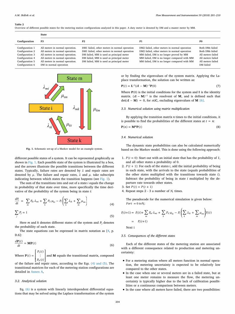
different possible states of a system. It can be represented graphically asshown in Fig. 1. Each possible state of the system is illustrated by a box,and the arrows illustrate the possible transitions between the differentstates. Typically, failure rates are denoted by λ and repair rates aredenoted by μ. The failure and repair rates, λ and μ, take subscriptsindicating between which states the transition happens (see Fig. 1).

The sum of the transitions into and out of a state i equals the changein probability of that state over time, more specifically the time deri-vative of the probability of the system being in state i:

∑ ∑ ∑ ∑= + − ⎛

⎝⎜ + ⎞

⎠⎟

dPdt

P λ P μ P λ μ· · ·i

mm mi

kk ki i

kik

mim

(4)

∑ =P 1j

j(5)

Here m and k denotes different states of the system and Pj denotesthe probability of each state.

The state equations can be expressed in matrix notation as [4, p.D.6]:

=d tdt

tP MP( ) ( )(6)

Where =⎡

⎣

⎢⎢

⋮⎤

⎦

⎥⎥

tP t

P tP( )

( )

( )N

1and M equals the transitional matrix, composed

of the failure and repair rates, according to the Eqs. (4) and (5). Thetransitional matrices for each of the metering station configurations aredetailed in Annex A,

3.2. Analytical solution

Eq. (6) is a system with linearly interdependent differential equa-tions that may be solved using the Laplace transformation of the system

or by finding the eigenvalues of the system matrix. Applying the La-place transformation, the solution can be written as:

= −− −t sP L I M P( ) ( ) (0)1 1 (7)

Where P(0) is the initial conditions for the system and I is the identitymatrix. − −sI M( ) 1 is the resolvent of M, and is defined such thatdet −sI M( ) = 0, for ∈s C, excluding eigenvalues of M [6].

3.3. Numerical solution using matrix multiplication

By applying the transition matrix n times to the initial conditions, itis possible to find the probabilities of the different states at t = n:

=n tP M P( ) ( )n (8)

3.4. Numerical solution

The dynamic state probabilities can also be calculated numericallybased on the Markov model. This is done using the following approach:

1. =P t( 0): Start out with an initial state that has the probability of 1,and all other states a probability of 0.

2. +P t( 1): For each of the states i, add the initial probability of beingin each state, with the arrivals to the state (equals probabilities ofthe other states multiplied with the transitions towards state i).Subtract the probability of being in state i multiplied by the de-parture rate towards other states.

3. Set = +P t P t( ) ( 1)4. Repeat steps 2 - 3 a number of Nt times.

The pseudocode for the numerical simulation is given below:=Fort toN0 :t

∑ ∑ ∑ ∑+ = + + − ⎛

⎝⎜ + ⎞

⎠⎟

= +

P t P t P λ P μ P λ μ P t

P t

( 1) ( ) · · · ( )

( 1)

i im

m mik

k ki ik

ikm

im i

i

Next i

3.5. Consequences of the different states

Each of the different states of the metering station are associatedwith a different consequence related to production and metering un-certainty:

• For a metering station where all meters function in normal opera-tion, the metering uncertainty is expected to be relatively lowcompared to the other states.

• In the case when one or several meters are in a failed state, but atleast one meter remains to measure the flow, the metering un-certainty is typically higher due to the lack of calibration possibi-lities or a continuous comparison between meters.

• In the case where all meters have failed, there are two possibilities:

Table 2Overview of different possible states for the metering station configurations analyzed in this paper. A duty meter is denoted by DM and a master meter by MM.

State

Configuration P3 P2 P1 P0

Configuration 1 All meters in normal operation. DM1 failed, other meters in normal operation DM2 failed, other meters in normal operation Both DMs failedConfiguration 2 All meters in normal operation. DM1 failed, other meters in normal operation DM2 failed, other meters in normal operation Both DMs failedConfiguration 3 All meters in normal operation. DM failed, MM is used as principal meter MM failed, DM is no longer proved by MM All meters failedConfiguration 4 All meters in normal operation. DM failed, MM is used as principal meter MM failed, DM is no longer compared with MM All meters failedConfiguration 5 All meters in normal operation. DM failed, MM is used as principal meter MM failed, DM is no longer compared with MM All meters failedConfiguration 6 DM in normal operation DM failed

Fig. 1. Schematic set-up of a Markov model for an example system.

A.M. Skålvik et al. Flow Measurement and Instrumentation 59 (2018) 201–210

204

- Continue production without measurement until the nextplanned production stop. This results in a high uncertainty due tothe lack of dedicated measurement.- Shut down production during the time it takes to repair themeter(s).

In [7], Stockton shows a methodology to express the potential loss Qfrom absolute expanded measurement uncertaintyU with the followingrelation:

= = ≈Q potential loss Uπ

U8

0.2·(9)

Here U is the absolute expanded uncertainty (95% confidence level)of the value of the quantity that is measured by the metering station.The π1/ 8 factor comes from integrating the assumed normal dis-tribution curve of the measurement from -∞ to 0 (thoroughly explainedin [7]).

Using the previously introduced subscript i to designate a specificstate i of the system and introducing the time dependence, as well asexpressing the absolute uncertainty in terms of relative uncertaintymultiplied by production value, Eq. (9) can be rewritten as:

=Q t U V t( ) 0.2· *· ( )i i (10)

Here the production value V t( ) is the discounted value of the pro-duction that is measured by the metering station at time t, andU*i is therelative expanded uncertainty (95% confidence level) associated withthe metering station in state i.

In the case where all meters have failed and the production is shutdown, the expected loss may be estimated to be the value of the delayedproduction.1

=Q t V t( ) ( )shutdown (11)

Note that this may be a simplification, and that an investigation ofdifferent ways to quantify the consequence of a shut down is outside thescope of this paper.

4. Input data

In this section we will establish the example input data that will beused to perform an example risk-cost-benefit analysis. Note that theinput data depends on the different systems and different meteringstations, and are only example values.

Uncertainties associated with different states: The uncertaintiesof the different meters are example values only, and the example valuesin this paper are set based on the calibration and control possibilitiesand engineering judgement. For a duty meter proved with a proverdevice in a bypass loop, the uncertainty is assumed to be 0.25% U*(relative expanded uncertainty with 95% confidence level). This is the

case for the two duty meters in parallel in configuration 1 in Table 1.When the duty meter is proved with a master meter installed in a

bypass loop, which is the case for configuration 2 and 3 in Table 1, theuncertainty is assumed to be slightly higher, in this example 0.30% U*.If one of the meters in configuration 3 are in a failed state, the re-maining meter will still have the possibility of calibration through theCP. Due to lack of opportunity for comparison between DM and MM, itis assumed that the remaining meter will have an uncertainty of 0.50%U*.

In configuration 4 in Table 1, where the duty meter is in-line withthe master meter, the duty meter uncertainty is assumed to be 0.40%U* and in the case where only one meter is in function, the uncertaintyis assumed to be 1.0% U*. In configuration 5 there is no longer a ca-libration possibility with a compact prover, and the uncertainty is as-sumed to be 0.60% U* for the case where both meters function and1.50% U* if one of the meters are in a failed state.

In configuration 6 in Table 1, where there is only one meter left inthe metering station, without proving or calibration, the metering un-certainty is assumed to be 1.50% U*.

Table 3 gives an overview of the different uncertainties associatedwith the different states of the meter station configurations.

Mean Time Between Failures (MTBF) and Mean Time To Repair(MTTR): The transition rates between the different states can be cal-culated using the following expressions:

= =λMTBF

μMTTR

1 , 1

Here λ is the failure rate, μ is the repair rate. MTBF is the expectedtime before a new or repaired meter fails and can no longer be used toadequately measure the produced flow. MTTR is the expected time ittakes before a meter in a failed state is repaired or replaced.

For a meter in-line with the flow, the mean time between failuresmay be set to 4 years of operation as an example:

= = −λMTBF

days1 11460inline

inline

1

Due to less wear and tear from the flow, the mean time betweenfailures of a meter in a bypass loop is as an example value set to beapproximately four times higher.

= = −λMTBF

days1 15480bypass

bypass

1

As an example, it is assumed that a meter which is placed in a by-pass loop may be repaired or replaced within 2 days:

= = −μMTTR

days1 12direct

direct

1

For a meter that is in-line with the flow it is assumed that it cannotbe repaired or replaced before a production stop. If a planned pro-duction stop occurs for example every 5 years, in the cases where it ispossible to wait for a planned production stop, the mean time to repairis assumed to be in the order of 2.5 years:

= = −μMTTR

days1 12.5·365wait

wait

1

It is important that the simulation step size is chosen so that there isonly incremental change in the state probabilities between each step.

Production profile: Fig. 2 illustrates the example production pro-file that is used in the calculations in this paper. Note that for simplicity,the effect on the production of the planned production stops is nottaken into account here.

Oil price: An illustrative oil price of 50 USD/barrel is used as anexample.

Net present value: The net present value is estimated according toEq. (2). Note that in this paper, the discount rate, r, is set to 0 forsimplicity, as this will be a company-specific parameter.

Table 3Overview of uncertainties associated with the different states of the metering stationconfigurations.

Metering station State 3 (all metersfunction)

State 1 or 2 (one meterfailed)

Configuration 1 0.25 0.25Configuration 2 0.30 0.30Configuration 3 0.30 0.50Configuration 4 0.40 1.00Configuration 5 0.60 1.50Configuration 6 1.50 –

1 This is the case that will be studied in the example calculation in this paper. Note thatanother possible consequence could be that the production is not shut down, and the uncertaintyof the flow rate then is calculated based upon the available information from i.e. allocationmeasurements upstream of the metering station.

A.M. Skålvik et al. Flow Measurement and Instrumentation 59 (2018) 201–210

205

CAPEX and OPEX of the different metering stations: The CAPEX,or capital expenditure, includes costs related to procurement and in-stallation of the meters, including engineering resources as well as thefootprint of the metering station on the platform. The OPEX, or op-erational expenditure, includes operational costs associated withmaintenance, proving and calibration.

Table 4 shows an example values of CAPEX and OPEX for the dif-ferent configurations Table 1. The costs for configurations 1 and 6 areestimated based on an example in [8]. The other costs have been esti-mated assuming that both CAPEX and OPEX are roughly proportional tothe number of meters.

Note that the costs in Table 4 are only examples values, and are onlyquantified here in order to illustrate the risk-cost-benefit analysis. Thecost may vary significantly between the different installations, anddepends on material costs, cost of engineering hours and maintenance,as well as how the weight and dimension footprint on the platform isvaluated.

5. Results

This section shows results of the risk-cost-benefit analysis based onthe example input parameters introduced in chapter 6. First, we showthe probabilities for the different system states, calculated based uponexample MTBF and MTTR given in chapter 5, using the Markov modeland numerical simulation as described in chapter 5. Then we use theseprobabilities combined with example uncertainties, oil price, CAPEXand OPEX from chapter 6 to perform a risk-cost-benefit analysis foreach of the metering stations.

5.1. System state probabilities

Fig. 3–6 show the various system state probabilities for the differentmetering station configurations, based on the example MTBF and MTTRas introduced in chapter 6.

As shown in Table 2, we define four different system states:For configurations 1 and 2:

P3: Probability of all meters in normal operationP2: Probability that duty meter 1 has failed

Fig. 2. Example daily production profile of the flow that will be measured in the meteringstation.

Table 4Example CAPEX and OPEX for the different metering station configurations.

Metering station CAPEX (year 1) OPEX / year[kUSD] [kUSD]

Configuration 1 5 000 2 000Configuration 2 3 000 1 200Configuration 3 2 250 900Configuration 4 1 800 720Configuration 5 1 000 400Configuration 6 500 200

Fig. 3. Probability for being in different system states for configurations 1 and 2. Notethat the probabilities for P_0, P_1 and P_2 are so small that they are not visible in the plot.

Fig. 4. Probability for being in different states for configuration 3.

Fig. 5. Probability for being in different states for configurations 4 and 5.

Fig. 6. Probability for being in different states for configuration 6.

A.M. Skålvik et al. Flow Measurement and Instrumentation 59 (2018) 201–210

206

P1: Probability that duty meter 2 has failedP0: Probability that both duty meters have failedFor configurations 3, 4, 5 and 6:P3: Probability of all meters in normal operationP2: Probability that the master meter has failedP1: Probability that the duty meter has failedP0: Probability that all meters have failed

Fig. 3 shows that for configuration 1 and 2, the probabilities thatone or two meters have failed are small compared to the probabilitythat all meters are in normal operation. This is due to the fact thatsince the duty meters are installed in parallel, the expected time torepair a failed meter is relatively short since it is possible to repair orreplace the meter directly without waiting for a planned productionstop.

For configuration 3 (Fig. 4), the probability that the duty meter is ina failed state (P )1 is no longer negligible to the probability of all metersin normal operation (P3). The reason why P1 is higher here than forconfigurations 1 and 2 is that in this configuration the duty meter is in-line with the flow and cannot be repaired or replaced during produc-tion, and the flow is therefore measured using the master meter untilthe next planned production stop. P2, the probability that the mastermeter is in a failed state is relatively small, as the master meter is in abypass loop and may be repaired or replaced during production. For thesame reason, the probability that both meters have failed P( )0 is alsorelatively small.

For configurations 4 and 5 (Fig. 5), probabilities that the duty meteror the master meter is in a failed state (P1 and P )2 are no longer negli-gible compared to the probability of all meters in normal operation (P3).This is the result of installing both meters in series, as the meters cannotbe repaired or replaced during production. If both meters are in a failedstate, the production is stopped temporarily and both meters are re-placed. The probability P0 that both meters have failed is thereforerelatively small.

For configuration 6 (Fig. 6), the production is shut down and themeter replaced directly if the only meter fails. The probability that theonly meter is in a failed state is therefore very low.

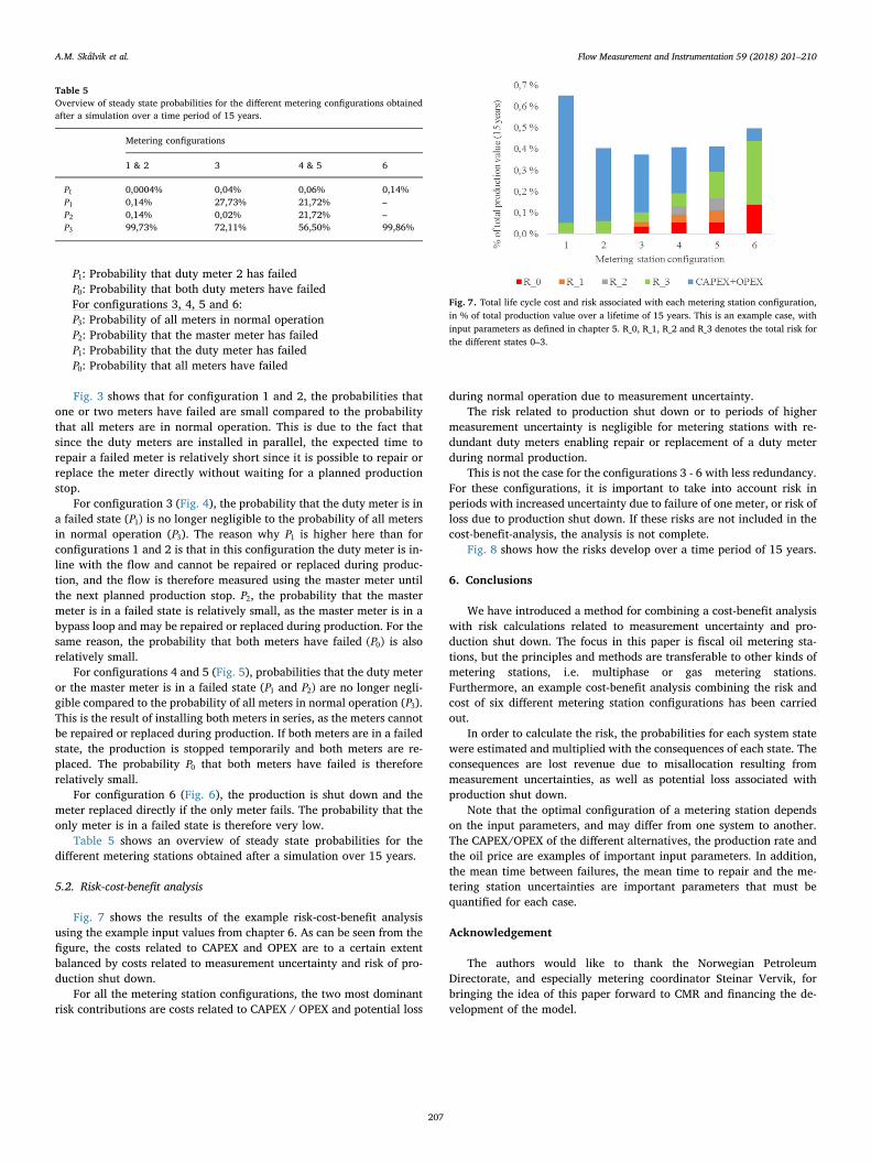
Table 5 shows an overview of steady state probabilities for thedifferent metering stations obtained after a simulation over 15 years.

5.2. Risk-cost-benefit analysis

Fig. 7 shows the results of the example risk-cost-benefit analysisusing the example input values from chapter 6. As can be seen from thefigure, the costs related to CAPEX and OPEX are to a certain extentbalanced by costs related to measurement uncertainty and risk of pro-duction shut down.

For all the metering station configurations, the two most dominantrisk contributions are costs related to CAPEX / OPEX and potential loss

during normal operation due to measurement uncertainty.The risk related to production shut down or to periods of higher

measurement uncertainty is negligible for metering stations with re-dundant duty meters enabling repair or replacement of a duty meterduring normal production.

This is not the case for the configurations 3 - 6 with less redundancy.For these configurations, it is important to take into account risk inperiods with increased uncertainty due to failure of one meter, or risk ofloss due to production shut down. If these risks are not included in thecost-benefit-analysis, the analysis is not complete.

Fig. 8 shows how the risks develop over a time period of 15 years.

6. Conclusions

We have introduced a method for combining a cost-benefit analysiswith risk calculations related to measurement uncertainty and pro-duction shut down. The focus in this paper is fiscal oil metering sta-tions, but the principles and methods are transferable to other kinds ofmetering stations, i.e. multiphase or gas metering stations.Furthermore, an example cost-benefit analysis combining the risk andcost of six different metering station configurations has been carriedout.

In order to calculate the risk, the probabilities for each system statewere estimated and multiplied with the consequences of each state. Theconsequences are lost revenue due to misallocation resulting frommeasurement uncertainties, as well as potential loss associated withproduction shut down.

Note that the optimal configuration of a metering station dependson the input parameters, and may differ from one system to another.The CAPEX/OPEX of the different alternatives, the production rate andthe oil price are examples of important input parameters. In addition,the mean time between failures, the mean time to repair and the me-tering station uncertainties are important parameters that must bequantified for each case.

Acknowledgement

The authors would like to thank the Norwegian PetroleumDirectorate, and especially metering coordinator Steinar Vervik, forbringing the idea of this paper forward to CMR and financing the de-velopment of the model.

Fig. 7. Total life cycle cost and risk associated with each metering station configuration,in % of total production value over a lifetime of 15 years. This is an example case, withinput parameters as defined in chapter 5. R_0, R_1, R_2 and R_3 denotes the total risk forthe different states 0–3.

Table 5Overview of steady state probabilities for the different metering configurations obtainedafter a simulation over a time period of 15 years.

Metering configurations

1 & 2 3 4 & 5 6

P0 0,0004% 0,04% 0,06% 0,14%P1 0,14% 27,73% 21,72% –P2 0,14% 0,02% 21,72% –P3 99,73% 72,11% 56,50% 99,86%

A.M. Skålvik et al. Flow Measurement and Instrumentation 59 (2018) 201–210

207

Annex A. Markov models and transitional matrices for the different metering station configurations

See Fig. 9–12.The method and notation are explained in chapter 4.Metering station configurations 1 and 2:

=

⎡

⎣

⎢⎢⎢⎢

−− −

− −−

⎤

⎦

⎥⎥⎥⎥

μ λ λλ μ λ

λ μ λμ μ μ λ

M

1 00 1 00 0 1

1 2

direct inline inline

inline direct inline

inline direct inline

direct direct direct inline

1 2,

Metering station configuration 3:

=

⎡

⎣

⎢⎢⎢⎢

−− −

− −− −

⎤

⎦

⎥⎥⎥⎥

μ λ λλ μ λ

λ μ λμ μ μ λ λ

M

1 00 1 00 0 1

1

direct inline inline

inline wait inline

inline direct bypass

direct wait direct bypass inline

3

Fig. 8. Risk-cost benefit analysis for different me-tering station configurations. Input parameters asdescribed in chapter 6. R_0, R_1, R_2 and R_3 denotesthe total risk for the different states 0–3. Note thatthe simulations are run for each year, but to improvereadability the plots are continuous.

A.M. Skålvik et al. Flow Measurement and Instrumentation 59 (2018) 201–210

208

Metering station configurations 4 and 5:

=

⎡

⎣

⎢⎢⎢⎢

−− −

− −−

⎤

⎦

⎥⎥⎥⎥

μ λ λλ μ λ

λ μ λμ μ μ λ

M

1 00 1 00 0 1

1 2

direct inline inline

inline wait inline

inline wait inline

direct wait wait inline

4 5,

Fig. 9. Markov model for metering stations 1 and 2.

Fig. 10. Markov model for metering station 3.

Fig. 11. Markov model for metering stations 4 and 5.

Fig. 12. Markov model for metering station 6.

A.M. Skålvik et al. Flow Measurement and Instrumentation 59 (2018) 201–210

209

Metering station configuration 6:

=⎡

⎣

⎢⎢⎢

−

−

⎤

⎦

⎥⎥⎥

μ λ

μ λ

M

1 0 00 0 0 00 0 0 0

0 0 1

direct inline

direct inline

6

References

[1] G.D.F. Philip Chan, E. Suez, P. Norge, AS, Bruk av usikkerhetsanalyser ognåverdiberegninger i konseptfasen, NFOGM nytt nr 2, 2014.

[2] NORSOK, Annex C, System selection criteria (informative), NORSOK, 2014.[3] AstridMarie Skålvik, RanveigNygaard Bjørk, Kjell-Eivind Frøysa, Camilla Sætre, A

new methodology for cost-benefit-risk analysis of oil metering station lay-outs, in:Proceedings of the 33rd North Sea Flow Measurement Workshop, Tønsberg, 2015.

[4] Aven Terje, Pålitelighets og risikoanalyse, Universitetsforlaget, 1994.

[5] ISO/IEC, Uncertainty of measurement - part 3: Guide to the expression of uncertaintyin measurement, ISO/IEC, Geneva, 2008.

[6] G. Strang, Differential Equations and Linear Algebra, Wellesley-Cambridge, 2014.[7] Philip Stockton, Cost benefit analysis in the design of allocation systems, in:

Proceedings of the 27th International North Sea Flow Measurement Workshop,Tønsberg, Norway, 2009.

[8] Dag Flølo, Statoil, Cost benefit analysis for measurement at pipeline entry, NFOGMHydrocarbon Management Workshop – Field Allocation 2014, 2014.

A.M. Skålvik et al. Flow Measurement and Instrumentation 59 (2018) 201–210

210