Master’s Thesis

Flexural Buckling of General Beam Systems

A Method to Determine K-factors using Energy Considerations

Jacob S. Mortensen

Mikael Hansen

2012

i

Preface

This Master’s thesis ”Flexural Buckling of General Beam System – A Method to

Determine K-factors using Energy Considerations” is made by Jacob S. Mortensen and

Mikael Hansen during the 4th semester of the Master’s Degree of Structural and Civil

Engineering at Aalborg University Esbjerg. The project was completed within the period

of 1st of February and 14th of June 2012.

We want to thank Lars Damkilde for his assistance and supervision during the semester.

Furthermore we want to thanks ISC A/S for the exchange of expertise and knowledge and

for providing office space and supplies.

There will regularly be referred to appendices, these are placed in continuation of the

report. Annexes containing material used to produce the report and appendices are placed

on the enclosed CD-ROM.

Appendices:

Appendix 1: Examples of Methodical and Experience Based Approaches

Appendix 2: Verification of Cross-section input in Strain Energy Calculations

Appendix 3: Critic of Iterative System Buckling Approach

Appendix 4: Journal Paper (DRAFT)

Annexes:

Annex 1: Structural Drawings

Annex 2: MATLAB script

Enclosed:

One CD-ROM with original documentation for the project:

Master’s Thesis incl. appendices

Annexes

Abstract

When designing according to the Eurocode, structures, that are not especially sensitive to

non-linear behavior, are comprised by an individual member check. This member check

includes a reduction factor to account for imperfections. The reduction factor is primarily

dependent on the critical load, and this is why the determination of K-factors for

individual member becomes important. Traditionally the individual K-factors are

determined by methodical approaches such as the isolated subassembly or story methods.

These methods do not take the actual system behavior into account, as the linear buckling

analysis does. The system buckling approach, which uses the linear buckling analysis, is

preferable when the structural behavior is complex, however the method contains the

paradox, that compressive members with an relatively small axial force yields excessively

large K-factors. In the present thesis a method to circumvent this paradox is proposed.

The method distinguishes between members being prone to buckling and members that

are not sensitive to additional axial load. Based on energy considerations the load

multiplier found by the linear buckling analysis is weighed for each member. The

proposed method is verified by 2D examples, where comparisons to known methods are

made. It is found that the proposed method provides reasonable K-factors, and it is

believed, that future work on the method could lead to an implementation in software,

which provides automated code check. Thereby the burdensome manually definition of

critical length for each members is avoided.

ii

Contents:

1. Introduction .......................................................................................................................... 1

1.1 Motivation .............................................................................................................................. 1 1.2 Stability Considerations in Design ......................................................................................... 3 1.3 Current Approaches for Determining the K-Factor ............................................................... 4 1.4 Project Objective .................................................................................................................... 4

2. Stability of Columns – Calculation of Perfect and Real Columns ................................... 6

2.1 Derivation of the K-factor using the Differential Equation for a Beam Element .................. 6 2.2 Calculation of Columns According to EN 1993 – Including Imperfections .......................... 8 2.2.1 Column with an imperfection – Ayrton-Perrys formula .................................................. 9 2.2.2 Column formula in EN 1993 ......................................................................................... 10 2.3 Summary .............................................................................................................................. 13

3. Methodical Approach to Stability of Beam-column Systems ......................................... 14

3.1 Categorization into sway and non-sway systems ................................................................. 14 3.2 Stability of Frame Systems Based on the Isolated Subassembly Approach ........................ 16 3.3 Stability of Frame Systems Based on the Story Method Approach ..................................... 19 3.4 Summary .............................................................................................................................. 20

4. Numerical approach to Stability of Beam-column Systems ........................................... 21

4.1 The Linear Eigenvalue Problem – Load Multiplication Factor ........................................... 21 4.1.1 Member division ............................................................................................................ 23 4.1.2 Results When Using Shear-Flexible Beam Elements .................................................... 24 4.2 System Buckling Approach .................................................................................................. 25 4.3 The Paradox Concerning Large K-factors ........................................................................... 26 4.3.1 L-frame – K-factor Dependence to Load Case .............................................................. 26 4.3.2 Verification of the K-factor Paradox ............................................................................. 30 4.4 Iterative System Buckling Approach ................................................................................... 33 4.5 Summary .............................................................................................................................. 34

5. Proposed Method – The Energy Ratio Method ............................................................... 35

5.1 Energy Based Stability Considerations of a Beam Member ................................................ 35 5.1.1 Analytical calculation of energy .................................................................................... 35 5.1.2 Numerical calculation of energy .................................................................................... 36 5.1.3 Verification of Energy Calculation ................................................................................ 37 5.2 The Proposed Method .......................................................................................................... 40 5.3 Demonstration of the Energy Ratio Method ........................................................................ 41 5.3.1 Simply Supported L-frame ............................................................................................ 41 5.4 Other Application of the Energy Ratio Method ................................................................... 44 5.5 Summary .............................................................................................................................. 46

6. Comparison of Proposed Method to Other Known Methods ........................................ 48

6.1 Model Description ................................................................................................................ 48 6.2 Results Compared to the Energy Ratio Method ................................................................... 48 6.2.1 Similar Results Found by the ERM Compared to Other Known Methods.................... 49 6.2.2 Inconsistent Results Found by the ERM Compared to Other Known Methods ............ 50 6.3 Summary .............................................................................................................................. 51

7. Conclusion ........................................................................................................................... 52

References ........................................................................................................................................ 53

iii

Figures:

Figure 1-1 Failure in slender chord at Cowboys Stadium, Dallas, USA ............................................ 1 Figure 1-2 Failure in slender chord at Cowboys Stadium, Dallas, USA ............................................ 2 Figure 1-3 Experiments to determine non-linear behavior of columns .............................................. 2 Figure 1-4 Flowchart of the design procedure according to Eurocode .............................................. 3 Figure 2-1 Basis for differential equation for a beam column ........................................................... 6 Figure 2-2 Critical lengths for basic cases ......................................................................................... 8 Figure 2-3 Flexible end restraints....................................................................................................... 8 Figure 2-4 Imperfect column ............................................................................................................. 9 Figure 2-5 Design equations for members subjected to axial load and bending .............................. 12 Figure 2-6 Buckling curve dependence of cross section .................................................................. 12 Figure 2-7 Imperfection factor dependence of buckling curve ........................................................ 13 Figure 2-8 Buckling curves .............................................................................................................. 13 Figure 3-1 Boundary conditions for a sway frame ........................................................................... 14 Figure 3-2 Boundary conditions for a non-sway frame ................................................................... 14 Figure 3-3 First mode shape for sway frame .................................................................................... 15 Figure 3-4 First modeshape for non-sway frame ............................................................................. 15 Figure 3-5 Stiffness designations for surrounding columns ............................................................. 17 Figure 3-6 Critical length ratio for a column in a non- sway mode ........................................... 18 Figure 3-7 Critical length ratio for a column in sway mode ...................................................... 18 Figure 4-1 Flowchart of numerical process ...................................................................................... 21 Figure 4-2 Buckling modeshape of simply supported column ......................................................... 23 Figure 4-3: Buckling modeshape of a column with fixed support at the ends. ................................ 24 Figure 4-4 Deviation of results using shear-flexible beam elements compared to classic analytical

theory ....................................................................................................................................... 25 Figure 4-5 Model used for illustrating the influence of tension/compression in a member adjacent

to a column .............................................................................................................................. 27 Figure 4-6 K-factor at various axial force in adjacent horizontal member ...................................... 27 Figure 4-7 Reduction factor according to EN-1993 at various axial force in adjacent horizontal

member .................................................................................................................................... 28 Figure 4-8 Mode shape when tension in horizontal member is very large ...................................... 29 Figure 4-9 Mode shape when compressive axial force is equal in both members ........................... 29 Figure 4-10 Calculated K-factors ..................................................................................................... 30 Figure 4-11 Calculated reduction factor according to EN-1993 ...................................................... 30 Figure 4-12 Model consisting of two members with small and large axial force respectively ........ 31 Figure 4-13 First mode ..................................................................................................................... 31 Figure 4-14 Additional load applied at the top of the vertical column ............................................ 32 Figure 5-1 The difference between the system buckling approach and the proposed method ......... 35 Figure 5-2 Column considered for energy calculation ..................................................................... 36 Figure 5-3 Model used for energy demonstration ............................................................................ 38 Figure 5-4 Energy calculated numerical by MATLAB script .......................................................... 39 Figure 5-5 Energy calculated with twice the number of elements ................................................... 39 Figure 5-6 Model produced by MATLAB script providing K-factors by both ERM and SBA ...... 42 Figure 5-7 K-factors for Member1 found by ERM and SBA .......................................................... 42 Figure 5-8 Plot of K-factors for Member1 in reduced interval of load cases ................................... 43 Figure 5-9 Model showing buckling at the same time for both members ........................................ 43 Figure 5-10 K-factors for Member2 found by ERM and SBA ........................................................ 44 Figure 5-11 Model used to illustrate iterative procedure to find same time buckling...................... 45 Figure 5-12 First iterative step: Energy ratios approaches one ........................................................ 45 Figure 5-13 Second iterative step: Energy ratios have become one for both members ................... 46 Figure 6-1 Model of the three story building ................................................................................... 48 Figure 6-2 Results graphically displayed ......................................................................................... 49 Figure 6-3 Modeshape of three story building where axial load increases down the columns ........ 50 Figure 6-4 Example from Choi and Yoo (2008) .............................................................................. 51

iv

Tables:

Table 4-1 Buckling analysis for simply supported column .............................................................. 23 Table 4-2: Buckling analysis for a column with fixed support at the ends ...................................... 24 Table 4-3 Sectional forces, reduction factors and utilization ratios ................................................. 32 Table 4-4 Sectional forces, reduction factors and utilization ratios after increasing the critical load

in the vertical member ............................................................................................................. 33 Table 5-1 Comparison between analytically and ERM based energy calculations .......................... 40 Table 5-2 K-factors found by traditional SBA, improved SBA and ERM ...................................... 46 Table 6-1 Sectional properties ......................................................................................................... 48 Table 6-2 Comparison of K-factors ................................................................................................. 49

1

1. Introduction

Almost all structures consist of compression members which mean a risk of instability. In the

European standards, a stability check often comprise of a check of the individual members.

When doing so, a critical length of the compression member is needed as it defines the elastic

critical load. The critical length can be determined in a number of ways, either by desk

calculation or computer based methods. Most desk calculation approaches are based on a

number of assumptions in order to match an analytical solution, therefor the usability of these

methods are limited. It also means that these methods are made for specific cases, which for

the most part means regular frames. When violating these assumptions, the error can be hard

to estimate.

When evaluating structures that cannot be classified as a regular frame by a number of stories

and/or bays, the critical length are either determined by experience and standard values or by

computer based calculations such as a system buckling approach. The system buckling

approach is not limited to specific cases and therefor offers a wide usability. This method does

however contain a paradox which means that compression members with a small axial force

yields excessively long critical lengths. Therefore a method is needed that overcomes this

paradox [1][14].

1.1 Motivation

The stability of structures is becoming harder to evaluate as the complexity of structures

increases. The common practice today often relies on methodical approaches and experience

to interpret results, where wrongly estimated critical length can lead to disastrous results. In

the following pictures, the collapsed practice facility at Dallas Cowboys Stadium is seen. The

failure was progressed from buckling in the inner chord of the frame.

Figure 1-1 Failure in slender chord at Cowboys Stadium, Dallas, USA

2

Figure 1-2 Failure in slender chord at Cowboys Stadium, Dallas, USA

In the design aspect instability is a non-linear phenomenon, which in most cases can be

handled with linear analysis according to standards as the Eurocode (see section 1.2). The

structural integrity is secured by reducing the sectional axial capacity by a factor, which

account for the non-linear behavior. This factor have been determined by various experiment

of columns with various slenderness and adapted in standards such as the Eurocode.

Figure 1-3 Experiments to determine non-linear behavior of columns

In new designs the critical lengths are usually estimated conservatively (at least when the

engineer does not overlook a sway system behavior), and the need for accurate estimates of

critical lengths are not that important. However, when performing re-analysis of structures due

to changed requirements of the structure, the accuracy of the calculation may become crucial.

In Europe the common practice is to design for stability using the Eurocode. Current software

that offers a code-check based on the Eurocode requires the critical length to be set manually.

A programmable and reliable method of determining the K-factor, which can be added to the

code-check programs, would ease the stability calculations.

3

1.2 Stability Considerations in Design

The Eurocode defines how the stability analysis should be performed based on the current

load level. The load multiplier is found using a linear buckling analysis and it determines how

the stability check should be performed.

If the load multiplier is above 10 and 2nd order effects can be neglected, then the stability can

be calculated by checking the individual elements. This requires the determination of the

critical load or critical length which are interdependent (In the engineering terminology the

critical length is normally defined relative to its physical length by the K-factor).

If the load multiplier is below 10 and 2nd order effects should be taking into account, then the

method used to check for stability can be chosen according to the sensitivity to 2nd order

effects.

The decision procedure is summarized in the flow chart below [6].

Figure 1-4 Flowchart of the design procedure according to Eurocode

Estimating an appropriate K-factor for individual elements in a system composed of several

elements becomes important in three out of four methods given in the flow chart (marked with

red).

4

1.3 Current Approaches for Determining the K-Factor

Besides guessing the K-factors based on experience, there are three main different approaches

to calculate the K-factor: The isolated subassembly approach, the story method approach and

the system buckling approach.

The isolated subassembly approach is methodical approach which is widely used to determine

the K-factor of a single column. This is done by assessing the ratio of stiffness between the

column and the adjacent columns and beams. This approach has limiting assumptions. Gantes

and Mageirou (2005) has proposed an improved method for calculation the K-factor for a

single column in a multi-story sway frame which account for all rotation and translation

boundary conditions at the beam ends [1][5][12].

The story method approach is a methodical approach, which is used for regular steel frames

and assumes that the shear force can be transferred between columns in a story. This means

that the weaker columns are supported against sidesway by the stronger ones. The sidesway

buckling resistance is assumed to be equal to the total sidesway resistance of all the columns

in that story, which yields a unified K-factor for all members in a story. Two versions of the

story method are used and they differ in the way the total resistance is calculated. One

method, the story buckling method, uses the isolated subassembly method to determine the

critical load for an entire story. The other method, the story stiffness method, uses the first

order lateral displacements to include interaction between stories [1].

The system buckling approach uses a linear buckling analysis to determine a load multiplier

for the system and thereby a critical load for the entire system. The critical load of each

member is calculated by multiplying the axial force in the member with the system load

multiplier. When the critical load is calculated a K-factor can be derived. This method’s

strong point is that it accounts for the entire system behavior, but it also presents the paradox

that a small axial compression forces will yield small critical load, and thereby a large K-

factor [1].

This paradox is mentioned in other papers and an iterative method has been proposed in order

to overcome this problem. The main idea behind the method is that an increase in axial force

in some members only has a small effect on the load multiplier. By adding fictitious axial

force a higher critical load and thereby a smaller K-factor can be obtained. An iterative

procedure has been proposed, where the axial force is increased while calculating the change

in K-factor after each step. This is done until the change in K-factor is sufficiently small in all

members [1][7][9].

1.4 Project Objective

The main objective of this project is to propose a new method that overcomes the weakness of

the system buckling approach when calculating the critical load or critical length for

individual members in a system. The method should be programmable in traditional FE-code,

and thereby easily implemented into existing software with code-check capabilities. The goal

is a method that does not require any user input, besides what is usually given.

In the first part of the project (Chapter 2), the concept of stability of a single member is

outlined. Both perfect and imperfect columns are considered, and the design criteria according

to the Eurocode are defined.

In the middle part of the project (Chapter 3 and 4), the theory behind the most commonly used

methods is presented. Both methodical and numerical method applies for a system of

members, however each method has its limitations or disadvantages.

The last part of the project (Chapter 5 and 6) contains the proposition of a new method,

referred to as the Energy Ratio Method, for calculating the K-factors. Demonstrative examples

showing results of the Energy Ratio Method on simple 2D cases are used to verify the

method. Furthermore the method is compared with the other known methods described in

Section 1.3.

5

Scope of this project

The Eurocode EN1993 (EC3) is used in many countries today and this project will

only focus on design according to this code.

Only steel structures will be considered

All joints between members are assumed to be rigid.

Cross sections are assumed to be uniform.

Only elastic buckling is considered, i.e. no plastic hinges.

The proposed method is only verified using 2D systems.

6

2. Stability of Columns – Calculation of Perfect and Real Columns

In this chapter, the stability of a column as a single member using an analytical approach is

described.

Firstly, the concept of a columns critical length (also called effective length, free length,

reduced length or buckling length) is outlined by considering a perfect column, i.e. no

imperfection is considered.

Secondly, the fact that perfect columns do not occur in real structures, means that

imperfections have to be taken into account. The design of structures is governed by design

codes, and the approach for including imperfections according to design code EN 1993 is

explained.

2.1 Derivation of the K-factor using the Differential Equation for a Beam Element

Using the differential equation for bending in a beam-column it is possible to derive the

critical axial load for an ideal column, as done by Timoshenko [14].

Figure 2-1 Basis for differential equation for a beam column

Based on the beam in Figure 2-1 the basic differential equation for a lateral loaded beam

column can be written as:

(1).

As no lateral loads are present when determining the critical load, and by substituting

the equation can be written as:

(2).

The general solution for this equation is:

(3).

The four integration constants are determined by the geometrical and static end restraints of

the beam. These restraints are summarized below:

Fixed end:

Hinge:

Free end:

7

For a column with hinged ends the moments and deflection at the ends of the column are zero

meaning that:

When applying these conditions to the general solution (3) the following is obtained:

As also must equal zero and would give a trivial solution, meaning no

deflection, it is seen that . Therefore:

where gives the lowest critical load.

By inserting and the critical load is found:

√

In this case the critical column length is 1.0 times the actual column length. This is also called

the -factor.

If we look at a column with one end fixed and the other end hinged, also called a propped-end

column, then the restraints become:

By inserting these restraints into the general solution the four restraints becomes:

By combining these four equations it can be shown that

The smallest root to this equation is which gives the follow critical load:

√

Hence a propped-end column has a critical length of times the actual column length.

Based on the preceding examples it is clear that the critical load generally can be written in

the form also known as the Euler load:

(4).

where is the critical column length. Hereby the K-factor for a column is defined,

and it is noted that the critical load and the K-factor are interdependent. If the critical load is

known the K-factor can be determined as:

√

(5).

8

The covered examples and other basic cases can be seen on Figure 2-2.

Figure 2-2 Critical lengths for basic cases

This covers the well-defined end restraints. In the case of flexible end restraints which give an

infinity number of solutions, no general solution can be obtained before the flexibility is

defined. An example is a column whose ends cannot not move but are restrained against

rotation by springs such as seen on Figure 2-3a.

Figure 2-3 Flexible end restraints

Infinity large spring stiffness at both ends will give the same result as a column with fixed

ends, meaning a critical length of . The other limit state is an infinity small spring

stiffness at both ends which corresponds to hinges at both ends and a K-factor of . Hence the

K-factor for such end restraints is in the interval .

The most general case, illustrated in Figure 2-3b, is obtained by applying a rotation spring

(C1) and no movement at one end, and a rotation spring (C2) plus a spring against movement

(C3) at the other end. Such a column has a K-factor in the interval . The infinity

occurs when bottom springs (C2 and C3) are equal to zero, meaning that the column acts as a

cantilever. This combined with a non-existing resistance against rotation in the last spring

(C1) means that the column becomes a mechanism [2].

The critical length or K-factor is a concept derived from perfect columns. Nevertheless the K-

factor is often used as a key parameter in calculations of the strength of compressive elements

in real structures.

2.2 Calculation of Columns According to EN 1993 – Including Imperfections

In real structures, a column will fail before the theoretical critical load is reached. This is due

to various imperfections such as:

Geometrical imperfections: column out-of-straightness, profile tolerances etc.

9

Material imperfections: residual stresses from production or non-linear material be-

havior.

The geometrical imperfections causes amplification to the transverse deflection of the column

which is most pronounced for slender columns.

Non-linear material behavior in steel is experienced when the stress level is larger than

approximately 80 % of the yield stress, also known as the proportional limit. After this point

the modulus of elasticity is reduced and the transverse deflection increases more rapidly. This

effect is not experienced in slender columns were the critical load is reached at a lower stress

level.

Residual stresses become important when the sum of the residual stress and applied stress

exceeds the proportional limit. This can be seen in a welded I-section that buckles about the

minor-axis because there are residual compressive stresses at the free ends of the flanges.

In EN 1993 imperfections are accounted for by introducing a generalized imperfection factor

that covers both geometrical and material imperfections. Ayrton-Perrys formula is an

analytical way of including imperfections and forms the basis for the method used in EN

1993, which is explained in the next sections.

2.2.1 Column with an imperfection – Ayrton-Perrys formula

Ayrton-Perrys formula is the basis for the column strength given in EN 1993 [3]. We consider

a simply supported beam with an imperfection, which is assumed to be a sinus shaped initial

deflection . The model of the imperfect column is seen in Figure 2-4.

Figure 2-4 Imperfect column

If the maximum deflection is , then can be written as:

(

)

(6).

The beam is subjected to an axial force , therefor the bending moment in the beam is:

(7).

where is the total deflection.

10

By inserting in the differential equation for the beam deflection we get:

(8).

where is the modulus of elasticity and is the second moment of inertia.

The differential equation can be solved using the particular solution (

) and the

result is:

(9).

The limit is found when the stress at the edge reaches the yield stress . Using Naviers

formula we get:

(10).

where and is the section area and section modulus respectively. The maximal normal

stress is given by:

(11).

and combining formula (9), (10) and (11) we get:

(12).

The critical stress (Euler stress) is defined as:

(13).

and formula (12) can be written as the Ayrton-Perry formula:

( ) (14).

where

represent the column straightness.

The link between the Ayrton-Perry formula and the column design formula in EN 1993

follows in the next section.

2.2.2 Column formula in EN 1993

In the Ayrton-Perry formula the maximum normal stress is given implicitly. For

convenience the formula is rewritten introducing the column strength reduction factor:

(15).

11

and the non-dimensional slenderness:

√

(16).

By dividing formula (14) with

we get:

( ) (17).

or

( ) (18).

The smallest value of the roots in this quadratic equation is the relevant value of given by:

(( )

)

(19).

Letting the column straightness cover both geometrical and material imperfection by the

expression:

( ) (20).

and introducing:

( ( ) )

(21).

formula (19) can be written as

√

(22).

The last two equations are identical to the ones used in EN 1993-1-1 when calculating

columns, where and the imperfection factor depends on the cross section type,

dimensions and yield stress. The imperfection factor and dependence of cross section can be

seen in Figure 2-6 and Figure 2-7. The reduction factor can be seen in Figure 2-8. The

figures are taken from EN 1991.

The reduction factor is used in the utilization ratio given by:

(23).

where is the cross sectional area, is the yield stress and is the exposed load.

When members are imposed to both axial and bending stress, the axial utilization ratio is

included as part of the total utilization ratio. The utilization ratio in equation (23) is thereby

the first of three terms in the design equations for members subjected to both bending and

12

compression which is seen in Figure 2-5. The two equations express bending about y- and z-

axis respectively.

Figure 2-5 Design equations for members subjected to axial load and bending

Figure 2-6 Buckling curve dependence of cross section

13

Figure 2-7 Imperfection factor dependence of buckling curve

Figure 2-8 Buckling curves

In Figure 2-8 the reduction factor is depends on the non-dimensional slenderness , in

which the K-factor is included by:

√

√

(24).

2.3 Summary

To summarize we now know that the reduction factor is a function the critical load, so even if

the critical value is not reached in real structures, it is still important in the calculations of the

individual member design. Hence, the more precise you can determine the critical length of a

column, the more economical your design can be.

If it is possible to establish the critical load of a column, back calculations can be used to

determine the K-factor by:

√

(25).

The K-factor is determinative for the reduction factor and thereby an important parameter

when calculating the utilization ratio of a compression member by:

(26).

14

3. Methodical Approach to Stability of Beam-column Systems

It is seldom seen that a column acts as an independent column. Often columns are a part of a

larger system of beams which means that the end restraints are flexible. Therefore columns in

such systems are not well-defined as the basic cases, however the basic cases may give the

engineer an idea of in which interval the K-factor is expected to be. The connections between

the beams are often assumed to be rigid, which for the most part is an adequate assumption,

wherefore joint flexibility is not included in the scope of this thesis.

A widely used method for calculating K-factors is the isolated subassembly approach (also

known as the nomograph/alignment chart method), which is presented in pr-EN 1993 amongst

many others. The method requires a categorization of the system into either sway or non-

sway, which is illustrated in Section 3.1. The method is an analytical approach which gives a

correct critical length if several assumptions are fulfilled as explained in Section 3.2.

Due to the fact that these assumptions seldom are fulfilled, other methods have been

developed for typical structures such as rectangular frames or story frames. These methods are

known as story methods and stability calculations concerning both single frames and multi-

bay/multi-story frames are well documented in acknowledged literature [1]. In asymmetric

cases, the story buckling method tends to give better estimates of the K-factors than the

isolated subassembly approach; however in some cases there is significant buckling

interaction between stories, which means that a numerical approach such as the system

buckling approach (see Chapter 4) would be more appropriate. A discussion of these different

approached can be found in (ASCE, 1997) [1]. The two most common story methods are The

Story Buckling Method and The Story Stiffness Method which is outlined in Section 3.3.

3.1 Categorization into sway and non-sway systems

Systems are divided into two different categories: Sway or Non-sway. A sway frame is

allowed to sway to either side, whereas a non-sway frame is restricted from doing so. This is

illustrated on the following figures.

Figure 3-1 Boundary conditions for a sway frame

Figure 3-2 Boundary conditions for a non-sway frame

15

If a linear buckling analysis of the frames is performed, the distorted configurations, also

called mode shapes, are established.

Figure 3-3 First mode shape for sway frame

Figure 3-4 First modeshape for non-sway frame

By comparing the load multiplier (FREQ) in the distorted configurations on Figure 3-3 and

Figure 3-4, it is seen that the general behavior of the system has a large effect on the critical

length of the individual columns. As the load case for the two frames are exactly the same it is

possible to compare the load multiplier directly in order to determining the buckling resistance

of the two systems. The sway frame has a load multiplier of 240 and the non-sway frame a

load multiplier of 2212. This means that the resistance against buckling for the non-sway

frame is about 9 times larger in the given case.

If a standard critical length with the value of the actual member length is assigned for every

member, the risk of overlooking a general system behavior as the one seen on Figure 3-3

arises. Overlooking this means that an individual member check will show a higher buckling

resistance than the system as a whole.

16

3.2 Stability of Frame Systems Based on the Isolated Subassembly Approach

This section contains a description of stability of frames based on annex E of the pr-EN1993

(pre-standard to EC3). The annex provides a mean of establishing the critical length of a

column based on the stiffness of the adjacent beams and the general behavior of the system

(sway or non-sway).

This method is widely used and adopted by both the European and American standards, even

though they are based on different but similar work by Wood (1974) and Julian and Lawrence

(1959) respectively [13][15]. When used on a reference frame with pinned ends base they

provide similar results.

The method described in the European standards offer a higher degree of customization than

the American to overcome violation of some of the assumptions.

The method is based on the following assumptions [1][4][5].

1. All members have constant cross section.

2. All joints are rigid.

3. Behavior is purely elastic.

4. No significant axial compression force exists in the girders.

5. The column stiffness parameter √

must be identical for all columns.

6. Rotations at the far ends of the restraining members are fixed.

7. Joint restraint is distributed to the column above and below the joint in

proportion to of the two columns.

8. The frame is subjected to vertical loads applied only at the joints.

9. All columns in the frame become unstable simultaneously, and no shear force

is transferred to the subassembly from other portions of the structure.

By determining stiffness distribution factors for the end joints of the column in question, a K-

factor is obtained either by using Figure 3-6 (non-sway) and Figure 3-7 (sway), or by using

the conservatively fitted formulas (29) and (30) based on these figures.

By using the following formulas, the distribution factors and are obtained:

(27).

(28).

where

is the column stiffness coefficient

are the stiffness coefficients for the adjacent columns

are the effective beam stiffness coefficients

The stiffness coefficients can be seen on Figure 3-5.

17

Figure 3-5 Stiffness designations for surrounding columns

As the method is based on fixed ends of the adjacent beams, the effective beam stiffness

can be used in order to simulate other boundary conditions.

The effective beam stiffness for beams without axial force can be taken from Table 3-1.

Conditions of rotational restraint at far end of beam

provided that the beam remains elastic

Fixed at far end

Pinned at far end

Rotation as at near end

(double curvature)

Rotation equal and opposite

to that at near end

(single curvature)

General case.

Rotation at near end

at far end

Table 3-1 Effective beam stiffness coefficient for a beam without axial force

When the distribution factors are known the critical column length can be found either by

reading Figure 3-6 (non-sway) and Figure 3-7 (sway) or by using the following formulas.

Non-sway mode:

[

]

(29).

Sway mode:

[

]

(30).

18

Figure 3-6 Critical length ratio for a column in a non- sway mode

Figure 3-7 Critical length ratio for a column in sway mode

By looking at Figure 3-6 and Figure 3-7 it becomes apparent that the most conservative values

is obtained by using high values of the distribution factors. A low value of the effective beam

stiffness is equal to a single curvature deflection of the adjacent beam.

The method is based on a large number of assumptions, which means that the validity

becomes limited on real life structures. Especially assumption number 5 which requires the

same stiffness parameter for each column is often not fulfilled in real life situations. This

means that the columns and beams do not become unstable simultaneously. As a result hereof,

19

the isolated subassembly method will in some cases give conservatively large K-factors,

which had led to the development of the story methods.

3.3 Stability of Frame Systems Based on the Story Method Approach

When designing regular frames, the story method approach is widely used as it offers a

reasonably amount of accuracy with relatively simple calculations, that for the most case can

be done by hand.

The story buckling approach differs from the isolated subassembly approach in the fact that it

can account for the transfer of shear forces between columns. This means that if a column in

any given story is stronger than some of the other columns, then this column will provide the

weaker column with some of its strength. So in cases where there is significant buckling

interaction between columns, the story buckling approach is the better choice when compared

to the isolated subassembly approach [1].

The following is based on frames with equal column lengths, however methods that account

for different column lengths does exist. It is assumed that the stronger columns in a story will

brace the weaker columns until an overall story buckling load is reached. Furthermore it is

assumed, that at the story buckling load, the story as a whole buckles in a sidesway mode.

All story based procedures can be formulated bases on the following equation:

∑

∑

(31).

where is the load multiplier that the axial loads in the respective story must be

scaled by to achieve story sidesway buckling, and represents the contribution from

each column to the story sidesway buckling resistance. Leaning columns are pinned-pinned,

and does not contribute to the sideway stiffness of the story. As this project is limited to rigid

joints no leaning column will be present.

From this equation the K-factor for a member in the story can be derived:

√

∑

∑

(32).

The different story methods differs primarily in the way is calculated.

The Story Buckling Method, also known as just story buckling, assumes that the buckling

capacity of the story is equal to the sum the column buckling loads computed using a K-factor

based on isolated assembly method. This however has the same limitation and must fulfill the

same assumptions as stated in Section 3.2.

Another method is known as the Story Stiffness Method or Practical Story Based Effective

Length Factor. This method is more ideal when there is significant violation of the

assumptions on which the isolated subassembly approach is based.

Here the K-factor is derived as:

√

∑

∑

(33).

Where H is the lateral displacement forces, L is the length of the column and is the 1.

order lateral displacement of the story, and is defined by:

20

∑

∑

(34).

which means, that in the case where no leaning columns are present.

3.4 Summary

Stability of frames is well documented for a handful of reference cases. When doing desk

calculations and using predetermined formulas given in the isolated subassembly approach,

one of the most important tasks for the engineer is to use the correct state of sway. An

overlooked state of sway may result in large errors in the K-factor meaning an overestimated

buckling resistance. It is possible to determine K-factors for beams in a larger system, but the

assumptions behind the isolated subassembly approach limit the usability and require careful

attention and understanding of the consequence by overruling those assumptions.

The story method approach is another analytical approach suited for regular frames, which

takes the transfer of shear between columns into account. The approach is usually split into

two different methods, the story buckling method, which uses the isolated subassembly

approach to calculate the critical load, and the story stiffness method which uses a 1. order

deflection analysis to calculate the critical load. The advantage of using the story stiffness

method is that the assumptions behind the isolated subassembly approach do not apply.

In this chapter the common analytical ways of estimating K-factors has been outlined. In

practice, the engineer sometimes choose to guess the K-factors based on experience, and in

Appendix 1 two real life examples of complex structures is analyzed. The first example

illustrates the advantage and justification of using experience by applying standard values of

K-factor to certain types of members. The second example demonstrates the use of the

subassembly method and emphasizes the importance of determining the correct state of sway.

21

4. Numerical Approach to Stability of Beam-column Systems

As explained in Chapter 3, the usability of methodical approaches is limited, and when the

complexity of the system increases an alternative approach is needed. An often used method is

to perform a linear buckling analysis, where it is possible to obtain a critical load factor based

on the current load case. However this method only defines the system stability and not the

critical load of the individual members. An accepted way of determining K-factor of

individual members is the system buckling approach. In the flowchart on Figure 4-1 the

process of determining K-factors using numerical software is outlined.

Figure 4-1 Flowchart of numerical procedure

In this chapter the linear eigenvalue problem and the load multiplication factors is explained.

The element type and number of member divisions needed is also discussed to set a basis for

the further use of FEM in this thesis.

Furthermore, the system buckling approach which uses the linear buckling analysis is

described. Here a multiplication factor for the system is obtained and a critical load is found

for each element by multiplying the load multiplier with the axial force in the element. The

method automatically includes the system behavior, however it means that elements with a

small axial force also have a small critical load and thereby a large K-factor. This paradox is

discussed further in this chapter.

It is verified, that the large K-factors does not give a correct picture of the members individual

sensitivity to an increase in compressive load, and a newly proposed method by Choi and Yoo

(2008) to avoid the K-factor paradox is described [7].

4.1 The Linear Eigenvalue Problem – Load Multiplication Factor

In complex structures consisting of several beams and columns, the effective length of each

element is an indistinct concept. Instead the stability is assessed by calculating the critical load

level for each given load case. The amount of time used to calculate the critical load level by

desk calculations (e.g. using the slope deflection method [11]) increases rapidly with the

number of elements. Therefore most structures require the use of FEM.

22

An eigenvalue problem can be defined by applying the principal of virtual work to two

situations of the structure with the same load level. The load level is defined as a load

multiplication factor multiplied a known load case, which can consist of one or more

applied loads. Situation 1 is where the structures load response is equal to the linear static

solution, and Situation 2 is where the structures load response is equal to bifurcation. Now an

expression for the difference in the structures displacements in the two situations is

formulated, and the value of the load multiplication factor, for which solutions of the

additional displacements exist, defines the critical load level. The governing equation can be

expressed as:

(35).

Formula (35) forms a linear eigenvalue problem, where is the global elastic stiffness matrix,

is the global geometrical stiffness matrix, is the load multiplier and is vector

containing the displacements.

The local elastic and geometrical stiffness matrices can be expressed as:

[

]

[

]

The results of the eigenvalue problem are both the load multiplication factor (eigenvalue)

and the corresponding displacements or mode shape (eigenvector). The magnitude of the node

displacements are correct relative to each other, but will have to be scaled if used as the

structures initial geometrical imperfection in a second order analysis. The modeshape

corresponding to the lowest value of the load multiplication factor is the relevant modeshape

to consider when applying initial geometrical imperfections, and it can be shown that it is the

most unfavorable shape of imperfection.

This method is known as the Linear Buckling Analysis, and it is implicitly assumed that the

structure have a linear behavior until the critical load is reached. The derivation of the

eigenvalue problem can be found the literature [10].

23

4.1.1 Member division

The accuracy of the solution in the linear buckling analysis depends on the number of

elements, into which the members are divided. If a too crude member division is used, it is not

possible to describe the modeshape correctly and the corresponding load multiplication factor

will be incorrect.

If the modeshape is a local deformation of a single member, the result can be rather sensitive

to the member division. If a buckling analysis is performed where the members are not

subdivided, one might get a result were the first modeshape is global, meaning the structure

deforms as a whole, but where the actual lowest modeshape should be a local modeshape of a

single member with a lower multiplication factor.

The sensitivity of the member division is performed for a simply supported column and a

column fixed in both ends. The columns have the length and therefore the analytical

value of the effective lengths are and respectively. The crosssection is chosen to be

quadratic with side length of . The results of the buckling analysis can be seen in Table

4-1 and Table 4-2; the corresponding modeshapes can be seen in Figure 4-2 and Figure 4-3.

Number of elements

Analytical Euler load

Numerical buckling analysis Deviation

Table 4-1 Buckling analysis for simply supported column

Figure 4-2 Buckling modeshape of simply supported column

24

Number of elements

Analytical Euler load

Numerical buckling analysis Deviation

Table 4-2: Buckling analysis for a column with fixed support at the ends

Figure 4-3: Buckling modeshape of a column with fixed support at the ends.

The results from the buckling analysis show that the column with fixed supports has the

largest deviation from the analytical critical load. This is because the modeshape of the fixed

column is more difficult to describe with few element since it has two deflection tangents.

This sensitivity analysis shows that a member division into 4 elements would be suitable for

avoiding excessive calculation time.

4.1.2 Results When Using Shear-Flexible Beam Elements

In the classical beam theory (Bernoulli-Euler) only transverse deformations due to bending

moments are taken into account, and it is assumed that the contribution from shear forces are

negligible. This assumption is usual ok, but for stub beams the shear force contribution can be

considerable. Stability problems occur in slender structures and the analytical critical load is

found neglecting the shear force contribution.

Most commercial FEM programs is using shear-flexible beam elements (based on the

Timoshenko beam theory) for the three dimensional structures. To illustrate the deviation

from the analytical results when performing a linear buckling analysis using shear flexible

elements, a simply supported column with length and varying side length of a quadratic

cross section is modeled. The analysis results are plotted in Figure 4-4.

25

Figure 4-4 Deviation of results using shear-flexible beam elements compared to classic

analytical theory

The FEM programs used in connection with this project uses shear-flexible beam element.

4.2 System Buckling Approach

A system buckling approach involves performing a linear buckling analysis. The individual

K-factors associated with this type of analysis is found by multiplying the axial force in the

members with the load multiplication factor for the entire system:

(36).

The K-factor can then be derived as shown in (25) in Section 2.3:

√

√

(37).

The K-factor is called a system K-factor as it is found by an analysis of the entire system. The

multiplication factor is constant for the given load case, which means that the K-factor varies

with the axial force in the members. This approach has the advantage that the entire system

behavior is taken into account, and that the weakest member, i.e. most prone to buckling, will

yield correct results. The disadvantage is the paradox that members with a small axial force

will obtain a small critical buckling resistance and therefor a large K-factor.

These unexpected large K-factors are directly connected to the axial force, as the K-factor will

approach infinity as the axial force reaches zero. However this doesn’t necessarily mean that

the member’s strength is used up. In all cases the situation can be divided into to three

categories as outline in (ASCE, 1996) [1]:

1) The axial loading effects in the member are negligible, and the member is for all practical

purposes acting as a beam. As a beam, the member may or may not be contributing sub-

stantially to the buckling resistance of the system.

2) The member is a column, and the member’s axial force is non-negligible, however, the

member is not contributing significantly to the system buckling resistance. Nevertheless,

26

if the size of the member is reduced by a large enough amount, the buckling strength of

the system might be controlled by a different buckling mode that does depend significant-

ly on this member.

3) The member is a column that is contributing significantly to the computed system buck-

ling resistance. In this case, if the size of the member is changed by even a small amount,

the buckling strength of the system will change significantly.

In the first case, the beam shouldn’t be penalized as a column in the design formulas, and

therefore the reduction factor should be close to one. If the member is significantly

influencing the buckling strength of the system by restraining other members that are

subjected to significant compression, this restraint has already been accounted for within the

buckling analysis. Since the buckling model is based on the bending moment that has been

specified for this member, the buckling strength must be reevaluated if the member is

restraining other members and its cross section is changed.

In the second case the members doesn’t contribute significantly in the buckling of the system,

but are still acting as column. This is the case for the most part of members with a small axial

compression force compared to the critical bucking load with a K-factor of 1. In this case the

K-factors should be computed in a more appropriate way.

In the third case the computed K-factors based on system buckling approach should be used,

as the column, even though it only subjected to a small axial compression force, is at the limit

of its buckling strength.

Whether a column belongs to category 2 or 3 can be hard to judge without sensitivity studies.

Most often this comes down to the engineer’s best judgment and experience.

4.3 The Paradox Concerning Large K-factors

In this section the system buckling approach (SBA) is applied to a system consisting of two

members (the L-frame). The interaction between the members and the influence of

tension/compression in the adjacent member is illustrated. As the axial compressive load

becomes larger in the adjacent member, the K-factor becomes larger for the considered

member as the axial load becomes relatively small.

Furthermore the K-factor paradox is verified by an example, where an apparently over utilized

member is shown to get a reduction in the utilization ratio by approximately when

fictitious extra load is applied.

4.3.1 L-frame – K-factor Dependence to Load Case

A model with two orthogonal members, known as the L-frame, is considered (see Figure 4-5).

Both members have a geometrical length of and a square cross section with a side length

of . The members are simply supported in one end and rigidly jointed together in the

other end. The critical length of the vertical column is investigated by different load cases

letting the horizontal load vary.

27

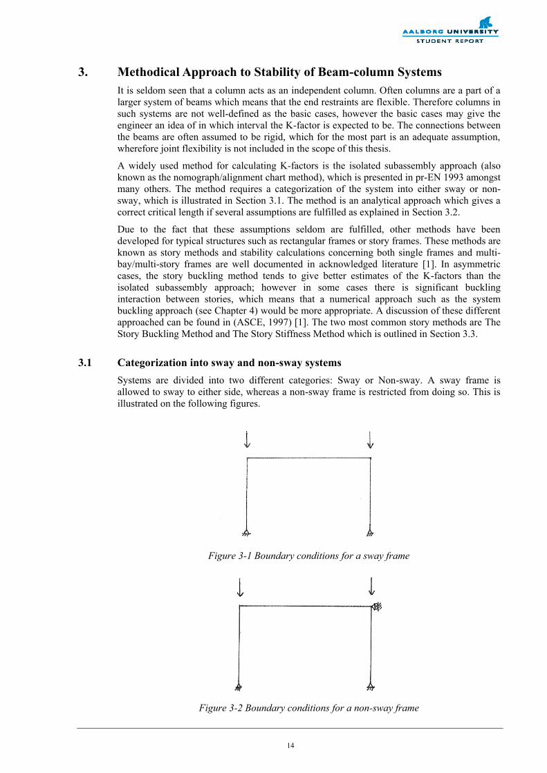
Figure 4-5 Model used for illustrating the influence of tension/compression in a member

adjacent to a column

The critical axial load is found by linear buckling analysis, and the corresponding K-factor for

varying horizontal load is shown in Figure 4-6. The reduction factor based on buckling

curve c and a yield stress of is shown in Figure 4-7.

Figure 4-6 K-factor at various axial force in adjacent horizontal member

28

Figure 4-7 Reduction factor according to EN-1993 at various axial force in adjacent

horizontal member

The main conclusions of these results are as follows:

1. When there are no axial force in the horizontal member, the K-factor is expected to be

in the interval , which is confirmed by the results where .

2. Applying tension in the horizontal member, the stiffness of the member is increased,

and therefore the rotational stiffness of the joint is increased leading to a lower K-

factor. The lower bound is approached for very high tensile force in the

horizontal member relative to the compressive force in the vertical member, where a

normalized horizontal force of will give a K-factor of . The mode

shape is in this case similar to the one of a single column fixed in one end and pinned

in the other (see Figure 4-8).

3. When the horizontal compressive force is equal to the vertical compressive force, the

horizontal member does not contribute to any rotational stiffness since the members

buckle with equal rotations at the ends (see Figure 4-9). This provides a K-factor of

one for both members.

4. When the compressive horizontal force becomes large compared to the compressive

vertical force, the K-factor is increased. This means that members in a system where

the axial compressive force goes towards zero, the critical length will go towards

infinity and thus the reduction factor goes towards zero. This is the paradox of the

system buckling approach.

29

Figure 4-8 Mode shape when tension in horizontal member is very large

Figure 4-9 Mode shape when compressive axial force is equal in both members

The influence of the load case is one of the reasons why determining K-factors for individual

members is challenging. Traditionally, engineers often think of the K-factor as dependent of

the system stiffness, but forget that the stiffness is load dependent.

The SBA provides a conservative way of determining the K-factors, which can be

implemented in FE-codes, however if more reasonable K-factors are needed the SBA is not

recommendable.

30

4.3.2 Verification of the K-factor Paradox

Using the same model as in previous section, it is shown how the large critical length for a

member with a small axial compressive force can be reduced without violating the structural

integrity.

It is legal to increase the axial compressive force in a member as long as it does not change

the system behavior significantly. If the additional force is increased to a level where the load

multiplier only is increased slightly, the critical length of the member with small compressive

axial force is reduced with only a slight increase in the critical length of members with large

compressive force.

In the model the horizontal load is kept constant and linear buckling analyses are performed

for various vertical loads. The critical load for each member is calculated using the SBA and

the corresponding K-factor is seen in Figure 4-10. The reduction factor based on buckling

curve c and a yield stress of is shown in Figure 4-11.

Figure 4-10 Calculated K-factors

Figure 4-11 Calculated reduction factor according to EN-1993

From Figure 4-10 and Figure 4-11 it is seen that a small axial force in the vertical member

leads to an unrealistic high K-factor and low reduction factor in this member. However, by

31

increasing the axial force in the vertical member the K-factor decreases significantly, while

only a small increase for the horizontal member is found.

In practice, this can be used to decrease the utilization ratio for the axial force in a member,

leaving more capacity for actions caused by moments. To demonstrate this, we consider an

extended version of the previous model. The horizontal member now has a geometrical length

of , and the load case is a horizontal load of acting on the middle of the vertical

column and a horizontal load of acting on the rigid joint (see Figure 4-12).

Figure 4-12 Model consisting of two members with small and large axial force respectively

A linear buckling analysis is performed and the mode shape and load multiplier is shown in

Figure 4-13.

Figure 4-13 First mode

32

As the axial force in the vertical member is small, the critical load and reduction factor

becomes small. In Table 4-3 results of sectional forces, reduction factors and utilization ratios

(UR) are listed. The yield stress is taken as and an elastic distribution is used. The

reduction factor is based on buckling curve c. The formulas used for calculating the

utilization ratio are given by:

(38).

and

(39).

where and are the sectional forces, is the section modulus, is the cross sectional

area and is the yield stress.

Member Load

multiplier Axial force

Reduction

factor UR

(Axial) Moment

UR (moment)

UR Total

Horizontal

Vertical

Table 4-3 Sectional forces, reduction factors and utilization ratios

It is found that the vertical member has a very low reduction factor and a utilization ratio

larger than . To increase the reduction factor, a fictive additional load is applied to increase

the axial force (and thereby the critical load) in the member. The additional load is taken as 10

times the real axial force in the vertical member and applied at the top of the column (see

Figure 4-14). Results are listed in Table 4-4.

Figure 4-14 Additional load applied at the top of the vertical column

33

Member Load

multiplier Axial force

Reduction

factor UR

(Axial) Moment

UR (moment)

UR Total

Horizontal

Vertical

Table 4-4 Sectional forces, reduction factors and utilization ratios after increasing the critical

load in the vertical member

The results show the paradox, that it is possible to decrease the utilization for one member by

applying extra load. However it has to be validated, that the added fictive load does not have

significant influence on the system behavior e.g. there are no noticeable change in the

sectional forces in the entire system besides the applied axial force.

The idea of using fictitious forces to decrease the K-factors for certain members with the

disadvantage of a minor increase for others has been presented in earlier work by Choi and

Yoo [7].

4.4 Iterative System Buckling Approach

The reason for excessively large K-factors when using the SBA (equation (37)) arises from

the assumption that all members reach their buckling limit when the system buckles. Since not

all members are close to their buckling limit when the system buckles equation (37) is only

valid for the most critical member. As shown in the previous section an increase in axial in the

weaker members only has a small effect on the system load multiplier. Choi and Yoo (2008)

uses this in an iterative procedure where the axial force in the compression members is

increased until an convergence criteria where the change in K-factor is sufficiently small is

fulfilled. This eliminates the paradox that small axial forces give excessively large K-factors

[7].

The most and least influential columns are to be determined by:

√

(40).

Where is the axial force in the member, is the modulus of elasticity and is the moment

of inertia.

The K-factor is expressed as:

√

(41).

where is the final increase in axial force calculated as the sum of incremental changes:

(

)

(42).

where the subscript and refers to the least and most influential columns respectively. For

an easy and stable iteration process, the terms and are assumed to be equal to 1.0 in

the first iteration step. The constant value of from this assumption is used in subsequent

iterations for simplicity.

The convergence criterion is defined as:

34

(43).

where is the iteration number and is convergence criteria ( =0.001)

4.5 Summary

In this chapter the significance of the load case is made clear. Furthermore the system

buckling approach is exemplified with the implication of excessively large K-factors. The

system buckling approach has the benefit that it is possible to calculate the K-factor for each

individual member by an algorithm, however overly conservative values of K-factor for

members with small axial force necessitate an improvement of the method.

For a simple system consisting of two members, it is shown that it is possible to reduce the K-

factor by adding more axial force in the member with a small axial force. This does only have

an insignificant influence on the load multiplier for the system. This is idea is used by Choi

and Yoo (2008) as they have proposed an iterative system buckling approach. This method

overcomes the K-factor paradox but lacks the possibility to be implemented in general

software codes as the results of the iterative procedure is sensitive to both the incremental

fictive force and the convergence criterion. This is also discussed in Appendix 3.

35

5. Proposed Method – The Energy Ratio Method

In this chapter the principals behind the Energy Ratio Method (ERM) is explained. The ERM

is a numerical method with close connection to the System Buckling Approach (SBA). The

difference between the ERM and the SBA is that the ERM circumvent the paradox of

members with small axial force having extremely large K-factors.

The ERM could be considered as an extension of the SBA, where the idea behind the ERM is

to account for the fact that all members in a system usually does not reach their individual

buckling limit simultaneously. In the SBA the load multiplication factor is applied to the axial

force of all compressive members (see Section 4.2), whereas the ERM uses a higher load

multiplication factor for the members in which buckling is less pronounced. To assess how

prone a member is to buckling, a ratio between stabilizing and destabilizing energy in the

member is used. The energy calculations are based on the mode shape and load multiplier

found from a linear buckling analysis. In Figure 5-1 the method is illustrated.

Figure 5-1 The difference between the system buckling approach and the proposed method

In the first section, the classical energy based stability considerations is presented. Known

analytical formulas are used to validate a numerical calculation of energy. In the following

sections, the philosophy behind the proposed method and formulas used for calculation of K-

factors is outlined. Furthermore examples are used to verify the proposed method and

illustrate the connection to the SBA.

5.1 Energy Based Stability Considerations of a Beam Member

The critical load of a beam member can be found by the considering the energy balance

between inner and outer work. Due to bending of the beam inner work is done in the form of

bending strain energy, which stabilizes the beam. The outer work is done by the applied load

multiplied the displacement, which is destabilizing for the beam. Analytical and numerical

methods for calculating the inner and outer energy are further explained by [3] and [10].

5.1.1 Analytical calculation of energy

In the calculation we consider a simply supported beam with length , axial direction and

displacement field . The beam is subjected to an axial load (positive in tension).

36

Figure 5-2 Column considered for energy calculation

At the critical load level, the internal and external energy is of equal size, where the internal

energy corresponds to the strain energy in bending given in terms of the curvature by:

∫

(44).

and the external energy is the work done by the force with the axial displacement given by:

∫

(45).

where the is the membrane strain. The beam only undergoes small displacements and the

membrane strain can be approximated by:

(46).

and the external energy becomes:

∫

(47).

Using the criteria:

(48).

the critical load can be found explicitly, and the solution is exact if the displacement field is

exact.

5.1.2 Numerical calculation of energy

When performing the linear buckling analysis, a subdivision of each member into 4 elements

is used. The internal and external energy in each member can be found as a summation of the

37

energies in each element belonging to the member in question. The internal energy in an

element can be found by:

(49).

And the external energy can be found by:

(50).

where is a vector containing the elements 6 nodal displacements from the mode shape

(translation in x and y direction and rotation about z axis) and is the load multiplier.

and are the elements local stiffness matrix and geometrical stiffness matrix respectively.

The internal energy is the bending strain energy, which is equal to the inner work. The

external energy produces the bending stiffness reduction and the energy is coherent with the

outer work.

The ERM is suitable for implementation in finite element codes, since the prerequisite linear

buckling analysis is performed as a finite element method. In this project a 2 node beam

element based on Bernoulli-Euler theory is used. A MATLAB script with a simple finite

element code has been written to make the examples that demonstrates the ERM. The script

can be found in Annex 2. Only 2D models are used to demonstrate the method to minimize

the scope of the script; however the method can be extended to 3D.

5.1.3 Verification of Energy Calculation

In this section the analytical calculation of the energies from formulas (44) and (47) are

compared to the ones calculated by the MATLAB script using formulas (49) and (50). The

comparison is made of a beam with square section. The beam is simply supported and has the

side length and length .

Analytical Calculated Energy

The mode shape of a simply supported beam during buckling has the form of a half sine. If the

center deflection of the beam is noted , the displacement field is given by:

(

)

(51).

and the first derivative is given by:

(

)

(52).

and the second derivative is given by:

(

)

(

)

(53).

The integrals can be solved by using the following formulas:

38

∫ ( (

) )

[

(

)

]

(54).

And

∫ ( (

) )

[

(

)

]

(55).

The center deflection of the mode shape is (found from the script in the

following), and by using either formulas (44), (53) and (54) or formulas (47), (52) and (55),

the analytical solution gives a total energy of:

(56).

Numerical Calculated Energy

A model of the considered beam is applied an axial load of , hence the load multiplier is

the critical load in newton. The model is seen in Figure 5-3 and the external and internal

energy is seen in Figure 5-4.

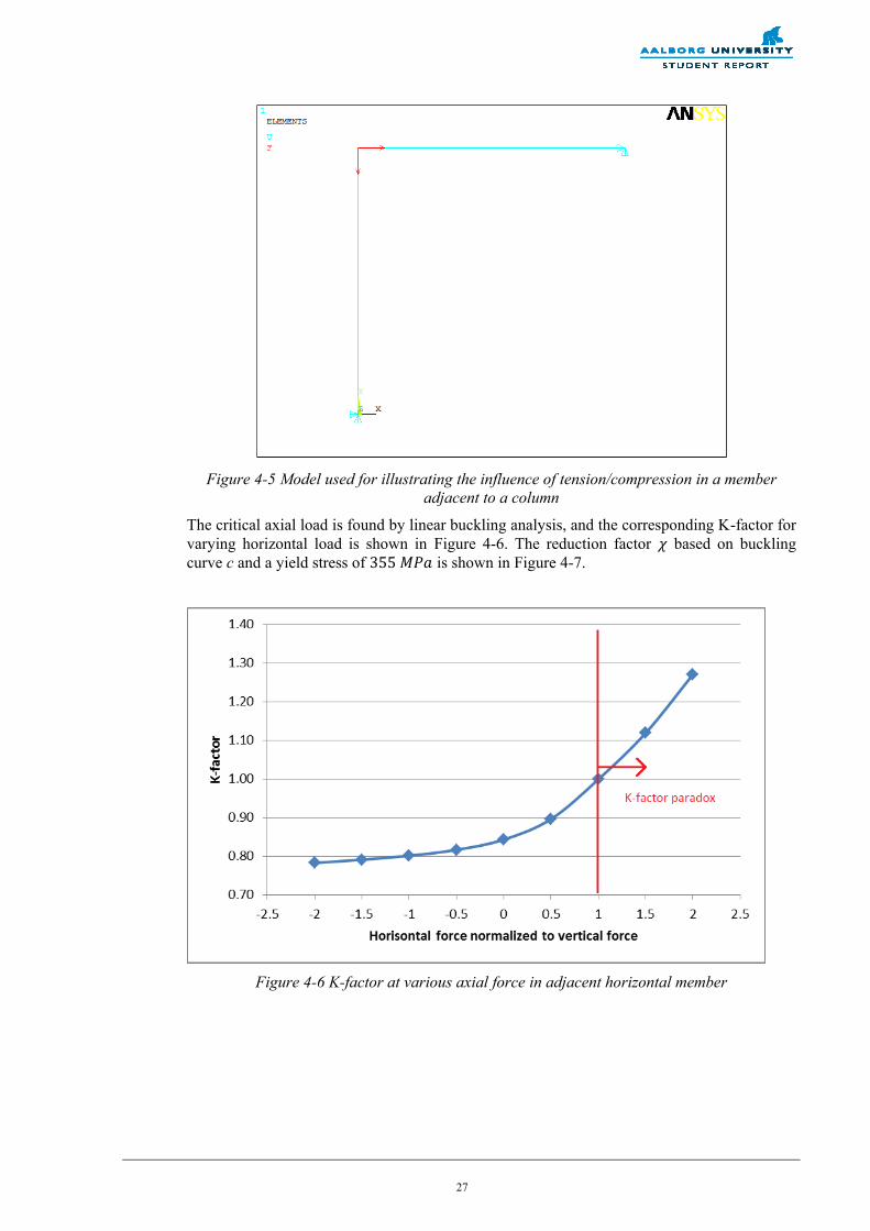
Figure 5-3 Model used for energy demonstration

39

Figure 5-4 Energy calculated numerical by MATLAB script

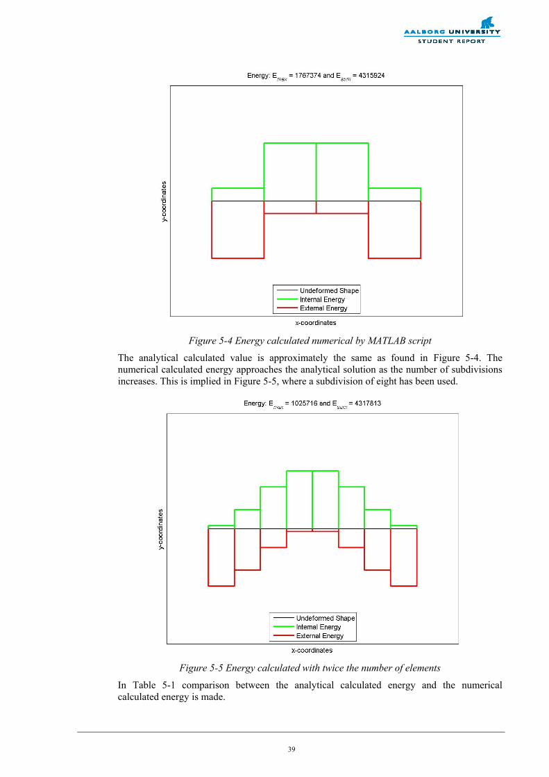
The analytical calculated value is approximately the same as found in Figure 5-4. The

numerical calculated energy approaches the analytical solution as the number of subdivisions

increases. This is implied in Figure 5-5, where a subdivision of eight has been used.

Figure 5-5 Energy calculated with twice the number of elements

In Table 5-1 comparison between the analytical calculated energy and the numerical

calculated energy is made.

40

Number of Elements Analytical value ERM value Deviation

4

8

Table 5-1 Comparison between analytically and ERM based energy calculations

It is assessed that a subdivision into four elements also is sufficient for the energy

calculations.

5.2 The Proposed Method

The K-factor of a column can be found by considering the stabilizing internal energy (which

is equivalent to the potential strain energy) and the destabilizing external energy (resulting

from the outer work done by the axial forces). The K-factor is derived from the critical load,

which is found from the criteria:

(57).

The calculation of the energy requires the buckling shape, which is known for the basic cases,

and when considering a system of members, the buckling shape is easily found by a linear

buckling analysis as the mode shape (see Section 4.1).

When performing the linear buckling analysis on a system of members, some members are

deforming as a result of the outer work being done by the axial force, and these members are

in a state of buckling. Other members are more in a state of bending due to rigid connections

to the members that are in a state of buckling. To assess “how much” a member is in the state

of buckling, the following energy ratio is being used:

(58).

The ratio is calculated for each member, and the member with the lowest ratio is

considered as the weakest member and therefore being 100% in the state of buckling. For this

specific member, the critical load is defined in the same way as in the SBA, which is:

(59).

where is the axial load in the member, and is the load multiplication factor found by the

linear buckling analysis.

The main point in the philosophy behind the proposed method is that for all other members,

the load multiplication factor is increased relative to the respective members energy ratio

compared to the lowest energy ratio. E.g. if a member has an energy ratio twice the size of the

lowest energy ratio, the load multiplication factor should be increased by a factor of two. The

lowest energy ratio is thereby a reference ratio, which is notated as and the critical load

for each member in the system can be determined as

(60).

Now the critical load for each element can be calculated using formulas (58), (60), (49) and

(50), and the K-factor for each element can be found using back calculations from the Euler-

formula given by:

41

(61).

Rewriting and inserting formula (60) yields:

√

√

(62).

In the special case where all members buckle at the same time, every member will have a ratio

of one, and the ERM gives the same result as the SBA.

This method eliminates the paradox from the SBA, and gives more reasonable K-factors for

all members in the system. However one must keep in mind that as for the SBA, the ERM

produces load dependent K-factors, and therefore the method should be used for each load

case when designing a structure.

5.3 Demonstration of the Energy Ratio Method

In this section the ERM is demonstrated. Comparison to the SBA is included to show the main

advantage of the ERM, namely that the paradox that relatively small forces provide large K-

factors in the SBA is avoided.

5.3.1 Simply Supported L-frame

In this example a model of an L-frame is used to demonstrate that:

When the members buckle at the same time, the ratio is equal to one for both

members.

The ERM provides the same results as the SBA for the member which is 100 % in the

buckling state, i.e. the one that has the lowest energy ratio .

The K-factors is in the expected interval for all load cases, thus excluding the paradox

from the SBA.

The model consists of two members with the same geometrical properties. The length of the

members is and the cross section is a square with side length . The supports allow

rotations but no displacement. The model is the same L-frame as used in Section 4.3 to

illustrate the paradox in the SBA.

The load cases considered is produced by letting the axial force in the vertical member

(Member1) be fixed at (compression), and then varying the axial force in the horizontal

member (Member2) as both compressive and tension. The model can be seen in Figure 5-6

where the axial force in Member2 is (compression).

42

Figure 5-6 Model produced by MATLAB script providing K-factors by both ERM and SBA

The result from various load cases is seen in Figure 5-7 and Figure 5-8, where the y-axis reads

the K-factor. The x-axis is the axial force in Member2 normalized to the axial force in

member1, which means that negative values are equivalent to tension in Member2.

Figure 5-7 K-factors for Member1 found by ERM and SBA

Figure 5-7 shows how the K-factor for Member1 becomes large in the SBA when the axial

force in Member 1 is small compared to the axial force in Member2, which is the paradox of

the SBA. The ERM provides better results where the K-factor is in the expected

interval . The lower bound of 0.7 is found when tension in Member2 goes

towards infinity, which prevent rotation at the rigid joint due to increased stiffness of

Member2. This is in accordance with the basic case of a beam fixed at one end and roller

supported at the other end (see Figure 2-2). In Figure 5-8 a zoom of Figure 5-7 is shown.

43

Figure 5-8 Plot of K-factors for Member1 in reduced interval of load cases

From Figure 5-8 it is seen that the ERM provides the same results of the K-factor for

Member1 as the SBA when the axial compressive force in Member1 is the larger than in

Member2. This is because the energy ratio is smallest in Member1, i.e. Member1 buckles

first, since the two members have the same properties and the force in Member1 is largest.

When the axial compressive force in Member2 becomes the largest, the K-factor for Member

1 decreases according to ERM. This is because Member1 in these load cases function more as

a stabilizing member by its bending stiffness, rather than a compressive member.

Furthermore it is seen, when the axial compressive force in both members is of same size, the

members buckle at the same time, which provides a K-factor of one for both members. This is

because each member focus all its internal energy on preventing buckling, leaving no bending

stiffness to prevent rotation at the rigid joint. Therefore the K-factor is 1.0 according to the

basic case of a beam which is simply supported at one end and roller supported at the other

end. In Figure 5-9 the model with equal axial force in the members is shown, where it is seen

that the energy ratio is one for both members.

Figure 5-9 Model showing buckling at the same time for both members

44

In Figure 5-10 the K-factor for Member2 is shown.

Figure 5-10 K-factors for Member2 found by ERM and SBA

From Figure 5-10 same conclusions for Member2 as for Member1 can be made. It shows that

the ERM provides the same results for the K-factor of Member2 as the SBA, when Member2

is the member that buckles first. Furthermore when the axial force in Member1 is largest the

ERM decreases the K-factor for Member2.

5.4 Other Application of the Energy Ratio Method

As illustrated in previous section, the energy ratios for each member in a system gives a

picture of which members that are mainly in a buckling state, and which members that acts

more as stabilizing member by their bending capacity.

Previous attempts to overcome the paradox in the SBA has been made by others, where

fictitious axial force are applied iteratively to initiate buckling at the same time for all

compressive members [7][8]. This method is a good alternative to the traditional SBA, where

the K-factor decreases for the members that act as stabilizing bending members. However the

method provides a larger K-factor for members which are most prone to buckling, because the

fictitious forces applied yields a lower load multiplication factor.

The ERM can be used as an iterative method to calibrate the axial force in the compressive

members so that the energy ratio becomes one for all members, i.e. buckling occurs at the

same time for all compressive members. As an example on this procedure the following

example is provided.

The model is an L-frame where Member1 has the length and a fixed support at the base,

and Member2 has the length and a simple support at the end. Both members have a

square cross section with side length of . The load case considered is an axial force of

in Member1 and in Member2. The model is seen in Figure 5-11.

45

Figure 5-11 Model used to illustrate iterative procedure to find same time buckling

By multiplying the energy ratio by the axial force in each member iteratively the energy

ratio in both members becomes one in two iterations. The model of the two iteration steps is

seen in Figure 5-12 and Figure 5-13. Note that in Figure 5-13 same time buckling occurs and

the energy ratios is equal to one.

Figure 5-12 First iterative step: Energy ratios approaches one

46

Figure 5-13 Second iterative step: Energy ratios have become one for both members

As an addition to this example, the difference between the traditional SBA, the iterative SBA

according to [7], and the ERM can be seen by comparing the K-factors found in Figure 5-11

and Figure 5-13. The K-factors are listed in Table 5-2 and it is seen that the ERM in this

example provides more realistic K-factors.

K-factors Traditional SBA

SBA

(same time buckling) ERM

Member1 0.57 0.70 0.57

Member2 3.61 1.00 0.75

Table 5-2 K-factors found by traditional SBA, improved SBA and ERM

The results from this example illustrates, that same time buckling and the SBA, in cases were

the system consists of all compressive members, may provide overly conservative K-factor for

the members that are in the buckling state. In cases were the system consists of both tension

and compression members the improved might give better results than the ERM from a design

point of view.

5.5 Summary

In this chapter, a method to avoid the paradox of the System Buckling Approach has been

proposed. The paradox, of members with relatively small axial force having excessively large

K-factors, is circumvented by considering members as acting partly as a compression member

and partly as a bending member.

Based on the mode shape found by the traditional linear buckling analysis, the internal and

external energy can be found in each member, and the energy ratio indicates whether a

member is stability sensitive to the load case. A low ratio means the axial forces is performing

a relatively large destabilizing outer work.

47

The one member which has the lowest ratio is considered as being 100 % critical in the given

load case, thus the load multiplier defines the critical load for member directly by

multiplication to the axial force in the member. This member is chosen as the reference

member, and the load multiplier is increased for the other members in the system by a factor

corresponding to the ratio between the energy ratio of the considered member and the

reference energy ratio of the member being 100 % critical. Thereby the critical load can be

found as:

(63).

The proposed method is easily implemented in traditional FE-codes, and the method is not

sensitive to extremely small axial forces.

48

6. Comparison of Proposed Method to Other Known Methods

In this example, the Energy Ratio Method is applied to a model of a three story building,

which has already been investigated by Choi and Yoo (2008) [7]. The proposed method of

Choi and Yoo is the aforementioned iterative System Buckling Approach (iSBA) (see Section

4.4), and in their example the method is compared to traditional SBA and story methods.

The purpose of this example is to compare the Energy Ratio Method to the other widely used

and newly proposed methods.

6.1 Model Description

The model of the three story building is a 2D frame consisting of vertical members (HEB360)

and horizontal members (IPE400). Both the HEB360 and the IPE400 has bending about the

strong axis, and sectional properties can be found in Table 6-1. The modulus of elasticity is

set to .

Sectional properties HEB360 IPE400

Moment of inertia

Sectional Area

Table 6-1 Sectional properties

The story height is , which gives a total height of , and the bay width is .

Concentrated loads are imposed on the joints of each story, where the load . The

horizontal loads shown with dotted arrows are only used in the story stiffness method. The

model is seen in Figure 6-1.

Figure 6-1 Model of the three story building

6.2 Results Compared to the Energy Ratio Method

In the paper presented by Choi and Yoo (2008) the story buckling method, the story stiffness

method, the method suggested by Gantes and Mageirou (2005) [12] and the system buckling

approach is compared to their proposed method: The iterative system buckling approach. A

vague method description has led to questions about the method; however it has been possible

to recreate the results from the paper (see Appendix 3).

49

The Energy Ratio Method (ERM) has been applied to the model and the results are included

in Table 6-2 with results from the paper of Choi and Yoo. Furthermore the results are plotted

in Figure 6-2, where the Energy Ratio Method is highlighted in red color.

K-factors Story 1 Story 2 Story 3

Story Buckling Method

Story Stiffness Method

Gantes & Mageirou

System Buckling Approach

Choi & Yoo (iSBA)

Energy Ratio Method

Table 6-2 Comparison of K-factors

Figure 6-2 Results graphically displayed

The ERM is calculated using a MATLAB script, where beam elements have rectangular cross

sections and is based on Bernoulli-Euler beam theory. In Appendix 2 it is verified that results

are independent on cross section type and only depends on sectional properties.

6.2.1 Similar Results Found by the ERM Compared to Other Known Methods

The results show the SBA paradox of the top stories having excessively large K-factors. It is

clear, that the other methods provide much more realistic results. The method proposed by

Choi and Yoo gives the most favorable results for story 2 and story 3; however it is on the

cost of some of the strength of story 1. This is related to the slight decrease in the load

multiplier. When only considering story frames with no axial compressive force in the

horizontal members, the proposed method by Choi and Yoo provides favorable results,

however if there is a relatively small axial compressive force in the horizontal members the

applied fictitious forces will tend to decrease load multiplier significantly. This would lead to

conservatively large K-factors for the vertical members in story 1. One of the strength of the

ERM is that it is provides intuitive realistic K-factors for all members in the structure. E.g. if

50

an axial compressive force of where applied to the horizontal members the vertical

members would get a non-noticeable increase in the K-factor and the horizontal members

would be assigned a K-factor of approximately .

6.2.2 Inconsistent Results Found by the ERM Compared to Other Known Methods

The ERM stands out in the result by the fact that it provides a larger K-factor for Story 3 than

for story 2. It is assessed, that this is caused by the fact that the internal strain energy becomes

relatively smaller in story 3 than story 2 because of the relative transverse displacement of

each story seen in the mode shape (see Figure 6-3). This effect is also indicated when

comparing the Story Buckling Method to the Story Stiffness Method (see Table 6-2), where

the decrease of the K-factor is small by the Story Stiffness Method, because it considers the

transverse displacements.

Figure 6-3 Modeshape of three story building where axial load increases down the columns

The main difference in sway when the axial load increases down the columns compared to a

constant axial load is emphasized in another example by Choi and Yoo, where a seven story

three bay frame is considered (see Figure 6-4). Note the increase (marked with red circle) in

the K-factor from story 6 to story 7 in load case 2 is found by the story stiffness method.

51

Figure 6-4 Example from Choi and Yoo (2008)

6.3 Summary

This example illustrates how the ERM provides realistic K-factors in accordance to known

analytical methods. Furthermore it has been noted, that the method is not sensitive to

members with relatively small axial force, wherefore the method is suitable for

implementation in FE-codes.

52

7. Conclusion

The critical length is a key parameter when designing compressive members according to the

Eurocode. Most engineers have a reasonable idea of, in which interval the K-factor is

expected to be, however as the complexity of the structures increases the risk of incorrect

stability assessment becomes imminent.

New structures are often designed with some degree of spare capacity, therefore exact K-

factors are not that crucial, however the risk of overlooking a general behavior, that yields

larger K-factor than expected, could lead to a disastrous design. This can be avoided by

performing a linear buckling analysis, which will show the general behavior of the system.

When existing structures are reassessed because of change in the anticipated load exposure or

design safety, some members might become over utilized according to the design formulas.

By evaluating more accurate K-factors than previously conservative values, one might avoid

the need to strengthen the structure.

Analytical correct K-factors are seldom obtainable, wherefore methodical approaches are

widely used to give estimates of K-factors. These methods can provide realistic K-factors in

typical structures such as story-frames, but due to various assumptions in the methods the

usability is primarily limited to regular frames.

In complex structures where methodical approaches cannot be used, numerical approaches

like the system buckling approach are useful. The method provides an exact solution of the

member most prone to buckling, however for members with a low axial force that acts mainly

as stabilizing bending members the method yields excessively large K-factor. This is a known

paradox and the reason why, the method is not implemented as an automatically

determination of K-factors in code check software.

The main objective of this thesis was to propose a method that overcomes the paradoxical

weakness of the system buckling approach. The proposed method is based on energy

considerations, where the load multiplier from a linear buckling analysis is weighed to the

individual members. It was found that method provides realistic K-factors that are not subject

to the paradox of the traditional system buckling approach.

The proposed method is deduced from physical arguments, where the energy balance between

inner and outer work is used as an indicator for how much the individual members are

sensitive to additional load in the critical state. Only 2D verification of the method was

performed, however further thorough investigation and application of the method is believed

to have the potential of the development of a method, which can be implemented with into

code check in existing code check software.

53

References

[1] ASCE. (1997). Effective length and notional load approaches for assessing frame

stability. ASCE Technical Committee on Load and Resistance Factor Design. New

York. USA.

[2] Bazant, Z. P. and Cedolin, L. (2010). Stability of structures. World Scientific

Publishing Co. Pte. Ltd. Singapore.

[3] Bonnerup, B and Jensen, B. and Plum, C. M. (2009). Stålkonstruktioner efter DS/EN

1993. Nyt Teknisk Forlag. Copenhagen. Denmark.

[4] Canle, R. (1999). “The Effective Length of Columns in Unbraced Frames with more

than one story and Pinned Bases”. Unpublished.

[5] CEN. (1992). prEN1993-1-1:1992 Design of Steel Structures - Annex E. European

Committee for Standardization. Brussels. Belgium.

[6] CEN. (2009). DS/EN 1993-1-1:2009AC Design of Steel Structures. European

Committee for Standardization. Brussels. Belgium.

[7] Choi, D. and Yoo, H. (2008). “Iterative system buckling analysis, considering a

fictitious axial force to determine effective length factors for multi-story frames”.

Engineering Structures. 31. pp.560-570.

[8] Choi, D and Yoo, H. (2009). “Improved system buckling analysis of effective lengths

of girder and tower members in steel cable-stayed bridges”. Computers and Structures.

87. pp.847-860.

[9] Choi, D and Na, H. et al. (2010). ”Iterative Eigenvalue Analysis for Stability Design of

Three-dimensional Frames Considering a Fictitious Axial Force Factor”. International

Journal of Steel Structures. 10(4). pp.325-335.

[10] Cook, R.D et al. (2002). Concepts and applications of finite element analysis. 4th

edition. John Wiley & Sons Inc. USA.

[11] Damkilde, L. (1998). ”Stabilitet af rammer – Derformationsmetoden”. Institut for

Bærende Konstruktioner og Materialer. Danmarks Tekniske Universitet. Denmark.

[12] Gantes, C. J. and Mageirou, G. E. (2005) “Improved stiffness distribution factors for

evaluation of effective buckling lengths in multi-story sway frames”. Engineering

Structures. 27(7). pp. 1113-1124.

[13] Julian, O. G. and Lawrence, L. S. (1959). Notes on J and L nomographs for

determination of effective lengths. Jackson and Moreland Engineers. USA.

[14] Timoshenko, S. P. and Gere, J. (1961). Theory of elastic stability. 2nd edition. McGraw-

Hill Book Company Inc. New York. USA.

[15] Wood, R.H. (1974). “Effective Lengths of Columns in Multi-Story Buildings”. The

Structural Engineer. 52. p. 341-346.

I

APPENDIX 1

Examples of Methodical and Experience Based Approaches

II

1. Example 1: Offshore Bridge between Gorm C and Gorm E

An often used type of offshore bridge consists of three chords and a system of braces. A

cross section of this type of bridge forms a triangle, where some bridges are orientated with

the apex chord upwards as the bridge between Gorm C and Gorm E (see Figure 1-1), and

some are turned upside down.

Figure 1-1 Typical offshore bridge between Gorm C and Gorm E in the North Sea.

The bridge between Gorm C and Gorm E has a span of 102.5 m. The chord in the apex has a

larger cross sectional area than each of the two chords carrying the deck. The braces have the

largest cross sectional area at the ends of the bridge and smallest at the middle, which is

logically chosen when thinking of the shear distribution of a uniform loaded beam.

In the present example the choice of critical length for the chords and braces in the bridge is

discussed. Appropriate default values, which have been used for the actual design of the

bridge, are outlined and a linear buckling analysis of a beam model is used for comparison.

To see the difference between this type of bridge having the apex chord in the top or bottom,

the same linear buckling analysis is performed were the beam model is turned upside down.

The purpose of this example is to:

Validate the use of empirical K-factors on the members that are most prone to

buckling.

Illustrate that in some cases the general behavior with a global sway mode becomes

determinative for the buckling capacity, so that the use of empirical K-factors for

individual members no longer applies.

1.1 Empirical Values of K-factor for Calculation of the Critical Length

For the design of the bridge empirical default values of the K-factor have been used. All

chords are assigned a K-factor of 1 and all braces are assigned a K-factor of 0.7. These

values can be found in the FEM package ROSAP, which was used for the design of the

bridge.

1.2 Description of Beam Model

The geometry is modeled according to the structural drawings found in Annex 1.

III

The support conditions of the bridge is pinned in one end (no displacement but rotations

allowed in all directions) and roller supported at the other end of the two deck chords (same

as pinned but displacements allowed in the bridge direction).

Point loads is applied the keypoints connecting braces to the two deck chords. This

represents a uniform load distribution, which is typical for an offshore bridge.

The model of the bridge is shown in Figure 1-2 and Figure 1-3 orientated normally and

upside down respectively.

Figure 1-2 Beam model of the bridge between Gorm C and Gorm E.

Figure 1-3 Beam model of the bridge turned upside down.

IV

1.3 Results from buckling analysis

In the buckling analysis it is found that the first and second mode in principle has the same

deformation pattern. The difference in the two modes is the direction in which the

deformation happens. The load multiplier for the first and second mode is and

respectively. In Figure 1-4 and Figure 1-5 the two modes are seen.

Figure 1-4 First mode. Apex chord deforming in the horizontal plane.

Figure 1-5 Second mode. Apex chord deforming in the vertical plane.

V

To see the distinct deformations the second mode is chosen to be seen from the side (see

Figure 1-6).

Figure 1-6 Side view of the second mode shows distinct deformations of the chord and

braces.

It is noted that the most slender braces furthest from the middle receives the largest

deformations. This indicates that critical stress level is reached first in these elements when

the load is gradually increased. Also deformations of the apex chord are significant, which

indicates that the stress level is close to the critical at the time when the brace buckles. In the

following, axial forces in the aforementioned braces and chord at the critical load level are

compared to the critical axial forces calculated from default critical lengths. The load

multiplier of is used and results are given in Table 1-1.

Critical Axial Force Axial Force in element at

critical load level

Critical axial force calculated from

default critical length

Deviation

Brace (largest

deformation)

Chord (middle of the

bridge)

Table 1-1 Comparison of critical load level to critical axial forces determined by default K-

factors.

It is assessed that the large deviation at the brace is due to a conservatively taken default

value of the K-factor. If the K-factor is calculated backwards from the axial force in the

braces at the critical load level, a value of is found. Compared to the default value of

it seems so that the element boundary conditions is closer to a column fixed in both ends.

This is in agreement with the fact that the brace buckles before the chord, wherefore the

rotational stiffness is high at the brace ends. The default value of 0.7 insures the situation

where the load in the brace and the chord reaches a critical level at the same time, which

allows rotation at one of the brace ends.

When using empirical values it is important to assess if it is reasonable values. In this case

the position of the keypoints connecting the braces to the chords is fairly fixed in the

buckling modeshape, since the chord in compression (the apex chord) is maintained by

VI

braces in two transverse directions. This means that the general behavior is not determinative

for the buckling capacity, and therefore K-factors between and is expected according to

the basic cases (see Figure 2-2 section 2.1 of the main report). In the following section a

hypothetical situation where the bridge is turned upside down is analyzed to emphasize when

care should be taken.

1.4 Upside Down Bridge

When turning the bridge upside down the deck chords are in compression. The keypoints at

the deck chords are not fixed if the bridge has a global mode shape corresponding to a

horizontal transverse deformation of the deck. Therefore the bridge may fail by buckling at a

lower load level than expected when using default K-factors. In Figure 1-7 the first

modeshape of the upside down bridge is seen.

Figure 1-7 First mode of the upside down bridge.

The same comparison of the K-factor as in section 1.3 is made in Table 1-2 for the first

modeshape.

Critical Axial Force Axial Force in element

at critical load level

Critical axial force

calculated from default

critical length

Deviation

Brace (largest

deformation)

Chord (middle of the

bridge)

Table 1-2 Comparison of critical load level to critical axial forces determined by default K-

factors.

The same conclusions as in section 1.3 concerning the K-factor can be made. However the

deviation for the brace is smaller, because the ratio is closer to (see Table 1-3). The

ratio is given by:

VII

where is the ratio of the axial force in the chord and brace, and is the ratio of the

critical axial force for the chord and brace. If the elements buckle at the same time

with element boundary conditions corresponding to the K-factors used for calculating the

critical axial forces. Comparison of the ratios can be seen in Table 1-3.

Ratio table Axial force ratio

chord/brace

Critical force ratio

chord/brace

Total ratio

Bridge normally orientated

Bridge turned upside down

Table 1-3 Comparison of ratios for assessment of sametime buckling of chord and brace.

The first modeshape did not show the global sway modeshape with a low critical level, but

the modeshape appears as the second mode (see Figure 1-8).

Figure 1-8 Second mode of upside down bridge. Global modeshape with keypoints deformed

out of initial position.

The second modeshape shows a global modeshape where the keypoints is deformed out of

initial position. However the deck chords and deck braces provides enough stiffness so the

global sway modeshape is not the first critical mode. If the bridge deck is narrowed to half

the width, a load multiplication of is found (see Figure 1-9), which gives a

considerable lower critical load level than the first mode in Figure 1-7.

VIII

Figure 1-9 Narrow bridge with a global sway modeshape at a low critical level.

1.5 Summary of Example 1

Using the linear buckling analysis on a beam model of the bridge between Gorm C and

Gorm E the default values of K-factors for chords and braces is explained. The risk of global

sway modes is clarified with an upside down narrow version of the bridge that gives a low

critical load level. A general behavior with a global sway modeshape might be overlooked

by the designing engineer, however the linear buckling analysis provides an effective check

of this, so that unstable designs can be avoided.

IX

2. Example 2: Support Structure for Galleries

The support structure for this gallery is an example of an uncommon structure where the

general behavior of the system is hard to predict. The support structure consists of I-profile

beams while the bracing is made with tubes. The structure is characterized by being slender

and unbraced in one plane and thick and semi brace in the other.

In the following the subassembly method is used to evaluate the stability of the structure and

the results are compared to a linear buckling analysis. Furthermore common engineering

practice is used by simplified assumptions.

Figure 2-1 Support structure for galleries

2.1 Isolated Subassembly Approach

Based on the pre-EN1993 standard described in section 3.2 of the main report the critical

column length for the straight bottom column is calculated using the isolated subassembly

method.

The column is a HEB340 as sketched on Figure 2-2 with the weak axis out of plane.

Based on the structure, it is assumed that the column is well braced about its weak axis,

which means a critical column length about the weak axis with a value between and 1

times the actual length. The value of 1.0 is chosen. This simplification was made in the

original design.

X

Figure 2-2 Column designations

The column is simple supported at the bottom which means , and are equal to

zero. This also applies to . The value of effective beam stiffness is calculated based

on the most conservative approach as described in section 3.2 of the main report. The

horizontal beam and the top column are also HEB340 profiles.

(64).

(65).

(66).

(67).

(68).

Using the formula for sway mode the following K-factor is obtained.

[

]

(69).

To sum up the following K-factors are found using a conventional way of establishing

critical lengths: and

XI

2.2 ANSYS Model

In order to perform a linear buckling analysis of the structure a model is build up in ANSYS

APDL.

The structure is simply supported at the bottom and this is sketched on Figure 2-3.

Figure 2-3 Support structure for galleries

Two point loads of each in the vertical direction are applied to the joints shown on the

figure below.

Figure 2-4 Application of loads

A buckling analysis is performed and the load multiplier and axial force of the column is

outputted.

XII

Load multiplier

Axial force

Table 2-1 ANSYS Output for first buckling mode

The corresponding mode shape is shown in the following figures.

Figure 2-5 First buckling mode - front view

Figure 2-6 First buckling mode - side view

The output gives a critical load for the column, and based on this load, the critical column

length for the found buckling mode is derived.

(70).

XIII

Critical length about the weak axis:

√

√

(71).

In order to calculate the critical column length about the strong axis the buckling mode with

the lowest multiplier corresponding to this deflection is found. This is the case with the third

buckling mode as shown on the figures below.

Figure 2-7 Third buckling mode - front view

e

Figure 2-8 Third buckling mode - side view

XIV

Load multiplier

Axial force

Table 2-2 ANSYS Output for third buckling mode

This gives a critical buckling load of:

(72).

The critical column length about the strong axis can then be calculated as:

√

√

(73).

2.3 Comparison of Isolated Subassembly Method and ANSYS

In the following chart the results from the two methods are summarized.

Isolated

Subassembly ANSYS Deviation

Weak axis

Strong axis

Table 2-3 Comparison of -factors

About the weak axis the assumption that the column was well braced, and therefor has a

critical column length of one times the actual length of column turns out to be non-

conservative. When used in further calculations to determine the load capacity, the ANSYS

critical length gives a reduction factor and the prEN1993 gives .

About the strong axis the difference is much larger. A K-factor of , as found by the

subassembly approach, seems to be a very conservative value. This is partly due to the fact

that the structure is semi-braced against sway at the very top of the structure. This means that

the overall sway mode is a mix between non-sway and sway. This is not accounted for in the

method. By looking at formula (67) and (68) it becomes apparent that the only way to reduce

the critical length is to maximize the value of and minimize the value of . It can be

argued that the value of should be reduced as the resistance against rotation at the top by

default is assumed fixed. Reducing the value of and maximizing the value of would

at best give the following distribution factors.

(74).

The distribution factor gives a -factor of which is still larger than the obtained

ANSYS value of . This supports the claim that the method does not scale to this type of

problem where the structure is a mixture of sway and non-sway.

An alternative way of calculating the critical length of the bottom columns is to see the

bottom frame as an isolated frame, thereby assuming that the structure above doesn’t have

XV

any influence on the motion of the bottom frame. This means that the and in formula

(67) are equal to zero. By calculating formula (67) and (68) the following distribution factors

are obtained:

(75).

(76).

Thereby the K-factor becomes:

[

]

(77).

So by using this alternative approach to calculating K-factor a value of is obtained. This

value is closer to value from the buckling analysis but still higher. This is again because of

the semi braced nature against sway at the top of the structure.

In the table below the reduction factors, , about the strong and weak axis for both isolated

subassembly method and ANSYS is calculated. The reduction factor for strong axis buckling

for isolated subassembly is based on the lowest value of found using the alternative

approach.

Reduction factor Isolated

Subassembly ANSYS

Strong axis

Weak axis

Table 2-4 Summary of reduction factors

It quickly becomes apparent that estimating the critical column lengths can lead to either too

large or too small values. This is primarily due to the fact that the general behavior of the

system becomes hard to predict with the increasing complexity. Furthermore it should be

noted the results found in ANSYS using the linear buckling analysis only is valid for the

current load case, whereas the isolated subassembly method provides a K-factor that does not

depend on the load case.

2.4 Summary of Example 2

In this example the K-factor has a large variation based on the method used.

When using the isolated subassembly method from prEN1993 it is found that the largest K-

factor is about the strong axis. A linear buckling analysis in ANSYS shows the same, but

with different values.

In this case the isolated subassembly method from preEN1993 is overly conservative with a

reduction factor lower than what system buckling approach in ANSYS suggests.

XVI

APPENDIX 2

Verification of Cross-section input for 2D Elements in Strain Energy Calculations

XVII

1. Verification of Cross-section Type Independence

This appendix contains a comparison between a rectangular cross section using Bernoulli-

Euler beam theory and an I-profile cross section using Timoshenko beam theory. The point

of which is showing that the type of cross section, i.e. rectangular and I-profile, provides the

same result for the energy calculations as long as the area and moment of inertia are

identical.

1.1 General model

The frame is a three story frame. The columns are HEB360 and the horizontal girders are

IPE400. The frame has a total height of 30m and a width of 20m. The frame is simply

supported at the base and a load of 1 N is placed at each story.

Figure 1-1 Three story frame

The sectional properties are listed in the table below:

HEB360 IPE400

Area

Moment of inertia

Table 1-1 Sectional properties

1.2 2D Frame

The 2D model is based on beam elements with a rectangular cross section with the sectional

properties of an I-profile about its strong axis.

This gives the following result:

XVIII

Figure 1-2 Buckling analysis of 2D frame

1.3 3D Frame

The 3D model is based on beam elements with the I-profile cross section. As this model has

additional degrees of freedom further constraints are needed in order to obtain the same

system behavior as the 2D frame. This means supporting against rotation about the X

(torsional) and Y (out of plane) axis at the base of the frame.

The relevant modeshape is seen at modeshape number 5 as this model has different sectional

properties based on the direction of the cross section.

Figure 1-3 Buckling analysis of 3D frame

XIX

1.4 Comparison of 2D and 3D

The outputs considered in this report are the load multiplier and the stain energy (internal

energy). Therefore these two outputs are compared. The strain energy for the lower column

is summarized for the comparison.

2D Frame 3D Frame Deviation

Load multiplier 326518 321380 1.6 %

Strain energy 7654 7763 -1.4 %

Table 1-2 Comparison between 3D and 2D elements

The deviation is ascribed to the difference between Bernoulli-Euler and Timoshenko beam

theory, as the 2D frame is based on Bernoulli-Euler elements and the 3D elements is based

on Timoshenko elements. This is also described in section 4.1.2 is the main report.

XX

APPENDIX 3

Critics of Iterative System Buckling Approach

XXI

1. Critics of the iterative system buckling approach

This appendix contains critics of the iterative system buckling approach proposed by Choi

and Yoo [7]. The example used as reference example in the original article is used, as the

results of the article are tried replicated. The method description is vague in a few essential

key points, where assumptions concerning the explanation have been made.

1.1 Application of iterative system buckling approach

The model is a three story one-bay frame, with a width of 20m and a story height of 10m.

The columns are made of HEB360 and the girders are made of IPE400. A point load,

, is applied at the joints of story. The frame is pinned at the supports and a

modulus of elasticity of is used. The element properties are listed in the table

below.

HEB360 IPE400

Moment of inertia

Area

Table 1-1 Member properties

Figure 1-1 Reference example - 3 story one-bay frame

On Figure 1-1 the frame with member designation can be seen. A conventional system

buckling approach is made using ANSYS. A load multiplier is found and the

results are summarized in the table and figure below.

XXII

Figure 1-2 Result of linear buckling analysis

Member Axial force Critical

load

K-factor

1 and 9 (story 1)

2 and 8 (story 2)

3 and 7 (story 3)

Table 1-2 Results of system buckling approach

To determine the most and least influential member the stiffness parameter is calculated as:

√

where is the actual length of the member, is the axial force in the member, is the

modulus of elasticity and is the moment of inertia.

In Table 1-3 the calculated stiffness parameters are listed.

Member Stiffness

parameter

1 and 9 (story 1)

2 and 8 (story 2)

3 and 7 (story 3)

Table 1-3 Stiffness parameters for story 1-3

XXIII

It is assumed that the determination of the most and least influential member should be taken

amongst the compressive member. If the girder were included, the axial force of zero would

lead to a K-factor of infinity. This would give implications in the following calculation of the

increment of the fictitious axial force. Therefor the most influential member is Member 1

and the least influential is Member 3.

The method description is clear up to this point, but the explanation of the next step becomes

unclear. The increment of the fictitious axial force is to be determined as:

(

)

where subscript “mi” and “li” indicates the most and least influential member respectively.

is the K-factor found from the elastic buckling analysis and is the modified K-factor found

from the iterative elastic buckling analysis.

The unclearness in the article is that the iterative elastic buckling analysis have not yet been

performed wherefore does not exist. This is also seen in the flowchart from the article (see

Figure 1-3).

Figure 1-3 Flowchart of iterative system buckling approach [7]

In the iteration scheme is the iteration number and is the member number. It is seen that

is calculated for and not for because that is the conventional buckling

analysis. However an extract from [7] reads:

XXIV

Figure 1-4 Extract from article

As no further description is made it is assessed that should be taken from the

conventional buckling analysis ( and is calculated from a buckling analysis where

the loads have been increased by:

(

)

Since the members have the same properties the first increase becomes:

The modified K-factor for the least influential member is then calculated as , and

from the conventional buckling analysis we have . The increment in axial force

in the other members for the subsequent iterations is:

(

)

For every iteration step the following criteria is checked for all members:

where is a convergence limit. For members where the iteration criterion is met, no

more increments of fictitious axial force are added. It is not clear in the method description

whether or not to store the K-factor for each member in the specific iteration step where

convergence for the member is met, however this is assumed since the K-factor for story 1

(Member 1 and Member 9) becomes very large.

When performing the iterations convergence for all members is met at , and the

results are seen in Table 1-4.

Member Recreated

results of K-

factors

Results of K-

factors from

[7]

Deviation

[%]

1 and 9 (story 1)

2 and 8 (story 2)

3 and 7 (story 3)

Table 1-4 Results of the recreation of results from [7]

The description of the method is vague, however recreation of the results has been possible

with some assumptions to the method description. The deviations in Table 1-4 might

originate in rounding of properties and/or the programs choice of beam theory.

To sum up, the essential doubtful key points where:

XXV

Which value is assigned for ?

Should the K-factors for each member be taken in the iteration step where the

convergence criteria is met for the single member, or should the K-factor be taken in

the final iteration step where all members has converges?

1.2 Comments

In Table 1-5 K-factors is seen where the iteration scheme has been performed with a higher

and lower increments of the fictitious axial force .

Increment 1 and 9 (story 1) 2 and 8 (story 2) 3 and 7 (story 3)

Table 1-5 Results of K-factors with various iteration step size

The results from Table 1-5 shows that increasing the increment of fictitious axial force

provides lower K-factors for story 2 and story 3, however this is at the expense of a higher

K-factor for story 1. If the increment becomes too large, the results show non-consistency

which depends on the convergence criteria. If the increment is too small, the convergence

criteria might be met before an actual convergence is reached.

It should be noted that results also depends on the criteria . In Table 1-6 K-factors

has been listed where the criteria is reduced. The increment of has been used in

these calculations.

Criteria 1 and 9 (story 1) 2 and 8 (story 2) 3 and 7 (story 3)

Table 1-6 Results of K-factors with different convergence criterion

The results from the method proposed as described in the article are very much dependent on

the increment in fictitious axial force and convergence criteria. Even though results that

match those of the article are obtained, the method is hard to implement and use on other

examples, the results vary greatly depending on the combination of criterion and step size.

In later published articles [8][9] the method is slightly changed, which again would lead to

different results. The changes will not be outlined since the example used for comparison

only appears in [7].

XXVI

APPENDIX 4

Journal Paper (DRAFT)

1

Energy modified system buckling approach for flexural stability design of general beam systems

Mortensen, Jacob S1)+2), Hansen, Mikael1)+2) and Damkilde, Lars1)

1) Department of Civil Engineering, Aalborg University, Niels Bohrs Vej 8, DK-6700 Esbjerg, Denmark 2) ISC A/S, Borgergade 70, DK-6700 Esbjerg, Denmark

Abstract When determining the effective length of a column in a general beam system, the system buckling approach is the

most common method used. The system buckling approach does however yield excessively large K-factors for members with a relatively small axial force. This paper illustrates a new method that overcomes this paradox by modifying the system load multiplier for each member based on energy considerations. The method distinguishes between members being prone to buckling and those that are not sensitive to additional axial load. The method is verified by comparing results from the proposed method with results from previously known methods used on frames. The results show the proposed method gives reasonable effective lengths for all members in the frames. The proposed method’s prerequisites are already calculated for the linear buckling analysis which makes the method eligible to be included in software algorithms. Keywords: flexural buckling, effective length, system buckling approach, energy, excessively large K-factors

1 Introduction Almost all structures consist of compression

members which mean a risk of instability. Instability is a non-linear phenomenon, which often can be handled with linear considerations. In the European standards, a stability check often comprise of a check of the individual members, where the non-linear behavior is included by a reduction depending on the elastic critical load (CEN, 2009). The critical length of the compression member is needed, as it defines the critical load (Timoshenko, 1961). The critical length can be determined in a number of ways, either by methodical desk calculation or computer based methods. Most desk calculation methods are based on a number of assumptions in order to obtain an analytical solution. The isolated subassembly approach considers the rotational stiffness among adjacent members, but assumes all members have the same stiffness parameters and therefore buckles at the same time (ASCE, 1997). Gantes and Mageirou have developed a more comprehensive approach considering all rotation and translation at the beam ends. This approach yields good results for frames (Gantes and Mageirou, 2005). The story-methods allows for shear to be transferred between columns in a story, which means that the weaker columns are supported by the stronger ones. But this method suffers from the same assumptions depending on how the critical load is calculated (ASCE, 1997). It also means that these methods are made for specific cases, which for the most part mean regular frames. Therefor the usability of these methods is limited.

When evaluating structures that cannot be classified as a regular frame by a number of stories and/or bays, the critical length are either determined by experience and standard values or by computer based numerical calculations such as a system buckling analysis (ASCE, 1997). As personal computers are a basic tool for the engineer, analysis such as a system buckling analysis becomes more common. The system buckling analysis is not limited to specific cases and therefor offers a wide usability. The system buckling analysis assumes that all members reach their buckling limit when the system buckles, this leads to the paradox that compression members with a small axial force will give excessively long critical lengths. This means that the method is often used as a supplement to the analytical approaches. A new method has been proposed where a fictitious axial force is used in an iterative manner in order to assess this problem (Choi and Yoo, 2008, 2009, 2010). The results of this method do however rely on the increment in fictitious force and the convergence criterion of the iteration process. In this paper, a new method based on the system buckling analysis is proposed, which is easily programmable into existing software. The method uses a modified load multiplier for each member based on their individual buckling resistance calculated using energy considerations. In order to verify the proposed method the K-factors are calculated for different cases and compared to results from numerical methods and analytical methods where relevant.

2

2 Current Methods The K-factor is defined from the Euler load:

𝑁𝑐𝑟 =

𝜋2 ∙ 𝐸𝐼(𝐾 ∙ 𝑙)2 => 𝐾 = �

𝜋2 ∙ 𝐸𝐼𝑁𝑐𝑟 ∙ 𝑙2

(1).

The critical load can be determined analytically using the beam-column differential equation assuming all end restraints are well defined. This is easily done for the commonly known end restraints just as pinned and fixed. When a column is a part of a larger system of members the end restraints depends on the behavior of the entire system. This means that a column acting in a system needs to have defined four different restraints, as seen on Figure 1, in order to obtain an analytical solution.

Figure 1 General column restraints

Determining these end restraints are often a cumbersome process and several methodical approaches are often used instead.

2.1 Isolated Subassembly Approach The isolated subassembly approach is a commonly

used approach for determining K-factors for a single column. It is also known as the alignment chart method, G-factor method or nomograph method. The method is characterized by the determination of stiffness factors, or G-factors, at each end of the column. The stiffness factor is a function of the adjacent beams stiffness coefficients. The stiffness factors at each end of the column are used in junction with either an alignment chart, nomograph or approximated formulas. These are based on a number of assumptions which must be fulfilled in order to obtain correct results (ASCE, 1997). Based on the origin of the method the stiffness factors can be calculated in a number of ways, where the European pr-EN1993 standard uses the following equations (CEN, 1992):

𝜂1 =𝐾𝐶 + 𝐾1

𝐾𝐶 + 𝐾1 + 𝐾11 + 𝐾12

(2).

𝜂2 =𝐾𝐶 + 𝐾2

𝐾𝐶 + 𝐾2 + 𝐾21 + 𝐾22

(3).

where 𝐾𝐶 is the column stiffness coefficient, 𝐾𝑖 are the stiffness coefficients for the adjacent columns and 𝐾𝑖𝑗 is the effective girder stiffness coefficient. Based on the state of sway the K-factor can be obtained as:

Non-sway mode:

𝑙𝑠𝑙

= 𝐾 = �1 + 0,145 (𝜂1 + 𝜂2) − 0,265 𝜂1 𝜂22 − 0,364 (𝜂1 + 𝜂2) − 0,247 𝜂1 𝜂2

� (4).

Sway mode:

𝑙𝑠𝑙 = 𝐾 = �

1 − 0,2 (𝜂1 + 𝜂2) − 0,12 𝜂1 𝜂21 − 0,8 (𝜂1 + 𝜂2) + 0,6 𝜂1 𝜂2

�0,5

(5).

2.2 Story methods The story buckling approach differs from the

isolated subassembly approach in the fact that it can account for the transfer of shear forces between columns. This means that if a column in any given story is stronger than some of the other columns, then this column will provide the weaker column with some of its buckling resistance. All story based procedures can be formulated bases on the following equation:

𝜆𝑠𝑡𝑜𝑟𝑦 ∙�𝑃𝑢𝑎𝑙𝑙

= � 𝑃𝑐𝑟(𝑠𝑡𝑜𝑟𝑦)𝑛𝑜𝑛−𝑙𝑒𝑎𝑛𝑒𝑟

(6).

where 𝜆𝑠𝑡𝑜𝑟𝑦 is the load multiplier that the axial loads 𝑃𝑢 in the respective story must be scaled by to achieve story sidesway buckling, and 𝑃𝑐𝑟(𝑠𝑡𝑜𝑟𝑦) represents the contribution from each column to the story sidesway buckling resistance.

From this equation the K-factor for a member in the story can be derived:

𝐾𝑠𝑡𝑜𝑟𝑦 = �

1𝑃𝑢∙𝜋2𝐸𝐼𝐿2 ∙

∑ 𝑃𝑢𝑎𝑙𝑙∑ 𝑃𝑐𝑟(𝑠𝑡𝑜𝑟𝑦)𝑛𝑜𝑛−𝑙𝑒𝑎𝑛𝑒𝑟

(7).

The different story methods differs primarily in the way 𝑃𝑐𝑟(𝑠𝑡𝑜𝑟𝑦) is calculated.

The Story Buckling Method, also known as just story buckling, assumes that the buckling capacity of the story is equal to the sum the column buckling loads computed using a K-factor based on isolated assembly method. This however has the same limitation and must fulfill the same assumptions. Another method is known as the Story Stiffness Method or Practical Story Based Effective Length Factor. This method provides more realistic results when there is significant violation of the assumptions on which the isolated subassembly approach is based. Here the K-factor is derived as:

𝐾𝑠𝑡𝑜𝑟𝑦

= �1𝑃𝑢∙𝜋2𝐸𝐼𝐿2

∙∆𝑜ℎ ∙ ∑ 𝑃𝑢𝑎𝑙𝑙

(0.85 + 0.15 ∙ 𝑅𝐿) ∙ ∑𝑛𝑜𝑛−𝑙𝑒𝑎𝑛

(8).

3

Where H is the lateral displacement forces, L is the length of the column and ∆𝑜ℎ is the 1. order lateral displacement of the story, and 𝑅𝐿 is defined by:

𝑅𝐿 =

∑ 𝑃𝑢𝐿𝑒𝑎𝑛𝑒𝑟

∑ 𝑃𝑢𝑎𝑙𝑙

(9).

2.3 System Buckling Approach The system buckling approach uses a linear

buckling analysis to determine the critical load level for system. The governing equation of a linear buckling analysis can be expressed as:

(𝐾 + 𝜆 ∙ 𝐾𝑔)𝑉 = 0 (10).

Where 𝐾 and 𝐾𝑔 are the elastic and geometrical stiffness matrices. λ is the eigenvalues or load multiplier, and V is the eigenmode vector. The stiffness matrices can be derived from the principles of virtual work (Bazant, 2010). The system buckling approach assumes that all members reach their buckling limits at the buckling of the overall structure. The buckling load of member i can then be expressed as:

𝑃𝑐𝑟,𝑖 = 𝜆𝑃𝑖 =

𝜋2𝐸𝑖𝐼𝑖(𝐾𝑖𝐿𝑖)2

(11).

Where 𝐸𝑖, 𝐼𝑖 and 𝐿𝑖 are the modulus of elasticity, moment of inertia, and the length of member 𝑖. 𝑃𝑖 and 𝐾𝑖 are the axial force and the effective length factor of member 𝑖 respectively.

𝐾𝑖 = �

𝜋2𝐸𝑖𝐼𝑖𝐿𝑖2𝑃𝑖𝜆

(12).

3 The K-factor paradox It has been well established that the system

buckling approach, which is the only method that offers usability in general beam systems, also introduces a paradox when used on members with a small axial force. The reason for excessively large K-factors when using equation (12) arises from the assumption that all members reach their buckling limit when the system buckles. Since not all members are close to their buckling limit when the system buckles, means that equation (12) is only valid for the most critical member. This can be verified by applied extra axial force in a member with a small axial force. Here it can be seen that the load multiplier for the system is almost unchanged, which indicates that the added axial force does not affect the system behavior. This problem has been addressed by Choi and Yoo (Choi and Yoo, 2008, 2009, 2010)

3.1 Iterative System Buckling approach Choi and Yoo[ref] uses fictitious axial forces in an

iterative procedure for story frames where the axial force in the compression members is increased until the change in K-factor is sufficiently small. This eliminates

the paradox that small axial forces give excessively large K-factors.

The most and least influential columns are to be determined by:

𝐿�

𝑃𝐸𝐼

(13).

Where 𝑃 is the axial force in the member is, 𝐸 is the modulus of elasticity and 𝐼 is the moment of inertia. The K-factor is expressed as

𝐾𝑖 = �

𝜋2𝐸𝑖𝐼𝑖𝐿𝑖2(𝑃𝑖 + Δ𝑃)𝜆

(14).

where Δ𝑃 is the final increase in axial force calculated as the sum of incremental changes:

𝛿𝑃 =

𝐸𝑙𝑖𝐼𝑙𝑖𝐸𝑚𝑖𝐼𝑚𝑖

�𝐾𝑚𝑖𝐿𝑚𝑖𝐾𝑙𝚤����𝐿𝑙𝑖

�2

𝑃𝑚𝑖 − 𝑃𝑙𝑖 (15).

where the subscript 𝑙𝑖 and 𝑚𝑖 refers to the least and most influential columns respectively. For an easy and stable iteration process, the terms 𝐾𝑚𝑖 and 𝐾𝑙𝚤���� are assumed to be equal to 1.0 in the first iteration step. The constant value of 𝛿𝑃 from this assumption is used in subsequent iterations for simplicity. The convergence criterion is defined as:

𝐾𝑖𝑗 − 𝐾𝑖

𝑗−1 𝐾𝑖𝑗 < 𝜀

(16).

where 𝑗 is the iteration number and 𝜀 is convergence criteria (=0.001)

3.2 Comparison of methods In order to illustrate the inconsistency of the system

buckling approach a three story one bay frame used by both Gantes and Mageirou(2005) and Choi and Yoo(2008) is presented. The model of the three story building is a 2D frame consisting of columns (HEB360) and girders (IPE400). Both the HEB360 and the IPE400 has bending about the strong axis. The moment of inertia for columns and girders are 4.319 ∙ 10−4 𝑚4 and 2.313 ∙ 10−4 𝑚4 respectively. The modulus of elasticity is 210.000 𝑀𝑃𝑎 and the frame is pinned at the base. The story height is 10 𝑚, which gives a total height of 30 𝑚, and the bay width is 20 𝑚. Concentrated loads are imposed on the joints of each story, where the load 𝑃 = 100 𝑘𝑁. The horizontal loads shown with dotted arrows are only used in the story stiffness method.

4

Figure 2 Three story one bay frame

In Table 1 and Figure 3 a comparison of the results can be seen. K-factors Story 1 Story 2 Story 3 Story Buckling Method 2.831 2.643 2.267 Story Stiffness Method 2.989 2.713 2.664 Gantes & Mageirou 2.969 2.775 2.250 System Buckling Approach 2.971 3.639 5.146 Choi & Yoo 3.087 2.345 2.016 Table 1 Effective length factors for three story one bay frame

Figure 3 Comparison of effective length factors for

three story one bay frame

In Figure 3 it is seen that the system buckling approach yield significantly larger K-factors for the top two stories. As the axial force increases down the columns of the building so does the critical load according to (11). This goes against intuition as the columns are identical in length and properties.

4 Proposed Method The primary reason why the system buckling

approach gives erroneous results is due to the assumption that all members reach their buckling limit when the system buckling. This becomes apparent when considering the frame example (Figure 2). In such a case the assumption is clearly wrong, as one would expect the top and bottom columns to have approximately the same critical load. Since not all members reach their buckling limits when the system buckles, a way of assessing how prone each member is to buckling is sought.

4.1 Energy based stability considerations The energy in a member consists of the internal

energy, which is the stabilizing energy, or potential strain energy, and the external energy resulting from the outer work done by the axial forces, which is the destabilizing energy. At the critical load level there is a balance between the total external energy and the total internal energy.

𝐸𝑖𝑛𝑡𝑒𝑟𝑛𝑎𝑙 = 𝐸𝑒𝑥𝑡𝑒𝑟𝑛𝑎𝑙 (17).

The internal and external energy in the individual member are not equal to each other, except in the case where all members reach their buckling limit when the entire system buckles. The calculation of the energy requires the buckling shape, which is known for the basic cases, and when considering a system of members, the buckling shape is found by a linear buckling analysis as the mode shape. The internal and external energy for each member can be found as a summation of the energies in each sub divided element belonging to the member in question. The internal energy in an element can be found by:

𝐸𝑖𝑛𝑡𝑒𝑟𝑛𝑎𝑙 =

12∙ 𝒔𝑇𝒌 𝒔

(18).

And the external energy can be found by:

𝐸𝑒𝑥𝑡𝑒𝑟𝑛𝑎𝑙 =

12∙ 𝒔𝑇𝒌𝒈𝒔

(19).

where 𝒔 is a vector containing the elements 6 nodal displacements from the mode shape (translation in x and y direction and rotation about z axis). 𝒌 and 𝒌𝒈 are the elements local stiffness matrix and geometrical stiffness matrix respectively (Cook, 2002):

𝒌𝑔 =

⎣⎢⎢⎢⎢⎢⎢⎢⎢⎡

0 0 0

06𝑃5𝐿

𝑃10

0𝑃

102𝑃𝐿15

0 0 0

0 −6𝑃5𝐿

𝑃10

0 −𝑃

10−𝑃

300 0 0

0 −6𝑃5𝐿

−𝑃

10

0𝑃

10−𝑃

30

0 0 0

06𝑃5𝐿

−𝑃

10

0 −𝑃

102𝑃𝐿15 ⎦

⎥⎥⎥⎥⎥⎥⎥⎥⎤

5

𝒌 =

⎣⎢⎢⎢⎢⎢⎢⎢⎢⎢⎢⎢⎡

𝐸𝐴𝐿

0 0

012𝐸𝐼𝐿3

6𝐸𝐼𝐿2

06𝐸𝐼𝐿2

4𝐸𝐼𝐿

−𝐸𝐴𝐿

0 0

0 −12𝐸𝐼𝐿3

6𝐸𝐼𝐿2

0 −6𝐸𝐼𝐿2

2𝐸𝐼𝐿

−𝐸𝐴𝐿

0 0

0 −12𝐸𝐼𝐿3

−6𝐸𝐼𝐿2

06𝐸𝐼𝐿2

2𝐸𝐼𝐿

𝐸𝐴𝐿

0 0

012𝐸𝐼𝐿3

−6𝐸𝐼𝐿2

0 −6𝐸𝐼𝐿2

4𝐸𝐼𝐿 ⎦

⎥⎥⎥⎥⎥⎥⎥⎥⎥⎥⎥⎤

When performing the linear buckling analysis on a

system of members, some members are deforming as a result of the outer work being done by the axial force, and these members are in a state of buckling. Other members are more in a state of bending due to rigid connections in the system and acts as a stabilizing member. To assess how prone a member is to buckle, the following energy ratio is being used:

𝑟𝐸 =𝐸𝑖𝑛𝑡𝑒𝑟𝑛𝑎𝑙𝐸𝑒𝑥𝑡𝑒𝑟𝑛𝑎𝑙

(20).

A higher ratio means a higher resistance to buckling of the member and therefore the member is less prone to buckling. When looking at a system of members the ratio for a single member does not mean anything by itself, but it solely expresses the buckling resistance compared to other members. This means that the energy ratio can be used to compare the buckling resistance of individual member in a system based on the current load level.

The ratio 𝑟𝐸 is calculated for each member, and the member with the lowest ratio is considered as the weakest member and therefore being 100% in the state of buckling. The lowest energy ratio is taken as a reference ratio, which is notated as 𝑟𝐸,𝑟𝑒𝑓 and the critical load for each member 𝑖 in the system can be determined as

𝑁𝑐𝑟,𝑖 = 𝑁𝑖 ∙ 𝜆𝑐𝑟 ∙𝑟𝐸,𝑖

𝑟𝐸,𝑟𝑒𝑓

(21).

In the special case where all members buckle at the same time, every member will have a ratio of one, and the energy modified system buckling approach gives the same result as the system buckling approach. The K-factor for each member 𝑖 can then be found as:

𝐾𝑖 = �

𝜋2 ∙ 𝐸𝑖𝐼𝑖𝐿𝑖 2 ∙ 𝑁𝑐𝑟,𝑖

= �𝜋2 ∙ 𝐸𝑖𝐼𝑖

𝐿𝑖2 ∙ 𝑁𝑖 ∙ 𝜆𝑐𝑟 ∙𝑟𝐸,𝑖𝑟𝐸,𝑟𝑒𝑓

(22).

where 𝐸 is the modulus of elasticity and 𝐼 is the moment of inertia.

The difference between the system buckling approach and the proposed method is illustrated on Figure 4. It is noted that no extra analysis is needed, as post-processing is done using only information from the existing linear buckling analysis.

Figure 4 Flowchart illustrating difference between

system buckling approach and proposed method

5 Applications 5.1 3 Story 1 bay frame

The first test model is identical to the model used for illustrating the flaws of the system buckling approach (Figure 2). The proposed method is applied to the model and the results are seen in Table 2 and in Figure 5.

Figure 5 Comparison of effective length factors for

three story one bay frame including results from proposed method

K-factors Story 1 Story 2 Story 3 Story Buckling Method 2.831 2.643 2.267 Story Stiffness Method 2.989 2.713 2.664 Gantes & Mageirou 2.969 2.775 2.250 System Buckling Approach 2.971 3.639 5.146 Choi & Yoo 3.087 2.345 2.016 Proposed Method 2.971 2.591 2.695

Table 2 Comparison of effective length factors for three story one bay frame including results from

proposed method

6

The method proposed by Choi and Yoo (2008) gives the most favorable results for story 2 and story 3; however it is on the cost of some of the buckling resistance of story 1. This is related to the slight decrease in the load multiplier. When only considering story frames with no axial compressive force in the horizontal members, the proposed method by Choi and Yoo(2008) provides favorable results, however if there is a relatively small axial compressive force in the horizontal members the applied fictitious forces will tend to decrease load multiplier significantly. This would lead to conservatively large K-factors for the vertical members. One of the strength of the proposed method is that it is provides intuitive realistic K-factors for all members in the structure. E.g. if an axial compressive force of 0.01𝑃 where applied to the horizontal members the vertical members would get a non-noticeable increase in the K-factor and the horizontal members would be assigned a K-factor of approximately 0.2.

Figure 6 Buckling analysis of three story one bay

frame showing the transvers displacement of girders

The proposed method stands out in the result by the fact that it provides a larger K-factor for Story 3 than for story 2. It is assessed, that this is caused by the fact that the internal strain energy becomes relatively smaller in story 3 than story 2 because of the relative transverse displacement of each story seen in the mode shape (see Figure 6). This effect is also indicated when comparing the Story Buckling Method to the Story Stiffness Method, where the decrease of the K-factor is small by the Story Stiffness Method, because it considers the transverse displacements.

5.2 Mixed story 2 bay frame In the second example, a model of an asymmetrical

frame with unequal column length is investigated. Both vertical and horizontal loads are imposed, and all members are subjected to compression. Amongst the known methods of determining the K-factor, the system buckling analysis would be chosen. In this example results using the system buckling analysis approach are compared to the proposed method. Story 1 consists of two bays with span 20 + 20 =40 𝑚. In story 1 the left and middle column has a length of 7 𝑚 and the right column has a length of 10 𝑚. In Story 2 the right bay has been removed, and the column lengths are 10 𝑚. The frame is pinned at the base. The model is seen in Figure 7.

Figure 7 Mixed story two bay frame

All column profiles are HEB360 (𝐴 = 1.810 ∙ 10−2 𝑚2 and 𝐼 = 4.319 ∙ 10−4 𝑚4) and all girder profiles are IPE400 (𝐴 = 0.845 ∙ 10−2 𝑚2 and 𝐼 = 2.313 ∙10−4 𝑚4). The axial forces in the members where obtained by a static analysis, and the load multiplier and mode shape where obtained by a linear buckling analysis. The distorted model from the mode shape is seen in Figure 8.

Figure 8 Modeshape for mixed story two bay frame

As the girders has a double curvature (see Figure 8) low K-factors is expected for these members. In story 2, the right column (Member 5) is subjected to the largest axial load and is therefore expected to be

7

weakest and have a larger K-factor than the left column (Member 4). In story 1, it is hard to predict which column is the weakest. The right column (Member 3) is subjected to the lowest axial load but has largest geometrical length. The middle column (Member 2) is subjected to the highest axial load, but contrary to the other two columns, two girders provide rotational stiffness at the top joint. In Table 3 K-factors according to the system buckling approach and the proposed method are given, and the results are plotted in Figure 9. K-factors System Buckling

Approach Proposed Method

Member 1 3.792 3.276 Member 2 2.607 2.455 Member 3 2.916 2.916 Member 4 5.008 2.157 Member 5 4.325 3.198 Member 6 2.967 0.181 Member 7 1.920 0.183 Member 8 2.056 0.182

Table 3 Comparison of K-factors for mixed story two bay frame

The results shows, that the right column in story 1 was the member most prone to buckling since the proposed method and the system buckling approach gave the same result. The proposed method provides more favorable K-factors for all other members since the load multiplication factor is increased by a factor relative to the energy ratios. Especially for the girders much better results are provided by the proposed method, as the K-factor should be low in compression members that act mainly as bending members. For story 2, the proposed method provides K-factors that are consistent with the intuition that the weakest member (Member 5) in the analysis should be assigned the largest critical length. This is in contrast to the system buckling analysis, which assumes same time buckling and therefore buckling at a lower load for the member with the lowest axial force (Member 4).

Figure 9 Comparison of K-factors for mixed story two

bay frame

6 Conclusion This paper proposes a new method to calculate the

effective length factors for columns in a general beam system. Previously used methods such as the isolated subassembly approach, story approaches and system buckling approach are used to verify the results the proposed by comparison. This shows excessively large K-factors when using the system buckling approach, where complications arises from the assumption that all members reach their buckling limit at the same time of the system.

A recently proposed method uses a fictive axial force in each member in an iterative procedure in order to modify the results of the system buckling approach. This shows good results compared to other the methods, but results depend on the convergence criterion and the increment of fictitious axial force, wherefore the results require extra attention if implemented in software algorithms.

Instead a new method is proposed where the load multiplier from the system buckling approach is modified for each member based on energy considerations. The method distinguishes between members being prone to buckling and members that are not sensitive to additional axial load by looking at the inner and outer work being done in the members.

A three story one bay frame is analyzed using previously mentions methods. Here it is shown that while the system buckling approach gives excessively large K-factors for some members, the proposed method yields reasonable results in good agreement with other methods.

A mixed story two bay is analyzed using the system buckling approach and the proposed method. Here it is shown that the proposed method gives reasonable results for all members, while the system buckling approach yields excessively large K-factors for all but the weakest member in the structure.

It is concluded that the method provides a wide usability as it is not limited to frames and does not have the same problem as the system buckling approach when members have a relatively small axial force. Furthermore the method is eligible to be programmed into existing numerical software as all prerequisites for the energy considerations are calculated as a normal part of a linear system buckling analysis.

References ASCE. (1997). Effective length and notional load

approaches for assessing frame stability. ASCE Technical Committee on Load and Resistance Factor Design. New York. USA

Bazant, Z. P. and Cedolin, L. (2010). Stability of structures. World Scientific Publishing Co. Pte. Ltd. Singapore.

8

CEN. (1992). prEN1993-1-1:1992 Design of Steel Structures - Annex E. European Committee for Standardization. Brussels. Belgium.

CEN. (2009). DS/EN 1993-1-1:2009AC Design of Steel Structures. European Committee for Standardization. Brussels. Belgium.

Choi, D. and Yoo, H. (2008). “Iterative system buckling analysis, considering a fictitious axial force to determine effective length factors for multi-story frames”. Engineering Structures. 31. pp.560-570.

Choi, D and Yoo, H. (2009). “Improved system buckling analysis of effective lengths of girder and tower members in steel cable-stayed bridges”. Computers and Structures. 87. pp.847-860.

Choi, D and Na, H. et al. (2010). ”Iterative Eigenvalue Analysis for Stability Design of Three-dimensional Frames Considering a Fictitious Axial Force Factor”. International Journal of Steel Structures. 10(4). pp.325-335.

Cook, R.D et al. (2002). Concepts and applications of finite element analysis. 4th edition. John Wiley & Sons Inc. USA.

Gantes, C. J. and Mageirou, G. E. (2005) “Improved stiffness distribution factors for evaluation of effective buckling lengths in multi-story sway frames”. Engineering Structures. 27(7). pp. 1113-1124.

Mortensen, J.S and Hansen, M. (2012). ”Flexural Buckling of General Beam Systems – A Method to Determine K-factors using Energy Consideratons”. Aalborg University Esbjerg. Esbjerg. Denmark

Timoshenko, S. P. and Gere, J. (1961). Theory of elastic stability. 2nd edition. McGraw-Hill Book Company Inc. New York. USA