Flexible Pavement Design System FPS 19W: User's Manual ... · Flexible Pavement Design System (FPS)...

Technical Report Documentation . Report No.

FHWA/TX-07/0-1869-1

2. Government Accession No.

3. Recipient's Catalog No.

5. Report Date

October 2001 Modified: September 2006 Published: October 2006

4. Title and Subtitle

FLEXIBLE PAVEMENT DESIGN SYSTEM FPS 19W: USER’S MANUAL (REPRINT)

6. Performing Organization Code

7. Author(s)

Wenting Liu and Tom Scullion

8. Performing Organization Report No.

Report 0-1869-1 10. Work Unit No. (TRAIS)

9. Performing Organization Name and Address

Texas Transportation Institute The Texas A&M University System College Station, Texas 77843-3135

11. Contract or Grant No.

Project 0-1869 13. Type of Report and Period Covered

Technical Report: September 1998 - August 2001

12. Sponsoring Agency Name and Address

Texas Department of Transportation Research and Technology Implementation Office P. O. Box 5080 Austin, Texas 78763-5080

14. Sponsoring Agency Code

15. Supplementary Notes

Project performed in cooperation with the Texas Department of Transportation and Federal Highway Administration. Project Title: Improving Flexible Pavement Design Procedures URL: http://tti.tamu.edu/documents/0-1869-1.pdf 16. Abstract

Flexible Pavement Design System (FPS) 19W is the approved flexible pavement thickness design system used by the Texas Department of Transportation (TxDOT). Project 0-1869 made several enhancements to this system, including:

• transferring the system to the Windows® platform, • automating the Texas triaxial system to provide a thickness checking system, • incorporating stress and strain computational subsystem so that classical fatigue and rutting lives

can be estimated for the designed pavement, and • incorporating an extensive on-line help system.

In this project, the models within FPS 19W were further calibrated. New approaches were also incorporated for handling designs on pavements with very thick flexible bases. A comparison between the new FPS 19W and the existing FPS 11 program is presented in the Appendix of this report. For pavements with flexible bases, the two programs will give similar designs if the reliability levels are adjusted (Level D in FPS 11 appears equivalent to Level C in FPS 19W). Care must also be taken in assigning base moduli on pavements with weak subgrades; using fixed values can lead to under-designs. For thicker pavements, FPS 19W does not give as much significance to subbase and subgrade support. Consequently, the design in FPS 19W will be more conservative than those designs generated by FPS 11. 17. Key Words

Pavement Design, FPS, TxDOT, MODULUS, Flexible Pavements

18. Distribution Statement

No restrictions. This document is available to the public through NTIS: National Technical Information Service Springfield, Virginia 22161 http://www.ntis.gov

19. Security Classif.(of this report)

Unclassified

20. Security Classif.(of this page)

Unclassified

21. No. of Pages

74

22. Price

Form DOT F 1700.7 (8-72) Reproduction of completed page authorized

URL: http://tti.tamu.edu/documents/0-1869-1.pdf

http://www.ntis.gov

FLEXIBLE PAVEMENT DESIGN SYSTEM FPS 19W: USER’S MANUAL

(REPRINT) by

Wenting Liu Visiting Assistant Research Scientist

Texas Transportation Institute and Tom Scullion Associate Research Engineer Texas Transportation Institute Report 0-1869-1 Project 0-1869 Project Title: Improving Flexible Pavement Design Procedures Performed in cooperation with the Texas Department of Transportation and the Federal Highway Administration October 2001

Modified: September 2006 Published: October 2006

TEXAS TRANSPORTATION INSTITUTE The Texas A&M University System College Station, Texas 77843-3135

v

DISCLAIMER

The contents of this report reflect the views of the authors, who are responsible for the

facts and the accuracy of the data presented herein. The contents do not necessarily reflect the

official view or policies of the Federal Highway Administration (FHWA) or the Texas

Department of Transportation (TxDOT). This report does not constitute a standard,

specification, or regulation. The engineer in charge of the project was Tom Scullion, P.E.

#62683.

vi

ACKNOWLEDGMENTS

Mark McDaniel was the project director on this project. His support, encouragement and

patience are greatly appreciated. This project was sponsored by TxDOT’s Research

Management Committee (RMC 1). Elias Rmeili was the project coordinator for this study. The

support of TxDOT and the FHWA is acknowledged.

vii

TABLE OF CONTENTS

Page

List of Figures .............................................................................................................................. viii

List of Tables ...................................................................................................................................x

Chapter 1. Introduction ...................................................................................................................1

Chapter 2. Running the FPS 19W Program....................................................................................3

2.1 Running FPS 19W ...................................................................................................3

2.2 Project Identification Screen....................................................................................5

2.3 Basic Design Criteria, Program Controls, Traffic Data, and

Environment and Subgrade Inputs...........................................................................9

2.4 Construction and Maintenance, Detour Design, and Paving Material Data..........14

2.5 Screen Display of Best Strategies..........................................................................22

2.6 Checking the FPS 19W Designs ............................................................................26

2.7 Stress Analysis .......................................................................................................35

References......................................................................................................................................43

Appendix: Comparing FPS 11 and FPS 19W................................................................................45

viii

LIST OF FIGURES

Figure Page

1. First-Time Use Disclaimer Screen.......................................................................................3

2. Main Menu...........................................................................................................................4

3. Disclaimer in the Main Menu ..............................................................................................4

4. Pavement Design Data Input Screen (Page 1) .....................................................................5

5. County and District Select Screen .......................................................................................6

6. Date Select Screen ...............................................................................................................6

7. Load Existing File Screen....................................................................................................8

8. Pavement Design Data Input Screen (Page 2) .....................................................................9

9. Help Screen for Design Confidence Level ........................................................................10

10. Pavement Design Data Input Screen (Page 3) ...................................................................14

11. Program Running ...............................................................................................................21

12. FPS 19W Result Main Screen............................................................................................22

13. No Feasible Design............................................................................................................23

14. View FPS 19W Result File Screen ....................................................................................24

15. Save FPS 19W Data File and Result File ..........................................................................24

16. Pavement Design Material Table.......................................................................................25

17. Pavement Design Cost Analysis Screen ............................................................................26

18. One Design Check Menu...................................................................................................27

19. All Design Plots Screen .....................................................................................................27

20. Design Check Main Menu .................................................................................................28

21. Texas Triaxial Design Check Procedure ...........................................................................28

22. Select Material Cohesiometer Value Screen .....................................................................30

23. Detail Pavement Structure Define Screen .........................................................................31

24. Mechanistic Design Check Main Screen ...........................................................................32

25. Select Fatigue Cracking Model Screen..............................................................................33

26. Select Subgrade Strain Criteria Screen (Rutting Analysis) ...............................................33

27. Mechanistic Design Check Result Screen .........................................................................34

28. Stress and Strain Analysis Screen......................................................................................35

ix

LIST OF FIGURES (Continued)

Figure Page

29. Define the Load and Load Axle Configuration .................................................................36

30. Pavement Structure Data ...................................................................................................37

31. Unit System Selection........................................................................................................37

32. Input Location of Analysis Points .....................................................................................38

33. Define the Location of the Analysis Points .......................................................................39

34. Mouse Locates the Analysis Points ...................................................................................40

35. The Coordinate System Used in the Stress Analysis .........................................................40

36. Stress and Strain Analysis Result Table ............................................................................41

37. Stress and Strain Analysis Result Charts...........................................................................41

x

LIST OF TABLES

Table Page

1. Guidelines on Selecting Confidence Levels ......................................................................11

2. Definition of All the Stress and Strains Computed in Stress Analysis..............................42

1

CHAPTER 1

INTRODUCTION

FPS 19W is the mechanistic-empirical flexible pavement design program that has been in

use by the Texas Department of Transportation (TxDOT) since the mid 1990s. The system was

developed earlier under Project 7-1987, and details of the performance models can be found in

an earlier report (1). The material property required to perform the pavement design is the

modulus of each pavement layer. In Texas, these values are backcalculated from falling weight

deflectometer (FWD) data using the MODULUS backcalculation system (2).

In Project 0-1869, a continuing effort was made to improve both the MODULUS and the

FPS 19W design system. One objective was to develop new versions of the programs, which run

under the Windows® environment. Substantial enhancements were made to FPS 19W including

the addition of on-line design checking capabilities and the incorporation of a full linear elastic

analysis package to compute stress and strains for the selected pavement structure. These

additions were intended to provide TxDOT districts with tools to continue the implementation of

mechanistic-empirical design principles. One additional important task in Project 0-1869 was a

review of the Texas triaxial procedure. Researchers recommended ways the procedure could be

improved in the area of handling stabilized base materials and how it could be incorporated with

the FPS 19W framework. The following three reports document the work completed in Project

0-1869:

Report 0-1869-1 Flexible Pavement Design System FPS 19W: User’s Manual

This report is intended to be a User’s Manual for the new Windows

version of FPS 19W.

Report 0-1869-2 MODULUS 6.0 for Windows: User’s Manual

This companion report describes the new Windows-based version of

MODULUS.

2

Report 0-1869-3 The Texas Modified Triaxial (MTRX) Design Program

Report 0-1869-3 recommends changes to the Texas triaxial procedure.

These changes include a move toward the adoption of more commonly

used properties for treated materials to replace the use of the

cohesiometer value. Additional recommendations were also made to

improve the analysis system.

The focus of this report is the new FPS 19W design program. This system has been

approved for the design of all flexible pavements within the state of Texas. Flexible pavements

are defined as those in which the structural failure mode will be either classical rutting or

alligator cracking. FPS 19W cannot be used to design pavements with heavily stabilized bases.

These pavements typically develop shrinkage cracks, and the mode of failure is often associated

with secondary deterioration around the existing cracks.

This version of FPS 19W is supplied on a CD-ROM by TxDOT’s flexible pavement

design branch. The CD contains an executable file that will automatically load the system. This

load program will also create an FPS 19W icon on the main screen. To run FPS 19W, simply

double click with the left mouse button on the FPS 19W icon. The next chapter of this report

will provide a user’s manual describing the options available with FPS 19W.

3

CHAPTER 2

RUNNING THE FPS 19W PROGRAM

2.1 RUNNING FPS 19W

Double click on the FPS 19W icon. The first time the program is run, the FPS 19W

disclaimer screen (Figure 1) will be displayed. Click on the “Accept Disclaimer” button to

accept the conditions enumerated in the disclaimer statement. The FPS 19W program will not

run until the disclaimer has been accepted. The disclaimer screen is only displayed for the initial

run of FPS 19W.

Figure 1. First-Time Use Disclaimer Screen.

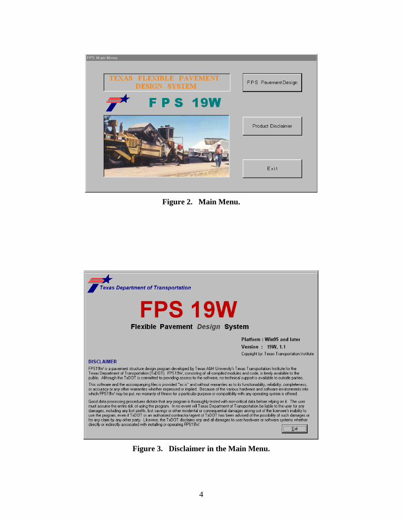
The Main Menu screen (Figure 2) will be displayed for all subsequent runs of FPS 19W.

The options available are:

• “FPS Pavement Design” C This option permits the user to proceed into the

design program. This is normal operation.

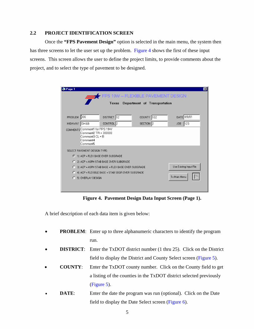
• “Product Disclaimer” C Review the disclaimer statement as shown in Figure 3.

• “Exit” C Exit the program.

4

Figure 2. Main Menu.

Figure 3. Disclaimer in the Main Menu.

5

2.2 PROJECT IDENTIFICATION SCREEN

Once the “FPS Pavement Design” option is selected in the main menu, the system then

has three screens to let the user set up the problem. Figure 4 shows the first of these input

screens. This screen allows the user to define the project limits, to provide comments about the

project, and to select the type of pavement to be designed.

Figure 4. Pavement Design Data Input Screen (Page 1).

A brief description of each data item is given below:

• PROBLEM: Enter up to three alphanumeric characters to identify the program

run.

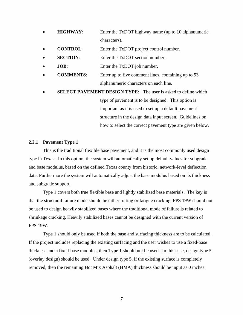
• DISTRICT: Enter the TxDOT district number (1 thru 25). Click on the District

field to display the District and County Select screen (Figure 5).

• COUNTY: Enter the TxDOT county number. Click on the County field to get

a listing of the counties in the TxDOT district selected previously

(Figure 5).

• DATE: Enter the date the program was run (optional). Click on the Date

field to display the Date Select screen (Figure 6).

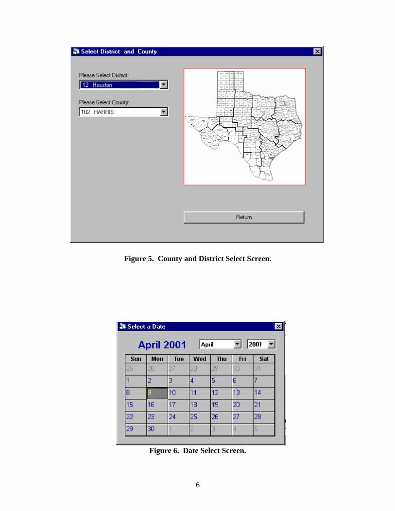
6

Figure 5. County and District Select Screen.

Figure 6. Date Select Screen.

7

• HIGHWAY: Enter the TxDOT highway name (up to 10 alphanumeric

characters).

• CONTROL: Enter the TxDOT project control number.

• SECTION: Enter the TxDOT section number.

• JOB: Enter the TxDOT job number.

• COMMENTS: Enter up to five comment lines, containing up to 53

alphanumeric characters on each line.

• SELECT PAVEMENT DESIGN TYPE: The user is asked to define which

type of pavement is to be designed. This option is

important as it is used to set up a default pavement

structure in the design data input screen. Guidelines on

how to select the correct pavement type are given below.

2.2.1 Pavement Type 1

This is the traditional flexible base pavement, and it is the most commonly used design

type in Texas. In this option, the system will automatically set up default values for subgrade

and base modulus, based on the defined Texas county from historic, network-level deflection

data. Furthermore the system will automatically adjust the base modulus based on its thickness

and subgrade support.

Type 1 covers both true flexible base and lightly stabilized base materials. The key is

that the structural failure mode should be either rutting or fatigue cracking. FPS 19W should not

be used to design heavily stabilized bases where the traditional mode of failure is related to

shrinkage cracking. Heavily stabilized bases cannot be designed with the current version of

FPS 19W.

Type 1 should only be used if both the base and surfacing thickness are to be calculated.

If the project includes replacing the existing surfacing and the user wishes to use a fixed-base

thickness and a fixed-base modulus, then Type 1 should not be used. In this case, design type 5

(overlay design) should be used. Under design type 5, if the existing surface is completely

removed, then the remaining Hot Mix Asphalt (HMA) thickness should be input as 0 inches.

8


This design is used primarily in West Texas where the asphalt stabilized base is placed

directly on the prepared subgrade.


This type is similar to type 2, but in this case a subbase layer is used. This layer can be

either a flexible or treated subbase layer. The system supplies default moduli values for each

layer. The flexible subbase is assigned a value three times greater than the subgrade moduli

value.


This design is similar to type 1, but this time a subbase layer is placed beneath the

flexible base layer. The user should be careful when designing pavements with lime-stabilized

subgrade layers. Type 4 should be used if the user considers the treated layer to be permanent.

If the treated layer is primarily to expedite construction, then this option should not be used. In

that case, use pavement type 1. Pavement type 4 is recommended for full-depth reclamation

designs where the existing structure is milled and treated to form a subbase.

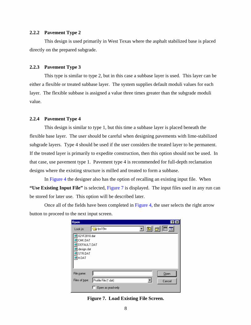
In Figure 4 the designer also has the option of recalling an existing input file. When

“Use Existing Input File” is selected, Figure 7 is displayed. The input files used in any run can

be stored for later use. This option will be described later.

Once all of the fields have been completed in Figure 4, the user selects the right arrow

button to proceed to the next input screen.

Figure 7. Load Existing File Screen.

9

2.3 BASIC DESIGN CRITERIA, PROGRAM CONTROLS, TRAFFIC DATA, AND

ENVIRONMENT AND SUBGRADE INPUTS

The second input data screen displayed is for the basic design criteria input data, the

program control inputs, the traffic data inputs, and the environment and subgrade inputs

(Figure 8). The and keys are for moving forward or backward between the different

input screens.


Each of the data input fields on this screen and on the other input screens have a “Help”

screen associated with them. The “Help” screens give a description of the data item together

with suggested or recommended values. To review the help screen for any field, click on the

field and press the “F1” key. Figure 9 is the help screen for the “Design Confidence Level”

data field. After viewing the help screen, click the “X” button in the top corner to return to the

data input screen. The designer can then input a value or use the value that is displayed.

10

Figure 9. Help Screen for Design Confidence Level.

2.3.1 Basic Design Criteria

A brief description of the basic design criteria inputs is given below:

• Length of analysis period (years) C This period is usually 20 years for

intermediate or major highways and 10 – 15 years for farm-to-market (FM)

highways.

• Minimum time to first overlay (years) C This input defines the length of time

that the initial design must last before placing an overlay. This is a district

option; however, the minimum recommended value is eight years.

• Minimum time between overlays (years) C Eight years is the recommended

minimum value for this input; however, the districts can use a different value.

• Minimum serviceability index C This input pertains to the smoothness of the

pavement surface at the end of the design period. Use 3.0 for all major routes; 2.5

for U.S., state, and FM routes; and 2.0 for low-volume FM routes (average daily

traffic [ADT] < 1000).

• Design confidence level (CL) C This input ranges from level A (80 percent CL)

to level D (99 percent CL). Table 1 provides guidelines on recommended

confidence levels.

11

Table 1. Guidelines on Selecting Confidence Levels.

Confidence

Level

Percentile

Recommended Usage

A

80

Low volume farm-to-market highways < 500 ADT, no major

increase in traffic anticipated

B

90

Intermediate FMs, low volume state highway (SH) and US routes

C

95

Most design work, routes that are anticipated to have

significant growth

D

99 High volume urban interstate highway (IH). This level will

result in substantially thicker initial design thicknesses.

• Interest rate (percentage) C This input is used to discount future expenditures

so that sufficient funds will be available for overlays, maintenance, and salvage

value. Use 7 percent as the interest rate input.

2.3.2 Program Controls

The program control data inputs are described below:

• Number of output pages C The user selects the maximum number of feasible

designs. The system places eight possible designs on each page. By inputting

three (pages) in this field, up to 24 possible designs could be generated.

However, in many cases, fewer than this number is found to be feasible.

• Maximum funds available per square yard for initial construction ($) C This

input should realistically reflect the amount of funds available. A low figure

decreases the number of designs, and the least cost design may be missed. If this

is not a consideration, use 99.

• Maximum total thickness of initial construction C This input should be greater

than the total maximum thickness of all the pavement layers. A smaller than

realistic value for this input can limit the number of designs and can result in a

less than optimal design.

12

• Maximum total thickness of all overlays (inches) C This input is subject to the

geometrics of the pavement cross section. The cost of a 0.5-inch level-up is

always included in the overlay cost, but the 0.5-inch thickness is not to be

included in this data input. Use a realistic value for the maximum overlay

thickness so as not to restrict the design calculations. For most cases, 6 inches is

adequate.

2.3.3 Traffic Data

The FPS 19W traffic data inputs are listed below. These values are provided by TxDOT’s

traffic section in Austin.

• ADT at the beginning of the analysis period (veh/day) C This input is the

average daily traffic at the beginning of analysis period.

• ADT at the end of 20 years (veh/day) C This input is the estimated average

daily traffic at the end of the design period.

• One direction cumulative 18 kip at the end of 20 years C This input is the

number of 18 kip equivalent single axle loads anticipated for the project and is the

most significant design variable. This value is furnished by the Transportation

Planning and Programming Division.

• Average approach speed to the overlay zone (mph) C This input is used to

compute traffic delay costs during overlay operations (values from 55 to 70 mph

are reasonable).

• Average speed through overlay zone (overlay direction) (mph) C This input is

the reduced speed that vehicles must maintain when traveling through the

restricted zone. This input is used in delay cost calculations.

• Average speed through overlay zone (non-overlay direction) (mph) C This

input is the reduced speed (through speed non-overlay direction) that vehicles

must maintain while traveling through the restricted zone.

13

• Percent of ADT arriving each hour of construction C Transportation Planning

and Programming Division can furnish this input based on the time of day that the

construction occurs. For most cases, use 6 percent for rural highways and 5

percent for urban highways.

• Percent trucks in ADT C This input is used to select the appropriate cost and

capacity tables used in the program.

2.3.4 Environment and Subgrade Inputs

The environment and subgrade data inputs are briefly described below.

• District temperature constant C This input is the mean daily temperature above

32°F; it ranges from 16°F in the panhandle districts to 38°F in the Pharr District.

It is used in the traffic equation and represents the susceptibility of the asphalt to

cracking under traffic in cold weather. A value for each TxDOT district has been

calculated and is automatically displayed based on the TxDOT district number

entered previously.

• Swelling probability* C This input should be a fraction between 0 and 1, which

represents the proportion of the project length that is likely to experience

serviceability loss due to swelling clay.

• Potential vertical rise (PVR)* C This input is a measure of how much the

surface of the clay bed can rise if it is supplied with all the moisture it can absorb.

This input value can be estimated for a locale based on the total amount of

differential heave observed or expected to occur over a long period of time or

from the results of a PVR analysis.

• Swelling rate constant* C This input is used to calculate how fast swelling takes

place. Typical input values are between 0.04 for tight soil with good drainage to

0.20 for cracked, open soil with poor drainage, high rainfall, or underground

seeps. *TxDOT recommends that for the first calculation of required thickness that these three values be set to zero to not

consider expansive clay in the initial design. Once the design thickness is calculated, the program should be rerun

with reasonable values in these fields. This procedure will permit the designer to evaluate the loss in pavement life

associated with expansive materials. If this loss is excessive, then an alternate pavement should be considered.

14

As with the previous data input screens, the user should use the mouse to move the cursor

to the field(s) to edit. The designer can return to the previous data input screen by clicking the

left arrow button. When all the data inputs are correct, click the right arrow button to accept the

inputs and to display the next input screen.

2.4 CONSTRUCTION AND MAINTENANCE, DETOUR DESIGN, AND PAVING

MATERIAL DATA

The third and final data input screen is for the construction and maintenance inputs, the

detour design for overlays, and the paving materials (Figure 10).


2.4.1 Construction and Maintenance Data

The construction and maintenance inputs are listed and discussed briefly below.

• Initial serviceability index C This index depends on the materials used and

construction practices. A statewide average of 4.2 for asphaltic concrete

pavements (ACP) is realistic, and surface treatments are 3.8. For a thick ACP, the

initial serviceability can be as high as 4.8.

15

• Serviceability index after overlaying C This input is generally similar to the

serviceability index for initial construction, but the district must input a value

based on their experience. This value cannot be less than the minimum

serviceability index. For most overlays, a value of 4.0 is recommended.

• Minimum overlay thickness C A 0.5-inch level-up is automatically added to this

thickness and is included in the overlay costs. Normal values are 1.5 or 2.0

inches.

• Overlay construction time (hrs/day) C This input represents the expected

number of hours per day that overlay operations take place. It is used in

calculating the number of vehicles that will be delayed by the overlay operation,

which affects traffic delay costs.

• Asphalt compaction density (tons/cy) C This input is used in the delay cost

calculation. A value of 1.9 is recommended.

• Asphalt concrete production rate (tons/hr) C This input is used to calculate the

time it will take to place an overlay and to determine the number of vehicles

delayed by the overlay operation, which affects traffic delay costs.

• Width of each lane (ft) C This input is used to calculate the rate of overlaying

and affects the number of vehicles that are slowed or delayed due to the overlay

work.

• First-year cost of routine maintenance (dollars/lane mile) C The average cost

of routine maintenance for the first year after initial or overlay construction is

represented by this input. A statewide average value is $100 per lane mile.

• Annual incremental increase in maintenance cost (dollars/lane mile) C The

annual incremental increase in routine maintenance cost during each year after

initial or overlay construction is assumed to increase at a uniform rate. This cost

varies from $10 to $100 per lane mile.

16

2.4.2 Detour Design Data

The detour design inputs are included on this input screen and are listed below.

• Detour model used during overlaying C There are five different methods of

handling traffic during overlay operations. The first two methods are for two-lane

roads (with and without shoulders), and the three remaining methods are for four

or more lane roadways. The user should insert the number of the method that will

be used for handling traffic during overlay operations. This value is important as

using the wrong model can generate excessive delay costs and severely impact the

selected design.

• Total number of lanes of the facility C This input is for main lanes only and is

used in determining traffic delay costs during overlay operations.

• Number of lanes open in the overlay direction C This input depends on the

method of handling traffic during overlaying and the number of lanes of the

highway.

• Number of lanes open in the non-overlay direction C This input depends on

the method of handling traffic during overlaying and the number of lanes of the

highway.

• Distance traffic is slowed (overlay direction)(miles) C This input is used in

calculating the time that vehicles are delayed due to overlaying operations and is

input in miles.

• Distance traffic is slowed (non-overlay direction)(miles) C This input is used

in calculating the time that vehicles are delayed due to overlaying operations and

is input in miles.

• Detour distance around the overlay zone (miles) C This input is only valid for

traffic handling method five. Leave this input set at zero unless traffic handling

method five is to be used, in which case the input is the distance in miles that the

traffic is detoured around the overlay zone.

17

2.4.3 Paving Material Data

The available materials, their corresponding layer, moduli, and a reasonable range of

acceptable thicknesses are input in this screen. FPS 19W will look within these ranges to

determine if a design to meet the traffic loading and environmental conditions is possible. If the

constraints are too binding, then a “No Feasible Design” message will be generated.

The default values initially shown in these fields are based on the pavement type selected

in Figure 4. The subgrade modulus is assigned based on the county number. Default subgrade

moduli ranging from 4 ksi (very bad) to 20 ksi (excellent) have been assigned for each Texas

county. In all cases, the user is expected to change these default values with project-specific

values computed using the MODULUS backcalculation system.

Further discussion of each field is provided below:

• Layer designation number C Each construction material that is input into the

program must be accompanied by a unique layer designation number that

indicates the layer in which the material will be used. Each material is also

assigned a unique letter code so that the material can be identified in the output

summary table. The layer numbering is done in sequence from top to bottom.

Surface materials are 1, base materials are 2, etc. The subgrade should be

numbered as the last layer (3 for three-layer design, 4 for four-layer design, etc.).

• Letter code of material C A unique letter code is assigned to each material that

is input (including the subgrade) so that the material can be identified in the

output summary table.

• Name of material C Use the space provided to describe the material in each

layer. The designer can overwrite these names. For example, if a lime-treated

base is used, then the flexible base title should be overwritten.

• In-place cost/completed cubic yard (cy) ($) C The in-place cost of materials

determines the cost of initial construction, cost of overlay construction, and

salvage return. A change in the cost of any material may result in a different

optimal design for that combination. This is a district-specific field.

• Elastic modulus of the material (ksi) C This is a very important variable. The

MODULUS backcalculation program should be used to determine district-

18

specific modulus values of materials in existing pavements from FWD. The new

Windows version of MODULUS is described in the companion Report 0-1869-2

(3). For new pavements to be constructed on new right of ways, the most

important required input is the subgrade modulus value. In this case, the designer

has the following three options to determine a reasonable value for the subgrade

modulus:

Accept the default county-specific values provided within FPS 19W; in

most cases, these values have been shown to be reasonable.

Test an adjacent highway with a similar structure with the FWD, and

backcalculate a subgrade modulus. It is important to ensure that the

pavement sections will be similar. It is not possible to take a subgrade

value backcalculated from a very stiff major highway and use that value to

design a connecting FM route.

Use an approved alternate procedure such as a dynamic cone

penetrometer, or obtain materials for laboratory testing. The Flexible

Pavement Design Section in Austin should be contacted for this

alternative.

Based on analysis of FWD data from around the state, the following values are

considered reasonable for Texas materials. Districts are encouraged to generate their own

moduli values from in-service pavements.

• Asphalt Concrete (AC) Material C This modulus value must be normalized to

the design temperature of 77°F. To conduct this temperature correction, the user

must have the AC temperature recorded at the time the FWD data are collected.

Standard temperature correction procedures are available from TxDOT. For most

surfacing mixes, a value of 500 ksi has been found to be reasonable.

• Asphalt Treated Bases C This value must be temperature corrected to 77°F.

From FWD analysis, typical moduli found on Texas materials for plant-mixed

materials have been measured to range from 300 to 700 ksi. For initial design

purposes, a value of 400 ksi is recommended.

19

• Flexible Base Materials C This step is perhaps the most difficult part of the

design process. For pavement type 1 during the analysis, the program will

automatically adjust the base modulus based on its thickness. For thick flexible

bases, the program may break the base into two different layers with the upper

base having a higher modulus than the lower base. A discussion of this approach

can be found in the appendix of Report 0-1987-2 (1). For pavement type 1

designs, the input modulus value is intended to represent the value that would be

obtained on a 10-inch thick base. If a district is backcalculating a value for a

thick base (greater that 14 inches), then the Design Division in Austin should be

contacted to adjust this value to that anticipated for a 10-inch thick layer.

In pavement type 1, the initial default base value will be based on the

input subgrade modulus. If the user changes the subgrade modulus, then the

default base modulus will also change. For pavement type 1, the user is

encouraged to use the default base modulus. The user can input a new base

modulus but must exercise care. If the same base material is being used around

the district with widely different subgrade support conditions, then it will not be

reasonable to specify the same base modulus independent of subgrade support. A

base with a modulus of 60 ksi on a good subgrade will not have the same modulus

if it is placed directly on a poor subgrade; the good subgrade will confine to the

base, and it is well known that a flexible base has a higher modulus value when it

is confined.

With good support conditions or when the base is placed on a stabilized

subbase, the following moduli values are thought appropriate for Texas base

materials:

Grade 2 Flexible Base 50 ksi

Grade 1 Flexible Base 70 ksi

Lime Stability Material (Grade 2) 50–100 ksi (depends on percent lime)

Lime Fly Ash (FA) Bases 50–100 ksi (depends on percent FA)

Cement Stabilized Materials 80–150 ksi (appropriate for low cement

contents only. FPS 19W does not handle

heavily stabilized bases.)

20

Note that these values have been provided as guidelines. Each district

should generate its own values based on its own materials. Special attention

should be given to flexible bases placed directly on top of stiff subgrade layers.

In these cases, high moduli values can be anticipated for the flexible base layer;

values in excess of 100 ksi have been found when Class 1 materials are placed

over stabilized subbases.

• Subbase materials C These materials are important particularly for pavement

type 4. The most common case is lime-stabilized subgrades. In general, lime-

stabilized subgrades should not be considered in the thickness design

computation. The concern is that the lime layer may not be permanent and that its

strength may disappear after several years in service. In this case, pavement

design 4 should not be used; the design should use pavement type 1. However,

several districts have reported that with high lime levels, the lime layers can be

considered a permanent structural layer. In these cases, a stabilized subgrade

modulus in the range of 30 to 40 ksi are often used.

With full depth reclamation, it is now common to stabilize the existing

structure to form a stiff subbase layer. In these cases, stabilized subgrade values

in the range of 100 to 150 ksi have been measured. It is also feasible to use a

higher flexible base modulus for layers placed directly on top of the stabilized

layer. District experience will dictate the values to use in this case.

• Minimum depth (inches) C The minimum thickness should be carefully selected

to prevent thicknesses that are impractical to construct.

• Maximum depth (inches) C The minimum and maximum layer inputs determine

the range of thicknesses to be considered for each material. The maximum

thickness should be carefully selected to prevent thicknesses that are impractical

to construct. Wide ranges of thicknesses will cause longer computation time. If

the final surfacing is fixed, then the minimum and maximum values should be set

to the same value. If the final surfacing is to be a one- or two-course surface

treatment, then a value of zero should be placed in these fields.

The subgrade thickness field should contain the depth to a stiff layer used

in the MODULUS backcalculation analysis.

21

If the designer wishes to simply check if a selected design is adequate, the

minimum and maximum values can be set to the selected values for each layer.

The program will then check to see if the selected structure will meet the design

requirements.

• Material’s salvage value as percent of original cost C For salvage purposes,

estimate the value of each material at the end of the analysis period and convert

this value to a percent of its original construction value. For example, a granular

base may retain 80 percent of its originally invested value, while only 30 percent

of the value of asphaltic concrete may be usable at the end of the analysis period.

The present worth of the salvaged materials is used in comparing total costs of

alternate designs. It should be remembered that this value has been discounted

for the entire length of the analysis period. It may be a negative value.

• Poisson’s ratio of the material C This input is used in the structural analysis of

each design. These values are normally constant; appropriate values can be found

in the help screens.

• Check C This input checks the number of materials for a given problem. A

number 1 must be input for all materials except for the subgrade material, which

must have a zero input in this field.

This section completes the inputs for a single problem for the FPS 19W program. Click

the left arrow button to go back to previous input screens, and click on the data field(s) to change

input values. When the designer is satisfied with the data inputs, click the “Go” button on the

Pavement Design data input screen (Figure 10) to run the FPS 19W design program. A window

will open to display the “Program Running” message while the FPS 19W program is running

the current problem (Figure 11).

Figure 11. Program Running.

22

2.5 SCREEN DISPLAY OF BEST STRATEGIES

After the FPS 19W program has calculated and ranked the designs, a summary of the best

design strategies in the order of increasing total cost is displayed on the screen (Figure 12). The

number of feasible designs displayed will depend on the number of output pages specified in

Figure 8; there will be a maximum of six designs per page. However, in many cases there may

be only one or two feasible designs.

Figure 12. FPS 19W Result Main Screen.

The summary output shown in Figure 12 includes the total cost, the number of layers, the

thicknesses of the layers, the number of performance periods, the performance period times (in

years), the overlay policy, and the swelling clay loss of serviceability. Click the “Previous

Page” and “Next Page” buttons to view all the design strategies in reverse or forward order. If

there are no feasible designs for the data input, the message shown in Figure 13 will be

displayed. In this case, the input conditions are too restrictive to arrive at a feasible solution.

The designer generally needs to increase the maximum thicknesses of layers, change material

types, or reduce the time to first overlay.

23

Figure 13. No Feasible Design.

Figure 12 is one of the main output screens from FPS 19W. The top area in the screen

contains the project identification information. The next row of buttons provides the designer

with flexibility in reviewing the results. The “Previous Page” and “Next Page” buttons will

allow the designer to view the alternative feasible pavement designs if more than one page of

results is available. The remaining options are described in the following sections.

2.5.1 Print/Save the File

Click the “Print/Save File” button to view the complete output of the current FPS 19W

problem. The “View FPS Results” screen (Figure 14) shows the output of the current FPS 19W

problem in a format similar to that provided in earlier DOS versions of FPS 19. Click the “Print

File” button to obtain a hard copy print-out. The input data for the current problem and the full

output for the current problem can be saved by clicking the “Save to File” button. Figure 15

shows the window the with folder, filename, file type, and file attribute to be specified to save

the current input data file or the current output data file. The current FPS 19W data output is

always saved in the “FPS 19W.OUT” file in the root directory unless the user has specified a

particular name for saving the FPS 19W output.

24

Figure 14. View FPS 19W Result File Screen.

Figure 15. Save FPS 19W Data File and Result File.

25

2.5.2 Re-Run FPS

Click the “Re-Run FPS” button to return control to the input screen shown in Figure 8

while retaining the previously input values. The FPS 19W program can be re-run with the same

data input values, or the data input values can be edited, and the problem should be re-run as

desired. An entirely new problem should be run by clicking the “Return to Main Menu”

button.

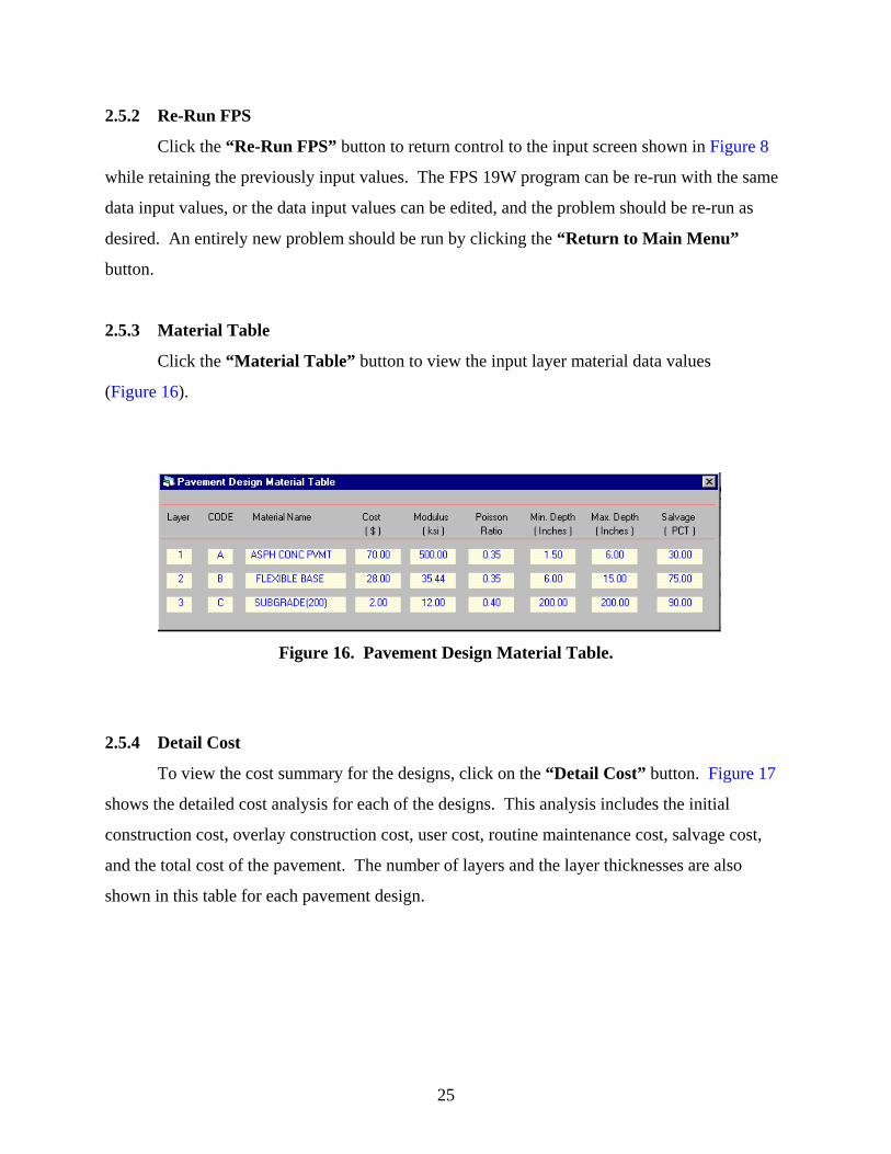
2.5.3 Material Table

Click the “Material Table” button to view the input layer material data values

(Figure 16).

Figure 16. Pavement Design Material Table.

2.5.4 Detail Cost

To view the cost summary for the designs, click on the “Detail Cost” button. Figure 17

shows the detailed cost analysis for each of the designs. This analysis includes the initial

construction cost, overlay construction cost, user cost, routine maintenance cost, salvage cost,

and the total cost of the pavement. The number of layers and the layer thicknesses are also

shown in this table for each pavement design.

26

Figure 17. Pavement Design Cost Analysis Screen.

2.6 CHECKING THE FPS 19W DESIGNS

It is TxDOT policy that the designs generated by FPS 19W should be checked with an

alternative design procedure. This procedure is described in this section. The designer must first

review the feasible designs shown in Figure 12 and select one for detailed review. The feasible

designs are ranked in terms of lowest total cost. The next step in the analysis is to proceed to the

design check phase. For the selected pavement design, click the “Check Design” button at the

bottom of the design. Figure 18 will then be displayed, showing the selected design and the

options available. These include:

• Print Produces a hard copy of the select design, which should be

included in the standard TxDOT design report.

• Previous Design Displays the next lower cost feasible design.

• Next Design Displays the next higher cost feasible design.

• All Design Shows all of the designs available (six per page), as shown

in Figure 19.

• Design Check Lets the designer check the structural adequacy of the FPS

19W design by running alternate design programs to check

the pavement structure. This option is shown in Figure 20,

and it will be described later in this section.

• Stress Analysis Permits the user to calculate stress/strains and deflections

for the selected pavement design. This option will be

described later in this section.

27

Figure 18. One Design Check Menu.

Figure 19. All Design Plots Screen.

28

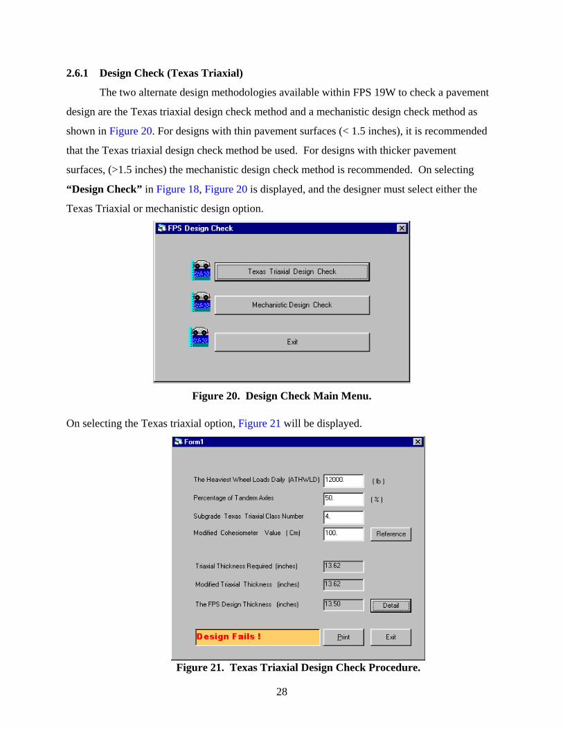
2.6.1 Design Check (Texas Triaxial)

The two alternate design methodologies available within FPS 19W to check a pavement

design are the Texas triaxial design check method and a mechanistic design check method as

shown in Figure 20. For designs with thin pavement surfaces (< 1.5 inches), it is recommended

that the Texas triaxial design check method be used. For designs with thicker pavement

surfaces, (>1.5 inches) the mechanistic design check method is recommended. On selecting

“Design Check” in Figure 18, Figure 20 is displayed, and the designer must select either the

Texas Triaxial or mechanistic design option.

Figure 20. Design Check Main Menu.

On selecting the Texas triaxial option, Figure 21 will be displayed.

Figure 21. Texas Triaxial Design Check Procedure.

29

In Figure 21, the designer must provide input to the top four boxes; the results of the analysis

are shown in the lower three boxes. Details of the Texas triaxial procedure can be found in the

standard TxDOT design manual (4). The required inputs for this option are as follows:

• Average of Ten Heaviest Wheel Loads (ATHWLD) C This input is the average

of the 10 heaviest wheel loads that the pavement is anticipated to carry. It is a

standard traffic statistic generated in the traffic report from Austin.

• Percentage Tandum Axles C This input is the percent of tandum axles from a

traffic report.

• Subgrade Texas Triaxial Class C The subgrade Texas triaxial class (TTC)

number is a soil strength number generated by running TxDOT standard test

117-E. Values range from 3.0 (sandy/gravel subgrade) to 6.5 (extremely weak)

plastic soils. In practice, the standard test is rarely run. Most districts have

reports showing the TTC for standard soils in their area. Other districts have

generated their own approaches to obtaining TTC. Some use calibrations to other

standard tests, such as plasticity index, while others are starting to develop

correlations to dynamic cone results. This is a district-specific input.

• Modified Cohesiometer Value C The Texas triaxial procedure is based on

computing a depth of cover of better material to protect the subgrade for shear

failure. In the preliminary analysis, the better material is assumed to be higher

quality flexible base. However, several districts use treated bases. To account for

the improved load spreading capabilities of treated bases, a thickness reduction

factor is introduced. This process involves assigning a cohesiometer value for

each treated base and using this value to compute an appropriate thickness

reduction factor. To view the approved cohesiometer values, the user should

select the “Reference” button. Figure 22 will then be displayed. To select any

value from within this table, place the cursor over the text, and double click with

the left mouse button. The selected value will be returned to Figure 21.

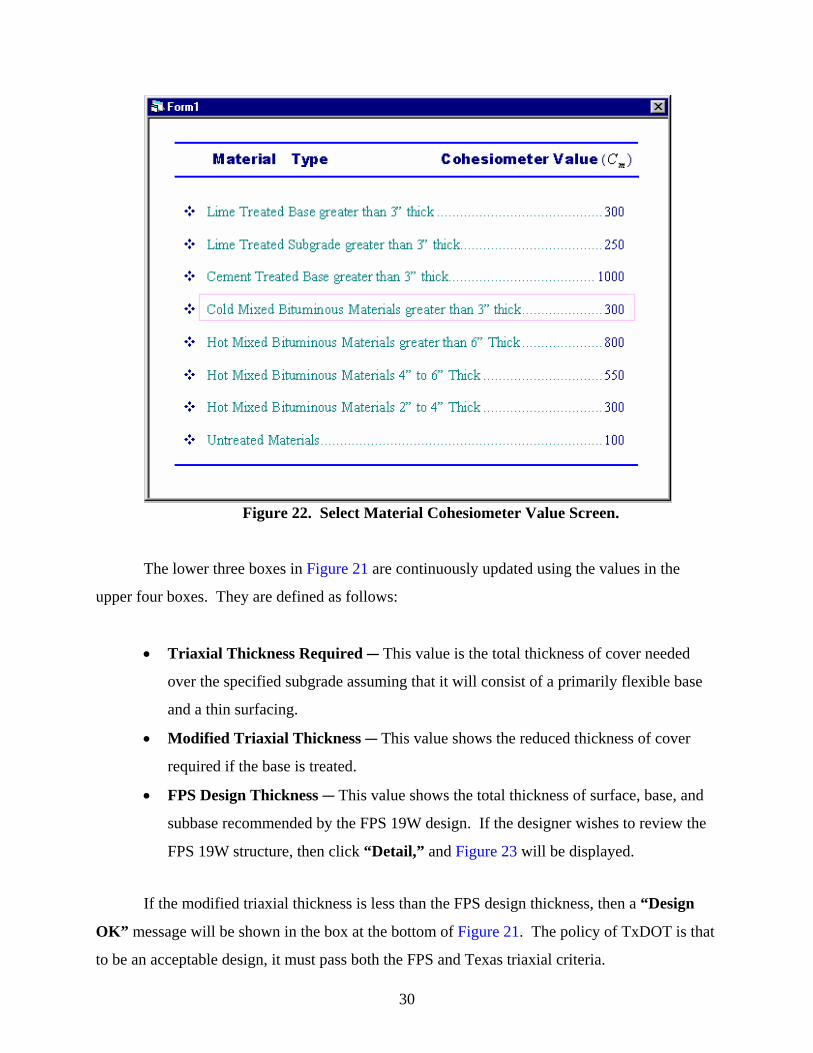
30

Figure 22. Select Material Cohesiometer Value Screen.

The lower three boxes in Figure 21 are continuously updated using the values in the

upper four boxes. They are defined as follows:

• Triaxial Thickness Required C This value is the total thickness of cover needed

over the specified subgrade assuming that it will consist of a primarily flexible base

and a thin surfacing.

• Modified Triaxial Thickness C This value shows the reduced thickness of cover

required if the base is treated.

• FPS Design Thickness C This value shows the total thickness of surface, base, and

subbase recommended by the FPS 19W design. If the designer wishes to review the

FPS 19W structure, then click “Detail,” and Figure 23 will be displayed.

If the modified triaxial thickness is less than the FPS design thickness, then a “Design

OK” message will be shown in the box at the bottom of Figure 21. The policy of TxDOT is that

to be an acceptable design, it must pass both the FPS and Texas triaxial criteria.

31

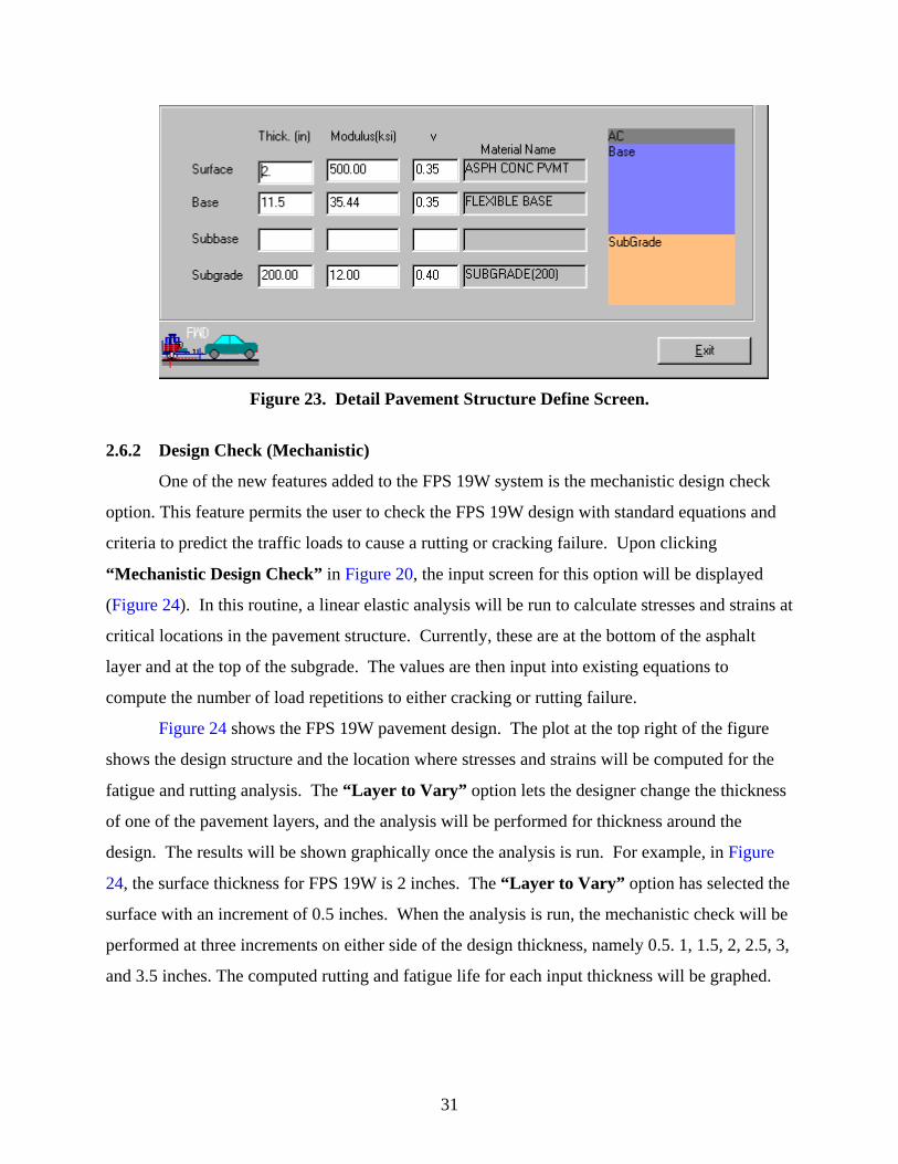
Figure 23. Detail Pavement Structure Define Screen.

2.6.2 Design Check (Mechanistic)

One of the new features added to the FPS 19W system is the mechanistic design check

option. This feature permits the user to check the FPS 19W design with standard equations and

criteria to predict the traffic loads to cause a rutting or cracking failure. Upon clicking

“Mechanistic Design Check” in Figure 20, the input screen for this option will be displayed

(Figure 24). In this routine, a linear elastic analysis will be run to calculate stresses and strains at

critical locations in the pavement structure. Currently, these are at the bottom of the asphalt

layer and at the top of the subgrade. The values are then input into existing equations to

compute the number of load repetitions to either cracking or rutting failure.

Figure 24 shows the FPS 19W pavement design. The plot at the top right of the figure

shows the design structure and the location where stresses and strains will be computed for the

fatigue and rutting analysis. The “Layer to Vary” option lets the designer change the thickness

of one of the pavement layers, and the analysis will be performed for thickness around the

design. The results will be shown graphically once the analysis is run. For example, in Figure

24, the surface thickness for FPS 19W is 2 inches. The “Layer to Vary” option has selected the

surface with an increment of 0.5 inches. When the analysis is run, the mechanistic check will be

performed at three increments on either side of the design thickness, namely 0.5. 1, 1.5, 2, 2.5, 3,

and 3.5 inches. The computed rutting and fatigue life for each input thickness will be graphed.

32

Figure 24. Mechanistic Design Check Main Screen.

The bottom part of Figure 24 permits the user to select which rutting and cracking criteria

to use in the life prediction. The default values are those proposed by the Asphalt Institute. The

program has a range of possible criteria available. Clicking the fatigue equation box will display

Figure 25. This screen shows a range of published criteria from various agencies (5). If the

designer wants to use one of these criteria, then place the cursor over the required equation and

double click with the left mouse button. Control will return to Figure 24, and new values will

appear in the f1, f2, and f3 boxes. A similar option is provided for the rutting analysis in Figure

26.

33

Figure 25. Select Fatigue Cracking Model Screen.

Figure 26. Select Subgrade Strain Criteria Screen (Rutting Analysis).

Click the “Run” button (Figure 24) to perform the fatigue and rutting analysis using the

fatigue and rutting models selected previously. Figure 27 shows the results of the mechanistic

design check for the pavement design. Plots of the crack life and rutting life are shown on the

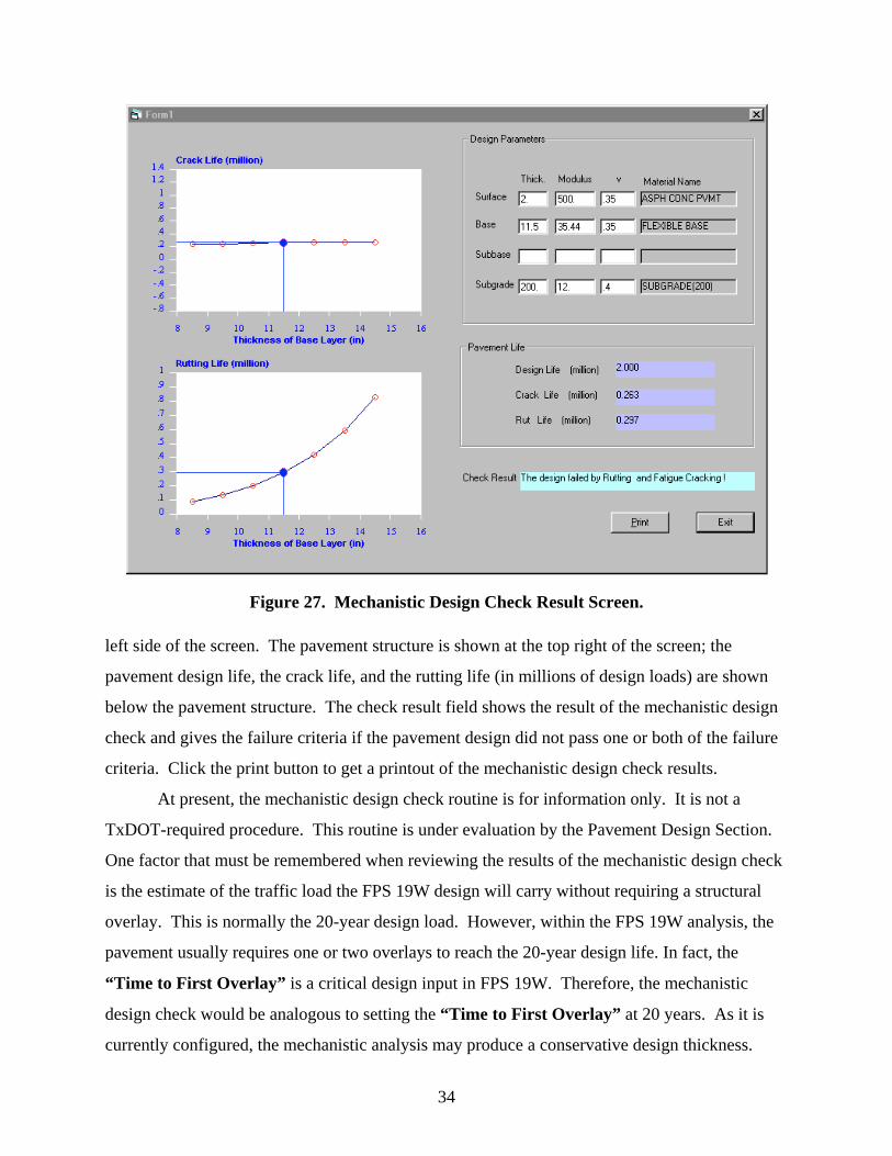
34

Figure 27. Mechanistic Design Check Result Screen.

left side of the screen. The pavement structure is shown at the top right of the screen; the

pavement design life, the crack life, and the rutting life (in millions of design loads) are shown

below the pavement structure. The check result field shows the result of the mechanistic design

check and gives the failure criteria if the pavement design did not pass one or both of the failure

criteria. Click the print button to get a printout of the mechanistic design check results.

At present, the mechanistic design check routine is for information only. It is not a

TxDOT-required procedure. This routine is under evaluation by the Pavement Design Section.

One factor that must be remembered when reviewing the results of the mechanistic design check

is the estimate of the traffic load the FPS 19W design will carry without requiring a structural

overlay. This is normally the 20-year design load. However, within the FPS 19W analysis, the

pavement usually requires one or two overlays to reach the 20-year design life. In fact, the

“Time to First Overlay” is a critical design input in FPS 19W. Therefore, the mechanistic

design check would be analogous to setting the “Time to First Overlay” at 20 years. As it is

currently configured, the mechanistic analysis may produce a conservative design thickness.

35

2.7 STRESS ANALYSIS

Click the “Stress Analysis” button on the “Check One Design” menu (Figure 18) to

perform a stress analysis for the pavement design. The “Stress Analysis is Running” screen

will be displayed while the stress analysis program is running. The results of the stress analysis

for the pavement design are displayed in the “Stress and Strain Analysis” screen (Figure 28).

The WESLEA® five-layer isotropic system program developed by the USAE Waterways

Experiment Station is the program used for the stress and strain analysis (6). Click the “Print

Results” button for a printout of the stress analysis results, or click the “Exit” button to return to

the Check Designs menu screen.

A

B C

D

E

F

Figure 28. Stress and Strain Analysis Screen.

36

Each of the marked areas include the following information:

A Permits the user to change the load, load configuration, and pavement layer information.

B Shows the x and y locations and the layer in which the stress analysis will be performed.

C Shows numeric results from the stress analysis–this is for the folder open in the E window.

D Permits the designer to change the location where the computations are to be made to other

default locations–these could be either vertically or horizontally throughout the structure.

Using the “Other” label, it is possible to move the measurement points to the surface of the

pavement to simulate Falling Weight Deflectometer sensor locations.

E A series of folders containing the results of the stress analysis–by selecting a different folder,

a new set of results will be displayed graphically. These will be described later.

F Graphically shows the pavement structure and the locations where the calculations will

be made.

The options in each of these areas will now be discussed. The designer may wish to

change the loading configuration or locations of stress/strain computation. Once any change is

made, select the “Run Analysis” button to update the computed values.

To change the load configuration (Part A), click on the “Load” tab (Figure 29) to

change the load type, tire pressure, load radius, or the tire spacing. Click the “Pavement

Structure” tab (Figure 30) to change the layer thickness, layer modulus value, or the layer with

Poisson=s Ratio of any or all of the pavement layers for a new analysis. Click the “Unit System”

tab (Figure 31) to select the units for the analysis.

Figure 29. Define the Load and Load Axle Configuration.

37

Figure 30. Pavement Structure Data.

Figure 31. Unit System Selection.

Part B of Figure 28 allows for the specification of the location of the 10 points at which

the stress and strain analysis will be performed. Move the cursor to the appropriate field to

indicate the layer, the horizontal distance (x) from the load, and the depth beneath the surface (2)

at which to perform the analysis (Figure 32). Note the color labels shown in Figure 32 are also

shown graphically in F. When a change is made to any location, that button will also move on

the graph. It is also possible to use the mouse to change the location of any button in F, and this

will automatically be changed in Figure 32.

38

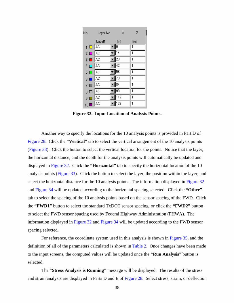
Figure 32. Input Location of Analysis Points.

Another way to specify the locations for the 10 analysis points is provided in Part D of

Figure 28. Click the “Vertical” tab to select the vertical arrangement of the 10 analysis points

(Figure 33). Click the button to select the vertical location for the points. Notice that the layer,

the horizontal distance, and the depth for the analysis points will automatically be updated and

displayed in Figure 32. Click the “Horizontal” tab to specify the horizontal location of the 10

analysis points (Figure 33). Click the button to select the layer, the position within the layer, and

select the horizontal distance for the 10 analysis points. The information displayed in Figure 32

and Figure 34 will be updated according to the horizontal spacing selected. Click the “Other”

tab to select the spacing of the 10 analysis points based on the sensor spacing of the FWD. Click

the “FWD1” button to select the standard TxDOT sensor spacing, or click the “FWD2” button

to select the FWD sensor spacing used by Federal Highway Administration (FHWA). The

information displayed in Figure 32 and Figure 34 will be updated according to the FWD sensor

spacing selected.

For reference, the coordinate system used in this analysis is shown in Figure 35, and the

definition of all of the parameters calculated is shown in Table 2. Once changes have been made

to the input screens, the computed values will be updated once the “Run Analysis” button is

selected.

The “Stress Analysis is Running” message will be displayed. The results of the stress

and strain analysis are displayed in Parts D and E of Figure 28. Select stress, strain, or deflection

39

(Figure 36) for the 10 analysis points to be displayed in tabular form. Note that the stress, strain,

or deflection selected is automatically displayed in graphical form (Figure 37). Click on the

appropriate tab in Figure 37 to display the stress, strain, or deflection in graphical form, and the

display in Figure 36 will be automatically updated. Click the “Print Result” button to get a

printout of the stress and strain analysis (Figure 36), or click the “Exit” button to return to the

“Check One Design” menu.

The stress analysis routine is optional at the present time. It has been included to permit

TxDOT design engineers to become more familiar with the mechanistic design principles. One

practical application of the stress analysis routine could be to use the FWD option and to use the

system to predict the ideal deflection basin for the as-designed pavement. The designer could

then use these “ideal” values to check the resulting pavement design with an FWD after

construction.

Figure 33. Define the Location of the Analysis Points.

40

Figure 34. Mouse Locates the Analysis Points.

Figure 35. The Coordinate System Used in the Stress Analysis.

Y

X

Z

X0

AC

Base

Subgrade

Rock

Tire Spacing Tire Load

41

Figure 36. Stress and Strain Analysis Result Table.

Figure 37. Stress and Strain Analysis Result Charts.

42

Table 2. Definition of All the Stress and Strains Computed in Stress Analysis.

Displacement in three directions x, y, z

Ux ................................................Displacement in x direction

Uy ................................................Displacement in y direction

Uz ................................................Displacement in z direction

Stress

Sx..............................σx Stress in x direction

Sy..............................σy Stress in y direction

Sz ..............................σz Stress in z direction

S1..............................σ1 1st principal stress

S2..............................σ2 2nd principal stress

S3..............................σ3 3rd principal stress

Shear Stress

Tyz............................τyz Shear stress in yz plan

Txz............................τxz Shear stress in xz plan

Txy............................τxy Shear stress in xy plan

Strain

Ex..............................εx Strain in x direction

Ey..............................εy Strain in y direction

Ez..............................εz Strain in z direction

EPS1 .........................ε1 1st principal strain

EPS2 .........................ε2 2nd principal strain

EPS3 .........................ε3 3rd principal strain

43

REFERENCES

1. Scullion, T., and Michalak, C., “Flexible Pavement Design System (FPS) 19W: User’s

Manual,” Research Report 1987-2, Texas Transportation Institute, Texas A&M

University, College Station, Texas, 1997.

2. Michalak, C. H., and Scullion T., “Modulus 5.0: User’s Manual,” Research Report

1987-1, Texas Transportation Institute, Texas A&M University, College Station, Texas,

1995.

3. Liu, W., and Scullion, T., “Modulus 6.0 for Windows: User’s Manual,” Research Report

0-1869-2, Texas Transportation Institute, Texas A&M University, College Station,

Texas, 2001.

4. “Flexible Pavement Designers Manual, Part I,” Texas State Department of Highway and

Public Transportation, Highway Design Division, 1972.

5. Huang, Y. H., “Pavement Analysis and Designs,” Prentice Hall, 1993.

6. Van Cauwelaert, F. J., Alexander, D. R., White, T. D., and Barker, W. R., “Multilayer

Elastic Program for Backcalculating Layer Moduli in Pavement Evaluation: In

Nondestructive Testing of Pavements and Backcalculating Moduli,” STP 1026, ASTM,

Philadelphia, Pennsylvania, 1989.

45

APPENDIX

COMPARING FPS 11 AND FPS 19W

In the development of the FPS 19W program, a comparison was made with design

recommendations from the FPS 11 system, which had been in operation in TxDOT since the

mid-1970s. Many TxDOT engineers were comfortable with the designs generated by FPS 11.

However, FPS 11 requires stiffness coefficients that are computed from Dynaflect data, whereas

FPS 19W requires moduli from FWD analysis. With the assistance of TxDOT personnel, moduli

and stiffness coefficient equivalencies were established, and a sensitivity analysis was performed

comparing FPS 11 and FPS 19W. The sensitivity analysis is included in this Appendix.

1) The design thickness produced by FPS 19W and FPS 11 were similar for the pavements

with flexible bases (Pavement Types 1 and 4) if:

a. the reliability levels were adjusted. Reliability level C in FPS 19W appears

equivalent to Level D in FPS 11.

b. the Corps of Engineers procedure for providing increased base modulus based on

increase thickness is used. Following this procedure, the new FPS 19W divides

bases greater than 10 inches into 2 bases, giving the upper base a higher stiffness.

c. the default base modulus generated by the program is used. Overwriting this

value by using a fixed base modulus independent of subgrade support was found

to be non-conservative for low subgrade moduli, especially if a high modulus (for

example 50 ksi) is assumed for a base sitting on a subgrade with modulus less

than 10 ksi. In general, the base to subgrade modulus ratio of 3 appeared

reasonable.

2) For the thick asphalt pavements (pavement types 2 and 3), the trends were similar, but

some differences were found. Again the reliability level of C in FPS 19W appears

equivalent to level D in FPS 11. The biggest difference is in the impact of thickness and

support of the lower layers on the final design. FPS 19W is more conservative than FPS

11 in that the lower layers have less impact on the final design thickness. More work is

required in this area.

46

TECHNICAL MEMORANDUM TEXAS DEPARTMENT OF TRANSPORTATION

Cooperative Research Program TO: Mark McDaniel, TxDOT FROM: Tom Scullion, TTI SUBJECT: Comparing FPS 19W and FPS 11 DATE: April 3, 2000 The attached figures show the results of a comparison of the design life predicted for both FPS 11 and FPS 19W for a range of comparable pavement design scenarios. The rationale for the comparison was the assumption that the trends in the FPS 11 program (not the absolute values) are thought to be reasonable. The design parameter reported in all of the following graphs is the Time to First Overlay. This is the critical input requirement which frequently governs ultimate pavement thickness with either FPS 11 or FPS 19. The major conclusions from this analysis are as follows: 1) For Pavement Type 1 (Thin HMA over flex base), the comparison between FPS 11 and

FPS 19W were reasonable. However it appears that a reliability level of D in FPS 11 is equivalent to a C in FPS 19.

2) For Pavement Type 1 it appears that the current DOS version of FPS 19W does not give as much benefit to thick ( > 10 inches) granular bases as FPS 11. This observation caused a review of the methodology of assigning moduli values within FPS 19W, particularly of breaking bases up into a lower and upper base, with the upper base having a higher moduli value. Updated equations from the US Army Corps of Engineers were adopted for this purpose. These were forwarded to TxDOT in a technical memo dated Sept. 15, 1999. These updated equations have been incorporated into the current Windows version of FPS 19.

3) For Pavement Type 4 ( Thin HMAC, Flex Base , Stabilized subbase, subgrade) the comparison between FPS 11 and 19W were reasonable but they could be improved with the adoption of non-linear material properties where the base and subbase moduli are functions of the subgrade moduli. In the current version of FPS 19W these values are user defined and often fixed by each district based on their experience. A later version of FPS 19W should incorporate this feature.

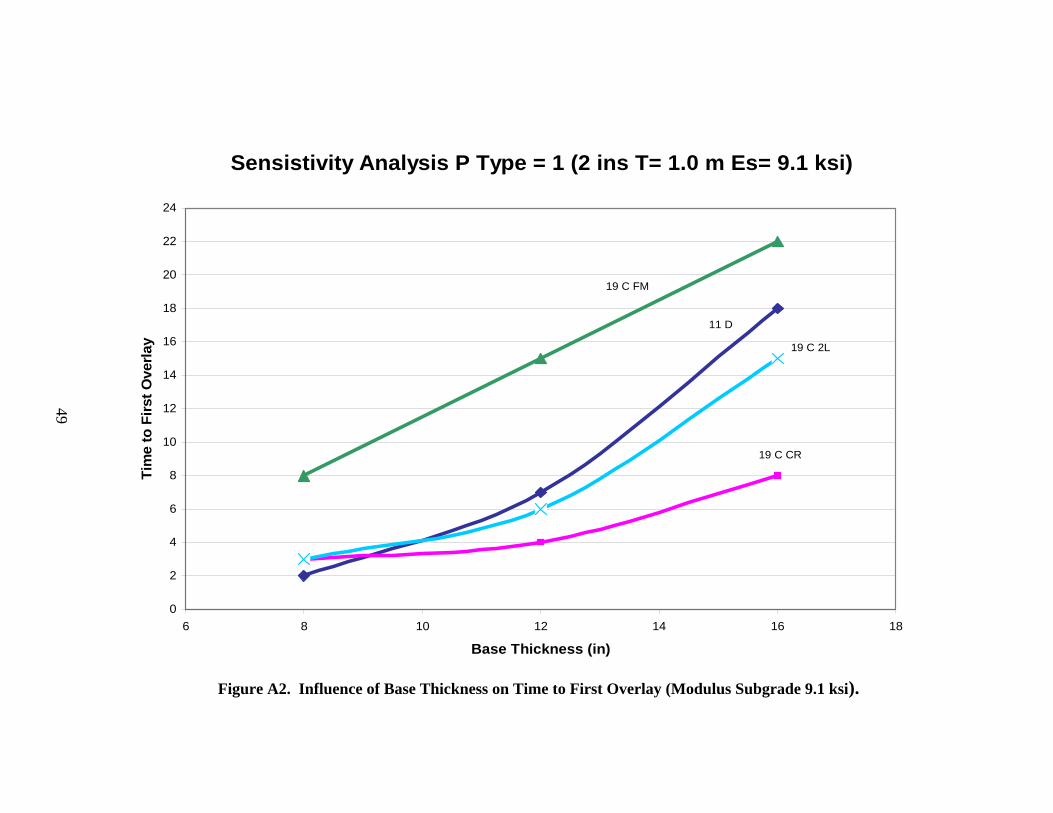
4) With thick Asphalt Stabilized Base (ASB) pavements, the FPS 19W design thicknesses are less dependent on subbase and subgrade moduli. For example in Pavement Design Type 3 the thickness of the ASB is little influenced by the thickness or strength of the flexible subbase layer.

47

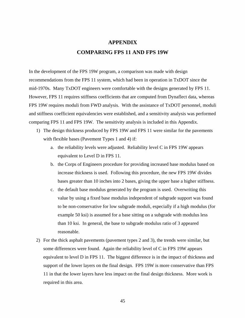
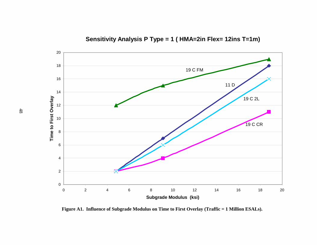
PAVEMENT TYPE 1

A summary of the Sensitivity Analysis results from the FPS11/FPS19W comparison is shown in Figures A1 and A2. This summary is for Pavement Type 1 (Thin HMA, over Flexible Base on subgrade).

NOTE: Because of the differences found between the current DOS version of FPS 19W and FPS 11, substantial changes were made to the method of assigning moduli values within the new FPS 19W (the Windows version). A discussion of the procedure for calculating the modulus of the flexible base is given in another Technical Memorandum (dated Sept 15, 1999) which also contains the complete results from the sensitivity analysis. With thick base layers (>10 inches) both the current DOS FPS 19 and the new WINDOWS version breaks the base into an upper and lower base layer, with the upper base having a higher modulus. The Windows version gives more benefit to thicker bases than the DOS version. The variables used in the current sensitivity analysis are:

Traffic (T) 0.2, 1 and 3 million ESAL’s Thickness of Flexible Base (Flex) 8, 12 and 16 ins Subgrade Modulus (Es) FPS19W (4.8, 9.1, 18.9 ksi), FPS11 (.2, .23, .27) Flex Base Modulus = 60 ksi (fixed) or Calc. using COE Equation Flex Base SC (FPS 11) = 0.55 (fixed) HMA Modulus = 500ksi, SC=0.96, Thickness = 2 inches In the attached graphs the following labels are used,

11 D FPS 11 at reliability level D 19 C CR FPS 19 at reliability level C, current DOS version 19 C 2L FPS 19 at reliability level C, two layers, new Windows version 19 C FM FPS 19 at reliability level C, fixed base modulus of 60 ksi

The following conclusions are drawn from the attached graphs: 1) In both graphs, the FPS 19W results are similar in shape to those obtained with FPS 11; they

appear better than the current FPS 19 DOS results. 2) Reliability level D in FPS 11 is similar to Level C in FPS 19W. 3) Use of fixed base moduli values can be dangerous when used over poor subgrades. Recommendations 1) The new procedure for assigning the flexible base moduli in FPS 19W appears to give

comparable trends to those in FPS 11. 2) Districts should be made aware of the potential problems of always using the same moduli

values for flexible bases.

Sensitivity Analysis P Type = 1 ( HMA=2in Flex= 12ins T=1m)

0

2

4

6

8

10

12

14

16

18

20

0 2 4 6 8 10 12 14 16 18 20

Subgrade Modulus (ksi)

Tim

e to

Firs

t Ove

rlay

19 C FM

11 D

19 C 2L

19 C CR

Figure A1. Influence of Subgrade Modulus on Time to First Overlay (Traffic = 1 Million ESALs).

48

Sensistivity Analysis P Type = 1 (2 ins T= 1.0 m Es= 9.1 ksi)

0

2

4

6

8

10

12

14

16

18

20

22

24

6 8 10 12 14 16 18

Base Thickness (in)

Tim

e to

Firs

t Ove

rlay

19 C FM

11 D

19 C 2L

19 C CR

Figure A2. Influence of Base Thickness on Time to First Overlay (Modulus Subgrade 9.1 ksi).

49

50

PAVEMENT TYPE 2

A summary of the Sensitivity Analysis results from the FPS11/FPS19W comparison is shown in the following 3 graphs (Figures A3-A5). This is for Pavement Type 2 (HMA, ASB on subgrade). NOTE: No changes have been made to the system so the current DOS version of FPS 19 should give identical results to the new Windows version. The variables used in the current sensitivity analysis are:

Traffic 1, 5, 10 million ESAL’s Thickness of ASB 3, 5, 8 ins Subgrade Modulus FPS19 (4.8, 9.1, 18.9 ksi), FPS11 (.2,.23,.27) ASB Modulus = 400ksi, SC=0.92 In general all three graphs show similar trends. The reliability level C seems to be almost equivalent between FPS 11 and FPS 19. The relationship between time to first overlay and ASB thickness and traffic level are similar for both FPS 11 and FPS 19. The major difference between the graphs is that FPS 11 is more sensitive to changes in subgrade modulus. At low moduli values the FPS 11 pavement has shorter life (3 years in FPS11 as opposed to 11 years with FPS19) at high moduli values the FPS 11 pavement lasts longer (29 years as opposed to 20 years with FPS 19). In general the stiffness of the lower layers beneath the thick ASB layer have less influence on pavement life in FPS 19 than FPS 11. This is because FPS 19 uses a linear elastic program to compute the design parameter [Surface Curvature Index (SCI)]. The computed SCI is strongly dependent on the modulus of the upper 12 inches of the pavement and less dependent on the subgrade or subbase modulus. Which one is correct? (Who knows – It may be worth comparing the predictions with those from the Asphalt Institute). This is not a very common design in Texas, and seems to be used only in West Texas on high strength subgrades. One interesting point is that in the middle range (average traffic – average modulus) the two programs give very similar results. The differences at the two extremes (very weak or very strong moduli) are not as significant as found on other pavement types. In reality this may not be a problem as ASB layers are never placed directly over poor subgrades. Weak subgrade layers would be stabilized with lime or cement, or a Pavement Type 3 would be used. Recommendations 1) Use the Asphalt Institute procedure to check the trends in pavement thickness with regard to

changes in subgrade modulus and ASB thickness. 2) At present no major changes are anticipated for this pavement design type.

Sensitivity Analysis P Type=2 ( 2ins, Es= 18.9ksi, T=5m)

0

5

10

15

20

25

30

35

3 4 5 6 7 8 9

ASB thickness (ins)

Tim

e to

Firs

t Ove

rlay

(yea

rs)

11 C

19 C

Figure A3. Influence of ASB Thickness on Time to First Overlay.

51

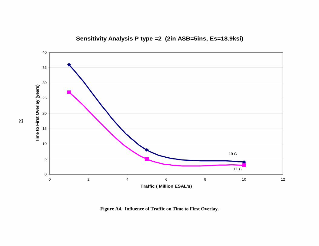
Sensitivity Analysis P type =2 (2in ASB=5ins, Es=18.9ksi)

0

5

10

15

20

25

30

35

40

0 2 4 6 8 10 12

Traffic ( Million ESAL's)

Tim

e to

Firs

t Ove

rlay

(yea

rs)

19 C

11 C

Figure A4. Influence of Traffic on Time to First Overlay.

52

Sensitvity Analysis P.Type=2 (2ins ASB=8ins T=5m)

0

5

10

15

20

25

30

35

4 6 8 10 12 14 16 18 20


Tim

e to

Firs

t Ove

rlay

(yea

rs)

19 C

11 C

Figure A5. Influence of Subgrade Modulus on Time to First Overlay for Pavement Type 2.

53

54

PAVEMENT TYPE 3

A summary of the Sensitivity Analysis results from the FPS11/FPS19W comparison is shown in the following four graphs (Figures A6-A8). This is for Pavement type 3 (HMA, ASB, Flex Base on subgrade). The variables were used in the current sensitivity analysis are: Traffic 2, 8, 14 million ESAL’s Thickness of ASB 4, 8, 12 ins Thickness of Flex base 6, 10, 14 ins Subgrade Modulus FPS19 (4.8, 9.1, 18.9 ksi), FPS11 (.2,.23,.27) ASB Modulus = 400ksi, SC=0.92 Flex base Modulus 3*subgrade modulus or 0.55 in FPS 11 The influence of 18 kip level is similar in both pavement types, and again it appears that reliability level D in FPS 11 is equivalent to level C in FPS 19W. However, the major difference from these results is that the lower layers (flexible base thickness and subgrade modulus) have significantly less impact on the design life in FPS 19W. The thickness of the flex base increase from 6 to 14 inches and the FPS 19W life only increases from 8 to 9 years. A similar change in FPS 11 has a change in life from 5 to 26 years. Recommendations 1) In FPS 19W the thickness of the flexible base beneath the ASB has little impact

on pavement life. For this option TxDOT’s Design Division should recommend a fixed thickness of flex base 6 or 8 inches.

2) The reliability level D in FPS 11 appears equivalent to Level C in FPS 19W.

Sensitivity analysis P Type 3 (2in ASB=8ins Flex=6ins Es=9.1ksi)

0

5

10

15

20

25

30

35

40

45

0 2 4 6 8 10 12 14 16

Traffic (Millions ESAL's)

Tim

e to

Firs

t Ove

rlay

(yea

rs)

11 C

19 C

11 D

Figure A6. Influence of Traffic on Time to First Overlay (Pavement Type 3).

55

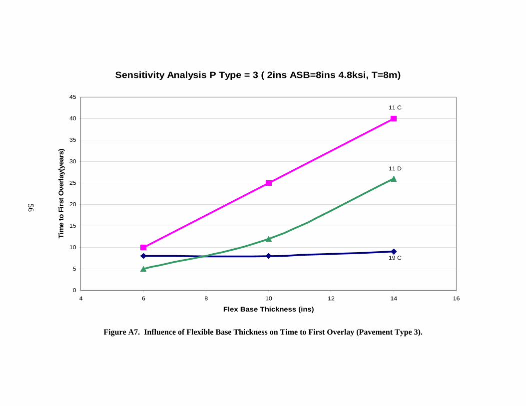
Sensitivity Analysis P Type = 3 ( 2ins ASB=8ins 4.8ksi, T=8m)

0

5

10

15

20

25

30

35

40

45

4 6 8 10 12 14 16

Flex Base Thickness (ins)

Tim

e to

Firs

t Ove

rlay(

year

s)

11 C

11 D

19 C

Figure A7. Influence of Flexible Base Thickness on Time to First Overlay (Pavement Type 3).

56

Sensitivity Analysis PType = 3 ( 2ins, Flex=6ins ASB=8ins T=8m)

0

5

10

15

20

25

30

35

40

45

4 6 8 10 12 14 16 18 20


Tim

e to

Firs

t Ove

rlay

(yea

rs)

11 C

11 D

19 C

Figure A8. Influence of Subgrade Modulus on Time to First Overlay (Pavement Type 3).

57

58

PAVEMENT TYPE 4

A summary of the Sensitivity Analysis results from the FPS11/FPS19W comparison is shown in the following four graphs. This is for Pavement Type 4 (HMA, Flexible base, stabilized subgrade on subgrade). The variables were used in the current sensitivity analysis are: Traffic (T) 1, 5, 10 million ESAL’s Subgrade Modulus (Es) FPS19 (4.8, 9.1, 18.9 ksi),

FPS11 (.2,.23,.27) Stab. Subgrade Modulus (SS) = 35ksi, SC = 0.32

Flex Base Modulus (Flex) = 60ksi, SC=0.55 HMA Surface thicknesses 2ins, 5ins Thickness of Flex base 6, 10, 14 ins Stab. Subgrade (SS) thickness 6ins The attached graphs show, as was the case with Pavement Type = 1, that fixing moduli values, which is common practice for this pavement type, produces results which are significantly different from FPS 11. As shown in the graphs, to obtain trends similar to those obtained with FPS 11 it is necessary to use a non-linear assignment of moduli values for both the stabilized subgrade and flexible base. The labels on the graphs are as follows:

11 C FPS 11 at reliability level C using the layer stiffness coefficients shown above,

19 C CR(FM) FPS 19W Rel = C Current Version using Fixed Moduli values for subbase and base of 35 ksi and 60 ksi

19 C NL FPS 19W Rel = C Non-linear moduli computed using the Corps of Engineers Equation discussed in Pavement Type 1; the values used in this analysis are tabulated below:

E Subg (ksi) 4.8, 9.1, 18.9 E Subb (ksi) 15.2, 24.7, 41.5 E Flex Base 6ins 35.7, 49.6, 68 E Flex Base 10 ins 41.6, 56.6, 75.6 E Flex Base 14 ins 49.7, 67.7, 90.3 For example, at a 10-inch base on a 9.1 ksi subgrade, use subbase modulus of 24.7 ksi and base modulus of 56.6 ksi.

From the graphs it is clear that the NL curves provide very similar trends to those found with FPS 11. This opens up some interesting possibility for both Pavement Types 1 and 4, which are by far the most popular pavement design categories used by the districts. It appears feasible to ask the designer to simply supply the subgrade modulus, and the program will suggest stabilized subbase and flex base moduli. This procedure appears to

59

generate reasonable moduli values similar to those currently recommended for Class 2-type base materials. However, the district designer could be provided with the flexibility of upgrading the base moduli to that recommended for a Triaxial Class 1 or lightly stabilized base which would be 20 or 25% higher than Class 2 materials. Recommendations 1) The current Windows version of FPS 19W should be released for district review

without the inclusion of this non-linear options 2) Develop a prototype version of FPS 19W which incorporates non-linear values for

both subbase and base for the pavement type. Provide the capability of upgrading the moduli values to Class 1 base. In this instance the district designer would only have to supply the subgrade modulus. Develop protocols for permitting the designer to overwrite the computed base and subbase moduli values.

Sensitivity Analysis P.Type = 4 (2in Es=9.1 ksi SS=6ins T=1m)

0

5

10

15

20

25

30

35

40

45

4 6 8 10 12 14 16

Base Thickness (ins)

Tim

e to

Firs

t Ove

rlay

(yea

rs)

19 C CR (FM)

19 C NL

11 C

Figure A9. Influence of Base Thickness on Time to First Overlay (Pavement Type 4).

60

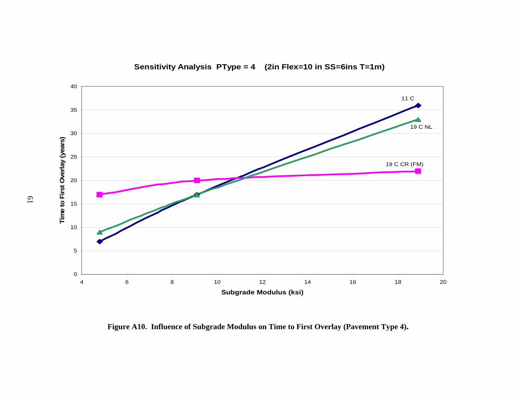
Sensitivity Analysis PType = 4 (2in Flex=10 in SS=6ins T=1m)

0

5

10

15

20

25

30

35

40

4 6 8 10 12 14 16 18 20


Tim

e to

Firs

t Ove

rlay

(yea

rs)

11 C

19 C NL

19 C CR (FM)

Figure A10. Influence of Subgrade Modulus on Time to First Overlay (Pavement Type 4).

61

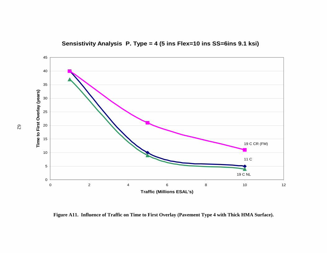
Sensistivity Analysis P. Type = 4 (5 ins Flex=10 ins SS=6ins 9.1 ksi)

0

5

10

15

20

25

30

35

40

45

0 2 4 6 8 10 12

Traffic (Millions ESAL's)

Tim

e to

Firs

t Ove

rlay

(yea

rs)

19 C CR (FM)

11 C

19 C NL

Figure A11. Influence of Traffic on Time to First Overlay (Pavement Type 4 with Thick HMA Surface).

62

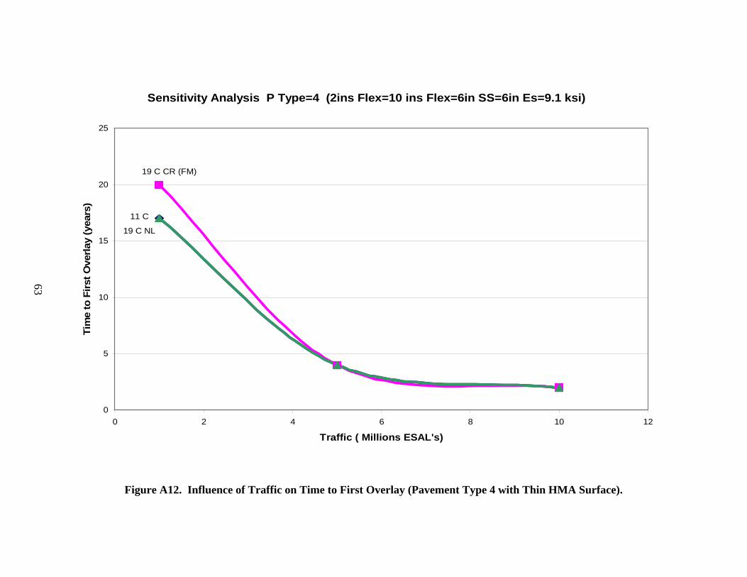
Sensitivity Analysis P Type=4 (2ins Flex=10 ins Flex=6in SS=6in Es=9.1 ksi)

0

5

10

15

20

25

0 2 4 6 8 10 12

Traffic ( Millions ESAL's)

Tim

e to

Firs

t Ove

rlay

(yea

rs)

19 C CR (FM)

11 C

19 C NL

Figure A12. Influence of Traffic on Time to First Overlay (Pavement Type 4 with Thin HMA Surface).

63

Flexible Pavement Design System FPS 19W: User's Manual ... · Flexible Pavement Design System (FPS)...

Documents

Transcript of Flexible Pavement Design System FPS 19W: User's Manual ... · Flexible Pavement Design System (FPS)...