1

Flexible Flow Shop Scheduling Problem to Minimize Makespan with

Renewable Resources

Nariman Abbaszadeh, MSc Student; Department of Industrial Engineering; Babol Noshirvani University of

Technology; Babol; Iran; Mobile: +989376413639

Ebrahim Asadi-Gangraj*, Assistant Professor; Department of Industrial Engineering;Babol Noshirvani University

of Technology; Tel: +981135501814; Mobile: +989112218300

Saeed Emami, Assistant Professor; Department of Industrial Engineering; Babol Noshirvani University of

Technology; Babol; Iran; +981135501818

* Corresponding author; e.asadi@nit.ac.ir

Abstract

This paper deals with a flexible flow shop (FFS) scheduling problem with unrelated parallel machines and

renewable resource shared among the stages. The FFS scheduling problem is one of the most common

manufacturing environment in which there is more than a machine in at least one production stage. In

such a system, to decrease the processing times, additional renewable resources are assigned to the jobs or

machines, and it can lead to decrease the total completion time. For this purpose, a mixed integer linear

programming (MILP) model is proposed to minimize the maximum completion time (makespan) in an

FFS environment. The proposed model is computationally intractable. Therefore, a particle swarm

optimization (PSO) algorithm as well as a hybrid PSO and simulated annealing (SA) algorithm named

SA-PSO, are developed to solve the model. Through numerical experiments on randomly generated test

problems, the authors demonstrate that the hybrid SA-PSO algorithm outperforms the PSO, especially for

large size test problems.

Keywords: Flexible flow shop; MILP model; Renewable resources; Particle swarm optimization;

Simulated annealing

1. Introduction

Scheduling is a resource allocation process to the activities by considering the operational limitations to

optimize one or more objective function. The effective allocation of the resources to the activities leads to

enhance the performance of the manufacturing and service systems, and it is considered as a necessity for

survival in today's competitive market. In the current competitive market, organizations are faced with

new changes every day. Therefore, they must utilize an appropriate scheduling program. It can lead to

effective use of resources, decrease costs, increase efficiency in the production of goods and services, and

satisfy customers’ expectation [1].

Flexible flow shop (FFS) scheduling problem is a developed form of the general flow shop problem

where one or more unrelated parallel machines exist in different stages [2]. Since the FFS scheduling

problem must also determine the jobs allocation to the machines, it is more complex than the flow shop

scheduling problem. In the FFS scheduling problem with unrelated parallel machines, the processing time

of the jobs in each stage is different and dependent on the type of machines. It is considered as one the

difficult production environment due to its high complexity [3].

In the lean production philosophy, it is very important to break the processing bottleneck to enhance

productivity [1]. One of the important issues to achieve this goal is to consider renewable resources to

2

reduce the processing time, especially in the bottleneck stages. It means that the processing time of a job

on a particular machine is dependent on the number of allocated renewable resources. It can lead to

reduce the processing times and finally will decrease the jobs completion time. In the context of

renewable resources, jobs require these resources to process besides the machines. After finishing its

processing, the job returns the allocated resources and they can be used by other jobs on other machines.

By allocating the renewable resources, the jobs processing time is reduced with respect to the number of

allocated renewable resources.

In many real-world manufacturing systems, rather than the machine, renewable resources such as human

resources and molds are available and the shop-floor managers can assign them into the jobs/machines.

Due to the complexity of the scheduling problems with renewable resources, most scheduling approaches

neglect this concept or solve the scheduling problem and renewable resources assignment, separately.

Assigning the renewable resource leads to speed-up the processing operations. It is a critical issue and can

enhance the efficiency of the scheduling problems, and finally, the overall performance of the production

line. As a result, considering this issue is so important in the classical shop scheduling problem. In other

words, considering renewable resources and jobs scheduling, jointly, lead to generating better solutions.

In simultaneous jobs scheduling and renewable resources assignment problem, jobs completion times are

affected by two main decisions: jobs sequencing and scheduling and the optimal assignment of the

renewable resources to each machine in each stage.

There is much application of the FFS scheduling problem with renewable resources in the real world, but

a few research has been examined this problem. In this research, the FFS scheduling problem with

unrelated parallel machines and renewable resources is conducted and an MILP model is developed to

minimize the maximum completion time (makespan). The research problem is computationally

intractable and strongly NP-hard, therefore, two metaheuristic algorithms, including PSO and hybrid SA-

PSO, are developed to solve the research problem.

The outline of the paper is organized as follows: The next section briefly reviews the literature. The

proposed mathematical model is illustrated in Section 3. Section 4 represents the metaheuristic

algorithms, which are proposed to solve the problem. Section 5 gives the obtained results and finally, in

Section 6, a discussion and some suggestions for the future researches are offered.

2. Literature reviews

2.1 Metaheuristic algorithms for flexible flow shop scheduling problems

Due to the NP-hardness of the FFS scheduling problem [4], many researchers proposed different

metaheuristic approaches for this problem. Zabihzadeh and Rezaeian [5] considered an FFS scheduling

problem with release time and robotic transportation. They presented a genetic algorithm (GA) and ant

colony optimization (ACO) for this problem. Karimi, Zandieh, and Karamooz [6] suggested a GA to

solve a multi-objective FFS scheduling problem. Shahvari and Logendran [7] considered a bi-objective

FFS batch scheduling problem with machine-dependent and sequence-dependent family setup times with

various assumptions such as machine availability constraints, ready time, and learning effect. They

presented two stage-based metaheuristic algorithms based on local search and population-based

structures. Almeder and Hartl [8] considered a stochastic FFS scheduling problem with limited buffers.

They proposed a solution approach based on a variable neighborhood search. Besbes, Teghem, and

Loukil [9] focused on the FFS scheduling problem by considering the availability constraints for

machines. They proposed a GA-based approximation algorithm to minimize makespan.

3

Sangsawang et al. [10] dealt with a two-stage reentrant FFS scheduling problem with blocking constraint

and makespan minimization. They developed two hybrid metaheuristic algorithms based on PSO and GA.

The obtained results demonstrate that the hybrid PSO algorithm generates superior results. Jolai et al. [11]

dealt with a bi-objective no-wait two-stage FFS scheduling problem to minimize maximum tardiness and

makespan. They proposed three bi-objective metaheuristic algorithms based on the simulated annealing

algorithm. Akrami, Karimi and Moattar Hosseini [12] proposed GA and Tabu search (TS) for joint

economic lot sizing and scheduling problems in the FFS environment with respect to limited intermediate

buffers.

Marichelvam, Prabaharan, and Yang [13] focused on flexible flow shop scheduling problem with

makespan minimization. They proposed an improved cuckoo search algorithm for this problem. Choong,

Phon-Amnuaisuk, and Alias [14] proposed two hybrid algorithms based on PSO, SA, and TS for the FFS

scheduling problem. Chung and Liao [15] considered an FFS scheduling problem. They proposed an

immunoglobulin-based artificial immune system algorithm to minimize makespan. Dios, Fernandez-

Viagas, and Framinan [16] proposed some heuristic algorithms in the FFS environment to minimize

makespan.

2.2 Scheduling problems with renewable resources

During the last years, various researches have examined renewable resources in the scheduling problems.

Behnamian and Fatemi ghomi [17] considered FFS scheduling problem with resource-dependent

processing times. The selected objective function minimizes the total resource allocation costs and

makespan. They proposed a hybrid metaheuristic algorithm based on GA and a VNS. They compared the

proposed algorithm with the random initial population simulated annealing [18]. The obtained results

demonstrated that the hybrid approach is very efficient for different test problems. Edis and Oguz [19]

studied parallel machine scheduling problem with additional flexible resources to speed-up the production

process. They presented an integer programming (IP) model and IP-based constraint programming for this

problem.

Yin et al. [20] focused on unrelated parallel machines scheduling problem in which resource-dependent

processing time and deteriorating jobs are considered, simultaneously. They proposed a polynomial

approach to minimize a cost-related objective function. Su and Lein [1] dealt with parallel machine

scheduling problem with resource-dependent processing time. The selected objective function aims to

minimize makespan. They firstly proposed a heuristic, named CL, to minimize the makespan and two

procedures, RA1 and RA2, to optimally allocate the renewable resources. Finally, they combined CL with

RA1 and RA2 to solve the problem.

Figielska [21] considered a two-stage flow shop scheduling problem with the parallel machine and

renewable resources in the first stage and single machine in the second stage. He developed a novel

heuristic algorithm to minimize makespan. In Figielska [22], he extended the last research and dealt with

two-stage flow shop scheduling problem with parallel machines on both stages. He proposed four

heuristic algorithms using linear programming to minimize makespan. Figielska [23] also provided three

metaheuristic approaches, TS, SA, and GA, to solve the research problem, considered in Figielska [22].

Li et al. [24] considered scheduling problem in the parallel machine environment with the identical

machine and resource-dependent processing time, so that the processing time is a linearly decreasing

function of the number of allocated resources. They proposed a SA algorithm to achieve near-optimal

solutions. The results showed that the proposed algorithm has good performance in solution quality and

CPU time. Liu and Feng [25] focused on two-stage no-wait flow shop scheduling problem with the cost-

related objective function. They considered position-based and resource-dependent processing time. They

4

decomposed the research problem into the two subproblems, optimal resource allocation, and optimal

sequencing problem. Kellerer [26] presented an approximation algorithm for the identical parallel

machines scheduling problem. He considered resource-dependent processing time with the objective of

makespan minimization.

Jun et al. [27] dealt with a single machine scheduling problem with different assumptions, such as

resource-dependent processing time, learning effect, and serial batch production. They imposed a limited

number of total resources into the model and minimized the makespan. They developed a hybrid

algorithm based on Gravitational Search Algorithm and Tabu Search to achieve high-quality solutions.

Wang and Wang [28] considered the single machine scheduling problem with deteriorating jobs and

convex resource-dependent processing times. They also showed that the research problem is polynomially

solvable with the cost-related objective function.

Wei and Ji [29] focused on a single machine problem with time-dependent and resource-dependent

processing time. They considered different cost-based objective functions for the research problem.

Wang, Wang, and Wang [30] dealt with resource-dependent processing time and learning effect in a

single machine environment. They considered two different processing times functions and developed a

polynomial time algorithm to achieve optimal solutions.

Wang and Cheng [31] considered a single machine environment with respect to resource-dependent

release time and processing time, each of which is a linearly decreasing function of the allocated

resources. The selected objective function is to minimize makespan and the total consumed resource cost.

They also proposed a heuristic approach based on some optimal properties. Nguyen et al. [32] studied

parallel machine scheduling problem with non-renewable resources. They proposed a hybrid approach

based on differential evolution algorithm, iterated greedy search, MILP model, and parallel computing for

this problem.

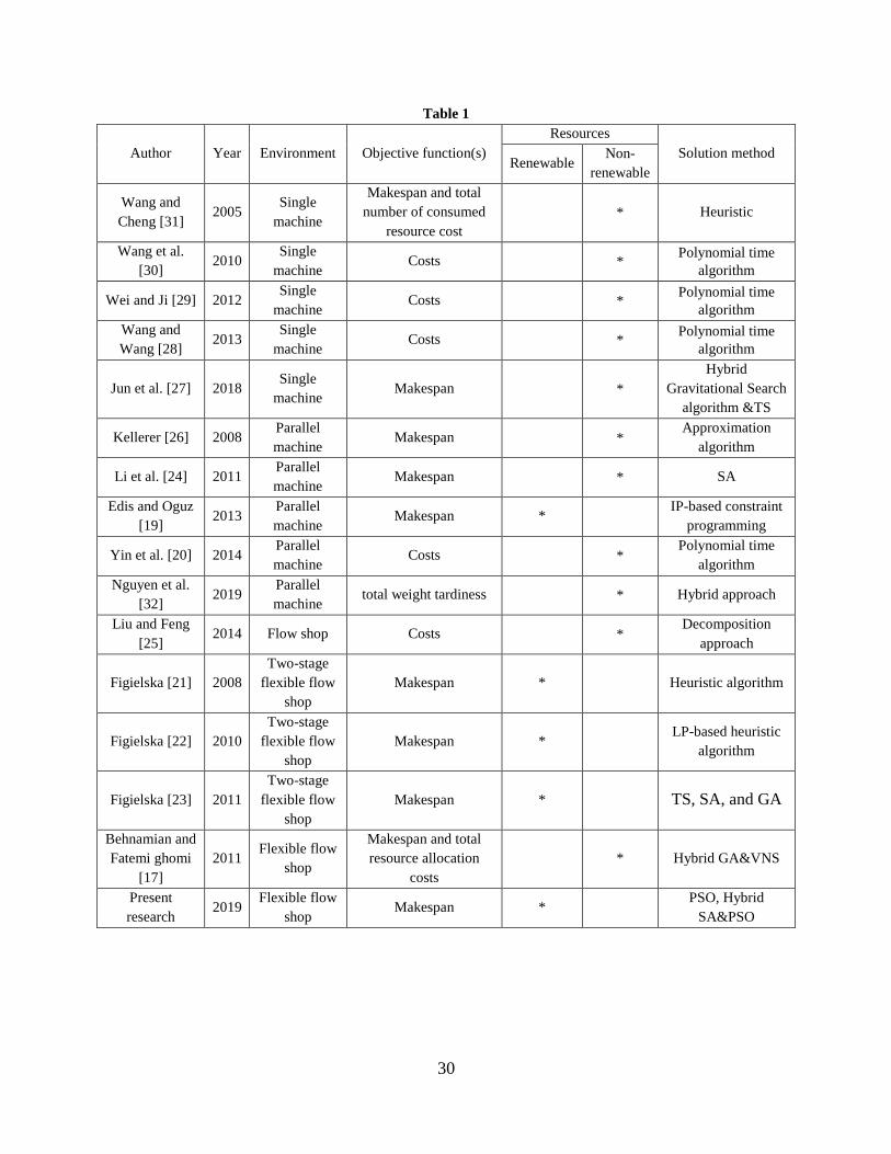
To facilitate the considered papers in the literature review, some of the papers with the background of

renewable resources are categorized in Table 1 with respect to some aspects. They are categorized based

on the type of production environment, objective function, resources (renewable, non-renewable), and

solution method.

Insert Table 1

Regarding Table 1, most of the researches are studied in simple environments such as single machine and

parallel machine environment. Furthermore, only one research considered the multi-stage FFS problem

with non-renewable resources and other researches in this environment focus on two-stage flexible flow

shop. On the other side, none of the reviewed articles addressed the renewable resources in the multi-

stage FFS environment and to the best of our knowledge, considering renewable resources are not

examined in the multi-stage FFS scheduling problem. Moreover, metaheuristic approaches in the context

of renewable resources are rarely studied. As a results, the main contributions of the present research are:

Considering the renewable resources in the FFS scheduling problem

Developing an MILP model for the FFS problem with renewable resources

Proposing two metaheuristic approaches for this problem

Developing a heuristic approach to assign the renewable resources

5

3. Mathematical model of the research problem

This section is devoted to describing the studied problems more formally and introduces the assumptions,

notations, and mathematical model.

3.1 Problem description

As mentioned above, we study an FFS scheduling problem, in which a group of parallel machines is

arranged into a number of stages in series. Assuming that n different jobs require to be processed on

different stages and all the jobs must be processed through the entire stages. There are 𝑚𝑡 unrelated

parallel machines in stage t. Also, a number of renewable resources are considered in this research, which

must be allocated to the machines at each stage. It is assumed that jobs processing times are dependent on

the number of resources allocated to the jobs in each stage. It can lead to speeding up the the processing

of the jobs. The allocation can lead to decreasing the processing times and finally makespan. Regarding

Gupta et al. [33], the normal processing times of the jobs are decreased with respect to the number of

allocated resources and reduction coefficient (see equation 8).

3.2 Problem assumptions

The following assumptions are made in this research:

There is no set-up time for the jobs and travel time between stages.

Entire jobs and machines are available at zero time.

There is no prerequisite constraint between the jobs and they are independent of each other.

There is no possibility of the machines failure.

There is unlimited capacity for the intermediate buffers.

The machines are not the same in the stages (unrelated parallel machines).

All the programming parameters are deterministic.

Each machine in each stage can handle only one job at every time and any job must be allocated

to only one machine in each stage.

The resources are renewable. It means that it can be used for different jobs and stages during the

planning horizon.

3.3 Notations

The following notations are used to formulate the research problem. Indices

𝑡 Index of stages

𝑖 Index of machines

,j j Index of jobs

Parameters

𝑔 Number of stages

𝑚𝑡 Number of unrelated parallel machines in stage 𝑡

𝑛 Number of jobs

t

ijNp Normal processing time of job 𝑗 in stage 𝑡 on machine 𝑖

tR Number of renewable resources in stage 𝑡

6

ta Processing time reduction coefficient in stage 𝑡 due to assigning the renewable resources

t

ijU Maximum renewable resources that can be assigned to job 𝑗 in stage 𝑡 on machine 𝑖

M A large positive number

Decision variables

t

ijp Modified processing time of job 𝑗 on machine 𝑖 in stage 𝑡 after the renewable resources

allocation

t

ijr The number of renewable resources allocated to job 𝑗 in stage 𝑡 on machine 𝑖

t

ijx 1 if job 𝑗 is processed on machine 𝑖 in stage 𝑡; 0 otherwise

t

ijjy 1 if job 𝑗′ precedes job j on machine 𝑖 in stage 𝑡; 0 otherwise

t

jj 1 if completion time jobs j is greater than or equal to start time of job 𝑗′ in stage 𝑡; 0

otherwise

t

jC Completion of job j in stage 𝑡

maxC Makespan

3.4 Mathematical model

(1) maxMin Z C

S.T.

(2) 1, 2,.., ; 1, 2,...,j n t g 11

tm tx

iji

(3) 1, 2,.., ; 1, 2,...,j n t g 11

1 1

1

mp x

ij iji

cj

(4) 1, 2,.., & 2,...,j n t g

1

1tm

t tp xij ij

i

t tc c

j j

(5) ;1, 2,.., 1, 2,..., ; , 1, 2,.., &t

i m t g j j n j j 3 t t ty x xijijj ij

t t t tc M c p x

jj ij ij

(6) ;1, 2,.., 1, 2,..., ; , 1, 2,.., &t

i m t g j j n j j

2 t t ty x xijijj ij

t t t tc M c p x

j ij ijj

(7) 1, 2,..,j n maxg

c Cj

(8) &1, 2,.., 1, 2,.., & 1, 2,...,t

i m j n t g t t t t

p Np a rij ij ij

(9) &1, 2,.., 1, 2,.., & 1, 2,...,

ti m j n t g

t tr Uij ij

(10) 1, 2,..., ; , 1, 2,.., &t g j j n j j 1

*

rmt t t t t

jj j j ij ij

i

M C C p x

7

(11) 1, 2,..., ; , 1, 2,.., &t g j j n j j 1 1 1

1

t tm m nt t t t t

ij ij jj j j

i i j

r r R

(12) ;1, 2,.., 1, 2,..., ; , 1, 2,.., &t

i m t g j j n j j , , {0,1}t t t

ij ijj jjx y

(13) &1, 2,.., 1, 2,.., & 1, 2,...,t

i m j n t g 0,1,2,...t

ijr

(14) &1, 2,.., 1, 2,.., & 1, 2,...,t

i m j n t g max, , 0t t

j ijC p C

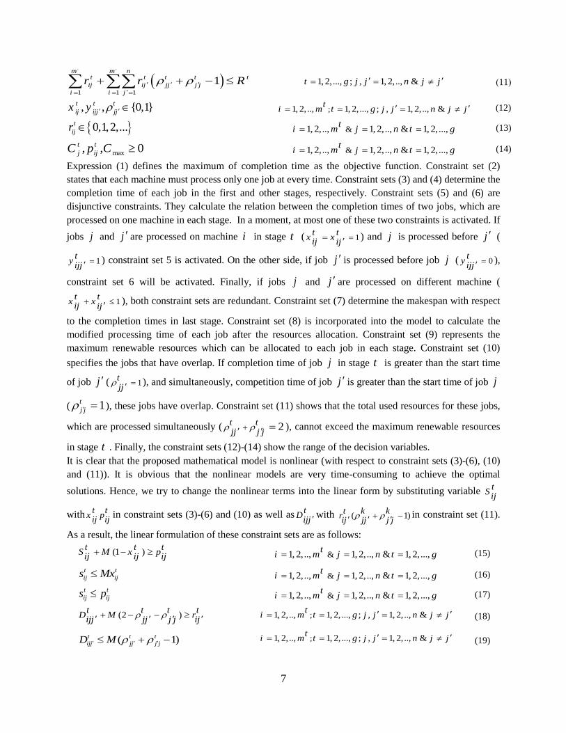
Expression (1) defines the maximum of completion time as the objective function. Constraint set (2)

states that each machine must process only one job at every time. Constraint sets (3) and (4) determine the

completion time of each job in the first and other stages, respectively. Constraint sets (5) and (6) are

disjunctive constraints. They calculate the relation between the completion times of two jobs, which are

processed on one machine in each stage. In a moment, at most one of these two constraints is activated. If

jobs j and j are processed on machine i in stage t ( 1t t

x xij ij

) and j is processed before j (

1t

yijj

) constraint set 5 is activated. On the other side, if job j is processed before job j ( 0

ty

ijj

),

constraint set 6 will be activated. Finally, if jobs j and j are processed on different machine (

1t t

x xij ij

), both constraint sets are redundant. Constraint set (7) determine the makespan with respect

to the completion times in last stage. Constraint set (8) is incorporated into the model to calculate the

modified processing time of each job after the resources allocation. Constraint set (9) represents the

maximum renewable resources which can be allocated to each job in each stage. Constraint set (10)

specifies the jobs that have overlap. If completion time of job j in stage t is greater than the start time

of job j ( 1tjj

), and simultaneously, competition time of job j is greater than the start time of job j

( 1t

j j ), these jobs have overlap. Constraint set (11) shows that the total used resources for these jobs,

which are processed simultaneously ( 2t tjj j j

), cannot exceed the maximum renewable resources

in stage t . Finally, the constraint sets (12)-(14) show the range of the decision variables.

It is clear that the proposed mathematical model is nonlinear (with respect to constraint sets (3)-(6), (10)

and (11)). It is obvious that the nonlinear models are very time-consuming to achieve the optimal

solutions. Hence, we try to change the nonlinear terms into the linear form by substituting variable tS

ij

with t tx p

ij ijin constraint sets (3)-(6) and (10) as well as t

Dijj

with ( 1)t k k

rij jj j j

in constraint set (11).

As a result, the linear formulation of these constraint sets are as follows:

(15) &1, 2,.., 1, 2,.., & 1, 2,...,t

i m j n t g (1 )t t t

S M x pij ij ij

(16) &1, 2,.., 1, 2,.., & 1, 2,...,t

i m j n t g t

ij

t

ij Mxs

(17) &1, 2,.., 1, 2,.., & 1, 2,...,t

i m j n t g t

ij

t

ij ps

(18) ;1, 2,.., 1, 2,..., ; , 1, 2,.., &t

i m t g j j n j j (2 )t t t t

D M rijj jj j j ij

(19) ;1, 2,.., 1, 2,..., ; , 1, 2,.., &t

i m t g j j n j j )1(

t

jj

t

jj

t

jij MD

8

(20) ;1, 2,.., 1, 2,..., ; , 1, 2,.., &t

i m t g j j n j j t

ji

t

jij rD

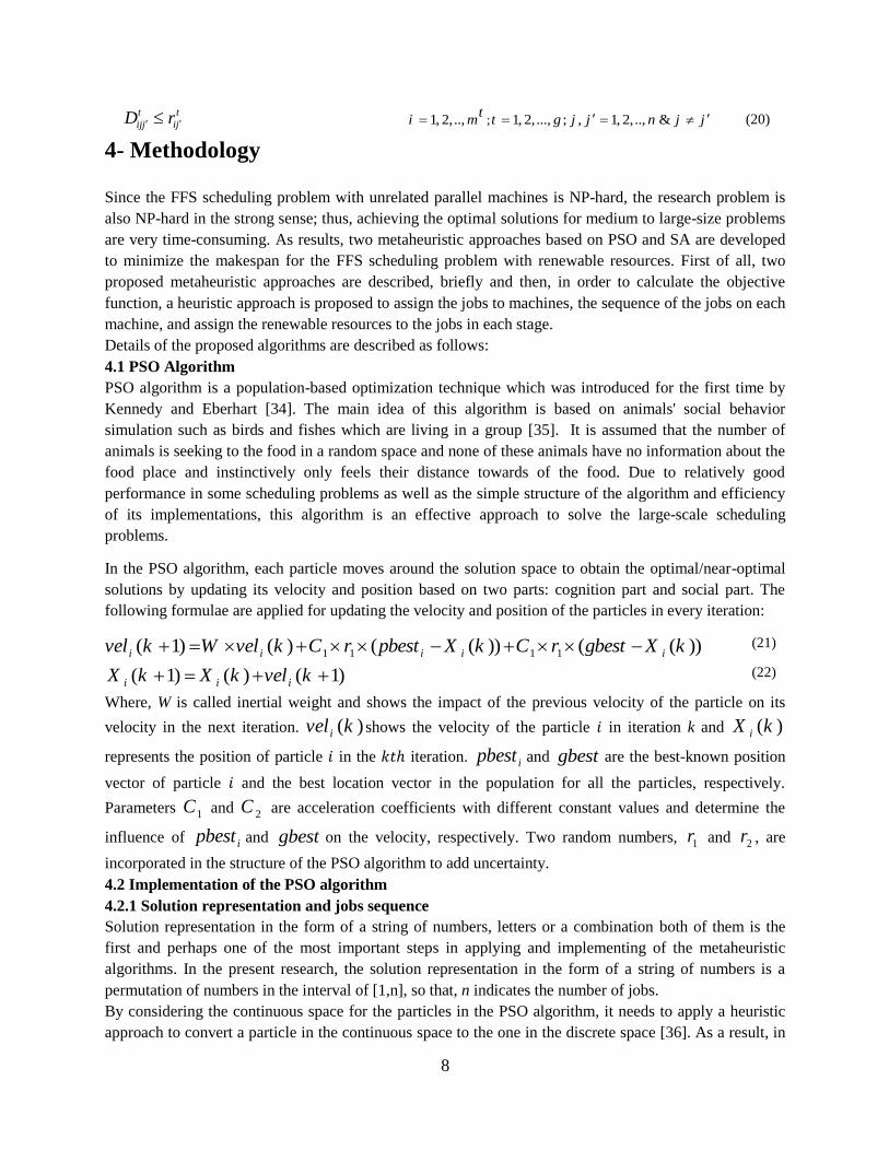
4- Methodology

Since the FFS scheduling problem with unrelated parallel machines is NP-hard, the research problem is

also NP-hard in the strong sense; thus, achieving the optimal solutions for medium to large-size problems

are very time-consuming. As results, two metaheuristic approaches based on PSO and SA are developed

to minimize the makespan for the FFS scheduling problem with renewable resources. First of all, two

proposed metaheuristic approaches are described, briefly and then, in order to calculate the objective

function, a heuristic approach is proposed to assign the jobs to machines, the sequence of the jobs on each

machine, and assign the renewable resources to the jobs in each stage.

Details of the proposed algorithms are described as follows:

4.1 PSO Algorithm

PSO algorithm is a population-based optimization technique which was introduced for the first time by

Kennedy and Eberhart [34]. The main idea of this algorithm is based on animals' social behavior

simulation such as birds and fishes which are living in a group [35]. It is assumed that the number of

animals is seeking to the food in a random space and none of these animals have no information about the

food place and instinctively only feels their distance towards of the food. Due to relatively good

performance in some scheduling problems as well as the simple structure of the algorithm and efficiency

of its implementations, this algorithm is an effective approach to solve the large-scale scheduling

problems.

In the PSO algorithm, each particle moves around the solution space to obtain the optimal/near-optimal

solutions by updating its velocity and position based on two parts: cognition part and social part. The

following formulae are applied for updating the velocity and position of the particles in every iteration:

1 1 1 1( 1) ( ) ( ( )) ( ( ))i i i i ivel k W vel k C r pbest X k C r gbest X k (21)

( 1) ( ) ( 1)i i iX k X k vel k (22)

Where, W is called inertial weight and shows the impact of the previous velocity of the particle on its

velocity in the next iteration. ( )ivel k shows the velocity of the particle 𝑖 in iteration k and ( )iX k

represents the position of particle 𝑖 in the 𝑘𝑡ℎ iteration. ipbest and gbest are the best-known position

vector of particle 𝑖 and the best location vector in the population for all the particles, respectively.

Parameters 1C and 2C are acceleration coefficients with different constant values and determine the

influence of ipbest and gbest on the velocity, respectively. Two random numbers, 1r and 2r , are

incorporated in the structure of the PSO algorithm to add uncertainty.

4.2 Implementation of the PSO algorithm

4.2.1 Solution representation and jobs sequence

Solution representation in the form of a string of numbers, letters or a combination both of them is the

first and perhaps one of the most important steps in applying and implementing of the metaheuristic

algorithms. In the present research, the solution representation in the form of a string of numbers is a

permutation of numbers in the interval of [1,n], so that, n indicates the number of jobs.

By considering the continuous space for the particles in the PSO algorithm, it needs to apply a heuristic

approach to convert a particle in the continuous space to the one in the discrete space [36]. As a result, in

9

this study, Random Key (RK) method [37] is used to transform a particle in continuous space. In the RK

method, the position of any particle in the RK virtual space (continuous space) is turned into a position in

the problem space (discrete space). Consider 5 jobs, the initial sequence vector of the jobs in the

continuous space is as (0.26, 0.53, 0.12, 0.64, 0.85), that is represented in Figure 1, in a given iteration.

Based on the RK method, the numbers in the sequence vector are arranged in descending order with an

index related to each of these numbers. Figure 1 indicates how to achieve the jobs sequence in discrete

space based on the vector in the continuous space. As can be seen, the corresponding sequence of the jobs

is as (1, 2, 4, 5, 3).

Insert Figure 1

4.2.2 Updating the particles

We applied a multiplier χ into the structure of equation (21). It leads to acceleration of the convergence

process and enhances the overall performance of the PSO algorithm [38]. The desired value for χ is

determined as follows:

(23) 1 2 4C C C

(24) 2

2

2 4C C C

According to the above equation, the position and velocity of the particles will be updated based on the

following formulae:

(25) 1 1 1 1( 1) ( ) ( ( )) ( ( ))i i i i ivel k W vel k C r pbest X k C r gbest X k

(26) ( 1) ( ) ( 1)i i iX k X k vel k

Similar to Tadayon and Salmasi [39], we applied Eq. (27) to determine the value of w in each iteration. If

w is set to a high value at the beginning of the procedure and gradually reducing w to a lower value, better

performance of the PSO algorithm can be obtained.

(27) max min

max

( )W W iterW W

MaxIt

In which, maxW and minW are the upper and lower bounds for W, respectively, and MaxIt is the total

number of iterations that accomplished in the PSO algorithm.

The pseudo-code of the PSO approach which is applied in this research is presented in Figure 2:

Insert Figure 2

4.3 Simulated Annealing Algorithm

Simulated annealing (SA) algorithm, or in other words, the fusion/cooling algorithm was provided in the

early 1980s by Kirkpatrick, Gelatt, and Vecci [40]. During the simulated annealing process, a material is

10

heated to a temperature so that it is higher than its melting temperature and then, it gradually is lowering

its temperature. The temperature reduction process is so slow and it is to some extent that this material is

in thermodynamic equilibrium. In other words, in any created temperature, the atoms can be replaced only

to the extent that to create the greatest stability, this means that if the material is cooled with more slowly,

so the atoms will be able to release greater energy and locating in the direction of the greatest stability.

SA algorithm is one of the first metaheuristic methods for searching neighborhood solutions that is having

an explicit strategy to avoid being trapped in the local optimum solutions. In this approach, if the current

solution has a better objective value than the last one, the current solution is accepted for the next

iteration. Otherwise, it will be accepted as the current solution with respect to the Boltzmann function if:

(28) ( ( )) ( ( 1))exp k kf X t f X t

PT

Where, P is a random number in the interval [0,1], ( ( ))kf X t is the objective value of the solutions in

the current iteration (t), ( ( 1))kf X t is the objective value of the current in the previous iteration and T

is called as the temperature at which the current solution is evaluated. Note that, T is a function of two

input parameters: initial temperature and cooling rate [41].

4.4 Hybrid SA-PSO algorithm

Although the PSO algorithm has relatively good performance in the optimization problems, especially in

scheduling problems, one of the major drawbacks of this algorithm is that it is easy to trap in the local

optimum. Therefore, a combination of the PSO with other algorithms such as SA can solve this difficulty.

As mentioned above, the SA algorithm is one of the well-known metaheuristic algorithms to search the

neighborhood solutions, such that it applies a high-performance strategy to prevent trapping in local

optimum solutions. For this reason, in this research, a hybrid algorithm based on the PSO and SA, namely

SA-PSO algorithms is proposed.

In the proposed procedure, if the gbest ( pbest ) of a particle has better performance (objective

function), the new particle will be accepted, but if the gbest ( pbest ) is inferior, we may still accept it

with a positive probability, based on Boltzmann function (Eq. 28).

The pseudo-code of the hybrid SA-PSO algorithm is presented in Figure 3:

Insert Figure 3

4.5 Calculation the objective function

One of the most important aspects of the metaheuristic approaches is to calculate the objective function

based on the proposed solution representation. For this purpose, a heuristic approach is proposed, here.

Due to the FFS environment with unrelated parallel machines and renewable resources in this research,

we must make three decision to calculate the objective function: 1) Assign the jobs to each machine in

each stage, 2) Determine the jobs sequence on each machine and 3) Allocate the renewable resources to

the machines.

The details of the proposed approach are discussed as bellows:

Step 1: Scheduling of the jobs in the first stage

11

By considering the obtained jobs sequence based on the RK method, the jobs are allocated to all the

machines (available or unavailable) at the first stage and completion times of the jobs are calculated. In

this research, each job is virtually allocated to all the machines in the first stage and the machine with

minimum completion time is selected and the job is really assigned to this machine.

Step 2: Scheduling of the jobs in other stages

For the second stage until the end, the jobs are sorted in the ascending order of the completion time on the

previous stage. Afterward, the jobs are allocated to all the machines (available or unavailable) and the

machine with minimum completion time is selected to assign the job. By considering this procedure for

entire stages, the completion time of the last jobs is calculated and considered as 𝐶𝑚𝑎𝑥.

Step 3: Allocation of the renewable resources

As mentioned before, by allocating a fixed number of renewable resources to the machines, the job

processing time is reduced regarding the normal processing time and coefficient of processing time

reduction. In this issue, the resources allocation to the machines is conducted after the jobs assigning to

the machines and jobs sequencing on the machines at each stage. First of all, scheduling of the jobs is

performed by the normal processing time without considering any renewable resources. After that, the

critical path on the Gantt chart, which determines 𝐶𝑚𝑎𝑥, is identified and one renewable resource (if

available) is assigned to the jobs on the critical path in each stage. Then, the new 𝐶𝑚𝑎𝑥 is determined

based on the new processing time. The above procedure is continued until entire renewable resources are

assigned to the jobs.

A simple example: In order to how the job scheduling is generated based on the proposed heuristic

approach in the FFS problem with renewable resources, a simple example is considered, here. Suppose

that there is a scheduling problem with five jobs, two, two, and one renewable resources in stage 1, 2, and

3, respectively, two machines in each stage, and 1; 1, 2, 3tt

a . The processing times of the jobs are

produced randomly in the interval [2,10]. Table 2 shows the normal processing time of any job on

different machines in any stage.

Insert Table 2

It is assumed that the proposed metaheuristic approach generates a vector for the jobs sequence as J= (0.5,

0.2, 0.3, 0.8, 0.9) in a given iteration. The equivalent sequence vector generated by the RK method should

be: Seq=(5, 4, 1, 3, 2).

As mentioned above, in order to assign the jobs to each machine in any stage, a job in the sequence is

assigned to all the available and unavailable machines in each stage and a machine with the earliest

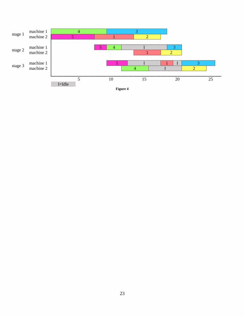
completion time is selected. As a result, the Gant chart of the generated solution based on the proposed

procedure (step 1, 2 in the heuristic approach) is shown in Figure 4.

Insert Figure 4

Regarding to Figure 4, the initial makespan (without renewable resources assignment) equals to 25.

In step 3 of the heuristic approach, the renewable resources must be assigned to the jobs to reduce the

processing times and as a result, reduce the makespan. As can be seen in Figure 3, the critical path on the

𝐶𝑚𝑎𝑥 is jobs 4 and 3 on machine 1 at first stage, job 3 on machine 1 at the second stage, and finally, job 3

12

on machine 1 at the last stage. Regarding the number of renewable resources in each stage and constraint

set (10), the processing time of the jobs on the critical path is reduced by one unit. As a result, the Gant

chart of the new sequence is changed as follow:

Insert Figure 5

As a result, the new maxC with one renewable resource is as 24.

In iteration 2, there is one renewable resource for the first and second stages; therefore, we only consider

the jobs on the critical path in theses stages. Therefore, regarding the Figure 5, the critical path is jobs 5,

1, and 2 on machine 2 at the first stage and job 2 on machine 2 at the second stage. By reducing one unit

of the processing time of the jobs on the critical path in the first and second stages, the new Gant chart is

shown in Figure 6:

Insert Figure 6

Figure 6 shows that final maxC with two, two, and one renewable resource for the first, second, and last

stages is equal to 22.

4.6 Improvement of the proposed algorithms

In order to improve the performance of the proposed algorithms, a local search scheme is incorporated

into the metaheuristic algorithms. The local search finds entire neighborhoods of each particle by

substituting every two jobs in the sequence vector. After that, the objective function of each particle is

calculated and it is substituted by the best neighbor and the position vector is changed by the best

neighbor. The proposed local search scheme is done on the 𝑔𝑏𝑒𝑠𝑡 in each iteration.

5. Computational results

In this section, some numerical experiments are designed to investigate validation of the mathematical

model. Furthermore, the performance of the proposed algorithms is investigated by comparing them with

the optimal solutions and with each other. In this section, two different experiments are conducted for this

purpose. At first, the performance of the proposed metaheuristic approaches is evaluated by comparing

with the optimal solutions through the small-size test problems. Afterward, we compare the performance

of the proposed metaheuristic approaches with each other based on medium to large-size test problems.

Optimal solutions of the test problems obtained by Lingo 9.0 software and the proposed metaheuristic

algorithms were implemented in MATLAB and tested on a computer with 2.4 GHz CPU and 3 GB of

RAM.

5.1 Comparison of the proposed metaheuristic algorithms with the optimal solutions

This section is dedicated to evaluate the performance of the proposed metaheuristic algorithms by

comparing them with optimal solutions, which are obtained by the proposed MILP model. Regarding the

NP-hardness of the FFS scheduling problem with renewable resources, test problems are limited to the

small size. For this purpose, 15 test problems have designed in small size to compare the mathematical

model with the metaheuristic algorithms. In order to generate small-size test problems, five characteristics

are used to typify the test problems. They are the number of jobs, normal processing time, number of

13

stages, number of machines in each stage, and number of renewable resources. Test problem

characteristics are summarized in Table 3:

Insert Table 3

Based on the test problems characteristics, 15 test problems with different size are generated and each of

them is solved by Lingo 9.0 software with a time limit of 3600 seconds. Their performance is evaluated in

terms of CPU Time and Optimal GAP, which is determined as follow:

(29) max 100

C Optimal solutionOptimal Gap

Optimal solution

In which, maxC and Optimal solution show the maximum completion time, generated by the

metaheuristic algorithms and MILP model, respectively. It is necessary to mention that the local search

scheme has a significant influence on the performance of the original PSO and improves its performance.

Insert Table 4

By considering Table 4, the PSO and SA-SPO algorithms have solved 9 and 11 out of 15 problems,

optimally. Furthermore, the average optimal gap for both metaheuristic approaches is 3.0% and 1.2%,

respectively. Moreover, the average CPU time to achieve the optimal solution in different test problem by

the MILP model, PSO, and SA-PSO algorithms is equal to 379.1, 2.77 and 7.93, respectively. Thus, we

can conclude that both proposed metaheuristic algorithms are able to generate optimal/near-optimal

solutions in a reasonable time. By considering the optimal gap column in Table 4, it is observed that the

solutions which are presented by the SA-PSO algorithm have better quality.

5.2 Comparison of the metaheuristic algorithms for medium to large-size test problems

This section is devoted to compare the performance of the proposed metaheuristic algorithms based on

some test problems. Regarding NP-hardness of the FFS scheduling problem with renewable resources, the

proposed MILP model cannot achieve the optimal solutions in a reasonable time for medium to large-size

test problems. Therefore, we only compare the metaheuristic algorithm with each other. In order to

generate the test problems, different levels of the test problems characteristics are summarized in Table 5.

Insert Table 5

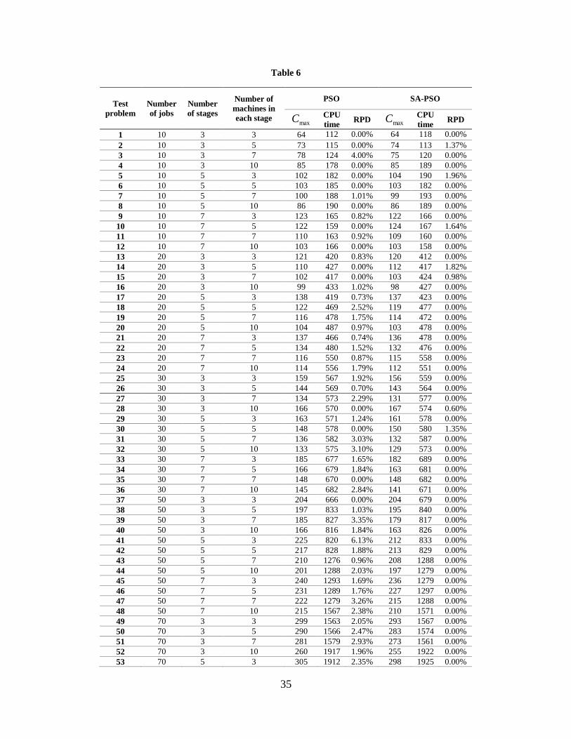
For evaluation purposes, 72 test problems are randomly generated based on Table 5. Two criteria, CPU

Time (Sec.) and relative percentage deviation (RPD), are used to compare the proposed algorithms. The

RPD is determined as follow:

(30) max max

max

( )100

( )

C best CRPD

best C

14

Where maxC is the objective value that is obtained by a given algorithm and max( )best C is the best

solution that is obtained from both algorithms. The obtained results are presented in Table 6:

Insert Table 6

The average CPU time and RPD in each group of test problems that are obtained by the PSO and SA-PSO

algorithms in Table 6 are presented in Table 7.

Insert Table 7

As can be seen in Table 7, the hybrid SA-PSO provides better results than the PSO algorithm based on

the average RPD. Furthermore, the average CPU time of both algorithms in each group of test problems is

approximately similar to each other.

For more scrutiny and as a formal comparison, the performance of the proposed algorithms is compared,

statistically. Figure 7 shows the means plot and least significant difference (LSD) intervals (at the 95 %

confidence level) for the algorithms.

Insert Figure 7

The results demonstrate that the SA-PSO algorithm statistically outperforms the PSO algorithm at the

95% confidence level.

In order to evaluate the effects of different controllable parameters of the test problems, average RPD plot

for the controllable parameters is depicted, here. As results, we consider the number of jobs, the number

of stages, and the number of machines in each stage as controllable parameters.

The number of jobs: The interaction between the type of algorithms and the number of jobs is depicted in

Figure 8 based on the average RPD.

Insert Figure 8

It can be seen that, in small size problems, both algorithms have similar performance, but for the larger

size test problems, there is a significant difference between the proposed algorithms.

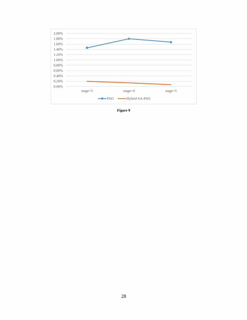
The number of stages: the average RPD plot to consider the effect of the number of stages on the quality

of the proposed algorithms is depicted in Figure 9.

Insert Figure 9

Figure 10 shows that the SA-PSO algorithm works better than the PSO algorithm in all the cases.

15

The number of machines in each stage: another average RPD plot is used to see the effect of the number

of machines in each stage on the performance of the proposed algorithms, (see Figure 10).

Insert Figure 10

Regarding Figure 10, we can also conclude that, the SA-PSO algorithm shows the best performance in all

cases.

6. Conclusions and future researches

In this study, we studied the effect of renewable resources in the flexible flow shop scheduling problem

with unrelated parallel machines. Assignment of the renewable resources to the machines can lead to

decreasing the makespan. For this purpose, a mixed integer linear programming model is proposed to

minimize the makespan in an FFS environment with renewable resources. The proposed model was

computationally NP-hard, therefore, a PSO algorithm, as well as a hybrid SA-PSO algorithm, are

proposed to solve the model. The obtained results from the randomly generated test problems show that

the SA-PSO algorithm outperforms the PSO in both small and large size problems.

Suggestions for future studies include considering other objective functions such as cost-related and due

date-related objective functions. Other clues for the future researches are the consideration of release time

and machine availability constraints, and batch processing. Also, other production environment, such as

job shop and flexible job shop can be considered in the future studies. Hybridization other well-known

metaheuristic approaches, such as genetic algorithm (GA), variable neighborhood search (VNS), and tabu

search (TS) can be considered as the future research.

Acknowledgment

The second author would like to thank the financial support of the Babol Noshirvani University of

Technology for this research under grant number BNUT/388026/98.

7. References

1. Su, L., and Lien, C. “Scheduling parallel machines with resource-dependent processing times”,

Int. J. Prod. Res. 117, 256–266 (2009).

2. Gholami, H.R., Mehdizadeh E., Naderi, B. “Mathematical models and an elephant herding

optimization for multiprocessor-task flexible flow shop scheduling problems in the

manufacturing resource planning (MRPII) system”. Sci. Iran. doi:

10.24200/SCI.2018.5552.1343 (2018).

3. Ebrahimi, M., Fatemi Ghomi, S.M.T and Karimi, B. “Hybrid flow shop scheduling with

sequence dependent family setup time and uncertain due dates”, Appl. Math. Model. 38, 2490-

2540 (2014).

4. Asadi-Gangraj, E. “Lagrangian relaxation approach to minimize makespan for hybrid flow shop

scheduling problem with unrelated parallel machines”, Sci. Iran. 5, 3765-3775 (2018).

5. Zabihzadeh, S.S., and Rezaeian, J. “Two meta-heuristic algorithms for flexible flow shop

scheduling problem with robotic transportation and release time”, Appl. Soft. Comput. 30, 319-

330 (2016).

16

6. Karimi, N., Zandieh, M. and Karamooz, H.R. “Bi-objective group scheduling in hybrid flexible

flowshop: a multi-phase approach”, Expert. Syst. Appl. 37, 4024-4032 (2010).

7. Shahvari, O. and Logendran, R. “A comparison of two stage-based hybrid algorithms for a batch

scheduling problem in hybrid flow shop with learning effect”, Int. J. Prod. Econ. 195, 27-248

(2018).

8. Almedera, C. and Hartl, R.F. “A metaheuristic optimization approach for a real-world stochastic

flexible flow shop problem with limited buffer”, Int. J. Prod. Econ. 145, 88-95 (2013).

9. Besbes, W., Teghem, J., and Loukil, T. “Scheduling hybrid flow shop problem with non-fixed

availability constraints”, Eur. J. Ind. Eng. 4, 413-433 (2010).

10. Sangsawang, C., Sethanan, K., Fujimoto, T., and Gen, M. “Metaheuristics optimization

approaches for two-stage reentrant flexible flow shop with blocking constraint”, Expert. Syst.

Appl. 42, 2395-2410 (2015).

11. Jolai, F., Asefi, H., Rabiee, M. and Ramezani, P. “Bi-objective simulated annealing approaches

for no-wait two-stage flexible flow shop scheduling problem”, Sci. Iran. 20, 861-872 (2013).

12. Akrami, B., Karimi, B. and Moattar Hosseini, S.M. “Two metaheuristic methods for the

common cycle economic lot sizing and scheduling in flexible flow shops with limited

intermediate buffers: The finite horizon case”, Appl. Math. Comp. 183, 634-645 (2006).

13. Marichelvam, M.K., Prabaharan, T. and Yang, X.S. “Improved cuckoo search algorithm for

hybrid flow shop scheduling problems to minimize makespan”, Appl. Soft. Comput. 19, 93-101

(2014).

14. Choong, F., Phon-Amnuaisuk, S. and Alias, M.Y. “Metaheuristic methods in hybrid flow shop

scheduling problem”, Expert. Syst. Appl. 38, 10787-10793 (2011).

15. Chung, T., and Liao, C. “An immunoglobulin-based artificial immune system for solving the

hybrid flow shop problem”, Appl. Soft. Comput. 13, 3729-3736 (2013).

16. Dios, M., Fernandez-Viagas, V., and Framinan, J.M. “Efficient heuristics for the hybrid flow

shop scheduling problem with missing operations. Comput. Ind. Eng. 115 (2018) 88-99.

17. Behnamian, J., and Fatemi Ghomi, S.M.T. “Hybrid flowshop scheduling with machine and

resource-dependent processing times”, Appl. Math. Model. 35, 1107-1123 (2011).

18. Jungwattanakit, J., Reodecha, M., Chaovalitwongse, P., and Werner, F.A. “Comparison of

scheduling algorithms for flexible flow shop problems with unrelated parallel machines, setup

times, and dual criteria”, Comput. Oper. Res. 36, 358–378 (2009).

19. Edis, E.B., Oguz, C. “Parallel machine scheduling with flexible resources”, Comput. Ind. Eng.

63, 433–447 (2009).

20. Yin, N., Kang, L., Sun, T., Yue, C., and Wang, X. “Unrelated parallel machines scheduling with

deteriorating jobs and resource dependent processing times”, Appl. Math. Model. 38, 4747-4755

(2014).

21. Figielska, E. “A new heuristic for scheduling the two-stage flowshop with additional resources”,

Comput. Ind. Eng. 54, 750-763 (2008).

22. Figielska, E. “Heuristic algorithms for preemptive scheduling in a two-stage hybrid flowshop

with additional renewable resources at each stage” Comput. Ind. Eng. 59, 509-519 (2010).

23. Figielska, E. “Linear programming & metaheuristic approach for scheduling in the hybrid

flowshop with resource constraints”, Control. Cybern. 4, 1209-1230 (2011).

24. Li, K., Shi, Y., Yang, S. and Cheng, B. “Parallel machine scheduling problem to minimize the

makespan with resource dependent processing times”, Appl. Soft. Comput. 11, 5551-5557

(2011).

25. Liu, Y., and Feng, Z. “Two-machine no-wait flowshop scheduling with learning effect and

convex resource-dependent processing times”, Comput. Ind. Eng. 75, 170-175 (2014).

26. Kellerer, H. “An approximation algorithm for identical parallel machine scheduling with

resource dependent processing times”, Oper. Res. Lett. 36, 157-159 (2008).

17

27. Jun, P., Xinbao, L., Baoyu, L., Pardalos, P.M., and Min, K. “Single-machine scheduling with

learning effect and resource-dependent processing times in the serial-batching production”,

Appl. Math. Model. 58, 245-253 (2018). 28. Wang, X., and Wang, J. “Single-machine scheduling with convex resource dependent processing

times and deteriorating jobs”, Appl. Math. Model. 37, 2388-2393 (2013).

29. Wei, C., and Ji, P. “Single-machine scheduling with time-and-resource-dependent processing

times”, Appl. Math. Model. 36, 792-798 (2012).

30. Wang, D., Wang, M., and Wang, J., “Single-machine scheduling with learning effect and

resource-dependent processing times”, Comput. Ind. Eng. 59, 458-462 (2010).

31. Wang, X., and Cheng, T.C.E. “Single machine scheduling with resource dependent release times

and processing times”, Eur. J. Oper. Res. 162, 727-739 (2005).

32. Nguyen, S., Thiruvady, D., Ernst, A.T., and Alahakoon, D. “A Hybrid Differential Evolution

Algorithm with Column Generation forResource Constrained Job Scheduling”, Comput. Oper.

Res. Doi: https://doi.org/10.1016/j.cor.2019.05.009 (2019).

33. Gupta, J.N.D., Kruger, K., Lauff, V., Werner, F., and Sotskov, Y.N. “Heuristics for hybrid flow

shops with controllable processing times and assignable due dates”, Comput. Oper. Res. 29

1417–1439 (2002).

34. Kennedy, J., and Eberhart, R.C. “Particle swarm optimization”, Proceedings of the IEEE

International Conference on Neural Networks, 4, 1942–1948 (1995).

35. Poonthalir, G., Nadarajan, R. and Geetha, S. “Vehicle routing problem with limited refueling

halts using particle swarm optimization with greedy mutation operator”, RAIRO-Oper. Res. 49,

689-716 (2015).

36. Nayeri, S., Asadi-Gangraj, E., Emami, S. “Metaheuristic algorithms to allocate and schedule of

the rescue units in the natural disaster with fatigue effect”. Neural Comput. Appl. Doi:

https://doi.org/10.1007/s00521-018-3599-6 (2018).

37. Bean, J.C. “Genetics and random keys for sequencing and optimization”, ORSA J. Comput. 6,

154–160 (1994).

38. Poli, R. and Kennedy, J. and Blackwell, T. “Particle swarm optimization: an overview”, Swarm.

Intell. 1, 33–57 (2007).

39. Tadayon, B., and Salmasi, N. “A two-criteria objective function flexible flowshop scheduling

problem with machine eligibility constraint”, Int. J. Adv. Manuf. Tech. 64, 1001-1015 (2013).

40. Kirkpatric, S. and Gelatt, C.D., and Vecci, M.P. “Optimization by simulated annealing”, Sci.

220, 671–680 (1983).

41. Asadi-Gangraj, E., and Nahavandi, N. “A metaheuristic approach for batch sizing and

scheduling problem in flexible flow shop with unrelated parallel machines”, Int. J. Comp. App.,

97, 31-36 (2014).

18

Biographies

Nariman Abbaszadeh received his BS degree in Industrial Engineering from Mazandaran University of

Science and Technology and MS degree in Industrial Engineering from Babol Noshirvani University of

Technology, Babol, Iran. His research interests include operations research, sequencing and scheduling,

and production planning.

Ebrahim Asadi-Gangraj received his BS degree in Industrial Engineering from Isfahan University of

Technology, Isfahan, Iran, in 2005; MS degree in Industrial Engineering from the Tarbiat Modares

University in 2008; and PhD degree in Industrial Engineering from the Tarbiat Modares University, Iran,

in 2014. He is currently Assistant Professor of Industrial Engineering at Babol Noshirvani University of

Technology, Babol, Iran. His research interests include applied operations research, sequencing and

scheduling, production planning, and supply chain management.

Saeed Emami is an Assistant Professor at the Department of Industrial Engineering, Babol Noshirani

University of Technology, Babol, Iran. He received his BS, MSc, and PhD in Industrial Engineering from

Isfahan University of Technology, Isfahan, Iran. His research interests are operations research, robust

optimization, production planning and scheduling.

19

Figure captions

Figure 1. Random key method

Figure 2. The pseudo-code of the proposed PSO algorithm

Figure 3. The pseudo-code of the SA-PSO algorithm

Figure 4. The Gant chart with the normal processing time

Figure 5. The Gant chart in iteration 1

Figure 6. The Gant chart in iteration 2

Figure 7. The means plot and least significant difference (LSD) intervals

Figure 8. The interaction between the type of algorithms and the number of jobs

Figure 9. The interaction between the type of algorithms and the number of stages

Figure 10. The interaction between the type of algorithms and the number of machines in each stage

Table captions

Table 1. Different aspects of the related researches

Table 2. The normal processing time of each job

Table 3. Test problems characteristics of the small size test problems

Table 4. Comparison of the metaheuristic algorithms with optimal solutions

Table 5. Information related to the medium to large-size test problems

Table 6. Computational results of PSO and SA-PSO algorithms on medium and large size test problems

Table 7. The average CPU time and RPD in each group of test problems in medium and large size

problems

20

Index 1 2 3 4 5

Particle 0.85 0.64 0.12 0.53 0.26

Descending Order 0.85 0.64 0.53 0.26 0.12

Jobs sequence 1 2 4 5 3

Figure 1

21

Initialization

Population size (𝑝𝑜𝑝 − 𝑠𝑖𝑧𝑒); Maximum number of iterations (𝑀𝑎𝑥𝐼𝑡); Maximum

velocity (𝑉𝑚𝑎𝑥); Learning factors (𝑐1 and 𝑐2); Constriction coefficient (𝜒)

Generate the initial particles based on 𝑝𝑜𝑝 − 𝑠𝑖𝑧𝑒 and 𝑡 = 1

While 𝑡 ≤ 𝑀𝑎𝑥𝐼𝑡 Do

Calculate fitness value for every particle

Evaluate the initial particles to get the local best (𝑝𝑏𝑒𝑠𝑡) and the global best (𝑔𝑏𝑒𝑠𝑡):

If 𝐹𝑘𝑡 < 𝐹𝑘

𝑝𝑏𝑒𝑠𝑡 → 𝑝𝑏𝑒𝑠𝑡𝑘(𝑡) = 𝑋𝑘(𝑡)

If 𝐹𝑘𝑝𝑏𝑒𝑠𝑡

< 𝐹𝑔𝑏𝑒𝑠𝑡 → 𝑔𝑏𝑒𝑠𝑡(𝑡) = 𝑝𝑏𝑒𝑠𝑡𝑘(𝑡)

Update the velocity and position of each particle

t=t+1

End While

Figure 2

22

Initialization

Population size (𝑝𝑜𝑝 − 𝑠𝑖𝑧𝑒); Maximum number of iterations (𝑀𝑎𝑥𝐼𝑡); maximum

velocity (𝑉𝑚𝑎𝑥); Learning factors (𝑐1 and 𝑐2); Constriction coefficient (𝜒); Initial

temperature(𝑇0) ; Cooling rate (𝛼)

Generate the initial particles based on 𝑝𝑜𝑝 − 𝑠𝑖𝑧𝑒 and t=1

While 𝑡 ≤ 𝑀𝑎𝑥𝐼𝑡 Do

Calculate fitness value for every particle

Evaluate the initial particles to get the local best (𝑝𝑏𝑒𝑠𝑡) and the global best (𝑔𝑏𝑒𝑠𝑡):

If 𝐹𝑘𝑡 < 𝐹𝑘

𝑝𝑏𝑒𝑠𝑡 → 𝑝𝑏𝑒𝑠𝑡𝑘(𝑡) = 𝑋𝑘(𝑡)

Else

Calculate ∆= 𝐹𝑘𝑡 − 𝐹𝑘

𝑝𝑏𝑒𝑠𝑡

Generate a random number 𝑟 ∈ (0,1)

If 𝑟 ≤ ( 𝑝 = 𝑒−∆

𝑇 ) →𝑝𝑏𝑒𝑠𝑡𝑘(𝑡) = 𝑋𝑘(𝑡)

If 𝐹𝑘𝑝𝑏𝑒𝑠𝑡

< 𝐹𝑔𝑏𝑒𝑠𝑡 → 𝑔𝑏𝑒𝑠𝑡(𝑡) = 𝑝𝑏𝑒𝑠𝑡𝑘(𝑡)

Else

Calculate ∆= 𝐹𝑘𝑝𝑏𝑒𝑠𝑡

− 𝐹𝑔𝑏𝑒𝑠𝑡

Generate a random number r∈(0,1)

if 𝑟 ≤ ( 𝑝 = 𝑒−∆

𝑇 ) →𝑔𝑏𝑒𝑠𝑡(𝑡) = 𝑝𝑏𝑒𝑠𝑡𝑘(𝑡)

Update the velocity and position of each particle

Reduce the temperature 𝑇𝑡 = 𝛼(𝑇𝑡−1)

t=t+1

End While

Figure 3

23

stage 1 machine 1 4 3

machine 2 5 1 2

stage 2

machine 1

5 4 I 3

machine 2

1 2

stage 3

machine 1

5 I 1 I 3

machine 2

4 I 2

5

10

15

20

25

I=Idle

Figure 4

24

stage 1 machine 1 4 3

machine 2 5 1 2

stage 2

machine 1

5 4 I 3

machine 2

1 2

stage 3

machine 1

5 I 1 3

machine 2

4 I 2

5

10

15

20

24

I=Idle

Figure 5

25

stage 1 machine 1 4 3

machine 2 5 1 2

stage 2

machine 1

5 I 4 I 3

machine 2

1 2

stage 3

machine 1

5 I 1 I 3

machine 2

4 I 2

5

10

15

20

22

I=Idle

Figure 6

26

Hybrid SA-PSOPSO

2.00%

1.50%

1.00%

0.50%

0.00%

Ave

rag

e R

PD

95% CI for the Mean

Interval Plot of PSO and SA-PSO

Figure 7

27

Figure 8

0.00%

0.50%

1.00%

1.50%

2.00%

2.50%

3.00%

job=10 job=20 job=30 job=50 job=70 job=100

PSO Hybrid SA-PSO

28

Figure 9

0.00%

0.20%

0.40%

0.60%

0.80%

1.00%

1.20%

1.40%

1.60%

1.80%

2.00%

stage=3 stage=4 stage=5

PSO Hybrid SA-PSO

29

Figure 10

0.00%

0.50%

1.00%

1.50%

2.00%

2.50%

machine=3 machine=5 machine=7 machine=9

PSO Hybrid SA-PSO

30

Table 1

Author Year Environment Objective function(s)

Resources

Solution method Renewable

Non-

renewable

Wang and

Cheng [31] 2005

Single

machine

Makespan and total

number of consumed

resource cost

* Heuristic

Wang et al.

[30] 2010

Single

machine Costs *

Polynomial time

algorithm

Wei and Ji [29] 2012 Single

machine Costs *

Polynomial time

algorithm

Wang and

Wang [28] 2013

Single

machine Costs *

Polynomial time

algorithm

Jun et al. [27] 2018 Single

machine Makespan *

Hybrid

Gravitational Search

algorithm &TS

Kellerer [26] 2008 Parallel

machine Makespan *

Approximation

algorithm

Li et al. [24] 2011 Parallel

machine Makespan * SA

Edis and Oguz

[19] 2013

Parallel

machine Makespan *

IP-based constraint

programming

Yin et al. [20] 2014 Parallel

machine Costs *

Polynomial time

algorithm

Nguyen et al.

[32] 2019

Parallel

machine total weight tardiness * Hybrid approach

Liu and Feng

[25] 2014 Flow shop Costs *

Decomposition

approach

Figielska [21] 2008

Two-stage

flexible flow

shop

Makespan * Heuristic algorithm

Figielska [22] 2010

Two-stage

flexible flow

shop

Makespan * LP-based heuristic

algorithm

Figielska [23] 2011

Two-stage

flexible flow

shop

Makespan * TS, SA, and GA

Behnamian and

Fatemi ghomi

[17]

2011 Flexible flow

shop

Makespan and total

resource allocation

costs

* Hybrid GA&VNS

Present

research 2019

Flexible flow

shop Makespan *

PSO, Hybrid

SA&PSO

31

Table 2

Job 1 Job 2 Job 3 Job 4 Job 5

Stage 1 Machine 1 7 8 9 9 9

Machine 2 6 4 7 3 7

Stage 2 Machine 1 10 7 2 2 2

Machine 2 4 3 3 3 3

Stage 3 Machine 1 2 7 5 6 3

Machine 2 8 4 9 4 4

32

Table 3

Characteristic Level

Number of jobs [3,5]U

Normal processing time [5,10]U

Number of stages [2,3]U

Number of machines in each stage [2,3]U

Number of renewable resources [2,3]U

33

Table 4

Test

problem

Optimal

solution

CPU

time

PSO SA-PSO

maxC CPU

time

Optimal Gap

(%) maxC CPU

time

Optimal Gap

(%)

1 12.0 12 12.0 2.10 0.0 12.0 2.19 0.0

2 11.4 10 11.4 2.24 0.0 11.4 2.34 0.0

3 12.0 5 12.0 2.36 0.0 12.0 2.66 0.0

4 11.1 2 11.1 2.49 0.0 11.1 2.88 0.0

5 16.3 5 17.5 3.03 7.4 17.1 8.30 4.9

6 15.3 9 15.5 3.19 1.3 15.5 8.48 1.3

7 12.8 20 12.8 2.50 0.0 12.8 6.64 0.0

8 12.3 89 12.3 2.58 0.0 12.3 5.78 0.0

9 12.8 52 12.8 2.62 0.0 12.8 6.92 0.0

10 12.3 181 12.3 2.76 0.0 12.3 8.06 0.0

11 18.4 813 19.3 3.46 4.9 18.4 8.73 0.0

12 16.5 125 16.5 3.55 0.0 16.5 8.90 0.0

13 16.2 1024 17.9 2.86 10.5 16.4 12.97 1.2

14 15.6 2464 16.9 2.97 8.3 15.6 16.03 0.0

15 16.2 875 17.5 2.93 8.0 16.7 18.19 1.3

34

Table 5

Characteristic Level

Number of jobs 10-20-30-50-70-100

Normal processing time [5,20]U

Number of stages 3-5-7-10

Number of machines in each stage 3-5-7

Number of renewable resources [10,50]U

35

Table 6

Test

problem

Number

of jobs

Number

of stages

Number of

machines in

each stage

PSO SA-PSO

maxC CPU

time RPD maxC

CPU

time RPD

1 10 3 3 64 112 0.00% 64 118 0.00%

2 10 3 5 73 115 0.00% 74 113 1.37%

3 10 3 7 78 124 4.00% 75 120 0.00%

4 10 3 10 85 178 0.00% 85 189 0.00%

5 10 5 3 102 182 0.00% 104 190 1.96%

6 10 5 5 103 185 0.00% 103 182 0.00%

7 10 5 7 100 188 1.01% 99 193 0.00%

8 10 5 10 86 190 0.00% 86 189 0.00%

9 10 7 3 123 165 0.82% 122 166 0.00%

10 10 7 5 122 159 0.00% 124 167 1.64%

11 10 7 7 110 163 0.92% 109 160 0.00%

12 10 7 10 103 166 0.00% 103 158 0.00%

13 20 3 3 121 420 0.83% 120 412 0.00%

14 20 3 5 110 427 0.00% 112 417 1.82%

15 20 3 7 102 417 0.00% 103 424 0.98%

16 20 3 10 99 433 1.02% 98 427 0.00%

17 20 5 3 138 419 0.73% 137 423 0.00%

18 20 5 5 122 469 2.52% 119 477 0.00%

19 20 5 7 116 478 1.75% 114 472 0.00%

20 20 5 10 104 487 0.97% 103 478 0.00%

21 20 7 3 137 466 0.74% 136 478 0.00%

22 20 7 5 134 480 1.52% 132 476 0.00%

23 20 7 7 116 550 0.87% 115 558 0.00%

24 20 7 10 114 556 1.79% 112 551 0.00%

25 30 3 3 159 567 1.92% 156 559 0.00%

26 30 3 5 144 569 0.70% 143 564 0.00%

27 30 3 7 134 573 2.29% 131 577 0.00%

28 30 3 10 166 570 0.00% 167 574 0.60%

29 30 5 3 163 571 1.24% 161 578 0.00%

30 30 5 5 148 578 0.00% 150 580 1.35%

31 30 5 7 136 582 3.03% 132 587 0.00%

32 30 5 10 133 575 3.10% 129 573 0.00%

33 30 7 3 185 677 1.65% 182 689 0.00%

34 30 7 5 166 679 1.84% 163 681 0.00%

35 30 7 7 148 670 0.00% 148 682 0.00%

36 30 7 10 145 682 2.84% 141 671 0.00%

37 50 3 3 204 666 0.00% 204 679 0.00%

38 50 3 5 197 833 1.03% 195 840 0.00%

39 50 3 7 185 827 3.35% 179 817 0.00%

40 50 3 10 166 816 1.84% 163 826 0.00%

41 50 5 3 225 820 6.13% 212 833 0.00%

42 50 5 5 217 828 1.88% 213 829 0.00%

43 50 5 7 210 1276 0.96% 208 1288 0.00%

44 50 5 10 201 1288 2.03% 197 1279 0.00%

45 50 7 3 240 1293 1.69% 236 1279 0.00%

46 50 7 5 231 1289 1.76% 227 1297 0.00%

47 50 7 7 222 1279 3.26% 215 1288 0.00%

48 50 7 10 215 1567 2.38% 210 1571 0.00%

49 70 3 3 299 1563 2.05% 293 1567 0.00%

50 70 3 5 290 1566 2.47% 283 1574 0.00%

51 70 3 7 281 1579 2.93% 273 1561 0.00%

52 70 3 10 260 1917 1.96% 255 1922 0.00%

53 70 5 3 305 1912 2.35% 298 1925 0.00%

36

54 70 5 5 294 1921 2.08% 288 1908 0.00%

55 70 5 7 289 1915 1.05% 286 1925 0.00%

56 70 5 10 275 1923 2.23% 269 1917 0.00%

57 70 7 3 315 1920 1.61% 310 1900 0.00%

58 70 7 5 309 1934 2.66% 301 1923 0.00%

59 70 7 7 311 3168 2.30% 304 3175 0.00%

60 70 7 10 300 3178 1.69% 295 3169 0.00%

61 100 3 3 367 3173 1.94% 360 3166 0.00%

62 100 3 5 360 3184 2.27% 352 3165 0.00%

63 100 3 7 341 3176 2.10% 334 3183 0.00%

64 100 3 10 336 3178 2.44% 328 3189 0.00%

65 100 5 3 392 3186 2.08% 384 3191 0.00%

66 100 5 5 374 3189 2.19% 366 3169 0.00%

67 100 5 7 353 3178 2.62% 344 3168 0.00%

68 100 5 10 340 3183 3.34% 329 3175 0.00%

69 100 7 3 423 3174 3.17% 410 3169 0.00%

70 100 7 5 386 3191 2.12% 378 3178 0.00%

71 100 7 7 381 3175 2.14% 373 3165 0.00%

72 100 7 10 339 3190 2.42% 331 3155 0.00%

37

Table 7

Problem size (job stage) PSO SA-PSO

Average CPU Time Average RPD Average CPU Time Average RPD

10 3 132 1.00% 135 0.34%

10 5 186 0.25% 189 0.49%

10 7 163 0.43% 163 0.41%

20 3 424 0.46% 420 0.70%

20 5 463 1.49% 463 0.00%

20 7 513 1.23% 516 0.00%

30 3 570 1.23% 569 0.15%

30 5 577 1.84% 580 0.34%

30 7 677 1.58% 681 0.00%

50 3 786 1.55% 791 0.00%

50 5 1053 2.75% 1057 0.00%

50 7 1357 2.27% 1359 0.00%

70 3 1656 2.35% 1656 0.00%

70 5 1918 1.93% 1919 0.00%

70 7 2550 2.07% 2542 0.00%

100 3 3178 2.19% 3176 0.00%

100 5 3184 2.56% 3176 0.00%

100 7 3183 2.46% 3167 0.00%

Total Average 1254 1.65% 1253 0.14%