Flatness-based nonlinear control strategies for trajectory ...

Flatness-based nonlinear control strategies for trajectory tracking ofquadcopter systems under faults

Ngoc Thinh Nguyen∗ Ionela Prodan∗ Florin Stoican** Laurent Lefevre∗

∗Univ. Grenoble Alpes, LCIS, F-26902, Valence, France,Email: {ngoc-thinh.nguyen,ionela.prodan,laurent.lefevre}@lcis.grenoble-inp.fr

∗∗Univ. Politehnica of Bucharest, Automatic Control and Systems Engineering Department, Bucharest, Romania,Email: [email protected]

November 15, 2016

Journee GDR MACS, Lille, France

Ionela Prodan, Grenoble INP (LCIS) Quadcopter trajectory tracking November 15, 2016 1 / 26

Quadcopters have a long history

Breguet-Richet Gyroplane No.1 Oemichen No.2 DJI Phantom 41907 1920

Bitcraze Crazyfile 2.0 Bell Boeing V–22 Osprey Ambulance Drone


Outline

1 Quadcopter modellingKinematicsDynamics

2 Differential flatness characterization

3 Flat output description of the quadcopter system

4 Control design for trajectory tracking

5 Simulation results

6 Conclusions and future developments

Quadcopter modelling Kinematics

Kinematics of quadcopter

Euler ZYX (ψ, θ, φ) rotation sequence:

IBR = RZ (ψ)RY (θ)RX (φ) =

cθcψ sφsθcψ − cφsψ cφsθcψ + sφsψcθsψ sφsθsψ + cφcψ cφsθsψ − sφcψ−sθ sφcθ cφcθ

The angular velocity B−→ω physically measured by the gyroscope B−→ω , (ωx ωy ωz )T is expressedin term of 3 Euler angles η , (φ, θ, ψ)T as:

B−→ω =

1 0 −sθ0 cφ sφcθ0 −sφ cφcθ

φθψ

= W η


Quadcopter modelling Dynamics

Forces and torques created by the 4 propellers

ω3

τ3

ω1

τ1

ω4

τ4

ω2

τ2

BxBy

Bz

f4

f3 f2

f1

Aerodynamic forces and torques(Spakovszky (2007)):

fi = KTω2i

τi ≈ (−1)ibω2i

Total thrust force and torques acting on the quadcopter (Formentin and Lovera (2011)):

T =4∑

i=1

fi = KT

4∑i=1

ω2i

τφ = Lf4 − Lf2 = LKT

(ω2

4 − ω22

)τθ = Lf3 − Lf1 = LKT

(ω2

3 − ω21

)τψ =

4∑i=1

τi = b(−ω2

1 + ω22 − ω2

3 + ω24

)Ionela Prodan, Grenoble INP (LCIS) Quadcopter trajectory tracking November 15, 2016 3 / 26

Quadcopter modelling Dynamics

Newton-Euler formalism

Translation equation:

mξ = m−→g + (IBR)−→T +

−→FD ,

where ξ , (x , y , z)T represents the position of the quadcopter in the IF, m is the system mass,−→T

is the thrust force in BF and−→FD is the external perturbation force.

ω3

τ3

ω1

τ1

ω4

τ4

ω2

τ2

BxBy

Bz

f4

f3 f2

f1

Rotation equation:B IB−→ω +B −→ω × (B IB−→ω ) = τη ,

where B I is a diagonal inertial matrix, τη , (τφ, τθ, τψ)T gathers the roll, pitch and yaw torquesand ‘×’ denotes the cross-product of two vectors.


Outline

1 Quadcopter modelling

2 Differential flatness characterizationDifferential flatnessB-spline curvesConstrained parametrization





Differential flatness characterization Differential flatness

Flat systems and their trajectories

Consider the continuous nonlinear system

x(t) = f (x(t), u(t)),

it is called differentially flat if there exist z(t) s.t. the states and inputs can be algebraicallyexpressed in terms of z(t) and a finite number of its derivatives:

x(t) = Φ0(z(t), z(t), · · · , z(q)(t)),

u(t) = Φ1(z(t), z(t), · · · , z(q+1)(t)),

where

z(t) = γ(x(t), u(t), u(t), · · · , u(q)(t))

z = γ(x, u, u, . . . )

x = Φ0(z, z, . . . )

u = Φ1(z, z, . . . )

Input/State space Flat Output space

For any linear and nonlinear flat system, the number of flat outputs equals the number ofinputs Levine (2009), Fliess et al. (1995)

For linear systems, the flat differentiability is implied by the controllability propertySira-Ramırez and Agrawal (2004)


Differential flatness characterization B-spline curves

B-spline curve generation

Considering a collection of control points

P = {p0, p1, . . . , pn} ,we rewrite the knot-vector as

T = (τ0, τ1, . . . , τd−1︸︷︷︸d equal knots

, τd , τd+1, . . . τn−1, τn,︸︷︷︸n−d+1 internal knots

τn+1, τn+d︸︷︷︸d equal knots

)

and define a B-spline curve as a linear combination of the control points and the B-spline basisfunctions

z(t) =n∑

i=0

Bi,d (t)pi = PBd (t)


Differential flatness characterization Constrained parametrization

Constrained parametrization – ILet us consider a collection of N + 1 way-points and time stamps associated to them Prodan (2012):

W = {wk} and TW = {tk},for any k = 0, . . . ,N.

The goal is to construct a flat trajectory which passes through each way-point wk at the time instant tk , i.e.,find a flat output z(t)such that

x(tk ) = Θ(z(tk ), . . . z(r)(tk )) = wk , ∀k = 0 . . .N.

Θ(Bd (tk ),P) = wk , ∀k = 0 . . .N,

where Θ(Bd (t),P) = Θ(PBd (t), . . . ,PMrLrBd (t)) is constructed along property (P5).


Differential flatness characterization Constrained parametrization

Constrained parametrization – II

Solve an optimization problem Stoican et al. (2016), De Dona et al. (2009), Suryawan (2012):

P = arg minP

∫ tN

t0

||Ξ(Bd (t),P)||Qdt

s.t. Θ(Bd (tk ),P) = wk , ∀k = 0 . . .N

with Q a positive symmetric matrix.

The cost Ξ(Bd (t),P) = Ξ(Θ(Bd (t),P), Φ(Bd (t),P)) can impose any penalization we deem to benecessary (length of the trajectory, input variation, input magnitude, etc).

In general, such a problem is nonlinear (due to mappings Θ(·) and Φ(·)) and hence difficult to solve.


Outline







Flat output description of the quadcopter system


The flat output vector is considered as:

z =[z1 z2 z3 z4

]>=[x y z tan

(ψ2

)]>,

The states and inputs described in term of z:

x =[ξ> η>

]>=[x y z φ θ ψ

]>u =

[T τφ τθ τψ

]>

ω3

τ3

ω1

τ1

ω4

τ4

ω2

τ2

BxBy

Bz

f4

f3 f2

f1

φ = arcsin

2z4z1 − (1− z24 )z2

(1 + z24 )√

z12 + z2

2 + (z3 + g)2

θ = arctan

((1− z2

4 )z1 + 2z4z2

(1 + z24 )(z3 + g)

)ψ = 2arctan(z4)

T = m√

z12 + z2

2 + (z3 + g)2

τη =B I(W η + W η

)+ (W η)× (B IW η)



Intensively studied trajectory generation problem

Specifications which need to be taken into account at the off-line and on-line stages:

internal dynamics of the system

state and input constraints fulfillment

optimization problem such that a certain objective is minimized/maximized (e.g, lengthcurve, total energy, dissipating energy, wind effects)

trajectory reconfiguration mechanisms

obstacle avoidance specifications

multi–trajectory generation

Stoican et al. (2016), Prodan et al. (2013a), Chamseddine et al. (2012), Suryawan et al. (2011), De Dona et al.(2009), Formentin and Lovera (2011); Sydney et al. (2013)

For further use, the references for states and inputs are denoted as:

x =[ξ> η>

]>=[x y z φ θ ψ

]>u =

[T τφ τθ τψ

]>


Outline




4 Control design for trajectory trackingGeneral control schemeTorque controllerAttitude controllerRobustness under stuck actuator fault



Control design for trajectory tracking General control scheme

General control scheme

Cη(ξ, ξref)

Attitude controllerCτ(η, ηref)

Torque controller

ξ = fξ(η, T )

ω = fη(η)

ω = fω(ω, τη)

Quadcopter dynamics

τη

C

ηηref

B′′

T

B′ ξ,ψξref

A

Method:

feedback linearization control via flatness

computed torque control


Control design for trajectory tracking General control scheme

Computed torque based control law

Consider the general dynamics of mechanical system:

M(Φ)Φ + V (Φ, Φ) = τΦ

Computed torque concept Craig (2005) considers:

τΦ = ατ ′ + β

where the model-based portions α, β and the servo portion τ ′ are given as:

α = M(Φ), β = V (Φ, Φ)

τ ′ = Φr + KpE + Kd E + Ki

∫Edt

with E = Φr − Φ.The controlled system becomes:

M(q)Φ + V (Φ, Φ) = M(q)

(Φr + KpE + Kd E + Ki

∫Edt

)+ V (Φ, Φ)

⇒ E + Kd E + KpE + Ki

∫Edt = 0


Control design for trajectory tracking Torque controller

Torque controller

Consider the rotational equation of the quadcopter:

B IW η +B I W η + (W η)× (B IW η) = τη

Applying the computed torque based control law, the input angle torques can be considered as:

τη =B IW

(ηr + KpηEη + KdηEη + Kiη

∫Eηdt

)+B I W η + (W η)× (B IW η)

⇒ Eη + KdηEη + KpηEη + Kiη

∫Eηdt = 0


Control design for trajectory tracking Attitude controller

Attitude controller

Consider the roll, pitch, yaw angles and input thrust T in terms of the flat output z:

φ = arcsin

2z4z1 − (1− z24 )z2

(1 + z24 )√

z12 + z2

2 + (z3 + g)2

= Γφ(z1, z2, z3, z4)

θ = arctan

((1− z2

4 )z1 + 2z4z2

(1 + z24 )(z3 + g)

)= Γθ(z1, z2, z3, z4)

ψ = 2 arctan(z4) = Υψ(z4)

T = m√

z12 + z2

2 + (z3 + g)2 = ΓT (z1, z2, z3)


Control design for trajectory tracking Attitude controller

Attitude controller (cont.)

The feedback linearization based control law for attitude controller:

φref = Γφ(z1∗, z2

∗, z3∗, z4),

θref = Γθ(z1∗, z2

∗, z3∗, z4),

ψref = Υψ(z4),

T = ΓT (z1∗, z2

∗, z3∗),

where the corrective term ξ∗ ,[z1∗ z2∗ z3∗

]>is given as:

ξ∗ = ξref + Kdξ εξ + Kpξεξ + Kiξ

∫εξdt,

and z4 is the real value of ψ angle.


Control design for trajectory tracking Robustness under stuck actuator fault

Stuck rotor fault modeling

The rotor speed under stuck fault consideration is modeled through (Qi et al. (2013)):

ωfi (t) = fi (t)ωi (t) + (1− fi (t))αiωmax ,

where fi (t) is the binary fault signal and αi ∈ (0, 1) is the constant fault magnitude.



Fault tree analysisA FDD (Fault Detection and Diagnosis) module is used to detect, isolate, and identify the faultmagnitude αi .

* used to ensure the quadcopter’s capability of maintaining the position while waiting for thenew trajectory and after finishing the tracking mission;

** used to ensure the tracking capability for the a priori trajectory or to generate a new feasibletrajectory.



Conditions under stuck rotor fault

Hovering condition∗: considering a unique i th rotor stuck, the quadcopter can still assumehovering if the following constraint is respected:

α2i ≤

mg

2KTω2max

.

Tracking condition∗∗: considering a unique i th stuck rotor we have that a sufficient condition fortracking the position component of the reference trajectory is:

0 ≤ min

(MPi )−1

Tτφτθ

− (MPi )−1MKiα

2i ω

2max

,

max

(MPi )−1

Tτφτθ

− (MPi )−1MKiα

2i ω

2max

≤ ω2max ,

where Ki ∈ R4 is the i th column of the identity matrix I4 of size 4, the matrix Pi ∈ R4×3 iscomposed of the other columns of I4 and

M =

KT KT KT KT

0 −LKT 0 LKT

−LKT 0 LKT 0

.



Control reconfiguration under stuck rotor

Reconfigured controller under fault of the 4th stuck rotor:

where the matrix M4 is calculated as:


Outline





5 Simulation resultsTrajectory generationTrajectory tracking


Simulation results Trajectory generation

Waypoint trajectory generationGenerate the trajectory passing through 5 way points at specific time instants taking into accountthe operating constraints while minimize the length of the trajectory.

0 0.2 0.4 0.6 0.8 1 1.2 1.4 1.6 1.8 2 0

0.5

1

1.5

2

4.5

5

5.5

6

6.5

7

7.5

East [m]North [m]

Altitud

e[m

]flat referenceway-pointscontrol pointscontrol polygon

Simulation of wind disturbances:

Nominal Moderate Strong0 km/h 15.3 km/h 20.5 km/h


Simulation results Trajectory generation

Waypoint trajectory generation

0 0.5 1 1.5 2 2.5 3 3.5 4 4.5 5 5.5 6 6.5 7 7.5 8 8.5 9 9.5 100

2

4

6

8

Time [s]

Pos

itio

n[m

]

Flat trajectory and the associated control points

Boundary XBoundary YBoundary ZX(t)Y(t)Z(t)

Flat reference of the angles

0 0.5 1 1.5 2 2.5 3 3.5 4 4.5 5 5.5 6 6.5 7 7.5 8 8.5 9 9.5 10−10

0

10

20

Time [s]

[deg

ree] φ

θ

ψ


Simulation results Trajectory tracking

Trajectory tracking

Simulation of combined flat angle and position tracking strategyin strong wind condition (20.5 km/h)



Trajectory tracking under stuck rotor fault

Simulation of way-point tracking under fault in strong wind conditions.The 4th rotor is permanently stuck from t = 5 sec.



Trajectory tracking under fault of stuck rotor

Scenario 1: Healthy rotors

Scenario 2: the 4th stuck rotor

−0.4−0.2 0 0.2 0.4 0.6 0.8 1 1.2 1.4

−1

0

1

20

0.1

0.2

0.3

0.4

0.5

0.6

North [m]East [m]

Altitude[m

]

Actual motion of the quadcopter under different scenarios

Scenario 1Scenario 2ReferenceWay points

Actual motions under differentscenarios

0 0.5 1 1.5 2 2.5 3 3.5 4 4.5 5 5.5 6 6.5 7 7.5 8 8.5 9 9.5 10

−4

−2

0

2

4

6

8

10

Time [s]

Angles

[degree]

Quadcopter Euler Angles under different scenarios

Scenario 1: φScenario 1: θScenario 1: ψScenario 2: φScenario 2: θScenario 2: ψφ

θ

ψ

Angles under different scenarios

0 0.5 1 1.5 2 2.5 3 3.5 4 4.5 5 5.5 6 6.5 7 7.5 8 8.5 9 9.5 105,800

5,850

5,900

5,950

6,000

6,050

6,100

6,150

6,200

6,250

Time [s]

Rot

orSpee

d[r

pm

]

Quadcopter rotors speed

ω1 (faulty)ω2 (faulty)ω3 (faulty)ω4 (faulty)ω1 (healty)ω2 (healty)ω3 (healty)ω4 (healty)

Rotors speed under different scenarios



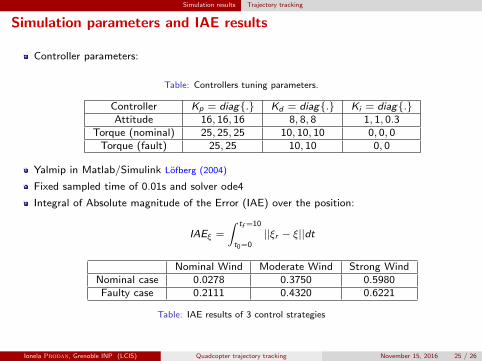
Simulation parameters and IAE results

Controller parameters:

Table: Controllers tuning parameters.

Controller Kp = diag{.} Kd = diag{.} Ki = diag{.}Attitude 16, 16, 16 8, 8, 8 1, 1, 0.3

Torque (nominal) 25, 25, 25 10, 10, 10 0, 0, 0Torque (fault) 25, 25 10, 10 0, 0

Yalmip in Matlab/Simulink Lofberg (2004)

Fixed sampled time of 0.01s and solver ode4

Integral of Absolute magnitude of the Error (IAE) over the position:

IAEξ =

∫ tf =10

t0=0||ξr − ξ||dt

Nominal Wind Moderate Wind Strong WindNominal case 0.0278 0.3750 0.5980Faulty case 0.2111 0.4320 0.6221

Table: IAE results of 3 control strategies


Outline







Conclusions and future developments

Conclusions and future developments

Conclusions:

Quadcopter modeling using Newton-Euler formalism

Novel flat output representation

Trajectory generation problem

Feedback linearization based control designs for trajectory tracking

Robustness under bounded wind perturbations

Control reconfiguration analysis under stuck rotor fault

Extensive simulations for different wind conditions

Future development:

MPC/NMPC implementations

Bounded/stochastic disturbances considerations

Trajectory reconfiguration mechanisms

Experiments on the Crazyflie platform

0Prodan I., Stoican F., Olaru S. and Niculescu S-I. (2016): Mixed-Integer Representations in Control Design, SpringerBriefs inControl, Automation and Robotics Series, Springer.


References IA. Chamseddine, Y. Zhang, C.A. Rabbath, C. Join, and D. Theilliol. Flatness-based trajectory planning/replanning for a quadrotor unmanned aerial vehicle.

IEEE Transactions on Aerospace and Electronic Systems, 48(4):2832–2848, 2012.

J.J. Craig. Introduction to robotics: mechanics and control, volume 3. Pearson Prentice Hall Upper Saddle River, 2005.

J. De Dona, F. Suryawan, M. Seron, and J. Levine. A flatness-based iterative method for reference trajectory generation in constrained NMPC. Int.Workshop on Assesment and Future Direction of Nonlinear Model Predictive Control, pages 325–333, 2009.

M. Fliess, J. Levine, P. Martin, and P. Rouchon. Flatness and defect of non-linear systems: introductory theory and examples. International journal ofcontrol, 61(6):1327–1361, 1995.

Simone Formentin and Marco Lovera. Flatness-based control of a quadrotor helicopter via feedforward linearization. In CDC-ECE, pages 6171–6176, 2011.

J. Levine. Analysis and control of nonlinear systems: A flatness-based approach. Springer Verlag, 2009.

J. Lofberg. Yalmip : A toolbox for modeling and optimization in MATLAB. In Proceedings of the CACSD Conference, Taipei, Taiwan, 2004. URLhttp://users.isy.liu.se/johanl/yalmip.

I. Prodan. Control of Multi-Agent Dynamical Systems in the Presence of Constraints. PhD thesis, Supelec, 2012.

I. Prodan, F. Stoican, S. Olaru, and Niculescu S.I. Enhancements on the Hyperplanes Arrangements in Mixed-Integer Techniques. Journal of OptimizationTheory and Applications, 154(2):549–572, 2012a. doi: 10.1007/s10957-012-0022-9.

I. Prodan, F. Stoican, S. Olaru, C. Stoica, and S-I. Niculescu. Mixed-integer programming techniques in distributed mpc problems. In Distributed MPCmade easy, number 69, pages 273–288. Springer, 2012b.

I. Prodan, S. Olaru, R. Bencatel, J. Sousa, C. Stoica, and S.I. Niculescu. Receding horizon flight control for trajectory tracking of autonomous aerialvehicles. Control Engineering Practice, 21(10):1334–1349, 2013a. doi: 10.1016/j.conengprac.2013.05.010.

I. Prodan, S. Olaru, C. Stoica, and S.I. Niculescu. Predictive control for trajectory tracking and decentralized navigation of multi-agent formations.International Journal of Applied Mathematics and Computer Science, 23(1):91–102, 2013b. doi: 10.2478/amcs-2013-0008.

I. Prodan, S. Olaru, F. Fontes, F. Pereira, C. Stoica Maniu, and S.-I. Niculescu. Predictive control for path following. from trajectory generation to theparametrization of the discrete tracking sequences. In Topics in optimization based control and estimation, pages 161–181. Springer, 2015.

Xin Qi, Didier Theilliol, Juntong Qi, Youmin Zhang, and Jianda Han. A literature review on fault diagnosis methods for manned and unmanned helicopters.In Unmanned Aircraft Systems (ICUAS), 2013 International Conference on, pages 1114–1118. IEEE, 2013.

H. Sira-Ramırez and S. Agrawal. Differential Flatness. Marcel Dekker, New York, 2004.

Z. S. Spakovszky. Unified: Thermodynamics and propulsion, 2007. http://web.mit.edu/16.unified/www/FALL/thermodynamics/notes/notes.html.

F. Stoican, I. Prodan, and D. Popescu. Flat trajectory generation for way-points relaxations and obstacle avoidance. In Proceedings of the 23th IEEEMediterranean Conference on Control and Automation, pages 695–700. IEEE, 2015.

Florin Stoican, Vlad-Mihai Ivanusca, Ionela Prodan, and Dan Popescu. Obstacle avoidance via b-spline parameterizations of flat trajectories. In Proceedingsof the 24th Mediterranean Conference on Control and Automation, pages 1002–1007, Athens, Greece, 2016.

F. Suryawan. Constrained Trajectory Generation and Fault Tolerant Control Based on Differential Flatness and B-splines. PhD thesis, 2012.

F. Suryawan, J. De Dona, and M. Seron. Minimum-time trajectory generation for constrained linear systems using flatness and b-splines. InternationalJournal of Control, 84(9):1565–1585, 2011.

Nitin Sydney, Brendan Smyth, and Derek A Paley. Dynamic control of autonomous quadrotor flight in an estimated wind field. In Decision and Control(CDC), 2013 IEEE 52nd Annual Conference on, pages 3609–3616. IEEE, 2013.

http://users.isy.liu.se/johanl/yalmip

Flatness-based nonlinear control strategies for trajectory ...

Documents

Transcript of Flatness-based nonlinear control strategies for trajectory ...