Fixed Points of Averages of Resolvents:Geometry and Algorithms

Heinz H. Bauschke∗, Xianfu Wang†, and Calvin J.S. Wylie‡

September 27, 2011 revision 2 (original: February 7; revision 1: August 29)

Abstract

To provide generalized solutions if a given problem admits no actual solution is animportant task in mathematics and the natural sciences. It has a rich history datingback to the early 19th century when Carl Friedrich Gauss developed the method ofleast squares of a system of linear equations — its solutions can be viewed as fixedpoints of averaged projections onto hyperplanes. A powerful generalization of thisproblem is to find fixed points of averaged resolvents (i.e., firmly nonexpansive map-pings).

This paper concerns the relationship between the set of fixed points of averagedresolvents and certain fixed point sets of compositions of resolvents. It partially ex-tends recent work for two mappings on a question of C. Byrne. The analysis suggestsa reformulation in a product space. Algorithmic consequences are also presented.

2010 Mathematics Subject Classification: Primary 47H05, 47H09; Secondary 47J25, 65K05, 65K10,90C25.

Keywords: averaged mapping, firmly nonexpansive mapping, fixed point, Hilbert space, leastsquares solutions, maximal monotone operator, nonexpansive mapping, normal equation, projec-tion, resolvent, resolvent average.

∗Mathematics, University of British Columbia, Kelowna, B.C. V1V 1V7, Canada. E-mail:heinz.bauschke@ubc.ca.

†Mathematics, University of British Columbia, Kelowna, B.C. V1V 1V7, Canada. E-mail:shawn.wang@ubc.ca.

‡Mathematics, University of British Columbia, Kelowna, B.C. V1V 1V7, Canada. E-mail:calvin.wylie@gmail.com.

1

1 Introduction

Throughout this paper,

(1) X is a real Hilbert space with inner product 〈·, ·〉

and induced norm ‖ · ‖. We impose that X 6= {0}. To motivate the results of this paper, letus assume that C1, . . . , Cm are finitely many nonempty closed convex subsets of X, withprojections (nearest point mappings) P1, . . . , Pm. Many problems in mathematics and thephysical sciences can be recast as the convex feasibility problem of finding a point in theintersection C1 ∩ · · · ∩ Cm. However, in applications it may well be that this intersectionis empty. In this case, a powerful and very useful generalization of the intersection is theset of fixed points of the operator

(2) X → X : x 7→ P1x + · · ·+ Pmxm

.

(See, e.g., [17] for applications.) Indeed, these fixed points are precisely the minimizers ofthe convex function

(3) X → R : x 7→m

∑i=1‖x− Pix‖2

and—when each Ci is a suitably described hyperplane—there is a well known connectionto the set of least squares solutions in the sense of linear algebra (see Appendix).

A problem open for a long time is to find precise relationships between the fixed pointsof the operator defined in (2) and the fixed points of the composition Pm ◦ · · · ◦ P2 ◦ P1when the intersection C1 ∩ · · · ∩ Cm is empty. (It is well known that both fixed points setscoincide with C1 ∩ · · · ∩Cm provided this intersection is nonempty.) This problem was re-cently explicitly stated and nicely discussed in [14, Chapter 50] and [15, Open Question 2on page 101 in Subsection 8.3.2]. For other related work1, see [3], [5], [16], [19], and thereferences therein. When m = 2, the recent work [34] contains some precise relationships.For instance, the results in [34, Section 3] show that

(4) Fix(P2 ◦ P1)→ Fix(1

2 P1 +12 P2)

: x 7→ 12 x + 1

2 P1x

is a well defined bijection.

1In passing, we mention that when C1, C2, C3 are line segments forming a triangle in the Euclidean plane,then the minimizer of (3) is known as the symmedian point (also known as the Grebe-Lemoine point) ofthe given triangle; see [24, Theorem 349 on page 216].

2

Our goal in this paper is two-fold. First, we wish to find a suitable extension to describe thesefixed point sets when m ≥ 3. Second, we build on these insights to obtain algorithms for findingthese fixed points.

The results provided are somewhat surprising. While we completely generalize someof the two-set work from [34], the generalized intersection is not formulated as the fixedpoint set of a simple composition, but rather as the fixed point set of a more compli-cated operator described in a product space. Nonetheless, the geometric insight obtainedwill turn out to be quite useful in the design of new algorithms that show better conver-gence properties when compared to straight iteration of the averaged projection operator.Furthermore, the results actually hold for very general firmly nonexpansive operators—equivalently, resolvents of maximally monotone operators—although the optimization-based interpretation as a set of minimizers analogous to (3) is then unavailable.

The paper is organized as follows. In the remainder of this introductory section, wedescribe some central notions fundamental to our analysis. The main result of Section 2is Theorem 2.1 where we provide a precise correspondence between the fixed point set ofan averged resolvent JA and a certain set S in a product space. In Section 3, it is shownthat S is in fact the fixed point set of an averaged mapping (see Corollary 3.8). This insightis brought to good use in Section 4, where we design a new algorithm for finding a pointin S (and hence in Fix JA) and where we provide a rigorous convergence proof. Akin tothe Gauss-Seidel variant of the Jacobi iteration in numerical linear algebra, we proposeanother new algorithm. An appendix connecting fixed points of averages of projectionsonto hyperplanes to classical least squares solutions concludes the paper. The notationwe utilize is standard and as in [4], [8], [29], [30], [32], [33], or [35] to which we also referfor background.

Recall that a mapping

(5) T : X → X

is firmly nonexpansive (see [36] for the first systematic study) if

(6) (∀x ∈ X)(∀y ∈ X) ‖Tx− Ty‖2 + ‖(Id−T)x− (Id−T)y‖2 ≤ ‖x− y‖2,

where Id : X → X : x 7→ x denotes the identity operator. The prime examples of firmlynonexpansive mappings are projection operators (also known as nearest point map-pings) with respect to nonemtpy closed convex subsets of X. It is clear that if T is firmlynonexpansive, then it is nonexpansive, i.e., Lipschitz continuous with constant 1,

(7) (∀x ∈ X)(∀y ∈ X) ‖Tx− Ty‖ ≤ ‖x− y‖;

the converse, however, is false (consider − Id). The set of fixed points of T is

(8) Fix T ={

x ∈ X∣∣ x = Tx

}.

3

The following characterization of firm nonexpansiveness is well known and will beused repeatedly.

Fact 1.1 (See, e.g., [4, 21, 22].) Let T : X → X. Then the following are equivalent:

(i) T is firmly nonexpansive.

(ii) Id−T is firmly nonexpansive.

(iii) 2T − Id is nonexpansive.

(iv) (∀x ∈ X)(∀y ∈ X) ‖Tx− Ty‖2 ≤ 〈x− y, Tx− Ty〉.

(v) (∀x ∈ X)(∀y ∈ X) 0 ≤ 〈Tx− Ty, (Id−T)x− (Id−T)y〉.

Firmly nonexpansive mappings are also intimately tied with maximally monotone op-erators. Recall that a set-valued operator A : X ⇒ X (i.e., (∀x ∈ X) Ax ⊆ X) with graphgr A is monotone if

(9) (∀(x, u) ∈ gr A)(∀(y, v) ∈ gr A) 〈x− y, u− v〉 ≥ 0,

and that A is maximally monotone if it is monotone and every proper extension of A failsto be monotone. We write dom A =

{x ∈ X

∣∣ Ax 6= ∅}

and ran A = A(X) =⋃

x∈X Axfor the domain and range of A, respectively. The inverse of A is defined via gr A−1 ={(u, x) ∈ X× X

∣∣ u ∈ Ax}

. Monotone operators are ubiquitous in modern analysis andoptimization; see, e.g., the books [4], [8], [9], [13], [32], [33], [35], [37], [38], and [39].Two key examples of maximally monotone operators are continuous linear monotoneoperators and subdifferential operators (in the sense of convex analysis) of functions thatare convex, lower semicontinuous, and proper.

Now let A : X ⇒ X be maximally monotone and denote the associated resolvent by

(10) JA = (Id+A)−1.

In [27], Minty made the seminal observation that JA is in fact a firmly nonexpansive op-erator from X to X and that, conversely, every firmly nonexpansive operator arises thisway:

Fact 1.2 (Minty) (See, e.g., [27] or [20].) Let T : X → X be firmly nonexpansive, and letA : X ⇒ X be maximally monotone. Then the following hold.

(i) B = T−1 − Id is maximally monotone (and JB = T).

(ii) JA is firmly nonexpansive (and A = J−1A − Id).

4

One of the motivations to study the correspondence between firmly nonexpansivemappings and maximally monotone operators is the very useful correspondence

(11) A−1(0) = Fix JA,

where A : X ⇒ X is maximally monotone.

From now on we assume that

(12) A1, . . . , Am are maximally monotone operators on X, where m ∈ {2, 3, . . .},

that

(13) λ1, . . . , λm belong to ]0, 1[ such that ∑i∈I

λi = 1, where I = {1, 2, . . . , m},

and we set

(14) A =

(∑i∈I

λi JAi

)−1

− Id .

Then the definition of the resolvent yields

(15) JA = ∑i∈I

λi JAi ;

thus, since it is easy to see that JA is firmly nonexpansive, it follows from Fact 1.2 thatA is maximally monotone. We refer to the operator A as the resolvent average of themaximally monotone operators A1, . . . , Am and we note that JA is the weighted averageof the resolvents JAi . The operator JA is the announced generalization of the averagedprojection operator considered in (2), and Fix JA is the generalization of the minimizers ofthe function in (3). For a related discussion, see also [18, Section 6.3].

This introductory section is now complete. In the next section, we shall derive an alter-native description of Fix JA.

5

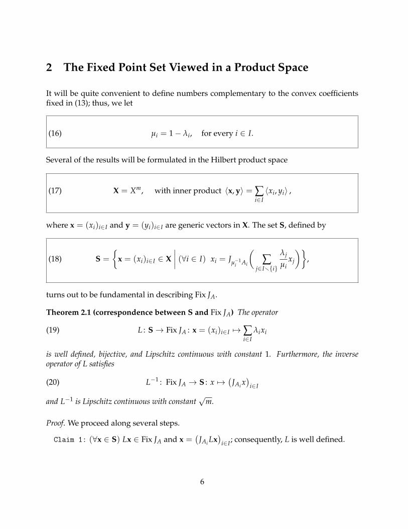
2 The Fixed Point Set Viewed in a Product Space

It will be quite convenient to define numbers complementary to the convex coefficientsfixed in (13); thus, we let

(16) µi = 1− λi, for every i ∈ I.

Several of the results will be formulated in the Hilbert product space

(17) X = Xm, with inner product 〈x, y〉 = ∑i∈I〈xi, yi〉 ,

where x = (xi)i∈I and y = (yi)i∈I are generic vectors in X. The set S, defined by

(18) S =

{x = (xi)i∈I ∈ X

∣∣∣∣ (∀i ∈ I) xi = Jµ−1i Ai

(∑

j∈Ir{i}

λj

µixj

)},

turns out to be fundamental in describing Fix JA.

Theorem 2.1 (correspondence between S and Fix JA) The operator

(19) L : S→ Fix JA : x = (xi)i∈I 7→∑i∈I

λixi

is well defined, bijective, and Lipschitz continuous with constant 1. Furthermore, the inverseoperator of L satisfies

(20) L−1 : Fix JA → S : x 7→(

JAi x)

i∈I

and L−1 is Lipschitz continuous with constant√

m.

Proof. We proceed along several steps.

Claim 1: (∀x ∈ S) Lx ∈ Fix JA and x =(

JAi Lx)

i∈I ; consequently, L is well defined.

6

Let x = (xi)i∈I ∈ S and set x = ∑i∈I λixi = Lx. Using the definition of the resolvent,we have, for every i ∈ I,

∑j∈Ir{i}

λj

µixj ∈

(Id+µ−1

i Ai)xi ⇔ ∑

j∈Ir{i}λjxj ∈ µixi + Aixi(21a)

⇔ ∑j∈Ir{i}

λjxj ∈ (1− λi)xi + Aixi(21b)

⇔ x = ∑j∈I

λjxj ∈(

Id+Ai)xi(21c)

⇔ xi = JAi x = JAi Lx.(21d)

Hence x =(

JAi Lx)

i∈I , as claimed. Moreover, (∀i ∈ I) λixi = λi JAi x, which, after sum-ming over i ∈ I and recalling (15), yields x = ∑i∈I λixi = ∑i∈I λi JAi x = JA x. ThusLx = x ∈ Fix JA and Claim 1 is verified.

Claim 2: (∀x ∈ Fix JA)(

JAi x)

i∈I ∈ S.Assume that x ∈ Fix JA and set (∀i ∈ I) yi = JAi x. Then, using (15), we see that

(22) ∑i∈I

λiyi = ∑i∈I

λi JAi x = JAx = x.

Furthermore, for every i ∈ I, and using (22) in the derivation of (23c)

yi = JAi x ⇔ x ∈ yi + Aiyi ⇔ x− λiyi ∈ µiyi + Aiyi(23a)

⇔ µ−1i(

x− λiyi)∈(

Id+µ−1i Ai

)yi(23b)

⇔ µ−1i ∑

j∈Ir{i}λjyj ∈

(Id+µ−1

i Ai

)yi(23c)

⇔ yi = Jµ−1i Ai

(∑

j∈Ir{i}

λj

µiyj

).(23d)

Thus, (yi)i∈I ∈ S and Claim 2 is verified.

Having verified the two claims above, we now turn to proving the statements an-nounced.

First, let x ∈ Fix JA. By Claim 2, (JAi x)i∈I ∈ S. Hence L(JAi x)i∈I = ∑i∈I λi JAi x = JAx =x by (15). Thus, L is surjective.

Second, assume that x = (xi)i∈I and y = (yi)i∈I belong to S and that Lx = Ly. Then,using Claim 1, we see that x = (JAi Lx)i∈I = (JAi Ly)i∈I = y and thus L is injective.Altogether, this shows that L is bijective and we also obtain the formula for L−1.

7

Third, again let x = (xi)i∈I and y = (yi)i∈I be in S. Using the convexity of ‖ · ‖2, weobtain

‖Lx− Ly‖2 =∥∥∥∑

i∈Iλi(xi − yi)

∥∥∥2≤∑

i∈Iλi‖xi − yi‖2(24a)

≤∑i∈I‖xi − yi‖2 = ‖x− y‖2.(24b)

Thus, L is Lipschitz continuous with constant 1.

Finally, let x and y be in Fix JA. Since JAi is (firmly) nonexpansive for all i ∈ I, weestimate ∥∥L−1x− L−1y

∥∥2=∥∥∥(JAi x

)i∈I −

(JAi y

)i∈I

∥∥∥2= ∑

i∈I

∥∥JAi x− JAi y∥∥2(25a)

≤∑i∈I‖x− y‖2 = m‖x− y‖2.(25b)

Therefore, L−1 is Lipschitz continuous with constant√

m. �

Remark 2.2 Some comments regarding Theorem 2.1 are in order.

(i) Because of the simplicity of the bijection L provided in Theorem 2.1, the task offinding Fix JA is essentially the same as finding S.

(ii) Note that when each Ai is a normal cone operator NCi , then the resolvents JAi andJµ−1

i Aisimplify to the projections PCi , for every i ∈ I.

(iii) When m = 2, the set S turns into

(26) S ={(x1, x2) ∈ X

∣∣ x1 = Jλ−12 A1

x2 and x2 = Jλ−11 A2

x1}

,

and Theorem 2.1 coincides with [34, Theorem 3.6]. Note that (x1, x2) ∈ S if and onlyif x2 ∈ Fix

(Jλ−1

1 A2Jλ−1

2 A1

)and x1 = Jλ−1

2 A1x2, which makes the connection between

the fixed point set of the composition of the two resolvents and S. It appears thatthis is a particularity of the case m = 2; it seems that there is no simple connectionbetween fixed points of Jµ−1

m AmJµ−1

m−1 Am−1· · · Jµ−1

1 A1and Fix JA when m ≥ 3.

8

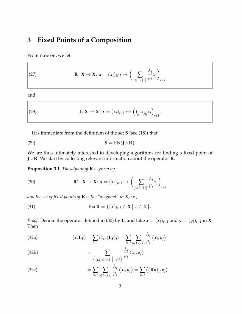
3 Fixed Points of a Composition

From now on, we let

(27) R : X→ X : x = (xi)i∈I 7→(

∑j∈Ir{i}

λj

µixj

)i∈I

and

(28) J : X→ X : x = (xi)i∈I 7→(

Jµ−1i Ai

xi

)i∈I

.

It is immediate from the definition of the set S (see (18)) that

(29) S = Fix(J ◦ R).

We are thus ultimately interested in developing algorithms for finding a fixed point ofJ ◦ R. We start by collecting relevant information about the operator R.

Proposition 3.1 The adjoint of R is given by

(30) R∗ : X→ X : x = (xi)i∈I 7→(

∑j∈Ir{i}

λi

µjxj

)i∈I

and the set of fixed points of R is the “diagonal” in X, i.e.,

(31) Fix R ={(x)i∈I ∈ X

∣∣ x ∈ X}

.

Proof. Denote the operator defined in (30) by L, and take x = (xi)i∈I and y = (yi)i∈I in X.Then

〈x, Ly〉 = ∑i∈I〈xi, (Ly)i〉 = ∑

i∈I∑

j∈Ir{i}

λi

µj

⟨xi, yj

⟩(32a)

= ∑{(i,j)∈I×I

∣∣ i 6=j} λi

µj

⟨xi, yj

⟩(32b)

= ∑j∈I

∑i∈Ir{j}

λi

µj

⟨xi, yj

⟩= ∑

j∈I

⟨(Rx)j, yj

⟩(32c)

9

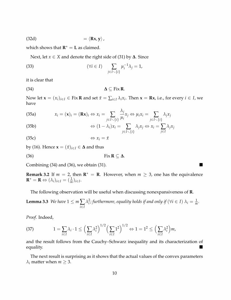
= 〈Rx, y〉 ,(32d)

which shows that R∗ = L as claimed.

Next, let x ∈ X and denote the right side of (31) by ∆. Since

(33) (∀i ∈ I) ∑j∈Ir{i}

µ−1i λj = 1,

it is clear that

(34) ∆ ⊆ Fix R.

Now let x = (xi)i∈I ∈ Fix R and set x = ∑i∈I λixi. Then x = Rx, i.e., for every i ∈ I, wehave

xi = (x)i = (Rx)i ⇔ xi = ∑j∈Ir{i}

λj

µixj ⇔ µixi = ∑

j∈Ir{i}λjxj(35a)

⇔ (1− λi)xi = ∑j∈Ir{i}

λjxj ⇔ xi = ∑j∈I

λjxj(35b)

⇔ xi = x(35c)

by (16). Hence x = (x)i∈I ∈ ∆ and thus

(36) Fix R ⊆ ∆.

Combining (34) and (36), we obtain (31). �

Remark 3.2 If m = 2, then R∗ = R. However, when m ≥ 3, one has the equivalenceR∗ = R⇔ (λi)i∈I = ( 1

m )i∈I .

The following observation will be useful when discussing nonexpansiveness of R.

Lemma 3.3 We have 1 ≤ m ∑i∈I

λ2i ; furthermore, equality holds if and only if (∀i ∈ I) λi =

1m .

Proof. Indeed,

1 = ∑i∈I

λi · 1 ≤(

∑i∈I

λ2i

)1/2(∑i∈I

12)1/2

⇔ 1 = 12 ≤(

∑i∈I

λ2i

)m,(37)

and the result follows from the Cauchy–Schwarz inequality and its characterization ofequality. �

The next result is surprising as it shows that the actual values of the convex parametersλi matter when m ≥ 3.

10

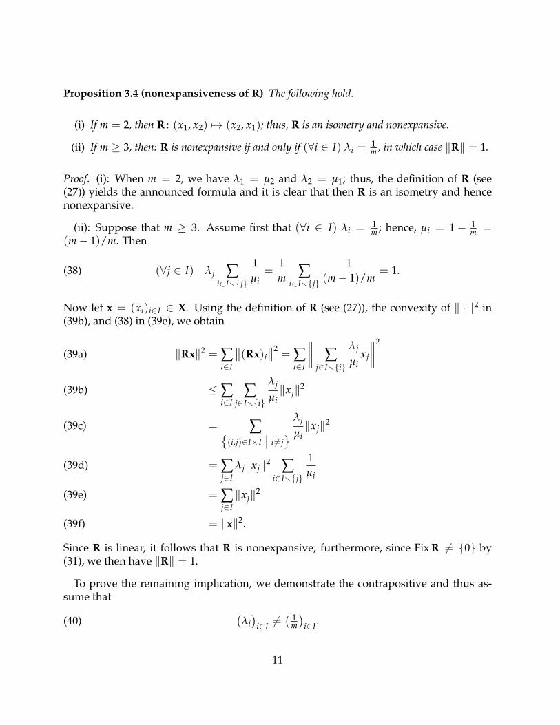
Proposition 3.4 (nonexpansiveness of R) The following hold.

(i) If m = 2, then R : (x1, x2) 7→ (x2, x1); thus, R is an isometry and nonexpansive.

(ii) If m ≥ 3, then: R is nonexpansive if and only if (∀i ∈ I) λi =1m , in which case ‖R‖ = 1.

Proof. (i): When m = 2, we have λ1 = µ2 and λ2 = µ1; thus, the definition of R (see(27)) yields the announced formula and it is clear that then R is an isometry and hencenonexpansive.

(ii): Suppose that m ≥ 3. Assume first that (∀i ∈ I) λi = 1m ; hence, µi = 1− 1

m =(m− 1)/m. Then

(38) (∀j ∈ I) λj ∑i∈Ir{j}

1µi

=1m ∑

i∈Ir{j}

1(m− 1)/m

= 1.

Now let x = (xi)i∈I ∈ X. Using the definition of R (see (27)), the convexity of ‖ · ‖2 in(39b), and (38) in (39e), we obtain

‖Rx‖2 = ∑i∈I

∥∥(Rx)i∥∥2

= ∑i∈I

∥∥∥∥ ∑j∈Ir{i}

λj

µixj

∥∥∥∥2

(39a)

≤∑i∈I

∑j∈Ir{i}

λj

µi‖xj‖2(39b)

= ∑{(i,j)∈I×I

∣∣ i 6=j} λj

µi‖xj‖2(39c)

= ∑j∈I

λj‖xj‖2 ∑i∈Ir{j}

1µi

(39d)

= ∑j∈I‖xj‖2(39e)

= ‖x‖2.(39f)

Since R is linear, it follows that R is nonexpansive; furthermore, since Fix R 6= {0} by(31), we then have ‖R‖ = 1.

To prove the remaining implication, we demonstrate the contrapositive and thus as-sume that

(40)(λi)

i∈I 6=( 1

m)

i∈I .

11

Take u ∈ X such that ‖u‖ = 1 and set (∀i ∈ I) xi = µiu and x = (xi)i∈I . We compute

‖x‖2 = ∑i∈I‖xi‖2 = ∑

i∈I‖µiu‖2 = ∑

i∈Iµ2

i(41a)

= ∑i∈I

(1− λi)2 = ∑

i∈I

(1− 2λi + λ2

i)

(41b)

= m− 2 + ∑i∈I

λ2i .(41c)

Using (30), the fact that ‖u‖ = 1, we obtain

‖R∗x‖2 = ∑i∈I

λ2i

∥∥∥∥ ∑j∈Ir{i}

µ−1j xj

∥∥∥∥2

= ∑i∈I

λ2i

∥∥∥∥ ∑j∈Ir{i}

µ−1j µju

∥∥∥∥2

(42a)

= ∑i∈I

λ2i∥∥(m− 1)u

∥∥2= (m− 1)2 ∑

i∈Iλ2

i(42b)

Altogether,

‖R∗x‖2 − ‖x‖2 = 2−m +((m− 1)2 − 1

)∑i∈I

λ2i(43a)

= (m− 2)(− 1 + m ∑

i∈Iλ2

i

).(43b)

Now m ≥ 3 implies that m − 2 > 0; furthermore, by (40) and Lemma 3.3, −1 +m ∑i∈I λ2

i > 0. Therefore,

(44) ‖R∗x‖ > ‖x‖.

This implies ‖R∗‖ > 1 and hence ‖R‖ > 1 by [25, Theorem 3.9-2]. Since R is linear, itcannot be nonexpansive. �

For algorithmic purposes, nonexpansiveness is a desirable property but it does notguarantee the convergence of the iterates to a fixed point (consider, e.g., − Id). The veryuseful notion of an averaged mapping, which is intermediate between nonexpansivenessand firm nonexpansiveness, was introduced by Baillon, Bruck, and Reich in [2].

Definition 3.5 (averaged mapping) Let T : X → X. Then T is averaged if there exist a non-expansive mapping N : X → X and α ∈ [0, 1[ such that

(45) T = (1− α) Id+αN;

if we wish to emphasis the constant α, we say that T is α-averaged.

12

It is clear from the definition that every averaged mapping is nonexpansive; the con-verse, however, is false: indeed, − Id is nonexpansive, but not averaged. It follows fromFact 1.1 that every firmly nonexpansive mapping is 1

2 -averaged.

The class of averaged mappings is closed under compositions; this is not true for firmlynonexpansive mappings: e.g., consider two projections onto two lines that meet at 0 at aπ/4 angle. Let us record the following well known key properties.

Fact 3.6 Let T, T1, and T2 be mappings from X to X, let α1 and α2 be in [0, 1[, and let x0 ∈ X.Then the following hold.

(i) T is firmly nonexpansive if and only if T is 12 -averaged.

(ii) If T1 is α1-averaged and T2 is α2-averaged, then T1 ◦ T2 is α-averaged, where

(46) α =

0, if α1 = α2 = 0;2

1 + 1/ max{α1, α2}, otherwise

is the harmonic mean of 1 and max{α1, α2}.

(iii) If T1 and T2 are averaged, and Fix(T1 ◦ T2) 6= ∅, then Fix(T1 ◦ T2) = Fix(T1) ∩ Fix(T2).

(iv) If T is averaged and Fix T 6= ∅, then the sequence of iterates (Tnx0)n∈N converges weakly2

to a point in Fix T; otherwise, ‖Tnx0‖ → +∞.

Proof. (i): This is well known and immediate from Fact 1.1.

(ii): The fact that the composition of averaged mappings is again averaged is wellknown and implicit in the proof of [2, Corollary 2.4]. For the exact constants, see [18,Lemma 2.2] or [4, Proposition 4.32].

(iii): This follows from [12, Proposition 1.1, Proposition 2.1, and Lemma 2.1]. See also[28, Theorem 3] for the case when Fix T 6= ∅.

(iv): This follows from [12, Corollary 1.3 and Corollary 1.4]. �

Theorem 3.7 (averagedness of R) The following hold.

(i) If m = 2, then R is not averaged.

(ii) If m ≥ 3 and (∀i ∈ I) λi =1m , then R = (1− α) Id+αN, where α = m

2m−2 and N is anisometry; in particular, R is α-averaged.

2When T is firmly nonexpansive, the weak convergence goes back at least to [11].

13

Proof. (i): Assume that m = 2. By Proposition 3.4(i), R : (x1, x2) 7→ (x2, x1). We argueby contradiction and thus assume that R is averaged, i.e., there exist a nonexpansivemapping N : X → X and α ∈ [0, 1[ such that R = (1− α) Id+αN. Since R 6= Id, it is clearthat α > 0. Thus,

(47) N : X→ X : (x1, x2) 7→ α−1(x2 − x1 + αx1, x1 − x2 + αx2).

Now take u ∈ X such that ‖u‖ = 1 and set x = (x1, x2) = (0, αu). Then

(48) ‖x‖2 = ‖0‖2 + ‖αu‖2 = α2

and Nx =(u, (α− 1)u

). Thus,

(49) ‖Nx‖2 = ‖u‖2 + ‖(α− 1)u‖2 = 1 + (1− α)2 = α2 + 2(1− α) > α2 = ‖x‖2.

Hence ‖N‖ > 1 and, since N is linear, N cannot be nonexpansive. This contradictioncompletes the proof of (i).

(ii): Assume that m ≥ 3 and that (∀i ∈ I) λi =1m . For future reference, we observe that

(50) (∀i ∈ I)(∀j ∈ I)λj

µi=

1m

1− 1m

=1

m− 1.

We start by defining

(51) L : X→ X : (xi)i∈I 7→∑i∈I

xi.

Then it is easily verified that

(52) L∗ : X → X : x 7→ (x)i∈I

and hence that

(53) L∗LL∗L = mL∗L.

Now set

(54) α =m

2m− 2and N = α−1(R− (1− α) Id

).

Then α ∈ ]0, 1[ and R = αN + (1− α) Id; thus, it suffices to show that N is an isometry.Note that

(55) α− 1 = −α +1

m− 1.

14

Take x = (xi)i∈I ∈ X. Using (27), (50), and (55), we obtain for every i ∈ I,

(Nx)i = α−1(− (1− α)xi + (Rx)i)

(56a)

= α−1((α− 1)xi + ∑

j∈Ir{i}

λj

µixj

)(56b)

= α−1(− αxi +

1m− 1

xi + ∑j∈Ir{i}

1m− 1

xj

)(56c)

= α−1(− αxi + ∑

j∈I

1m− 1

xj

)(56d)

= −xi +α−1

m− 1Lx(56e)

= −xi +2m

Lx;(56f)

hence, Nx = −x + 2m L∗Lx. It follows that N = − Id+ 2

m L∗L and thus N∗ = N. Using (53),we now obtain

N∗N = NN =(− Id+ 2

m L∗L)(− Id+ 2

m L∗L)

(57a)

= Id− 2m L∗L− 2

m L∗L + 4m2

(L∗LL∗L

)(57b)

= Id− 4m L∗L + 4

m2

(mL∗L

)(57c)

= Id .(57d)

Therefore, ‖Nx‖2 = 〈Nx, Nx〉 = 〈x, N∗Nx〉 = 〈x, x〉 = ‖x‖2 and hence N is an isometry;in particular, N is nonexpansive and R is α-averaged. �

We are now in a position to describe the set S as the fixed point set of an averagedmapping.

Corollary 3.8 Suppose that m ≥ 3 and that (∀i ∈ I) λi =1m . Then J ◦ R is 2m

3m−2 -averaged andFix(J ◦ R) = S.

Proof. On the one hand, since J is clearly firmly nonexpansive, J is 12 -averaged. On the

other hand, by Theorem 3.7(ii), R is m2m−2 -averaged. Since 0 < 1

2 < m2m−2 , it follows from

Fact 3.6(ii) that J ◦ R is α-averaged, where

(58) α =2

1 + 1/(m/(2m− 2))=

2m3m− 2

,

as claimed. To complete the proof, recall (29). �

15

4 Algorithmic Consequences

In Section 2, we saw that Fix JA = L(S) (see Theorem 2.1), and in Section 3 we discoveredthat S = Fix(J ◦ R) is the fixed point set of an averaged operator. This analysis leads tonew algorithms for finding a point in Fix JA.

Theorem 4.1 Suppose that m ≥ 3 and that (∀i ∈ I) λi = 1m . Let x0 = (x0,i)i∈I ∈ X and

generate the sequence (xn)n∈N by

(59) (∀n ∈N) xn+1 = (J ◦ R)xn.

Then exactly one of the following holds.

(i) Fix JA 6= ∅, (xn)n∈N converges weakly to a point x = (xi)i∈I in S and (∑i∈I λixn,i)n∈N

converges weakly to ∑i∈I λixi ∈ Fix JA.

(ii) Fix JA = ∅ and ‖xn‖ → +∞.

Proof. By Theorem 2.1, S 6= ∅ if and only if Fix JA 6= ∅. Furthermore, Corollary 3.8 showsthat S = Fix(J ◦ R), where J ◦ R is averaged. The result thus follows from Fact 3.6(iv),Theorem 2.1, and the weak continuity of the operator L defined in (19). �

Remark 4.2 The assumption that m ≥ 3 in Theorem 4.1 is critical: indeed, suppose thatm = 2. Then, by Proposition 3.4(i), R : (x1, x2) 7→ (x2, x1). Now assume further thatA1 = A2 ≡ 0. Then J = Id and hence J ◦ R = R. Thus, if y and z are two distinctpoints in X and the sequence (xn)n∈N is generated by iterating J ◦R with a starting pointx0 = (y, z), then

(60) (∀n ∈N) xn =

{(y, z), if n is even;(z, y), if n is odd.

Consequently, (xn)n∈N is a bounded sequence that is not weakly convergent. On theother hand, keeping the assumption m = 2 but allowing again for general maximallymonotone operators A1 and A2, and assuming that Fix JA 6= ∅, we observe that

(61) J ◦ R ◦ J ◦ R : X→ X : (x1, x2) 7→(

Jλ−12 A1

Jλ−11 A2

x1, Jλ−11 A2

Jλ−12 A1

x2).

Hence, by [34, Theorem 5.3], the even iterates of J ◦R will converge weakly to point (x1, x2)with x1 = Jλ−1

2 A1Jλ−1

1 A2x1 and x2 = Jλ−1

1 A2Jλ−1

2 A1x2. However, (x1, x2) /∈ S in general.

We are grateful to a referee for pointing out that —in the context of proximityoperators— the algorithm presented in Theorem 4.1 is a special case of an algorithm de-veloped in [10, Section 5.3]. While the results in [10] are given for proximity operators, anextension to resolvents is possible by reasoning as in [1].

16

Remark 4.3 Just as the Gauss-Seidel iteration can be viewed as a modification of the Ja-cobi iteration where new information is immediately utilized (see, e.g., [23, Chapters 4and 5] and [31, Section 4.1]), we similarly modify the iteration of the operator J ◦ R. Tothis end, we introduce, for every k ∈ I, the following operators from X to X:

(62)(∀x = (xi)i∈I ∈ X

)(∀i ∈ I) (Rkx)i =

xi, if i 6= k;

∑j∈Ir{k}

λj

µkxj, if i = k,

and

(63)(∀x = (xi)i∈I ∈ X

)(∀i ∈ I) (Jkx)i =

xi, if i 6= k;

Jµ−1k Ak

xk, if i = k.

It follows from the definition of S (see (18)) that S =⋂

k∈I Fix(Jk ◦ Rk). This implies

(64) S ⊆ Fix(Jm ◦ Rm ◦ · · · ◦ J1 ◦ R1

),

and it motivates—but does not justify—to iterate the composition

(65) T = Jm ◦ Rm ◦ · · · ◦ J1 ◦ R1

in order to find points in S. In general, the composition T is not nonexpansive evenwhen (∀k ∈ I) Ak ≡ 0 so that Jk = Id. Then T = Rm ◦ · · · ◦ R1 and this compositionis not nonexpansive and neither is any Rk (see [6, Proof of Remark 4.3 in Appendix B]).One may verify that Jk ◦ Rk is Lipschitz continuous with constant

√m/(m− 1) when(

λi)

i∈I =( 1

m)

i∈I (see [6, Proof of Remark 4.4 in Appendix B]). In turn, this implies that Tis Lipschitz continuous with constants (m/(m− 1))m/2. Using elementary calculus, oneverifies that when m → +∞, the Lipschitz constant of T decreases to

√exp(1) ≈ 1.6487.

Numerical experiments (which are explained in more detail in [6, Section 4]) show thatiterating T is faster than iterating JA and J ◦ R, which perform quite similarly. Let usnow list some open problems. Suppose that m ≥ 3. We do not know the answers to thefollowing questions.

Q1: Concerning (64), is it actually true that S = Fix T?

Q2: Can one give simple sufficient or necessary conditions for the convergence of theheuristic algorithm, i.e., the iteration of T, when Fix T 6= ∅?

Q3: Under the most general assumption (13), we observed convergence in numericalexperiments of the new rigorous algorithm even though there is no underlyingtheory—see Proposition 3.4(ii) and Theorem 4.1. Can one provide simple sufficientor necessary conditions for the convergence of the sequence defined by (59)?

17

Finally, Q1 and Q2 have affirmative answers when m = 2: indeed, one then computes

(66) T : X→ X : (x1, x2) 7→(

Jλ−12 A1

x2, Jλ−11 A2

Jλ−12 A1

x2

)and hence (x1, x2) ∈ Fix T if and only if x1 = Jλ−1

2 A1x2 and x2 = Jλ−1

1 A2x1, which is the

same as requiring that (x1, x2) ∈ S. When S = Fix T 6= ∅, then the iterates of T convergeweakly to a fixed point by [34, Theorem 5.3(i)].

Appendix

Most of this part of the appendix is part of the folklore; however, we include it here forcompleteness and because we have not quite found a reference that makes all points wewish to stress.

We assume that m ∈ {1, 2, . . .}, that I = {1, 2, . . . , m} and that (Ci)i∈I is a family ofclosed hyperplanes given by

(67) (∀i ∈ I) Ci ={

x ∈ X∣∣ 〈ai, x〉 = bi

}, where ai ∈ X r {0} and bi ∈ R,

with corresponding projections Pi. Set A : X → Rm : x 7→ (〈ai, x〉)i∈I and b = (bi)i∈I ∈Rm. Then A∗ : Rm → X : (yi)i∈I 7→ ∑i∈I yiai. Denote, for every i ∈ I, the ith unit vector inRm by ei, and the projection Rm → Rm : y 7→ 〈y, ei〉 ei onto R ei by Qi. Note that

(68) ∑i∈I

Qi = Id and (∀(i, j) ∈ I × I) QiQj =

{Qi, if i = j;0, otherwise.

We now assume that

(69) (∀i ∈ I) ‖ai‖ = 1,

which gives rise to the pleasant representation of the projectors as

(70) (∀i ∈ I) Pi : x 7→ x− A∗Qi(Ax− b)

and to (see (3))

(71) (∀x ∈ X) ‖Ax− b‖2 = ∑i∈I

∣∣ 〈ai, x〉 − bi∣∣2 = ∑

i∈I

∥∥x− Pix∥∥2.

Now let x ∈ X. Using (70) and (68), we thus obtain the following characterization of fixedpoints of averaged projections:

x ∈ Fix(

∑i∈I

λiPi

)(72a)

18

⇔ x = ∑i∈I

λiPix(72b)

⇔ x = ∑i∈I

λi(x− A∗Qi(Ax− b)

)(72c)

⇔ x =(

∑i∈I

λix)− A∗∑

i∈IλiQi(Ax− b)(72d)

⇔ A∗(

∑i∈I

λiQi

)(Ax− b) = 0(72e)

⇔ A∗(

∑i∈I

√λiQi

)(∑i∈I

√λiQi

)(Ax− b) = 0(72f)

⇔ A∗(

∑i∈I

√λiQi

)(∑i∈I

√λiQi

)Ax = A∗

(∑i∈I

√λiQi

)(∑i∈I

√λiQi

)b(72g)

⇔((

∑i∈I

√λiQi

)A)∗((

∑i∈I

√λiQi

)A)

x =

((∑i∈I

√λiQi

)A)∗(

∑i∈I

√λiQi

)b(72h)

⇔ x satisfies the normal equation of the system(72i) ((∑i∈I

√λiQi

)A)

x =(

∑i∈I

√λiQi

)b(72j)

⇔((

∑i∈I

√mλiQi

)A)∗((

∑i∈I

√mλiQi

)A)

x(72k)

=

((∑i∈I

√mλiQi

)A)∗(

∑i∈I

√mλiQi

)b(72l)

⇔ x satisfies the normal equation of the system(72m) ((∑i∈I

√mλiQi

)A)

x =(

∑i∈I

√mλiQi

)b.(72n)

Note that when (λi)i∈I = ( 1m )i∈I , i.e., we have equal weights, then (72) and (68) yield

x ∈ Fix(

1m ∑

i∈IPi

)⇔((

∑i∈I

Qi

)A)∗((

∑i∈I

Qi

)A)

x =

((∑i∈I

Qi

)A)∗(

∑i∈I

Qi

)b(73a)

⇔ A∗Ax = A∗b(73b)⇔ x satisfies the normal equation of the system Ax = b(73c)⇔ x is a least squares solution of the system Ax = b.(73d)

In other words, the fixed points of the equally averaged projections onto hyperplanes are preciselythe classical least squares solutions encountered in linear algebra, i.e., the solutions to the classi-cal normal equation A∗Ax = A∗b of the system Ax = b. The idea of least squares solutionsgoes back to the famous prediction of the asteroid Ceres due to Carl Friedrich Gauss in1801 (see [7, Subsection 1.1.1] and also [26, Epilogue in Section 4.6]).

19

Example. Consider the following inconsistent linear system of equations

x = 1(74a)x = 2,(74b)

which was also studied by Byrne [15, Subsection 8.3.2 on page 100]. Here m = 2 and (69)holds, and the above discussion yields that Fix

(12 P1 +

12 P2)

and the set of least squaressolutions coincide, namely with the singleton

{32

}. Now change the representation to

2x = 2(75a)x = 2,(75b)

so that (69) is violated. The set of fixed points remains unaltered as the two hyperplanesC1 and C2 are unchanged and thus it equals

{32

}. However, the set of least squares so-

lutions is now{6

5

}. Similarly and returning to the first representation in (74), the set of

fixed points will changes if we consider different weights, say λ1 = 13 and λ2 = 2

3 : indeed,we then obtain Fix

(13 P1 +

23 P2)={5

3

}while the set of least squares solutions is still

{32

}.

Acknowledgments

The authors thank the referees for their thoughtful and constructive comments, and forbringing [1], [10], and [23] to our attention. Heinz Bauschke was partially supported bythe Natural Sciences and Engineering Research Council of Canada and by the CanadaResearch Chair Program. Xianfu Wang was partially supported by the Natural Sciencesand Engineering Research Council of Canada. Calvin Wylie was partially supported bythe Irving K. Barber Endowment Fund.

References

[1] H. Attouch, L.M. Briceno-Arias, and P.L. Combettes, A parallel splitting method for coupledmonotone inclusions, SIAM Journal on Control and Optimization 48 (2010), 3246–3270.

[2] J.B. Baillon, R.E. Bruck, and S. Reich, On the asymptotic behavior of nonexpansive mappingsand semigroups in Banach spaces, Houston Journal of Mathematics 4 (1978), 1–9.

[3] H.H. Bauschke, J.M. Borwein, and A.S. Lewis, The method of cyclic projections for closedconvex sets in Hilbert space, in Recent Developments in Optimization Theory and Nonlin-ear Analysis (Jerusalem 1995), Y. Censor and S. Reich (editors), Contemporary Mathemat-ics vol. 204, American Mathematical Society, pp. 1–38, 1997.

20

[4] H.H. Bauschke and P.L. Combettes, Convex Analysis and Monotone Operator Theory in HilbertSpaces, Springer-Verlag, 2011.

[5] H.H. Bauschke and M.R. Edwards, A conjecture by De Pierro is true for translates of regularsubspaces, Journal of Nonlinear and Convex Analysis 6 (2005), 93–116.

[6] H.H. Bauschke, X. Wang, and C.J.S. Wylie, Fixed points of averages of resolvents: geometryand algorithms, http://arxiv.org/pdf/1102.1478v1, February 2011.

[7] A. Bjorck, Numerical Methods for Least Squares Problems, SIAM, 1996.

[8] J.M. Borwein and J.D. Vanderwerff, Convex Functions, Cambridge University Press, 2010.

[9] H. Brezis, Operateurs Maximaux Monotones et Semi-Groupes de Contractions dans les Espaces deHilbert, North-Holland/Elsevier, 1973.

[10] L.M. Briceno-Arias and P.L. Combettes, Convex variational formulation with smooth cou-pling for multicomponent signal decomposition and recovery, Numerical Mathematics: The-ory, Methods, and Applications 2 (2009), 485–508.

[11] F.E. Browder, Convergence theorems for sequences of nonlinear operators in Banach spaces,Mathematische Zeitschrift 100 (1967), 201–225.

[12] R.E. Bruck and S. Reich, Nonexpansive projections and resolvents of accretive operators inBanach spaces, Houston Journal of Mathematics 3 (1977), 459–470.

[13] R.S. Burachik and A.N. Iusem, Set-Valued Mappings and Enlargements of Monotone Operators,Springer-Verlag, 2008.

[14] C.L. Byrne, Signal Processing, AK Peters, 2005.

[15] C.L. Byrne, Applied Iterative Methods, AK Peters, 2008.

[16] Y. Censor, P.P.B. Eggermont, and D. Gordon, Strong underrelaxation in Kaczmarz’s methodfor inconsistent systems, Numerische Mathematik 41 (1983), 83–92.

[17] P.L. Combettes, Inconsistent signal feasibility problems: least-squares solutions in a productspace, IEEE Transactions on Signal Processing 42 (1994), 2955–2966.

[18] P.L. Combettes, Solving monotone inclusions via compositions of nonexpansive averagedoperators, Optimization 53 (2004), 475–504.

[19] A.R. De Pierro, From parallel to sequential projection methods and vice versa in convexfeasibility: results and conjectures, in Inherently Parallel Algorithms in Feasibility and Opti-mization and Their Applications (Haifa 2000), D. Butnariu, Y. Censor, and S. Reich (editors),Elsevier, pp. 187–201, 2001.

[20] J. Eckstein and D.P. Bertsekas, On the Douglas-Rachford splitting method and the proximal pointalgorithm for maximal monotone operators, Mathematical Programming Series A 55 (1992), 293–318.

21

[21] K. Goebel and W.A. Kirk, Topics in Metric Fixed Point Theory, Cambridge University Press,1990.

[22] K. Goebel and S. Reich, Uniform Convexity, Hyperbolic Geometry, and Nonexpansive Mappings,Marcel Dekker, 1984.

[23] W. Hackbusch, Iterative Solution of Large Sparse Systems of Equations, Springer-Verlag, 1994.

[24] R.A. Johnson, Advanced Euclidean Geometry, Dover Publications, 1960.

[25] E. Kreyszig, Introductory Functional Analysis with Applications, Wiley, 1989.

[26] C.D. Meyer, Matrix Analysis and Applied Linear Algebra, SIAM, 2000.

[27] G.J. Minty, Monotone (nonlinear) operators in Hilbert spaces, Duke Mathematical Journal 29(1962), 341–346.

[28] Z. Opial, Weak convergence of the sequence of successive approximations for nonexpansivemappings, Bulletin of the American Mathematical Society 73 (1967), 591–597.

[29] R.T. Rockafellar, Convex Analysis, Princeton University Press, Princeton, 1970.

[30] R.T. Rockafellar and R. J-B Wets, Variational Analysis, Springer-Verlag, corrected 3rd printing,2009.

[31] Y. Saad, Iterative Methods for Sparse Linear Systems, 2nd edition, SIAM, 2003.

[32] S. Simons, Minimax and Monotonicity, Springer-Verlag, 1998.

[33] S. Simons, From Hahn-Banach to Monotonicity, Springer-Verlag, 2008.

[34] X. Wang and H.H. Bauschke, Compositions and averages of two resolvents: relative geom-etry of fixed point sets and a partial answer to a question by C. Byrne, Nonlinear Analysis:Theory, Methods & Applications 74 (2011), 4550–4572.

[35] C. Zalinescu, Convex Analysis in General Vector Spaces, World Scientific Publishing, 2002.

[36] E.H. Zarantonello, Projections on convex sets in Hilbert space and spectral theory I. Pro-jections on convex sets, in Contributions to Nonlinear Functional Analysis, E.H. Zarantonello(editor), pp. 237–341, Academic Press, 1971.

[37] E. Zeidler, Nonlinear Functional Analysis and Its Applications II/A: Linear Monotone Operators,Springer-Verlag, 1990.

[38] E. Zeidler, Nonlinear Functional Analysis and Its Applications II/B: Nonlinear Monotone Opera-tors, Springer-Verlag, 1990.

[39] E. Zeidler, Nonlinear Functional Analysis and Its Applications I: Fixed Point Theorems, Springer-Verlag, 1993.

22