Fixed income markets and their derivatives
456
-
date post
14-Sep-2014 -
Category
Economy & Finance
-
view
204 -
download
28
description
Transcript of Fixed income markets and their derivatives


Advance Praise for the Third Edition of Fixed Income Markets and Their Derivatives
“A comprehensive blend of theoretical and practical material covering this dynamic market, Suresh Sundaresan’s Fixed Income Markets and Their Derivatives pro-vides a detailed view of the debt markets, enhanced in the third edition by extensive exploration of derivatives applications and strategies. Tightly organized chapters cre-ate a solid foundation with concepts, defi nitions and models, and build to complex, but well illustrated, practical examples. More than a textbook, this volume is a valu-able addition to the reference bookshelf. ”
—Paul Calello, CEO, Investment Bank, Credit Suisse
“Sundaresan’s Fixed Income Markets and Their Derivatives, already the most comprehensive textbook on the subject, is thoroughly revised and updated in this new edition. Readers will especially appreciate Sundaresan’s coverage of the fi nan-cial crisis that began in 2007, and his clear explanations of a wide range of fi xed-income fi nancial products.”
—Darrell Duffi e, Dean Witter Distinguished Professor of Finance, Stanford University, CA
“This new edition of an expansive and erudite text on fi xed income markets by one of the most highly respected scholars in the fi eld should be a welcome event for practitioners and academics alike.”
—Andrew W. Lo, Harris & Harris Group Professor, MIT Sloan School of Management, MA
“This book provides an excellent introduction to the fi xed income markets. Its well-organized chapters cover both the practical aspects of fi xed income securities, contracts, derivatives, and markets as well as the fundamental economic principles needed to navigate the fi xed income world. This is defi nitely a must-have book for anyone interested in learning about these fast-paced markets. ”
—Francis A. Longstaff, Allstate Professor of Insurance and Finance UCLA/Anderson School, CA
“This is an outstanding book. What makes it stand out is the truly excellent balance that Professor Sundaresan has managed to achieve between theory and institutional material and between breadth and depth. The book’s range is also unusually good with excellent coverage on credit risky bonds, credit derivatives and mortgages. It is an ideal book for MBA courses on fi xed income.”
—Stephen Schaefer, Professor of Finance, London Business School, UK

This page intentionally left blank

Fixed Income Markets and Their Derivatives

This page intentionally left blank

Fixed Income Markets and Their Derivatives
Third Edition
Suresh Sundaresan
AMSTERDAM • BOSTON • HEIDELBERG • LONDON NEW YORK • OXFORD • PARIS • SAN DIEGO
SAN FRANCISCO • SINGAPORE • SYDNEY • TOKYOAcademic Press is an imprint of Elsevier

Academic Press is an imprint of Elsevier 30 Corporate Drive, Suite 400, Burlington, MA 01803, USA 525 B Street, Suite 1900, San Diego, California 92101-4495, USA 84 Theobald’s Road, London WC1X 8RR, UK
Copyright © 2009, Elsevier Inc. All rights reserved.
No part of this publication may be reproduced or transmitted in any form or by any means, electronic or mechanical, including photocopy, recording, or any information storage and retrieval system, without permission in writing from the publisher.
Permissions may be sought directly from Elsevier’s Science & Technology Rights Department in Oxford, UK: phone: ( � 44) 1865 843830, fax: ( � 44) 1865 853333, E-mail: [email protected] . You may also complete your request online via the Elsevier homepage ( http://elsevier.com ), by selecting “Support & Contact ” then “ Copyright and Permission ” and then “Obtaining Permissions. ”
Library of Congress Cataloging-in-Publication Data Application submitted
British Library Cataloguing-in-Publication Data A catalogue record for this book is available from the British Library.
ISBN: 978-0-12-370471-9
For information on all Academic Press publications visit our Web site at www.elsevierdirect.com
Typeset by Macmillan Publishing Solutions (www.macmillansolutions.com)
Printed in the United States of America 09 10 11 9 8 7 6 5 4 3 2 1

To Raji, Savitar, and Sriya

This page intentionally left blank

Preface ..................................................................................................................... xviiAcknowledgments .................................................................................................... xix
PART 1 INSTITUTIONS AND CONVENTIONS CHAPTER 1 Overview of Fixed Income Markets ........................................ 03
1.1 Overview of Debt Contracts ........................................................... 03 1.1.1 Cash-Flow Rights of Debt Securities ...................................... 07 1.1.2 Primary and Secondary Markets ............................................ 08
1.2 Players and Their Objectives ........................................................... 08 1.2.1 Governments ......................................................................... 10 1.2.2 Central Banks ......................................................................... 10 1.2.3 Federal Agencies and Government-Sponsored
Enterprises (GSEs) ................................................................. 10 1.2.4 Corporations and Banks ........................................................ 11 1.2.5 Financial Institutions and Dealers ......................................... 11 1.2.6“ Buy-Side ” Institutions ............................................................ 11 1.2.7 Households ............................................................................ 11
1.3 Classifi cation of Debt Securities ..................................................... 12 1.4 Risk of Debt Securities ................................................................... 14
1.4.1 Interest Rate Risk ................................................................... 14 1.4.2 Credit Risk ............................................................................. 15 1.4.3 Liquidity Risk ......................................................................... 16 1.4.4 Contractual Risk .................................................................... 18 1.4.5 Infl ation Risk .......................................................................... 19 1.4.6 Event Risk .............................................................................. 20 1.4.7 Tax Risk .................................................................................. 20 1.4.8 FX Risk ................................................................................... 20
1.5 Return-Risk History ........................................................................ 21 Suggested References and Readings ....................................................... 24
CHAPTER 2 Price-Yield Conventions ........................................................... 25 2.1 Concepts of Compounding and Discounting ................................. 25
2.1.1 Future Values .......................................................................... 25 2.1.2 Annuities ................................................................................ 27 2.1.3 Present Values ........................................................................ 29
Contents
x Contents
2.2. Yield to Maturity or Internal Rate of Return ................................... 31 2.2.1 Semiannual Compounding .................................................... 32
2.3. Prices in Practice ............................................................................ 33 2.4. Prices and Yields of T-Bills ............................................................... 34
2.4.1 Yield of a T-Bill with n � 182 Days ........................................ 35 2.4.2 Yield of a T-Bill with n � 182 Days ........................................ 36
2.5. Prices and Yields of T-Notes and T-Bonds ........................................ 37 2.6. Price-Yield Relation Is Convex ....................................................... 42 2.7. Conventions in Other Markets ....................................................... 42 Suggested References and Readings ....................................................... 44
CHAPTER 3 Federal Reserve (Central Bank) and Fixed Income Markets ............................................................... 45
3.1 Central Banks .................................................................................. 45 3.2 Monetary Policies ........................................................................... 46
3.2.1 Open Market Operations ...................................................... 46 3.2.2 The Discount Window .......................................................... 48 3.2.3 Reserve Requirements .......................................................... 49
3.3 Fed Funds Rates .............................................................................. 51 3.4 Payments Systems and Conduct of Auctions .................................. 53 3.5 Fed’s Actions to Stem the Credit Crunch of 2007 –2008 ................. 53 Suggested Readings and References ....................................................... 56
CHAPTER 4 Organization and Transparency of Fixed Income Markets ............................................................... 57
4.1 Introduction .................................................................................... 57 4.2 Primary Markets .............................................................................. 58
4.2.1 Treasury Markets .................................................................... 58 4.2.2 Corporate Debt ...................................................................... 58
4.3 Interdealer Brokers ......................................................................... 59 4.4 Secondary Markets .......................................................................... 60
4.4.1 Dealer Market Transparency .................................................. 61 4.4.2 Indicators of Transparency .................................................... 61 4.4.3 Evidence on Trading Characteristics ...................................... 63 4.4.4 Matrix Prices and Execution Costs ........................................ 64
4.5 Evolution of Secondary Markets ..................................................... 64 Suggested Readings and References ....................................................... 66
CHAPTER 5 Financing Debt Securities: Repurchase (Repo) Agreements ............................................. 67
5.1 Repo and Reverse Repo Contracts ................................................. 67 5.1.1 Repo Contract Defi ned .......................................................... 67 5.1.2 Reverse Repo Contract Defi ned ............................................ 69 5.1.3 Repo as Secured Lending ....................................................... 70
5.2 Real-Life Features ............................................................................ 70

xi
5.3 Long and Short Positions Using Repo and Reverse Repo .................................................................................. 74
5.4 General Collateral Repo Agreement ................................................ 77 5.4.1 GC Repo Contract and Market .............................................. 77 5.4.2 GC Repo Rates ....................................................................... 78
5.5 Special Collateral Repo Agreement ................................................. 82 5.6 Fails in Repo Market ....................................................................... 84 5.7 Developments in Repo Markets ...................................................... 84 Suggested Readings and References ....................................................... 86
CHAPTER 6 Auctions of Treasury Debt Securities .................................... 87 6.1 Benchmark Auctions Schedule ........................................................ 87
6.1.1 Auctions of Money Market Instruments ................................. 89 6.1.2 Auctions of Treasury Notes .................................................... 89 6.1.3 Auctions of Treasury Bonds .................................................... 90 6.1.4 Auctions of TIPS ..................................................................... 90
6.2 Conduct of Treasury Auctions ......................................................... 91 6.2.1 Auction Announcement ......................................................... 91 6.2.2 When-Issued Trading and Book Building ............................... 93 6.2.3 Auction Mechanisms .............................................................. 93 6.2.4 Uniform Price Auctions .......................................................... 94 6.2.5 Discriminatory Auctions ........................................................ 97
6.3 Auction Theory and Empirical Evidence ......................................... 99 6.3.1 Winner’s Curse and Bid Shading ........................................... 99
6.4 Auction Cycles and Financing Rates ............................................. 100 Suggested Readings and References ..................................................... 101
PART 2 ANALYTICS OF FIXED INCOME MARKETS CHAPTER 7 Bond Mathematics: DV01, Duration,
and Convexity ............................................................................105 7.1 DV01/PVBP or Price Risk ............................................................. 105 7.2 Duration ........................................................................................ 109
7.2.1 Excel Applications ............................................................... 113 7.2.2 Properties of Duration and PVBP ........................................ 116 7.2.3 PVBP and Duration of Portfolios ......................................... 116
7.3 Trading and Hedging ..................................................................... 118 7.3.1 Spread Trades: Curve Steepening or Curve
Flattening Trades .................................................................. 118 7.4 Convexity ...................................................................................... 119
7.4.1 Bullet versus Barbell Securities (Butterfl y Trade) ................. 122 7.5 Effective Duration and Effective Convexity .................................. 125 Suggested Readings and References ..................................................... 129
Contents

xii Contents
CHAPTER 8 Yield Curve and the Term Structure .....................................131 8.1 Yield-Curve Analysis ...................................................................... 131
8.1.1 Principal Components Analysis of Yield Curve .................... 135 8.1.2 Volatility of Short and Long Rates ........................................ 136 8.1.3 Price-Based Versus Yield-Based Volatility .............................. 138 8.1.4 Economic News Announcements and Volatility .................. 138 8.1.5 Yield Versus Duration ........................................................... 140 8.1.6 Coupon and Vintage Effects ................................................. 140
8.2 Term Structure .............................................................................. 143 8.2.1 Implied Zeroes ..................................................................... 143 8.2.2 Bootstrapping Procedure ..................................................... 144 8.2.3 Par Bond Yield Curve ........................................................... 150
8.3 Forward Rates of Interest ............................................................. 151 8.4 STRIPS Markets ............................................................................. 155 8.5 Extracting Zeroes in Practice ........................................................ 158 Suggested References and Readings ..................................................... 163
CHAPTER 9 Models of Yield Curve and the Term Structure .................165 9.1 Introduction .................................................................................. 165 9.2 Modeling Mean-Reverting Interest Rates ...................................... 172
9.2.1 The Vasicek Model ............................................................... 175 9.2.2 The Cox, Ingersoll, and Ross Model ..................................... 178
9.3 Calibration to Market Data ............................................................ 180 9.3.1 The Black, Derman, and Toy Model ...................................... 180 9.3.2 General Implementation of the BDT Approach ................... 186
9.4 Interest Rate Derivatives ............................................................... 188 9.5 A Review of One-Factor Models .................................................... 193 Suggested Readings and References ..................................................... 195
CHAPTER 10 Modeling Credit Risk and Corporate Debt Securities .......................................................................197
10.1 Defaults, Business Cycles, and Recoveries .................................. 197 10.2 Rating Agencies .......................................................................... 201 10.3 Structural Models of Default ....................................................... 204
10.3.1 Probability of Default and Loss Given Default ................. 210 10.3.2 Market Prices ................................................................... 212
10.4 Implementing Structural Models: The KMV Approach ............... 213 10.4.1 Subordinated Corporate Debt ......................................... 216 10.4.2 Safety Covenants .............................................................. 216
10.5 Costs of Financial Distress and Corporate Debt Pricing ............. 217 10.6 Reduced-Form Models ................................................................ 220 10.7 Credit Spreads Puzzle ................................................................. 223 Suggested Readings and References ..................................................... 224

xiii
PART 3 SOME FIXED INCOME MARKET SEGMENTS CHAPTER 11 Mortgages, Federal Agencies,
and Agency Debt ....................................................................227 11.1 Overview of Mortgage Contracts ............................................... 227
11.1.1 Lenders’ Risks .................................................................. 228 11.1.1.1 Default Risk ........................................................ 228 11.1.1.2 Prepayments ....................................................... 229 11.1.1.3 Interest Rate Risk ............................................... 229
11.2 Types of Mortgages ..................................................................... 230 11.2.1 Fixed-Rate Mortgages (FRMs) .......................................... 230 11.2.2 Adjustable-Rate Mortgages (ARMs) .................................. 231 11.2.3 Agency Mortgages ............................................................ 233 11.2.4 Jumbo Mortgages ............................................................. 233 11.2.5 Alt-A Mortgages ................................................................ 233 11.2.6 Subprime Mortgages ........................................................ 233
11.3 Mortgage Cash Flows and Yields ................................................ 233 11.4 Federal Agencies ......................................................................... 237 11.5 Federal Agency Debt Securities .................................................. 242
11.5.1 Empirical Evidence on Spreads ....................................... 243 Suggested Readings and References ..................................................... 244
CHAPTER 12 Mortgage-Backed Securities ...............................................245 12.1 Overview of Mortgage-Backed Securities ................................... 245
12.1.1 Securitization ................................................................... 246 12.1.2 Guarantees and Credit Enhancement .............................. 247 12.1.3 Creation of an Agency MBS .............................................. 249 12.1.4 Cash Flows and Market Conventions ............................... 250
12.2 Risks: Prepayments ..................................................................... 251 12.2.1 Measuring Prepayments ................................................... 251
12.2.1.1 Twelve-Year Retirement ...................................... 251 12.2.1.2 Constant Monthly Mortality ............................... 251
12.2.2 FHA Experience ............................................................... 252 12.2.3 PSA Experience ............................................................... 253 12.2.4 Mortgage Cash Flows with Prepayments ......................... 254
12.3 Factors Affecting Prepayments ................................................... 257 12.3.1 Refi nancing Incentive ...................................................... 257 12.3.2 Seasonality Factor ............................................................ 257 12.3.3 Age of the Mortgage ......................................................... 258 12.3.4 Family Circumstances ...................................................... 258 12.3.5 Housing Prices ................................................................. 259 12.3.6 Mortgage Status (Premium Burnout) ............................... 259 12.3.7 Mortgage Term ................................................................. 260
Contents

xiv Contents
12.4 Valuation Framework .................................................................. 260 12.5 Valuation of Pass-Through MBS ................................................... 262
12.5.1 Empirical Behavior of an OAS .......................................... 264 12.6 REMICS ....................................................................................... 264
12.6.1 REMIC Structure .............................................................. 265 12.6.2 Sequential Structure ........................................................ 266 12.6.3 Planned Amortization Class Structure .............................. 267
Suggested Readings and References ..................................................... 267
CHAPTER 13 Infl ation-Linked Debt: Treasury Infl ation-Protected Securities .............................................269
13.1 Overview of Infl ation-Indexed Debt .......................................... 269 13.2 Role of Indexed Debt ................................................................. 273 13.3 Design of TIPS ............................................................................. 275
13.3.1 Choice of Index ............................................................... 275 13.3.2 Indexation Lag ................................................................. 276 13.3.3 Maturity Composition of TIPS .......................................... 277 13.3.4 Strippability of TIPS ......................................................... 277 13.3.5 Tax Treatment ................................................................... 278
13.4 Cash-Flow Structure ................................................................... 278 13.4.1 Indexed Zero Coupon Structure ...................................... 279 13.4.2 Principal-Indexed Structure ............................................. 279 13.4.3 Interest-Indexed Structure ............................................... 280
13.5 Real Yields, Nominal Yields, and Break-Even Infl ation ................................................................... 280
13.6 Cash Flows, Prices, Yields, and Risks of TIPS ............................... 283 13.7 Investor’s Perspective ................................................................. 288
13.7.1 Conclusion ....................................................................... 290 Suggested Readings and References ..................................................... 290
PART 4 FIXED INCOME DERIVATIVES
CHAPTER 14 Derivatives on Overnight Interest Rates ...........................293 14.1 Overview .................................................................................... 293 14.2 Fed Funds Futures Contracts ...................................................... 294
14.2.1 Recovering Market Expectations of Future Actions by the FOMC ........................................... 295
14.3 Overnight Index Swaps (OIS) .................................................... 297 14.3.1 Contract Specifi cations .................................................... 297
14.4 Valuation of OIS .......................................................................... 299 14.5 OIS Spreads with Other Money Market Yields ........................... 301 Suggested Readings and References ..................................................... 302

xv
CHAPTER 15 Eurodollar Futures Contracts ...............................................303 15.1 Eurodollar Markets and LIBOR ................................................... 303
15.1.1 LIBOR Fixing .................................................................... 304 15.1.2 Calculating Yields in the Cash Market .............................. 305
15.2 Eurodollar Futures Markets and LIBOR ...................................... 306 15.2.1 Eurodollar Futures Settlement to Yields ........................... 308
15.3 Deriving Swap Rates from ED Futures ....................................... 311 15.3.1 Eurodollar Futures Versus Swap Markets ......................... 315
15.4 Intermarket Spreads ................................................................... 315 15.5 Options on ED Futures ............................................................... 316
15.5.1 Caps, Floors, and Collars on LIBOR .................................. 317 15.6 Valuation of Caps ........................................................................ 321 Suggested Readings and References ..................................................... 324
CHAPTER 16 Interest-Rate Swaps ..............................................................325 16.1 Swaps and Swap-Related Products and Terminology ................. 325
16.1.1 Asset Swaps ...................................................................... 326 16.1.2 Diversity of Swap Contracts ............................................ 327
16.2 Valuation of Swaps ...................................................................... 328 16.2.1 Forward Swap .................................................................. 334 16.2.2 ED Futures and Swap Pricing .......................................... 336 16.2.3 Convexity Adjustment ...................................................... 338
16.3 Swap Spreads .............................................................................. 339 16.3.1 Liquidity Factor or the Systemic Risk Factor ................... 343 16.3.2 Credit Risk in the Bank Sector ......................................... 344 16.3.3 Agency Activities .............................................................. 344
16.4 Risk Management ....................................................................... 345 16.4.1 Management of the Credit Risk of Swaps ........................ 346
16.5 Swap Bid Rate, Offer Rate, and Bid-Offer Spreads ....................... 347 16.6 Swaptions ................................................................................... 348
16.6.1 Swaption Parity Relation .................................................. 35116.7 Conclusion .................................................................................. 352 Suggested Readings and References ..................................................... 352
CHAPTER 17 Treasury Futures Contracts ..................................................353 17.1 Forward Contracts Defi ned ........................................................ 353 17.2 Futures Contracts Defi ned .......................................................... 355 17.3 Design of Contractual Features .................................................. 357
17.3.1 Delivery Specifi cations .................................................... 357 17.3.2 Price Limits ...................................................................... 358 17.3.3 Margins ............................................................................ 358
17.4 Futures Versus Forwards ............................................................. 359 17.5 Treasury Futures Contracts ......................................................... 359
Contents

xvi Contents
17.5.1 Delivery Options in Treasury Note Futures ..................... 360 17.5.2 Conversion Factor ........................................................... 363 17.5.3 Seller’s Option in the September 2007 Contract ............. 364
17.5.3.1 Basis in T-Bond Futures ....................................... 365 17.5.4 Determination of Delivery ............................................... 366 17.5.5 Basis after Carry, or Net Basis ........................................... 369 17.5.6 Implied Repo Rate ........................................................... 370 17.5.7 Duration Bias in Deliveries .............................................. 373 17.5.8 Hedging Applications ....................................................... 373
Suggested Readings and References ..................................................... 375
CHAPTER 18 Credit Default Swaps: Single-Name, Portfolio, and Indexes ...........................................................377
18.1 Credit Default Swaps .................................................................. 377 18.2 Players ........................................................................................ 380 18.3 Growth of CDS Market and Evolution ........................................ 380 18.4 Restructuring and Deliverables .................................................. 382 18.5 Settlement on Credit Events ....................................................... 384 18.6 Valuation of CDS ......................................................................... 386
18.6.1 CDS Spreads, Probability of Default, and Recovery Rates ......................................................... 388
18.6.2 Applications ..................................................................... 391 18.7 Credit-Linked Notes .................................................................... 393 18.8 Credit Default Indexes ............................................................... 394 Suggested Readings and References ..................................................... 396
CHAPTER 19 Structured Credit Products: Collateralized Debt Obligations ..........................................397
19.1 Collateralized Debt Obligations .................................................. 398 19.1.1 CDO Structure and Players .............................................. 399 19.1.2 Types of Cash CDOs ......................................................... 400 19.1.3 Synthetic CDOs ................................................................ 401
19.2 Analysis of CDO Structure .......................................................... 401 19.2.1 Leverage ........................................................................... 402 19.2.2 Extent of Subordination, Overcollateralization,
and Waterfalls ................................................................... 402 19.2.3 Quality of Collateral Pool and Rating ............................... 404
19.3 Growth of the CDO Market ........................................................ 404 19.4 Credit Default Indexes (CDX) .................................................... 405 19.5 CDX Tranches ............................................................................. 405 19.6 Valuation of CDOs ...................................................................... 407 Suggested Readings and References ..................................................... 410
Glossary of Financial Terms .................................................................. 411Index .................................................................................................... 423

This third edition of Fixed Income Markets and Their Derivatives is a substantially revised edition, refl ecting the feedback I have received from the users of the previ-ous editions.
The book is now organized into four parts. Part 1 (Institutions and Conventions) contains an overview of fi xed income markets, a description of market conventions, and a thorough description of essential institutions such as repo markets, the Fed, the Treasury, and dealer market structure. These discussions are presented in a way such that the reader can grasp the basics without having a mathematical background. A complete understanding of these institutions is critical to a successful career in fi xed income markets.
Part 2 (Analytics of Fixed Income Markets) contains the analytical underpinning of fi xed income markets. This part develops concepts such as duration, convex-ity, zero extraction, interest rate models, credit risk models, and the like. This part requires a basic mathematical background, and all the concepts are presented using Microsoft Excel spreadsheets. Most of the material developed in Part 2 should be accessible to seniors in undergraduate programs who intend to pursue careers in fi xed income markets.
Part 3 of the book (Some Fixed Income Market Segments) provides a concise account of mortgages, mortgage-backed securities, and Treasury infl ation-protected securities markets.
Part 4 (Fixed Income Derivatives) provides a detailed treatment of fi xed income derivatives, including overnight index swaps, Eurodollar futures, interest rate swaps, credit default swaps, and structured credit products.
This current edition has numerous worked-out examples and Excel applications to illustrate diffi cult concepts with concrete examples. Most of the examples are set in a real-life context, with actual market prices and historical data from fi xed income markets. The book also contains a detailed fi nancial glossary that provides an expla-nation of the key fi nancial terms used in the book. Some of the recent developments in fi xed income markets (such as credit default swaps and collateralized debt obliga-tions) are analyzed and presented in a readily accessible fashion. The book also con-tains an integrated discussion of the 2007 – 2008 credit crisis and its implications.
For faculty who use the book in an academic course, instructor resources are available by registering at http://textbooks.elsevier.com. These resources include fully worked-out examples for each chapter and useful links that contain data and research pertaining to fi xed income markets.
Suresh Sundaresan
Preface

This page intentionally left blank

I would like to thank Karen Maloney and Stacey Walker of Elsevier/Academic Press for their patience in the preparation of the book and their abundant help along the way. My thanks are due to Vyacheslav Fos for a careful reading of the manuscript and the examples and for the preparation of the glossary of fi nancial terms used in the book. I remain responsible for any errors.
Acknowledgments

This page intentionally left blank

Institutions and conventions 1
PART

This page intentionally left blank

3
CHAPTER
Fixed Income Markets and Their DerivativesCopyright 2009 by Academic Press. Inc. All rights of reproduction in any form reserved.
CHAPTER SUMMARY This chapter introduces debt securities and the markets in which they trade. Key players in debt markets and their objectives are described. A classifi cation of debt securities is then provided. Various sources of risk (interest rate risk, credit risk, liquidity risk, call risk, event risk, and so on) that are present in debt securities are identifi ed, with examples of how such risks could affect their prices and returns. Finally, the risk-return performance of the aggregate debt market is provided for a 10-year period and contrasted with other asset classes such as equity.
1.1 OVERVIEW OF DEBT CONTRACTS Debt securities are issued by borrowers to obtain liquidity (cash) or capital for either short-term or long-term needs. Such securities are contractual obligations of the issu-ers (borrowers) to make certain promised stream-of-cash fl ows in future. Promises made by borrowers may be secured by specifi c assets of the borrowers, or they can be unsecured. Markets in which debt securities trade are known as either debt mar-kets or fi xed-income markets. As of mid-2008, the Securities Industry and Financial Markets Association (SIFMA) estimated the market value of all outstanding debt secu-rities at $30 trillion. In contrast, the market capitalization of the New York Stock Exchange was about $25 trillion as of 2006.
Debt securities have several defi ning characteristics, including (a) coupon rate, (b) maturity date, (c) issued amount, (d) outstanding amount, (e) issuer, (f) issue date, (g) market price, (h) market yield, (i) contractual features, and (j) credit-rating category. In the context of two real-life examples of debt securities, here we describe such defi ning features to better understand the sources of risks and returns of debt securities. The fi rst example is a debt security issued by the United States
Overview of fi xed income markets 1

4 CHAPTER 1 Overview of fi xed income markets
Treasury. The second example pertains to a debt security issued by General Motors. These two examples will help us appreciate the signifi cant diversity associated with debt securities and the way they contribute to cross-sectional variations in risk and return.
Take a look at Table 1.1 , which features a 10-year Treasury note, a debt security issued by the U.S. Treasury with a maturity of 10 years.
Several aspects of debt securities can be better understood in the context of this Treasury debt obligation: First, note that the issuer (or the borrower) is the United States Treasury; the obligations are backed by the federal government. The security has an annualized coupon of 4.125% and matures on May 15, 2015. The periodic compensation is referred to as the coupon, and the remaining life of the claim is referred to as the time to maturity.
The frequency of coupon is twice a year, or semiannual. The coupon is com-puted on the par value or the face value of debt security. Assuming a par value of 100, the semiannual coupon is 100 � (4.125%/2) � 2.0625. Typically debt securities tend to trade in million dollars of par value. On a million-dollar par value, the semi-annual coupon (in this example) will be $20,625, which is fi xed throughout the life of the debt contract. The security has a unique identifi er known as Cusip, which is 912828DV9. The issued amount was about $24.27 billion, and the amount outstand-ing as of July 22, 2005, was approximately $22 billion. (The remaining $2.27 billion has been “stripped ” — a practice that is described later in this book.) The fi rst cou-pon date is November 15, 2005, and the coupon started to accrue from the dateddate, which is May 15, 2005. The market price of the debt security is quoted at $99.213997 on a $100 par value. The yield is quoted at 4.223%.
Table 1.1 Contractual Features of Debt Securities Example: U.S. Treasury Debt
10-Year Treasury Note CUSIP 912828DV9 Pricing date: July 22, 2005 Settlement Date: July 25, 2005 Price: 99.213997 Yield: 4.223%
Issuer U.S. Treasury
Issue denomination U.S. dollar
Maturity date May 15, 2015
Coupon 4.125% (annualized)
Coupon frequency Semiannual
Issued amount $24.27 billion
Amount outstanding $22.00 billion
Issue date May 15, 2005
Dated date May 15, 2005
Source: Solomon Yield Book.

5
The yield of a debt security is its internal rate of return (IRR): It is the discount rate at which the present value of all future promised cash fl ows is exactly equal to its market price.
The quotations are given by Solomon Smith Barney, one of the many dealers in debt markets. This debt security is denominated in U.S. dollars. The date on which the prices are quoted is July 22, 2005, but the transactions will settle on the settle-ment date, which is July 24, 2005. On the settlement date, the buyer and seller will exchange cash and security as per the terms agreed to on the pricing date. Therefore, the settlement date is the relevant date for valuation and computing prices. A Treasury note is not callable by the issuer, nor can it be put back to the issuer by investors. Debt securities such as the Treasury note in this example, which just pay coupons and mature on a specifi c date, are known as bullet securities.
The T-note described in Table 1.1 is an example of a default-free security, because there is no doubt that the promised payments will be made; thus, investors face no credit risk. This is not to say that such an instrument has no risk. Indeed, investors who take a position in this Treasury bond are exposed to a signifi cant interest rate risk. This risk is due to the fact that the coupon is fi xed: If interest rates in the mar-ket were to increase, the price of this bond would decline, refl ecting the relatively low coupon of this T-note in a higher interest rate setting where similar debt securi-ties will be issued with a higher coupon refl ecting the current market conditions. Moreover, the security may have infl ation risk: If infl ation rates become unexpect-edly high in the future, the market price of the security could fall.
The size of this specifi c T-note outstanding in the market is over $20 billion. This rather large size, coupled with the fact that there are dozens of dealers who stand ready to participate in a two-way market, is indicative that such a security is liquid.High liquidity means that investors can buy or sell large amounts easily at a narrow bid-offer spread without an adverse price reaction. ( Bid is the price at which the market maker is prepared to buy the security; offer or ask is the price at which the market maker is prepared to sell the security.) This implies that the Treasury security has a low liquidity risk. The fact that this T-bond was not callable by the Treasury means that the investor has no uncertainty about the timing of the cash fl ows. Thus, the security has no timing risk. If the issuer can call the security, the investor will face timing risk because the issuer is likely to call the bonds when interest rates decline or when the credit quality of the issuer improves. Some securities are also subject to event risk. This risk arises if the issuer’s credit risk suddenly deteriorates or if a major recapitalization (such as a leveraged buyout) occurs, adversely affecting the risk of the bond. Note that the T-note has no such event risk, since it is the direct obligation of the U.S. Treasury.
Now let’s turn to the second example described in Table 1.2 , which summarizes the features of a debt security that was issued by the General Motors Corporation. The GM corporate bond also has features such as coupon rate, maturity, and issue date that are very similar to the Treasury bond example in Table 1.1 . But there are important ways in which the GM debt issue differs from the Treasury debt described in the fi rst example. Note that the issue size is $1.25 billion, which is signifi cantly
1.1 Overview of debt contracts

6 CHAPTER 1 Overview of fi xed income markets
smaller than the Treasury bond issue size. This small issue size is fairly typical of cor-porate debt issues. This size contributes to lower liquidity of corporate debt in the secondary markets. This lower liquidity may cause the investors to demand a higher return for holding GM debt.
There is another important dimension on which GM debt is more risk; it has to do with GM’s credit quality. Rating agencies rate debt issued by companies and clas-sify them into two broad categories: investment grade and noninvestment (junk) grade. There are currently three major rating agencies: Moody’s, Standard & Poor’s (S&P), and Fitch. The fact that GM debt is noninvestment grade implies that investors will perceive GM debt to have a high credit risk. This is in sharp contrast to Treasury debt in the fi rst example: Treasury debt is viewed as being free from default risk and hence typically not even rated. When T-bills are rated, rating agencies accord them the highest rating, which is AAA. On the other hand, GM debt is rated and is classifi ed as being below investment grade; this implies that investors will demand a higher coupon at issue to compensate them for being exposed to GM’s credit risk. Note also that the settlement conventions differ from Treasury and corporate debt securities.
GM has the right to call the bond back prior to maturity date; the company is likely to do this if its credit reputation improves and the ratings move to a higher level. This way, GM can refi nance its existing debt with a new debt that can be issued with a lower coupon. This is an additional risk to investors because the bond may be called away from them, which will cause them to require a higher coupon at issue date or higher return at the time of purchase.
Table 1.2 Contractual Features of Debt Securities Example: General Motors Debt
General Motors Debt Security CUSIP 370442BW4 Pricing Date: December 29, 2005 Settlement Date: January 5, 2006 Price: 66.00 Yield: 13.299%
Issuer General Motors
Issue denomination U.S. dollar
Maturity date July 15, 2023
Coupon 8.25% (annualized)
Coupon frequency Semiannual
Issued amount $1.25 billion
Amount outstanding $1.25 billion
Issue date June 26, 2003
Dated date July 3, 2003
Call GM has the right to call back
Rating Noninvestment grade
Source: Solomon Yield Book.

7
Our analysis of Treasury debt and GM debt clearly illustrates that investors will want a higher compensation to hold GM debt as opposed to Treasury debt due to increased credit risk, liquidity risk, and timing risk.
At-issue coupon of GM debt, which had 20 years to maturity on issue date, was 8.25%. On the same issue date, the Fed estimated the 20-year constant maturity Treasury yield at 4.60%. So, investors demanded an extra compensation of 8.25% � 4.60% � 3.65% for holding GM debt instead of Treasury debt. In addition, GM debt was selling at 66.00 as of December 29, 2005 (see Table 1.2 ), which is a discount to the par value of 100, whereas a Treasury note with a coupon of 4.50% was selling close to par on the same date. This implies that investors want a higher compensation than the promised cou-pon in order to invest and hold GM debt. By purchasing GM debt at a discount, they can get this additional return.
1.1.1 Cash-fl ow rights of debt securities
Debt contracts typically have precedence over residual claims such as equity. When there are multiple issues of debt securities by the same issuing entity (as is typical), priorities and relative seniorities are clearly stated by the issuer in bond covenants.This leads to some important types of debt contracts: secured and unsecured debt. Secured debt, such as a mortgage bond, is backed by tangible assets of the issuing company. In the event of fi nancial distress, such assets may be sold to satisfy the obli-gations of debt holders. Unsecured debt, known as debentures in the United States, is not secured by any assets. Debt securities sold by issuers such as banks and corpo-rations are subject to a positive probability of default, and they typically contain two important contingency provisions.
First, debt contracts specify events that precipitate bankruptcy. An example of such an event is the nonpayment of promised coupon payments. Another example is the failure to make balloon payments. (The payment of principal at maturity is often referred to as a balloon payment.) Such events give the debt holders the right to take over the fi rm. Often, the debt holders might not exercise the right to take over the issuing fi rm if they feel they could do better by renegotiating with the managers of the issuing fi rm. When these contingencies arise, debt holders may decide whether to enter into a process of workouts and renegotiations or force the fi rm into formal liq-uidation. Alternatives such as Chapter 7 or Chapter 11 of the Federal Bankruptcy Act must be considered by the debt holders at this stage. A detailed treatment of these issues is provided in chapter 10 of this book on corporate debt securities.
Second, debt contracts also specify the rules by which debt holders will be com-pensated upon bankruptcy and transfer of control. Quite often, the actual payments upon bankruptcy may differ from the payments specifi ed in the debt contract and implied by absolute priority. Naturally, the value of debt issues is affected in impor-tant ways by such provisions and deviations. Often, renegotiations and workouts lead to deviations from the absolute priority rules, whereby senior claimholders must be paid before any payments are made to junior claimholders. A fuller discussion of the empirical evidence is provided in Chapter 10, on corporate debt securities.
1.1 Overview of debt contracts
8 CHAPTER 1 Overview of fi xed income markets
Many corporate debt issues (especially those issues that are rated as noninvest-ment grade) are callable at predetermined prices, which gives the issuer the right to buy back the debt issue at prespecifi ed future times. Most are issued with sinkingfund provisions, which require that the debt issue be periodically retired in predeter-mined amounts. Some are puttable at the option of the buyer, and some are convert-ible into a prespecifi ed number of shares of common stock of the issuing company. Many convertible debt securities are also callable by the issuers. These observations should make it clear that debt securities may have many contractual features, which make their valuation fairly sophisticated. Such contractual features introduce fl exibili-ties to either issuers or investors but introduce uncertainty about future cash fl ows.
1.1.2 Primary and secondary markets
Markets in which borrowers issue debt securities to raise capital are known as primary debt markets. In primary markets, investors buy debt securities and thereby provide capital to borrowers. In large measure, both borrowers and investors in debt markets are institutions. Most debt securities are issued by institutions, including (a) governments (federal, state, and city), which borrow to fi nance their payroll, defense expenditures, construction of highways and bridges, and so on; (b) federal agencies, which borrow to buy mortgages or student loans; and (c) corporations and banks, which borrow for their operations and investments. In addition, special-purpose vehicles (SPV) are sometimes created to hold specifi c pools of assets. Such assets may be mortgage pools or portfolio of credit card loans. These SPVs, in turn, issue debt securities to fi nance the purchase of such assets. Investors in debt markets can be mutual funds, hedge funds, asset manage-ment fi rms, pension funds, insurance companies, foreign governments, or the like.
Investors who lend money to issuers are typically pension funds, insurance compa-nies, mutual funds, asset management companies, and the like. In primary markets, debt securities are sold through intermediaries using auctions or underwriting procedures.
Once the debt securities are issued in the primary markets and capital has been raised, the investors who bought the debt securities might want to either increase or decrease their holdings. They can accomplish this in the secondary debt markets.Most of the secondary market trading occurs in the over-the-counter (OTC) markets or multidealer markets, although bonds are also traded in organized exchanges and through electronic platforms around the world.
1.2 PLAYERS AND THEIR OBJECTIVES Very broadly, the players in debt markets can be classifi ed into three categories. First there are issuers, who issue debt securities to borrow money to fund their capital or liquidity needs. Second are investors, who invest their savings or capital by purchas-ing debt securities in primary and secondary markets. They may also change their holdings of debt securities by trading in the secondary markets. Finally there are intermediaries, who assist buyers and sellers by making markets, underwriting, and

9
providing risk management services. In this section, we describe the role of these players and their objectives. In addition to these key players, there are two other important players: the Federal Reserve (central bank) and the U.S. Treasury, the func-tions of which we describe in detail in later chapters.
Table 1.3 shows a schematic representation of key players in fi xed income markets. The objectives of these players, however, can differ. Some of the key objectives of
these players are shown in Table 1.4 .
1.2 Players and their objectives
Table 1.3 Players in Fixed Income Markets
Issuers Intermediaries Investors
Governments and their agencies
1. Investment banks 1. Governments and sovereign wealth funds
Corporations 2. Commercial banks 2. Pension funds
Commercial banks 3. Dealers 3. Insurance companies
States and municipalities 4. Primary dealers 4. Mutual funds
Special-purpose vehicles (SPVs) 5. Interdealer brokers 5. Commercial banks
Foreign institutions 6. Credit-rating agencies 6. Asset management fi rms
7. Households
Table 1.4 Objectives of Players in Fixed Income Markets
Issuers Intermediaries Investors
1. To sell securities at the best possible market price
1. To provide primary market-making services, such as bidding in auctions, underwriting, and distributing securities
1. To buy securities at a fair market price
2. To have an orderly and liquid secondary market for repurchase and refi nancing
2. To provide market-making services and earn bid-offer spreads in secondary markets
2. To obtain diversifi cation at a low cost
3. To be able to reverse and modify earlier issuance decisions in response to market and issuer-specifi c conditions
3. To provide proprietary trading activities
3. To reverse or modify prior investment decisions at a low cost and in an effi cient manner
4. To design and issue debt securities in order to minimize funding costs
4. To provide fee-based services on risk management, issuance, etc.
4. To get advisory services and capital markets expertise effi ciently

10 CHAPTER 1 Overview of fi xed income markets
Investors are sometimes referred to as representing the buy side, whereas invest-ment banks, which intermediate in primary and secondary markets to help issuers issue securities and help investors to buy or sell debt securities, are referred to as the sell side. It is clear that investors would prefer to see a low bid-offer spread to lower the costs of portfolio rebalancing. On the other hand, intermediaries would like to earn more by charging a higher bid-offer spread to enhance revenues from market making. Investors on the buy side tend to hold securities over longer horizons, rela-tive to intermediaries on the sell side. This implies that the buy-side investors care a good deal more about the risk premium that is priced into debt securities. Such investors would like to buy the securities when the risk premium is high (so that the security prices are low) and sell the securities when the risk premium is low, ceterisparibus. On the other hand, market makers on the sell side will typically hedge the price risk of their book of inventories of debt securities. They are interested in earn-ing the bid-offer spreads by selling at the offer and buying at the bid. They are less interested in the risk premium because their horizon is short.
Next we provide a broad overview of the key players and some of their activities.
1.2.1 Governments
Governments issue securities and invest. Government issuance activities are dictated by the extent of defi cit or surplus produced by the economy. A government with a defi cit may issue debt securities to fi nance the defi cit. On the other hand, a government with a surplus may choose to invest its surplus in other government securities. For example, in the recent past, the U.S. Treasury has issued a signifi cant amount of debt. Japanese and Chinese central banks have invested their surplus in U.S. Treasury debt securities. Governments (through treasury departments) also set fi scal policies and regulate fi xed income markets. We take up the activities of U.S. Treasury in debt markets in Chapter 6.
1.2.2 Central banks
Central banks set monetary policies, conduct open market operations, inject discre-tionary liquidity, and conduct auctions of government securities. The role of central banks in debt markets is extremely signifi cant because they attempt to infl uence the level of interest rates to promote orderly growth of the economy and ensure price stability. In addition, they attempt to maintain the stability of the fi nancial system. Chapter 3 undertakes a detailed treatment of the role played by central banks in debt markets.
1.2.3 Federal agencies and government-sponsored enterprises (GSEs)
In some countries (notably in the United States), government agencies represent a very important part of the debt markets. For example, the Federal Home Loan Bank (FHLB) in the United States is set up to provide credit to its members, who are mort-gage lenders. In addition, institutions such as the Government National Mortgage

11
Association ( “Ginnie Mae ”), the Federal National Mortgage Association ( “Fannie Mae ” ), and the Federal Home Loan and Mortgage Corporation ( “Freddie Mac ”) help channel credit to the housing sector. Similar agencies exist to help channel credit to student loans, agriculture, and so on. Some of these agencies may have partial or full guaran-tees of the federal government. Debt securities issued by such agencies are known as agency debt securities, and they form the subject of Chapter 11 of this book.
1.2.4 Corporations and banks
Corporations and banks issue both short-term (under one year) and long-term debt securities. Short-term corporate debt issues are known as commercial paper, and long-term corporate debt issues are known as corporate bonds. These institutions also invest in debt securities through sponsored pension plans and liquidity accounts.(The corporate debt market is the focus of Chapter 10.) Banks lend and borrow in the interbank markets, especially in short maturities. The rates in the interbank markets are known as the London Interbank Offered Rates, or LIBOR, and they form the basis for setting the interest rates on many debt securities and for settling derivatives such as Eurodollar futures and swaps. These contracts are examined in Chapters 15 and 16.
1.2.5 Financial institutions and dealers
Financial institutions and dealers intermediate, invest, issue, and arbitrage in debt markets. They help securitize residential and commercial mortgage loans. They help securitize credit risk through loan sales and trading and by issuing collateralized debt obligations (CDOs), which are securities backed by pools of corporate bonds, bank loans, and the like. The role of dealers and the structure of dealer markets are the topic of Chapter 4.
1.2.6 “ Buy-side ” institutions
Asset management fi rms, university endowments, pension funds, and insurance com-panies make up the buy-side sector. They manage money and invest in assets under varying mandates. One of their goals is to minimize transaction costs, commissions, and bid-offer spreads and get the best possible execution. They invest on behalf of households. They manage assets to obtain superior returns for their clients and are often benchmarked against fi xed income market indexes. One of the widely used indices in fi xed income markets is the Lehman Brothers Aggregate Bond Index, known simply as the “Lehman aggregate. ” We provide a brief description of the Lehman Aggregate later in this chapter.
1.2.7 Households
Households are the primitive units: They own homes, consumer durables, automo-biles, and other assets, which they must fi nance. They have pensions and savings,
1.2 Players and their objectives

12 CHAPTER 1 Overview of fi xed income markets
which they must invest. They buy insurance policies for life and health. They send children to schools and colleges. Most of the fi xed income markets are keyed off these basic needs of households:
■ Banks and fi nancial institutions provide households with mortgage loans, securitize them, and service them. In addition, they extend home equity loans. These activities have led to mortgage-backed securities (MBSs), mortgage-serving rights (MSRs), and home equity loans. We discuss these issues in Chapter 12.
■ Households own automobiles, and they fi nance them by taking out auto loans. This has led to the growth of the auto-receivables market, which is an asset-backed securities market, or ABS.
■ Most households use credit cards, which are issued by banks and fi nancial institutions. This has led to the growth of the credit-card receivables market, which is another example of an ABS.
■ Households ’ pensions are invested by asset management companies such as the Teachers Insurance and Annuity Association, College Retirement Equities Fund (TIAA-CREF) or Fidelity Investments, which have led to the growth of investment products. Likewise, households ’ savings are invested in money mar-ket mutual funds, mutual funds, and other wealth management products.
■ The development of student loans and their fi nancing has led to another ABS segment.
We now examine the relative composition of various sectors of debt markets.
1.3 CLASSIFICATION OF DEBT SECURITIES The market capitalization of domestic debt market that is publicly traded grew from about $12.26 trillion in 1996 to an estimated $30.07 trillion by 2007, as shown in Table 1.5 .
City and state governments issue municipal debt securities, which are exempt from federal taxes and state and city taxes for residents. The share of municipal debt securities has declined in the last decade, although the outstanding dollar value has increased. Treasury securities are coupon-bearing debt obligations of the United States and they constituted about 16% of the overall debt markets in 2007, with a market capitalization of $4.8 trillion. Mortgage-related debt securities are the biggest part of debt markets, accounting for nearly a quarter of the market in 2007. Debt securities issued by federal agencies accounted for about 10% of the market. Money markets represent short-term debt securities that typically mature within one year. A market that has been growing signifi cantly in recent times is the asset-backed securities (ABS) market, in which SPVs issue debt securities backed by pools of assets such as credit-card receivables and auto receivables. ABS’s share has more than doubled in the last decade. Money markets, in which short-term debt is issued and traded, continues to be an important segment of fi xed income markets.

13
The amount and composition of new debt issues in the United States are described in Table 1.6 . Note that mortgage-related issues, closely followed by corpo-rate issuers, ABSs, agencies, and treasuries, dominate new issue volumes.
New issue volumes represent the capital raised in each segment to either refund old debt or raise new capital. Once the securities have been issued, they trade in secondary markets, where the ownership changes hands. No new capital is raised in the secondary markets; funds raised in the primary markets may be used to retire securities that trade in secondary markets. The trading volume of debt issues in the United States in the secondary markets is described in Table 1.7 .
1.3 Classifi cation of debt securities
Table 1.5 Outstanding Debt Market Securities, 1996 and 2007
1996 2007
Dollar Value ($ Billions)
Percentage Dollar Value ($ Billions)
Percentage
Municipal 1,261.6 10.3% 2,621.0 8.7%
Treasury 3,666.7 29.9% 4,855.9 16.1%
Mortgage related 2,486.1 20.3% 7,210.3 24.0%
Corporate debt 2,126.5 17.3% 5,825.4 19.4%
Agency securities 925.8 7.5% 2,946.3 9.8%
Money markets 1,393.9 11.4% 4,140.2 13.8%
Asset backed 404.4 3.3% 2,472.4 8.2%
Total 12,265.0 100% 30,071.5 100%
Source: SIFMA.
Table 1.6 New Issue Volume, 2007
2007
Dollar Value ($ Billions) Percentage
Municipal 429 7%
Treasury 752 12%
Mortgage related 2,050 33%
Corporate debt 1,128 18%
Agency securities 942 15%
Asset backed 901 15%
Total 6,203 100%
Source: SIFMA.

14 CHAPTER 1 Overview of fi xed income markets
One interesting pattern is that Treasury and mortgage-related debt securities dom-inate the trading activity in the secondary markets. Note the limited trading activity in the secondary markets for municipal debt securities and corporate debt securities markets, despite the fact that there is a signifi cant new issue volume in these sectors, as we noted in Table 1.6 . Moreover, the trading volume in secondary markets for ABS is also rather limited. This suggests limited liquidity for municipal debt, corporate debt securities, and asset-backed securities in the secondary markets. In turn, this may imply higher bid-offer spreads and higher search costs in executing transactions in secondary markets for these classes of securities.
1.4 RISK OF DEBT SECURITIES As we have seen in the earlier sections of this chapter, fi xed income securities carry a variety of risks. In this section, we examine each in turn and provide specifi c exam-ples, helping to bring alive the magnitude of each risk.
1.4.1 Interest rate risk
Debt securities, which pay fi xed coupon rates, suffer a price decline when interest rates go up unexpectedly, because the stated coupon is inadequate to compensate for the prevailing higher levels of interest rates. Likewise, reinvestment of fi xed con-tractual coupons becomes risky when market interest rates decline. This interest rate risk is the most important source of risk for many debt securities. Consider the price of Treasury bonds over the period shown in Figure 1.1 .
The bond was issued near par value of 100 in the middle of January 2007. But the price of the bond started to decline and reached a low of 92 in July 2007. Such a decline may be due to (a) an increase in interest rates in the market, (b) an increase
Table 1.7 Trading Volume in Secondary Markets, 2007
2007
Dollar Value ($ Billions) Percentage
Municipal 300 2%
Treasury 6,806 56%
Mortgage related 3,842 31%
Corporate debt 292 2%
Agency securities 996 8%
Total 12,235 100%
Source: SIFMA.

15
in unanticipated infl ation rate, and (c) a fall in risk premium that causes investors to prefer riskier securities than Treasury debt.
Subsequently, the price of this bond dramatically increased, reaching a peak of nearly 110. Since the T-note carried a fi xed dollar coupon of 4.75%, its price must respond to changes in the interest rates to compensate potential buyers for the pre-vailing market conditions. This example shows that in a span of a little over one year, the price of this bond fl uctuated from a low of about 91 to a high of 110, subjecting the investor to a signifi cant amount of price risk. On $1 million par value, the market value fl uctuated from a low of $910,000 to a high of $1.1 million.
1.4.2 Credit risk
Treasury securities do not carry credit risk, since we do not expect the U.S. Government to default on its promised payments of coupons and the principal amount. However, there are corporate bonds that carry a signifi cant amount of credit risk: Corporate debt securities carry a risk that the issuer may be unable to service all or some of the promised obligations due to fi nancial distress, reorganization, workouts, or bankruptcy. Since Treasury bonds have no credit risk, it is convenient
1.4 Risk of debt securities
110.00
108.00
106.00
104.00
102.00
100.00
98.00
96.00
94.00
92.00
90.0018-Jan-07 28-Apr-07 06-Aug-07 14-Nov-07 22-Feb-08
Time
Pric
e
Price history of 30-year T-Bond4.75% coupon, maturing on 2/15/2037
FIGURE 1.1
Interest Rate Risk of Fixed Income Securities (2007 – 2008) Source: Solomon Yield Book.

16 CHAPTER 1 Overview of fi xed income markets
to examine the spread between the yields ( IRR) on GM debt and the yields on a Treasury benchmark to gauge the extra compensation that investors demand for holding GM debt instead of Treasury debt. Moody’s, a credit-rating agency, accorded GM an investment grade rating of A3 in early 2001. During the period 2003 to 2005, GM’s rating fell from A3 to lower and lower levels until, in May 2005, it was down-graded from investment grade to noninvestment grade and its rating fell to B2. The spreads on GM debt dramatically increased during this period in response to the company’s deteriorating credit quality, as shown in Figure 1.2 .
The spreads declined from a high of 750 basis points in May 2005 to a low of about 250 basis points by July 2007 due to favorable market sentiments in credit markets and falling risk premiums. The onset of the credit crunch in August 2007 pushed GM’s spread over Treasury to nearly 950 basis points by June 2008. (A brief analysis of the credit crunch and the actions taken by the central bank are provided in Chapter 3.) This scenario vividly portrays the credit risk of debt securities and the price volatility caused by credit risk.
1.4.3 Liquidity risk
Some debt securities may trade in illiquid markets (few dealers, wide bid-offer spreads, low depth, and so on). Emerging market debt and some high-yield debt fall into this category.
GM yield spread over benchmark Treasury yieldsGM bond: Coupon—6.75%, Maturity: 05/01/2028
250
350
450
550
650
750
850
950
Mar-03Time
Sep-08Feb-08Aug-07Jan-07Jul-06Dec-05May-05Nov-04Apr-04Oct-03
FIGURE 1.2
Credit Risk of GM Bond March 2003 –September 2008 Source: Solomon Yield Book.

17
Liquidity refers to the ease with which a reasonable size of a security can be transacted in the market within a short notice, without adverse price reaction.
The seller or the buyer will face the following: (1) transaction costs such as fees and commissions, (2) bid-offer spreads, and (3) market impact costs, the latter of which refer to the possibility that following the placement of a buy (sell) order the market makers may increase (decrease) the prices at which they are willing to trade. One measure of liquidity risk in the Treasury debt market is the difference between the volume of trad-ing of newly issued Treasury security (referred to as on-the-run issue) and the volume of trading when the issue becomes old or off the run, when a new Treasury bond of very similar maturity is issued. This type of liquidity risk is presented in Figure 1.3 .
Barclay, Hendershott, and Kotz (2006) examined this question and tracked the volume of trading of 2-, 5-, and 10-year Treasury securities from the time they were issued to the time when they went off the run. Average daily volume of trading dropped drastically, to less than $5 billion a day, once the issue becomes off the run from levels in the range of $5 billion to $40 billion when the issues were on the run. It is likely that the dramatic drop in volume of trading will impair liquidity in the secondary markets, leading to higher search costs and higher bid-offer spreads. On-the-run Treasury debt trades actively in an anonymous electronic platform,
1.4 Risk of debt securities
50
45
40
35
30
25
20
15
10
5
0
Ave
rage
dai
ly tr
adin
g vo
lum
e ($
Bill
ions
)
2-year5-year
10-year
�60 60�55 55�50 50�45 45�40 40�35 35�30 30�25 25�20 20�15 15�10 10�5 0 5
Date relative to going off the run
FIGURE 1.3
Liquidity Risk of Fixed Income Securities Source: M. J. Barclay, T. Hendershott, and K. Kotz, “ Automation versus Intermediation: Evidence from Treasuries Going Off the Run, ” Journal of Finance , Vol. LXI, No. 5, 2395–2414 October 2006.

18 CHAPTER 1 Overview of fi xed income markets
whereas once the debt goes off the run, it migrates to voice-based trading in dealer markets, where buyers seek the services of dealers to get better execution.
1.4.4 Contractual risk
Debt securities may be callable by the issuer at the issuer’s option. Holders of mort-gage loans have the right to prepay their loans. Homeowners will be more likely to prepay their old mortgages if they can refi nance them at a cheaper rate. This implies that prepayments should increase when mortgage rates in the market drop. The lending bank has given the borrowing homeowner the right to call away the loan. The presence of a call feature introduces a timing risk to investors: When interest rates fall on similar debt instruments, the probability that the issue may be called increases. In the early 1990s, many of the mortgages experienced high speeds of pre-payments, which signifi cantly shortened their effective lives. Banks originating mort-gage loans must price this risk at the time that loans are extended: The lender will want to charge a higher interest rate to account for the fact that he or she is giving the borrower a valuable option to call away the loans when interest rates fall in the market. This is the “call risk ” in mortgages. Hence mortgages must trade at a yield higher than similar noncallable Treasury debt securities.
Figure 1.4 plots the price behavior of a callable Treasury bond (coupon 13.25% and stated maturity May 15, 2014). This bond is callable at par from May 15, 2009. Note that the probability of call is very high, since the coupon rate of this bond is
115.00
113.00
111.00
109.00
107.00
105.00
103.00
101.00
99.00
97.006/17/2007 9/25/2007 1/3/2008 4/12/2008 7/21/2008
Callable Treasury bond
Non-callable Treasury note
FIGURE 1.4
Call Risk of Fixed Income Securities, June 17, 2007 –July 21, 2008 Source: Yield Book, Salomon Smith Barney
19
much higher than the yields on bonds maturing around the same time. In addition, the fi rst call date is May 15, 2009, when the Treasury is likely to call this bond at par. As a result, the bond price has been falling steadily, even though the prices of a non-callable bond (which is the benchmark fi ve-year Treasury with a coupon of less than 4%) fl uctuated around par as shown.
The price of a callable bond fell from over 112 in June 2007 to nearly 108 in July 2008. By comparison, the fi ve-year noncallable Treasury debt price has been fl uctuat-ing around par.
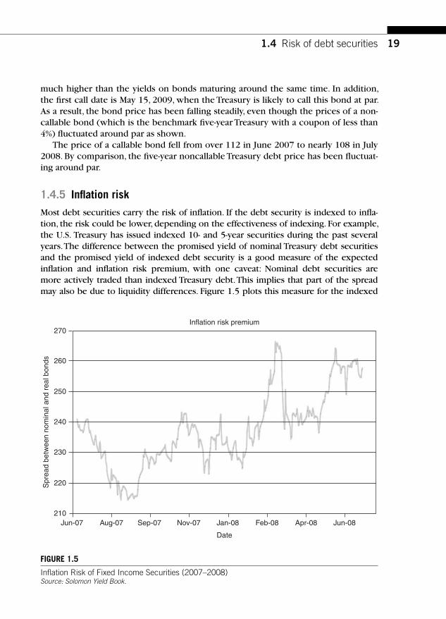
1.4.5 Infl ation risk
Most debt securities carry the risk of infl ation. If the debt security is indexed to infl a-tion, the risk could be lower, depending on the effectiveness of indexing. For example, the U.S. Treasury has issued indexed 10- and 5-year securities during the past several years. The difference between the promised yield of nominal Treasury debt securities and the promised yield of indexed debt security is a good measure of the expected infl ation and infl ation risk premium, with one caveat: Nominal debt securities are more actively traded than indexed Treasury debt. This implies that part of the spread may also be due to liquidity differences. Figure 1.5 plots this measure for the indexed
1.4 Risk of debt securities
270
260
250
240
230
220
210Jun-07 Aug-07 Sep-07 Nov-07 Jan-08 Feb-08 Apr-08 Jun-08
Date
Inflation risk premium
Spr
ead
betw
een
nom
inal
and
rea
l bon
ds
FIGURE 1.5
Infl ation Risk of Fixed Income Securities (2007 – 2008) Source: Solomon Yield Book.

20 CHAPTER 1 Overview of fi xed income markets
debt issued by the Treasury with a coupon of 2.75% and a maturity date of January 15, 2017. Note that the infl ation risk premium has fl uctuated from a low of about 210 basis points to a high of about 265 basis points. The indexed security compensates the investors for the realized infl ation rate, which includes both expected and unexpected infl ation rates. But the nominal debt security only compensates for the expected infl a-tion rate at the time it was issued. The difference between their promised yields is then a good measure of infl ation risk premium, subject to liquidity differences between these markets. (We examine the indexed bond markets in Chapter 13.)
1.4.6 Event risk
Some debt securities may be sensitive to events such as hostile reorganizations or leveraged buyouts (LBOs). Such events can lead to a signifi cant price loss.
In October 1988 RJR Nabisco was taken over through an LBO. The resulting com-pany took on heavy debt to fi nance the takeover. As a result, Moody’s rating of RJR Nabisco’s debt went from A1 to B3. The prices of RJR bonds dropped about 15%, and the yield spread went from about 100 basis points over Treasury to about 350 basis points over Treasury. In corporate debt securities this is referred to as event risk.
Investors often require protection against this type of risk by requiring a right from the sellers of bonds that allows the investors to sell (or put) the bonds back to the seller at par value. This provision has come to be known as the superpoison put provision.Warga and Welch (1993) examined the bondholder losses associated with “ LBO event ” and found that the cumulative losses to bondholders for 16 fi rms expe-riencing LBO events were nearly 7% within a 20-day window surrounding the event date, as shown in Figure 1.6 .
1.4.7 Tax risk
If debt securities were originally issued with certain tax exemption features and subsequently there developed an uncertainty regarding their tax status, it could lead to a price loss if the outstanding issues are not “grandfathered. ” This type of risk is especially relevant for municipal debt markets, which enjoy tax advantages that may change at the discretion of the U.S. Congress.
1.4.8 FX risk
Depending on the currencies in which the investor is domiciled, debt securities may pose FX risk as well; for example, for a Japanese pension fund that wants to fund lia-bilities in Yen, investments in U.S. Treasury securities will pose FX risk. Central banks of Japan and China hold signifi cant amounts of U.S. government debt as investments, and consequently they are subject to the risk that the dollar could depreciate.
The preceding discussions clearly suggest that Treasury debt securities are per-haps the least risky securities in fi xed income securities markets, holding all relevant factors the same. They do not have any credit risk, they are relatively liquid, and for

21
the most part they do not carry any contractual risks. For these reasons, investors are willing to pay a higher price to hold Treasury securities. Consequently their yields are lower.
Corporate securities trade at a yield spread over Treasuries to compensate inves-tors for credit risk, liquidity risk, timing risk, and so on. This spread is highly vari-able, as the GM example illustrates. Treasuries trade at a spread over municipal debt securities because municipal debt securities have certain exemptions from taxes. As a result, investors are prepared to hold municipal securities at a lower yield. The spread between Treasury and municipal debt securities is also variable.
All securities in fi xed-income markets are priced relative to the appropriate Treasury benchmark. Spreads depend on the risk factors we described earlier. We now turn to the historical performance of fi xed income markets as measured by broad fi xed income indexes.
1.5 RETURN-RISK HISTORY The Lehman aggregate index is a widely accepted benchmark used in the industry for judging the performance of debt securities markets in the aggregate. The index
1.5 Return-risk history
0.02
0.01 Risk/maturity adjusteddebt return
0
�13�12�11�10 �9 �8 �7 �6 �5 �4 �3 �2 �1 0 1 2 3 4 5 6 7 8
�0.01
�0.02
�0.03
�0.04
�0.05
�0.06
�0.07
�0.08
Event time in months
Cum
ulat
ive
retu
rn (
1 �
100
%)
FIGURE 1.6
Event Risk in Fixed Income Securities Source: A. Warga and I. Welch, “ Bondholder Losses in Leveraged Buyouts, ” Review of Financial Studies, 1993, Vol. 6, pp. 959 – 982.

22 CHAPTER 1 Overview of fi xed income markets
is constructed and updated as per rules that are transparent. The composition of the Lehman aggregate index as of December 2007 is shown in Figure 1.7 .
The Lehman aggregate index attempts to refl ect the composition of the overall debt markets. Comparing Figure 1.6 with Figure 1.5 we can see that the Lehman aggregate emphasizes Treasury debt much more than the overall market. The corporate and secu-ritized sector, which includes MBS, roughly corresponds to the overall market.
The historical returns for the Lehman aggregate index for the period 1992 through 2007 are shown next in Figure 1.8 .
It is clear that the aggregate index has provided exceptional returns during some years (1995, 2000, and 2001) and has performed dismally in other years (1994 and 1999). This suggests that, in the aggregate, debt securities have signifi cant volatility associated with their returns. The return-risk performances of various segments of the debt markets (such as Treasury, MBS, and the like) could differ from the Lehman aggregate index from year to year. We review their performances in later chapters.
To get a perspective on how fi xed income markets have performed over a long horizon relative to other asset classes in the economy, we take a look at Table 1.8 ,which covers the period 1988 –2007.
Overall, U.S. bonds have provided a return of 7.8% with a volatility of 4.2%. This is relatively low risk with correspondingly low returns compared to other asset classes such as equity. Note that the debt markets had the least number of periods with negative returns (69) compared to large-cap equity, which had 84 negative periods. Moreover, the lowest quarterly return for debt markets was �2.9%, whereas for the large-cap equity the lowest quarterly return was �17.3%. This is indicative of the fact that fi xed income markets, viewed in the context of broad indexes, are less risky than equity markets. It is also clear that the upside is somewhat limited: Large-cap equity had a highest quarterly return of 21.3%, whereas the highest quarterly return for bonds was just 8.0%.
Treasury47.7%
Government-related14.3%
Corporate16.8%
Securitized21.2%
FIGURE 1.7
Lehman Aggregate Index, December 2007 Source: Lehman Brothers.
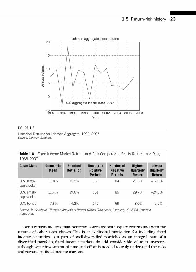
23
Bond returns are less than perfectly correlated with equity returns and with the returns of other asset classes. This is an additional motivation for including fi xed income securities as a part of well-diversifi ed portfolio. As an integral part of a diversifi ed portfolio, fi xed income markets do add considerable value to investors, although some investment of time and effort is needed to truly understand the risks and rewards in fi xed income markets.
1.5 Return-risk history
20
15
10
5
0
�51992 1994 1996 1998 20082000 20062002 2004
Year
Ann
ual r
etur
nsLehman aggregate index returns
U.S aggregate index: 1992–2007
FIGURE 1.8
Historical Returns on Lehman Aggregate, 1992 – 2007 Source: Lehman Brothers.
Table 1.8 Fixed Income Market Returns and Risk Compared to Equity Returns and Risk, 1988 – 2007
Asset Class Geometric Mean
Standard Deviation
Number of PositivePeriods
Number of NegativePeriods
Highest QuarterlyReturn
Lowest QuarterlyReturn
U.S. large-cap stocks
11.8% 15.2% 156 84 21.3% – 17.3%
U.S. small-cap stocks
11.4% 19.6% 151 89 29.7% – 24.5%
U.S. bonds 7.8% 4.2% 170 69 8.0% – 2.9%
Source: M. Gambera, “ Ibbotson Analysis of Recent Market Turbulence, ” January 22, 2008, Ibbotson Associates.

24 CHAPTER 1 Overview of fi xed income markets
SUGGESTED REFERENCES AND READINGS The Securities Industry and Financial Markets Association (SIFMA) is an excellent source for gaining an overview of securities markets in general and fi xed income markets in particular. Their Website is www.sifma.org . The International Capital Market Association (ICMA) is another excellent source for gaining insight into global capital markets. Their Website is www.icma-group.org . The Lehman aggregate index and its properties can be found at the Website of Lehman Brothers at www.lehman.com/fi /indices/ .
We relied on the following academic and policy research in this chapter. The original papers cited here examine the issues in much greater detail.
Barclay , M. J. , Hendershott , T. , & Kotz , K. ( 2006, October ) . Automation versus intermediation: Evidence from treasuries going off the run . Journal of Finance , LX1 ( 5) , 2395 – 2414 .
Gambera , M. ( 2008, 22 January ) . Ibbotson analysis of recent market turbulence. Ibbotson Associates .
Warga , A. , & Welch , I. ( 1993) . Bondholder losses in leveraged buyouts . Review of Financial Studies , 6 , 959 – 982 .

25
CHAPTER
Fixed Income Markets and Their DerivativesCopyright 2009 by Academic Press. Inc. All rights of reproduction in any form reserved.
CHAPTER SUMMARY This chapter outlines basic concepts of compounding and discounting. We show how to calculate the price of a debt security, given discount rates and contractual terms, including coupons and maturity. We provide several examples using Microsoft Excel and illustrate the pricing of Treasury bills, Treasury notes, and bonds. Concepts of accrued interest and yield to maturity are developed and illustrated. The convex relationship between price and yield of a debt security is shown in the context of real-life examples.
2.1 CONCEPTS OF COMPOUNDING AND DISCOUNTING The basics of time value of money and discounting are quite important in under-standing how fi xed income securities are valued. We review the time value concepts and illustrate the ideas with some examples in this section. Readers who are famil-iar with discounting concepts, annuities, and perpetuities can skip this section and move directly to Section 2. 2.
2.1.1 Future values
When they invest in debt securities, investors receive periodic coupons, which must be reinvested. The wealth accumulated by investors will then depend on the rates at which they are able to invest their coupon incomes. Likewise, the price at which they may be able to sell the security in the future will depend on the prevailing interest rates in the markets at the time of sale. We examine these issues now.
In addition, the rate at which money placed in coupon-bearing bond portfolio grows depends on the method used for computing the interest payments and rein-vestment assumptions. There are two methods of interest calculation: simple inter-est and compound interest. Compound-interest calculations vary with respect to the
Price-yield conventions 2
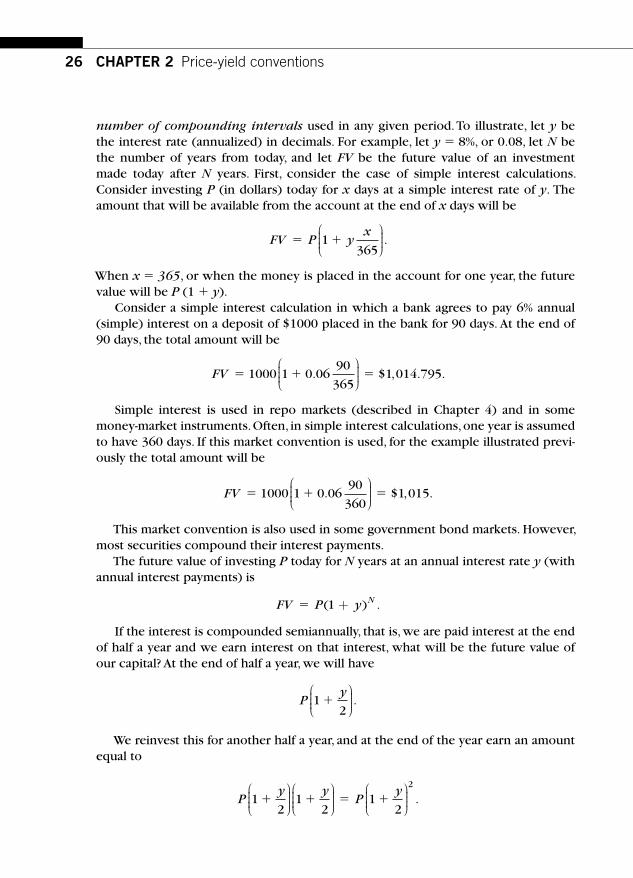
26 CHAPTER 2 Price-yield conventions
number of compounding intervals used in any given period. To illustrate, let y be the interest rate (annualized) in decimals. For example, let y � 8%, or 0.08, let N be the number of years from today, and let FV be the future value of an investment made today after N years. First, consider the case of simple interest calculations. Consider investing P (in dollars) today for x days at a simple interest rate of y. The amount that will be available from the account at the end of x days will be
FV P yx
� �1365
⎛⎝⎜⎜⎜
⎞⎠⎟⎟⎟.
When x � 365, or when the money is placed in the account for one year, the future value will be P (1 � y ).
Consider a simple interest calculation in which a bank agrees to pay 6% annual (simple) interest on a deposit of $1000 placed in the bank for 90 days. At the end of 90 days, the total amount will be
FV � � �1000 1 0 0690
3651 014 795. $ , . .
⎛⎝⎜⎜⎜
⎞⎠⎟⎟⎟
Simple interest is used in repo markets (described in Chapter 4) and in some money-market instruments. Often, in simple interest calculations, one year is assumed to have 360 days. If this market convention is used, for the example illustrated previ-ously the total amount will be
FV � � �1000 1 0 0690
3601 015. $ , .
⎛⎝⎜⎜⎜
⎞⎠⎟⎟⎟
This market convention is also used in some government bond markets. However, most securities compound their interest payments.
The future value of investing P today for N years at an annual interest rate y (with annual interest payments) is
FV P y N� ( ) .1 +
If the interest is compounded semiannually, that is, we are paid interest at the end of half a year and we earn interest on that interest, what will be the future value of our capital? At the end of half a year, we will have
Py
12
�⎛⎝⎜⎜⎜
⎞⎠⎟⎟⎟.
We reinvest this for another half a year, and at the end of the year earn an amount equal to
Py y
Py
12
12
12
2
� � � �⎛⎝⎜⎜⎜
⎞⎠⎟⎟⎟⎛⎝⎜⎜⎜
⎞⎠⎟⎟⎟
⎛⎝⎜⎜⎜
⎞⎠⎟⎟⎟ .

27
So, with semiannual compounding, the terminal value after one year is
FV Py
� �12
2⎛⎝⎜⎜⎜
⎞⎠⎟⎟⎟ .
Proceeding this way, the future value of setting aside P today for N years (with m compounding intervals per year) is
FV Py
m
N m
� �1⎛⎝⎜⎜⎜
⎞⎠⎟⎟⎟
×
.
As we increase the compounding interval, m, to infi nity, we get a future value with continuous compounding of
FV Pe yN� .
Generally, we can convert from one method of compounding to another. If we are given the annually compounded interest rate y* , we can convert it to the semian-nually compounded interest rate y using
12
12
� � �y
y⎛⎝⎜⎜⎜
⎞⎠⎟⎟⎟⎟ ( *).
Converting interest rates quoted under one convention (say, annual compounding) to another convention (say, semiannual compounding) is important because we need to compare the performances of different segments of the market under one conven-tion. For example, if the interest rate for an investment is quoted as 8% under annual compounding, on a semiannual compounding basis it will be 7.846%. We arrive at this fi gure by setting in the preceding equation y* %� 8 . Then, we solve for y as follows:
y � � � �2 1 08 1 0 07846 7 846. . . %.⎡⎣⎢
⎤⎦⎥
Table 2.1 records the future values of $100 at a 5% interest rate under annual, semiannual, quarterly, and continuous compounding. Note that the value differences resulting from the number of compounding intervals per year are rather small for maturities of 1 to 10 years. At the end of one year, the simple interest earned is $5, whereas with continuous compounding the interest earned is $5.13. Clearly, the more frequent the compounding, the more interest is earned on interest.
2.1.2 Annuities
A security that pays C (in dollars) per period for N periods is known as an annuity.We can determine the future value of an annuity that pays C for two years as follows: The fi rst year’s payment can be reinvested for one more year at a rate y to get, at the end of Year 2, an amount C y( ).1 �
This amount, added to the payment of C at the end of Year 2, gives a future value of
FV C C y� � �( ).1
2.1 Concepts of compounding and discounting

28 CHAPTER 2 Price-yield conventions
Multiplying the previous equation by ( )1 � y gives the following expression:
FV y C y C y( ) ( ) ( ) .1 1 1 2� � � � �
Subtracting the fi rst equation from the second and simplifying gives
FVC
yy� � �( ) .1 12⎡
⎣⎢⎤⎦⎥
In this way we can determine the future value of an annuity C for N years with an annual interest payment as follows:
FVC
yy N� � �( ) .1 1⎡
⎣⎢⎤⎦⎥
We illustrate the idea of an annuity with an example.
Example 2.1 Consider a loan in which a payment of C � 100 per annum has to be made for the next 10 years. Let the interest rate y be equal to 9%. What is the future value of this annuity?
The future value of this annuity at a reinvestment rate of 9% is
FV � � � �1000 09
1 0 09 1 1 519 2910
.( . ) , . .⎡⎣⎢
⎤⎦⎥
Table 2.1 Effect of Compounding Intervals on Future Values
Years to Maturity Annual ($) Semiannual ($) Quarterly ($) Continuous ($)
Compounding
1 105.00 105.06 105.09 105.13
2 110.25 110.38 110.45 110.52
3 115.76 115.97 116.08 116.18
4 121.55 121.84 121.99 122.14
5 127.63 128.01 128.20 128.40
10 162.89 163.86 164.36 164.87
20 265.33 268.51 270.15 271.83
30 432.19 439.98 444.02 448.17
50 1146.74 1181.37 1199.52 1218.25

29
Example 2.2 Consider a bond that pays a $10 coupon for three years (annually) and $100 par value at maturity. Assuming a 9% reinvestment rate, what is the future value of this bond after three years?
This bond is a portfolio of (a) an annuity paying $10 for the next three years and (b) a zero-coupon bond paying $100 after three years. Hence to compute the future value, we simply compute the future value of the annuity and then add to it the $100 to be received at maturity. The future value of a $10 annuity after three years is:
FV = ⎡⎣⎢
⎤⎦⎥
100 09
1 0 09 1 32 7813
.( . ) . .� � �
Adding the terminal payment of $100 to this quantity gives us the future value of $132.781.
Example 2.3 Let’s assume that an investor purchased this bond at a price of $100. What is the investor’s annualized return under the reinvestment assumption made?
Let r be the return (annualized). Then 100 1 132 7813( ) . .� �r Solving for r, we get the return as:
r � � � �132 781
1001 0 0991205 9 912053
.. . %.
For various reinvestment assumptions, we can compute the return experience for the investor.
2.1.3 Present values
For holders of securities, which promise cash fl ows at future dates, the concept of pres-ent value ( PV ) is important. What is the PV of $1 to be received N years from today? We can think of a zero-coupon bond that pays $1 after N years and nothing before. What should be the price of such a zero-coupon bond? Using the ideas we described earlier, the PVs can be formulated for various compounding periods as follows:
With annual compounding, the present value formula will be:
PVy N
��
1
1( ). (2.1)
Similarly, the PV of $1 received after N years with m interest compounding inter-vals per year is
PVy N m
��
1
1( ).
× (2.2)
2.1 Concepts of compounding and discounting
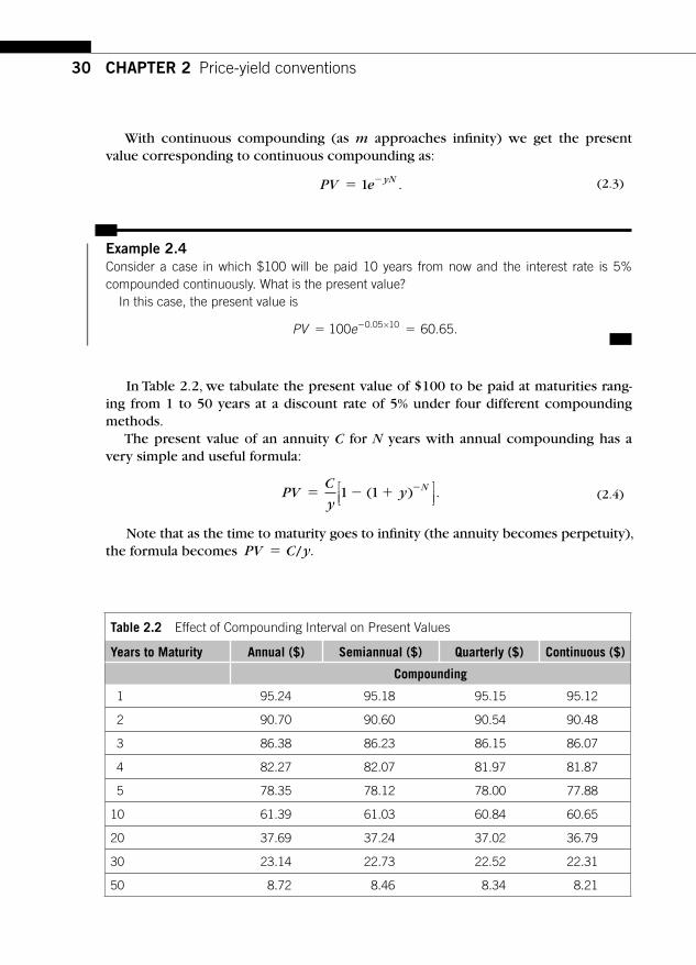
30 CHAPTER 2 Price-yield conventions
With continuous compounding (as m approaches infi nity) we get the present value corresponding to continuous compounding as:
PV e yN� �1 . (2.3)
Example 2.4 Consider a case in which $100 will be paid 10 years from now and the interest rate is 5% compounded continuously. What is the present value?
In this case, the present value is
PV e� ��100 60 650 05 10. . .×
In Table 2.2 , we tabulate the present value of $100 to be paid at maturities rang-ing from 1 to 50 years at a discount rate of 5% under four different compounding methods.
The present value of an annuity C for N years with annual compounding has a very simple and useful formula:
PVC
yy N� � � �1 1( ) .⎡
⎣⎢⎤⎦⎥ (2.4)
Note that as the time to maturity goes to infi nity (the annuity becomes perpetuity), the formula becomes PV C y� / .
Table 2.2 Effect of Compounding Interval on Present Values
Years to Maturity Annual ($) Semiannual ($) Quarterly ($) Continuous ($)
Compounding
1 95.24 95.18 95.15 95.12
2 90.70 90.60 90.54 90.48
3 86.38 86.23 86.15 86.07
4 82.27 82.07 81.97 81.87
5 78.35 78.12 78.00 77.88
10 61.39 61.03 60.84 60.65
20 37.69 37.24 37.02 36.79
30 23.14 22.73 22.52 22.31
50 8.72 8.46 8.34 8.21
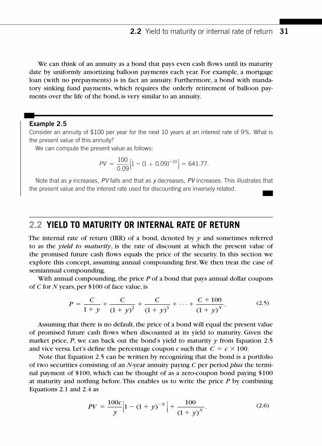
31
We can think of an annuity as a bond that pays even cash fl ows until its maturity date by uniformly amortizing balloon payments each year. For example, a mortgage loan (with no prepayments) is in fact an annuity. Furthermore, a bond with manda-tory sinking fund payments, which requires the orderly retirement of balloon pay-ments over the life of the bond, is very similar to an annuity.
Example 2.5 Consider an annuity of $100 per year for the next 10 years at an interest rate of 9%. What is the present value of this annuity?
We can compute the present value as follows:
PV � � ��1000 09
1 1 0 09 641 7710
.( . ) . .+⎡
⎣⎢⎤⎦⎥
Note that as y increases, PV falls and that as y decreases, PV increases. This illustrates that the present value and the interest rate used for discounting are inversely related.
2.2 YIELD TO MATURITY OR INTERNAL RATE OF RETURN The internal rate of return (IRR) of a bond, denoted by y and sometimes referred to as the yield to maturity, is the rate of discount at which the present value of the promised future cash fl ows equals the price of the security. In this section we explore this concept, assuming annual compounding fi rst. We then treat the case of semiannual compounding.
With annual compounding, the price P of a bond that pays annual dollar coupons of C for N years, per $100 of face value, is
PC
y
C
y
C
y
C
y N�
��
��
�� �
�
�1 1 1
100
12 3( ) ( ) ( ).⋅ ⋅ ⋅ (2.5)
Assuming that there is no default, the price of a bond will equal the present value of promised future cash fl ows when discounted at its yield to maturity. Given the market price, P, we can back out the bond’s yield to maturity y from Equation 2.5 and vice versa. Let’s defi ne the percentage coupon c such that C c� � 100.
Note that Equation 2.5 can be written by recognizing that the bond is a port folio of two securities consisting of an N-year annuity paying C per period plus the termi-nal payment of $100, which can be thought of as a zero-coupon bond paying $100 at maturity and nothing before. This enables us to write the price P by combining Equations 2.1 and 2.4 as
PVc
yy
yN
N� � � �
�
�1001 1
100
1( )
( ).⎡
⎣⎢⎤⎦⎥
(2.6)
2.2 Yield to maturity or internal rate of return
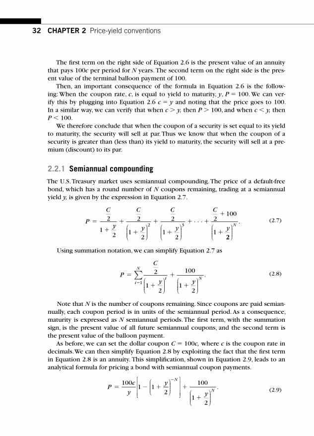
32 CHAPTER 2 Price-yield conventions
The fi rst term on the right side of Equation 2.6 is the present value of an annuity that pays 100 c per period for N years. The second term on the right side is the pres-ent value of the terminal balloon payment of 100.
Then, an important consequence of the formula in Equation 2.6 is the follow-ing: When the coupon rate, c, is equal to yield to maturity, y, P � 100. We can ver-ify this by plugging into Equation 2.6 c � y and noting that the price goes to 100. In a similar way, we can verify that when c � y, then P � 100, and when c � y, then P � 100.
We therefore conclude that when the coupon of a security is set equal to its yield to maturity, the security will sell at par. Thus we know that when the coupon of a security is greater than (less than) its yield to maturity, the security will sell at a pre-mium (discount) to its par.
2.2.1 Semiannual compounding
The U.S. Treasury market uses semiannual compounding. The price of a default-free bond, which has a round number of N coupons remaining, trading at a semiannual yield y, is given by the expression in Equation 2.7.
P
C
y
C
y
C
y
C
y�
�
�
�
�
�
� ��
�
2
12
2
12
2
12
2100
12 3⎛
⎝⎜⎜⎜
⎞⎠⎟⎟⎟
⎛⎝⎜⎜⎜
⎞⎠⎟⎟⎟
⋅ ⋅ ⋅
22
⎛⎝⎜⎜⎜
⎞⎠⎟⎟⎟
N. (2.7)
Using summation notation, we can simplify Equation 2.7 as
P
C
y yi
i
N
N�
�
�
��
2
12
100
12
1 ⎛⎝⎜⎜⎜
⎞⎠⎟⎟⎟
⎛⎝⎜⎜⎜
⎞⎠⎟⎟⎟
∑ . (2.8)
Note that N is the number of coupons remaining. Since coupons are paid semian-nually, each coupon period is in units of the semiannual period. As a consequence, maturity is expressed as N semiannual periods. The fi rst term, with the summation sign, is the present value of all future semiannual coupons, and the second term is the present value of the balloon payment.
As before, we can set the dollar coupon C � 100 c, where c is the coupon rate in decimals. We can then simplify Equation 2.8 by exploiting the fact that the fi rst term in Equation 2.8 is an annuity. This simplifi cation, shown in Equation 2.9, leads to an analytical formula for pricing a bond with semiannual coupon payments.
Pc
y
y
y
N
N� � � �
�
�100
1 12
100
12
⎛⎝⎜⎜⎜
⎞⎠⎟⎟⎟
⎡
⎣
⎢⎢⎢
⎤
⎦
⎥⎥⎥ ⎛
⎝⎜⎜⎜
⎞⎠⎟⎟⎟
. (2.9)

33
Using Equation 2.9 we can determine the price, P, of a bond, given its yield to maturity y. Alternatively, we can determine the yield, y, of a bond, given its price P.There is a simple case when N goes to infi nity. This special case is known as a perpe-tuity, which pays every six months a dollar coupon of C. From Equation 2.9 we solve for the price of perpetuity as follows:
Pc
y�
100. (2.10)
Often, in practice a concept known as current yield, denoted by ycurrent , is used. The current yield of a bond is its dollar coupon divided by its price, as shown here:
yC
P
c
Pcurrent � �100
. (2.11)
Current yield measures the dollar coupon income as a fraction of the market price of the bond. It is an approximation of yield to maturity. Only for perpetuity, current yield will be the same as its yield to maturity.
The formula shown in Equation 2.9 assumes that the bond has no fractional cou-pon periods; in other words, we always value the bond on a coupon date. In reality, the settlement date may fall between two coupon dates, resulting in a fractional cou-pon period. We consider this idea later in the chapter.
2.3 PRICES IN PRACTICE It is customary in fi xed-income markets to quote values in terms of yields and/or prices. As we noted in the previous section, given a yield to maturity, we can com-pute the price, and vice versa. Although the process of quoting prices in decimals has begun in the stock market, the prices in fi xed income securities markets are not always quoted in decimals. Treasury prices are typically quoted in 32nds and some-times in units of 32nds, as made clear in the quotes that follow.
For example, recently the benchmark Treasury securities were quoted as shown in Table 2.3 .
2.3 Prices in practice
Table 2.3 Treasury Quotes as of June 26, 2008
Maturity in Years Quoted Price (in Units of 32nds)
Computed Price (Decimals)
2 100-13� 100.421875
5 100-15� 100.484375
10 98-22 98.687500
30 96-10� 96.312500
Source: Bloomberg.

34 CHAPTER 2 Price-yield conventions
For example, the price of a two-year Treasury note is 10013
32
1
64� � �
100.421875. All the computed prices are shown in the last column of the table. Note
that the symbol � denotes 1
64th. Sometimes the symbol � � is used to denote 1
128th.
We need to convert prices to decimals to perform fi nancial calculations. The prices that are quoted in 32nds (or any other fraction) can be converted to decimals using the Excel function shown next. In a similar manner, we can report a computed price (which will typically be in decimals) into 32nds as shown in Figure 2.1 .
2.4 PRICES AND YIELDS OF T-BILLS We start with the concept of invoice price (or dirty price) of a security. Invoice price is the price that the buyer of a security has to pay. We fi rst begin with Treasury bills, which are discount instruments; they do not pay any coupons and pay a fi xed sum of money (say, $100) at a stated maturity date. Conceptually T-bills are zero-coupon bonds.
25
26
27
28
29
30
31
32
33
34
35
36
37
38
39
40
41
K L M N O P Q
Converting quotes into decimals
Maturity Quoted Price
Price in decimals
(In 32nds)
10 98.22 98.6875 � DOLLARDE (L30,32)
Converting a computed price in decimals to a quote in 32nds
Maturity Quoted Price
Price in decimals
(In 32nds)
10 98.22 98.6875
= DOLLARFR (M39,32)
FIGURE 2.1
Excel Functions for Converting Quotes to Decimals, and Vice Versa

35
Treasury bills are quoted on a discount yield basis. The procedure for obtaining the invoice price from discount quotes is illustrated in the next example, in which quotations for settlement on June 26, 2008, for three- and six-month U.S. Treasury bills are shown in Table 2.4 .
Example 2.6 The invoice price, P , using the discount yield is then calculated as follows:
Pn d
� ��
100 1360
⎡
⎣⎢⎢
⎤
⎦⎥⎥. (2.12)
where the T-bill has n days remaining from the settlement date to maturity and has a discount yield d per $100 face amount. For the three-month T-bill, the price is computed as follows:
P � ��
�100 190 0 0168
36099 58
.. .
⎡
⎣⎢⎢
⎤
⎦⎥⎥
The number of days to maturity ( n) is the difference between the maturity date and the settlement date. P is a percentage of the par amount of the Treasury bill. T-bills are typically traded in $1 million par, so that the invoice price per million will be $995,800.
2.4.1 Yield of a T-Bill with n < 182 Days
We can rewrite the price formula of Equation 2.12 to get an expression for the dis-count rate of T-bills as follows:
dP
n�
��
100
100
360. (2.13)
Note that the discount yield has two shortcomings. It uses 360 days per year and it divides the dollar gain (or discount), 100 � P, by 100 rather than by P. The bond equivalent yield, or BEY , corrects these two shortcomings. For a T-bill with a matu-rity of fewer than 182 days, the BEY is calculated as
BEYP
P n�
��
100 365. (2.14)
2.4 Prices and yields of T-bills
Table 2.4 Market Quotes for T-Bills as of June 26, 2008 (Settlement on June 27, 2008)
Maturity Date Discount Time to Maturity (Days)
Price ($) BEY
3-month 9/25/2008 1.68% 90 99.58 1.71%
6-month 12/26/2008 2.10% 182 98.94 2.15%
Source: Bloomberg.

36 CHAPTER 2 Price-yield conventions
The BEY of T-bills is a better measure of the actual return that investors will get by buying the T-bill and holding it until its maturity date. Using the formulas for discount rate and BEY, we can identify a simple relation between the discount yield d that traders quote and the BEY as follows:
BEYd
nd�
�
365
360. (2.15)
Thus, using the discount quote of 1.68% for the T-bill with 90 days to maturity, we get a BEY of 1.71% as follows:
BEY ��
� ��
365 0 0168
360 90 0 01681 71
.
( . ). %.
Similarly, using the discount quote of 2.10%, we get a BEY of 2.15% for the T-bill with 182 days to maturity.
Note that the BEY is always greater than d. This is hardly surprising given that we obtain BEY by dividing the dollar discount by P (which is less than 100) and mul-tiplying the result by 365 (which is more than 360). The difference between BEY and d increases with time to maturity. This can be seen in Figure 2.2 , where we have plotted the difference between the BEY and discount yield (in basis points) of all T-bills as of July 25, 2008.
2.4.2 Yield of a T-Bill with n > 182 Days
When a T-bill has more than six months to maturity, the calculation must refl ect the fact that a T-bill does not pay interest, whereas a T-note or T-bond will pay a semiannual
BEY minus discount yield
2.000
3.000
4.000
5.000
6.000
7.000
8.000
7/13/08 9/1/08 10/21/08 12/10/08 1/29/09 3/20/09 5/9/09 6/28/09 8/17/09
Maturity
BE
Y m
inus
dis
coun
tyi
eld
(bps
)
FIGURE 2.2
Differences Between BEY and Discount Yield, July 13, 2008–August 17, 2009

37
interest. The industry convention is to assume that an interest y is paid after six months and that it is possible to reinvest this interest, that is,
Py y
ny
P12 365
365
21
2100� � � � �
⎛⎝⎜⎜⎜
⎞⎠⎟⎟⎟
⎛⎝⎜⎜⎜
⎞⎠⎟⎟⎟⎛⎝⎜⎜⎜
⎞⎠⎟⎟⎟ .
The fi rst term in the preceding equation computes the dollar value of initial investment in the T-bill reinvested on a semiannual basis for one coupon period. The second term measures the interest earned on this amount for the remaining time to the maturity date of the T-bill.
Solving for y gives the BEY for T-bills with a maturity of more than 182 days as
BEY
n n n
P�
� � � � �2
3652
365
2
3651 1
1002⎛
⎝⎜⎜⎜
⎞⎠⎟⎟⎟
⎛⎝⎜⎜⎜
⎞⎠⎟⎟⎟⎛⎝⎜⎜⎜
⎞⎠⎟⎟⎟⎟
2
3651
n�
. (2.16)
It turns out that Excel has convenient functions to calculate BEY and T-bill prices of any maturity. We illustrate the applications of T-bill-related Excel functions in Figure 2.3 .
Thus, by applying the � TBILLPRICE function, we can determine the price of a T-bill, knowing (a) the settlement date, (b) the maturity date, and (c) the quoted dis-count yield. Likewise, by applying the � TBILLEQ function, we can determine the BEY of the T-bill.
2.5 PRICES AND YIELDS OF T-NOTES AND T-BONDS For T-notes and T-bonds, the quoted price (also referred to as the clean or fl at price) is typically not the invoice price. To arrive at the invoice price (also referred to as the dirty price), we add the accrued interest to the fl at price. The accrued interest
2.5 Prices and yields of T-notes and T-bonds
54
55
56
57
58
59
60
61
62
63
K L M N O P Q R
T-Bill Quotes as of June 26, 2008
Settlement Date 6/27/2008
Maturity Discount Time to Price BEY
Maturity
3-Month 9/25/2008 1.68% 90 99.58 1.71% � TBILLEQ($N$57,L60,M60)
6-Month 12/26/2008 2.10% 182 98.94 2.15%
� TBILLPRICE ($N$57,L61,M61)
FIGURE 2.3
Excel T-Bill Functions

38 CHAPTER 2 Price-yield conventions
is the coupon income that accrues from the last coupon date to the settlement date of the transaction. This accrues to the seller of the security and must be paid by the buyer to get the full dollar coupon on the next coupon date. The following example illustrates this idea.
Example 2.7 The quotations for June 26, 2008, of a U.S. Treasury note with a 3.875% coupon and a matu-rity date of May 15, 2018, appear in Figure 2.4 . Recall that the price quotations are in 32nds.
Maturitydate
Coupon Quotedclean pricein decimals
5/15/2018 3.875% 98-22 98.6875
Quotedclean pricein 32nds
FIGURE 2.4
Market Quotes for Treasury NoteSource: Bloomberg.
First we compute the accrued interest. To do this, we determine the last coupon date (LCD), or the dated date (when the fi rst coupon starts to accrue), which in this case is May 15, 2008. This is also referred to as the previous coupon date (PCD). The next coupon date (NCD) is November 15, 2008. So, the number of days between the NCD and the LCD is 184 days. The number of days between the last coupon date and the settlement date, June 27, 2008, is 43 days. The accrued interest AI is
AI � �43
184
3 875
20 452785×
.. .
The quoted (clean) price is 98.22 (in 32nds) and is equal to 98.6875 (in deci-mals). Then the invoice (dirty) price is 98.6875 � 0.452785 � 99.140285.
The dirty price is a percentage of the principal amount, which is usually $1 million. The dirty price per million in this example is, therefore, $991,402.85 per million par.
All the calculations that we have performed can be executed via Excel functions as illustrated in Figure 2.5 .
There is an Excel function that can directly compute the accrued interest but requires as an input the issue date. The U.S. Treasury Website provides the issue date of all outstanding Treasury issues. We illustrate the use of that Excel function in Figure 2.6 .
The concept of yield to maturity that we have used so far can be extended to Treasury coupon issues with more than one coupon date remaining before the maturity date. Consider a Treasury bond that matures at date T. Let’s assume that the settlement date is t � T and that there are N coupon dates remaining. Let z be

39
the number of days between the settlement date and the next coupon date and x be the number of days between the last coupon date and the next coupon date. Then, given the invoice price Pt , the relation between Pt and y is
P
yt
Nz
x
�
�� �
100
12
1⎛⎝⎜⎜⎜
⎞⎠⎟⎟⎟
⎛
⎝
⎜⎜⎜⎜⎜⎜⎜⎜⎜⎜⎜⎜⎜⎜
⎞
⎠
⎟⎟⎟⎟⎟⎟⎟⎟⎟⎟⎟⎟⎟⎟⎟⎟⎛⎝⎜⎜⎜
⎞⎠⎟⎟⎟
∑�
���
� �C
yj
z
xj
j N2
12
0
1
. (2.17)
We can use this formula to fi nd the price Pt given the yield to maturity y, or we can solve for y given the price Pt .
Equation 2.17 is the appropriate price-yield relation, even when there are frac-tional coupon periods. In the next example we illustrate its application in deter-mining the yield to maturity of a Treasury bond for which the settlement date falls between two coupon dates. This formula can be implemented in Excel easily as shown next for calculating the yield of the 10-year T-note, given its market price.
2.5 Prices and yields of T-notes and T-bonds
6789
10111213141516171819202122232425262728
C D E F GSettlement Date (SD): 6/27/08
Maturity Coupon Quoted Clean
Date (MD) Price PriceClean in (Decimals)
32nds5/15/18 3.875% 98-22 98.687500
Issue Date 5/15/08
First Coupon Date 11/15/08
Next Coupon Date (NCD): 15-Nov-08 �COUPNCD($E$6,$C$12,2,1)
Last Coupon Date (LCD): 15-May-08 �COUPPCD($E$6,$C$12,2,1)
Number of Days Accrued: 43 �COUPDAYBS(E6,C12,2,1)
Basis (Number of Days between NCD and LCD): 184 � COUPDAYS(E6,C12,2,1)
Accrued Interest 0.452785 � (D12*100/2)*(E21/E24)
Dirty Price = 99.140285 � E26�F12
FIGURE 2.5
Excel Functions for Bonds

40 CHAPTER 2 Price-yield conventions
Example 2.8 To apply the price-yield formula, we need to set up the Excel spreadsheet as shown in Figure 2.7 . The following steps are followed in constructing the spreadsheet:
1. The fractional coupon period remaining is calculated as z/x, which is the ratio of remaining days to next coupon (from the settlement date) to the basis. In our example z � 141 and x � 182. Therefore, z/x is 0.766 (rounded to three decimals).
The remaining number of coupons, N, is 20. 2. The accrued interest as calculated before is 0.452785 (see Figures 2.5 and 2.6 ). 3. The dirty price of the T-note is clean price (98.6875) plus accrued interest (0.4527815)
and is equal to 99.140285. 4. We can identify for each coupon payment date the time to the payment date in semian-
nual periods as shown in the spreadsheet in column D. 5. We can then apply the price-yield formula (Equation 2.17) to get the present value of
all cash fl ows and sum them as done in column E. In cell E42 we have the sum of the present value of all cash fl ows as given by the price-yield formula.
6. We then use the Excel Solver to guess the correct yield to maturity (in cell E13) at which the sum of discounted cash fl ows (in cell E42) will be exactly equal to 99.140285, which is the dirty price of the T-note.
32
33
34
35
36
37
38
39
40
41
42
43
44
45
46
47
48
49
C D E F G
Settlement Date (SD): 6/27/08
Maturity Coupon Quoted Clean
Date (MD) Price Price
(Clean in 32nds)
5/15/18 3.875% 98-22 98.687500
Issue Date 5/15/08
First Coupon Date 11/15/08
Settlement Date (SD): 6/27/08
Coupon 3.875%
Accrued Interest 0.452785 � ACCRINT(E44,E45,E46,E47,100,2,1)
(Decimals)
FIGURE 2.6
Excel Function for Accrued Interest

41
Note that we could also use the Excel function � YIELD to compute the yield given price. This is also illustrated in cell F10. Note that this function takes as one of its inputs the clean price expressed in decimals.
2.5 Prices and yields of T-notes and T-bonds
123456789
101112131415161718192021222324252627282930313233343536373839404142
A B C D E F G H I
Yield given price
Settlement Date (SD): 6/27/08Fixed Income Markets and Their Derivatives
Maturity Coupon Quoted Clean YieldDate (MD) Price Price to Maturity
(in 32nds) (Decimals)
5/15/18 3.875% 98-22 98.6875 4.0369% <-- � YIELD(D4,B10,C10,E10,100,2,1)
Yield 4.0369%<-- By EXCEL Solver
Coupon Cash Time to PresentDates Payments Payment Value
in Semi-Annual of CashPeriods Payments
1 11/15/08 1.9375 0.766 1.908 <-- � C20/(1�$E$13/2)^D202 5/15/09 1.9375 1.766 1.8703 11/15/09 1.9375 2.766 1.8334 5/15/10 1.9375 3.766 1.7975 11/15/10 1.9375 4.766 1.7616 5/15/11 1.9375 5.766 1.7277 11/15/11 1.9375 6.766 1.6928 5/15/12 1.9375 7.766 1.6599 11/15/12 1.9375 8.766 1.626
10 5/15/13 1.9375 9.766 1.59411 11/15/13 1.9375 10.766 1.562 <-- � C30/(1+$E$13/2)^D3012 5/15/14 1.9375 11.766 1.53213 11/15/14 1.9375 12.766 1.50114 5/15/15 1.9375 13.766 1.47215 11/15/15 1.9375 14.766 1.44216 5/15/16 1.9375 15.766 1.41417 11/15/16 1.9375 16.766 1.38618 5/15/17 1.9375 17.766 1.35819 11/15/17 1.9375 18.766 1.33220 5/15/18 1.9375 19.766 1.305
5/15/18 100 19.766 67.368 <-- � C40/(1+$E$13/2)^D40
Sum of Present Value of Cash Flows: 99.140285 <-- � SUM(E20:E40)
FIGURE 2.7
Computing Yield to Maturity Using Excel Solver
In a similar manner, we can compute the price of a Treasury debt security given its yield. We illustrate this calculation next. Let’s consider the same security but assume that we only know the yield to maturity and that we want to calculate the price. We know that the worksheet that we developed earlier will give the correct dirty price of the Treasury note. We only need to subtract the accrued interest to get the correct clean price.
Excel has a � PRICE function that automatically returns the clean price (in deci-mals), given yield to maturity. Figure 2.8 illustrates this function.

42 CHAPTER 2 Price-yield conventions
2.6 PRICE-YIELD RELATION IS CONVEX As we increase the yield to maturity, the price will decline in general. This is due to the fact that the dollar coupon on debt securities is fi xed, and therefore, to com-pensate for the increases in yields in the market, the price must fall. We examine the behavior of price as yield to maturity is increased from 0% to 15% to gauge the price-yield relationship. The results are presented in Figure 2.9 .
Note that the prices fall as yields increase, but the rate of drop in price actu-ally goes down at higher yields. The convex relationship between price and yield to maturity of a debt security is an important feature in understanding how the value of debt security changes when rates in the market move. A drop of 400 basis points from 4% to 0% produces a price increase from 98.98 to 138.30, which is an increase of 39.72%. On the other hand, an increase of 400 basis points from 4% to 8% pro-duces a price loss from 98.98 to 72.18, which is a decrease of 27.08%.
In deriving this relationship, we have assumed that the T-note is a “bullet” security with no call feature. We will see later that the price-yield relationship is more com-plicated when there are call features.
This is due to the fact that an investor holding a callable bond faces the risk that the bond may be called away by the issuer when interest rates go down or when the issuer’s credit rating improves, or both. These circumstances will warrant the issuer to refi nance the old (callable debt) with cheaper new debt. As a result, a callable bond will not show the price increase in a regime of falling interest rates, as shown in Figure 2.10 . Instead, a callable bond price will approach the call price as interest rates fall. This feature is important for callable corporate debt, mortgages that have prepayments, and mortgage-backed securities.
2.7 CONVENTIONS IN OTHER MARKETS Conventions differ from one market to another. It is not practical to try to summarize the conventions of different markets, but it is helpful to note the following: In the
2
3
4
5
6
7
8
9
10
B C D E F G H
Price Given Yield
Settlement Date (SD): 6/27/08
Maturity Coupon Quoted Yield Clean
Date (MD) Price to Maturity Price
(in 32nds) (Decimals)
5/15/18 3.875% 98.22 4.0369% 98.6875 � PRICE(D4,B10,C10,E10,100,2,1)
FIGURE 2.8
Price, Given Yield

432.7 Conventions in other markets
6789
10111213141516171819202122232425262728293031323334353637383940414243
A B C D E F
Price Given Yield
Settlement 6/27/08Date (SD):
CleanPrice
(Decimals) Coupon 3.875%Maturity Date 5/15/18
� PRICE($F$9,$F$12,$F$11,B16,100,2,1)
Yieldto Maturity
0.0%0.5%1.0%1.5%2.0%2.5%3.0%3.5%4.0%4.5%5.0%5.5%6.0%6.5%7.0%7.5%8.0%8.5%9.0%9.5%10.0%10.5%11.0%11.5%12.0%12.5%13.0%13.5%14.0%14.5%15.0%
138.30132.50126.99121.74116.74111.97107.43103.1198.9895.0591.3187.7384.3281.0777.9775.0172.1869.4866.9064.4462.0959.8457.7055.6453.6851.8150.0148.3046.6545.0843.58
FIGURE 2.9
Convexity of Price-Yield Relation
United States, corporate bonds are quoted on the basis of 30/360-day counting con-ventions. When corporate bonds are callable, the yield computations are computed assuming that the bond will be called on each call date and the highest of the result-ing yields is reported as yield to worst. Agency debt securities are also reported on the basis of the 30/360 convention. Remembering that Treasury securities are reported on the basis of “ actual-actual, ” it becomes important to have a common convention for
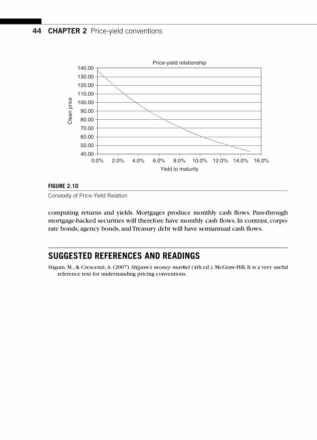
44 CHAPTER 2 Price-yield conventions
computing returns and yields. Mortgages produce monthly cash fl ows. Pass-through mortgage-backed securities will therefore have monthly cash fl ows. In contrast, corpo-rate bonds, agency bonds, and Treasury debt will have semiannual cash fl ows.
SUGGESTED REFERENCES AND READINGS Stigum, M., & Crescenzi, A. (2007). Stigum’s money market (4th ed.). McGraw-Hill. It is a very useful
reference text for understanding pricing conventions .
Price-yield relationship
40.00
50.00
60.00
70.00
80.00
90.00
100.00
110.00
120.00
130.00
140.00
0.0% 2.0% 4.0% 6.0% 8.0% 10.0% 12.0% 14.0% 16.0%
Yield to maturity
Cle
an p
rice
FIGURE 2.10
Convexity of Price-Yield Relation

45
CHAPTER
Fixed Income Markets and Their DerivativesCopyright 2009 by Academic Press. Inc. All rights of reproduction in any form reserved.
CHAPTER SUMMARY The key roles played by central banks are described in this chapter. The Fed’s openmarket operations and its role as the lender of last resort are discussed. The mecha-nisms the Fed uses for promoting fi nancial stability, orderly growth, and price sta-bility are explained. The historical behavior of target fed funds rate and effective Fed funds rates are presented and analyzed. The relationship between effective Fed funds rates and LIBOR is discussed. The chapter ends with a brief analysis of the actions taken by the Fed to combat the credit crisis of 2007 – 2008.
3.1 CENTRAL BANKS The central bank of a country is solely responsible for formulating and implement-ing the nation’s monetary policies. In addition, it is also responsible for several major functions in the stewardship of the banking sector and capital markets. In the United States, the central bank is referred to as the Federal Reserve, or, simply, the Fed. In other countries and economic zones, the term central bank or reserve bank is used. For example, the European Central Bank (ECB) is the central bank that governs mon-etary policies in the European zone. In Australia and India, for example, the central bank is referred to as the Reserve Bank.
The Fed consists of a Board of Governors and the Federal Reserve District Banks. Currently there are 12 district banks, each with its own branches. The Federal Reserve Board has seven members, one of whom serves as the Chairman. The President of the United States appoints all the members. The Federal Reserve has a committee known as the Federal Open Market Committee (FOMC), which authorizes the tools by which the Fed conducts monetary policies. Additional details pertaining to the organization of the Federal Reserve System may be found at the Website of the Board of Governors.
Federal Reserve (central bank) and fi xed income markets 3

46 CHAPTER 3 Federal Reserve (central bank) and fi xed income markets
The major functions of a central bank are to:
■ Formulate and execute monetary policies to promote orderly growth and price stability. These policies are keenly watched by the market participants, who form expectations about future actions of the central banks and incor-porate those expectations into market prices. To the extent that announced policies may differ from market participants ’ expectations, there can be a price reaction on the date when the FOMC makes its announcement. The Fed attempts to guide the “market ” about its perception of the state of the econ-omy through various communications.
■ Ensure the stability and integrity of banking and fi nancial markets. ■ Operate and regulate the funds fl ow and payments in the economy.
The Fed’s monetary policies control the supply of money and near-money instru-ments in the economy and the level and the course of interest rates of various maturities. In addition, as the central bank of the country, the Fed is the “lender of last resort. ” It also acts as an agent of the Treasury in conducting auctions and in handling payments and collections via electronic transfer systems. In addition, the central banks may perform several other supervisory and regulatory activities. For example, the Fed engages in the supervision of banks and provides banking and fi nancial services to other central banks and international fi nancial institutions.
3.2 MONETARY POLICIES The Federal Reserve is responsible for the country’s monetary policy. The Federal Reserve Act spells out the goals of the monetary policy as follows —to promote effectively the goals of:
■ Maximum employment (economic growth) ■ Stable prices (low to moderate infl ation) ■ Moderate long-term interest rates
There is a potential tension between maximizing employment and stabilizing prices; for example, a more moderate growth may be helpful in stabilizing prices. The Fed relies on three policy tools to execute its monetary policy. They are (a) open market operations, (b) discount window, and (c) reserve requirements. We describe each of these policy options next.
3.2.1 Open market operations
As noted earlier, the FOMC authorizes the tools by which it conducts monetary poli-cies. One of the mechanisms the Fed uses is to announce a rate known as the target Fed funds rate. By announcing this rate and using its policies (described later) to keep the short-term interest rates close to the announced target rate, the Fed attempts to infl uence interest rates and hence the cost of credit in the economy. The Fed’s policies
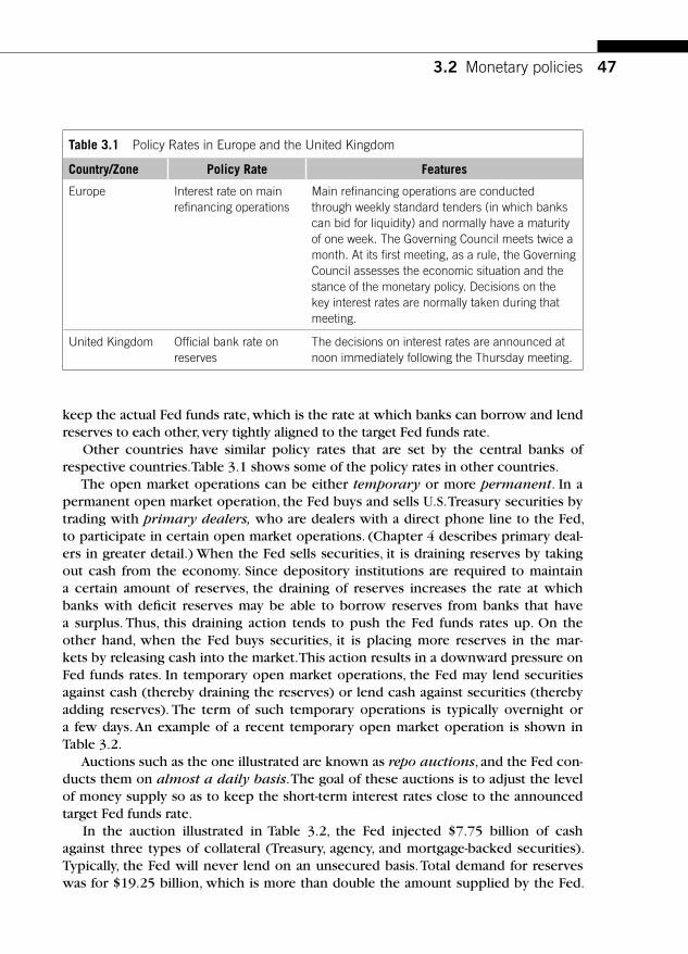
47
keep the actual Fed funds rate, which is the rate at which banks can borrow and lend reserves to each other, very tightly aligned to the target Fed funds rate.
Other countries have similar policy rates that are set by the central banks of respective countries. Table 3.1 shows some of the policy rates in other countries.
The open market operations can be either temporary or more permanent. In a permanent open market operation, the Fed buys and sells U.S. Treasury securities by trading with primary dealers, who are dealers with a direct phone line to the Fed, to participate in certain open market operations. (Chapter 4 describes primary deal-ers in greater detail.) When the Fed sells securities, it is draining reserves by taking out cash from the economy. Since depository institutions are required to maintain a certain amount of reserves, the draining of reserves increases the rate at which banks with defi cit reserves may be able to borrow reserves from banks that have a surplus. Thus, this draining action tends to push the Fed funds rates up. On the other hand, when the Fed buys securities, it is placing more reserves in the mar-kets by releasing cash into the market. This action results in a downward pressure on Fed funds rates. In temporary open market operations, the Fed may lend securities against cash (thereby draining the reserves) or lend cash against securities (thereby adding reserves). The term of such temporary operations is typically overnight or a few days. An example of a recent temporary open market operation is shown in Table 3.2 .
Auctions such as the one illustrated are known as repo auctions, and the Fed con-ducts them on almost a daily basis. The goal of these auctions is to adjust the level of money supply so as to keep the short-term interest rates close to the announced target Fed funds rate.
In the auction illustrated in Table 3.2 , the Fed injected $7.75 billion of cash against three types of collateral (Treasury, agency, and mortgage-backed securities). Typically, the Fed will never lend on an unsecured basis. Total demand for reserves was for $19.25 billion, which is more than double the amount supplied by the Fed.
3.2 Monetary policies
Table 3.1 Policy Rates in Europe and the United Kingdom
Country/Zone Policy Rate Features
Europe Interest rate on main refi nancing operations
Main refi nancing operations are conducted through weekly standard tenders (in which banks can bid for liquidity) and normally have a maturity of one week. The Governing Council meets twice a month. At its fi rst meeting, as a rule, the Governing Council assesses the economic situation and the stance of the monetary policy. Decisions on the key interest rates are normally taken during that meeting.
United Kingdom Offi cial bank rate on reserves
The decisions on interest rates are announced at noon immediately following the Thursday meeting.

48 CHAPTER 3 Federal Reserve (central bank) and fi xed income markets
A total of $0.20 billion was offered against Treasury collateral, $2.80 billion was offered against agency collateral, and $4.75 billion was provided against mortgage-backed securities. Dealers who posted Treasury collateral got cash at 2.19%, dealers who posted agency securities got cash at 2.22%, and those who posted mortgage-backed securities got cash at 2.30%.
This tool (repo auctions) allows the Fed to monitor and act on a daily basis as needed to respond to the demand for reserves in the economy and keep the short-term rates at the desired levels (namely, close to the target rate of interest).
3.2.2 The discount window
The discount window of the Federal Reserve is where the central bank lends funds to depository institutions as a “lender of last resort. ” The Federal Reserve Bank of New York reported that the Reserve banks lent $45.5 billion to depository institu-tions on September 12, 2001, the record for a single day. The Fed took this extraor-dinary action to calm the fi nancial markets on the day following the attack on the World Trade Center. Lending through the discount window typically takes the form of short-term adjustment credit, seasonal credit, and, in some instances, longer-term credit. The Discount window plays a complementary role to the open market opera-tions of the Fed. It is best thought of as a safety valve in relieving pressures in reserve markets. The discount window, by providing credit, has the potential to relieve illi-quidity in the banking system.
Prior to 2003, the credit from the discount window was offered at a discount to the target Fed funds rate and was rarely availed by fi nancial institutions for fear of the loss of reputation. The very act of a bank borrowing from the discount window may mark that bank as a “problem bank, ” leading other banks to curtail their
Table 3.2 Open Market “Repo Auctions ” by the Fed
Deal Date: June 27, 2008 Delivery Date: June 27, 2008
Maturity Date: July 1, 2008
Type of Operation
Repo
Results
Collateral Type
Amount ($ Billions) Rate (%)
Submitted Accepted Stop-Out Weighted Average
High Low
Treasury 2.050 0.200 2.190 2.190 2.190 1.750
Agency 7.700 2.800 2.220 2.261 2.33 2.1
Mortgage- backed
9.5 4.75 2.3 2.306 2.35 1.95
Total 19.25 7.75 — — — —
Source: Federal Reserve Bank of New York.

49
exposure to that bank. Hence a rational bank might never want to be seen at the dis-count window to borrow cash. This is sometimes referred to as the stigma effect.
Effective January 2003, the Fed has introduced (a) primary and (b) secondary credit programs. Primary credit is available to generally sound depository institutions on a very short-term basis, typically overnight, at a rate above the Federal Open Market Committee’s target rate for federal funds. When it was originally set up, the primary credit was available at a spread of 100 basis points over the target rate. Depository institutions are not required to seek alternative sources of funds before requesting occasional short-term advances of primary credit. The Federal Reserve expects that, given the above-market pricing of primary credit, institutions will use the discount window as a backup rather than a regular source of funding.
Secondary credit is available to depository institutions not eligible for primary credit. It is extended on a very short-term basis, typically overnight, at a rate that is above the primary credit rate. Secondary credit is available to meet backup liquidity needs when its use is consistent with a timely return to a reliance on market sources of funding or the orderly resolution of a troubled institution. Secondary credit may not be used to fund an expansion of the borrower’s assets. Table 3.3 describes the costs of borrowing at the discount window during the period January 2003 through April 2008.
Note that the Fed kept the premium of the rate charged in the primary credit facility at 100 basis points over the target Fed funds rates from January 2003 until July 2007. The onset of the credit crunch resulted in the Fed fi rst cutting this pre-mium to 50 basis points over the target rate in August 2007. The premium was fur-ther slashed to 25 basis points in March 2008. These actions were part of the Fed’s overall strategy to attempt to stabilize the fi nancial markets, which are discussed later in this chapter. We now turn to reserve requirements, which is a less temporary policy tool.
3.2.3 Reserve requirements
The Fed can change the reserve requirements, a term that refers to the percentage of deposits that a depository institution must maintain either as cash or on deposit at a Federal Reserve Bank. Reserve requirements represent a cost to the banks. In recent times, the central bank has imposed a 10% reserve requirement on transac-tion deposits and none on time deposits. Table 3.4 provides the reserve require-ments in the United States. (The source for this table is the Federal Reserve Board, which states, “Reservable liabilities consist of net transaction accounts, nonpersonal time deposits, and eurocurrency liabilities. Since December 27, 1990, nonpersonal time deposits and eurocurrency liabilities have had a reserve ratio of zero. ” )
The reserve requirements are enforced over a two-week period. The depository institution’s average reserves over the two-week period ending every alternate Wednesday must equal the required percentage of its average deposits in the two-week period ending Monday, two days earlier. Banks pay penalties if they end any day overdrawn on their accounts at the Fed or if they hold an insuffi cient cumulative
3.2 Monetary policies
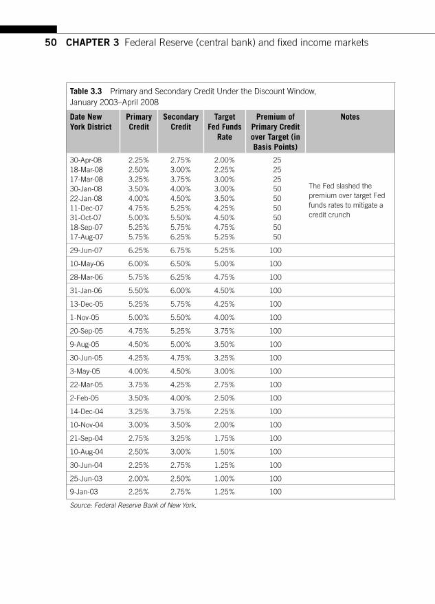
50 CHAPTER 3 Federal Reserve (central bank) and fi xed income markets
Table 3.3 Primary and Secondary Credit Under the Discount Window, January 2003 –April 2008
Date New York District
Primary Credit
Secondary Credit
Target Fed Funds
Rate
Premium of Primary Credit over Target (in Basis Points)
Notes
30-Apr-08 18-Mar-08 17-Mar-08 30-Jan-08 22-Jan-08 11-Dec-07 31-Oct-07 18-Sep-07
2.25% 2.50% 3.25% 3.50% 4.00% 4.75% 5.00% 5.25%
2.75% 3.00% 3.75% 4.00% 4.50% 5.25% 5.50% 5.75%
2.00% 2.25% 3.00% 3.00% 3.50% 4.25% 4.50% 4.75%
25 25 25 50 50 50 50 50
The Fed slashed the premium over target Fed funds rates to mitigate a credit crunch
17-Aug-07 5.75% 6.25% 5.25% 50
29-Jun-07 6.25% 6.75% 5.25% 100
10-May-06 6.00% 6.50% 5.00% 100
28-Mar-06 5.75% 6.25% 4.75% 100
31-Jan-06 5.50% 6.00% 4.50% 100
13-Dec-05 5.25% 5.75% 4.25% 100
1-Nov-05 5.00% 5.50% 4.00% 100
20-Sep-05 4.75% 5.25% 3.75% 100
9-Aug-05 4.50% 5.00% 3.50% 100
30-Jun-05 4.25% 4.75% 3.25% 100
3-May-05 4.00% 4.50% 3.00% 100
22-Mar-05 3.75% 4.25% 2.75% 100
2-Feb-05 3.50% 4.00% 2.50% 100
14-Dec-04 3.25% 3.75% 2.25% 100
10-Nov-04 3.00% 3.50% 2.00% 100
21-Sep-04 2.75% 3.25% 1.75% 100
10-Aug-04 2.50% 3.00% 1.50% 100
30-Jun-04 2.25% 2.75% 1.25% 100
25-Jun-03 2.00% 2.50% 1.00% 100
9-Jan-03 2.25% 2.75% 1.25% 100
Source: Federal Reserve Bank of New York.

51
level of reserves at the end of each two-week interval, or reserve maintenance period. Since they earn no interest on reserves, banks will try to minimize the amount of their excess reserves. The existence of a maintenance reserve period implies that the banks may make “last-minute” adjustments to make sure that their reserves comply with the requirements imposed on them by the Fed. This could in turn cause the Fed funds rate (the rate at which reserves may be borrowed) to exhibit some seasonality around the maintenance reserve period. Increasing the reserve requirements reduces the creation of credit and hence has the potential to reduce aggregate economic activity.
3.3 FED FUNDS RATES The Fed funds market is the market for the reserve balances at the Fed that must be maintained by depository institutions to meet the reserve requirements. The Fed does not pay interest on these reserves and, as a consequence, the depository institu-tions try to maintain the minimum amount of reserves necessary to conduct their activities. A depository institution that is short of reserves will borrow reserves from a bank that has a surplus in the Fed funds market. Such borrowing and lending can be done via two segments: either directly by the banks or through brokers.
Bartolini, Gudell, Hilton, and Schwarz (2005) analyze the Fed funds markets in detail and show that these two segments differ markedly in trading methods, price dynamics, and institutional participation. Usually, brokered transactions are of larger average size. Typically, big banks borrow reserves from smaller ones that have surplus reserves. Many of the depository institutions that have a surplus of reserves view the Fed funds market as a means of obtaining liquidity. Fed funds transactions typically take place overnight. Sometimes the Fed funds transactions extend over a term of a few days. It must be recognized that the Fed funds transactions are unsecured lend-ing and borrowing between depository institutions. The term Fed funds market is a lot less liquid than the overnight market. The relationship between the target Fed funds rate and the effective Fed funds rates is rather tight, except in period of crises or during the maintenance reserve requirements period.
3.3 FED funds rates
Table 3.4 Reserve Requirements
Type of Liability: Net Transaction Accounts
Requirement
Percentage of Liabilities Effective Date
$0 – 9.3 million 0 12-20-2007
More than $9.3 million to $43.9 million 3 12-20-2007
More than $43.9 million 10 12-20-2007
Source: Board of Governors of the Federal Reserve.

52 CHAPTER 3 Federal Reserve (central bank) and fi xed income markets
The target and the effective Fed funds rates are plotted in Figure 3.1 for the period 2000 –2008. As noted earlier, the target Fed funds rate is announced by the Fed based on its analysis of the economy. The effective Fed funds rate is the volume-weighted Fed funds rates at which reserves are lent and borrowed in reality. The Fed funds rate is a barometer of the activities of the depository institutions and refl ects the rate at which banks are able to obtain reserves. The supply and demand in the market for reserves determine the Fed funds rate. The rates go up when the demand for reserves is great and go down when the demand is sluggish. The central bank sets a target Fed funds rate. This target rate is a way for the central bank to signal the cost of credit. A cut in the target rate is viewed as easing credit, and an increase in the target rate is viewed as tightening credit availability. We can see from the fi gure that the period 2000 –2003 was one of signifi cant easing of credit, since the target Fed funds rate was cut from a high of 6.5% in July 2000 to a low of 1% until June 2004. During the period July 2004 to September 2007, the Fed was tight-ening credit by increasing the target rate from 1% to 5.25%.
The actual effective Fed funds rate will fl uctuate in the market, refl ecting market conditions. The central bank will pursue its open market policies to keep the actual Fed funds rate close to the target. When market conditions warrant a change in the target rate, the central bank will change it. Changes in the target Fed funds rate are made in FOMC meetings.
For fi nancial market stability purposes, the Fed may deviate from its planned mon-etary policy if the market circumstances warrant it. For example, the Fed cut the tar-get rate three times in 1998, largely to provide liquidity to a market that was rocked
0.51
1.52
2.53
3.54
4.55
5.56
6.57
5/16/00 9/28/01 2/10/03 6/24/04 11/6/05 3/21/07 8/2/082000–2008
Effective Target
FIGURE 3.1
Target and Effective Fed Funds Rates, May 16, 2000 –August 2, 2008 Source: Board of Governors of the Federal Reserve.

53
by the Russian default and hedge fund failures. The goal of these rate cuts was to ensure fi nancial stability. In 1999 and 2000, the Fed tended to tighten credit to keep infl ation under control in a rapidly expanding economy. Following the September 11, 2001, attacks on the World Trade Center, the Fed allowed the effective Fed funds rate to fall well below the target (see Figure 3.1 ) . From time to time, especially around the end of the calendar year, the Fed fund rates go up, resulting in the spikes evident in Figure 3.1 . This may be because many big depository institutions drive up the Fed funds rates seasonally.
3.4 PAYMENTS SYSTEMS AND CONDUCT OF AUCTIONS The Fed, acting as a fi scal agent for the Treasury, conducts the auctions of new Treasury securities. This entails collecting and processing competitive and noncom-petitive bids from dealers. These auctions are considered in detail in Chapter 5.
T-bills, T-notes, and T-bonds are issued in book-entry form. This is a tiered custodial system. This system records the ownership of securities in entries on the books of a series of custodians. This system begins with the Treasury and extends through the Federal Reserve Banks, depository institutions, brokers, and dealers to the ultimate owner. The tiered system operates as follows: The Treasury’s book-entry will estab-lish the total amount of each issue that is outstanding and the share of each that is held by each Federal Reserve Bank. Each Federal Reserve Bank will record how much of each issue is held by the depository institutions in its district that maintain book-entry accounts with it. The record of each depository institution will establish the amount that is held in its Reserve Bank for other depository institutions that do not maintain accounts at the Fed and for others.
Interest payments, as well as principal payments at maturity, are made by the Treasury, crediting the funds down the custodial tiers just described. Only certain depository institutions may have book-entry accounts at Federal Reserve Banks. Others must have their holdings refl ected on the books of a depository institution that, in turn, has holdings through a depository institution. Transfers are made by making appropriate entries. If the transfer of a security takes place within the juris-diction of a Federal Reserve Bank, no entries will be made at the Fed level or above. All entries will take place below the level of that Federal Reserve Bank.
3.5 FED’S ACTIONS TO STEM THE CREDIT CRUNCH OF 2007 – 2008 The ability of the Fed to supply enough reserves and maintain its desired objectives depends crucially on how well the money markets function. Under normal circum-stances, banks in the interbank markets will redistribute the reserves provided by the Fed. An interbank market is where banks lend to and borrow from each other. In addition, if banks and fi rms are able to access short-term funding in money markets
3.5 FED’s actions to stem the credit crunch of 2007 – 2008

54 CHAPTER 3 Federal Reserve (central bank) and fi xed income markets
by the issuance of commercial paper, the redistribution becomes very effective as these markets provide the necessary channels for liquidity provision and utilization. In late summer 2007 the mortgage market, especially in the subprime sector, began to experience a breakdown. This caused many banks to take write-downs in their mortgage-related positions and shore up their capital and liquidity by issuing equity and preferred stock and by curtailing lending. In addition, banks sharply curtailed their activity in the interbank markets because they were not sure about the extent of sub-prime exposure of other participating banks. The potential for counter-party default was perceived to be high. This caused the interest rates in the interbank markets to dramatically increase relative to the target Fed funds rates as shown in Figure 3.2 . The vertical lines correspond to actions taken by the Fed. Until the beginning of August 2007, one-month LIBOR was just about seven basis points higher than the target rate and was fairly stable. On August 14, 2007, the spread had increased to 35 basis points.
The Fed implemented several actions to stabilize the markets. These actions included the following:
As early as August 10, 2007, the Fed acknowledged that banks were experi -encing unusual funding needs as a result of dislocations in money and credit markets and said it would provide funds as needed. When this move failed to calm matters, the Fed followed up with a cut in the discount rate by 50 basis points on August 17, 2007, making the borrowing at the discount window only 50 basis points more expensive than the Fed funds rates. During the course of the crisis, the Fed cut the target Fed funds rates from a level of 5.25% in late August 2007 to a level of 2% by April 2008 in a sequence of moves shown in Table 3.5 . All the rate cuts were decided during scheduled FOMC meetings except the cut of 75 basis points, which was approved in an unscheduled meeting of FOMC on January 22, 2007 (following a major stock market downturn). The 75 basis points cut on March 18, 2008,
LIBOR behavior in credit crunch
2.00
2.50
3.00
3.50
4.00
4.50
5.00
5.50
6.00
May-07 Jul-07 Sep-07 Oct-07 Dec-07 Feb-08 Mar-08 May-08 Jul-08
LIBOR Target fed funds rate
FIGURE 3.2
LIBOR versus Target Fed Funds Rate During a Credit Crunch, May 2007 –July 2008

553.5 FED’s actions to stem the credit crunch of 2007 – 2008
Table 3.5 Fed Target Rate Cuts During the Credit Crunch
Fed’s Action Date Target Fed Funds Rate
September 18, 2007 5.25%
November 1, 2007 4.75%
December 11, 2007 4.50%
January 22, 2008 3.50%
January 30, 2008 3.00%
March 18, 2008 2.25%
April 03, 2008 2.00%
followed the meltdown of the two hedge funds managed by Bear Stearns. Earlier, on March 16, 2007, the Fed had met and coordinated a takeover of Bear Stearns by J. P. Morgan by guaranteeing the debt of Bear Stearns. In addition, it slashed the dis-count rate by another 25 basis points. The Fed authorized J. P. Morgan Chase to bor-row at the discount window on behalf of Bear Stearns, which was an emergency move last used in the Great Depression.
The Fed also announced a new lending program to provide credit to other big Wall Street fi rms and increased the maximum maturity of discount rate loans to 90 days from 30 days.
These actions failed to reduce the elevated levels of funding rates for short-term borrowing in the interbank markets, as is evident from Figure 3.2 . The Fed there-fore decided to initiate several term lending facilities. A clear description of these facilities can be found in Armantier, Krieger, and McAndrews (2008). An important term lending facility, known as the term auction facility (TAF), was created whereby banks were able to borrow from the Fed for a term of approximately one month by posting a broad menu of collateral, including mortgage-related collateral for which there were few takers in the private markets.
Evidence suggests that the TAF resulted in some relief in the interbank lending markets, especially when they were announced. The European Central Bank (ECB) also conducted similar auctions. The LIBOR spreads over the target rates are plotted in Figure 3.3 to help gauge the reaction of interbank spreads to the Fed’s actions. Note that the spreads have once again widened to over 40 basis points as of June 2008, suggesting that there are unresolved issues in the interbank markets.
These actions of the Fed come with some costs: Banks and other fi nancial institu-tions may interpret the Fed’s actions as a signal that the Fed will come to their res-cue in troubled times. This may encourage them to take greater risks in future. This is the risk of a “moral hazard. ” In addition, there is evidence that suggests that banks have designed structured credit products for the explicit purpose of posting them as collateral to the central bank to access credit. It is reasonable to suggest that the central banks, notably the Fed and the ECB, are now holding collateral that are very

56 CHAPTER 3 Federal Reserve (central bank) and fi xed income markets
diffi cult to value and for which a reliable market price simply does not exist in sec-ondary markets.
These actions of the Fed during a credit crunch shows that the stability and orderly functioning of the fi nancial markets may take priority over the often-cited objectives of maintaining orderly growth with price stability. Such actions attempt to balance the need to maintain well-functioning fi nancial markets with the risk of a moral hazard that promotes even more risk-taking behavior in future.
SUGGESTED READINGS AND REFERENCES Armantier , O. , Krieger , S., & McAndrews , J. ( 2008, 5 May ) . The term auction facility : Federal Reserve
Bank of New York .
Bartolini , L., Gudell , S., Hilton , S. , & Schwarz , K. ( 2005, November ) . Intraday trading in the overnight federal funds market . Current Issues in Economics and Finance , 11 ( 11) , 1 – 7 .
�40
�20
0
20
40
60
80
100
May-07 Jul-07 Sep-07 Oct-07 Dec-07 Feb-08 Mar-08 May-08 Jul-08
Credit crunch period
Spr
ead
in b
asis
poi
nts
FIGURE 3.3
LIBOR Spreads over Target Fed Funds Rates

57
CHAPTER
Fixed Income Markets and Their DerivativesCopyright 2009 by Academic Press. Inc. All rights of reproduction in any form reserved.
CHAPTER SUMMARY This chapter describes the organization and conduct of fi xed income markets. The over-the-counter market structure, which dominates the fi xed income markets, is explained. The role of primary dealers, interdealer brokers, and other intermediaries are described. The concept of pretrade and post-trade transparency are presented. The coexistence of voice-based trading and electronic (anonymous) trading is explained. We also compare the transparency of secondary markets in various sectors of the fi xed income markets and describe some recent developments in this area.
4.1 INTRODUCTION Fixed income markets are organized as over-the-counter (OTC) markets in the United States, in sharp contrast to stocks, which are predominantly traded in centralized or organized exchanges such as NYSE. Dealers act as market makers by purchasing the debt securities from borrowers (issuers) such as the U.S. Treasury and corporations and then sell the securities to investors such as pension funds, insurance companies, and the like. This process occurs in primary markets. Once the securities are issued, they trade in secondary markets, where the ownership of these securities merely exchanges hands without generating new capital or funds. Most of the trading in secondary markets occurs through the OTC structure. We fi rst describe the primary markets in fi xed income markets. The role of primary dealers is explained in this con-text. We also briefl y describe the primary market activities in corporate debt markets. This is followed by a description of secondary markets in the fi xed income sector. Here we explain the role played by interdealer brokers. Market transparency issues in the context of secondary markets are then presented. The fi nal section describes some of the latest developments in secondary markets.
Organization and transparency of fi xed income markets 4

58 CHAPTER 4 Organization and transparency of fi xed income markets
4.2 PRIMARY MARKETS The primary markets vary from one market to another. The major difference is the following: In Treasury debt markets, dealers bid in auctions conducted by the Fed, which acts on behalf of the Treasury, to obtain the Treasury debt securities in the pri-mary markets. Similar auctions have been used to sell Federal agency debt securities. In all other debt markets, dealers underwrite by forming syndicates to eventually dis-tribute the securities to investors. In both auction mechanisms (used in the Treasury market and the agency market) and in the underwritten offerings, dealers have to perform several functions, including (a) assessing the demand for the debt issue, (b) pricing the issue, (c) hedging inventory positions, and (d) distributing securities to ultimate investors. These are critical functions performed by the dealer community.
4.2.1 Treasury markets
In Treasury markets, primary markets are characterized by an important set of play-ers known as primary dealers. They are banks and securities brokerages that trade in U.S. Government securities with the Federal Reserve System. They have a direct phone line with the Fed and participate in the open market operations. Primary deal-ers ’ daily average trading volume in fi xed income markets during the fi rst week of June 2008 exceeded $1 trillion, of which trading in U.S. Government securities was in excess of $500 billion.
Bank-related primary dealers must be in compliance with Tier I and Tier II capital standards under the Basel Capital Accord, with at least $100 million of Tier I cap-ital. Registered broker-dealers must have at least $50 million in regulatory capital. Primary dealers are expected to participate meaningfully in both the Fed’s open market operations and Treasury auctions and to provide the Fed’s trading desk with market information and analysis that are helpful in the formulation and implementa-tion of monetary policy. Currently there are 20 primary dealers, as listed in Table 4.1 .
4.2.2 Corporate debt
Corporate bonds can be placed in public bond markets by registering with the Securities and Exchange Commission (SEC). The underwriters typically use a “fi rm commitment ’’ contract to distribute the debt securities to various institu-tional buyers. In some circumstances, the underwriters use “best efforts ’’ distribu-tion. Corporate bonds can also be privately placed to a few institutional investors such as pension funds and insurance companies. 1 Or corporate bonds can be sold through Rule 144a to qualifi ed institutional buyers (QIBs), without registration and with signifi cant trading restrictions until they are subsequently registered. Rule 144a, adopted by the SEC in April 1990, allows for an exemption from registration for
1 See “The Economics of the Private Placement Market,” by Mark Carey, Stephen Prowse, John Rea, and Gregory Udell, Staff, Board of Governors, December 1993.

59
primary market transactions, provided that the buyer is a sophisticated fi nancial insti-tution and defi ned as a QIB, as before. In this context, QIBs are fi nancial institutions, corporations, and partnerships that own and invest on a discretionary basis $100 mil-lion or more of securities. By and large, Rule 144a issues are more important for “ high-yield” issues and less signifi cant for “investment-grade ” issues.
4.3 INTERDEALER BROKERS The inner market in the government securities market comprises the interdealer brokers (IDBs). Interdealer brokers aggregate information about the bids and offers posted by various dealers and disseminate that information on computer screens. They do so without revealing the identities of the dealers. This enables the deal-ers to undertake their proprietary trading activities anonymously. Dealers pay the interdealer brokers commissions for this service. Major interdealer brokers include Cantor Fitzgerald (eSpeed is their electronic trading platform), ICAP (Garban), Liberty, and so on. IDBs provide access typically only to primary dealers. In 1991, a real-time price and quote distribution system known as GOVPX that disseminates information about the Treasury market around the clock was established. It showed all the executed trades, best bids, and offers. Since then, electronic trading platforms have become rather common for trading newly issued Treasury debt securities.
4.3 Interdealer brokers
Table 4.1 Primary Dealers as of December 2007
BNP Paribas Securities Corp. Banc of America Securities LLC Barclays Capital Inc. Bear, Stearns & Co., Inc. Cantor Fitzgerald & Co. Citigroup Global Markets Inc. Countrywide Securities Corporation Credit Suisse Securities (USA) LLC Daiwa Securities America Inc. Deutsche Bank Securities Inc. Dresdner Kleinwort Securities LLC Goldman, Sachs & Co. Greenwich Capital Markets, Inc. HSBC Securities (USA) Inc. J. P. Morgan Securities Inc. Lehman Brothers Inc. Merrill Lynch Government Securities Inc. Mizuho Securities USA Inc. Morgan Stanley & Co., Inc. UBS Securities LLC
Source: Federal Reserve Bank of New York.

60 CHAPTER 4 Organization and transparency of fi xed income markets
The primary dealers rely on the interdealer brokers for a signifi cant percentage of their trades, as noted in Table 4.2 .
Note from Table 4.2 that IDBs account for nearly 50% of trading in Treasury debt securities, whereas they contribute to less than 1% of trading in corporate bond mar-kets and less than 2% of trading in agency markets. In MBS markets they account for about 25% of all trades.
The interdealer broker market has become quite competitive over the last few years. The interdealer brokers provide liquidity for dealers. For this service, they enjoy a commission and a spread. The entry of Liberty Brokerage further eroded the profi tability of interdealer brokers. This is because the dealers (who helped set up Liberty) wanted to lower the costs of trading in the interdealer broker markets.
Several IDBs have since set up electronic platforms for buying and selling gov-ernment bonds. Cantor Fitzgerald’s e-Speed started executing electronic bond trades from early 1999, and now there are many IDB electronic screens, which execute gov-ernment bond trades with live quotes. They include Garban (ICAP), which is a major IDB. In electronic trading there is no human intervention, and costs are much lower as a consequence. Newly issued Treasury securities trade every 10 to 20 seconds in IDB market. 2 In addition to electronic trading there is a voice-based trading with human intervention as well. Together, for Treasury markets, a number of trading plat-forms and IDBs provide live quotes.
4.4 SECONDARY MARKETS Secondary markets provide the venue where ownership of seasoned (already issued) debt securities exchanges hands from one institutional or noninstitutional customer to another. As noted earlier, the predominant form of trading in both Treasury and corporate bonds issued by domestic companies occurs in dealer markets or OTC mar-kets, in which dealers participate. These are sometimes referred to as the multid ealermarket. A very small fraction of the trading also occurs in organized exchanges such
2Michael Barclay, Terence Hendershott, and Kenneth Kotz, “Automation versus Intermediation: Evidence from Treasuries Going Off the Run,” Journal of Finance, Vol. LXI, No. 5, October 2006.
Table 4.2 Primary Dealer Transactions with IDBs and Customers, Week Ending June 25, 2008 (Daily Average Figures; in Millions of Dollars)
U.S. Government Securities
Agency and GSE (Excluding MBS) MBS Corporate Debt
With IDBs 220,684 With IDBs 7,031 With IDBs 51,290 With IDBs 648
With others 279,632 With others 101,577 With others 146,006 With others 193,472
Total 500,516 Total 108,608 Total 197,296 Total 194,120
Source: Federal Reserve.

61
as the New York Stock Exchange (NYSE), the American Stock Exchange (AMEX), and some foreign exchanges. By and large, institutional trading activity in Treasury debt and corporate bonds tends to occur in OTC markets. Trades that occur in the NYSE’s automated bond trading system (ABS) tend to be made by retail investors.
4.4.1 Dealer market transparency
Transparency of a market can be defi ned as “the widespread availability of infor-mation relative to current opportunities to trade and recently completed trades. ” 3 Transparency is classifi ed into pretrade transparency and post-trade transparency.Pretrade information includes (a) fi rm (live) bid prices and (live) offer prices and the quantities that the market maker is willing to transact, which enable the investors to know the prices at which specifi ed quantities of bonds can be bought or sold; and (b) in multiple dealer markets (as in corporate bonds), pretrade transparency infor-mation will require the consolidation of bid prices and offer prices as well as the quantities associated with those prices across all market makers (or as many mar-ket makers or dealers as possible); existence of effective consolidation mechanisms serves to reduce the search costs to potential investors by providing them, in one screen, with a complete picture of trading opportunities, not with just one dealer but with multiple dealers. This, in turn, promotes overall transparency.
Relevant post-trade information includes the prices and the volume of all indi-vidual transactions that have actually taken place in the market at the time a poten-tial investor is contemplating a trade. Post-trade transparency of a market determines the information that investors will have about most recent trades and will help them evaluate the quality of execution of trades relative to recently concluded trades. Once again, existence of effective consolidation mechanisms serves to reduce the search costs to potential investors by providing them with a complete picture of recently completed buy and sell orders with various dealers and the quality of trade execution. In a market where the pretrade and post-trade transparency is poor, infor-mation about the prevailing buying interest or prevailing selling interest or quality of recently completed trade executions is costly and time-consuming to acquire. As a result, prices will not effi ciently refl ect all the buying and selling interests that are present in the market. This may lead to poor trade execution; investors may receive or pay prices that are not necessarily the best available prices in the market.
4.4.2 Indicators of transparency
Extensive trading activity in the secondary markets (number of trades and volume of trading), narrow bid-offer spreads, and willingness to trade greater quantities (at a given bid or offer) provide valuable signals about the true value of the security and help make the market more transparent. In a market where trading activity is poor,
4.4 Secondary markets
3International Organization of Securities Commissions: IOSCO Objectives and Principles of Securities Regulation.
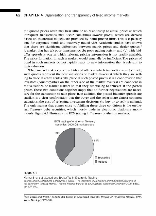
62 CHAPTER 4 Organization and transparency of fi xed income markets
the quoted prices often may bear little or no relationship to actual prices at which infrequent transactions may occur. Sometimes matrix prices, which are derived based on theoretical models, are provided by bond pricing fi rms. This is especially true for corporate bonds and inactively traded ABSs. Academic studies have shown that there are signifi cant differences between matrix prices and dealer quotes. 4 A market that has (a) poor transparency, (b) poor trading activity, and (c) wide bid-offer spreads is one in which relevant pricing information is not readily available. The price formation in such a market would generally be ineffi cient: The prices of bond in such markets do not rapidly react to new information that is relevant to their valuation.
When market makers post live bids and offers at which transactions can be made, such quotes represent the best valuations of market makers at which they are will-ing to trade. If active trades take place at such posted prices, it is a confi rmation that investors (counterparties on the other side of the market makers) are confi dent in the valuations of market makers so that they are willing to transact at the posted prices. These two conditions together imply that no further negotiations are neces-sary for the transaction to take place. If, in addition, the posted bid-offer spreads are small, it is a clear confi rmation that the buyer and the seller share almost common valuations; the cost of reversing investment decisions (to buy or to sell) is minimal. The only market that comes close to fulfi lling these three conditions is the on-the-run Treasury debt securities, which mostly trade in electronic platforms anony-mously. Figure 4.1 illustrates the ECN trading in Treasury on-the-run markets.
39%
61%
BrokerTec
eSpeed
ECN trading of on-the-run Treasurysecurities, 2005:Q3 market share
FIGURE 4.1
Market Share of eSpeed and BrokerTec in Electronic Trading Source: Bruce Mizrach and Christopher J. Neely, “The Transition to Electronic Communications Networks in the Secondary Treasury Market, ” Federal Reserve Bank of St. Louis Review , November/December 2006, 88 (6), pp. 527 –541.
4 See Warga and Welch, “Bondholder Losses in Leveraged Buyouts,” Review of Financial Studies, 1993, Vol. 6, No. 4, pp. 959–982.

63
BrokerTec has now been taken over by ICAP, which is the largest ECN in North America. Similar ECNs operate in Europe and other areas.
4.4.3 Evidence on trading characteristics
Fleming (2003), in a study of the Treasury debt securities during the period from December 30, 1996, to March 31, 2000, showed that the mean trading volume of 2-, 5-, and 10-year U.S. Treasury securities ranged from $3.81 billion to $6.65 billion per day. 5 The mean number of trades per day ranged from 467 to 693. The mean bid-offer spreads for the same Treasury securities ranged from 0.21 to 0.78 of 1/32 nds. These are very narrow bid-offer spreads indicating a very liquid and (when combined with the large trading volume) transparent market. To summarize, Treasury benchmark bonds and notes trade in a market where the measures of market transparency are extremely high. In a recent study of transactions data, researchers found that in the corporate bond markets, the mean number of trades (based on 6.6 million trades in over 16,700 corporate bonds) is less than two. 6 The dollar trading volume averages about $0.16 million, and the average frequency of days with a trade is 33%. As noted in Chapter 1, Table 1.5, whereas the new issue volume of corporate bonds in the overall domestic debt markets is about 14% of the entire market, the proportion of trading that occurs in corporate bond markets in the secondary markets is just 2% of the trading volume in secondary markets for debt securities. In sharp contrast, more than 60% of the secondary market trading volume is accounted for by Treasury secu-rities, even though the share of new issue volume of Treasuries is very similar to that of the corporate bond sector. Other studies also point to extreme lack of trading in corporate bonds markets. For example, of the nearly 400,000 corporate bond issues outstanding in 1996, only 4% were traded at least once during the entire year. 7
A recent study examined the bid-offer spreads of corporate and Treasury bonds using a sample that consisted of 150,000 transactions in corporate bonds and 55,000 transactions in government bonds in the OTC market during the period 1995 to 1997. The authors of this study concluded that the spreads for corporate bonds are twice as high for government bonds. 8
Thus, evidence summarized in this section suggests that Treasury on-the-run issues tend to exhibit excellent pretrade and post-trade transparency. Corporate debt mar-kets seem to have very poor transparency. As Biais and Green (2005) observe in the context of corporate debt: “The OTC markets are decentralized and dealer-intermediated.
4.4 Secondary markets
5 Michael J. Fleming, “Measuring Treasury Market Liquidity,” Federal Reserve Bank of New York Economic Policy Review, September 2003, pages 83–108.6 A. Edwards, L. Harris, and M. Piwowar, “Corporate Bond Market Transparency and Transaction Costs,’’ SEC working paper, 2004.7 Endo, Tadashi, “Linkage of Corporate Bond Market to Government Bond Market,’’ World Bank, 2001.8 Sugato Chakravarty and Asani Sarkar, “Liquidity in U.S. Fixed Income Markets: A Comparison of the Bid-Ask Spreads in Corporate, Government and Municipal Bond Markets,” staff report 73, Federal Reserve Bank of New York, 1999.

64 CHAPTER 4 Organization and transparency of fi xed income markets
There is little pretrade transparency, as dealers do not post widely disseminated fi rm quotes. Post-trade transparency is also quite limited, although it has recently improved under pressure from Congress, the SEC, buy-side traders, and the NASD. Only dealers can post quotes, and thus investors cannot compete to supply liquidity. ” The opacity (or lack of transparency) of corporate bond markets has been a matter of concern to Congress and the SEC for a number of years. Congress held hearings in 1998 on the lack of readily available pricing information in corporate bond markets. The SEC has been long concerned with the lack of routine access to transaction information for the broad universe of corporate bonds and consequently its inability to conduct rou-tine surveillance of trading in corporate bond markets.
4.4.4 Matrix prices and execution costs
Since the trading activity in corporate bonds is sporadic, accurate data on corporate bond prices are very diffi cult to get. Two sources of price quotes are (a) exchanges (such as the NYSE and the AMEX) and (b) OTC dealers. As noted earlier, exchange data are based on a very small percentage of the overall trading activity. OTC quotes of corporate bond prices are rough estimates of their true values, based on some models. Often models price a few active bonds and the rest of the bonds are priced via matrix prices by using some mathematical models and by simply adding some spreads. These prices can change over time because inputs to the model such as inter-est rates or spreads change over time. Such matrix prices or quotes are of limited help as relevant indicators of the true values. Additional work in this area shows sig-nifi cant differences between matrix prices and trader quotes and institutional data. 9 In sum, corporate bond markets exhibit (a) poor pricing and volume information, (b) lack of reliable bid-offer spreads, (c) low trading frequency and turnover, and (d) lack of impersonal trading.
4.5 EVOLUTION OF SECONDARY MARKETS A number of steps have been taken to improve the transparency of debt markets. Some of these are highlighted in Table 4.3 .
Since 2002, price transparency in corporate bond markets has started to improve. This is due to the initiative taken by the SEC, which prompted the National Association of Securities Dealers (NASD) to develop a central reporting system called the Trade Reporting and Compliance Engine (TRACE). TRACE has been imple-mented in phases and has slowly but steadily improved reporting of trades. As of now, a greater number of corporate bond trades are being reported to the market in a much shorter period of time following execution. Usually the time lag is less than a few minutes. Moreover, such transactions are also reported to screens such
9 Arthur Warga and Ivo Welch, “Corporate Bond Price Discrepancies in the Dealer and Exchange Markets,” Journal of Fixed Income, December 1991, pp. 7–16.

65
as Bloomberg. The coverage by TRACE is still somewhat limited; certain high-yield bonds and thinly traded corporate bonds are not frequently reported on TRACE.
The introduction of TRACE has renewed the interest of scholars and practitioners in the reexamination of the characteristics of the corporate bond markets. A paper by Bossembinder, Maxwell, and Venkataraman (2005) examined the extent to which the TRACE system has infl uenced the trade execution costs for corporate bonds. They look at a sample of institutional trades, both before and after the introduction of the TRACE system, and report the following conclusions: First, for bonds that are eligible for TRACE transaction reporting, the trade execution costs decline roughly 50%. More interestingly, they fi nd that the trade execution costs decline 20% even for bonds that are not eligible for TRACE reporting. Their conclusion that the corporate bond markets have become more competitive after TRACE implementation supports the previous evidence and research that the corporate bond markets, prior to the introduction of TRACE, was much less transparent.
Transparency in muni bond markets has also been improving over the years. In 1994 interdealer transactions were reported. This was followed in 1998, when deal-ers began reporting customer trades as well. The Municipal Securities Rulemaking Board (MSRB), which makes rules regulating dealers who deal in municipal bonds, municipal notes, and other municipal securities, began reporting next-day price information on both interdealer and customer transactions involving bonds that traded four or more times per day. In 2003, the MSRB began T � 1 reporting for municipal bond transactions and eliminated the requirement that required report-ing only bonds that traded four or more times per day. And, fi nally, a new MSRB rule (Rule G-14), scheduled to become effective in the beginning of 2005, required
4.5 Evolution of secondacy markets
Table 4.3 Initiatives to Improve Market Transparency
Year Initiatives Purpose
1991 GOVPX Provision of real-time trade price and volume information for U.S. Treasuries from the interdealer market.
1994 FIPS 50 NASD began publishing data on 50 high-yield bonds (most actively traded). Information provided consisted of daily high, low, and volume updated hourly, with summary closing information.
1995 – 2000 Municipal bond markets
In 1995, daily summary reports on relatively active bonds — that is, those that traded four or more times in a day — were provided. At the end of 1998 those summary reports were made available to the public, and by 2000 all trade data were published on a T � 1 basis. By 2007, trade data have been published with a delay of just 15 minutes.
2002 – 2008 TRACE Major initiative to signifi cantly improve the transparency of corporate bond markets.

66 CHAPTER 4 Organization and transparency of fi xed income markets
brokers and dealers to report transactions in municipal securities within 15 minutes of the time of trade. This rule became effective in July 1996.
SUGGESTED READINGS AND REFERENCES The following papers deal with issues of market transparency in detail. Some of the discussions in this chapter have relied upon these academic and policy papers.
Barclay , M. , Hendershott , T. , & Kotz , K. ( 2006, October ) .Automation versus intermediation: Evidence from treasuries going off the run . Journal of Finance , LXI ( 5) , 2395 – 2414 .
Carey , M. , Prowse , S. , Rea , J. , & Udell , G. ( 1993, December ) . The economics of the private placement market . Board of Governors .
Chakravarty , S., & Sarkar , A. ( 2003, June ) .Trading costs in three U.S. bond markets . Journal of Fixed Income , 13 ( 1) , 39 – 48 .
Edwards , A. , Harris , L. , & Piwowar , M. ( 2007, June ) . Corporate bond market transparency and trans-action costs . Journal of Finance , 62 ( 3) , 1421 – 1451 .
Endo , T. ( 2001) . Linkage of corporate bond market to government bond market. World Bank .
Fleming , M. ( 2003, September ) . Measuring treasury market liquidity , Federal Reserve Bank of New York . Economic Policy Review , 9 ( 3) , 83 – 108 .
Transparency of corporate bond markets, Report of the Technical Committee of the International Organization of Securities Commissions, www.iosco.org , May 2004.
Warga , A., & Welch , I. ( 1993) . Bondholder losses in leveraged buyouts . Review of Financial Studies , 6 ( 4) , 959 – 982 .

67
CHAPTER
Fixed Income Markets and Their DerivativesCopyright 2009 by Academic Press. Inc. All rights of reproduction in any form reserved.
CHAPTER SUMMARY This chapter defi nes repo and reverse repo agreements. Through worked-out exam-ples, the chapter illustrates how to fi nance long positions and establish short posi-tions in repo markets. Real-life features such as haircuts (margins) are treated. The differences between general collateral (GC) repo rates and special repo rates are explained. The relationship between GC repo rates and other short-term interest rates such as the effective Fed funds rate and one-month LIBOR are analyzed. The possibility of fails in repo markets and recent innovations in the repo markets are described.
5.1 REPO AND REVERSE REPO CONTRACTS Repurchase agreements, often simply referred to as repo agreements, are used by dealers to fi nance their positions and to hedge their market risk. They are also used by the central bank or the Fed to manage reserves and maintain the short-term inter-est rates closely aligned to the target Fed funds rate. This chapter describes the repo contracts and the market institutions and illustrates several applications.
5.1.1 Repo contract defi ned
A repo agreement is a contract in which a security is sold with an agreement on the initiation date to repurchase the security at a higher price on a later date specifi ed in the contract.
Financing debt securities: Repurchase (repo) agreements 5

68 CHAPTER 5 Financing debt securities: Repurchase (repo) agreements
Example 5.1 In Figure 5.1 , we illustrate a repo transaction. Institution X delivers a Treasury note with a mar-ket value of $1,000,000 to Institution Y, which delivers to Institution X $1,000,000 in cash (ini-tial transaction, or the opening leg in the fi gure). For simplicity, we assume that the Treasury note is selling at par. On the same day, Institution X agrees to buy back from Institution Y the same security on the very next day (overnight) at a price of $1,000,138.89 (closing transac-tion, which occurs the next day).
The price at which Institution X agrees to buy back was arrived at in this example so that the lender of cash (Institution Y) gets a rate of interest of 5%. Namely,
1 000 000 1 0 051
3601 000 138 89, , . , , . .� � � �
⎛⎝⎜⎜⎜⎜
⎞⎠⎟⎟⎟⎟
We have used the actual/360 convention in computing the repo costs, which is the repo market convention. This rate of interest, 5%, is known as the repo rate. In this example the term of the loan was overnight (one day), and the loan made by Institution Y to Institution X was collateralized by the Treasury note. This is important because the lender of cash can always sell the Treasury note if the borrower defaults on the repo contract. For this reason, we regard repo contracts as secured loans. In the example described in Figure 5.1 , Institution X
1. Initial Transaction in Repo Agreement(Opening leg—takes place at date t)
Treasury note
Institution X Institution Y
Cash $1,000,000
2. Closing Transaction in Repo Agreement(Closing leg—takes place at date t�1)
Treasury note
Institution X Institution Y
Cash $1,000,138.89
FIGURE 5.1
Example of a Repo Transaction (Opening and Closing Legs)

69
is said to have a repo position. It has effectively a long position in the Treasury note. To see why this is the case, note that the profi tability of Institution X goes up when the Treasury note price goes up. Institution X can buy the note at the contracted price of $1,000,138.89 and then sell the note at the higher prevailing market price.
We therefore interpret repo agreements as secured lending. Institution X posts the Treasury note as collateral and borrows cash from Institution Y, which holds the security simply as collateral. The next day, Institution X pays back the money borrowed plus the repo interest, and the collateral is returned to Institution X.
5.1.2 Reverse repo contract defi ned
A reverse repo agreement is a contract in which a security is borrowed with an agreement on the initiation date to replace the security at a higher price on a later date specifi ed in the contract.
Example 5.2 Figure 5.2 illustrates a reverse repo transaction from the perspective of Institution X. Institution X borrows a Treasury note with a market value of $1,000,000 to Institution Y and delivers to Institution Y $1,000,000 cash (initial transaction in the fi gure). For simplicity, we assume that the Treasury note is selling at par. On the same day, Institution X agrees to sell back to Institution Y the same security on the very next day at a price of $1,000,138.89 (closing trans-action, which occurs the next day).
The price at which Institution X agrees to sell back was arrived at in this example so that the lender of cash (Institution X) gets a rate of interest of 5%. Namely,
1 000 000 1 0 051
3601 000 138 89, , . , , . .� � � �
⎛⎝⎜⎜⎜
⎞⎠⎟⎟⎟⎟
This rate of interest, 5%, is known as the reverse repo rate. In this example the term of the loan was overnight (one day). Institution X, which borrowed the Treasury note from Institution Y, collateralizes its position by delivering cash. This is important because the lender of secu-rity can rely on cash if the borrower of security defaults on the repo contract. In the example described in Figure 5.2 , Institution X is said to have a reverse repo position. It has effectively a short position in the Treasury note. To see why this is the case, note that the profi tability of Institution X goes up when the Treasury note price goes down. Institution X can acquire the note at the lower prevailing market price and then sell the note at the contracted price of $1,000,138.89.
5.1 Repo and reverse repo contracts

70 CHAPTER 5 Financing debt securities: Repurchase (repo) agreements
5.1.3 Repo as secured lending
There is a conceptual relationship between the repo and reverse repo transac-tions on the one hand and secured lending and borrowing on the other. For exam-ple, a repo transaction is conceptually similar to posting a security as collateral and borrowing money at the repo rate. Likewise, a reverse repo transaction is conceptually similar to borrowing security and placing cash (possibly the proceeds of selling the bor-rowed security) as collateral. Throughout our discussions, we treat these contracts as secured lending and borrowing. In repo and reverse repo transactions, the ownership of the underlying security changes hands. In the secured lending (and borrowing) interpre-tation, the ownership does not change hands. This difference should be refl ected in the manner in which repo rates are calculated.
5.2 REAL-LIFE FEATURES This example of a repo contract is simplifi ed in many respects. First we have assumed that the lender of cash is willing to lend an amount equal to the market value of the Treasury note. In reality, the lender of cash will lend an amount that is slightly lower than the market value of the security delivered. The difference between the market value of the security posted and the cash lent is known as margin, or hair-cut. This amount may vary with the type of security delivered by the borrower of cash. Normal fl uctuations in the market value of the underlying collateral might sometimes lead to situations in which the money owed by the borrower may exceed
1. Initial Transaction in Reverse Repo Agreement(Opening leg—takes place at date t)
Treasury note
Institution X Institution Y
Cash $1,000,000
2. Closing Transaction in Reverse Repo Agreement(Closing leg—takes place at date t�1)
Treasury note
Institution X Institution Y
Cash $1,000,138.89
FIGURE 5.2
Example of a Reverse Repo Transaction (Opening and Closing Legs)
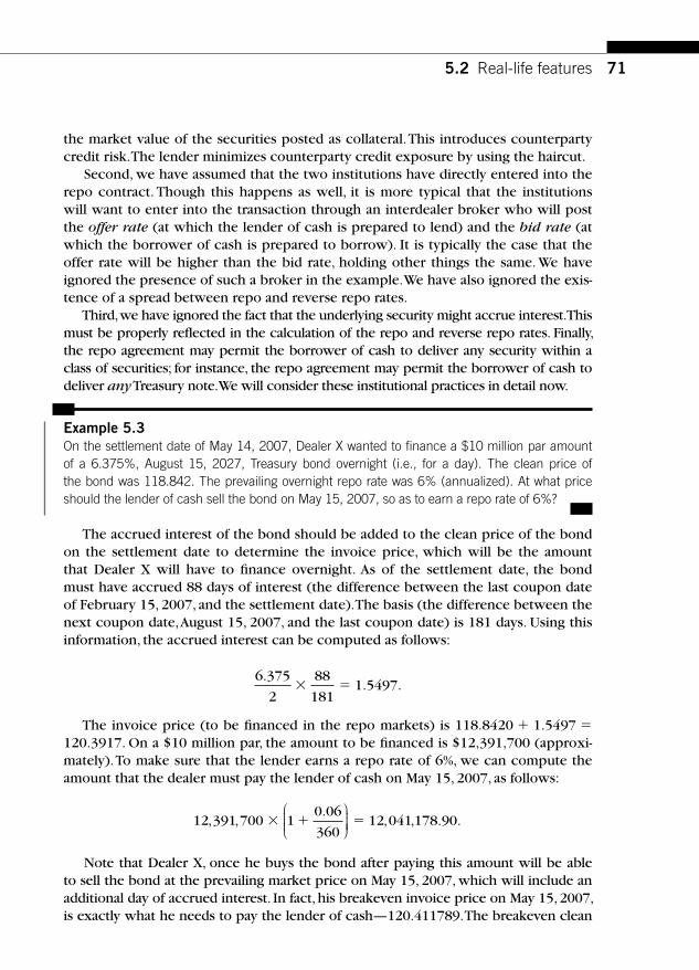
71
the market value of the securities posted as collateral. This introduces counterparty credit risk. The lender minimizes counterparty credit exposure by using the haircut.
Second, we have assumed that the two institutions have directly entered into the repo contract. Though this happens as well, it is more typical that the institutions will want to enter into the transaction through an interdealer broker who will post the offer rate (at which the lender of cash is prepared to lend) and the bid rate (at which the borrower of cash is prepared to borrow). It is typically the case that the offer rate will be higher than the bid rate, holding other things the same. We have ignored the presence of such a broker in the example. We have also ignored the exis-tence of a spread between repo and reverse repo rates.
Third, we have ignored the fact that the underlying security might accrue interest. This must be properly refl ected in the calculation of the repo and reverse repo rates. Finally, the repo agreement may permit the borrower of cash to deliver any security within a class of securities; for instance, the repo agreement may permit the borrower of cash to deliver any Treasury note. We will consider these institutional practices in detail now.
Example 5.3 On the settlement date of May 14, 2007, Dealer X wanted to fi nance a $10 million par amount of a 6.375%, August 15, 2027, Treasury bond overnight (i.e., for a day). The clean price of the bond was 118.842. The prevailing overnight repo rate was 6% (annualized). At what price should the lender of cash sell the bond on May 15, 2007, so as to earn a repo rate of 6%?
The accrued interest of the bond should be added to the clean price of the bond on the settlement date to determine the invoice price, which will be the amount that Dealer X will have to fi nance overnight. As of the settlement date, the bond must have accrued 88 days of interest (the difference between the last coupon date of February 15, 2007, and the settlement date). The basis (the difference between the next coupon date, August 15, 2007, and the last coupon date) is 181 days. Using this information, the accrued interest can be computed as follows:
6.. .
375
2
88
1811 5497� �
The invoice price (to be fi nanced in the repo markets) is 118.8420 � 1.5497 � 120.3917. On a $10 million par, the amount to be fi nanced is $12,391,700 (approxi-mately). To make sure that the lender earns a repo rate of 6%, we can compute the amount that the dealer must pay the lender of cash on May 15, 2007, as follows:
12 391 700 10 06
36012 041 178 90, ,
., , . .� � �
⎛⎝⎜⎜⎜
⎞⎠⎟⎟⎟⎟
Note that Dealer X, once he buys the bond after paying this amount will be able to sell the bond at the prevailing market price on May 15, 2007, which will include an additional day of accrued interest. In fact, his breakeven invoice price on May 15, 2007, is exactly what he needs to pay the lender of cash —120.411789. The breakeven clean
5.2 Real-life features

72 CHAPTER 5 Financing debt securities: Repurchase (repo) agreements
price will be 120.411789 less the accrued interest on May 15, 2007. The accrued inter-est on May 15, 2007, is 1.5673, which leads to a breakeven clean price of 118.8445.
Using repo rates of various maturities, we can compute their breakeven prices, which are in fact the forward prices at which the bond can be sold to break even.
Example 5.4 On August 31, 2007, the 30-year T-bond with a coupon of 5.00% and maturing on May 15, 2037, was quoted at a clean price of 102.50. The general collateral repo rate for a term of one month was 4.775%. A bond dealer receives an order from a client to buy this bond forward in one month’s time. What is the forward price that dealer should quote? Why? How should the dealer hedge the exposure, assuming that the deal is done on August 31, 2007?
The dealer will fi rst compute the forward price as follows:
1. Borrow cash to buy the bond in the repo markets for a one-month term on August 31, 2007.
2. Figure out how much has to be paid in the repo markets on September 30, 2007, to retrieve the collateral.
3. This is the forward price at which the dealers will break even. Any additional profi t mar-gin would depend on the extent of competition.
Figure 5.3 shows the computation of one-month forward price for this T-bond. The dealer will sell forward (on August 31, 2007) to the client at a forward price of
8
9
10
11
12
13
14
15
16
17
18
19
20
21
22
23
24
25
C D E F G H I
Settlement date 8/31/07
Benchmark Coupon MD YTM PCD NCD Days
Accrued
Thirty-year 5.00% 5/15/37 4.84% 05/15/07 11/15/07 108
Accrued Clean-price Dirty price
1.4674 102.5000 103.96741
Repo Rate 4.775%
Term 9/30/07
# days 30 � F8-E8
Money to be borrowed on 8/31/07 103.96741 � E15
Money to be repaid on 9/30/07 104.38111 � E15*(1�F19/360*F17)
Accrued on 9/30/2007 1.8750 � (F18-G11)/(H11-G11)*D11/2*100
Quoted Forward Price 102.5061 � F21�F22
Note that the quoted forward price is less than the current price of the bond, due to positive carry.
FIGURE 5.3
Forward Price on Bonds Using Repo Markets

73
102.5061 and simultaneously repo out the (go long) bond at a term repo of 4.775% for one month.
On September 30, 2007, the dealer will pay 104.38111 to the lender in the repo markets and collect the bond and deliver it to the client. The client will pay the quoted forward price of 102.5061 plus the accrued interest of 1.8750 on September 30, 2007.
In the next example, we take into account the practice of haircuts in computing the profi ts and losses associated with repo transactions.
Example 5.5 On June 10, 1986, Dealer X wanted to fi nance $10 million par amount of a 7.25%, May 15, 2016, T-bond. The dealer wanted to carry the position until June 13, 1986. Given the historical data in Table 5.1 , what is the profi t or loss associated with this trade? Assume a haircut of 0.5%.
Let’s examine this trade. Table 5.1 gives the prices in the market during the relevant period. (The prices are given in decimals.)
On June 10, 1986, Dealer X bought the T-bond and delivered it to the repo dealer. The repo dealer accepted the T-bond as a collateral and lent cash at the repo rate. Typically, a repo dealer would not lend cash equal to the market price of the T-bond. We can compute the fi nancing cash fl ows as follows: First we can compute the invoice prices of the security by adding accrued interest to the clean prices pre-sented in Table 5.2 .
1. Amount to be borrowed. The dealer bought the T-bond. Since the dealer bought the bond on June 10, 1986, he paid 94.16 plus accrued interest. The fl at price of the T-bond was 94.16, the accrued interest was 0.51223; hence, the full price was 94.67. On $10 million par, the full (invoice) price was approximately 9,467,222.83. (The mechanics of calculating accrued interest are described in Chapter 2.)
2. Haircut . The haircut taken by the repo dealer was 0.5% of market value:
0 51
1009 467 222 83 47 336 11. , , . $ , .� � �
5.2 Real-life features
Table 5.1 Clean Price History
Date Price
6/10/1986 94.16
6/11/1986 94.97
6/12/1986 95.03
6/13/1986 96.78
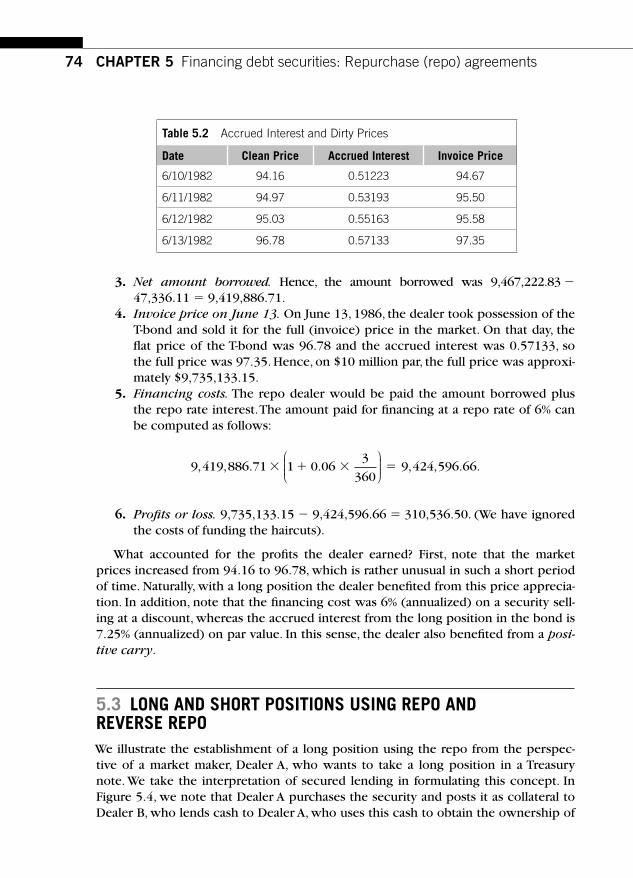
74 CHAPTER 5 Financing debt securities: Repurchase (repo) agreements
3. Net amount borrowed. Hence, the amount borrowed was 9,467,222.83 � 47,336.11 � 9,419,886.71.
4. Invoice price on June 13. On June 13, 1986, the dealer took possession of the T-bond and sold it for the full (invoice) price in the market. On that day, the fl at price of the T-bond was 96.78 and the accrued interest was 0.57133, so the full price was 97.35. Hence, on $10 million par, the full price was approxi-mately $9,735,133.15.
5. Financing costs. The repo dealer would be paid the amount borrowed plus the repo rate interest. The amount paid for fi nancing at a repo rate of 6% can be computed as follows:
9 419 886 71 1 0 063
3609 424 596 66, , . . , , . .� � � �
⎛⎝⎜⎜⎜
⎞⎠⎟⎟⎟
6. Profi ts or loss. 9,735,133.15 � 9,424,596.66 � 310,536.50. (We have ignored the costs of funding the haircuts).
What accounted for the profi ts the dealer earned? First, note that the market prices increased from 94.16 to 96.78, which is rather unusual in such a short period of time. Naturally, with a long position the dealer benefi ted from this price apprecia-tion. In addition, note that the fi nancing cost was 6% (annualized) on a security sell-ing at a discount, whereas the accrued interest from the long position in the bond is 7.25% (annualized) on par value. In this sense, the dealer also benefi ted from a posi-tive carry.
5.3 LONG AND SHORT POSITIONS USING REPO AND REVERSE REPO We illustrate the establishment of a long position using the repo from the perspec-tive of a market maker, Dealer A, who wants to take a long position in a Treasury note. We take the interpretation of secured lending in formulating this concept. In Figure 5.4 , we note that Dealer A purchases the security and posts it as collateral to Dealer B, who lends cash to Dealer A, who uses this cash to obtain the ownership of
Table 5.2 Accrued Interest and Dirty Prices
Date Clean Price Accrued Interest Invoice Price
6/10/1982 94.16 0.51223 94.67
6/11/1982 94.97 0.53193 95.50
6/12/1982 95.03 0.55163 95.58
6/13/1982 96.78 0.57133 97.35

75
the security. Since Dealer A owns the security, he is entitled to all accrued interest during the term of the repo agreement. On the other hand, Dealer A is responsible for paying the amount borrowed plus the repo interest at the end of the term of the agreement.
The long position of the dealer will generally make money if (a) the fi nancing costs in the repo markets are relatively low in comparison to the interest income generated by carrying the security, and (b) the market value of collateral increases during the term of the repo. In an upward-sloping yield curve, repo rates (which are at the front end of the yield curve) are generally lower than the coupons of newly issued securities with longer maturities. In such situations there will be a positive carry, which will benefi t the long. In an inverted yield curve, repo rates will tend to be higher than the coupon on newly issued securities. This will lead to a negative carry, since the fi nancing costs could be typically higher than the interest income from carrying the security in repo agreements.
The dealer who is long, however, faces signifi cant price risks: The underlying security can lose value if the interest rates in the market go up. This price risk needs to be hedged by the market maker.
The long position of Dealer A can be unwound at the end of the term of the repo agreement as shown in Figure 5.5 .
Dealer A will pay Dealer B the money borrowed plus the repo interest. Dealer B will then release the collateral (T-note) to Dealer A, who will then sell it and collect the market price, which will now include the additional accrued interest.
Now we turn to short positions using repo agreements, as illustrated in Figure 5.6 . Note that Dealer A, who wants to take a short position, will borrow the security
from Dealer B and sell it. The cash proceeds are placed as collateral with Dealer B, who will pay interest on this cash collateral. It is important to note that Dealer A is respon-sible to pay Dealer B the interest income that accrues on the security. Effectively, when
5.3 Long and short positions using repo and reverse repo
Dealer Along
BLender of cash
Long position using repo
Deliversecurity
Borrowcash
Buysecurity
Delivercash
FIGURE 5.4
Establishing Long Positions Using Repo Facilities.

76 CHAPTER 5 Financing debt securities: Repurchase (repo) agreements
Dealer A closes out this short position by buying the security in the market to deliver to Dealer B, she will pay a price that will include the additional interest that would have accrued. The unwinding of the short position by Dealer A is illustrated in Figure 5.7 .
Note that Dealer A will buy the security in the market and deliver the security, which now has accrued interest, refl ecting the interest accrued during the term of the repo contract; this compensates Dealer B for the interest earned by the collat-eral. Dealer B pays Dealer A the repo interest on cash collateral plus the original cash collateral posted by Dealer A.
Dealer Along
BLender of cash
Unwind long position at the endof the term of repo
Collect thesecurity
Collect themarket price
Sell thesecurity
Pay back moneyborrowed plusrepo interest
FIGURE 5.5
Unwinding Previously Established Long Positions
Dealer Ashort
BLender of security
Short position using repo
Delivercash
Borrowsecurity
Getcash proceeds
Sellsecurity
FIGURE 5.6
Establishing Short Positions Using Reverse Repo Facilities

77
5.4 GENERAL COLLATERAL REPO AGREEMENT
5.4.1 GC repo contract and market
In a general collateral repo contract, the lender of cash is willing to accept any security within a class of securities. Sometimes such a contract is referred to as a GCrepo contract and the rate on that contract is referred to as the GC repo rate.
In a GC repo contract, the lender of cash (such as a mutual fund or fi xed-income asset management fi rm) is primarily interested in earning interest income with lim-ited counterparty credit risk. As long as the class of securities specifi ed in the GC repo contract can be quickly liquidated at a low transaction cost in the market without an adverse price reaction, the lender of cash is comfortable in entering into the GC repo contract. Typically, the class of securities may include Treasury, agency, and mortgage-backed securities. The single most important source of fi nancing for government deal-ers is the repo market. Government securities are liquid and default-free; hence, they are excellent collateral. Dealers can borrow money on a collateralized basis to buy such securities. This enables dealers with limited capital to take positions in securities worth billions of dollars. Many of the repo and reverse repo transactions are done on an overnight basis or for a very short term not exceeding a few weeks at most.
Table 5.3 shows the extent of aggregate repo and reverse repo activity by the pri-mary dealers in the United States.
Note that as of 2007, the total repo positions stood at about $6.3 trillion. The mar-ket has more than tripled in 10 years. The underlying instruments (collateral) cover Treasury, agency, corporate, and MBS. The GC repo market has grown signifi cantly in Europe as well, and transactions can be executed through dealers and exchanges. 1
5.4 General collateral repo agreement
Dealer Ashort
BLender of security
Unwinding short positionat the end of the term of the repo
Deliversecurity
Collect cashand repo interest
Buy thesecurity
Paycash
FIGURE 5.7
Unwinding a Previously Established Short Position
1 Visit www.eurexrepo.com/index.html

78 CHAPTER 5 Financing debt securities: Repurchase (repo) agreements
5.4.2 GC repo rates
What are the factors that determine GC repo rates prevailing in the market? Since most of the GC repo contracts are very short term, it stands to reason that the GC repo rates must closely track the short-term interest rates. For example, the over-night GC repo rates may be expected to very closely track the overnight effective Fed funds rate or overnight LIBOR. This is indeed the case.
However, there are important differences between the Fed funds rates and the GC repo rates. First, Fed fund rates apply to the market for reserves and therefore to depository institutions, which are required to carry reserves. GC repo rates apply to repo transactions, which are undertaken by a much broader set of participants, including depository institutions. Second, the Fed funds rates apply to transactions that are not collateralized. But as we have seen, repo rates apply to transactions that are backed by a class of collateral. Third, and perhaps most important, there are important intraday and market microstructure situations that cause Fed funds rates to fl uctuate within each day. GC repo rates may also refl ect seasonal fl uctuations on predictable days such as quarter-ends and year-ends. With these caveats, it is gener-ally still the case that the GC repo rates tend to be lower than the Fed funds rates by a few basis points, on average, after controlling for these seasonal variations.
Figure 5.8 plots the GC repo rates and the effective Fed funds rates. It shows that the GC repo rate is very tightly linked to the Fed funds rate.
Table 5.3 Average Daily Amount of Repo and Reverse Repo Outstanding ($ Billions)
Year Total Repo and Reverse Repo ($ Billions)
1996 1,691.80
1997 2,042.00
1998 2,525.50
1999 2,431.10
2000 2,532.90
2001 3,097.60
2002 3,788.10
2003 4,041.10
2004 4,946.70
2005 5,643.60
2006 5,613.50
2007 6,314.90
Source: SIFMA.

79
Likewise, though the link between overnight LIBOR and GC repo is close, their spread can be volatile. LIBOR can be sensitive to the health of the banking sector because the rates apply to interbank lending and borrowing activities. These observa-tions indicate that the GC repo rates are closely tied to the short-term interest rates, which are in turn anchored by the monetary policy stance of the central bank.
Empirical evidence also suggests that each class of security may attract different GC repo rates. It is typically the case that Treasury securities are the most attractive collateral, and hence the GC repo rates with Treasury collateral tend to be the low-est. GC repo rates of agency debt securities issued by the GSEs tend to trade at a slightly higher repo rate, followed by the GC repo rates of MBS, which tend to be even higher than the agency repo rates. We saw an example of such a situation in the Fed’s repo auctions in Chapter 3, Figure 3.1. The differences between these repo rates may also exhibit seasonal variations.
Often dealers will take positions in repo markets in anticipation of actions by the Fed in FOMC meetings. The next example illustrates a trade that anticipates that the action by the Fed may result in a steepening yield curve.
Example 5.6 On September 14, 2007, the trading desk of a dealer anticipated that in the next FOMC meet-ing there would be a target rate cut of 50 basis points. The desk felt that this would have the effect of steepening the yield curve. With this expectation, the desk decided to go long in $100 million par value of a 2-year Treasury note and short in $100 million par value of a 10-year Treasury note. The market data as of September 14, 2007, are provided in Table 5.4 .
5.4 General collateral repo agreement
GC repo and fed funds rates
3.50
4.50
5.50
6.50
7.50
8.50
9.50
10.50
Dec-86 Jan-88 Feb-89 Mar-90 May-91 Jun-92
1987–1992
Rat
es
GC O/N repo Effective fed funds rate
FIGURE 5.8
Integration of Money Market Interest Rates, December 1986 – June 1992

80 CHAPTER 5 Financing debt securities: Repurchase (repo) agreements
On September 18, the Fed announced a target rate cut of 50 basis points, bringing the target rate to a level of 4.75%. The market yields responded as shown in Table 5.5 .
Determine the profi t/loss to the trading desk, which unwound the positions at the end of September 18, 2007. Assume a repo rate of 4.80% and a reverse repo rate of 4.75%.
We fi rst compute the dirty prices of securities based on the market data provided as shown in Table 5.6 .
Once we have dirty prices, we can set up the fi nancing as follows: We fi nance the 2-year T-note at 4.80% and go long, and we short the 10-year T-note and invest proceeds from the short sale at 4.75%. The P/L from the long position is shown in Figure 5.9 .
Similarly, the P/L from the short position is shown in Figure 5.10 .
Table 5.6 Dirty Prices
Two-Year Price Calculations
LCD NCD Basis DaysAccrued
Accrued Interest
Clean Price Dirty Price
08/31/07 02/29/08 184 14 0.1522 99.9295 100.0816
08/31/07 02/29/08 184 17 0.1848 99.8830 100.0678
08/31/07 02/29/08 184 18 0.1957 100.0391 100.2348
Ten-Year Price Calculations
08/15/07 02/15/08 184 30 0.3872 102.3005 102.6878
08/15/07 02/15/08 184 33 0.4260 102.2183 102.6442
08/15/07 02/15/08 184 34 0.4389 102.1534 102.5923
Table 5.4 Data as of September 14, 2007
Two-Year Ten-Year Yield Spread in Basis Points
Coupon 4.0% 4.75%
Maturity August 31, 2009 August 15, 2017
Yield 4.037% 4.460% 42.30
Table 5.5 Market Yields
Date Two-Year Ten-Year Yield Spread In Basis points
9/17/2007 4.062% 4.470% 40.80
9/18/2007 3.978% 4.478% 50.00

81
Note that the trade money earned on both legs. In the “ long ” leg the trade made money as follows: Financing costs totaled $53,575. The position earned an accrued interest of $43,478. The price of the two-year note appreciated by $109,674. Together, the P/L was $ � 53,575 � 43,478 � 109,674 � $99,777.
5.4 General collateral repo agreement
29
30
31
32
33
34
35
36
37
38
39
40
M N O P Q R S
P/L from Short position
Date Short Repo Financing
Income
9/14/2007 102.6878 4.75%
9/17/2007 102.6442 4.75% $40,647 � N33*100000000/100*O33*3/360
9/18/2007 102.5923 $13,543 � N34*100000000/100*O34/360
Financing income $54,191 � SUM(P34:P35)
Covered at $102,592,260 � N35/100*D25
Receive principal $102,687,759 � N33/100*D25
Profits $149,689 � P38�P37�P36
FIGURE 5.10
Profi ts/Losses from Short Position in Ten-Year T-Note
20
21
22
23
24
25
26
27
28
29
30
31
32
33
34
35
36
37
38
39
40
41
B C D E F G H I
Strategy On 9/14/2007 in anticipation of FOMC meeting
LONG $100,000,000 Par Two-year
SHORT $100,000,000 Par Ten-year
P/L from long position
Date Long Repo Financing
Costs
9/14/2007 100.0816 4.80%
9/17/2007 100.0678 4.80% $40,033 � (D33*D24/100)*E33*3/360
9/18/2007 100.2348 $13,342 � (D34*D24/100)*E34/360
Total financing costs $53,375 � SUM(F34:F35)
Sold at $100,234,801 � D35*D24/100
Principal to be repaid $100,081,649 � D33/100*D24
Profits: $99,777 � F37�F38�F36
FIGURE 5.9
Profi ts/Losses from Long Position in Two-Year T-Note

82 CHAPTER 5 Financing debt securities: Repurchase (repo) agreements
In the “short ” leg the trade made money as follows: Cash collateral earned a reverse repo income that totaled $54,191. The position owed an accrued interest of $51,630. The price of the 10-year note fell by $147,129. Together, the P/L was $� 51,630 � 54,191 � 147,129 � $149,689.
Overall, the trade made $249,466.
5.5 SPECIAL COLLATERAL REPO AGREEMENT In a special collateral repo contract, the lender of funds specifi es a particular secu-rity as the only acceptable collateral. Such contracts are referred to as special repo contracts and the interest rates on such contracts are referred to as special repo rates. The reason that such contracts might arise is best illustrated with a simple case. Consider a dealer who has a previously established short position in Treasury Note A. The dealer might want to cover his short position by delivering Treasury Note A. To do this, the dealer will lend cash against a specifi ed Treasury Note A (specifi c security) and use the borrowed security to cover his previously established short position.
The special repo rate is typically lower than the GC repo rate in the same secu-rity class. In other words, the special rate on a 10-year Treasury note will be lower than the GC repo rate for Treasury securities as a class. This makes economic sense for many reasons. First, the supply of any specifi ed collateral is much smaller than the supply of securities in a class. This implies that there is relative scarcity of spe-cifi c collateral due to the inability to substitute collateral in special repo agree-ments. Consequently, the elasticity of supply in special repo agreements is limited. If the demand for borrowing the collateral increases, the special repo rate must fall to make the supply equal to demand. Stated differently, the owner of a specifi c secu-rity might be willing to lend the security and accept cash as collateral only if the borrower of that specifi c security is willing to accept a low repo rate on the cash. If the demand to borrow the security becomes “excessive, ” the special repo rate might drop to very low levels. On occasion, special repo rates have reached zero and even negative values. Market participants use the term specialness to refer to the spread between the GC repo rate and the special rate of any specifi c security.
It is typically the case that newly issued Treasury securities (also known as on-the-run Treasury securities) tend to trade in the repo markets at the special repo rates. As the newly issued securities become more seasoned, their specialness typically goes down, and eventually they trade at the GC repo rates. One of the reasons might be that the on-the-run Treasury securities might be sold short for hedging interest rate risk by the dealers. The period over which the security remains special in the repo markets is a function of many factors. One important factor is the time between successive auctions of new Treasury securities. Two-year T-notes are auctioned every month, and hence the new issue remains “on the run ” for only a month. On the other hand, a 10-year T-note is auctioned every quarter, and hence the new issue remains “onthe run ” for three months. So, the duration over which a security may trade special

83
depends on the auction cycle. Sometimes the Treasury may simply “ reopen ” an exist-ing T-note or T-bond and issue additional amounts of the same security. This can also impact the specialness in the repo markets. The period over which a security may remain special can have an important pricing consequence: Securities that are expected to remain special in the repo markets for extended periods may command a price premium for the attractive rents that they provide in the repo markets. This is due to the fact that the owners of such securities can lend these securities and bor-row cash at fairly attractive (low “ special ” ) repo rates. They can then invest that cash at Fed funds rates and earn a spread.
Repo dealers may be in a position to take advantage of the differences in the special repo rates and GC repo rates by borrowing cash in the “ specials ” market at a lower rate and then lending cash out in the GC repo market at a higher rate. This pos-sibility suggests that when the GC repo rates are very high (e.g., because the short-term interest rates are very high), the scope for the repo dealers to make profi ts by borrowing cash in the specials market and lending cash in the GC market is greater. 2
Figure 5.11 shows that the degree of specialness may depend on the “ seasoning ” of an on-the-run issue, which in turn depends on days relative to auction cycles. In Figure 5.11 , we note that the special repo rates are always above zero. This suggests that the dealers always have the option of lending money at zero rate of interest and never have to lend money at negative repo rates. This brings us to “ fails ” in repo markets.
5.5 Special collateral repo agreement
GC versus special repo rates
0.00
1.00
2.00
3.00
4.00
5.00
6.00
7.00
8.00
9.00
10.00
Mar-87 Dec-87 Oct-88 Aug-89 Jun-90 Apr-91 Feb-92
GC repo rate 10-year special repo rate
FIGURE 5.11
Special Repo Rates and General Collateral Rates, March 1987 – February 1992
2 In periods of very high short-term repo rates, the incentives for creating a shortage of collateral and driving down the “special” repo rates to a low level may be high.

84 CHAPTER 5 Financing debt securities: Repurchase (repo) agreements
5.6 FAILS IN REPO MARKET Fails occur in repo markets when a security is not delivered (as promised in the contract) on the contractual maturity date agreed on by the counterparties. Such fails can occur either in the opening leg of the repo transaction or at the closing leg of the repo transaction. When a fail occurs, counterparty credit exposure results. A very small number of fails occur due to miscommunications or improper and inac-curate documentation in the transactions. Fails can also occur because of an exog-enous shock such as the September 11, 2001, attacks. These are idiosyncratic events. Fails that occur when a counterparty is unable to deliver a security may trigger a chain of failures. The level of the interest rates and the current market practice of dealing with fails that sets a fl oor of zero on the specials rate may also provide incen-tives for dealers to fail in repo transactions.
Consider a dealer who has a previously established short position in a secu-rity in the repo markets, which she needs to cover by delivering that security. The dealer has the choice of borrowing that security to make delivery or simply failing to deliver the security. Suppose that the security is trading at a special repo rate of zero. Then the cost of borrowing the security is simply the market value of the note itself, since the repo rate is zero. The alternative of failing to deliver will imply that the delivery can be made the next day at the same price, according to current mar-ket conventions in the United States. So, the cost of failing is simply that the dealer foregoes the interest on the cash collateral posted. In other words, the “short ” earns zero interest by failing. Since the alternative of failing is equivalent to earning zero interest rates, “special” repo rates can never go below zero. 3 If the short-term inter-est rates are very low, the incentive to fail to deliver is very high. This is because the “ short ” always has the option of failing to deliver with the cost of just foregoing one day’s interest. This option is more likely to be exercised when the short-term interest rates are very low.
Naturally, if repo rates are allowed to take on negative values, incentive to fail may go down because the penalty for failing may be much higher. Figure 5.12 documents the volume of repo fails in the United States. Note the extensive number of fails dur-ing periods when the overnight repo rates have been rather low.
5.7 DEVELOPMENTS IN REPO MARKETS Repo trades generally settle on the trade day itself; this is in contrast to Treasury securities in the cash market, which normally settle one business day after the trade day. Repo transactions are cleared either bilaterally (between two counterparties) or through a clearinghouse. In the opening leg of the repo transaction, the lender of a
3 As Fleming and Garbade (2004) point out, there may be additional costs of failing in the repo market, and this may force the repo rates to become negative.

85
security will instruct the clearing bank to transfer the security to the lender of cash. Likewise, the lender of cash will instruct the clearing bank to transfer cash to the lender of security. In bilateral transactions, there is some counterparty credit risk. In 1996, the Government Securities Clearing Corporation (GSCC) was set up. GSCC started to clear repo transactions. In 2003, the Fixed Income Clearing Corporation (FICC) and the GSCC merged and a substantial number of repo transactions now fl ow through the FICC. The clearing process allows a reduction in transaction costs and permits netting of repo transactions between the same counterparties. The FICC has also signifi cantly reduced the possibility of fails that might arise from miscommunication.
One of the developments worthy of note has been the evolution and growth of tri-party repo agreements. In such agreements, the borrower of cash will deliver the collateral to a clearing bank, and the lender will provide cash. It is the responsibility of the clearing bank to assess the collateral, evaluate it, and assign haircuts. The clear-ing bank is also responsible for managing margins. Tri-party repo agreements have grown in recent years both in the United States as well as in the European markets for a variety of reasons that are readily apparent from Table 5.7 .
5.7 Developments in repo markets
Treasury fails 7/4/90–present
0
200,000
400,000
600,000
800,000
1,000,000
1,200,000
1,400,000
1,600,000
1,800,000
7/4/
90
1/4/
91
7/4/
91
1/4/
92
7/4/
92
1/4/
93
7/4/
93
1/4/
94
7/4/
94
1/4/
95
7/4/
95
1/4/
96
7/4/
96
1/4/
97
7/4/
97
1/4/
98
7/4/
98
1/4/
99
7/4/
99
1/4/
00
7/4/
00
1/4/
01
7/4/
01
1/4/
02
7/4/
02
1/4/
03
7/4/
03
1/4/
04
7/4/
04
1/4/
05
7/4/
05
1/4/
06
7/4/
06
1/4/
07
Fai
ls (
in m
illio
ns)
As-of date
Total treasury receive Total treasury deliver
FIGURE 5.12
Fails in Repo Transactions Source: Michael Fleming and Kenneth Garbade, “ Explaining Settlement Fails, ” Current Issues in Economics and Finance , The Federal Reserve Bank of New York, Vol. 11, No. 9, September 2005.

86 CHAPTER 5 Financing debt securities: Repurchase (repo) agreements
SUGGESTED READINGS AND REFERENCES Fisher , M. ( 2002) . Special repo rates: An introduction , Federal Reserve Bank of Atlanta . Economic
Review , Second Quarter .
Fleming , M. , & Garbade , K. ( 2002, November ) . When the back offi ce moved to the front burner: Settlement fails in the treasury market after 9/11 , Federal Reserve Bank of New York . EconomicPolicy Review .
Fleming , M. , & Garbade , K. ( 2004, April ) . Repurchase agreements with negative interest rates ,Federal Reserve Bank of New York . Current Issues in Economics and Finance , 10 ( 5) .
Fleming , M. , & Garbade , K. ( 2005, September ) . Explaining settlement fails , Federal Reserve Bank of New York . Current Issues in Economics and Finance , 11 ( 9) .
Table 5.7 Tri-Party Repos in Europe and United States
Aspects of Tri-Party Repo Europe United States
Electronic trading Electronic tri-party GC basket trading is currently prepared by existing electronic platforms such as BrokerTec and Eurex Repo.
Since June 2005 tri-party repos can be transacted on electronic platforms such as Trade Web.
Clearing and settlement Fragmented domestic settlement systems.
One domestic settlement system per asset class.
Concentration ICSD Clearstream and Euroclear each have a market share of about 30% of the tri-party market in the Euro area. Global custodians J. P. Morgan Chase and Bank of New York each have a market share of 20% of the European tri-party market.
Global custodians J. P. Morgan Chase and Bank of New York are the two main operators of U.S. tri-party repos. They both operate from New York and act as market makers quoting two-way rates.
Underlying collateral ABS, high-yield bonds, and equities are actively traded. Foreign issuers in foreign currencies are also accepted.
U.S. Treasury securities and agencies are mostly used. Equity and lower-rated bonds are not as active as in Europe. Collateral is mainly denominated in U.S. dollar.
Turnover A relatively new market with a market share of 10 –15%of the total repo market.
A longer established mature market representing about half of the total repo market.
Source: Euro Money Market Study , 2006, February 2007, European Central Bank.

87
CHAPTER
CHAPTER SUMMARY This chapter examines the auctions conducted by the U.S. Treasury to sell Treasury debt securities. After describing the auction schedule, the chapter analyzes the pro-cess by which the auctions are conducted, including how the bidding primary deal-ers build their order books in the when-issued markets. The chapter presents the uniform and discriminatory auction mechanisms and the evidence on winner’s curse and bid shading in Treasury auctions. The effect of the auction procedure and auction cycles on the behavior of fi nancing rates is presented. The chapter concludes with the evidence that the underlying market institutions tend to cause on-the-run Treasuries to trade “ special ” in repo markets.
The U.S. Treasury regularly issues debt securities with maturities ranging from a few days to 30 years. Such securities are known as Treasury debt securities. These are regarded by the investment community as risk-free in nominal terms. This is because the U.S. Government stands ready to pay the necessary obligations (i.e., cou-pons and face amounts) to any investor who buys these securities. These securities are backed by the full faith and credit of the U.S. Government. The economic power of the United States and the power of the government to levy taxes are obviously two of the important factors in the investor’s perception that these securities are default-free.
6.1 BENCHMARK AUCTIONS SCHEDULE The U.S. Treasury auctions four types of securities periodically: (a) Treasury bills, (b) Treasury notes, (c) Treasury bonds, and (d) Treasury infl ation-protected securities,
Auctions of Treasury debt securities 6
Fixed Income Markets and Their DerivativesCopyright 2009 by Academic Press. Inc. All rights of reproduction in any form reserved.

88 CHAPTER 6 Auctions of Treasury debt securities
or TIPS. The schedule is usually fi xed and adhered to strictly as a rule. Table 6.1 sum-marizes the results of recent auctions of benchmark Treasury securities. But there may be circumstances when Treasury may deviate from its announced schedule. These circumstances are dictated by (a) a pattern of tax receipts and borrowing requirements, (b) fi nancing policy decisions, and (c) timing of Congressional action on the debt limit.
In periods of budget surplus, the Treasury tries to reduce the issuance of secu-rities and has embarked from time to time on a buyback program using some of the surplus. Newly auctioned securities are known as on-the-run issues. As a matter of practice, the auctions are conducted as scheduled and announced ahead of time to the investing community. In 2006, the Treasury conducted roughly 200 auc-tions and issued over $4 trillion in debt securities. The investor base for Treasury securities is truly global. Foreign central banks, domestic and foreign banks, pension funds, mutual funds, thrifts, and the like are major buyers of Treasury securities. The extent of participation by foreign investors in the domestic debt securities market is signifi cant.
Table 6.1 Some Benchmark Treasury Debt Securities Auctions
Benchmark Issue Date Coupon Winning Yield Offer Amount ($)
Treasury Bills
4 weeks 05/03/2007 NA 4.590% 8 billion
13 weeks 05/03/2007 NA 4.785% 13 billion
26 weeks 05/03/2007 NA 4.820% 12 billion
Treasury Notes
2 years 04/30/2007 4.500% 4.606% 18 billion
3 years 02/15/2007 4.750% 4.800% 16 billion
5 years 04/30/2007 4.500% 4.579% 13 billion
10 years (r) 02/15/2007 4.625% 4.523% 8 billion
Treasury Bonds
30 years 02/15/2007 4.750% 4.812% 9 billion
TIPS
5 years 04/30/2007 2.000% 2.114% 8 billion
10 years (r) 04/16/2007 2.375% 2.284% 6 billion
20 years 01/31/2007 2.375% 2.420% 8 billion
(r) denotes reopened notes/bonds/TIPS. Source: United States Treasury.

89
6.1.1 Auctions of money market instruments
Securities issued by the Treasury with a maturity of less than or equal to one year at the time of issuance by the Treasury are called Treasury bills, or T-bills. Such securi-ties pay no coupons and may be purchased in auctions at a discount to their face value, which is typically $1 million. Treasury bills are thus U.S. Treasury discount obligations that promise the payment of a face amount on a predetermined date. The U.S. Treasury auctions T-bills at periodic intervals in the following maturities: four weeks, 91 days (three months), and 182 days (six months). T-bills are perhaps among the most liquid and nominally riskless securities. The bid-offer spreads on newly issued bills (or on-the-run issues) are rather small —in the neighborhood of one to two basis points. Transaction sizes may range from $5 million to $100 million. As a T-bill becomes more seasoned and approaches its maturity date, its liquidity falls, and investors typically pay a price that refl ects the liquidity premium in yields to buy such seasoned bills.
Four-week bills are offered each week. The offering is announced on Monday, the bills are auctioned the following Tuesday, and they are issued on the Thursday follow-ing the auction.
Thirteen- and 26-week bills are offered each week. The offering is announced on Thursday, the bills are auctioned the following Monday, and they are issued on the Thursday following the auction. Cash management bills (CMBs) are offered from time to time, depending on borrowing needs. The time between announcement, auction, and issue is usually brief (one to seven days). CMBs are used on a discretion-ary basis as needed to fund transitory imbalances in cash receipts and expenditures. As shown in Table 6.1 , the money market auctions accounted for a total of $33 billion per week.
6.1.2 Auctions of Treasury notes
Treasury securities that pay coupons and that have maturities in the range of 1 to 10 years at the time of issuance are called Treasury notes, or T-notes. The Treasury regularly schedules auctions of such securities in the market. U.S. Treasury notes pay periodic (usually semiannual) coupons in addition to the face amount at maturity.
Two-year-note auctions are usually announced on the third or fourth Monday of each month and generally auctioned two days later. They are issued on the last day of the month. If the last day of the month is a Saturday, Sunday, or federal holiday, the securities are issued on the fi rst business day of the following month.
Three-year-note auctions are usually announced on the fi rst Wednesday in February, May, August, and November and generally auctioned during the second week of the these months. They are issued on the 15th of the same month. If the 15th falls on a Saturday, Sunday, or federal holiday, the securities are issued on the next business day. Note that the three-year note auctions are scheduled every quarter.
Five-year-note auctions are usually announced on the third or fourth Monday of each month and generally auctioned three days later. They are issued on the last day
6.1 Benchmark auctions schedule
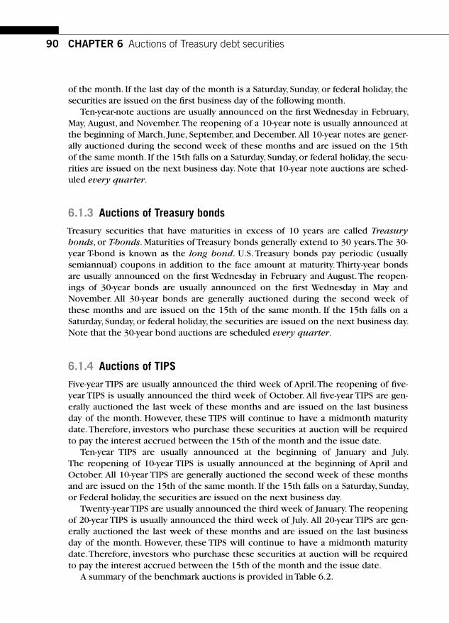
90 CHAPTER 6 Auctions of Treasury debt securities
of the month. If the last day of the month is a Saturday, Sunday, or federal holiday, the securities are issued on the fi rst business day of the following month.
Ten-year-note auctions are usually announced on the fi rst Wednesday in February, May, August, and November. The reopening of a 10-year note is usually announced at the beginning of March, June, September, and December. All 10-year notes are gener-ally auctioned during the second week of these months and are issued on the 15th of the same month. If the 15th falls on a Saturday, Sunday, or federal holiday, the secu-rities are issued on the next business day. Note that 10-year note auctions are sched-uled every quarter.
6.1.3 Auctions of Treasury bonds
Treasury securities that have maturities in excess of 10 years are called Treasury bonds, or T-bonds. Maturities of Treasury bonds generally extend to 30 years. The 30-year T-bond is known as the long bond. U.S. Treasury bonds pay periodic (usually semiannual) coupons in addition to the face amount at maturity. Thirty-year bonds are usually announced on the fi rst Wednesday in February and August. The reopen-ings of 30-year bonds are usually announced on the fi rst Wednesday in May and November. All 30-year bonds are generally auctioned during the second week of these months and are issued on the 15th of the same month. If the 15th falls on a Saturday, Sunday, or federal holiday, the securities are issued on the next business day. Note that the 30-year bond auctions are scheduled every quarter.
6.1.4 Auctions of TIPS
Five-year TIPS are usually announced the third week of April. The reopening of fi ve-year TIPS is usually announced the third week of October. All fi ve-year TIPS are gen-erally auctioned the last week of these months and are issued on the last business day of the month. However, these TIPS will continue to have a midmonth maturity date. Therefore, investors who purchase these securities at auction will be required to pay the interest accrued between the 15th of the month and the issue date.
Ten-year TIPS are usually announced at the beginning of January and July. The reopening of 10-year TIPS is usually announced at the beginning of April and October. All 10-year TIPS are generally auctioned the second week of these months and are issued on the 15th of the same month. If the 15th falls on a Saturday, Sunday, or Federal holiday, the securities are issued on the next business day.
Twenty-year TIPS are usually announced the third week of January. The reopening of 20-year TIPS is usually announced the third week of July. All 20-year TIPS are gen-erally auctioned the last week of these months and are issued on the last business day of the month. However, these TIPS will continue to have a midmonth maturity date. Therefore, investors who purchase these securities at auction will be required to pay the interest accrued between the 15th of the month and the issue date.
A summary of the benchmark auctions is provided in Table 6.2 .
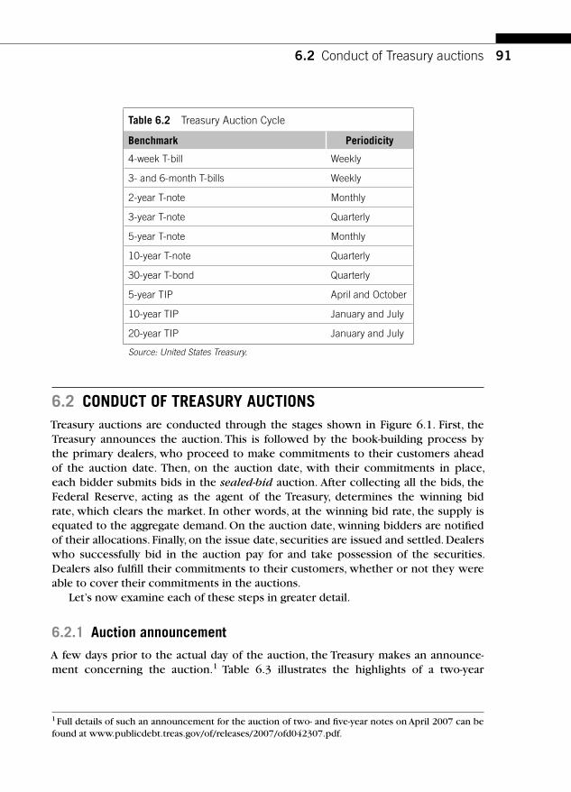
91
6.2 CONDUCT OF TREASURY AUCTIONS Treasury auctions are conducted through the stages shown in Figure 6.1 . First, the Treasury announces the auction. This is followed by the book-building process by the primary dealers, who proceed to make commitments to their customers ahead of the auction date. Then, on the auction date, with their commitments in place, each bidder submits bids in the sealed-bid auction. After collecting all the bids, the Federal Reserve, acting as the agent of the Treasury, determines the winning bid rate, which clears the market. In other words, at the winning bid rate, the supply is equated to the aggregate demand. On the auction date, winning bidders are notifi ed of their allocations. Finally, on the issue date, securities are issued and settled. Dealers who successfully bid in the auction pay for and take possession of the securities. Dealers also fulfi ll their commitments to their customers, whether or not they were able to cover their commitments in the auctions.
Let’s now examine each of these steps in greater detail.
6.2.1 Auction announcement
A few days prior to the actual day of the auction, the Treasury makes an announce-ment concerning the auction. 1 Table 6.3 illustrates the highlights of a two-year
6.2 Conduct of Treasury auctions
1 Full details of such an announcement for the auction of two- and fi ve-year notes on April 2007 can be found at www.publicdebt.treas.gov/of/releases/2007/ofd042307.pdf.
Table 6.2 Treasury Auction Cycle
Benchmark Periodicity
4-week T-bill Weekly
3- and 6-month T-bills Weekly
2-year T-note Monthly
3-year T-note Quarterly
5-year T-note Monthly
10-year T-note Quarterly
30-year T-bond Quarterly
5-year TIP April and October
10-year TIP January and July
20-year TIP January and July
Source: United States Treasury.

92 CHAPTER 6 Auctions of Treasury debt securities
Auctionannouncement
Book building in thewhen-issued market
Bidding insealed-bid auctions
Auction results areannounced
Securities issued andsettled on issue date
FIGURE 6.1
Steps in Treasury Auctions
Table 6.3 Two-Year T-Note Auction Announcement
Announcement date April 23, 2007
Offering amount $18 billion
Term Two-year T-note
Auction date April 25, 2007
Issue date April 30, 2007
Maturity date April 30, 2009
Dated date April 30, 2007
Coupon To be set at the auction based on the highest accepted competitive bid
Coupon payment dates October 31 and April 30
Source: United States Treasury.

93
Treasury note auction announcement for April 2007. Note that the coupon will be set in the auction on the basis of the highest winning yield in the auction and hence will not be known at the time of announcement. The dated date refers to the fi rst date from which coupons begin to accrue. All Treasury auctions are sealed-bid, uniform price auctions in which all the winning bidders pay exactly the same price.
Note that the announcement occurred two days prior to the day of the auc-tion. During this two-day period, bidders will engage in the book-building process, which enables them to assess the demand and formulate their bidding strategies on auction day.
6.2.2 When-issued trading and book building
Forward trading among potential bidders in the auction precedes U.S. Treasury auctions. This practice also exists in the Japanese government bond auc-tions. This forward market, known as the when-issued (WI) market, is an integral part of the Treasury bidding and distribution system currently in place. In when-issued trading, the bidders are liable to enter the auction and bid with prior short or long positions. Consequently, this affects their bidding strategies and the outcome of the auction.
During the period between the auction announcement date and the issue date (which varies from two to fi ve days), when-issued trading occurs. This practice was offi cially sanctioned in August 1981 and was initiated to encourage trading in Treasury securities after the announcement of the auction but before the securities are actually issued. Prior to the Treasury’s scheduled auction date for a given secu-rity, dealers and investors actively participate in the when-issued market. In this market, dealers and investors may either take long positions or short positions in the security (to be auctioned by the Treasury) for a future settlement on the issue date. Thus WI trades are forward contracts with a settlement date equal to the issue date. The trading in this market is done in terms of the yields at which the securities are expected to be sold. The Treasury announces the coupon of the issue after all the bids are received. After the coupon is announced, the issue trades on a price basis one day after the auction. Typically the securities are issued about one to fi ve days following the auction date.
6.2.3 Auction mechanisms
All auctions in the Treasury markets are sealed-bid auctions in the sense that other bidders do not know bids made by any individual bidder. Two types of auction mechanisms are used in the markets: discriminatory auctions and uniform price auctions. Under each mechanism, two types of bids are invited. One is known as a noncompetitive bid, in which bidders can specify the amount that they would like to buy but do not specify the price. The Treasury always fi lls
6.2 Conduct of Treasury auctions

94 CHAPTER 6 Auctions of Treasury debt securities
noncompetitive bids, but the bids may not exceed $5 million per bidder. The other type of bid, known as a competitive bid, is the more important part of the auction. Here bidders specify the quantity that they would like to buy and the price at which they would like to buy. Each dealer can submit multiple price-quantity bids; in other words, dealers can submit their demand curves. After receiving all the bids, Treasury will aggregate and determine the aggregate demand for its securities in the auction. From the total supply available, the total demand in the noncompetitive bids will be subtracted to determine the net supply that is available to the competitive bidders.
6.2.4 Uniform price auctions
Since 1999, all U.S. Treasury auctions have been uniform price auctions. The dis-criminatory procedure has been discontinued. Nonetheless, we discuss both types of auctions here since both are widely used throughout the global government debt markets.
The total quantity bid by the investors in the noncompetitive tender is subtracted from the aggregate amount of the security that the Treasury has to offer in the auction to determine the amount that will be sold via competitive bids. The U.S. Treasury will choose the yield at which the aggregate demand exhausts the supply to the competitive tender. This market-clearing yield is known as the stop-out yield. (This means that the Treasury starts at the lowest yield and works its way down to the higher yield. At the highest winning yield, the stop-out yield, the allocation will be done on a pro rata basis.) It is worth emphasizing that each successful competitive bidder pays the stop-out yield. The bidders in the noncompetitive tender also pay the stop-out yield. The bidders on the noncom-petitive tender are assured of the quantities that they bid for at the stop-out yield established in the competitive tender. So, noncompetitive bidders face no quantity uncertainty. Since the Treasury restricts the bids in the noncompetitive sector to $5 million par amount of the auctioned security, only small investors and institutions tend to participate in this sector of the auctions. There is a limit on the maximum number of securities awarded to a single bidder. Under the 35% rule, the bidder’s net long position in the auction at any one yield inclusive of futures, forwards, and when-issued markets may not exceed 35% of the amount of the security in the auc-tion. When the issue is reopened, the net long position will include any position in the outstanding security as well. Once the bidding is completed, the 35% rule is lifted.
To recap, in uniform price auctions, the bids are ordered from the most aggressive to the least aggressive. Priority will be given in the allocation of supply to the most aggressive bids, followed by the next most aggressive bids, and so on. The Treasury will determine the bid at which the supply will be exhausted and will use that bid uniformly to allocate securities to all bidders, irrespective of their actual bids. In this sense, there is no discrimination.

95
Example 6.1 A hypothetical uniform price auction example is presented in Figure 6.2 to highlight the issues. In this example, the seller wants to auction $16 billion of Treasury securities.
6.2 Conduct of Treasury auctions
Size: $16 billion
Competitivetender
(Available: $15 billion)
Noncompetitivetender
Demand: $1 billion
Bids submitted in non-competitive tender must specifyonly quantity demanded and must be below $5 million.
FIGURE 6.2
Hypothetical Example of a Uniform Price Auction
The total demand in the noncompetitive tender was $1 billion. This must be met under all conditions. Therefore, the supply that is available to the competitive tender is $15 billion.
Assume that Dealer A submits the demand function shown in Figure 6.3 . His most aggressive bid is at 5.72% for $500 million par and his least aggressive bid is at 5.75% for $600 million par. The demand curve submitted by Dealer B is also shown. The Treasury will aggregate the demand curves submitted by all dealers and sort them from the most aggressive to the least aggressive bid. Figure 6.3 shows the total demand curve with the most aggressive bid at 5.70% (by dealers other than A or B) for $5 billion par. The Treasury will march down the total demand curve until the aggregate demand equals the supply. Note that this happens at a yield of 5.73%. Then at this yield, known as the stop-out yield , all bidders who bid at or lower than 5.73% will be awarded the securities. Note that every bidder pays the same price. At 5.73%, the demand is $5 billion, but the remaining supply is only $2.5 billion, because the more aggressive bidders would have been awarded $12.5 billion of the supply.
Therefore, at the stop-out yield, the supply is prorated to the dealers who bid at that yield; only 50% of the demand would be met at the stop-out yield in our example.
How does the Treasury set the coupon? The coupon is simply the stop-out yield rounded down to the nearest eighth. In the context of our example, the coupon would be set at 5.625%. This would imply that the new security would sell at a slight discount, since the coupon is a shade below the market-clearing yield. This is typi-cally the case in all Treasury auctions.

96 CHAPTER 6 Auctions of Treasury debt securities
Note that the fact that every bidder will pay the same price, irrespective of what they bid, encourages the bidders to bid more aggressively. This helps the seller because the effect of more aggressive bidding, ex-ante, will lower the stop-out yield, ex-post.
Moving from our hypothetical example to a real-life example, the auction awards of the uniform price sealed-bid auction announced in Table 6.3 are presented in Table 6.4 for the April 2007 two-year notes. 2
The ratio of the bids received to the amount awarded is computed and is used as a metric of how well the auction went; the higher this ratio, the stronger the auction is, ceteris paribus. This ratio is called the bid-cover ratio. For the April 2007 two-year T-note auction, the bid-cover ratio was 2.93. 3
Note that the stop-out yield was 4.606%. Bidders who bid at yields above the stop-out yield did not win any security in the auction. All the other bidders (who bid more aggressively in the auction) received the security at a common market-clearing (stop-out) yield of 4.606%. Remember that even the most aggressive bidder paid only 4.606%. This has important implications for both the level of bidding in these auc-tions and for the possible dispersion of the bids.
2 More details about the results of this auction can be found at www.publicdebt.treas.gov/of/releases/2007/ofk0425071.pdf.3 Bid-cover ratio � �52 768 18 000 2 93. / . . .
Uniform price auctions
Competitivetender
(Available: $15 billiion)
Dealer A Dealer BTotal DemandA�B�....
Quantity Quantity QuantityYield Yield Yield
600
500
400
500
500
400
600
5.72%
5.73%
5.74%
5.75%
1000 5.71%
5.72%
5.73%
5.74%
5000
5000
2500
5000
5.70%
5.71%
5.72%
5.73%
Stop out yield is 5.73%
FIGURE 6.3
Hypothetical Example of Demand Schedules in a Uniform Price Auction

97
6.2.5 Discriminatory auctions
In discriminatory auctions as well, typically the governments invite two types of bid: competitive and noncompetitive. In competitive bids, primary dealers submit both prices and quantities. Each competitive bidder is allowed to submit multiple bids. There is typically a ceiling on how much can be submitted in a noncompetitive ten-der. The government acts as a perfectly discriminating monopolist by awarding the security to the highest bidder and working its way down until the entire amount is sold. (This implies that the government starts at the lowest yield and works its way to the highest yield. At the highest winning yield, all allocation is done on a pro rata basis.) The bidders in noncompetitive tender get the amount that they bid at a yield equal to the weighted average of the winning yields in the competitive tender.
In discriminatory auctions, the most aggressive bids will be fi lled fi rst at the price at which they were bid. The remaining net supply will be used to fi ll the next aggres-sive bid at the price at which it was bid, until the supply is exhausted. Because bid-ders actually end up paying the prices that they bid, there is discrimination: The most aggressive bidder will pay more than the next aggressive bidder, and so on.
Let’s reconsider the previous hypothetical example under the assumption that the dealers knew that it was going to be done as a discriminatory auction. How would their bidding strategy change? Bidders will realize that if they are too aggres-sive, they will increase the likelihood of winning the bids but will end up paying their aggressive price. This will tend to promote two things: First, the bidders will have an incentive not to bid too aggressively. Second, they will want to know the consensus value of the security so that they can “shade down ” their bids to this con-sensus value. We present a possible bidding scenario in Figure 6.4 .
The Treasury marches down the aggregate demand curve, allocating securities until demand equals supply. The allocation is done at the yield levels that were bid. In this respect, discriminatory auctions differ from uniform price auctions: The most aggressive bidder wins buts ends up paying a very high price. This leads to the
6.2 Conduct of Treasury auctions
Table 6.4 Auction Results for a Two-Year T-Note
Tender Type Tendered Accepted
Competitive $52.066 billion $17.298 billion
Noncompetitive $0.702 billion $0.702 billion
Total $52.768 billion $18.000 billion
Federal Reserve $4.777 billion $4.777 billion
Median yield: 4.590% Coupon: 4.50%
Highest winning yield: 4.606% Price: 99.799666
Source: United States Treasury.

98 CHAPTER 6 Auctions of Treasury debt securities
concept of “winner’s curse, ” which we discuss later. In this example, Treasury would have sold $5 billion at 5.75%, another $5 billion at 5.76%, and $2.50 billion at 5.77%. At a yield of 5.78%, the aggregate demand is $5 billion, but the remaining supply is only $2.5 billion. Bidders at this yield level will receive a pro rata allocation: They will get exactly 50% of their demand. The Treasury will receive a weighted average yield of 5.7417% in this auction, calculated as follows: The Treasury will round down to the nearest eighth and set the coupon at 5.75%.
The U.S. Treasury no longer uses discriminatory auctions for selling its debt, but many other countries do. Table 6.5 illustrates the allocation in a discriminatory auc-tion that was conducted by the Bank of Japan for a Japanese government bond (JGB) auction.
In this fi ve-year JGB auction, only 6.76% of the bids were allotted at the lowest accepted price, and only a small fraction (176 billion yen) was accepted at the non-competitive bids.
Discriminatory auctions
Competitivetender
(Available: $15 billion)
Dealer A Dealer BTotal DemandA�B�....
Quantity Quantity QuantityYield Yield Yield
600
500
400
500
500
400
600
5.76%
5.77%
5.78%
5.79%
1000 5.75%
5.76%
5.77%
5.78%
5000
5000
2500
5000
5.75%
5.76%
5.77%
5.78%
FIGURE 6.4
Hypothetical Example of a Discriminatory Price Auction
Table 6.5 Five-Year JGB Security Auction
Amounts of CompetitiveBids (Billion Yen)
Amounts of Accepted
Bids (Billion Yen)
Lowest AcceptedPrice (Per 100 Yen)
Yield at the Lowest Accepted
Price
Weighted Average Price (Per 100 Yen)
6,855.50 1,716.20 100.18 1.261% 100.21
Note: Five-year security; auction date: July 8, 2008; issue date: July 11, 2008; maturity date: June 20, 2013; nominal coupon: 1.3%. Source: Ministry of Finance, Government of Japan.

99
6.3 AUCTION THEORY AND EMPIRICAL EVIDENCE Empirical evidence indicates that the uniform price auction appears to have a higherbid-cover ratio and a higher dispersion of winning bids. Traders familiar with the bidding process confi rm that this is fairly typical in their experience. At fi rst glance, it might appear that the Treasury is losing out in uniform price auctions: Bidders who bid more aggressively only end up paying the common winning (highest) stop-out yield. The reason for their aggressive bidding is precisely that the bids are not dis-criminated. Indeed, if lots of bidders bid aggressively, the stop-out yield will go down, refl ecting the overall aggressiveness. This will increase the revenue of the Treasury and lower the cost of public debt.
In both auction mechanisms, bidders face quantity uncertainty. In the uniform price auction presented, bidders who bid most aggressively were allotted the secu-rity fi rst, and as the supply was depleted, the bidders who exactly bid at the stop-out yield ended up receiving less than their total demand. The U.S. Treasury makes a pro rata allocation for bidders at the stop-out yield. Bidders in discriminatory auc-tions are subject to similar quantity uncertainty. This is a signifi cant quantity risk that should also encourage more aggressive bidding. In addition, bidders may also diver-sify their bids by submitting multiple price-quantity bids.
6.3.1 Winner’s curse and bid shading
Winner’s curse refers to the possibility that the aggressive bidder in a discriminatory auction will end up paying too much relative to the market consensus. Anticipating this possibility, bidders tend to shade down their bids relative to the true value of the security, to minimize the winner’s curse, and they invest considerable resources in pre-auction information gathering to learn more about the market consensus so that their bids are not out of line with the market consensus. The Treasury loses money because of the winner’s curse but is able to exercise the power of a discriminating monopolist by selling the same security through marching down the demand curve submitted by the bidders.
In the uniform price auction, the Treasury allocates the security at a common price; hence, it gives up the power to discriminate. On the other hand, bidders can be more aggressive since they pay the same price irrespective of their bids. The incentive to gather pre-auction information is possibly less in this auction. Therefore, the winner’s curse should be less an issue in uniform price auctions.
Table 6.6 summarizes the available evidence on the winner’s curse. Note that the markup on Treasury bills has varied from four basis points to one basis point. For coupon issues, Simon (1994) estimates a markup of less than a basis point. As shown in Table 6.6, researchers have employed several different methods to assess the suc-cess of a particular auction format in achieving a high selling price. To measure bid shading, we must subtract from the “true value ” of the security, the actual price paid by the dealers to Treasury. Such a difference will provide an estimate of the loss to the Treasury.
6.3 Auction theory and empirical evidence

100 CHAPTER 6 Auctions of Treasury debt securities
The markups have varied from 3/8 to 4 basis points. To the extent that markups are lower in uniform price auctions, that would be evidence in favor of using uni-form price auction format. Nyborg and Sundaresan (1996) suggest that this might be the case on the basis of their analysis of discriminatory and uniform price auc-tions of fi ve- and two-year T-notes in the United States. The U.S. Department of Treasury conducted its own studies in 1995 and 1998. Their results also showed that the two- and fi ve-year notes sold by the uniform price auction procedure since September 1992 tend to have lower markups compared to others sold by mul-tiple-price (discriminatory) auction procedures. In addition, they found that the uniform price auctions generated broader participation and award distribution.
6.4 AUCTION CYCLES AND FINANCING RATES Practitioners have noted that repo rates for the most recently issued notes become increasingly special until the next issue is announced. This cyclical pattern appears to be pervasive for all benchmark maturities. Keane (1996) conducted an analysis of this question and concluded the following: “Our analysis of the data reveals a strong positive correlation between repo specialness and the Treasury auction cycle. On average, repo rates for the most recently issued notes become increasingly special until the next issue is announced. ”Figure 6.5 shows that this effect is signifi cant.
This evidence suggests that newly issued (on-the-run) Treasury debt trades special in the fi nancing markets. This evidence can also be viewed in the context of the evi-dence presented in Figure 5.8 in Chapter 5, where we found patterns in the spread between GC repo and special fi nancing rates over the 1987 –1992 period.
Table 6.6 Markups/Bid Shading: Empirical Evidence
Source Data and Sample Measure of Markup Estimated Markups
Cammack (1991) T-bills (1973 –1984) Auction average yield minus average of WI at close on auction date
4 basis points
Spindt and Stoltz (1992)
T-bills (1982 –1988) Auction average yield minus bid of WI 30 minutes before auction
1.5 basis points
Bikhchandani et al. (1994)
T-bills (1986 –1988) Auction average yield minus bid of WI at 1:00 p.m.
1 basis point
Simon (1994) Coupon debt (1990–1991)
Auction average yield minus bid of WI at 1:00 p.m.
3 8/ basis point

101
As a consequence, rational buyers will know that they could lend the security in the repo market and borrow money at the attractive (special) repo rates. Hence they should be willing to pay a premium for it. This suggests that on-the-run issues are more expensive than off-the-run issues. Sundaresan (1994) , Duffi e (1996) , and Krishnamurthy (2002) have explored related questions in more detail.
SUGGESTED READINGS AND REFERENCES Bikchandani , S., & Huang , C. ( 1993 ) . The economics of treasury securities markets . Journal of
Economic Perspectives , 7 , 117 – 134 .
Cammack , E. ( 1991 ) . Evidence of bidding strategies and the information in treasury bill auctions . Journal of Political Economy , 99 , 100 – 130 .
Duffi e , D. ( 1996, June ) . Special repo rates . Journal of Finance , 51 , 493 – 526 .
Keane , F. ( 1996, September ) .Repo rate patterns for new treasury notes . Current Issues in Economics and Finance , 2 ( 10) .
Suggested readings and references
120
100
80
60
40
20
22 20 18 16 14 12 10 8 6 4 2 00
Bas
is p
oint
s
Five-year note
Two-year note
Business days to next issuance
Notes: The spread is calculated using overnight rates from June 12,1992, toJanuary 25, 1995. The monthly auction cycle extends from one issue date to thenext. The shaded area marks announcement days for the next issue.
Average spread between general and special reporates for two-and five-year treasury notesMonthly Auction Cycle
FIGURE 6.5
Effect of Auction Cycles on Repo Rates Source: Frank Keane, “ Repo Rate Patterns for New Treasury Notes, ” Current Issues in Economics and Finance , September 1996, Vol. 2, No. 10.

102 CHAPTER 6 Auctions of Treasury debt securities
Krishnamurthy , A. ( 2002) . The bond/old-bond spread . Journal of Financial Economics , 66 ( 2) , 463 – 506 .
Friedman , M. ( 1991, 28 August ) . How to sell government securities . Wall Street Journal .
Nyborg, K. , & Sundaresan , S. ( 1996) . Discriminatory versus uniform treasury auctions: Evidence from when-issued transactions . Journal of Financial Economics , 42 , 63 – 104 .
Simon , D. P. ( 1994) . Markups, quantity risk and bidding strategies at treasury coupon auctions . Journal of Financial Economics , 35 , 43 – 62 .
Sundaresan , S. ( 1994, September ) . An empirical analysis of U.S. treasury auctions: implications for auction and term structure theories . The Journal of Fixed Income, 4(2), 35–50 .
Vickrey , W. ( 1961) . Counterspeculation, auctions, and competitive sealed tenders . Journal of Finance , 16 , 8 – 37 .

Analytics of fi xed income markets 2
PART

This page intentionally left blank

105
CHAPTER
CHAPTER SUMMARY We develop the concept of dollar value of an 01 (DV01) or price value of a basis point (PVBP) to measure risk of fi xed-income securities. The concept of price elas-ticity of debt securities with respect to interest rates is developed, and various dura-tion measures such as Macaulay duration and modifi ed duration are described. The chapter develops the concept of convexity and describes its measurement. Through several examples, this chapter develops these concepts and applies them to trading and hedging applications such as yield curve trades (steepening or fl at-tening) and butterfl y strategies. Alternative measures of duration such as effective duration are described to compute the risk of securities for which cash fl ows are sensitive to interest rates.
Fixed income securities display varying price sensitivities to changing interest rates. The purpose of this chapter is to develop certain quantitative measures of interest rate risk. These measures will enable us to compare the interest rate risks of various securities and implement risk management strategies.
7.1 DV01/PVBP OR PRICE RISK The risk of a bond is the change in its price due to changes in the interest rates in the market. DV01 or PVBP measures the price change in debt securities for a basis point (or 0.01%) change in interest rates. If P is the price of the bond and y is its yield, a measure of the bond’s risk is the change in its price for a change in its yield. This is denoted by the fi rst derivative of the bond price with respect to its yield, or dP/dy. Let’s try to get some intuition behind this concept by looking at an example.
Bond mathematics: DV01, duration, and convexity 7
Fixed Income Markets and Their DerivativesCopyright 2009 by Academic Press. Inc. All rights of reproduction in any form reserved.

106 CHAPTER 7 Bond mathematics: DV01, duration, and convexity
Consider a bond with one year to maturity. It pays a 4% coupon semiannually on a par value of $100 and has a YTM of 6%. The price of the bond is
P �
�
�
�
�4
10 06
2
104
10 06
2
101 913472. .
. .⎛⎝⎜⎜⎜
⎞⎠⎟⎟⎟
⎛⎝⎜⎜⎜
⎞⎠⎟⎟⎟
We want to know what will happen to its price if the yields change by a small amount, say, one basis point, to 6.01%. The new price will be
′⎛⎝⎜⎜⎜
⎞⎠⎟⎟⎟
⎛⎝⎜⎜⎜
⎞⎠⎟⎟⎟
P �
�
�
�
�4
10 0601
2
104
10 0601
2
101 9037642. .
. ..
We can approximate the risk dP/dy by measuring the price difference P P� �′ 0 009705. . Often debt securities are traded in units of $1 million par amounts. Hence we can express the DV01 of a $1 million par amount of this security as follows:
P P� � � � �′ ( . . ) , . .101 91347 101 903764 10 000 97 053
Note that we compute the price change taking into account the fact that prices are quoted in percentages —namely, P P� �′ (101.91347 � 101.903764) �
1,000,000/100 � 97.053. Roughly we are estimating the slope of the tangent to the price-yield relationship at 6% yield. This is represented in Figure 7.1 .
We can get a slightly better estimate of the tangent by moving the yield down by 0.5 basis point ( y � 5.995%) and up by 0.5 basis point ( y � 6.005%) around 6% as follows.
P �
�
�
�
�4
10 05995
2
104
10 05995
2
2. .⎛⎝⎜⎜⎜
⎞⎠⎟⎟⎟
⎛⎝⎜⎜⎜
⎞⎠⎟⎟⎟
101.91832..
′⎛⎝⎜⎜⎜
⎞⎠⎟⎟⎟
⎛⎝⎜⎜⎜
⎞⎠⎟⎟⎟
P �
�
�
�
�4
10 06005
2
104
10 06005
2
2. .101.908622.
The estimated price risk per $1 million par may be computed as before and is given by
dP dy/ � 97.05992.
The difference between the fi rst estimate and the second estimate tends to be small but can be relatively more important for debt securities with long maturity.

107
Using the � PRICE function of Excel it is fairly easy to compute PVBP or DV01 of debt securities as shown in the following example.
Example 7.1 For all the benchmark Treasury securities shown in Table 7.1 , compute the DV01 (PVBP) for $1 million par value. Explain the differences that you found. Show all relevant calculations. Assume a settlement date of September 12, 2007.
7.1 DV01/PVBP or price risk
PVBP
Price-yield curve
6%
Yield to maturity
Pric
e
101.91347
FIGURE 7.1
Price-Yield Curve and PVBP
Table 7.1 Benchmark Treasury Quotes
Maturity Date Coupon Yield to Maturity Benchmark Maturity
8/31/2009 4.00% 3.933% 2 years
5/15/2010 4.50% 3.945% 3 years
8/31/2012 4.125% 4.056% 5 years
8/15/2017 4.75% 4.364% 10 years
5/15/2037 5.00% 4.646% 30 years
Source: Bloomberg.
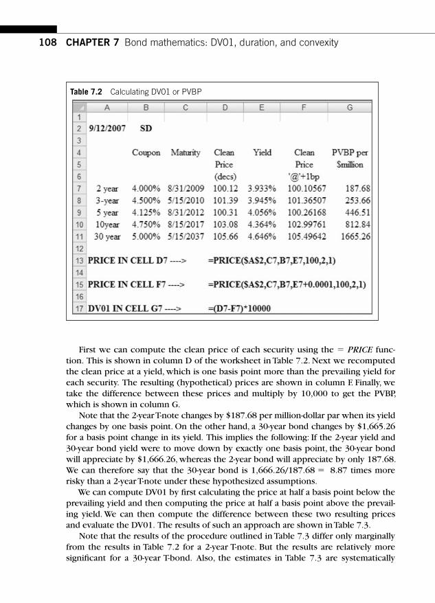
108 CHAPTER 7 Bond mathematics: DV01, duration, and convexity
First we can compute the clean price of each security using the � PRICE func-tion. This is shown in column D of the worksheet in Table 7.2 . Next we recomputed the clean price at a yield, which is one basis point more than the prevailing yield for each security. The resulting (hypothetical) prices are shown in column F. Finally, we take the difference between these prices and multiply by 10,000 to get the PVBP, which is shown in column G.
Note that the 2-year T-note changes by $187.68 per million-dollar par when its yield changes by one basis point. On the other hand, a 30-year bond changes by $1,665.26 for a basis point change in its yield. This implies the following: If the 2-year yield and 30-year bond yield were to move down by exactly one basis point, the 30-year bond will appreciate by $1,666.26, whereas the 2-year bond will appreciate by only 187.68. We can therefore say that the 30-year bond is 1,666.26/187.68 � 8.87 times more risky than a 2-year T-note under these hypothesized assumptions.
We can compute DV01 by fi rst calculating the price at half a basis point below the prevailing yield and then computing the price at half a basis point above the prevail-ing yield. We can then compute the difference between these two resulting prices and evaluate the DV01. The results of such an approach are shown in Table 7.3 .
Note that the results of the procedure outlined in Table 7.3 differ only marginally from the results in Table 7.2 for a 2-year T-note. But the results are relatively more signifi cant for a 30-year T-bond. Also, the estimates in Table 7.3 are systematically
Table 7.2 Calculating DV01 or PVBP
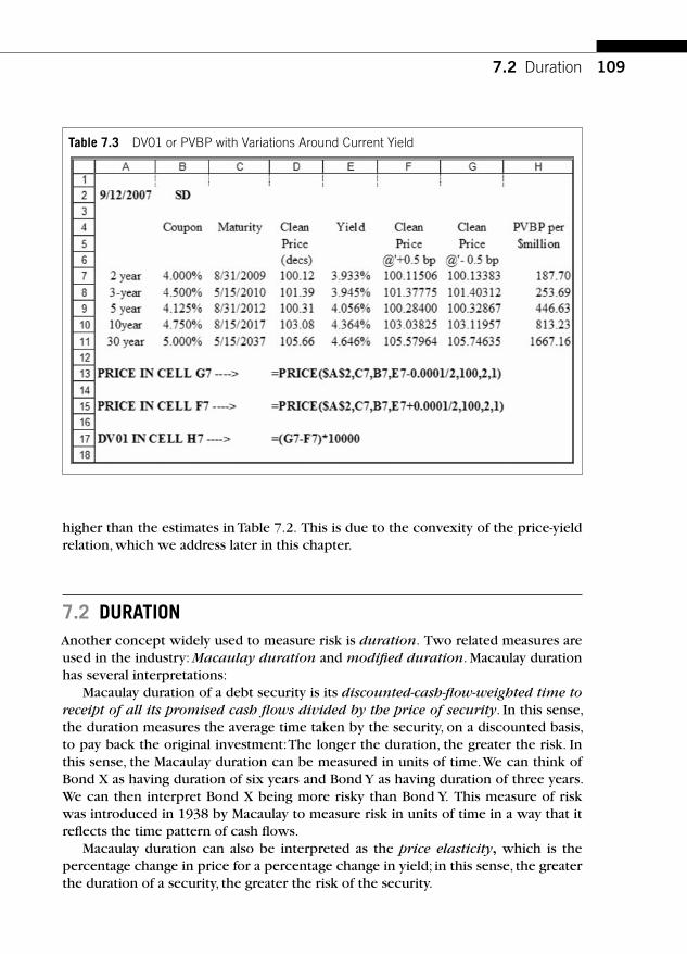
109
higher than the estimates in Table 7.2 . This is due to the convexity of the price-yield relation, which we address later in this chapter.
7.2 DURATION Another concept widely used to measure risk is duration. Two related measures are used in the industry: Macaulay duration and modifi ed duration. Macaulay duration has several interpretations:
Macaulay duration of a debt security is its discounted-cash-fl ow-weighted time to receipt of all its promised cash fl ows divided by the price of security. In this sense, the duration measures the average time taken by the security, on a discounted basis, to pay back the original investment: The longer the duration, the greater the risk. In this sense, the Macaulay duration can be measured in units of time. We can think of Bond X as having duration of six years and Bond Y as having duration of three years. We can then interpret Bond X being more risky than Bond Y. This measure of risk was introduced in 1938 by Macaulay to measure risk in units of time in a way that it refl ects the time pattern of cash fl ows.
Macaulay duration can also be interpreted as the price elasticity , which is the percentage change in price for a percentage change in yield; in this sense, the greater the duration of a security, the greater the risk of the security.
7.2 Duration
Table 7.3 DV01 or PVBP with Variations Around Current Yield

110 CHAPTER 7 Bond mathematics: DV01, duration, and convexity
We consider all these interpretations in detail in the context of the following example.
Interpretation 7.1 Macaulay duration is the discounted-cash-fl ow-weighted time to receive all its promised cash fl ows divided by the price of the security.
Consider also a three-year bond paying a coupon of 5% per annum, also yielding 5% yield to maturity. For simplicity we assume annual coupons.
The price of the three-year zero is 100 1 05 86 38383/ . .� . The discount factors for the fi rst three years are: 1 05 0 952381 1 051 2. . , .� �� �
0 907029. , and 1 05 0 8638383. .� � . As shown in Table 7.4 , we fi nd that the sum of discounted-cash-fl ow-weighted promised cash fl ows scaled by the price gives us Macaulay duration.
Mathematically, we compute the duration as follows:
D �� � � � � � � �
�1 5 0 952381 2 5 0 907029 3 105 0 863838
1002 859
. . .. .
If we set the coupon equal to zero in the previous example (and noting that the price of a three-year zero paying 100 after three years is the discounted value of 100), we fi nd that the equation reduces to the following:
D �� �
�3 100 0 863838
1001 05
3 003
.
.
. .
This gives us the result that the Macaulay duration of a zero coupon bond is simply its time left to maturity.
Table 7.4 Duration as Cash-Flow-Weighted Time to Cash Flows Divided by Price
Year Discount Factors Cash Flows Cash-Flow-Weighted Time
Discounted-Cash-Flow-Weighted Time
1 0.952381 5 5 4.762
2 0.907029 5 10 9.070
3 0.863838 105 315 272.109
Total � 285.941
Price � 100
Sum of discounted-cash-fl ow-weighted times divided by price → 2.859

111
Returning to coupon bonds, we can defi ne Macaulay duration in more general terms as follows:
D
iC
y
P
ii
i
N
��� ( )
.11
∑
(7.1)
In the general defi nition of Macaulay duration, in Equation 7.1, N is the number of years until maturity, y is the yield to maturity, and the cash fl ow at period i is denoted by Ci .
One of the applications of this concept is in bond portfolio immunization: If we can fund liabilities with assets in such a way that their Macaulay durations are the same, such a portfolio is immune from interest rate fl uctuations. This is because the price elasticity of assets is the same as the price elasticity of liabilities. Hence their fl uctuations cancel each other out.
Interpretation 7.2 Duration is the price elasticity of interest rates; duration is also the price elasticity, which is the percentage change in price for a percentage change in yield.
Formally, the elasticity measure of duration is referred to as the Macaulay duration and is represented as follows:
D � �the percentage change in price of a bond
the percentage cchange in the yield of the bond
� �� �
� � �dP P
d y y
dP P
dy1 11
( ) ( )( yy).
This leads to the expression for Macaulay duration, as shown here:
DdP P
dyy� � �( ).1 (7.2)
The negative sign is just a reminder that prices and yields move in opposite direc-tions. We take the percentage change in price of a bond, denoted by dP P , and then divide that quantity by the percentage change in the yield of the bond, denoted
by dy
y1 �.
We can rewrite the Equation 7.2 as follows:
DdP
dy Py� � �
11( ).
With semiannual compounding, sometimes the following convention is also used:
DdP
dy Py� � �
11 2( / ).
7.2 Duration

112 CHAPTER 7 Bond mathematics: DV01, duration, and convexity
We note that � dP dy/ is just the DV01 of the bond. Using this information in Equation 7.2, we conclude the following:
DDV
Py� �
011( ). (7.3)
In Table 7.5 we carry out these calculations for the three-year bond and fi nd that the price elasticity defi nition of duration also leads us to the same answer: D � 2.86.
In this way of thinking about risk, we say that duration measures the elasticity of the bond price to interest rates: the percentage change in bond price for a percent-age change in interest rates. Note that we are not measuring the change in interest rates but the percentage change in interest rates.
Another related measure is modifi ed duration (MD). Modifi ed duration is the per-centage change in price for a change in yield. Modifi ed duration is denoted as
MDdP P
dy� − . (7.4)
Using the defi nition of DV01 and rearranging Equation 7.4, we get the modifi ed duration as follows:
MDDV
P�
01. (7.5)
Note that the price, P, in Equation 7.5 is the dirty price. From Table 7.5 we can compute the DV01 as follows: Price at a yield of 4.995% is 100.0136175 (rounded
Table 7.5 Duration as Price Elasticity of Interest Rates

113
to seven decimals in Table 7.5 ). Price at a yield of 5.005% is 99.986385 (rounded to seven decimals in Table 7.5 ).
DV 01 100 0138175 99 986385 10 000 272 3248049� � � �( . . ) , . .
Using this equation, we compute the Macaulay duration as:
D � � �272 3248049
1001 05 2 86
.. . .
Modifi ed duration is simply DV01 divided by the price, which leads to MD � 2.72. What is the economic intuition behind modifi ed duration? Let’s rearrange
Equation 7.4 to get:
dP
PMD dy� � � . (7.6)
This says that the percentage change in the bond price is the modifi ed dura-tion multiplied by the change in its yield: In other words, the higher the modifi ed duration of a bond, the higher is its percentage change to a change in its yield. We can slightly rewrite Equation 7.6 to obtain an expression for the change in the bond price as follows:
dP MD P dy� � � � . (7.7)
Consider a bond selling at par, with MD � 7. Equation 7.7 says that a 1% increase in a bond’s yield will produce a decrease in price of 7%.
7.2.1 Excel applications
Excel has functions for calculating duration measures. They are shown in the Excel spreadsheet in Table 7.6 .
Modifi ed duration is always smaller than Macaulay duration and is more exten-sively used in practice.
Table 7.7 provides the duration of benchmark debt securities issued by the Treasury.
Note that duration is increasing with maturity but not in direct proportion:A 30-year bond has a duration of only 15.90 years, whereas the 10-year note has a duration of 8.03 years.
In fact, we can show that even bonds with infi nite life (perpetuity) will have only a fi nite duration. To see this, let’s consider the price of a perpetuity given in Equation 2.10 in Chapter 2:
Pc
y=
100.
7.2 Duration

114 CHAPTER 7 Bond mathematics: DV01, duration, and convexity
Table 7.6 Excel Functions for Duration
Table 7.7 Duration Estimates for Treasury Benchmarks
Differentiating the price, P, of a perpetuity with respect to its yield, y, we get the fi rst derivative as follows:
dP
dy
c
y� �
1002
.
and computing its modifi ed duration, we fi nd the following result:
MDdP
dy P y� � �
1 1.

115
This implies that the perpetuity will have a duration equal to the reciprocal of its yield to maturity. If the yield to maturity is 5%, the duration of perpetuity is just 20 years. When yields are low, say, 1%, duration reaches a high of 100 years.
Duration risk measure scales the dollar size of a security, but DV01 keeps the dol-lar value in tact. This difference is best illustrated through an example.
Example 7.2 Compare the modifi ed duration of a 30-year T-bond in Table 7.7 with a strip maturing on May 15, 2037, that was trading at a yield of 4.677% for settlement on September 12, 2007. You have $1 million par value of each security. Which is riskier? Why?
We know already that the MD of 30-year T-bond is 15.90 from Table 7.7 . From fi rst prin-ciples, we also know that the duration of a strip, which is a zero coupon bond, is simply equal to its maturity, which in our case is 29.7 years. The modifi ed duration of strip is
29 7
14 677
2
29 02.
. %. .
�
�
Since the modifi ed duration of strip is much greater than the modifi ed duration of a 30-year T-bond, we might be tempted to conclude that a strip is riskier. Such a comparison based on par values might be misleading, since the 30-year strip will sell at a considerable discount to par in the market. In fact, the price of this strip can be computed as follows:
100
14 677
2
25 3329 70 2
�
��
. %. .
.⎛⎝⎜⎜⎜
⎞⎠⎟⎟⎟
Therefore, $1 million par value of this strip will sell at $253,300 (approximately), and hence the price risk for the same par value is much lower for the strip com-pared to the 30-year T-bond, which has a market value in excess of $1 million, as noted in Table 7.3 . (If we equalize the market values strip and the Treasury bond, the strip is clearly more risky.) To see this, let’s compute the PVBP of the strip. The price of this strip when the yield goes up by one basis point is:
100
14 687
2
25 2629 70 2
�
��
. %. .
.⎛⎝⎜⎜⎜
⎞⎠⎟⎟⎟
The PVBP is approximately $734 for $1 million par. The T-bond has a PVBP of 1,667.16. Hence on a par value basis strip is much less risky than the 30-year T-bond. This is because with same par values, the dollar exposure of strip is far less than that of the 30-year T-bond. The main message is the following: When comparing investments
7.2 Duration

116 CHAPTER 7 Bond mathematics: DV01, duration, and convexity
with unequal dollar amounts, PVBP gives more transparent answer. In using duration, one must exercise care to refl ect the difference is dollar amounts.
7.2.2 Properties of duration and PVBP
The fi nding that the duration of a zero coupon bond is equal to its maturity means that the zero coupon bond is the most interest-rate-elastic security for a given matu-rity class. It is easy to verify that duration is generally increasing in maturity and decreasing in coupons and yield to maturity, as shown earlier. The duration of coupon bonds will be less than their maturity. Clearly, as time passes, duration will change. This requires some attention in portfolios of assets and liabilities for which the durations are held the same.
7.2.3 PVBP and duration of portfolios
The PVBP of a portfolio is simply the par value-weighted PVBP of individual securi-ties in the portfolio. For a portfolio with two securities, the PVBP can be computed as shown here:
PVBP n PVBP n PVBPp � �1 1 2 2.
It should be noted that the par value of security 1 is n1 and the par value of secu-rity 2 is n2 . This generalizes to a portfolio with N securities easily:
PVBP n PVBPp i ii
i N
��
�
1∑ .
(7.8)
Example 7.3 Let’s refer to Table 7.7 . Suppose that we construct a portfolio with $10 million par value of a 2-year note and $20 million par value of a 5-year note, what is the PVBP of the resulting portfolio?
We compute the portfolio PVBP as follows: The par value of a 2-year note is denoted by n2 10� . The par value of a 5-year note is n5 20� .
Using the information about PVBP from Table 7.3 , we can compute the portfolio’s dollar exposure as follows:
PVBPp � � � � �10 187 70 20 446 63 10 809 6. . , . .
In other words, this portfolio is expected to make about $10,809 if the 2-year yields and 5-year yields move down by one basis point.
The duration of the portfolio is the market-value-weighted sum of durations of each security in the portfolio. Each weight represents the market value-based proportion of that security as a fraction of the total market value of the portfolio. We illustrate these ideas with the same example we used before.

117
Example 7.4 What is the duration of a portfolio with $10 million par value of a 2-year note and $20 million par value of a 5-year note? Refer to Table 7.7 .
We can compute the modifi ed duration of a portfolio as a weighted average of the modi-fi ed duration of securities in the portfolio. The weights are market value proportions: MD x MD x MDp � �2 2 5 5. More generally, when there are N securities in a portfolio, the port-folio duration can be computed as follows:
MD x MDp i ii
i N
��
�
1∑ . (7.9)
The market value weights add up to 1. To compute market values, we need to work out accrued interest and dirty prices. These calculations are shown in the Excel spreadsheet of Table 7.8 . The market value proportions are based on dirty prices and are, respectively, x x2 50 328 0 672� �. , . . and The weighted average modifi ed duration is 3.602.
7.2 Duration
Table 7.8 Duration of a Bond Portfolio

118 CHAPTER 7 Bond mathematics: DV01, duration, and convexity
7.3 TRADING AND HEDGING
7.3.1 Spread trades: Curve steepening or curve fl attening trades
This section illustrates the way the theoretical concepts that have been developed may be applied to set up trading strategies in practice.
A trader is evaluating the shape of the yield curve for settlement on September 12, 2007. (Refer to Table 7.7 for information.) The yield spread between the 10-year T-note and the 2-year T-note stood at 43.10 basis points ([4.364% � 3.933%] � 10,000 � 43.10) on September 12, 2007. The trader is expecting this spread to sig-nifi cantly increase in a few days; in other words, the trader is expecting the yield curve to get steeper. This expectation may be motivated by many considerations, some of which we get into later in this section.
The trader wants to set up a trade that will break even if the spread stays at 43.10 basis points and will make money if the spread widens. Of course, the trader must be willing to accept the risk that there will be a loss if the yield curve were to fl atten; that is, if the spread actually decreases and moves against his or her beliefs. How can the trader implement the trade refl ecting his or her view about the yield curve? The over-all yields may either go down or go up, but it is the spread that the trader is betting on.
First, the trader recognizes that for the spreads to increase in a bullish market (when all rates are expected to fall), the 2-year yields must drop by much more than the 10-year yields. Similarly, in a bearish market (when all rates are expected to go up), the 2-year yields must increase by much less than the 10-year yields. This calls for a long position in the 2-year T-note and a short position in the 10-year T-note.
Second, the trader must determine the amount of the 2-year T-note to buy and the amount of the 10-year T-note to short. This is where the concepts that we have developed come in handy. The trader will want to set up the trade such that the total PVBP is zero. Or:
PVBP n np � � � � �2 10187 70 812 84 0. . . (7.10)
In Equation 7.10, n2 is the number of 2-year T-notes and n10 is the number of 10-year T-notes. The fact that PVBPp � 0 ensures that the price risk of 2-year notes is offset by the price risk of 10-year T-notes for small interest rate changes.
If we set n10 to be $100 million par amount, we can compute the par value of the 2-year T-note from Equation 7.10 as follows:
nDV
DV210
2
10001
01100
812 84
187 68433� � � � � � � �
.
..
So, the trader will go long in $433 million par amount of the 2-year T-note and go short in $100 million par amount of the 10-year T-note.
We know from Chapter 4 that these transactions can be arranged in repo and reverse repo markets. The trader will post $433 million par amount of the 2-year T-note as collateral and borrow the cash. Ignoring the haircut (margin), the trader

119
will borrow the entire market value at the prevailing repo rate. This way he or she is long in the 2-year T-note and is entitled to its coupon. In addition, the trader will bor-row and sell a $100 million par amount of the 10-year T-note and post the cash pro-ceeds as collateral. Ignoring the haircut (margin), the trader will earn, on the entire cash proceeds, an interest income at the prevailing reverse repo rate. This way he or she is short in the 10-year T-note and is obliged to make restitution for any coupon payments.
The profi tability of the spread trade depends on a number of factors, including the following:
■ Bid-offer spreads. The trader buys at the offer price and sells at the bid price. The wider the bid-offer spread, the less profi table the trade.
■ Repo rates. If the repo rates are low, the trader pays less to borrow but also receives less on the cash collateral.
■ Special rates. If the security that is long goes special, the trader makes more money, because it is possible to borrow cheap by using that collateral. Conversely, if the security that is short goes special, the trader will lose money.
■ Haircut (margin). The trader will have to post some margin, and this will reduce the profi tability as well.
The exposure is high: The trader is long $433 million of the 2-year T-note and short in $100 million of the 10-year T-note. Being wrong about the spread expecta-tions could lose the trader money. The credit risk also has to be factored in. Margins (haircuts), mark-to-market provisions, and other policies should be considered in this context.
What might have motivated this type of trade? One factor might be the actions of the Fed that are expected and “priced in ” the securities and the way market expecta-tions relate to traders ’ own assessments. FOMC planned to meet on September 18, 2007, and the market anticipated a rate cut. The actual rate cut was 50 basis points, bringing the target rate from 5.25% to 4.75%. This caused the curve to become steeper. On September 18, the 2-year T-note yield fell to 3.978%. On the other hand, the 10-year T-note yield fell to 4.478%. The resulting spread on September 18 was (4.478% � 3.978%) � 10,000 � 50 basis points. This was consistent, ex-post, with the premise of the trade.
The concepts that we have developed thus far ignored the fact that DV01 and duration changes with yield. We take up this issue next.
7.4 CONVEXITY As we saw earlier, the slope of price-yield relationship changes with yield levels. Furthermore, the slope of the tangent becomes steeper as the interest rates (yields) fall. This leads to what is known as convexity of the price-yield curve. Convexity measures the rate at which DV01 changes as yields change. We illustrate this con-cept with an example.
7.4 Convexity
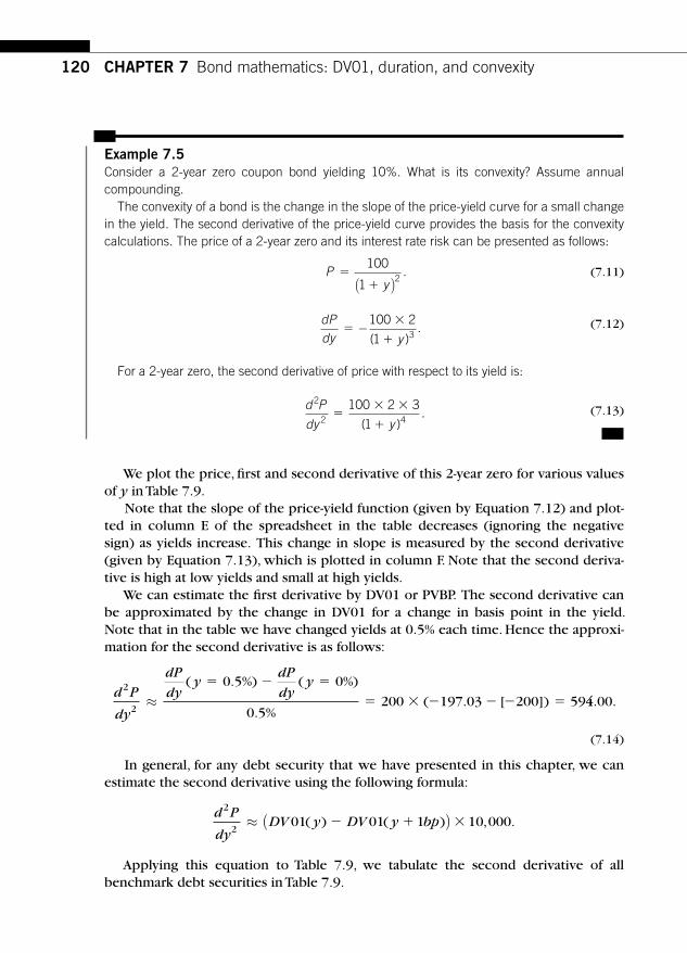
120 CHAPTER 7 Bond mathematics: DV01, duration, and convexity
Example 7.5 Consider a 2-year zero coupon bond yielding 10%. What is its convexity? Assume annual compounding.
The convexity of a bond is the change in the slope of the price-yield curve for a small change in the yield. The second derivative of the price-yield curve provides the basis for the convexity calculations. The price of a 2-year zero and its interest rate risk can be presented as follows:
Py
��
100
12( )
. (7.11)
dPdy y
��
�−
100 2
1 3( ). (7.12)
For a 2-year zero, the second derivative of price with respect to its yield is:
d P
dy y
2
2 4
100 2 3
1�
� �
�( ). (7.13)
We plot the price, fi rst and second derivative of this 2-year zero for various values of y in Table 7.9 .
Note that the slope of the price-yield function (given by Equation 7.12) and plot-ted in column E of the spreadsheet in the table decreases (ignoring the negative sign) as yields increase. This change in slope is measured by the second derivative (given by Equation 7.13), which is plotted in column F. Note that the second deriva-tive is high at low yields and small at high yields.
We can estimate the fi rst derivative by DV01 or PVBP. The second derivative can be approximated by the change in DV01 for a change in basis point in the yield. Note that in the table we have changed yields at 0.5% each time. Hence the approxi-mation for the second derivative is as follows:
d P
dy
dP
dyy
dP
dyy2
2
0 5 0
0 5200 197 03 200 59≈
( . %) ( %)
. %( . [ ])
� � �
� � � � � � 44 00. .
(7.14)
In general, for any debt security that we have presented in this chapter, we can estimate the second derivative using the following formula:
d P
dyDV y V y bp
2
201 01 1 10 000≈ ( )( ) ( ) , .� � �D
Applying this equation to Table 7.9 , we tabulate the second derivative of all benchmark debt securities in Table 7.9 .

1217.4 Convexity
By Taylor series approximation (only using the linear and quadratic terms), we can express the percentage price change as follows:
dP
P
dP
dydy
d P
dydy≈ � 0 5
2
22. ( ) . (7.15)
Using the defi nition of modifi ed duration and moving the price from the denomi-nator on the left side to the right side, we get:
dP P MD dy Pd P
dydy≈ � � � � � �0 5
2
22. ( ) . (7.16)
Table 7.9 Estimating Convexity

122 CHAPTER 7 Bond mathematics: DV01, duration, and convexity
The price change of a debt security, according to Equation 7.16, consists of two terms. The fi rst term is the duration effect, and it is negative. As the yields increase, prices decline. Note that the convexity effect on price change is positive as seen from the sign of the second term. This is referred to as the gain from convexity. We can explicitly compute gain from convexity using the PVBP estimates as shown in Table 7.10 .
We fi nd that the convexity contributes favorably to the price change. Holding maturity and yield to maturity fi xed, the convexity decreases as the coupon increases. Convexity increases with duration.
7.4.1 Bullet versus barbell securities (butterfl y trade)
Let’s consider Table 7.10 and examine the following trading strategy. Is it possible to replace a 5-year T-note with a portfolio of a 2-year T-note and a 10-year T-note such that (a) there is no cash outlay and (b) the PVBP remains the same? If so, what is the difference between these two positions?
A long position in 5-year T-note is a bullet position. A long position in a portfolio of a 2-year T-note and a 10-year T-note is a barbell position, refl ecting the two balloon payments.
Let n2 be the par value of the 2-year T-note and let n10 be the par value of the 10-year T-note needed to replace $100 million par value of a 5-year T-note. We require that the cash proceeds from the sale of a 5-year T-note to be suffi cient to buy the requisite numbers of 2-year and 10-year T-notes. This is the self-fi nancing condition.
n P n P2 2 10 10 100� � . (7.17)
We further require that the DV01 of the 5-year T-note that is sold is equal to the PVBP of the portfolio that is purchased.
n PVBP n PVBP PVBP2 2 10 10 5100� � . (7.18)
Table 7.10 Gain from Convexity
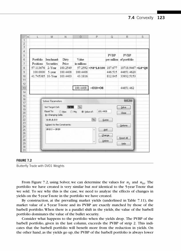
123
From Figure 7.2 , using Solver, we can determine the values for n2 and n10 . The portfolio we have created is very similar but not identical to the 5-year T-note that we sold. To see why this is the case, we need to analyze the effects of changes in yields on the 5-year T-note in the portfolio we have created.
By construction, at the prevailing market yields (underlined in Table 7.11 ), the market value of a 5-year T-note and its PVBP are exactly matched by those of the barbell portfolio. When there is a parallel shift in the yields, the value of the barbell portfolio dominates the value of the bullet security.
Consider what happens to the portfolio when the yields drop. The PVBP of the barbell portfolio, given in the last column, exceeds the PVBP of strip 2. This indi-cates that the barbell portfolio will benefi t more from the reduction in yields. On the other hand, as the yields go up, the PVBP of the barbell portfolio is always lower
7.4 Convexity
FIGURE 7.2
Butterfl y Trade with DV01 Weights

124 CHAPTER 7 Bond mathematics: DV01, duration, and convexity
than that of the 5-year T-note. As a consequence, the barbell portfolio will lose less value compared to the bullet position.
Trades of this sort, in which an intermediate maturity security is sold (bought) and two securities whose maturities straddle the intermediate maturity are bought
Table 7.11 Effect of Convexity, Barbell versus Bullet

1257.5 Effective duration and effective convexity
(sold), are known as butterfl y trades. To get a better perspective, we have plotted in Figure 7.3 the amount by which the value of the barbell portfolio exceeds the value of the 5-year T-note at different levels of yield.
Note that the convexity effect really kicks in only at very high or very low yield levels. In fact, for a �100 basis point change in yields, the effect of convexity is hardly evident. A critical assumption we have maintained throughout this discussion is that the shift in yields is parallel. This assumption is especially suspect when there is a large change in the levels of the yields. Hence, the analysis presented previously should not be construed to mean that convexity is necessarily a desirable attribute.
7.5 EFFECTIVE DURATION AND EFFECTIVE CONVEXITY In our analysis of interest rate risk, we have maintained an assumption that cash fl ows of debt securities are unaffected by changes in market interest rates. Thus in computing DV01, duration, and modifi ed duration, we have assumed that cash fl ows do not change when interest rates change. In a number of circumstances, the cash fl ows of debt securities may depend on interest rate. Callable bonds and MBS are two obvious examples. In such situations, we need to use a concept that refl ects the fact that cash fl ows might change when interest rates change. One such measure is known as effective duration. Another important consequence of the sensitivity of cash fl ows of some debt securities to interest rates is that the concept of yield to
Barbell Value over Bullet0.0450
0.0350
0.0250
0.0200
0.0150
0.0100
0.0050
0.0000
0.0400
0.0300
3.560% 3.760% 3.960% 4.160% 4.360% 4.560% 4.760% 4.960%
Yield scenarios
Val
ue o
f con
vexi
ty
FIGURE 7.3
Barbell versus Bullet
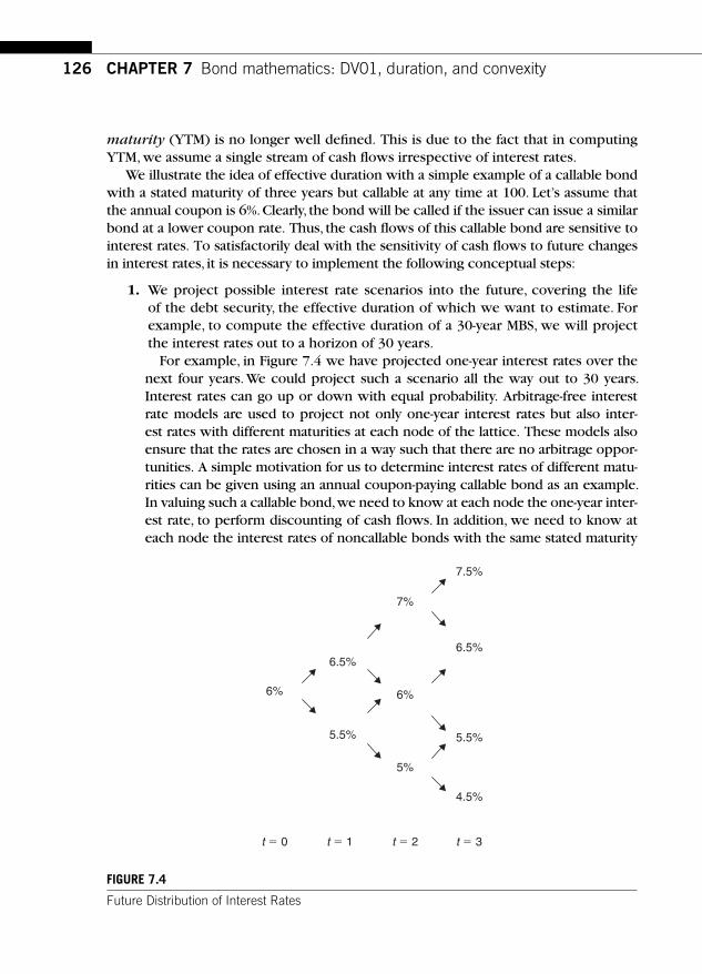
126 CHAPTER 7 Bond mathematics: DV01, duration, and convexity
maturity (YTM) is no longer well defi ned. This is due to the fact that in computing YTM, we assume a single stream of cash fl ows irrespective of interest rates.
We illustrate the idea of effective duration with a simple example of a callable bond with a stated maturity of three years but callable at any time at 100. Let’s assume that the annual coupon is 6%. Clearly, the bond will be called if the issuer can issue a similar bond at a lower coupon rate. Thus, the cash fl ows of this callable bond are sensitive to interest rates. To satisfactorily deal with the sensitivity of cash fl ows to future changes in interest rates, it is necessary to implement the following conceptual steps:
1. We project possible interest rate scenarios into the future, covering the life of the debt security, the effective duration of which we want to estimate. For example, to compute the effective duration of a 30-year MBS, we will project the interest rates out to a horizon of 30 years. For example, in Figure 7.4 we have projected one-year interest rates over the next four years. We could project such a scenario all the way out to 30 years. Interest rates can go up or down with equal probability. Arbitrage-free interest rate models are used to project not only one-year interest rates but also inter-est rates with different maturities at each node of the lattice. These models also ensure that the rates are chosen in a way such that there are no arbitrage oppor-tunities. A simple motivation for us to determine interest rates of different matu-rities can be given using an annual coupon-paying callable bond as an example. In valuing such a callable bond, we need to know at each node the one-year inter-est rate, to perform discounting of cash fl ows. In addition, we need to know at each node the interest rates of noncallable bonds with the same stated maturity
7.5%
6.5%6.5%
5.5% 5.5%
4.5%
5%
6%6%
7%
t � 0 t � 1 t � 2 t � 3
FIGURE 7.4
Future Distribution of Interest Rates

127
as the callable bond. This latter information will be used in determining whether the bond should be called or not. Likewise, in valuing a mortgage, we need to project monthly interest rates at each node for discounting. In addition, we also need to project refi nancing rates at each node to evaluate the value of prepaying the mortgage. Finally, we need to make sure that the refi nancing rates and one-month interest rates are chosen so as to preclude arbitrage. We assume that the yield curve is fl at at each node. Then, it is clear that the bond will be called at all nodes where the interest rates are lower than 6%.
2. Next we select a random path of interest rates. In Figure 7.5 we show a possi-ble path of interest rates, which are highlighted. The highlighted interest rates over time are the result of a randomly chosen interest rate path over the next three years. One way to choose a random path is to fl ip a (fair) coin at date t � 0. If the result is heads, we go up; otherwise, we move down. We repeat this process a suffi cient number of times to generate a path.
3. Next we estimate the cash fl ows along that path. For a callable bond, when interest rates go down, the bond may be called. For a mortgage, when refi -nancing rates go down, mortgages may be prepaid. So, at each node, cash fl ows will refl ect the optimal behavior of bond issuers (in the case of call) or investors (in the case of mortgages). The result will be a set of cash fl ows at each node, as shown in Figure 7.6 . We assume that the bond starts to pay cash fl ows from t � 1 and matures at t � 3. Note that the bond will be called at t � 1, and the investors will receive the par value of 100 and the coupon of 6. The bond’s cash fl ows along the interest rate path are 106 at date 1 and zero at other dates on the simulated path.
7.5 Effective duration and effective convexity
7.5%
6.5%6.5%
5.5% 5.5%
4.5%
5%
6%6%
7%
t � 0 t � 1 t � 2 t � 3
FIGURE 7.5
Simulation of an Interest Rate Path

128 CHAPTER 7 Bond mathematics: DV01, duration, and convexity
4. Next we estimate the present value of cash fl ows along each simulated path. Since we know the one-year interest rates and annual cash fl ows, we can dis-count the cash fl ows and compute the present value of cash fl ows. In the exam-ple, the present value is simply 100/1.06 � 100. In this manner we can computethe present values of many simulated paths. Note that when simulated paths have nodes with interest rates higher than 6%, we need to compute the pres-ent values, recognizing that the bond will not be called at those nodes and will just pay the promised coupons.
5. Next we compute option-adjusted spreads (OASs). Once we have the present values of all simulated paths, we average all the present values. If the average present value across all simulated paths is exactly equal to the market price, we defi ne the OAS as zero. If the average of present values is higher than the mar-ket price, we add a constant spread z to the discount rate at each node until the average is equal to the market price. This spread z is defi ned as the OAS.
6. Finally, we compute effective duration. Let’s denote the market price as P. We increase interest rates at all nodes by a certain amount (say, 10 basis points) and recompute the price, holding the OAS fi xed. Let’s denoted this price as P�. Then we recalculate the price by decreasing the interest rates at all nodes by 10 basis points. Let’s denote this price as P�. Then the effective duration for a 1% change in interest rates is calculated as follows:
( ) .P P� �� � 5
106 0
0
t � 0 t � 1 t � 2 t � 3
FIGURE 7.6
Cash Flows of a Callable Bond Along the Simulated Path

129
The reason that we multiply the price change by 5 is simple: The price dif-ference is over a 20-basis-point overall change. So, multiplying by 5 gives an estimate of the price change for a 100-basis-point change. The effective dura-tion takes into account the effect of changes in interest rates on cash fl ows.
The calculation of effective convexity is also direct and similar to the way we computed convexity earlier. We fi rst compute the price change for a 10-basis-point decrease. We then compute the price change for a 10-basis-point increase. We take the difference between these two price changes to get a measure of effective convexity.
Figure 7.7 illustrates the prices at different yields and the way effective duration and convexity measures work. One point worth remembering is that effective duration and effective convexity measures are functions of the models used to compute OAS. Different models (with differing assumptions) can produce differing estimates of effec-tive duration and convexity. We review some of the models of interest rates in Chapter 9 so that the reader is aware of the underlying assumptions behind such models.
Sometimes the OAS is changed by 10 basis points to recalculate the price. Then this price and the original market price are used to estimate spread duration. Such calculations are useful for securities such as corporate debt securities, which trade at a spread over Treasuries.
SUGGESTED READINGS AND REFERENCES Kopprasch , B. ( 2004 ) . A look at a variety of duration measures . United States Fixed Income
Research , Solomon Smith Barney, Citigroup .
Suggested readings and references
P �
P �
P
Effective duration � (P� � P�) � 5
Effective convexity � [(P� � P ) � (P � P�)] � 5
Interest rates
Pric
es
FIGURE 7.7
Illustration of Effective Duration and Convexity

This page intentionally left blank

131
CHAPTER
Fixed Income Markets and Their DerivativesCopyright 2009 by Academic Press. Inc. All rights of reproduction in any form reserved.
8 CHAPTER SUMMARY In this chapter the concept of yield curve and the three types of risks that are pres-ent in the yield curve are illustrated: level risk, slope risk, and curvature risk. We describe the differences between price volatility and yield volatility. The chapter presents evidence that short-term interest rates are typically much more volatile than long-term yields. The concept of term structure of interest rates is introduced, and tools such as the spot rates of interest, forward rates of interest, and par bond yield curves are developed and illustrated with specifi c real-life examples. We show how coupon bonds can be built as a portfolio of zero coupon bonds. We explain strips and implied zeroes and develop the economics that underlie stripping cou-pon-paying bonds and reconstitutions of strips into coupon bonds.
8.1 YIELD-CURVE ANALYSIS Yield curve is a term used to describe the plot of yield to maturity against time to maturity or against a risk measure, such as the modifi ed duration of debt securities in a certain market segment (such as Treasury or corporate bonds). It is therefore natural to speak of “Treasury yield curve ” or “corporate AAA yield curve. ” By incor-porating the expectations of diverse participants in the marketplace, the shape of the yield curve succinctly captures and summarizes the cost of credit for various maturities of different issuers. The shape of the default-free yield curve is, therefore, of considerable interest to practitioners in the fi nancial markets. To get some basic understanding of this concept, we plot the yield to maturity along the Y axis and time to maturity along the X axis using all 160 Treasury debt securities that were outstanding for settlement on July 11, 2008. Figure 8.1 shows the resulting plot of the yield curve as of that date.
Yield curve and the term structure

132 CHAPTER 8 Yield curve and the term structure
Several features of the yield curve are worth noting. First, note the sparseness of yield data for maturities in the range 2029 through 2035. This is due to the fact that 30-year T-bond auctions were cancelled during the period March 2001 to January 2006 and were only resumed in February 2006. Second, the yield curve is relatively fl at in the far end (longer maturity sector) and somewhat steep in the front maturities. Finally, we note that there are some debt securities whose yields plot well outside the general area around which the yields have clustered. Even within the same maturity range, yields tend to differ. Some of the outstanding debt issues were callable, and not surprisingly these were trading at a higher yield. We explore this activity later in the chapter.
Recall that the concepts of duration and convexity are strictly valid only when the movements in the yield curve are parallel. What is the meaning of a parallel shift in yield curve? Consider Table 8.1 , which records yield to maturity of selected benchmarks in the Treasury market. The yield to maturities of the benchmarks on November 8, 1979, are shown. These are plotted in Figure 8.2 . Suppose all the yields moved up by 0.50%. The resulting shift is called parallel and is shown by the dashed curve in Figure 8.2 .
How realistic is the parallel shift assumption? To examine this question, we begin by presenting the shape of the yield curve at selected points in time and noting the observed shifts in the shape of the yield curve over time.
Note the sharp differences in (a) levels of interest rates, (b) slope of the yield curve, and (c) the overall shape of the yield curve. On November 8, 1979, inter-est rates were rather high and short-term interest rates were higher than long-term interest rates, producing an inverted yield curve . In fact, the spread between 30-year yields and 2-year yields was � 178 basis points. This is shown in Figure 8.2 .
By October 9, 1992, the levels had fallen signifi cantly: Two-year yields stood at 4% and 30-year yields at 7.52%. The spread between 30-year yields and 2-year yields was �352 basis points, resulting in an upward-sloping yield curve, as illustrated in Figure 8.3 .
6.000
5.000
4.000
3.000
2.000
1.000
10.00 15.00 20.00 25.00 30.00 35.000.000
YT
M
0.00 5.00
Time to maturity in years
Yield curve on July 11, 2008
FIGURE 8.1
Treasury Yield Curve Quoted as of July 11, 2008 Source: Wall Street Journal.

133
Finally, on November 9, 1999, the yield curve was “ humped ” in the sense that the yields increased as the maturity increased from two to seven years. Then the yield dropped below the seven-year level, as illustrated in Figure 8.4 .
Table 8.1 and Figures 8.2 – 8.4 vividly illustrate three different types of risk: (a) levels of interest rates, (b) slope of the yield curve, and (c) shape of the yield curve.These three variables ( level, slope, and curvature) have been found extremely useful in explaining the variations in yield curve.
To get an idea of the risk associated with the slope risk in the yield curve, exam-ine Figure 8.5 , where the spread between the 10-year yields and 2-year yields are plotted for the 30-year period 1977 – 2008.
The spread shown in Figure 8.5 is a good proxy for the slope risk. It reached a low of �250 basis points in early 1980s and touched a maximum of �250 basis points.
Table 8.1 Yield Curve as of Three Dates, 1979 – 1999
Benchmark Maturity November 8, 1979 October 9, 1992 November 9, 1999
YTM YTM YTM
2 12.29 4.00 5.77
3 11.67 4.50 5.81
5 11.28 5.50 5.87
7 11.10 6.08 6.10
10 10.96 6.52 5.97
30 10.51 7.52 6.07
Source : The Board of Governors of the Federal Reserve.
10.50
11.00
11.50
12.00
12.50
13.00
0 5 10 15 20 25 30 35
CMT yields – inverted yield curve
Yield to maturity
Parallel shift up
FIGURE 8.2
Yield Curve as of November 8, 1979 Source: The Board of Governors of the Federal Reserve.
8.1 Yield-curve analysis

134 CHAPTER 8 Yield curve and the term structure
Note that periodically the yield curve becomes inverted: August 1978 to April 1980, September 1980 to October 1981, and January 1982 to July 1982 all saw signifi cant inversion. Less severe inversions occurred during 1989 and during February 2000 to December 2000. Figure 8.5 shows that nonparallel shifts appear to be pervasive.
In this discussion, we have chosen to work with data for specifi c maturities: 3 months, 6 months, 1 year, 2 years, 3 years, 4 years, 5 years, 7 years, 10 years, 15 years, 20 years, and 30 years. In reality, there are about 160 Treasury securities that are outstanding in the marketplace, ranging in maturity from a few days to 30 years. This presents a challenge to practitioners and researchers as outstanding debt varies in terms of (a) coupon, (b) vintage (when they were issued), (c) callability, and so on.
8.00
7.50
7.006.50
6.00
5.50
5.00
4.50
4.000 5 10 15 20 25 30 35
Time to maturity in years
YT
M
CMT yields – normal yield curve
FIGURE 8.3
Yield Curve as of October 9, 1992 Source: The Board of Governors of the Federal Reserve.
6.156.106.05
6.005.955.905.855.805.75
YT
M
0 5 10 15 20 25 30 35
Time to maturity in years
CMT yields – humped yield curve
FIGURE 8.4
Yield Curve as of November 9, 1999 Source: The Board of Governors of the Federal Reserve.

135
8.1.1 Principal components analysis of yield curves
The foundation of principal components analysis (PCA), developed by Karl Pearson, has been applied to develop a better appreciation of yield curves by Litterman and Scheinkman (1991) . The PCA approach recognizes that the interest rates of various maturities (zero yields) are very likely correlated with a relatively small number of underlying economic variables that cannot be observed directly. Such unobserved economic variables are known as latent variables. For example, zero yields of var-ious maturities are all correlated with each other. Economic intuition would then suggest that perhaps a few (three or four) common latent variables drive them all. It then stands to reason that the observed correlation matrix of zero yields may be used to draw some inferences about the identities of such latent variables. PCA pre-sents a systematic analysis of observed correlations among market yields to identify underlying latent principal components.
PCA identifi es independent factors that explain the maximum amount of observed correlation among yields. PCA begins by assuming that there are as many latent vari-ables (principal components) as there are zero variables. So, if we start with fi ve benchmarks (say, fi ve zero yields: 2-year, 3-year, 5-year, 10-year, and 30-year), PCA assigns fi ve latent variables. Litterman and Scheinkman (1991) performed a PCA on gov-ernment yield curve and concluded that there are three major principal compo-nents that can help explain the comovements of yields of various maturities. They associated these three latent variables with (a) level of interest rates, (b) steepness of yield curve, and (c) the convexity of the yield curve or its curvature. Table 8.2 is reproduced from their paper. They conclude that considering explicitly these three variables in hedging interest rate risk is likely to produce much better outcomes than simply holding a zero duration position.
CMT yield spreads – 10-year minus 2-year yields
�250
�150
�50
50
150
250
F-77
1977–2008
Spr
ead
in b
asis
poi
nts
M-07J-04S-01J-99A-96J-93O-90J-88A-85J-82N-79
FIGURE 8.5
Slope of Yield Curve, 1977 – 2008 Source: The Board of Governors of the Federal Reserve.
8.1 Yield-curve analysis

136 CHAPTER 8 Yield curve and the term structure
Researchers in this area have found that the fi rst component explains about 90–95% of the variations. The second component helps explain an additional 4 –7%of the variation, so that taken together, two components can explain nearly 95 –98%of the changes in daily yields. The third component picks up much of the remaining variations. They also show that the effect of the fi rst component is roughly constant across yields of all maturities. To hedge this component, duration-based strategies will do a decent job. The second component pushes down the yields of 1 to 5 years but increases the rest of the yields up to nearly 20 years. The fi nal component is related to interest rate volatility. Roughly similar conclusions emerge when PCA is performed on swap rates of various maturities.
To get additional insights into the shape of the yield curve and the pattern of its changes, we need to examine the volatility of short-term and long-term interest rates.
8.1.2 Volatility of short and long rates
Volatility measures the variability of interest rates relative to their expected average levels. Loosely speaking, volatility measures the degree of variation of any variable around its mean. Given historical observations, we can estimate the volatility. It stands to reason that the degree of variation, as well as the mean of the interest rates, changes with time as the economic determinants of interest rates change. For example, the short rates of interest changed signifi cantly between 1978 and 1983. This was, in large part, due to a change in the monetary policy that was effected by the Fed. (This is an extreme example in the sense that the entire structure underlying
Table 8.2 PCA of Implied Zero Yields: Relative Importance of Factors (%)
Maturity Total Variance Explained
Proportion of Total Explained —Variance Accounted for by:
Factor 1 Factor 2 Factor 3
6 months 99.5 79.5 17.2 3.3
1 year 99.4 89.7 10.1 0.2
2 years 98.2 93.4 2.4 4.2
5 year s 98.8 98.2 1.1 0.7
8 years 98.7 95.4 4.6 0.0
10 years 98.8 92.9 6.9 0.2
14 years 98.4 80.5 14.3 5.2
18 years 95.3 80.5 8.5 2.0
Average 98.4 89.5 8.5 2.0
Source: Robert Litterman and Jose Scheinkman, “Common Factors Affecting Bond Returns, ” Journal of Fixed Income, June 1991.

137
interest rates was affected.) The levels of interest rates and their volatility might sys-tematically incorporate the changes in the factors that affect them. As a consequence, the time series of interest rates might exhibit a systematic clustering effect. The esti-mation procedures used for volatility vary signifi cantly in their levels of sophistica-tion. Some do not explicitly account for the fact that the volatilities exhibit clustering effects; others do. Figure 8.6 shows the volatility of 2-year and 10-year constant matu-rity yields during the period 1977 to 1982. Figure 8.7 provides the same information for the period 1998 to 2008.
Long-term and short-term volatilities
0.00%
5.00%
10.00%
15.00%
20.00%25.00%
30.00%
35.00%
40.00%
45.00%
21-Jul-76
1977–1982
26-May-8311-Jan-8229-Aug-8017-Apr-7903-Dec-77
Two-year volatility
Ten-Year volatility
FIGURE 8.6
Short-Term and Long-Term Interest Rate Volatilities, 1977 – 1982
Volatility of Short-term and long-term yields
1.00%
3.00%
5.00%
7.00%
9.00%
11.00%
13.00%
15.00%
20-Aug-97
1998–2008
Vol
atili
ty
Two-year volatility
Ten-Year volatility
18-Feb-0921-Mar-0720-Apr-0521-May-0320-Jun-0121-Jul-99
FIGURE 8.7
Short-Term and Long-Term Interest Rate Volatilities, 1998 – 2008
8.1 Yield-curve analysis

138 CHAPTER 8 Yield curve and the term structure
Volatilities were estimated based on 20 days of rolling observations. Note the dra-matic fall in volatility in the latter period, during which the volatility was well within 15%. During the period June 2003 through early 2007, volatility dropped rather sig-nifi cantly, to nearly 5% or less. The onset of a credit crunch in August 2007 increased the interest rate volatility to over 13%.
8.1.3 Price-based versus yield-based volatility
It is useful to distinguish between price-based and yield-based volatilities in the con-text of fi xed-income securities markets. The prices of fi xed income securities tend to par as their maturity dates approach. The price-yield relation that we developed earlier can be used to derive one volatility, given the other. For example, we showed that the modifi ed duration is given by
MDdP
dy P� �
1 (8.1)
We can estimate the price volatility using historical data on price changes or on yield changes. Equation 8.1 makes it clear that price volatility and yield volatility are related through the modifi ed duration of the debt security. Though short-term yields are generally more volatile than long-term yields, long-term bond prices are much more volatile than short-term debt securities, which pay par value at maturity and hence cannot trade too far away from par. In pricing options on bonds, bond price volatility is more important; on the other hand, in pricing options on yields, it is the volatility of yields that is more relevant.
When we examine the volatility of interest rates of various maturities, we note that the short-term rates are much more volatile than long-term rates. This consid-eration is important for several reasons. First, in the specifi cation of a satisfactory model of the term structure, it is necessary to incorporate this feature of interest-rate volatility. Second, the pricing and hedging of many interest rate derivative products are signifi cantly infl uenced by the volatility, and it is important to incorporate the dif-ferential volatility of short-term and long-term interest rates in their valuation.
8.1.4 Economic news announcements and volatility
Economic news arrives in a lumpy fashion in capital markets. In equity markets, compa-nies announce their earnings every quarter. Market participants form expectations about earnings, and actual earnings may produce either a positive or negative surprise relative to expectations. Such surprises may result in positive or negative jumps in stock prices and can result in a jump in volatilities. In his examination of Treasury yields, Johannes (2004) fi nds that jump times and sizes are related to surprises about macroeconomic news. He fi nds that jumps are more relevant in pricing interest rate derivatives than bonds. In fi xed income markets, broad news announcements occur periodically, and their effects on yields, bid-offer spreads, and volatilities have been explored by Balduzzi, Elton, and Green (2001) . They examined news announcements and their effects on Treasury securities and documented the news announcements outlined in Table 8.3 .

139
Table 8.3 Economic News Announcements in Bond Markets
8:30 a.m. Announcements
9:15 a.m. Announcements
10:00 a.m. Announcements
2:00 p.m. Announcements
4:30 p.m. Announcements
1. Civilian unemployment(% level)
13. Capacity utilization (% level)
15. Business Inventories (% change)
23. Treasury budget (change in $ billions)
24. Money supply measures: M1, M2, and M3
2. Consumer price index (% change)
14. Industrial production (% change)
16. Construction spending (% change)
3. Durable Goods orders (% change)
17. Consumer confi dence (% level)
4. Housing starts (millions of units)
18. Factory orders (% change)
5. Index of leading indicators (% change)
19. NAPM Index (index value)
6. Initial jobless claims, weekly (thousands)
20. New home sales (in thousands)
7. Merchandise trade balances ($ billions)
21. Personal consumption (% change)
8. Nonfarm payrolls (change in thousands)
22. Personal income (% change)
9. Producer price index (% change)
10. Retail sales (% change)
11. U.S. imports ($ billions)
12. U.S. exports ($ billions)
Source : Balduzzi, Elton, and Green, “ Economic News and Bond Prices: Evidence from the U.S. Treasury Market, ” The Journal of Financial and Quantitative Analysis , Vol. 36, No. 4, (December 2001), pp. 523 – 543.
8.1 Yield-curve analysis

140 CHAPTER 8 Yield curve and the term structure
Balduzzi, Elton, and Green (2001) used data on bid and ask quotes, trade prices, and trading volume for Treasury bills, notes, and bonds in the interdealer broker market (GovPX) for the period July 1, 1991, to September 29, 1995. They found that surprises in news announcements (as measured by deviations from forecasts) can explain a sub-stantial fraction of price volatility that follows announcements. Markets are generally very fast in adjusting to news: It takes less than one minute for the adjustment to occur. Volatility and trading volume increase signifi cantly after the announcements. To sum up, bond yields and their volatilities depend on many factors, including (a) maturity, (b) business cycles, and (c) surprises in economic news announcements.
8.1.5 Yield versus duration
The yield curve, as mentioned earlier, is the plot of yield to maturity as a function of time to maturity. We can plot the yield versus modifi ed duration. Figure 8.8 depicts the yield curve on July 11, 2008.
All Treasury notes and bonds that were outstanding for settlement on July 11, 2008, are represented in Figure 8.8 . To illustrate the problems of drawing sensible inferences from this yield curve, we should note fi rst that of the nearly 160 Treasury notes and bonds that were outstanding in the market, a few were callable by the Treasury at par on any coupon day during the last fi ve years of the bond’s stated life. This feature will infl uence their yields.
8.1.6 Coupon and vintage effects
In each duration range, there are clusters of Treasury securities of varying vintages, coupons, and contractual provisions, as illustrated in Table 8.4 .
5.000
4.500
4.000
3.500
3.000
2.500
2.000
1.500
1.0000.000 2.000 4.000 6.000 8.000 10.000 12.000 14.000 16.000
Modified duration
Yield to maturity versus modified durationY
ield
to m
atur
ity
FIGURE 8.8
Yield Versus Modifi ed Duration, as of July 11, 2008 Source: The Wall Street Journal .

141
Note, for example, in the duration bucket 10 to 17 years there are debt securities, which are more than 13 years old, and there are newly issued securities. This “ vin-tage ” problem is even more severe in the duration buckets 5 to 10 and 2 to 5. Many callable 30-year bonds with fairly high coupons, which were issued 25 years ago, are still outstanding. The range of yields in these duration buckets is very large. The dif-ferences in yields can be very substantial, even for securities maturing on exactly the same date, as shown in Table 8.5 .
Some of the yield differences are accounted for by the fact that high-coupon bonds in Table 8.5 (12% and 9.125%) were callable.
Table 8.4 Diversity of Coupons and Vintage Effects in Yield Curve as of July 11, 2008
Modifi ed Duration Range
YTM Range Coupon Range Vintage Range in Years
Max Min Max Min Max Min
0 to 1 2.918% 1.016% 5.500% 2.625% 1.115 0.948
1 to 2 2.627% 2.326% 6.500% 1.750% 8.910 0.030
2 to 5 4.898% 2.285% 13.250% 2.500% 24.923 0.030
5 to 10 4.497% 3.380% 10.625% 3.500% 24.173 0.068
10 to 17 4.606% 4.489% 7.625% 4.375% 13.915 0.403
Table 8.5 Vintage Effects for Identical Maturity Dates as of July 11, 2008
Issue Date Maturity Date Coupon Rate YTM
08/15/03 08/15/08 3.250 1.016
08/15/05 08/15/08 4.125 1.078
Yield difference in basis points: 6.20
08/16/04 08/15/09 3.500 2.423
08/15/06 08/15/09 4.875 2.450
Yield difference in basis points: 2.70
8/7/03 8/15/13 4.250 3.249
8/15/83 8/15/13 12.000 4.898
Yield difference in basis points: 164.90
06/16/08 05/15/18 3.875 3.940
05/16/88 05/15/18 9.125 4.063
Yield difference in basis points: 10.23
8.1 Yield-curve analysis

142 CHAPTER 8 Yield curve and the term structure
Note that the yield differences are well outside the bid-offer spread and, hence, are of economic signifi cance. Table 8.5 gives anecdotal evidence to the effect that high-coupon securities tend to trade at a slightly higher yield. One possible explanation is that many institutional investors with long-dated liabilities might prefer low-coupon securities, which tend to have a longer duration. As noted in Chapter 7, higher dura-tion means a higher sensitivity to interest rates. Such assets may be ideal to match the interest rate sensitivity of long-dated liabilities. Pension funds and insurance compa-nies are examples of such institutional investors. They may drive up the price of low-coupon securities, thereby bringing down their yields. There may be tax considerations as well. High-coupon bonds that pay higher interest may subject certain investors to a greater tax exposure. If such investors are the marginal holders of these bonds, they may demand a higher yield. Conversely, low-coupon bonds may be accepted at a lower yield. The regulatory restrictions faced by institutions could also play a part. In Japan, certain institutions are not permitted to pay dividends from capital gains; they are per-mitted to pay dividends only from interest income. They prefer high-coupon bonds. As a result, high-coupon bonds in Japan have tended to exhibit lower yield in many periods.
The newly issued securities (the on-the-run issues) tend to be more liquid; we showed evidence of this in Chapter 1. As such, they will sell at a higher price. In other words, they command a liquidity premium, whereas off-the-run issues will be cheaper, ceteris paribus, because of their illiquidity. Warga (1992) shows that recently issued bonds (on-the-run) are priced to refl ect a premium of about 55 basis points per annum compared to otherwise identical bonds. Table 8.6 , taken from
Table 8.6 Differences in YTM of On-the-Run and Off-the-Run Treasury Debt
Duration Range (Months) Mean Difference in YTM in Basis Points ( t -Statistics in Parenthesis)
20 to 24 47.60 (3.5)
28 to 32 40.60 (2.4)
36 to 40 55.90 (4.1)
40 to 44 38.50 (1.6)
44 to 48 65.20 (3.5)
48 to 52 131.00 (5.3)
56 to 60 7.16 (0.25)
60 to 64 101.00 (3.1)
64 to 72 56.50 (1.9)
72 to 84 8.67 (0.2)
Source : Warga, “Bond Returns, Liquidity, and Missing Data, ” Journal of Financial and Quantitative Analysis , 1992, 27 (4), pp. 605 –617.

143
Warga’s paper, vividly illustrates that off-the-run issues are priced at a discount rela-tive to on-the-run issues across a duration range of 20 to 84 months.
The evidence presented should not be interpreted to imply that there are arbi-trage opportunities; we saw in Chapter 5 that on-the-run issues have more attractive borrowing rates (they trade “ special ” in repo markets). The important message to take away from the evidence is that the yield curve is populated by many debt issues with varying vintage, coupons, and contractual features. These debt issues may differ in liquidity. Some of them may trade at a discount and some at a premium above par. For pricing purposes, we need a good benchmark at each maturity date clearly indi-cating the yield at that maturity date. Ideally, we would like to price a zero coupon bond at each maturity. With so many variations in vintages and coupons, it is very diffi cult to estimate the correct yield for a zero coupon bond at any given maturity date. In addition, there are some maturity dates for which no issues are present in the market. For example, as noted earlier, Treasury suspended the auctions of 30-year T-bonds during 2001 –2006. This action resulted in maturity sectors for which we have no yields. To develop estimates of yields at those maturities, we need a theoreti-cal benchmark as well. This leads us to the concept of term structure.
8.2 TERM STRUCTURE To develop a sharp intuition about the shape of the yield curve and the factors that underlie the levels and the shape, we need a more parsimonious representation of the yield curve than Figure 8.1 . It is in this context that we defi ne the term structure of interest rates.
Term structure of interest rates refers to the relationship between the yield to maturity of default-free zero coupon securities and their maturities.
Often the yield to maturity on a default-free zero coupon (pure discount) bond is termed the spot rate of interest. The relationship between the spot rate of a pure discount bond and its maturity is referred to as the spot curve. To get a better handle on the pricing of zero coupon bonds, we fi rst develop the pricing principles for a default-free pure discount bond.
8.2.1 Implied zeroes
The concept of term structure is best developed in terms of pure discount bonds or zero coupon bonds. We defi ne the notation for the price of a zero, suggested earlier, more formally as zj , the price of a pure discount bond today that pays $1 in j periods from now. If we set j � 2, then z 2 will represent the price of a two-year zero coupon bond. We assume that the discount bonds are free from default risk. (The treatment of credit risk requires the modeling of economic factors that lead to fi nancial dis-tress and of the negotiations between creditors and borrowers in times of fi nancial distress. In addition, such factors as liquidation costs and cash-fl ow generating capac-ity of the borrower become relevant. We consider credit risk in detail in Chapter 10.)
8.2 Term structure

144 CHAPTER 8 Yield curve and the term structure
Examples of default-free zero coupon securities are T-bills (considered in Chapter 2) and zero coupon securities obtained by stripping U.S. Treasury securities. The analy-sis of strips is taken up later in this chapter.
8.2.2 Bootstrapping procedure
Spot rates are associated with specifi c maturities. Thus, the spot rate yj for a pure dis-count bond maturing j years from now may be defi ned as the discount rate at which the present value of the promised terminal cash fl ow of the pure discount bond is equal to its price. Recall that zj is the price today of a pure discount bond paying $100 in j periods; then
zy
jj
j�
�
100
1( ), (8.2)
where yj is the spot rate of interest on a zero coupon bond with a time to maturity of j.
Often, we are confronted with situations in which the prices of coupon bonds are readily available, but zero coupon prices are diffi cult to get. So, it is necessary to try to estimate zero coupon bond prices based on the prices of coupon bond prices. A procedure known as bootstrapping is used for this purpose. This procedure is illustrated in Example 8.1.
Example 8.1 Consider the problem of fi nding the pure discount bond prices from the coupon bond prices that are available. Table 8.7 gives data for three bonds for a period of three years. Note that Bond 1, which matures in a year’s time, has a coupon of 5% (annual) and is selling at a price of 99.50. Bond 2, which matures two years from now, pays a coupon of 6% (annual) and is selling at a price of 101.25. Finally, Bond 3, which pays a coupon of 7%, matures three years from now and is selling at a price of 100.25.
Let Pi be the price of bond i. Let Ci denote the dollar coupon associated with bond i. Then we can denote the price of the fi rst bond as
PC
y1
1
11
100
1�
�
�( ). (8.3)
Table 8.7 Prices of Coupon Bonds
Bond Price Year 1 Year 2 Year 3
1 99.50 105 0 0
2 101.25 6 106 0
3 100.25 7 7 107

145
We use the information pertaining to Bond 1 from Table 8.7 in Equation 8.3 to get
99 50100 5
1 1.
( ).�
�
� yi
(8.4)
Solving for y 1, we get a one-year spot rate of interest of 5.53% (rounded to two decimals for
reporting). The one-year implied zero is defi ned as
zy
11
1
100
194 76�
��
( ). . (8.5)
In Equation 8.5, we have substituted y 1 � 5.53%. Armed with the knowledge of y 1 we can
determine y 2. To do this, recognize that the price of Bond 2 can be written in terms of the two spot rates of interest as
Py
2 12
2
6
1 0 0553
100 6
1101 25�
��
�
��
( . ) ( ). . (8.6)
Note that the fi rst coupon of 6, which will be paid at year 1, is discounted at the one-year
spot rate of interest. The fi nal payment of 106, paid in year 2, is discounted at the two-year spot rate of interest. We can solve for the two-year spot rate as y 2 � 5.32%. The implied zero for two-year maturity may be found by
z2 2
100
1 0 53290 15�
��
( . ). .
Proceeding in this way, we can determine y
3 and z
3 as well. The price of Bond 3 may be
written as
Py
3 1 23
3
7
1 0 0553
7
1 0 0532
100 7
1100 25�
��
��
�
��
( . ) ( . ) ( ). . (8.7)
Note that in Equation 8.7, the only unknown quantity is y 3, the three-year spot rate of inter-
est. We solve for y 3 as 7.02%. The results are presented in Table 8.8 .
Table 8.8 Implied Zero Prices and Spot Rates
Maturity Implied Zero Price Spot Rate of Interest
1 0.9476 5.53%
2 0.9015 5.32%
3 0.8159 7.02%
We can rewrite the price of three-year coupon bond in Equation 8.7 as
P z z z3 1 2 37 7 107� � � . (8.8)
Recall that zj is the price of a zero today, which pays a dollar j periods from now. Equation 8.8 says that the price of a three-year coupon bond is a portfolio of zero coupon bonds; if we buy seven units of a one-year zero, seven units of a two-year
8.2 Term structure

146 CHAPTER 8 Yield curve and the term structure
zero, and 107 units of a three-year zero, the payoffs of such a portfolio will be identi-cal to the three-year coupon bond in our example.
Note that this example is hypothetical and is intended merely to illustrate the concept of building the spot curve from coupon bonds. In real life, debt securities have coupon and vintage effects, as discussed earlier. In addition, bonds might not be available at every maturity sector. Some maturity ranges are spanned by bonds that are callable. In Table 8.5 we noted that callable bonds dominate the maturity range 2009–2013. So, the problem of building implied zeroes is far from being as simple as is suggested by our example.
Before proceeding to address these important estimation problems, we briefl y state the general relationship between coupon bond prices and spot rates of interest. In Example 8.1, we used the information on coupon bond prices as input to derive the zero coupon bond prices. Such estimates of zero coupon bond prices are known as implied zeroes, since they are implied by coupon bond prices. Let’s denote the cash-fl ow information about coupon bonds as Matrix A:
A �105 0 0
6 106 07 7
107
⎡
⎣
⎢⎢⎢⎢
⎤
⎦
⎥⎥⎥⎥.
Let’s denote by p � [99.50, 101.25, 100.25] the vector of bond prices and let z � [z 1,z 2,z 3] be the vector of zero prices. Then the zero bond prices and the coupon bond prices satisfy the relation p � Az. Note that this notation is a compact math-ematical way of saying that the prices of bonds are the sum of discounted cash fl ows.
We then solve for the zero prices by inverting matrix A:
z A p� �1
This way of extracting implied zero prices from coupon bond prices will be helpful when there are many coupon bonds with regular and uniform maturity intervals , as the next example illustrates.
Example 8.2 Table 8.9 shows the prices of various Treasury securities for settlement on October 9, 1999.
Table 8.9 Coupon Bond Prices
Settlement Date October 9, 1999
Maturity Coupon Price (in 32nds)
Bid Clean Ask Clean
2/15/2000 5.000% 100.05 100.07
8/15/2000 8.000% 103.00 103.02
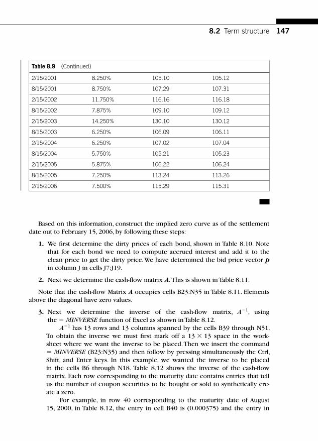
147
Based on this information, construct the implied zero curve as of the settlement date out to February 15, 2006, by following these steps:
1. We fi rst determine the dirty prices of each bond, shown in Table 8.10 . Note that for each bond we need to compute accrued interest and add it to the clean price to get the dirty price. We have determined the bid price vector p in column J in cells J7:J19.
2. Next we determine the cash-fl ow matrix A . This is shown in Table 8.11 .
Note that the cash-fl ow Matrix A occupies cells B23:N35 in Table 8.11 . Elements above the diagonal have zero values.
3. Next we determine the inverse of the cash-fl ow matrix, A � 1, using the � MINVERSE function of Excel as shown in Table 8.12 .
A � 1 has 13 rows and 13 columns spanned by the cells B39 through N51. To obtain the inverse we must fi rst mark off a 13 � 13 space in the work-sheet where we want the inverse to be placed. Then we insert the command � MINVERSE (B23:N35) and then follow by pressing simultaneously the Ctrl, Shift, and Enter keys. In this example, we wanted the inverse to be placed in the cells B6 through N18. Table 8.12 shows the inverse of the cash-fl ow matrix. Each row corresponding to the maturity date contains entries that tell us the number of coupon securities to be bought or sold to synthetically cre-ate a zero.
For example, in row 40 corresponding to the maturity date of August 15, 2000, in Table 8.12 , the entry in cell B40 is (0.000375) and the entry in
Table 8.9 (Continued)
2/15/2001 8.250% 105.10 105.12
8/15/2001 8.750% 107.29 107.31
2/15/2002 11.750% 116.16 116.18
8/15/2002 7.875% 109.10 109.12
2/15/2003 14.250% 130.10 130.12
8/15/2003 6.250% 106.09 106.11
2/15/2004 6.250% 107.02 107.04
8/15/2004 5.750% 105.21 105.23
2/15/2005 5.875% 106.22 106.24
8/15/2005 7.250% 113.24 113.26
2/15/2006 7.500% 115.29 115.31
8.2 Term structure

148 CHAPTER 8 Yield curve and the term structure
Table 8.10 Dirty Prices of Coupon Bonds Used to Extract Implied Zeroes
Table 8.11 Cash-Flow Schedule from Each Coupon Bond
C40 is 0.009615. This means the following: If we buy 0.009615 of coupon bonds maturing on August 15, 2000, and sell 0.000375 of the bond maturing on February 15, 2000, we get $1 at August 15, 2000. This is verifi ed by not-ing that 0.009615 � 104.00 � 1. Similarly, corresponding to date February 15, 2000, we have sold �0.000375 of the coupon bond maturing on February 15, 2000, and bought 0.009615 of the coupon bond maturing on August 15, 2000. The cash fl ows on February 15, 2000, will then be the following: � 0.000375 � 102.5 � 0.009615 � 4 � 0. So, our recipe has created zero cash fl ows on February 15, 2000, and $1 on August 15, 2000. So, we have synthetically cre-ated a zero coupon bond maturing on August 15, 2000.

14
9
Table 8.12 Inverse of Cash-Flow Matrix
Note: This table contains recipe for synthetically creating zeroes from coupon bonds. The inverse of the cash-fl ow matrix, A�1, occupies cells B39:N51.
8.2
Term structure
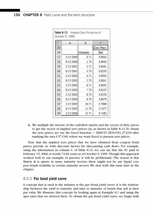
150 CHAPTER 8 Yield curve and the term structure
4. We multiply the inverse of the cash-fl ow matrix and the vector of dirty prices to get the vector of implied zero prices ( z), as shown in Table 8.13 . To obtain the zero prices, we use the Excel function � MMULT (B39:N51, J7:J19) after marking the area C57:C69, where we want Excel to present zero prices.
Note that the implied zero prices that we have obtained from coupon bond prices provide us with discount factors for discounting cash fl ows. For example, using the information in column C of Table 8.13 , we can say that the $1 paid in February 15, 2006, is worth 74.82 cents as of October 9, 1999. Though this approach worked well in our example, in practice it will be problematic. The reason is that Matrix A is sparse in many maturity sectors; there might not be any liquid cou-pon bonds available in certain maturity sectors. We deal with this issue later in the chapter.
8.2.3 Par bond yield curve
A concept that is used in the industry is the par bond yield curve. It is the relation-ship between the yield to maturity and time to maturity of bonds that sell at their par value. We illustrate this concept by looking again at Example 8.1 and using the spot rates that we derived there. To obtain the par bond yield curve, we begin with
Table 8.13 Implied Zero Prices as of October 9, 1999
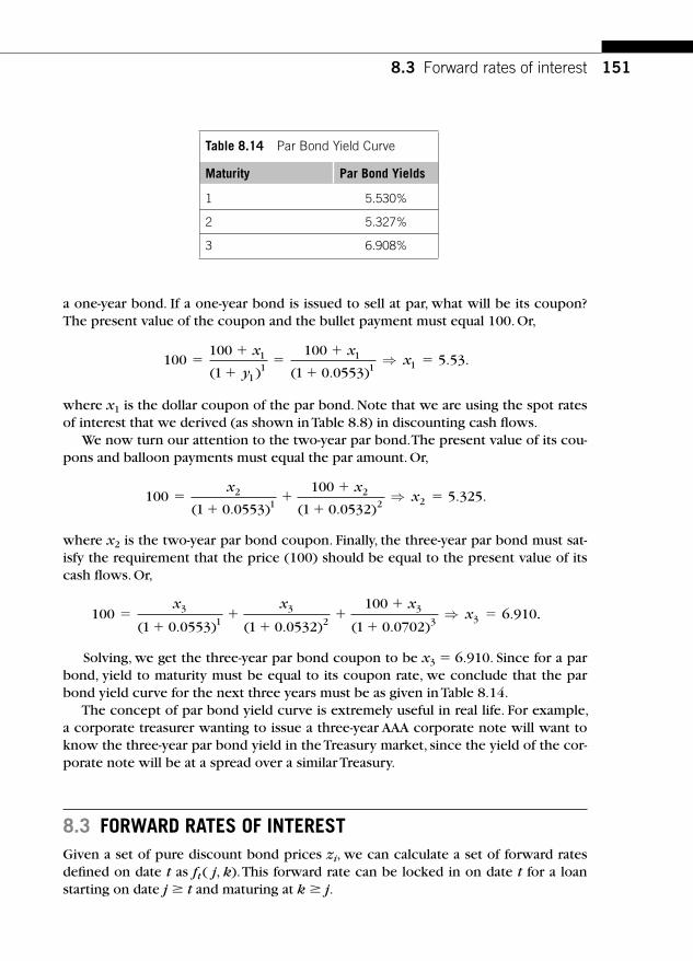
151
a one-year bond. If a one-year bond is issued to sell at par, what will be its coupon? The present value of the coupon and the bullet payment must equal 100. Or,
100100
1
100
1 0 05535 531
11
11 1�
�
��
�
��
x
y
xx
( ) ( . ). .⇒
where x 1 is the dollar coupon of the par bond. Note that we are using the spot rates of interest that we derived (as shown in Table 8.8 ) in discounting cash fl ows.
We now turn our attention to the two-year par bond. The present value of its cou-pons and balloon payments must equal the par amount. Or,
1001 0 0553
100
1 0 05325 3252
12
2 2��
��
��
x xx
( . ) ( . ). .⇒
where x 2 is the two-year par bond coupon. Finally, the three-year par bond must sat-isfy the requirement that the price (100) should be equal to the present value of its cash fl ows. Or,
1001 0 0553 1 0 0532
100
1 0 07026 9103
13
23
3 3��
��
��
��
x x xx
( . ) ( . ) ( . ).⇒ ..
Solving, we get the three-year par bond coupon to be x 3 � 6.910. Since for a par bond, yield to maturity must be equal to its coupon rate, we conclude that the par bond yield curve for the next three years must be as given in Table 8.14 .
The concept of par bond yield curve is extremely useful in real life. For example, a corporate treasurer wanting to issue a three-year AAA corporate note will want to know the three-year par bond yield in the Treasury market, since the yield of the cor-porate note will be at a spread over a similar Treasury.
8.3 FORWARD RATES OF INTEREST Given a set of pure discount bond prices zi, we can calculate a set of forward rates defi ned on date t as ft ( j, k). This forward rate can be locked in on date t for a loan starting on date j t and maturing at k j.
Table 8.14 Par Bond Yield Curve
Maturity Par Bond Yields
1 5.530%
2 5.327%
3 6.908%
8.3 Forward rates of interest

152 CHAPTER 8 Yield curve and the term structure
Formally, a forward rate between two future dates j and k, where k j is a currently agreed-upon rate at which one may borrow or lend on date j for a loan maturing on date k. How do we determine the forward rate on date t, so that we can lock the rate in for a loan that begins on date j and matures on date k (naturally, k j t )?
In Table 8.15 , we consider the strategy of investing $1 on date t at a rate of yj to get (1 � yj)
j on date j. We then sell forward these proceeds on date j at a forward rate of ft( j, k) to get (1 � yj)
j � (1 � ft ( j,k )) k � j on date k. Note that there is no risk in this transaction, since the forward rates are established on date t. (We ignore the credit risk that may arise from the nonperformance by any of the counterparties.) These are indicated in Transactions 1 and 2 in Table 8.15 . Of course, we can instead invest on date t at a rate yk to get (1 � yk ) k on date k (Transaction 3).
Note that Transactions 1 and 2 together require an investment of $1 on date t, as does Transaction 3. To prevent riskless profi ts, both strategies must produce the same cash fl ow at date k; hence, we must have
( ) ( ( , )) ( ) .1 1 1� � � � ��y f j k yjj
tk j
kk
Solving this equation, we get the forward rate:
f j, ky
yt
kk
jj
k j
( )( )
( ).�
�
��
�1
11
1⎡
⎣
⎢⎢⎢
⎤
⎦
⎥⎥⎥
Let’s now assume that j � 1 year and k � 2 years. Then,
fy
y02
2
1
1 21
11( , )
( )
( ).�
�
�� (8.9)
We illustrate the computation of a one-year forward rate in an example next.
Table 8.15 Forward Rates Determination by No-Arbitrage
Transactions on Date t Cash Flows on Date t � 0
Cash Flows on Year j
Cash Flows on Year k
1. Invest $1 at the j -year spot rate �1 (1 � yj ) j —
2. Sell forward the proceeds on date j from transaction 1 at a forward rate until date k
— — (1 � yj)j � (1 � ft(j, k))k � j
TOTAL �1 0 (1 � yj)j � (1 � ft(j, k))k � j
3. Invest $1 at the k -year spot rate �1 — (1 � yk ) k

153
Example 8.3 Let y 1 � 8%, y 2 � 9%, t � 0, j � 1, and k � 2. Using Equation 8.9, the forward rate at date 0 for the period starting date 1 and ending date 2 is
f02
1 21 0 091 0 08
1 10 009( , )( . )( . )
. %��
�� �
The same concept also applies to pure discount bonds as trading instruments. This is shown in Table 8.16 , where the transactions require no net cash fl ow on date t. But the transactions
produce a cash outfl ow of �zz
k
j
on date j and a cash infl ow of $1 on date k .
Table 8.16 Locking In Forward Rates by Trading in Zero Coupon Bonds
Transactions on Date t � 0 Cash Flows on Date t � 0
Cash Flows on Year j
Cash Flows on Year k
1. Go long in a zero maturing on year k � zk 0 � 1
2. Short the quantity zz
k
j
of zeroesmaturing on date j
zzzj
k
j
�
�zz
k
j
—
TOTAL 0
�zz
k
j
� 1
Note that we have effectively locked in the forward rate between date j and date k as
f j,kz
ztj
k
( ) .� � 1
Tables 8.15 and 8.16 illustrate that the current term structure contains the relevant informa-tion for the forward rates of interest. We may synthesize forward contracts from the spot term structure as shown in Table 8.16 . We have seen from the previous examples that the current term structure thus defi nes a series of forward rates. We now provide a detailed example of computing forward rates.
Example 8.4 The prices of pure discount bonds are provided in Table 8.17 for four maturities. Using this as the basic data, compute all the applicable forward rates as well as the par bond yields.
Note that the forward rates at Year 0 may be computed for the future periods 1 to 2, 1 to 3, 1 to 4, 2 to 3, 2 to 4, and 3 to 4. In effect, there are six forward rates that we can compute at Year 0.
8.3 Forward rates of interest

154 CHAPTER 8 Yield curve and the term structure
The forward rate at date 0 for Period 1 to 2 may be calculated as follows: We recognize that taking $1 at date 0 and investing it in a one-period zero at 5.263% and then rolling that forward at date 1 until date 2 at the currently fi xed forward rate of f 0(1,2) must yield the same dollar amount as investing at date 0 in a two-period loan at a rate of 5.409%. This leads to the equation:
1 1 0 05263 1 1 2 1 05409 1 2 5 5602
0� � � � � �( . ) ( ( , )) . ( , ) . %.f f⇒
In a similar way, the forward rate at date 0 for period 2 to 3 may be calculated as follows: We recognize that taking $1 at date 0 and investing it in a two-period zero at 5.409% and then rolling that forward at date 2 until date 3 at the currently fi xed forward rate of f 0(2,3) must yield the same dollar amount as investing at date 0 in a three-period loan at a rate of 5.567%. This leads to the equation:
1 1 05409 1 2 3 1 05567 2 3 5 8820
30� � � � �. ( ( , )) . ( , ) . %.f f⇒
The forward rate at date 0 for period 3 to 4 may be calculated as follows: We recognize that tak-ing $1 at date 0 and investing it in a three-period zero at 5.567% and then rolling that forward at date 3 until date 4 at the currently fi xed forward rate of f 0(3,4) must yield the same dollar amount as investing at date 0 in a four-period loan at a rate of 6.070%. This leads to the equation:
1 1 05567 1 3 4 1 0607 3 4 7 5930
40� � � � �. ( ( , )) . ( , ) . %.f f⇒
Now we compute the forward rates f 0(1, 3), f 0(1, 4), and f 0(2, 4). The forward rate at date 0 for period 1 to 3 may be calculated as follows: We recognize that taking $1 at date 0 and investing it in a one-period zero at 5.263% and then rolling that forward at date 1 until date 3 at the currently fi xed forward rate of f 0(1,3) must yield the same dollar amount as investing at date 0 in a three-period loan at a rate of 5.567%. This leads to the equation:
1 1 05263 1 1 3 1 05567 1 3 5 7202 3
0� � � � �. ( ( , )) . ( , ) . %.f f⇒
The forward rate at date 0 for period 1 to 4 may be calculated as follows: We recognize that tak-ing $1 at date 0 and investing it in a one-period zero at 5.263% and then rolling that forward at date 1 until date 4 at the currently fi xed forward rate of f 0(1,4) must yield the same dollar amount as investing at date 0 in a four-period loan at a rate of 6.070%. This leads to the equation:
1 1 05263 1 1 4 1 0607 1 4 6 3403 4
0� � � � �. ( ( , )) . ( , ) . %.f f⇒
Table 8.17 Zero Prices and Spot Rates
Maturity Zero Prices Spot Rate of Interest
1 0.9500 5.263%
2 0.9000 5.409%
3 0.8500 5.567%
4 0.7900 6.070%

155
The forward rate at date 0 for period 2 to 4 may be calculated as follows: We recognize that taking $1 at date 0 and investing it in a two-period zero at 5.409% and then rolling that forward at date 2 until date 4 at the currently fi xed forward rate of f 0(2,4) must yield the same dollar amount as investing at date 0 in a four-period loan at a rate of 6.070%. This leads to the equation:
1 1 05409 1 2 4 1 0607 2 4 6 7420
2 40� � � � �. ( ( , )) . ( , ) . %.f f⇒
Generally, we can compute forward rates in this manner for various forward dates in the future. What are the problems with these concepts in practice? The fi rst diffi culty arises from the fact that there are few benchmark maturities. As noted in Chapter 3, there are only eight benchmark maturities: 3 months, 6 months, 1 year, 2 years, 3 years, 5 years, 10 years, and 30 years. This means that there are signifi cant gaps in the 5-year to 10-year maturity sectors and in the 10-year to 30-year maturity sectors. Second, the frequency of auctions is low in the 30-year sector and in the quarterly refunding maturity sectors. This means that even the on-the-run issues might not trade at or near par on dates further away from the auction date. These complications not withstanding, we will show that it is possible to develop good spot-rate curves based on limited information about the par bond yield curve. We apply the bootstrap-ping principle to real-life data next.
Our analysis, however, does illustrate that the coupon bond prices contain infor-mation about the prices of pure discount bonds or discount factors. If the prices of coupon bonds are out of alignment with those of pure discount bonds, after account-ing for liquidity and coupon effects, there will be profi table trading opportunities with-out any risk. Since there are coupon and vintage effects in these securities, we should use those coupon securities that sell close to or at par in constructing the implied zero coupon bond prices. We illustrate this idea later in the chapter. More generally, this analysis indicates that the schedule of coupon bond prices and pure discount bond prices must stay in alignment to preclude profi table trading opportunities.
8.4 STRIPS MARKETS Through the Federal Reserve book-entry system, the Treasury permits certain securi-ties to be stripped. These are called STRIPS or strips, short for Separate Trading of Registered Interest and Principal Securities. Under this program, Treasury securities may be maintained in the book-entry system operated by the Federal Reserve banks in such a way that it is possible to trade, in book-entry form, interest and principal components as direct obligations of the U.S. Treasury. The Treasury fi rst made eligible for strips the 10- and 30-year issues that were made as part of the quarterly refunding on February 15, 1985. Effective May 1, 1987, securities held in stripped form became eligible for reconstituting as well. Initially only 30-year (long) bonds and 10-year notes were eligible for stripping, but this restriction has since been removed.
It should be stressed that strips are not implied zeroes. Strips are traded secu-rities directly subject to demand and supply. Implied zeroes are estimated pure
8.4 Strips markets

156 CHAPTER 8 Yield curve and the term structure
discount functions derived from the prices of coupon-paying Treasury securities. Their prices are infl uenced by the demand supply forces in the coupon securities markets. Yet, as expected, implied zeroes provide a natural benchmark for assessing the relative richness or cheapness of Treasury securities compared to strips.
Treasury strips are popular securities, and they are traded in OTC markets by dealers. Why would investors want to hold zero coupon securities such as strips? Several
motivating factors are at work here. We saw in Chapter 7 that the duration of Treasury coupon securities change with interest rates. As a result, investors who buy Treasury coupon securities to hedge against their liabilities (by matching the duration of assets with liabilities) may have to frequently rebalance their positions. When a 30-year zero coupon bond is purchased, its duration is always its time to maturity, irrespec-tive of interest rates. This may signifi cantly reduce the need to rebalance positions. Furthermore, note from Table 7.7 (in Chapter 7) that the maximum duration that can be achieved in the Treasury market using the current 30-year T-bond maturing on May 15, 2037, is about 16 years. There may be many institutional investors holding liabilities with a duration of 20 or more years, and for these investors, strips may be the only real-istic alternative. A 30-year strip has a duration of 30 years and may thus be preferred by investors with long-dated liabilities for hedging purposes. If there are many such inves-tors, the strong demand for such securities may drive up the prices of long-dated strips and bring down their yields. Later we present evidence supporting this idea.
Moreover, when a Treasury coupon bond is purchased, the investor is obliged to buy a bundle of cash fl ows; the 30-year T-bond maturing on May 15, 2037, is a bundle of 60 coupon payments (5.00% payable on May 15 and November 15 of every year) and a balloon payment on May 15, 2037. This exposes the investor to reinvestment risks if cash fl ows are needed to fund liabilities only at selected points in time in the future. Then the investor may be better off buying a few strips and customizing the cash fl ows to suit the profi le of liabilities.
The prices of Treasury coupon strips and principal-only strips as of July 2008 are plotted in Figures 8.9 and 8.10 , respectively.
Principal-only strips tend to be generally less liquid compared with strips made from coupons. First, there are far fewer principal-only strips. In Figure 8.9 , there were 53 strips from principal. By comparison, on the same date there were 118 strips from interest income. Second, interest-based strips are more uniformly distributed across the whole range of maturity, whereas the distribution of principal-based strips is skewed in favor of longer maturity sectors. There were 20 interest-based strips under 5 years, 20 between 5 years and 10 years, and 40 between 10 years and 20 years. The remaining were over 20 years in maturity. There were only nine princi-pal-based strips under 5 years, 10 between 5 years and 10 years, and 23 between 10 years and 20 years. The remaining were over 20 years in maturity.
To preclude riskless profi ts, the following restrictions must hold on the pure dis-count functions (such as strips), where zi is the price of a zero coupon bond matur-ing on date i:
z z z z zn n1 2 3 1 �… .
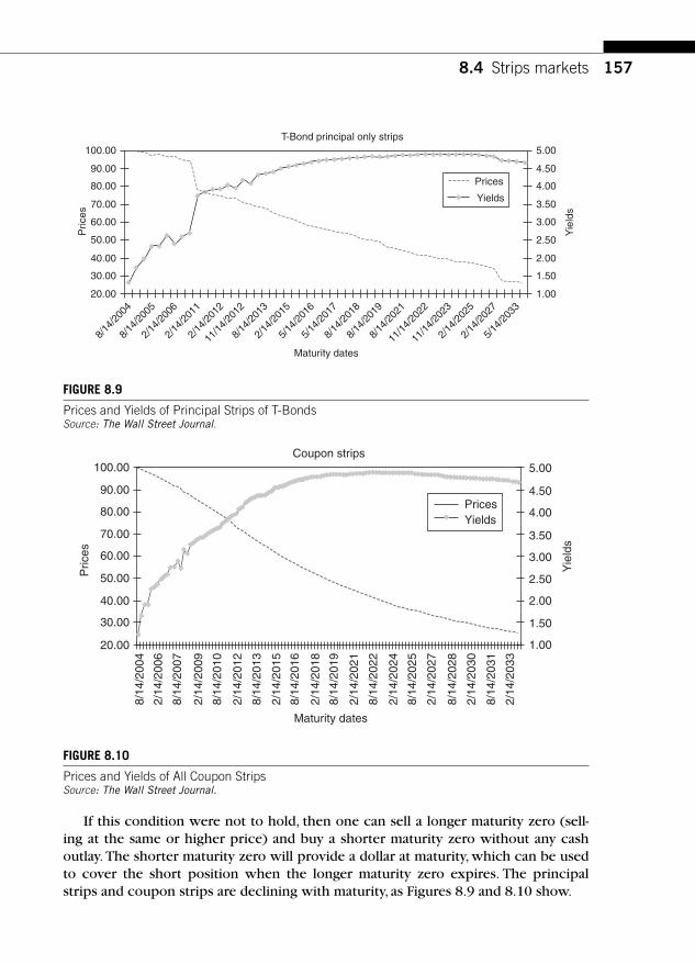
157
If this condition were not to hold, then one can sell a longer maturity zero (sell-ing at the same or higher price) and buy a shorter maturity zero without any cash outlay. The shorter maturity zero will provide a dollar at maturity, which can be used to cover the short position when the longer maturity zero expires. The principal strips and coupon strips are declining with maturity, as Figures 8.9 and 8.10 show.
100.00
90.00
80.00
70.00
60.00
50.00
40.00
30.00
20.00
8/14
/200
4
8/14
/200
7
8/14
/201
0
8/14
/201
3
8/14
/201
6
8/14
/201
9
8/14
/202
2
2/14
/200
6
2/14
/200
9
2/14
/201
2
2/14
/201
5
2/14
/201
8
2/14
/202
1
2/14
/202
4
2/14
/202
7
2/14
/203
0
8/14
/202
5
8/14
/202
8
8/14
/203
1
2/14
/203
3
5.00
4.00
3.00
4.50
3.50
2.00
2.50
1.00
1.50
Coupon strips
Maturity dates
Pric
es
Yie
lds
PricesYields
FIGURE 8.10
Prices and Yields of All Coupon Strips Source: The Wall Street Journal.
100.00
90.00
80.00
70.00
60.00
50.00
40.00
30.00
20.00
8/14
/200
4
8/14
/201
3
8/14
/200
5
2/14
/200
6
2/14
/201
1
2/14
/201
2
2/14
/201
5
2/14
/202
5
5/14
/203
3
2/14
/202
7
5/14
/201
6
5/14
/201
7
8/14
/201
8
8/14
/201
9
8/14
/202
1
11/1
4/20
22
11/1
4/20
23
11/1
4/20
12
5.00
4.00
3.00
2.00
1.50
1.00
4.50
3.50
2.50
Yie
lds
Pric
es
T-Bond principal only strips
Maturity dates
Prices
Yields
FIGURE 8.9
Prices and Yields of Principal Strips of T-Bonds Source: The Wall Street Journal .
8.4 Strips markets

158 CHAPTER 8 Yield curve and the term structure
8.5 EXTRACTING ZEROES IN PRACTICE Recall from our bootstrapping procedure that, given a set of bond coupons and maturities, it is possible for us to extract the spot rates of interest. Once we know the spot rates of interest, we can compute the relevant implied forward rates of interest. Such spot rates and implied forward rates will be contaminated by the vin-tage effects and coupon effects that we examined earlier.
Let’s consider the problem of building the spot curve without such problems. By working with newly issued bonds, which sell close to par, we can remove the vintage and coupon effects. Bonds that sell at a signifi cant premium or discount may also be subject to the tax rates of the marginal investor: A bond bought at a discount, when held to maturity, produces a capital gain that may be taxable. Such tax consid-erations may also infl uence the quoted yields, ex ante. Hence we try to work with data on bonds that sell relatively close to par. The par bond data have to be gleaned fi rst. Table 8.18 presents securities that traded close to par as of July 11, 2008.
We will use this information to fi rst determine the par bond yield curve. Once this is known, it is easy to derive spot rates and forward rates.
Since the data are sparse, we need to develop a smooth curve-fi tting procedure. A number of approaches have been used in the academic literature and in practice. We will briefl y review some of these approaches and use a nonlinear curve-fi tting scheme known as cubic spline procedure to fi t the data in Table 8.18 .
Generally, the task of extracting zero prices from the yield curve is complicated by the following factors, as pointed out earlier:
1. There are very few newly auctioned issues that sell at par at any point. In Table 8.18, we can only identify a handful of issues that sell close to par out of more than 160 issues that are outstanding in the market. We have also included a newly issued 30-year bond that is selling at a discount to par.
2. To obtain zero prices for all future maturities, we simply do not have enough information in the yield curve. We do not have many coupon bonds selling close to par maturing at every point in the future.
Table 8.18 Yields of Selected Debt Securities
Settlement Date, July 11, 2008
Issue Date Maturity Date Coupon Rate Yield Price Clean
6/30/2008 6/30/2010 2.875% 2.594% 100.03125
11/30/2007 11/30/2012 3.375% 3.322% 100.59375
6/2/2008 5/31/2013 3.500% 3.286% 100.90625
6/16/2008 5/15/2018 3.875% 3.940% 99.43750
2/15/2006 2/15/2036 4.500% 4.538% 99.37500
2/15/2008 02/15/38 4.375% 4.516% 97.62500

159
The approach to this problem is to start by specifying a simple function that describes the par bond yield function. For example, we may specify the par bond yields, denoted by yj for different maturity periods j , as follows:
y F j xj � ( , )
where x is a vector of parameters that are to be estimated. The cubic polynomial assumes that the function is a polynomial in maturity, as shown here:
YTM a b c d
i
i i i i i i( ) ( ) ( ) ( )
, ,
τ τ τ τ τ τ τ� � � � � � �
�
13 2
1 2 ….
In each benchmark maturity range, the polynomial function specifi ed previously will be chosen to fi t the yield curve. For example, when 2 τ 5, the polynomial may take a shape that best fi ts that maturity range, and so on.
Furthermore, the function and its fi rst and its second derivatives are also continu-ous within each specifi ed yield point (shown in Table 8.18 ) that we are fi tting. Using standard algorithms, we can fi t the cubic polynomial to the data. For details, we refer the reader to sources cited at the end of the chapter. We fi rst show the fi tted curve to the data in Table 8.18 and in Figure 8.11 .
0.05
0.045
0.04
0.035
0.03
0.0250 5 10 15 20 25 30
Cubic spline fitted to selected Treasury yields as of July 11, 2008
Time to maturity in years
YT
M
FIGURE 8.11
Cubic Spline Fitted Yields from Table 8.18 on July 11, 2008
8.5 Extracting zeroes in practice

160 CHAPTER 8 Yield curve and the term structure
Figure 8.11 shows the estimated par bond yields for all maturities ranging from 1 year to 30 years. Since par bond yields are equal to par bond coupons, we can use the technique of matrix inversion to determine implied zero prices. As before, we can postulate that, under ideal conditions, the par bond prices are portfolios of zero coupon bond prices. For bond i that pays a dollar coupon of Ci at date j, we can write the market price as follows:
100 1001
� ��
C z zi j Tj
T
i
i
∑
where bond i matures at date Ti. The implied zeroes and the spot curve are then extracted in a manner similar to
the procedures illustrated earlier. The resulting prices of implied zeroes are provided in Table 8.19 .
To get an idea of how well they describe reality, Figure 8.12 presents the differ-ences between the estimated implied zero prices and the market prices of coupon-only strips.
We are using the prices of implied zeroes as a benchmark for the strips mar-ket. If the implied zero prices and the strips prices are out of line, there may be a lack of alignment between the coupon bond prices and the strips prices that can be exploited for profi ts. Note that in deciding whether to strip certain strippable Treasury securities, dealers must compare the price of the strippable security to the sum of the prices of each strip that will be obtained from that coupon security. Thus, if a 30-year bond is strippable, dealers will compare the price of the 30-year bond with the sum of the prices of the 61 strips that they will get by stripping. Note that there are 60 (semiannual) coupon payments and one principal payment, equaling 61 strips. It is possible that the dealer will sell some of the strips at a price below the implied zeroes of identical maturities. The dealer will sell other strips at a price higher than the implied zeroes of identical maturities. The overall profi tability of stripping is evaluated by the expression (where Pi is the price of a strip maturing at date i and Pbond is the price of the bond which has been stripped):
π � ��
P Pi bondi 1
61
∑
If π is positive, there is a potential for profi ts from stripping. Note that the dealer should use those strip prices at which he or she can actually sell all the strips in computing the profi ts π. If π � 0, there is a potential for profi ts by reconstituting the bond; the dealer will buy all the strips and put the 30-year bond back together.
It is clear from our example based on the prices of coupon bonds and strips as of July 11, 2008, that the Treasury coupon security prices contain a great deal of information about the prices of strips. The implied zero prices and the strip prices are generally very closely aligned to each other. At intermediate maturities, the implied zero prices

161
Table 8.19 Implied Zero Prices and Market Prices of Strips
Maturity in Years Implied Zero Prices Maturity in Years Market Prices of Strips
1 0.9885 1.10 0.9764
2 0.9492 2.10 0.9489
3 0.9079 3.10 0.9155
4 0.8755 4.10 0.8761
5 0.8500 5.10 0.8416
6 0.8222 6.10 0.8044
7 0.7895 7.10 0.7635
8 0.7521 8.10 0.7200
9 0.7116 9.10 0.6765
10 0.6700 10.10 0.6411
11 0.6298 11.10 0.6048
12 0.5916 12.10 0.5704
13 0.5558 13.10 0.5399
14 0.5226 14.10 0.5120
15 0.4922 15.10 0.4857
16 0.4645 16.11 0.4631
17 0.4395 17.11 0.4392
18 0.4171 18.11 0.4168
19 0.3971 19.11 0.3977
20 0.3793 20.11 0.3790
21 0.3636 21.11 0.3611
22 0.3495 22.11 0.3472
23 0.3369 23.11 0.3315
24 0.3255 24.11 0.3196
25 0.3149 25.11 0.3057
26 0.3048 26.11 0.2929
27 0.2949 27.11 0.2803
28 0.2849 28.12 0.2697
29 0.2744 29.12 0.2599
8.5 Extracting zeroes in practice

162 CHAPTER 8 Yield curve and the term structure
are above the prices of strips. At the long end, however, strip prices are above the implied zero prices.
We can also compare the fi tted yield curve to the actual yield curve that we pre-sented at the very outset of this chapter. Such a comparison is shown in Figure 8.13 .The relevant maturity range over which we can compare is between 2 years and 30 years. Note that the fi tted curve is slightly above the actual yields between 2 years and 5 years and slightly below the actual yields in the maturity range 5 years to 10 years. The fi tted curve and actual yields correspond reasonably closely to each other in the long end of the yield curve.
We have illustrated the extraction of spot rates of interest from the par bond yield curve using a specifi c statistical (curve-fi tting) approach. There have been many approaches presented in the academic literature for fi tting a yield curve. In Nelson and Siegel (1987), it is suggested that the discount bond prices are a nonlinear function of time to maturity T � t as shown by
zrT tt
T t
�
�
��
1
1
⎛
⎝⎜⎜⎜⎜
⎞
⎠⎟⎟⎟⎟
and
re
et
T tT t
� � ��
�
��
�
θ θ θλ
θλ
λ0 1 2 2
1( )
The parameters θ 0, θ 1 , θ 2, and λ will have to be estimated to get the pure discount
factors. A simple curve-fi tting approach of the sort presented here has been used by McCulloch (1975) and Litzenberger and Rolfo (1984) . It should be emphasized that all these methods are curve-fi tting procedures; as such, they are statistical in their
0.0400
0.0300
0.0200
0.0100
0.00 5.00 10.00 15.00 20.00 25.00 30.00 35.000.0000
�0.0100
�0.0200Maturity in years
Implied zero prices minus strip prices
FIGURE 8.12
Differences Between Market Prices of Strips and Estimated Prices of Implied Zeroes

163
approach and generally do not have a sound economic foundation. Development of arbitrage-free models of term structure allows us to estimate zero prices on a more sound theoretical footing. Such models form the core of the next chapter.
SUGGESTED REFERENCES AND READINGS Balduzzi, P. , Elton, E. J. , & Green , T. C. ( 2001, December ) . Economic news and bond prices: Evidence
from the U.S. treasury market . Journal of Financial and Quantitative Analysis , 36 ( 4 ) , 523– 543 .
Johannes , M. ( 2004 ) . The economic and statistical role of jumps to interest rates . Journal of Finance , 59 , 227 – 260 .
Litterman , R. , & Scheinkman , J. ( 1991, June ) . Common factors affecting bond returns . Journal of Fixed Income , 1(1) , 54 – 61 .
Litzenberger , R. H., & Rolfo , J. ( 1984 ) . An international study of tax effects on government bonds . Journal of Finance , 39 , 1 – 22 .
MATLAB documentation on Cubic Splines.
McCulloch , J. H. ( 1975 ) . The tax-adjusted yield curve . Journal of Finance , 30 , 811 – 830 .
Warga , A. ( 1992 ) . Bond returns, liquidity, and missing data . Journal of Financial and Quantitative Analysis , 27 ( 4) , 605 – 617 .
Fitting yields using par bonds
Time to maturity in years
0.01
0.015
0.025
0.035
0.045
0.05
0.04
0.03
0.02
0 10 15 20 25 305
Fitt
ed a
nd a
ctua
l yie
lds
Cubic spline fitted yield curve and actual yield curve
FIGURE 8.13
Fitted Yields Versus Actual Yields
Suggested references and readings

This page intentionally left blank

165
CHAPTER
Fixed Income Markets and Their DerivativesCopyright 2009 by Academic Press. Inc. All rights of reproduction in any form reserved.
CHAPTER SUMMARY This chapter summarizes the important developments in arbitrage-free pricing of securities. We focus exclusively on one-factor models of term structure and how they can be used to value fi xed-income securities and their derivatives. We address the following models: random walk model of interest rates and mean-reverting inter-est rates, including the Cox, Ingersoll, and Ross model and the Vasicek model. We develop in detail the Black, Derman, and Toy model and show how it can be cali-brated to market data on yields and volatilities. We briefl y summarize many one-factor models and describe their differences. Finally, we illustrate the pricing of interest rate derivatives, including options on constant maturity yields and yield curve swaps.
9.1 INTRODUCTION In modeling term structure of interest rates, we must keep in mind the following properties of interest rates: First, short-term interest rates are more volatile than long-term interest rates. Second, short-interest rates generally exhibit some mean reversion. Third, models that we use must ensure that there are no opportunities for arbitrage. Many models have been developed for valuing the term structure. We will begin with a simple model in which rates are assumed to be lognormally distributed and price bonds so that there are no arbitrage opportunities. This model was fi rst proposed by Rendelman and Bartter (1980).
Models of yield curve have been developed to value debt securities and their deriv-atives. These models begin by specifying a process by which interest rates of certain maturities evolve over time. Then, by applying the principle of no arbitrage, all other bond prices are determined. We begin with a simple model of bond prices in which we assume that the one-year interest rates follow a simple, multiplicative random walk. Such a process is illustrated in Figure 9.1 for four points in time: t � 0, 1, 2, and 3.
Models of yield curve and the term structure 9

166 CHAPTER 9 Models of yield curve and the term structure
Note that in each year interest rates can either go up or go down with some probability. For example, at date 0, the one-year interest rate is r. It can go up to ru or go down to rd in date 1, which corresponds to the next year. From each node, interest rates can go either up or go down as shown in Figure 9.1 . The notation adopts the following conven-tion: The subscript denotes the nature of and number of moves that have taken place in the interest rates. We will assume throughout that the probability of an up move is q and that of a down move is 1 � q, irrespective of the level of the spot rate of interest. This assumption rules out the possibility that at higher interest rates in the lattice, the probability of an up move is lower than the probability of a down move, and vice versa.
More satisfactory processes, which allow for this possibility and therefore for mean reversion in interest rates, will be taken up later. This process is based on the discrete-time model of Rendelman and Bartter (1980). Consider a pure discount bond paying a dollar at date t � 3, as shown in Figure 9.2 . The notation is as follows: The subscript denotes the nature of and number of moves that have taken place in the interest rates. The fi rst argument refl ects the date that we are in, and the second argument represents the maturity date.
Note that the zero coupon bond price converges to the par value of 1 at all nodes at date t � 3. At each node we can compute the expected return over one year, and it should be the same as the one-year rate prevailing at that node. Therefore, at date t � 2, the following conditions hold:
zruuuu
( , )( , )
,2 31
1 2 3�
�
t � 0 t � 1 t � 2
rdd (2, 3)
rd (1, 2)
r � r (0, 1)
ru (1, 2)
rud (2, 3)
ruu (2, 3)
ruuu (3, 4)
ruud (3, 4)
rudd (3, 4)
rddd (3, 4)
t � 3
FIGURE 9.1
Evolution of One-Year Interest Rates

167
zruddu
( , )( , )
,2 31
1 2 3�
�
and
zrdddd
( , )( , )
.2 31
1 2 3�
�
These conditions say that the return at date t � 2 from holding a one-period bond should be equal to the one-period rate at that node. We now proceed in a recursive fashion to date t � 1. We can compute the expected return at each node at date t � 1 as follows:
1 1 22 3 1 2 3
1 3� �
� �r
qz q z
zuuu ud
u
( , )( , ) ( ) ( , )
( , ),
and
1 1 22 3 1 2 3
1 3� �
� �r
qz q z
zdud dd
d
( , )( , ) ( ) ( , )
( , ).
We can solve the two preceding equations for the bond prices on date t � 1. Proceeding this way, we can determine the bond price at date t � 0.
11 3 1 1 3
0 3� �
� �r
qz q z
zu d( , ) ( ) ( , )
( , )
9.1 Introduction
t � 0 t � 1 t � 2
zdd (2, 3)
zd (1, 3)
z (0, 3)
zu (1, 3)
zud (2, 3)
zuu (2, 3)
1
1
1
1
t � 3
FIGURE 9.2
Evolution of Three-Year Zero Prices

168 CHAPTER 9 Models of yield curve and the term structure
Note that we could expand the procedure to any arbitrary future date and com-pute the pure discount bond prices at date 0 for any maturity as the sequence z(0, 1), z(0, 2), z(0, 3), z(0, 4), … z(0, n). In addition, at each future date s in the spot rate tree, we can obtain the entire distribution of the yield curve. The ability to get the entire distribution of zero coupon bond prices is important in the valuation of interest rate derivatives. We illustrate these ideas in Example 9.1.
Example 9.1 Given the current one-year rate is 10%, the up move factor u � 1.25, the down move factor d � 0.80, the probability of an up move is q � 0.5, and the evolution of the one-year rates is given in Figure 9.3 .
19.531%
12.500%12.50%
8.00% 8.00%
5.120%
6.400%
10.00%10.0%
15.625%
t � 0 t � 1 t � 2 t � 3
FIGURE 9.3
Evolution of One-Year Interest Rates
Determine the term structure of interest rates at date t � 0 for maturities T � 1, 2, 3, and 4. We begin by solving for the price of a single-period bond. This bond pays $1 at date t � 1,
no matter which state occurs. Therefore, its price at date t � 0 is z(0, 1) � 1/1.10 � 0.9091. This is shown as
t � 0 t � 1
1
1
11.10z (0, 1) �
The yield of a one-year bond at date t � 0 is 10%. We now determine the value of a two-year bond. At date t � 1, in the up node, the value
of the bond is zu ( , ) . .1 2 1 1250 0 8889 1/� � . At date t � 1, in the down node, the value of

1699.1 Introduction
0.8249
0.8889
0.9259
1
1
1
t � 0 t � 1 t � 2
FIGURE 9.4
Evolution of Two-Year Zero Prices
the bond is zd ( , ) .1 2 0 9259 1/1.080� � . Now that we have the prices of the bond at date t � 1, we can move back to date t � 0. At date t � 0, the expected value of the bond is 0.5 � 0.8889 � 0.5 � 0.9259. The discounted value of this expected price is
z ( , ). . . .
.. .0 2
0 5 0 8889 0 5 0 92501 10
0 8249�� � �
�
The yield to maturity of the two-period bond is computed as
0 82491
110 10
22 2.
( ). %.�
��
yy⇒
The evolution of the two-year bond is given in Figure 9.4 .
We now proceed to value the three-year bond. At date t � 2, at the top node, the value of the bond is zuu ( , ) .2 3 0 8649 1/1.15625� � . At date t � 2, at the intermediate node, the value of the bond is zuu ( , ) .2 3 0 9091 1/1.10� � . At date t � 2, at the lowest node, the value of the bond is zuu ( , ) .2 3 0 9398 1/1.064� � .
Having determined the bond prices at date t � 2, we step back to date t � 1. At the top node in date t � 1, the value of the bond is the expected value of the bond in date t � 2, dis-counted by the one-period rate at the top node in date t � 1. This is given by
zu ( , ). . . .
.. .1 3
0 5 0 8649 0 5 0 90911 125
0 7884�� � �
�
In a similar way, we can determine the price of the bond at date t � 1, at the lower node as
zd ( , ). . . .
.. .1 3
0 5 0 9091 0 5 0 93981 08
0 8560�� � �
�

170 CHAPTER 9 Models of yield curve and the term structure
We now step back to date t � 0 and determine the value of the three-period bond as
z ( , ). . . .
.. .0 3
0 5 0 7884 0 5 0 85601 10
0 7475�� � �
�
The yield to maturity of the three-period bond is computed as
0 74751
110 19
33 3.
( ). %.�
��
yy⇒
The evolution of three-year bond prices is shown in Figure 9.5 .
0.7475
0.7884
0.8560
0.9398
0.9091
0.8649
t � 0 t � 1 t � 2 t � 3
1
1
1
1
FIGURE 9.5
Evolution of Three-Year Zero Prices
In a similar manner, we can determine the pricing of the four-period bond. The evolution of the four-period bond prices is shown in Figure 9.6 .
The yield to maturity of the four-period bond is computed as
0 67661
110 26
44 4.
( ). %.�
��
yy⇒
The term structure of interest rates that we have calculated is recorded in Table 9.1 . In addition to determining the term structure, we also have information on the future yield
distributions. For example, we can answer the following question: What is the distribution of two-period yields on date t � 1 (one year from now)? To address this question, we need to determine zu (1, 3) and zd (1, 3). Note that we already have this information from our analysis

171
of the three-year bond pricing. We have determined that zu (1, 3) � 0.7884 and zd (1, 3) � 0.8560. The two-year yields at date t � 1 can be determined as follows:
0 78841
112 623
22 2.
( ). %.�
��
yy
uu⇒
In a similar way,
0 85601
18 084
22 2.
( ). %.�
��
yy
dd⇒
We can determine the continuous-time limit of this binomial process for interest rates that we have used in this example. It turns out to be the lognormal process. The terminal distribution of the interest rate for any time T is lognormal. Though our model ensures that the bond prices converge to par at maturity, this process is still unsatisfactory because it assumes a lognormal
9.1 Introduction
0.6766
0.6983
0.7903
0.8822
0.8249
0.7462
t � 0 t � 1 t � 2 t � 3
0.9513
0.9259
0.8889
0.8366
FIGURE 9.6
Evolution of Four-Year Zero Prices
Table 9.1 Term Structure of Interest Rates
Bond Maturity in Years Bond Prices Yield to Maturity
1 0.9091 10.00%
2 0.8249 10.10%
3 0.7475 10.19%
4 0.6766 10.26%

172 CHAPTER 9 Models of yield curve and the term structure
distribution at any future date T. This distribution means that some extremely high interest rates can occur in the future. Note that the probability of an up move or a down move is inde-pendent of the level of the interest rates. Empirically, interest rates appear to revert to a mean level (possibly a varying mean) of interest rates. This underscores the need to examine alterna-tive processes for interest rates.
We illustrate a mean-reverting interest rate process next. In this process, the interest rate is pulled toward a central value but propagates randomly around the central value.
9.2 MODELING MEAN-REVERTING INTEREST RATES We present a simple discrete-time process in which the probability of an up move and a down move depends on the level of the interest rates. Let’s assume that the short rate follows a stochastic process specifi ed in Figure 9.7 .
Upper limit � 2μ
Lower limit, r � 0
The probabilities associated with each node are dependent on the interest rate at these nodes. These are specifi ed as
q rr
tt( ) ,� �1
2μ
and, consequently,
12
� �q rr
tt( ) .μ
rt
r ut �1 � rt � δ
r dtt �1 � rt � δ
t �2 � rt � 2δruu
t �2 � rt � 2δrud
t �2 � rtrud
t � 0 t � 1 t � 2
FIGURE 9.7
Mean-Reverting Interest Rates

173
When the interest rates reach the upper limit, the probability of a down move is 1. Similarly, when the interest rates reach the lower limit, the probability of an up move is 1. The process has lower and upper limits at 0 and 2 μ, respectively. The rates must evolve within these barriers. In the process specifi ed previously, δ rep-resents the amount by which the short rate can go up or go down in the interval (t, t � 1). This time interval could be a day, a week, or several weeks. Depending on how the time intervals are divided, the choice of the parameter δ will vary. The process specifi ed affords some fl exibility. By suitably choosing the parameter μ, both increasing and decreasing interest rate scenarios can be modeled in an expecta-tions context. When rt � μ, the probability of an up move is exactly equal to the probability of a down move. On the other hand, when rt � μ, the probability of an up move is greater than the probability of a down move, indicating that rates are expected to go up. In a similar manner, when rt � μ, the probability of an up move is less than the probability of a down move, indicating that rates are expected to go down.
Viewed in this context, we can regard the parameter μ to be the long-run mean rate of interest. The location of the current value of the short rate relative to the long-run mean is, therefore, of interest in the bond-pricing problem. Another fea-ture of interest is the speed with which the short rates are expected to approach the long-run mean value. The parameter δ can be interpreted as the speed of adjust-ment. When δ is large, the short rate rt rapidly approaches the long-run mean interest rate. On the other hand, if δ is small, the short rate approaches the long-run mean rate sluggishly. The choice of δ, μ, and the current rate rt provide fl ex-ibility in modeling various term-structure scenarios. The interest rate process we have chosen has a steady-state distribution. It can be shown that the mean and the variance of the process (as the number n of movements in the rates approaches infi nity) are given by μ and δμ/2 , respectively. Therefore, by estimating the mean and variance of the interest rate process using real-life data on interest rates, it is possible to identify the parameters δ and μ, which in turn may be used to gener-ate the interest rate tree. Example 9.2 provides a simple example to illustrate this model.
Example 9.2 Given that the current interest rate (one period) is 10%, the parameter δ � 1%, and μ � 12%, determine the term structure of interest rates at date t � 0. The evolution of the one-period interest rates is shown in Figure 9.8 .
Unlike the binomial process, here the probabilities change at each node of the lattice; hence we need to keep track of the probabilities. The next lattice, in Figure 9.9 , shows the evolution of up-move probabilities through time.
Note that the probability is exactly 0.5 when the interest rate is equal to 12%, which is the long-run mean. If the rates are below 12%, the probability of an up move increases beyond 0.5; otherwise, it decreases below 0.5.
9.2 Modeling mean-reverting interest rates

174 CHAPTER 9 Models of yield curve and the term structure
13%
11%11%
9% 9%
7%
8%
10%10%
12%
t � 0 t � 1 t � 2 t � 3
FIGURE 9.8
One-Year Interest Rate Probability Evolution
0.583
0.542
0.625
0.667
0.583
0.500
t � 0 t � 1 t � 2 t � 3
0.708
0.625
0.542
0.458
FIGURE 9.9
Mean-Reverting Probability Evolution
As we did in the case of the binomial process, we begin by solving for the price of a one-year bond. This bond pays $1 at date t � 1, no matter which state occurs. Therefore, its price at date t z� � �0 0 1 0 9091 is ( ) 1/1.10, . . The yield of one-period bond at date t � 0 is 10%.

175
We now proceed to value a two-year bond. At date t � 1, at the up node, the value of the bond is 1/1.11 � 0 9009. . At date t � 1, at the down node, the value of the bond is 1/1.09 � 0 9174. . Now that we have the prices of the bond at date t � 1, we can move back to date t � 0 and solve for the price of the two-year bond at date t � 0. At date t � 0, the expected value of the bond is (0.9009 � 0.5830 � 0.9174 � 0.4170). We discount it at 10% to get the value of a two-year bond at date t � 0.
z ( , ). . . .
.. .0 2
0 5830 0 9009 0 4170 0 91741 10
0 8253�� � �
�
The yield to maturity of the two-period bond is computed as
0 82531
110 076
22 2.
( ). %.�
��
yy⇒
The rest of the analysis is identical to that presented for the binomial process and, therefore, is not repeated here. We now move to a discussion of models that have been quite infl uential in the pricing of debt securities and their derivatives. We present two models of interest rates that display mean reversion. The fi rst one is by Vasicek and the second one by Cox, Ingersoll, and Ross. In the Vasicek model, while the interest rates display mean reversion, they can become negative. The volatility of the changes in the interest rates in the Vasicek model is a constant over a small interval of time. In contrast, in the Cox, Ingersoll, and Ross model, inter-est rates never become negative. Furthermore, the volatility of the changes in interest rates is proportional to the level of interest rates over a small interval of time.
9.2.1 The Vasicek model
The interest rate process used by Vasicek is
dr r dt dz� � �κ( ) .μ σ
The equation describes how the short-term interest rate, r, evolves through time. The right side has a deterministic component given by κ ( μ � r ) dt and a random component given by σ dz. The deterministic component goes to zero if μ � r. In this case, interest rates simply follow a random walk. The random component can take positive or negative values, and at very low interest rates this model can pro-duce negative interest rates in the future, with a positive probability.
In this process there are three parameters: μ, the long-run mean of the short-term interest rate; σ2, the variance parameter; and κ (kappa), the speed of adjustment of the short-term interest rate to the long-run mean. The Vasicek model has several intuitively appealing features. First, the short rate approaches its long-run mean with a speed determined by the parameter κ. Second, the volatility of short rates is higher than the volatility of longer maturity rates. This is consistent with the empirical evidence
9.2 Modeling mean-reverting interest rates
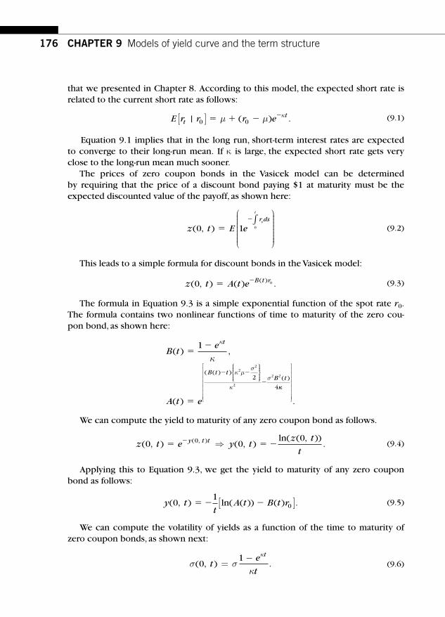
176 CHAPTER 9 Models of yield curve and the term structure
that we presented in Chapter 8. According to this model, the expected short rate is related to the current short rate as follows:
E r r r ett| ( ) .0 0[ ] � � � �μ μ κ (9.1)
Equation 9.1 implies that in the long run, short-term interest rates are expected to converge to their long-run mean. If κ is large, the expected short rate gets very close to the long-run mean much sooner.
The prices of zero coupon bonds in the Vasicek model can be determined by requiring that the price of a discount bond paying $1 at maturity must be the expected discounted value of the payoff, as shown here:
z t E er dss
t
( , )0 1 0��∫
⎛
⎝
⎜⎜⎜⎜⎜⎜⎜
⎞
⎠
⎟⎟⎟⎟⎟⎟⎟⎟ (9.2)
This leads to a simple formula for discount bonds in the Vasicek model:
z t A t e B t r( , ) ( ) .( )0 0� � (9.3)
The formula in Equation 9.3 is a simple exponential function of the spot rate r 0 . The formula contains two nonlinear functions of time to maturity of the zero cou-pon bond, as shown here:
B te
A t e
t
B t tB t
( ) ,
( )
( ( ) )( )
��
�
� �
�
1
22
2
2 22
4
κ
κ μσ
κσ
κ⎧⎨⎪⎪⎩⎪⎪
⎫⎬⎪⎪⎭⎪⎪
κκ
⎡
⎣
⎢⎢⎢⎢⎢⎢⎢
⎤
⎦
⎥⎥⎥⎥⎥⎥⎥ .
We can compute the yield to maturity of any zero coupon bond as follows.
z t e y tz t
ty t t( , ) ( , )
ln( ( , )).( , )0 0
00� � �� ⇒ (9.4)
Applying this to Equation 9.3, we get the yield to maturity of any zero coupon bond as follows:
y tt
A t B t r( , ) ln( ( )) ( ) .01
0� � �[ ] (9.5)
We can compute the volatility of yields as a function of the time to maturity of zero coupon bonds, as shown next:
σ σκ
κ
( , ) .01
te
t
t
=−
(9.6)

177
Note that Equation 9.6 implies that the volatility is a decreasing function of time to maturity.
We illustrate the Vasicek model with two examples. In the fi rst, we set the long-run mean at 8%, and the current short-term interest rate is 10%. As a result, the inter-est rates are pulled lower, leading to a downward-sloping term structure, as shown in the worksheet in Figure 9.10 . The worksheet has implemented the formulas of the Vasicek model in Equations 9.3 and 9.5. The greater the value of the speed of adjustment ( κ � 0.3), the steeper will be the term structure. Figure 9.11 illustrates the resulting downward-sloping term structure.
Finally, it should be noted that the Vasicek model implies a steady-state, long-term interest rate.
9.2 Modeling mean-reverting interest rates
FIGURE 9.10
Implementing a Vasicek Model
0.0 1.0 2.0 3.0 4.0 5.0 6.0
Time to maturity
Vasicek modelLong-run mean � 8%, Current short rate � 10%
8.80%
9.00%
9.20%
9.40%
9.60%
9.80%
10.00%
Yie
ld t
o m
atur
ity
FIGURE 9.11
Downward-Sloping Term Structure in a Vasicek Model

178 CHAPTER 9 Models of yield curve and the term structure
9.2.2 The Cox, Ingersoll, and Ross Model
In a model proposed by Cox, Ingersoll, and Ross (1985; known as CIR) , interest rates follow a mean-reverting process much like the Vasicek model we presented in the previous section. However, the variance of the changes in interest rates is propor-tional to the level of the rates.
The interest rate process they use is represented in the following equation:
dr r dt rdz� � �κ μ σ( ) (9.7)
The equation describes how the short-term interest rate, r, evolves through time. The right side has a deterministic component given by κ ( μ � r ) dt and a random component given by σ dz. The deterministic component goes to zero if μ � r. In this case, interest rates simply follow a random walk. The random component can take positive or negative values. Unlike the Vasicek model, at very low interest rates the random component matters less. Indeed, as r approaches zero, the deterministic component ensures that interest rates will always be nonnegative.
In this process, there are three parameters: μ, the long-run mean of the short-term interest rate; σ2, the variance parameter; and κ, the speed of adjustment of the short-term interest rate to the long-run mean. In addition, the parameter λ, which is related to the risk-averse behavior of investors, also affects the bond prices. These parameters must be estimated to implement the CIR model.
Prices of discount bonds are determined in the CIR (1985) model using the same arbitrage-free formula shown in Equation 9.2. This leads to a simple formula. Let the current time be denoted by 0; then a bond paying $1 at time t should be priced as
z t A t e B t r( , ) ( ) .( )0 0� � (9.8)
Equation 9.8 contains two nonlinear functions of time to maturity, as shown next:
A te
e
t
t( )
( )( )
( )
�� � � �
� �2
2 1
2
2
γγ κ γ λ
κ γ λ
γ
κμ⎛
⎝
⎜⎜⎜⎜⎜⎜⎜⎜
⎞
⎠
⎟⎟⎟⎟⎟⎟⎟⎟⎟
σσ
γ
γγ κ γ λ
2
2 1
2 1B t
e
e
t
t( )
( )
( )( )�
�
� � � �
⎛
⎝⎜⎜⎜⎜
⎞
⎠⎟⎟⎟⎟⎟
and
γ κ λ σ� � �( ) .2 22
This model can be used to generate different shapes of the yield curve. It is nec-essary that 2 κ μ σ2 to ensure that the interest rate is positive. In the CIR model,
when r ��
κμκ λ
, the term structure is downward sloping, and when r �� �
2κμκ γ λ
,
the term structure is upward sloping. For intermediate values of r, the term structure is humped.

179
The CIR model also has intuitively appealing properties: Short-term interest rates are mean reverting. The expected short-term interest rate is related to its long-term mean as shown here:
E r r r e etkt kt| ( )0 0 1( ) � � �� �μ
Moreover, interest rates in the CIR model are always nonnegative, which is not the case with the Vasicek model, where short-term interest rates can become nega-tive with a positive probability. We show two examples next. In the worksheetcontained in Figure 9.12 , we have implemented the CIR formula in Equation 9.8. Note that the current short rate is 5% and is well below the long-run mean rate of 10%. This produces an upward-sloping term structure, as shown in the worksheet in Figure 9.12 .
When the short rate is higher than the long-run mean rate, the term structure is downward sloping. We can change the short rate in the previous example to 15%. The resulting downward-sloping term structure is plotted in Figure 9.13 .
This is because the long-run mean rate ( μ) is 10% and the current interest rate is 15%. Hence, the current rate is pulled down toward the long-run mean. The higher the speed of adjustment of κ, the greater will be the inversion of the term structure.
Several authors have tested the CIR model, including Brown and Dybvig (1986), Gibbons and Ramaswamy (1994), and Pearson and Sun (1994). The fact that the model is driven by only one factor (short rate) means that its ability to capture the richness in the yield curve is somewhat limited. Gibbons and Ramaswamy (1994) estimated the parameters of the model as μ � 1.54%, κ � 12.43, λ � �6.08, and
9.2 Modeling mean-reverting interest rates
FIGURE 9.12
Implementing the Cox, Ingersoll, and Ross Model

180 CHAPTER 9 Models of yield curve and the term structure
σ � 0.49. They found that the CIR model that describes the behavior of real returns does a satisfactory job of explaining short-term T-bill returns. In much of the litera-ture, there is a general agreement that single-factor models need to be generalized, perhaps to include three factors: short-term interest rates, the spread between short-term and long-term interest rates (which is a proxy for the slope of the yield curve), and the volatility of interest rates. In the industry, single-factor models are used with an important modifi cation: Some free parameters are added to make the model fi t the market data. In the CIR model, we can describe the long-run mean rate m( t) as a function of time. Wang (1994) shows that by making μ ( t) a step function, the CIR model can be made to fi t the market data. We turn to this class of models next.
9.3 CALIBRATION TO MARKET DATA The models of interest rates that we have presented so far are not calibrated to mar-ket data. In other words, the parameters of the models are estimated, and using the estimated parameters, we compute zero prices. These zero prices might or might not correspond to the actual market prices of zeroes. If we believe there are liq-uid securities that are traded actively with narrow bid-offer spreads, we would like a model that prices them close to their market values. There is a class of term-structure models that fi nd the parameters from the market data much the same way implied volatilities are computed in equity options, using a process known as cali-bration . We present three such models of term structure here.
9.3.1 The Black, Derman, and Toy model
We begin our treatment of the fi rst of these, the Black, Derman, and Toy (BDT) model, with an illustrative example.
CIR modelLong-run mean � 10%, Current short rate � 15%
10.00%
10.50%
11.00%
11.50%
12.00%
12.50%
13.00%
13.50%
Time to maturity
0.0 1.0 2.0 3.0 4.0 5.0 6.0
Yie
ld to
mat
urity
FIGURE 9.13
Downward-Sloping Term Structure in the CIR Model

181
Example 9.3 Consider a problem in which we want the term structure model to be calibrated to the market data on one-period and two-period yields and to the volatilities presented in Table 9.2 .
9.3 Calibration to market data
Table 9.2 Data Derived from the Market
Maturity Zero YTM Volatility Annualized Zero Price
1 9.0% 22% 0.9174
2 9.5% 20% 0.8340
3 10.0% 18% 0.7513
4 10.5% 17% 0.6707
5 11.0% 16% 0.5935
In Table 9.2 , the last column contains the zero prices. For example, one-year zero price is computed as 1/1.09 and rounded to four decimals. In calibrated models, the pricing procedure is turned on its head; normally, term structure models begin with the spot-rate evolution tree (based on the parameter estimates) and then solve for the term structure as an outcome of applying no-arbitrage pricing condition. This is what we did in the previous section. The outcome of such an exercise will be an output such as the one shown in Table 9.2 . In the Black, Derman, and Toy model, however, the market data on yields is the input and the spot-rate tree is the output.
To construct the spot-rate tree, we work from the root of the lattice and proceed forward. Figure 9.14 presents one-year interest rates from Year 0 to Year 4.
r (0, 1)
ru (1, 2)
rd (1, 2)
rud (2, 3)
ruu (2, 3)
ruuu (3, 4)
ruud (3, 4)
rudd (3, 4)
rddd (3, 4)
rdd (2, 3)
t � 0 t � 1 t � 2 t � 3
FIGURE 9.14
Lattice of One-Year Interest Rates

182 CHAPTER 9 Models of yield curve and the term structure
9%
1
1
t � 0 t � 1 t � 2 t � 3 t � 4 t � 5
Price �1
1.09� 0.917431
Valuing a one-year zero
FIGURE 9.15
Price of One-Year Zero
Given the data provided in Table 9.2 , we can determine the prices of zeroes at date t � 0. We start with the price of a one-year zero in Figure 9.15 .
We now move forward to price a two-year zero. Here we are faced with two conditions: First, the two-year bond price produced by the model must match the market price. Second, the volatility of the changes in interest rates must be equal to 22%, as set forth in Table 9.2 . These two conditions can be specifi ed as follows:
0 834010 5
11 1 2
0 51
1 1 2
1 09.
.( , )
.( , )
.�
��
� ��r ru d (9.9)
2212
1 2
1 2% ln
( , )
( , )�
r
ru
d
⎛
⎝⎜⎜⎜⎜
⎞
⎠⎟⎟⎟⎟⎟
(9.10)
We can solve Equations 9.9 and 9.10 to recover the two one-year rates at date t � 1. The Excel worksheet in Figure 9.16 explains how to implement this procedure.
Now that we have determined the one-year interest rates one year ahead, we can populate the interest rate lattice as shown in Figure 9.17 , which shows the now determined zero prices.
We now proceed to determine the one-year interest rates at date t � 2. Note that at date t � 2, there are three possible interest rates, but we have only two pieces of information to per-form the calibration: market price of a three-year zero and the volatility. Hence the BDT model assumes that the interest rates are lognormally distributed. These conditions are enforced in the worksheet shown in Figure 9.18 .
The relevant mathematical conditions follow; they have been implemented in the worksheet shown in Figure 9.18 .

1839.3 Calibration to market data
FIGURE 9.16
Recovering Spot Interest Rates from Market Data
Price �0.5 � 0.891105 � 0.5 � 0.927039
1.09� 0.834011
11.0787
� 0.927039
11.1212
1
1
1
� 0.891105
9%
t � 0 t � 1 t � 2 t � 3 t � 4 t � 5
FIGURE 9.17
Valuation of Two-Year Zero

184 CHAPTER 9 Models of yield curve and the term structure
FIGURE 9.18
Extracting Spot Rates from Market Data
0 7513
0 51
1 1 20 5
11 1 2
1 122203
0 51
1
.
.( , )
.( , )
.
.
�
��
� ��
�
��r r ruu ud udd ddr( , )
.( , )
..
1 20 5
11 1 2
1 0787031 09
� ��
(9.11)
2012
1 3
1 3% ln
( , )
( , )�
y
yu
d
⎛
⎝⎜⎜⎜⎜
⎞
⎠⎟⎟⎟⎟⎟
(9.12)
Lognormality ensures the following:
r r rud uu dd( , ) ( , ) ( , ) .1 2 1 2 1 2 � � (9.13)

1859.3 Calibration to market data
1
1
1
1
9%
t � 0 t � 1 t � 2 t � 3 t � 4 t � 5
7.87%
12.22%
11.1076
� 0.902875
11.0747
� 0.9305
11.1550
� 0.865852
FIGURE 9.19
Valuation of a Three-Year Zero
Equations 9.11 –9.13 are solved in Figure 9.18 to derive the one-year rates in date t � 3. Figure 9.19 values a three-year zero based on the derived interest rates.
We proceed this way to get the entire tree. Once the tree is generated from selected market data, we can use the tree to value any interest rate derivative asset. The fully calibrated inter-est rate lattice is shown in Figure 9.20 . Note that in this fi gure, only one-year interest rates are shown at each node.
t � 0 t � 1 t � 2 t � 3 t � 4 t � 5
9%
7.87%
7.47% 7.62%
7.12%
9.54%
10.21%
10.76%
12.22%
15.50%
13.67%
12.79%
17.15%
18.31%
22.99%
FIGURE 9.20
One-Year Interest Rates Fully Calibrated to Market Data
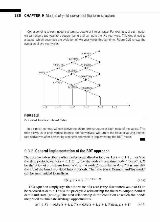
186 CHAPTER 9 Models of yield curve and the term structure
t � 0 t � 1 t � 2 t � 3 t � 4 t � 5
9.5%
8.4776%
8.1819% 7.69692%
10.6755%
11.334%
12.6471%
15.7181%
14.2998%
19.1529%
FIGURE 9.21
Calibrated Two-Year Interest Rates
Corresponding to each node is a term structure of interest rates. For example, at each node, we can price a two-year zero coupon bond and compute the two-year yield. This would lead to a lattice, which describes the evolution of two-year yields through time. Figure 9.21 shows the evolution of two-year yields.
In a similar manner, we can derive the entire term structure at each node of the lattice. This then allows us to price various interest rate derivatives. We turn to the issue of valuing interest rate derivatives after presenting a general approach to implementing the BDT model.
9.3.2 General implementation of the BDT approach
The approach described earlier can be generalized as follows: Let t � 0, 1, 2 …, let N be the time periods, and let j � 0, 1, 2 …, t be the nodes at any time node t. Let z ( t, j, T ) be the price of a discount bond at date t at node j, maturing at date T. Assume that the life of the bond is divided into n periods. Then the Black, Derman, and Toy model can be summarized formally as
z t j T e y t j T T t( , , ) .( , , )( )� � � (9.14)
This equation simply says that the value of a zero is the discounted value of $1 to be received at date T. This is the price-yield relationship for the zero coupon bond at date t and state (node) j. The next relationship is the condition at which the bonds are priced to eliminate arbitrage opportunities:
z t, j, T z t , j, T z t , j , T z t, j, t( ) { ( ) ( )} ( )� � � � � �0 5 1 0 5 1 1 1. . (9.15)

1879.3 Calibration to market data
This condition is common to all models that are used in the industry to calibrate the model to the market data. In particular, the same condition is used in the Ho and Lee (1986) model and in the Heath, Jarrow, and Morton (1992) model. The Black, Derman, and Toy (1990) model also specifi es conditions on the volatility structure,
z t , j , T) z t , j, T v t T( ( ) ( , )� � � �1 1 1 , (9.16)
where v ( t, T ) is the volatility factor for a bond with a maturity date T in period t � 1 as of date t. The volatility factor is given by
v t, T e ,t, T( ) [ ( )]� 2σ (9.17)
where σ ( t, T ) is the annualized volatility of the yield of a zero coupon bond matur-ing at date T, as evaluated at date t. As shown earlier, the model takes as market data y (0, j, T ) and σ ( 0, T ) where T � 1, 2, …, N. Note that at date t � 0 there is only one state, so j � 0. When t � 0 in Equations 9.16 and 9.17, we fi rst know the relation between z(1, 0, T ) and z(1, 1, T ) from the volatility structure. Using this in the no-arbitrage condition (Equation 9.15) yields a single nonlinear equation in z(1, 0, T )that can be solved by a univariate Newton-Raphson iterative search procedure.
To see this clearly, let us rewrite equations and for the case when t � 0. We get corresponding to Equation 9.15:
z T z T z T z( , ) [ ( , ) ( , )] ( ).0 0 0 5 1 0 0 5 1 1 0 0 1, . , . , , ,� � (9.18)
Note that in this equation, z(0, 0, T) is known for all T; hence the unknowns are z (1, 0, T ) and z (1, 1, T ). Using Equation 9.16, we get
z T z T v T( , ) ( )) .( , )1 1 1 0 0, , ,� (9.19)
In this equation, v(0, T ) is known for all T. Substituting this equation into Equation 9.18, we get
z T z T z T zv T( ) [ ( , ) ( , ) ] ( ).( , )0 0 0 5 1 0 0 5 1 0 0 0 10, , . , . , , ,� � (9.20)
This nonlinear equation can be iteratively solved for T � 1, . . . , N for z(1, 0, T ). Once we determine z (1, 0, T ), we can utilize that information to determine z (1, 1, T ).
When t 1, we have a system of two nonlinear equations that again can be solved by a bivariate Newton-Raphson search procedure. This search is a bit more compli-cated because for each T we have two nonlinear equations to solve for z(t, j, T). For each t we solve Equations (9.19) and (9.20) simultaneously. We illustrate the idea using the case when t � 1. Note that in this case, we get the following two conditions:
z j, T z j, T z j T z j( , ) [ ( , ) ( , , )] ( , , )1 0 5 2 0 5 2 1 1 2� � �. . (9.21)
and
z j T z j T v T( , , ) ( , , ) .( , )2 1 2 1� � (9.22)

188 CHAPTER 9 Models of yield curve and the term structure
For j � 0 and j � 1, the previous system can be solved for z(2, 0, T), z(2, 1, T), and z (2, 2, T ). This allows us to get the term structure at t � 2 and so on.
9.4 INTEREST RATE DERIVATIVES Interest rate derivatives range from a simple call option on yields to a complicated structure involving yield-curve swaps in which yields with different maturities are swapped between counterparties. Other interest rate derivatives include index amor-tization swaps, caps, fl oors, and delivery options in Treasury bond futures contracts. We illustrate interest rate derivatives pricing with an example of a call option on yields.
Consider the task of pricing a call option at date t � 0 on a two-period interest rate at a strike rate of k%. Assume that the option is going to expire at date t � 1. Assume that the interest rate follows a multiplicative random walk, as shown in the following lattice. The probability of an up move is q, and the probability of a down move is 1 � q.
Example 9.4 (Pricing an option on CMT yields) The market data on the yields and volatilities of yields are provided in Table 9.3 for zeroes with maturities of one to fi ve years. Construct the lattice for this market data and derive the one-year and two-year yields at each node of the lattice. Treat each period in the lattice as one year. Assume that the probability q � 1/2 . At date t � 0 a dealer wants to price a call option on two-year yields. The option will expire at date t � 2. The strike rate on this option is 9% and the notional principal of the transaction is 100 million.
Table 9.3 Market Data
Maturity Yield Volatility
1 9% 19%
2 9% 18%
3 9% 17%
4 9% 16%
5 9% 15%
We approach this problem in steps:
1. The fi rst step is to construct the calibrated lattice of one-year yields, which is shown in Figure 9.22 , based on the BDT model.
The calibration in Step 1 is done exactly as illustrated in the earlier example.

1899.4 Interest rate derivatives
13.851%
10.241%10.721%
7.332% 7.572%
5.592%
6.26445%
8.80863%9%
12.3861%
t � 0 t � 1 t � 2 t � 3
FIGURE 9.22
Lattice of One-Year Yields Calibrated to Market Data
10.645%
7.427%
6.42%
8.849%9%
12.201%
t � 0 t � 1 t � 2
FIGURE 9.23
Lattice of Two-Year Yields Calibrated to Market Data
2. The next step is to construct two-year yields at each node of the lattice, shown in Figure9.23 until Year 2.
In Step 2, we have performed the following calculations: At t � 1 in the up node, the two-year interest rate will be determined by solving for the price of a two-year zero. Let yu (1, 3) be the two-year yield at date t � 1 in the up state, where the zero matures on date t � 3. Likewise, let yd (1, 3) be the two-year yield at date t � 1 in the down state. Using these notations, we write down the volatility condition:
12
1 3
1 318ln
( , )
( , )%
y
yu
d
⎡
⎣⎢⎢
⎤
⎦⎥⎥ � (9.23)

190 CHAPTER 9 Models of yield curve and the term structure
1.4455
0
0
00.663%
3.201
t � 0 t � 1 t � 2
FIGURE 9.24
Value of the Option at Various Nodes
Equation 9.23 sets the volatility of the three-year rates (one period hence) to be equal to 18%. Also, by no arbitrage, we must have the three-year bond price be equal to the value given here:
0 51
1 1 3
1
1 1 3
1 091
1 09
2 2
3
.( ( , )) ( ( , ))
. ..
��
��
y yu d
⎡
⎣⎢⎢⎢
⎤
⎦⎥⎥⎥ (9.24)
We solve Equations 9.23 and 9.24 to get yu (1, 3) � 10.6447% and yu (1, 3) � 7.4265%. In a similar way, we can determine the yields of two-year zeroes at t � 2 as well. We determine the prices at date t � 2 for the zero maturing on date t � 4 as follows:
zr r
ruuuuu uud
uu
( , )
.( ) ( )
.( .
2 4
0 51
11
1
1
0 51
1 0 123�
��
�
��
�
⎡
⎣⎢⎢
⎤
⎦⎥⎥ 886
11 0 08808
1 0 10720 8169
) ( . ).
. .�
�
��
⎡
⎣⎢⎢
⎤
⎦⎥⎥
This implies a two-year yield of 10.644% at the top node at date t � 2. In a similar way, we can work out other two-year yields.
3. We now construct the payoffs of the call option at maturity and its values at other nodes, as shown in Figure 9.24 . At date t � 0, we show the value of the option. In Step 3, we have performed the following computations. First, we determine the payoff of the option at maturity date t � 2. At the top node, the payoffs are:
Cuu � � �max , . . . .0 12 201 9 000 3 201[ ]
At other nodes at t � 2, payoffs are zero because the strike price is higher than the two-year yields. At date t � 1, the value of the options is:
Cu �� � �
�0 5 3 201 0 5 0
1 07211 4929
. . ..
. .

1919.4 Interest rate derivatives
Obviously, Cd � 0. Working back, we determine the value of the option at the root of the lattice as:
C �� � �
�0 5 1 4929 0 5 0
1 090 6848
. . ..
. .
The value of the option is 68.48 basis points on the notional principal.
The next example illustrates how to value yield curve swaps. In a yield curve swap, one dealer (say, Dealer A) agrees to pay another dealer (say, Dealer B) con-stant maturity two-year yields. In exchange, Dealer B agrees to pay one-year constant maturity yields plus or minus a spread such that the present values of each prom-ised payment are the same. We have chosen to illustrate the swap with one-year and two-year constant maturity yields, although the swap can be done with any specifi c maturity.
Example 9.5 (Yield curve swaps) Consider a dealer who is making a market to swap one-year rates for two-year rates on a notional principal of $200 million. The swap has a tenor of two years and is reset every year. Compute the spread that should be applied to the one-year yield. Use BDT model and cali-brate it to the data shown in Table 9.4 .
Table 9.4 Market Data
Maturity Yield Volatility
1 10.0% 20%
2 11.0% 19%
3 12.0% 18%
4 12.5% 17%
5 13.0% 16%
1. We construct a lattice of one-year interest rates as shown in Figure 9.25 . 2. At each node, we now have to construct the two-year interest rates. This step is needed
since the dealer option is on two-year constant maturity interest rates. Since the option expires on date t � 2, we need to get the two-year interest rates only until this period. This is shown in Figure 9.26 .
3. Let the swap be priced such that the spread applied to the one-year rate is x. Then the swap structure may be presented as in Figure 9.27 .

192 CHAPTER 9 Models of yield curve and the term structure
21.788%
16.055%14.318%
9.792% 11.830%
8.717%
9.760%
13.767%10%
19.4182%
t � 0 t � 1 t � 2 t � 3
FIGURE 9.25
One-Year Interest Rates Lattice
15.416%
10.756%
10.001%
13.835%11%
19.135%
t � 0 t � 1 t � 2
FIGURE 9.26
Two-Year Interest Rates Lattice
t � 0 t � 1 t � 2
0
{15.416 � (14.318 � x)}
{19.135 � (19.4187 � x)}
{13.835 � (13.7669 � x)}
{10.001 � (9.760 � x)}
{10.756 � (9.7916 � x)}
FIGURE 9.27
Swap Payoffs
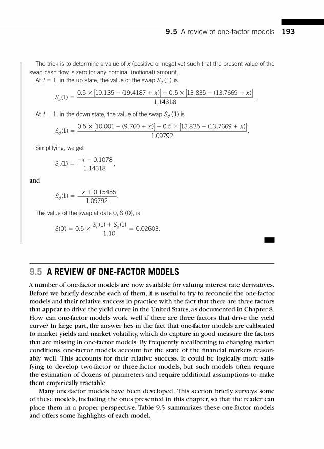
193
The trick is to determine a value of x (positive or negative) such that the present value of the swap cash fl ow is zero for any nominal (notional) amount.
At t � 1, in the up state, the value of the swap Su (1) is
Sx x
u ( ). . ( . ) . . ( . )
.1
0 5 19 135 19 4187 0 5 13 835 13 7669
1 1�
� � � � � � �[ ] [ ]44318
.
At t � 1, in the down state, the value of the swap Sd (1) is
Sx x
d ( ). . ( . ) . . ( . )
.1
0 5 10 001 9 760 0 5 13 835 13 7669
1 097�
� � � � � � �[ ] [ ]992
.
Simplifying, we get
Sx
u ( ).
.,1
0 10781 14318
�� �
and
Sx
d ( ).
..1
0 154551 09792
�� �
The value of the swap at date 0, S (0), is
SS Su d( ) .
( ) ( )
.. .0 0 5
1 1
1 100 02603� �
��
9.5 A REVIEW OF ONE-FACTOR MODELS A number of one-factor models are now available for valuing interest rate derivatives. Before we briefl y describe each of them, it is useful to try to reconcile the one-factor models and their relative success in practice with the fact that there are three factors that appear to drive the yield curve in the United States, as documented in Chapter 8. How can one-factor models work well if there are three factors that drive the yield curve? In large part, the answer lies in the fact that one-factor models are calibrated to market yields and market volatility, which do capture in good measure the factors that are missing in one-factor models. By frequently recalibrating to changing market conditions, one-factor models account for the state of the fi nancial markets reason-ably well. This accounts for their relative success. It could be logically more satis-fying to develop two-factor or three-factor models, but such models often require the estimation of dozens of parameters and require additional assumptions to make them empirically tractable.
Many one-factor models have been developed. This section briefl y surveys some of these models, including the ones presented in this chapter, so that the reader can place them in a proper perspective. Table 9.5 summarizes these one-factor models and offers some highlights of each model.
9.5 A review of one-factor models

19
4C
HA
PTE
R 9
Models of yield curve and the term
structure
Table 9.5 A Summary of Some One-Factor Models
Model Interest Rate Specifi cation Calibration Highlights
Vasicek dr � κ ( μ � r ) dt � σ dW The basic model is not calibrated to market data.
Mean reversion and a simple formula for discount bond prices and some interest rate derivatives. Allows negative interest rates.
Cox, Ingersoll, and Ross (1985)
dr r dt r dW� � �κ μ σ( ) The basic model is not
calibrated to market data. Mean reversion and a simple formula for discount bond prices and some interest rate derivatives. Interest rates are nonnegative.
Ho and Lee (1986) dr � a ( t ) dt � σ dW The basic model is calibrated to market yields.
Assumes normality of interest rates; interest rates can become negative. Allows for simple closed form solutions to zero coupon prices and some derivatives.
Black, Derman, and Toy (1990)
dr a tt
trt
dt dW� � �( )ln( )∂σσ
σ( )
( )∂
⎡
⎣⎢⎢
⎤
⎦⎥⎥
The model is calibrated to market yields and volatilities.
Combines mean reversion and volatility to keep the model tractable. Easy to implement.
Black and Karasinski (1991) d (ln r ) � [ a ( t) � b ( t )ln r ] dt � σ ( t ) dW The model is calibrated to market yields and volatilities.
Separates mean reversion and volatility.

195Suggested references and readings
Note that these models all have the property that bonds fully span all uncertainty in fi xed income markets; in other words, all interest rate derivatives can be hedged using underlying bonds of different maturities. With a single-factor model, the implication is even starker: All bonds are instantaneously perfectly correlated! Recent papers have correctly argued that the volatility risks that are present in interest rate derivatives are not hedged by bonds. A notable contribution in this respect is the paper by Collin-Dufresne and Goldstein (2002) , who provide empirical evidence that suggests that interest rate volatility risk cannot be hedged by a portfolio consisting solely of bonds. In addition, they demonstrate that interest rate derivatives are affected by volatility risk, which is not a major factor in pricing swaps or similar fi xed income securities. This criticism would suggest that stochastic volatility (which is one way of introducing vola-tility risk) or jumps in volatility may be very relevant in pricing interest rate derivatives. These important elements are missing in one-factor models that are reviewed here.
Heath, Jarrow, and Morton (1992) developed a powerful framework for modeling term structure. Many of the models discussed here can be thought of within their general framework. For details the reader is referred to their original paper cited in the references. Another framework, known as the LIBOR market model, has been developed for valuation of interest rate derivatives in which the forward rates of interest play a key role.
SUGGESTED REFERENCES AND READINGS Black , F. , Derman , E., & Toy , W. ( 1990 ) . A one-factor model of interest rates and its application to trea-
sury bond options . Financial Analysts Journal , 46 ( 1) , 33 – 39 .
Brace , A., Gatarek , D. , & Musiela , M. ( 1997 ) . The market model of interest rate dynamics . Mathematical Finance , 7 ( 2) , 127 – 155 .
Collin-Dufresne , P. , & Goldstein , R. S. ( 2002, August ) . Do bonds span the fi xed income markets? Theory and evidence for unspanned stochastic volatility . Journal of Finance , 57 ( 4) , 1685 – 1730 .
Cox , J. C. , Ingersoll , J. , & Ross , S. ( 1985 ) . A theory of the term structure of interest rates . Econometrica , 53 , 385 – 407 .
Gibbons , M. R. , & Ramaswamy , K. ( 1993 ) . The term structure of interest rates: Empirical evidence . Review of Financial Studies , 6 , 619 – 658 .
Heath , D. , Jarrow , R. , & Morton , A. ( 1992 ) . Bond pricing and the term structure of interest rates: A new methodology for contingent claims valuation . Econometrics , 60 ( 1) , 77 – 105 .
Ho, T. S. Y. , & Lee , S. ( 1986 ) .Term structure movements and pricing interest rate contingent claims . Journal of Finance , XLI ( 5) , 1011 – 1029 .
Hull , J. , & White , A. ( 1990 ) . Pricing interest-rate derivative securities . Review of Financial Studies , 3 ( 4) , 573 – 592 .
Miltersen , K., Sandmann , K. , & Sondermann , D. ( 1997, March ) . Closed form solutions for term struc-ture derivatives with lognormal interest rate . Journal of Finance , 52 ( 1) , 409 – 430 .
Rendleman , R. J. , Jr. , & Bartter , B. J. ( 1980 ) . The pricing of options on debt securities . Journal of Financial and Quantitative Analysis , XV ( 1) , 11 – 24 .
Wang , C. ( 1994 ) . Interest rate swaps . Unpublished doctoral dissertation . New York : ColumbiaBusiness School .

This page intentionally left blank
CHAPTER
197Fixed Income Markets and Their DerivativesCopyright 2009 by Academic Press. Inc. All rights of reproduction in any form reserved.
10 CHAPTER SUMMARY This chapter provides some time-series evidence on loan and bond defaults, recovery rates, and credit spreads and interprets their relationship to business cycles. We describe the ratings conventions, the migration of fi rms from one rating category to another, and the difference between investment-grade and noninvestment-grade debt. We explain structural and reduced-form models of default and illustrate their applications in valuing corporate debt securities. We explain how default probabilities can be computed using equity prices and structural models of default. The relationship between the spreads of senior and subordinated debt is derived in a structural context and interpreted. The role of costly fi nancial distress on the pricing of corporate debt is discussed. Finally, the chap-ter shows that the credit spreads are not only related to the probability of default and recovery rates but also to changes in the risk premium in the market.
10.1 DEFAULTS, BUSINESS CYCLES, AND RECOVERIES Credit risk is the possibility of default by one of the counterparties in a fi nancial trans-action. The probability of default affects the future cash fl ows of the fi nancial trans-action; for example, defaulted debt may trade at just 40% of the par value, resulting in potentially unanticipated losses. Hence the current market price (or value) of the transaction in a default-risky security (such as corporate debt) is the risk-adjusted pres-ent value of future promised cash fl ows. Rating agencies defi ne default as any missed or delayed disbursement of contractual obligations (interest, sinking funds, or princi-pal), bankruptcy, receivership, or distressed exchanges. Credit-rating agencies broadly classify debt into investment grade and noninvestment (or speculative) grade.
As shown in Table 10.1 , from 1970 through 2006 there have been defaults by both investment-grade companies and by speculative-grade companies. In some years the
Modeling credit risk and corporate debt securities

198 CHAPTER 10 Modeling credit risk and corporate debt securities
Table 10.1 Rated Global Corporate Bond and Loan Default Volumes, 1970 –2006 ($ Millions)
Cohort Investment Grade Speculative Grade All Rated
Bond Loan Total Bond Loan Total Bond Loan Total
1970 154.0 0 154 823.5 0 823.5 977.5 0 977.5
1971 0 0 0 131.8 0 131.8 131.8 0 131.8
1972 0 0 17.4 94.3 0 94.3 111.7 0 268.2
1973 17.4 0 17.4 94.3 0 94.3 111.7 0 111.7
1974 0 0 0 69.4 0 69.4 69.4 0 111.7
1975 0 0 0 273.5 0 273.5 273.5 0 273.5
1976 0 0 0 37.3 0 37.3 37.3 0 37.3
1977 68.0 0 68.0 184.6 0.0 184.6 252.6 0.0 252.6
1978 0.0 0.0 0.0 111.9 0.0 111.9 111.9 0.0 111.9
1979 0 0 0 18.4 0 18.4 18.4 0 18.4
1980 0 0 0 302.2 0 302.2 302.2 0 302.2
1981 0 0 0 47.5 0 47.5 47.5 0 47.5
1982 243.1 0 243.1 513.1 0 513.1 758.2 0 758.2
1983 0 0 0 1257.0 0 1257.0 1257.0 0 1257.0
1984 183.3 0 183.3 398.8 0 398.8 582.1 0 582.1
1985 0 0 0 1704.8 0 1704.8 1704.8 0 1704.8
1986 1782 0 178.2 3759.3 0 3759.3 3937.4 0 3937.4
1987 0 0 0 9131.7 241.5 9373.2 9131.7 241.5 9373.2
1988 0 0 0 5642.2 361.0 6003.0 5642.0 361.0 6003.0
1989 1505.9 0 1505.9 10336.0 0 10336.0 11842.0 0 11842.0
1990 0.0 0 0 20490.5 1602.8 22093.3 20490.5 1602.8 22093.3
1991 1348.0 0 1348.0 15812.8 349.6 16162.4 17160.8 349.6 17510.4
1992 0 0 0 6340.2 698.1 7038.3 6340.2 698.1 7038.3
1993 0 0 0 2633.9 423.8 3057.5 2633.9 423.8 3057.7
1994 0 0 0 2657.1 299.4 2956.5 2657.1 299.4 2956.5
1995 0 0 0 6774.5 337.3 7111.8 6774.5 337.3 7111.8
1996 0 0 0 4100.5 1435.0 5535.5 4100.5 1435.0 5535.5
1997 0 0 0 5128.7 948.0 6076.7 5128.7 948.0 6076.7
1998 399.0 0 399.0 10499.7 1811.1 12310.8 10898.7 1811.1 12709.8
(Continued)

199
volume has been rather high. For example, in 1990, following the banking crisis in the United States, dollar volume of defaults by all rated companies ballooned to $22,093 million. Nearly a decade later, in the period 1999 –2002, the volume of default again ballooned following the bursting of the dot-com bubble, reaching levels ranging from $41,812 million in 1999 to $212,029 million in 2002. Table 10.1 also makes it clear that the speculative-grade companies accounted for all the defaults in 1990. In sharp contrast, in 1999, over 60% of the volume of defaults came from investment-grade com-panies. In fact, a review of data during 1999 –2002 shows that investment-grade com-panies have contributed as much as the speculative-grade companies to the volume of defaults. This trend resulted from some defaults of companies such as Enron and WorldCom, which were companies with high reputation even a few months prior to their defaults and eventual bankruptcies.
Companies default in many ways. They can miss payments to creditors on a timely basis (delinquencies). They might fail to pay or live up to contractual obli-gations (such as paying promised coupons or making contracted sinking fund payments). They can fi le for bankruptcy protection under Chapter 11 of the bank-ruptcy code, or they could decide to liquidate their business under Chapter 7 of the bankruptcy code. Often corporate borrowers enter into workouts, and this process can lead to exchange offers in which old debt contracts are replaced by new debt contracts, which may be less valuable to the creditors. Each one of these events is an example of a credit event. These credit events have occurred in varying proportions in the United States.
These credit events are costly; they lead to costly renegotiations, debt service reductions, and potential liquidations. Often they lead to reorganizations. More often, fi rms miss their contractual obligations or settle with their creditors out of court.
Table 10.1 (Continued)
Cohort Investment Grade Speculative Grade All Rated
Bond Loan Total Bond Loan Total Bond Loan Total
1999 460.9 1225.0 1685.9 27897.3 12229.6 40126.9 28358.3 13454.6 41812.8
2000 4115.5 3950.0 8065.5 26481.1 22269.3 44750.4 30596.5 26219.3 56815.8
2001 22350.8 5363.60 27713.8 81217.0 31206.3 112423.3 103567.8 36569.3 140137.6
2002 55600.0 13121.9 68801.9 110323.6 32904.1 143227.8 166003.7 46026.0 212029.7
2003 0 0 0 34976.3 9691.4 44667.7 34976.3 9691.4 44667.7
2004 0 0 0 14790.4 3826.8 18617.2 14790.4 3826.8 18617.2
2005 2155.0 2825.0 4980.0 27232.4 8744.6 35977.0 29387.4 11569.6 40957.0
2006 0 0 0 7788.5 2629.6 10418.1 7788.5 2629.6 10418.1
Source : David T. Hamilton, Sharon Ou, Frank Kim, and Richard Cantor, “ Corporate Default and Recovery Rates, 1920 – 2006, ” Moody’s Investor Service, Global Research, February 2007.
10.1 Defaults, business cycles, and recoveries

200 CHAPTER 10 Modeling credit risk and corporate debt securities
Formal bankruptcy procedures are typically sought when negotiations fail to resolve matters.
Default may be the result of a macroeconomic factor such as recession. It can also be due to company- or industry-specifi c factors. In general, both these factors are important. They can result in lack of liquidity or insolvency, both factors that can cause default. The relation between business cycles and defaults can be better under-stood by reviewing Figure 10.1 , which documents annual default rates and corporate spreads over Treasury benchmarks during the 1920 –2007 period. The shaded areas in the panels denote recessionary periods in the United States.
Spikes in default rates during the 1930s and early 1970s, accompanied by widen-ing spreads, suggest a strong relationship between economic slowdown and corpo-rate fi nancial health.
Recession may lead to slowdowns and correlated defaults by many fi rms within the same industry. One can therefore expect the default rates to go up and the recovery
1920 1930 1940 1950 1960 1970 1980 1990 20000
2
4
6
8
Def
ault
rate
(%
)Panel A: Annual default rates
Jan20 Jun32 Nov44 Apr57 Sep69 Feb82 Jul94 Jan070
100
200
300
400
500
600
Spr
ead
(bas
is p
oint
s)
Panel B: Monthly Baa–Aaa yield spreads
FIGURE 10.1
Business Cycles, Defaults, and Credit Spreads Source : This fi gure is taken from Hui Chen, “Macroeconomic Conditions and the Puzzles of Credit Spreads and Capital Structure, ” 2008 working paper, Sloan School, MIT, Annual Global Corporate Default Rates and Monthly Baa-Aaa Credit Spreads, 1920 –2006 . Shaded areas are NBER-dated recessions. For annual data, any calendar year during which at least fi ve months are in a recession as defi ned by NBER is treated as a recession year. Data source: Moody’s.

201
rates for lenders to go down; as more companies within the same industry are more likely to default in recession, the resale values of assets may be much lower in reces-sion. In contrast, the value of assets of a company that defaults when other com-panies in the same industry are doing better could be much higher. Note in Figure 10.1 that the defaults signifi cantly increased during the Great Depression years (the 1930s). The late 1980s and early 1990s again saw an increase in the number of defaults in the economy. Marketwide factors do play a role in triggering defaults.
To give a sense of recovery rates to lenders, Table 10.2 presents the historical experience.
Debt securities that are subject to default risk can differ signifi cantly in terms of their seniority in the capital structure, the level of protection they have by way of security, and so on. Depending on their status, the expected recovery rate condi-tional on default can change.
Table 10.2 shows that the historical recovery rates of various categories of debt instruments differ signifi cantly. Notice that the bank loans and senior secured debt securities tend to recover about 70% of the par value in the event of default. By contrast, junior unsecured debt instruments have much lower recovery rates as a fraction of their par value. Generally the recovery rates were low, on average, in the 1990 –1991 period and the 2000 –2001 period. What factors affect the recovery rates? An important consideration is the relative bargaining positions of lenders and borrowers. This is, in turn, greatly infl uenced by the underlying bankruptcy code and its enforceability. For example, nonsovereign loans and bonds come under the rubric of a bankruptcy code. On the other hand, sovereign debt does not necessarily fall under a bankruptcy code. This affects lenders ’ ability to access borrowers ’ collateral in the event of default. Availability of secured collateral and its value under fi nancial distress are yet another factor that infl uences the recovery rates. The presence of multiple creditors and the existence of bank debt affect the recovery rates as well. Bank debt is senior and is typically secured. Banks closely monitor their loans. Thismonitoring is benefi cial to other creditors. On the other hand, the fact that the bank debt is secured implies that less collateral is available to other creditors in the event of default.
10.2 RATING AGENCIES Information about a borrower’s fi nancial health comes from two sources: rating agencies and market prices. Moody’s, Standard & Poor’s, Fitch, and the like produce information about the credit standing of borrowers. Often borrowers will pay money to have their debt rated. The information produced by the rating agencies changes discretely as and when the agencies update their evaluations. Much of the evidence on recovery ratios, defaults, and the like reported in this book came from Moody’s.
Rating agencies rate debt instruments into two broad categories and then clas-sify them into fi ner partitions within each of these broad categories, as shown in Table 10.3 .
10.2 Rating agencies
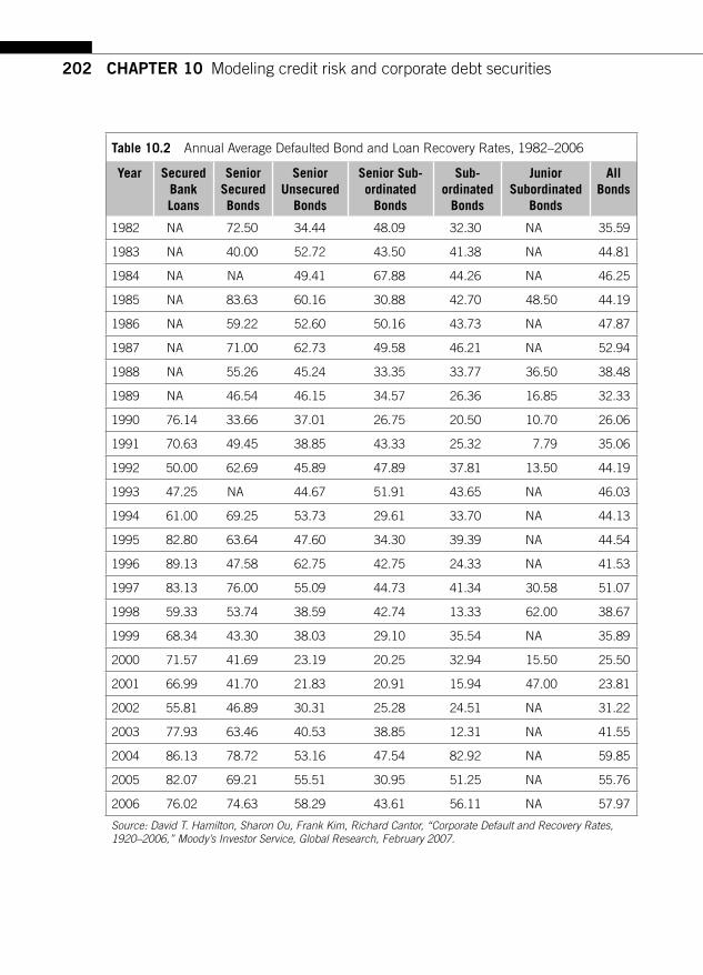
202 CHAPTER 10 Modeling credit risk and corporate debt securities
Table 10.2 Annual Average Defaulted Bond and Loan Recovery Rates, 1982 –2006
Year SecuredBankLoans
Senior SecuredBonds
Senior Unsecured
Bonds
Senior Sub-ordinated
Bonds
Sub-ordinated
Bonds
Junior Subordinated
Bonds
All Bonds
1982 NA 72.50 34.44 48.09 32.30 NA 35.59
1983 NA 40.00 52.72 43.50 41.38 NA 44.81
1984 NA NA 49.41 67.88 44.26 NA 46.25
1985 NA 83.63 60.16 30.88 42.70 48.50 44.19
1986 NA 59.22 52.60 50.16 43.73 NA 47.87
1987 NA 71.00 62.73 49.58 46.21 NA 52.94
1988 NA 55.26 45.24 33.35 33.77 36.50 38.48
1989 NA 46.54 46.15 34.57 26.36 16.85 32.33
1990 76.14 33.66 37.01 26.75 20.50 10.70 26.06
1991 70.63 49.45 38.85 43.33 25.32 7.79 35.06
1992 50.00 62.69 45.89 47.89 37.81 13.50 44.19
1993 47.25 NA 44.67 51.91 43.65 NA 46.03
1994 61.00 69.25 53.73 29.61 33.70 NA 44.13
1995 82.80 63.64 47.60 34.30 39.39 NA 44.54
1996 89.13 47.58 62.75 42.75 24.33 NA 41.53
1997 83.13 76.00 55.09 44.73 41.34 30.58 51.07
1998 59.33 53.74 38.59 42.74 13.33 62.00 38.67
1999 68.34 43.30 38.03 29.10 35.54 NA 35.89
2000 71.57 41.69 23.19 20.25 32.94 15.50 25.50
2001 66.99 41.70 21.83 20.91 15.94 47.00 23.81
2002 55.81 46.89 30.31 25.28 24.51 NA 31.22
2003 77.93 63.46 40.53 38.85 12.31 NA 41.55
2004 86.13 78.72 53.16 47.54 82.92 NA 59.85
2005 82.07 69.21 55.51 30.95 51.25 NA 55.76
2006 76.02 74.63 58.29 43.61 56.11 NA 57.97
Source : David T. Hamilton, Sharon Ou, Frank Kim, Richard Cantor, “Corporate Default and Recovery Rates, 1920–2006,” Moody’s Investor Service, Global Research, February 2007.

203
First, note that debt securities are classifi ed into “investment grade ” and “ below investment grade, ” or “junk grade. ” This is a very broad classifi cation. Note that the average default rates are predictably much lower for investment-grade debt and much higher for noninvestment-grade debt. Within each broad category are several subclassifi cations that attempt to group fi rms into a ranking of credit worthiness. Moody’s accords its highest ranking, Aaa, and Standard & Poor’s accords AAA. At the time borrowers want to enter the debt markets to raise capital, their ratings become relevant to their cost of borrowing. In addition, evidence suggests that certain actions of rating agencies have an infl uence on credit spreads. For example, when a fi rm’s debt obligations are downgraded from investment grade to noninvestment grade, there is usually a very strong market reaction. This is in large part due to the fact that institutional investors who are indexed to investment-grade indexes can no longer hold securities that have been downgraded to noninvestment grade. General Motors and Ford had that experience when their debt was downgraded from invest-ment to noninvestment grade. Sometimes a fi rm’s downgrade can trigger margin calls and collateral by counterparties.
For example, in September 2008, Moody’s cut AIG’s senior unsecured debt rat-ing to A2 from Aa3, whereas S &P reduced AIG’s long-term counterparty rating by three notches, from AA – to A –. The cuts had the potential for triggering collateral calls from the debt investors who bought insurance from AIG through credit default swaps, because the likelihood of default on the swaps had increased, and so the investors require more of a reward to hold onto them. According to a regulatory fi l-ing AIG made in August 2008, the insurer’s CDS counterparties can demand an addi-tional $14.5 billion in collateral.
Table 10.3 Credit-Rating Categories
Category Moody’s Standard & Poor’s
Grade Average Default Rate Per Year,
1970 – 1995 (%)
Grade Average Default Rate Per Year,
1981 – 1994 (%)
Investment grade Aaa Aa, Aa1, Aa2,Aa3 A, A1, A2, A3 Baa, Baa1, Baa2, Baa3
0.00 0.03 0.01 0.13
AAA AA � , AA, AA � A � , A, A � BBB � , BBB, BBB�
0.00 0.00 0.07 0.25
Below investment grade ( “ junk ” )
Ba, Ba1, Ba2, Ba3 B, B1, B2, B3 Caa, Ca, C
1.42 7.62 N/A
BB � , BB, BB � B � , B, B � CCC, CC, C
1.17 5.39 19.96
Default D D
Source: Moody’s and Standard & Poor’s.
10.2 Rating agencies
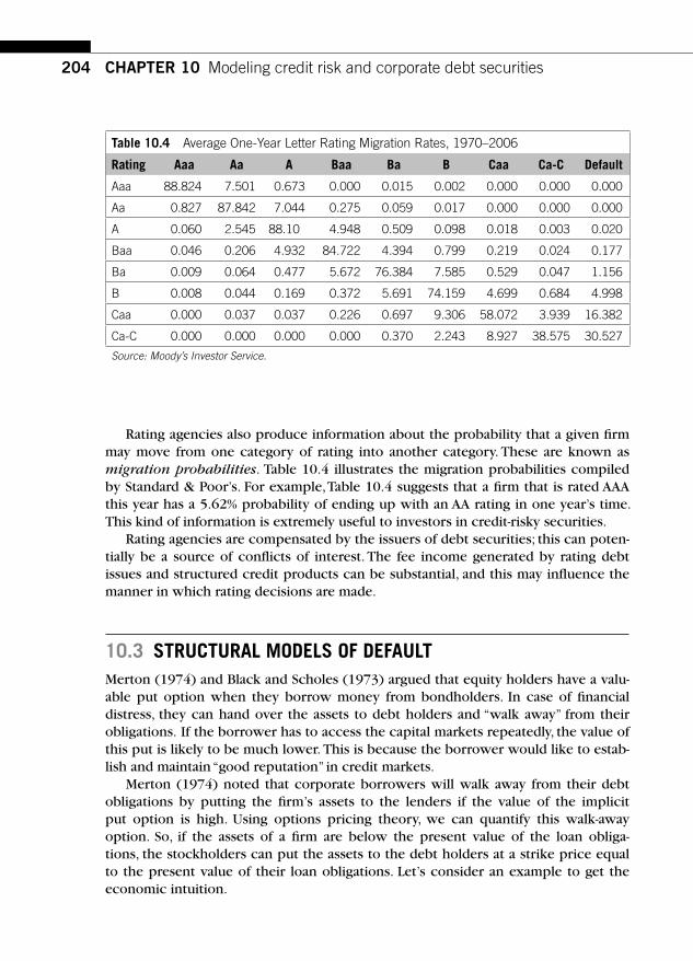
204 CHAPTER 10 Modeling credit risk and corporate debt securities
Rating agencies also produce information about the probability that a given fi rm may move from one category of rating into another category. These are known as migration probabilities. Table 10.4 illustrates the migration probabilities compiled by Standard & Poor’s. For example, Table 10.4 suggests that a fi rm that is rated AAA this year has a 5.62% probability of ending up with an AA rating in one year’s time. This kind of information is extremely useful to investors in credit-risky securities.
Rating agencies are compensated by the issuers of debt securities; this can poten-tially be a source of confl icts of interest. The fee income generated by rating debt issues and structured credit products can be substantial, and this may infl uence the manner in which rating decisions are made.
10.3 STRUCTURAL MODELS OF DEFAULT Merton (1974) and Black and Scholes (1973) argued that equity holders have a valu-able put option when they borrow money from bondholders. In case of fi nancial distress, they can hand over the assets to debt holders and “walk away ” from their obligations. If the borrower has to access the capital markets repeatedly, the value of this put is likely to be much lower. This is because the borrower would like to estab-lish and maintain “good reputation ” in credit markets.
Merton (1974) noted that corporate borrowers will walk away from their debt obligations by putting the fi rm’s assets to the lenders if the value of the implicit put option is high. Using options pricing theory, we can quantify this walk-away option. So, if the assets of a fi rm are below the present value of the loan obliga-tions, the stockholders can put the assets to the debt holders at a strike price equal to the present value of their loan obligations. Let’s consider an example to get the economic intuition.
Table 10.4 Average One-Year Letter Rating Migration Rates, 1970 –2006
Rating Aaa Aa A Baa Ba B Caa Ca-C Default
Aaa 88.824 7.501 0.673 0.000 0.015 0.002 0.000 0.000 0.000
Aa 0.827 87.842 7.044 0.275 0.059 0.017 0.000 0.000 0.000
A 0.060 2.545 88.10 4.948 0.509 0.098 0.018 0.003 0.020
Baa 0.046 0.206 4.932 84.722 4.394 0.799 0.219 0.024 0.177
Ba 0.009 0.064 0.477 5.672 76.384 7.585 0.529 0.047 1.156
B 0.008 0.044 0.169 0.372 5.691 74.159 4.699 0.684 4.998
Caa 0.000 0.037 0.037 0.226 0.697 9.306 58.072 3.939 16.382
Ca-C 0.000 0.000 0.000 0.000 0.370 2.243 8.927 38.575 30.527
Source : Moody’s Investor Service.

205
Example 10.1 Consider a fi rm that has issued a zero coupon debt with 100 face value. On the maturity date of debt, the payoffs to debt holders will look like those in Figure 10.2 .
100
100
Value of the firm
FIGURE 10.2
Value of Corporate Debt at Maturity
Note that when the fi rm is doing well, debt holders will get back the face value; on the other hand, when the fi rm is doing poorly, the most that they can hope to get is simply the value of the fi rm, ignoring dead-weight losses associated with fi nancial distress. A risk-free zero coupon bond will pay off 100 no matter what happens. So, the difference between the payoffs of a risk-free zero coupon bond and a risky zero coupon bond can be represented as shown in Figure 10.3 .
Figure 10.2 shows that corporate debt investors are essentially short a put option: When the value of the fi rm is low, equity holders can put the fi rm to bond investors and walk away from their contractual debt obligations. This approach implies the following important relationship:
Risky loan Risk-free loan Put value to default� �
or
Risk-free loan Risky loan Put option� �
The spread is the value of the put option on the assets of the borrower with a strike price equal to the promised value of debt obligations. Based on our understanding of options pricing, we can assert the following: The spread should increase with volatility. The spread should increase with leverage. The spread typically should increase with time to maturity.
Option pricing models can now be applied to value corporate debt securities. In the pricing of corporate debt securities, options-pricing insights have been used extensively. The design of corporate debt contracts, as well as their valuation, must account for the fact that the managers have the option of walking away from the
10.3 Structural models of default
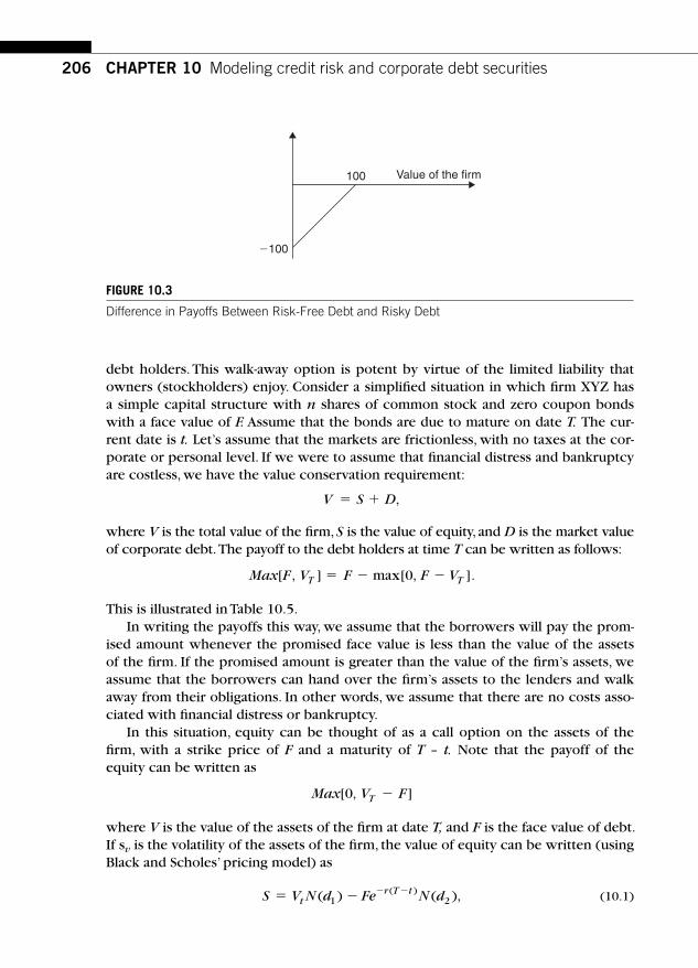
206 CHAPTER 10 Modeling credit risk and corporate debt securities
100 Value of the firm
�100
FIGURE 10.3
Difference in Payoffs Between Risk-Free Debt and Risky Debt
debt holders. This walk-away option is potent by virtue of the limited liability that owners (stockholders) enjoy. Consider a simplifi ed situation in which fi rm XYZ has a simple capital structure with n shares of common stock and zero coupon bonds with a face value of F. Assume that the bonds are due to mature on date T. The cur-rent date is t. Let’s assume that the markets are frictionless, with no taxes at the cor-porate or personal level. If we were to assume that fi nancial distress and bankruptcy are costless, we have the value conservation requirement:
V S D� � ,
where V is the total value of the fi rm, S is the value of equity, and D is the market value of corporate debt. The payoff to the debt holders at time T can be written as follows:
Max F V F F VT T[ , ] max[ , ].� � �0
This is illustrated in Table 10.5 . In writing the payoffs this way, we assume that the borrowers will pay the prom-
ised amount whenever the promised face value is less than the value of the assets of the fi rm. If the promised amount is greater than the value of the fi rm’s assets, we assume that the borrowers can hand over the fi rm’s assets to the lenders and walk away from their obligations. In other words, we assume that there are no costs asso-ciated with fi nancial distress or bankruptcy.
In this situation, equity can be thought of as a call option on the assets of the fi rm, with a strike price of F and a maturity of T – t. Note that the payoff of the equity can be written as
Max V FT[ , ]0 �
where V is the value of the assets of the fi rm at date T, and F is the face value of debt. If s v is the volatility of the assets of the fi rm, the value of equity can be written (using Black and Scholes ’ pricing model) as
S V N d Fe N dtr T t� � � �( ) ( ),( )
1 2 (10.1)

207
where N ( d 1) is the cumulative normal density evaluated at d 1 . Furthermore,
d
V
Fr T t
T t
V
V1
2
2�
� � �
�
ln⎡
⎣⎢⎢⎤
⎦⎥⎥
⎛
⎝⎜⎜⎜⎜
⎞
⎠⎟⎟⎟⎟⎟
σ
σ
( )(10.2)
and
d d T tV2 1� � �σ (10.3)
The value of debt can be determined by recognizing that at maturity the bond-holders get
min[ , ] max[ , ].F V F F VT T� � �0
We can think about the value of corporate debt in the following way: Note that the payoff of the risky corporate bond consists of two parts. The fi rst part is F, which is exactly what the buyer of a default-free discount bond will get. The second part is the value of a put option on the assets of the fi rm, with a strike price equal to the face value of corporate debt. Who owns this put option? The equity holders do, which gives them the right to sell the assets of the fi rm with a strike price equal to the face value of the debt. This put option arises by virtue of the limited liability privilege that equity holders enjoy. Substituting for S from the options pricing for-mula and simplifying, we get the value of corporate debt to be
D V t Fe N d V N dtr T t
t( ) ( ) ( )., ( )� � �� �2 1 (10.4)
Here we recognize that the value of debt, D, is a function of the underlying asset value.
Merton (1974) carries this analysis further and computes the default spread between corporate and Treasury discount securities. Let’s defi ne the yield to matu-rity, R, of the corporate discount bond at date t as
D V t Fe R T t( ) ( ), � � �
If r is the default-free, risk-free rate, the default spread can be defi ned as R � r. Substituting for D ( V, t) from equation (10.4) into the expression for R above,
Table 10.5 Payoffs to Equity and Corporate Bond Investors
Transaction at Date t Cash Flow at Date t Payoffs at Maturity Date T of Bonds
V T ≤ F V T > F
Buy equity of the fi rm � S 0 VT � F
Buy bonds of the fi rm � B V T F
10.3 Structural models of default

208 CHAPTER 10 Modeling credit risk and corporate debt securities
and simplifying we get the default spread. The default premium depends on impor-tant company-specifi c factors such as the leverage, volatility of the underlying assets of the borrower, and so on. In addition, the default spread also depends on the default-free interest rate r, which is determined in the market.
R rT t
N dV
FeN dt
r T t− = −
−+ −
⎡
⎣⎢⎢
⎤
⎦⎥⎥− −
12 1ln ( ) ( )
( ) (10.5)
To characterize the spread, Merton (1974) used a leverage ratio measure d.
Defi ne the debt ratio as dFe
V
r T t
�� �( )
and defi ne the time to maturity as τ � T � t
Using this measure of leverage, it can be shown that the default premium is increas-ing in the leverage and in the volatility of the underlying assets of the fi rm. These implications are shown in Figures 10.4 and 10.5 .
Note that leverage has a very signifi cant infl uence on spreads; a fi rm with a higher leverage can only hope to borrow in the corporate debt market at a much higher spread, holding other factors fi xed. In a similar way, as the operating risk (of the underlying business) increases, Merton’s model predicts that the default pre-mium should increase. This is illustrated in Figure 10.5 .
The fi gures illustrate that the default spread is increasing in the leverage d and in the volatility of the underlying asset. The effect with respect to time to maturity depends crucially on the degree of the fi rm’s leverage. For fi rms with a low degree of leverage, default will occur only if the fi rm value declines substantially, a prospect that is more likely for long maturities than for short maturities. For highly leveraged
OO
d
“Quasi” debt firm value ratio
R�
r te
rm p
rem
ium
FIGURE 10.4
Effect of Leverage on Default Premium (Spreads) Source : Merton (1974).
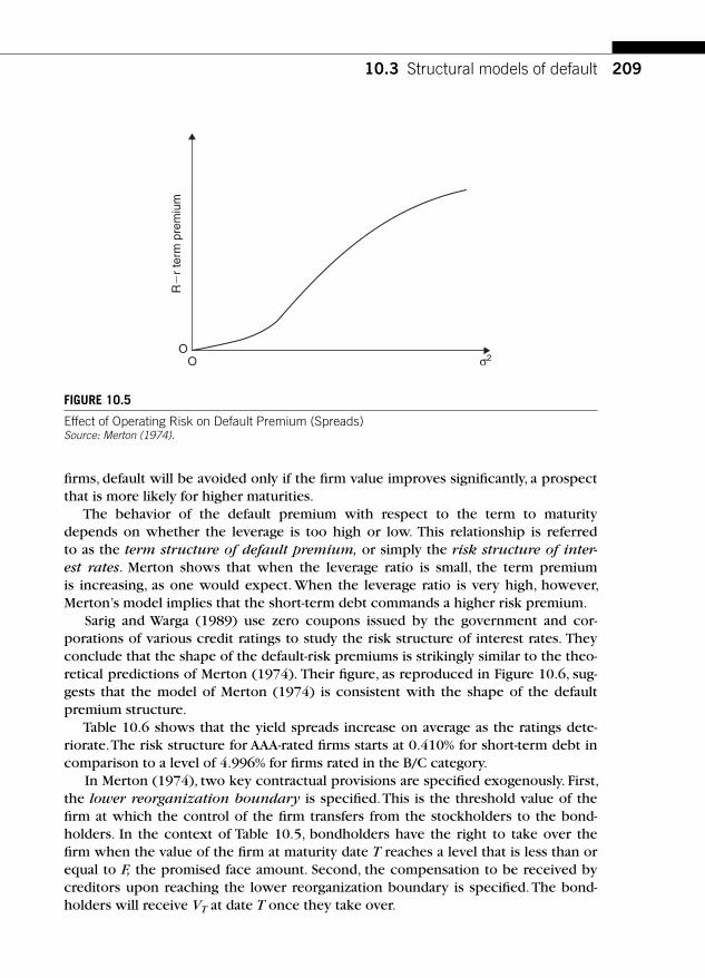
209
fi rms, default will be avoided only if the fi rm value improves signifi cantly, a prospect that is more likely for higher maturities.
The behavior of the default premium with respect to the term to maturity depends on whether the leverage is too high or low. This relationship is referred to as the term structure of default premium, or simply the risk structure of inter-est rates. Merton shows that when the leverage ratio is small, the term premium is increasing, as one would expect. When the leverage ratio is very high, however, Merton’s model implies that the short-term debt commands a higher risk premium.
Sarig and Warga (1989) use zero coupons issued by the government and cor-porations of various credit ratings to study the risk structure of interest rates. They conclude that the shape of the default-risk premiums is strikingly similar to the theo-retical predictions of Merton (1974) . Their fi gure, as reproduced in Figure 10.6 , sug-gests that the model of Merton (1974) is consistent with the shape of the default premium structure.
Table 10.6 shows that the yield spreads increase on average as the ratings dete-riorate. The risk structure for AAA-rated fi rms starts at 0.410% for short-term debt in comparison to a level of 4.996% for fi rms rated in the B/C category.
In Merton (1974) , two key contractual provisions are specifi ed exogenously. First, the lower reorganization boundary is specifi ed. This is the threshold value of the fi rm at which the control of the fi rm transfers from the stockholders to the bond-holders. In the context of Table 10.5 , bondholders have the right to take over the fi rm when the value of the fi rm at maturity date T reaches a level that is less than or equal to F, the promised face amount. Second, the compensation to be received by creditors upon reaching the lower reorganization boundary is specifi ed. The bond-holders will receive VT at date T once they take over.
OO
σ2
R�
r te
rm p
rem
ium
FIGURE 10.5
Effect of Operating Risk on Default Premium (Spreads) Source : Merton (1974).
10.3 Structural models of default

210 CHAPTER 10 Modeling credit risk and corporate debt securities
10.3.1 Probability of default and loss given default
Merton’s model provides a convenient framework for understanding probability of default and the loss given default. These two variables are crucial in determining credit spreads. The value of risky debt in Equation 10.4 can be written as follows to emphasize the role of probability of default and loss given default:
D V t Fe Fe Fe N d V N d
Fe
tr T t r T t r T t
t
r T
( ) ( ) ( )( ) ( ) ( )
(
, � � � � �
�
� � � � � �
�
2 1
�� � �
� � �
� � ��
��
� �
t r T tt
r T t r T
Fe N d VN d
N dN d
Fe Fe
) ( )
( (
( )( )
( )( )2
2
21
) �� ��
��t
tVN d
N dN d) ( )
( )( ).1
22
⎡
⎣⎢⎢
⎤
⎦⎥⎥
(10.6)
0
1
2
3
4
5
1.5 3.5 5.5 7.5 9.5 11.5 12.5�
Maturity (years)
Ris
k pr
emia
(pe
rcen
t per
ann
um)
AAA
AA
A
BBB
BB
B/C
FIGURE 10.6
Empirical Evidence on Risk Structure of Interest Rates Note: Yield spreads for corporate zero coupon bonds, February 1985 through September 1987. Maturity numbers (horizontal axis) correspond to the average maturity of each cell [in Table 10.6]. Average yield spreads are calculated as follows: In each month, the yield to an individual corporate bond has subtracted from it the yield to a zero coupon government “strip” with identical maturity. If no government strip with identical maturity existed, the yields on the two “strips” with maturities most closely bounding the corporate bond were interpolated to obtain the appropriate risk-free zero coupon yield. These yield differences were then averaged across bonds in a given month and then across time to produce the results. Source: Sarig and Warga, “Some Empirical Estimates of the Risk Structure of Interest Rates, ” Journal of Finance,December 1989, Vol. 44, No. 5, pp. 1351 –1360.

211
The last line of Equation 10.6 shows that the value of a credit-risky bond consists of three terms. The fi rst term is the present value of an otherwise identical risk-free debt. The second term is the probability of default (denoted by N ( � d 2)) multiplied by the discounted loss given default denoted by
Fe VN d
N dr T t
t� � �
�
�
( ) ( )
( )1
2
⎡
⎣⎢⎢
⎤
⎦⎥⎥.
Thus Merton’s model can be used to get quantitative assessments of loss given default as well as the probability of default. We illustrate this idea with an example.
Example 10.2 Merton’s model (see Figure 10.7 ) is based on the principle of no arbitrage and the probability of default is the risk-neutral probability of default. In real life, we need to recognize that inves-tors are risk averse, and there is a premium required for holding risky assets.
Table 10.6 Empirical Evidence on Spreads
Maturity AAA AA A BBB BB B/C Unrated
0.5 – 2.5 Years 0.410 21
0.621 74
0.775 123
1.326 48
1.670 64
4.996 41
3.081 38
2.5 – 4.5 Years 0.232 11
0.562 99
0.736 251
1.275 152
1.495 79
4.650 117
3.232 96
4.5 – 6.5 Years NA 0.620 114
0.778 221
1.405 59
2.730 58
3.365 125
3.197 119
6.5 – 8.5 Years NA 0.620 96
0.660 138
NA 1.878 51
2.959 80
3.443 119
8.5 – 10.5 Years 0.626 24
0.575 69
0.816 97
NA 0.989 10
2.912 10
3.099 88
10.5 – 12.5 Years NA 0.566 64
0.854 110
NA NA NA 2.478 64
12.5 Plus Years 0.544 64
0.544 501
0.740 510
NA NA NA 2.516 278
Yield Spreads for Corporate Zero Coupon Bonds Average yield spreads are calculated over the period February 1985 through September 1987 as follows: In each month the yield to an individual corporate bond has subtracted from it the yield to a zero coupon government “ strip ” with identical maturity. If no government strip with identical maturity existed, the yield on the two “ strips ” with maturities most closely bounding the corporate bond were interpolated to obtain the appropriate risk-free zero coupon yield. These yield differences were then averaged across bonds in a given month and then across time to produce the results reported for each cell. The unrated column contains bonds from a mixture of ratings and should not be taken to be the lowest rating group. The fi gures are in percent per annum, and the number of observations is reported below the yield.
10.3 Structural models of default

212 CHAPTER 10 Modeling credit risk and corporate debt securities
Denoting the expected return on this asset as μ, we can compute the real-life probability of default, NP ( � d � 2 ), as follows:
dln
VF
T t
T t
t
� �
� � �
�2
12
2⎛⎝⎜⎜⎜
⎞⎠⎟⎟⎟⎟ ( )( )
.μ σ
σ (10.7)
Compare Equation 10.7 with Equation 10.3 and note that d � 2 � d 2. Hence NP(� d � 2) � N(� d 2). The risk-neutral probability of default is more than the real-life probability of default.
10.3.2 Market prices
Stock prices and bond prices contain valuable information about credit risk. An increase in credit risk translates into lower equity and bond prices, ceteris paribus. Market prices change continuously. To the extent that markets are effi cient in pro-cessing information, we can expect equity prices and yield spreads to provide a bet-ter “discovery ” of credit risk than other sources.
A credit event may lead to a lower recovery rate on the loan or bond obligations. So, the investors are interested in determining the probability of default (leading to a credit event) as well as the potential recovery rates in the event that default
1011121314151617181920212223242526272829303132
�(LN(E16/E13)�(E14�E17^2/2)*E15)/(E17*SQRT(E15)
F
30%
�NORMSDIST(J15)
��J17*E16�E13*EXP(�E14*E15)*J18
�E13*EXP(�E14*E15)
�I25�I23
10.2868%YTM of risky debt � ��LN(I27/E13)/E15
0.7558%Credit spread � �I29�E14
D E F G H I J K L
Value of risky debt �
Value of put �
Value of risk-free debt �
90.2246
90.91
0.6845
Risk-neutral probability of default � N(�d2) �
N(d2)N(d1)
6.43%
0.9357 N(�d2) 0.06430.9656 N(�d1) 0.0344Sigma
V 150
T-t 1 d2
d1
1.5193
1.8193
�d2
�d1
�1.5193
�1.8193r 9.5310%
100
FIGURE 10.7
Merton’s Model

213
occurs. Together, the probability of default and the recovery rates determine the value of a credit-risky security.
10.4 IMPLEMENTING STRUCTURAL MODELS: THE KMV APPROACH
To implement structural models, we need to estimate the value of the assets of the company, which is very diffi cult. In addition, we need to fi gure out the volatility of the company’s assets. There is a way we can extract these two pieces of informa-tion from the market. We observe the equity price in the market. We know that in Merton’s model equity is a call option on the assets of the fi rm with a strike price equal to the face value of the debt. This leads to the following equation:
E VN d Fe N dr T t� � � �( ) ( ).( )1 2 (10.8)
We can also estimate or obtain the implied volatility of equity. Under some sim-plifying assumptions, we can show that the equity volatility and asset volatility are related through the leverage and the degree to which the option value to default is in-the-money. This relation is shown in the following equation:
σ σE VV
EN d� ( ).2 (10.9)
We can solve these two equations simultaneously for the values of V and the vola-tility of the assets of the fi rm. Once we have these two variables, we can estimate the probability of default from the model. First we illustrate these ideas in the context of a simple example.
Example 10.3 Let’s consider a simple example: The value of equity of a company is $3 million, and it has a single zero coupon bond outstanding with a face value of $10 million due in two years. The implied volatility of the company’s equity is 60%. Based on this information, let’s address the following questions:
● What is the implied value of the fi rm’s assets? ● What is the implied volatility of the fi rm’s assets? ● What is the probability of default by the company at maturity of the debt?
To address these questions, we use Excel to solve the two equations described earlier. This solution is shown in Figure 10.8 . The Solver function allows us to determine the value of the assets of the fi rm (11.89) as well as the volatility of the assets (16.87%). The (risk-neutral) probability of default is simply N ( � d2). In this example, the risk-neutral probability of default is 15.22%. We can compute in standardized units just how far the fi rm is from defaulting. This is the distance between the value of the assets of the fi rm (11.89) and the face value of debt (10) standardized in terms of the volatility of the asset value (16.87%). In the industry this is sometimes referred to as the distance to default . In our example it is 1.493.
10.4 Implementing structural models: the kmv approach

214 CHAPTER 10 Modeling credit risk and corporate debt securities
FIGURE 10.8
Implementing Merton’s Model Using Equity Prices

215
A company known as KMV Corporation uses the structural approach to calculate the expected default frequency (EDF) for various horizons. Equity prices are used in conjunction with the balance sheet information to estimate probability of default and distance to default. The probability of default is estimated as shown in Figure 10.8. The distance to default (DD) is computed from a model similar to Merton. Distance to default is simply the difference between the value of the fi rm and the par value of debt expressed in units of standard deviations of the fi rm’s value. Empirical evidence suggests that such measures provide good predictive informa-tion about future credit-rating changes and defaults. Credit risk monitor (which is the name of KMV’s product) is built based on this structural model’s intuition. They compute the expected default frequency (EDF), which is the probability of default for a horizon ranging from one to fi ve years.
KMV computed EDF in three steps, shown in Figure 10.9 .
1. Calculate the implied asset value and asset volatility using both the market data and the company’s fi nancial statements.
2. Estimate the distance to default, as described earlier. 3. KMV uses the historical data on defaults and bankruptcies to determine the
EDF, given the distance to default.
Marketvalueassets
Possibleasset value
path
Distributionof asset valueat the horizon
Defaultpoint
EDF
TimeH0
V0
DD
3
2
5
6
4
1
FIGURE 10.9
Conceptual Framework for Calculating EDF Source: Peter Crosbie and Jeff Bohn , Modeling Default Risk, KMV, 2003.
10.4 Implementing structural models: The KMV approach

216 CHAPTER 10 Modeling credit risk and corporate debt securities
10.4.1 Subordinated corporate debt
In an insightful paper, Black and Cox (1976) have examined the problems associated with the pricing of subordinated debt claims. We review the basics here. Consider the XYZ company in Table 10.7 and assume that it has two zero coupon issues due to mature at date T. Assume that one issue is senior with a promised face amount F 1 and another is a junior issue with a promised face amount F 2. We will continue to assume that the process of fi nancial distress and bankruptcy is costless. If we were to denote the value at date t of the equity by S, the senior bonds by B 1, and the junior bonds by B 2 , the value conservation requires that
V S B Bt � � �1 2.
We also assume that the bondholders have no recourse until date T, when their face amounts become due. (This unrealistic assumption will be removed later, and the pricing implications will become clearer.)
Table 10.7 illustrates the ideas in the pricing of subordinated debt. Note that the payoffs to the senior bondholders can be thought of as a covered call: The senior bondholders own the fi rm, but they have sold a call on the fi rm with a strike price equal to the face value F 1 of their debt security. The equity is simply a call on the assets of the fi rm, with a strike price equal to the combined value of the face amount F 1 � F 2. By value conservation, we can write the junior debt’s value as a portfolio of calls; the subordinated debt is equivalent to a long position in a call with a strike price of F 1 and a short position in a call with a strike price of F 1 � F 2. Both calls are on the assets of the fi rm with a maturity date T.
10.4.2 Safety covenants
Typically, bond covenanting may specify some net-worth constraints or safety cov-enants. For example, if at any time l, where t � l � T, the value of the fi rm Vl were to drop to a level X, the bondholders have the right to take over the fi rm and obtain a prespecifi ed compensation; the actual amount may be written down by a certain
Table 10.7 The Black and Cox Approach to Subordinated Debt Valuation
Transaction at Date t Cash Flow at Date t
V * ≤ F 1 F 1 < V * ≤ ( F 1 � F 2) V * > ( F 1 � F 2 )
Buy equity in the fi rm �S 0 0 V * � ( F 1 � F 2 )
Buy senior debt of the fi rm
� B 1 V* F 1 F 1
Buy subordinated debt of the fi rm
� B 2 0 V * � F 1 F 2

217
amount from the originally promised payments to refl ect the costliness of fi nancial distress.
Consider Table 10.8 , where there is a single issue of a zero coupon debt. Let’s modify the covenants so that the lower reorganization boundary is X. If this bound-ary is reached by the fi rm’s value before T, the bondholders get an amount Y. In this case, the stockholders have a down-and-out option. A down-and-out call option is very similar to a regular call option. Unlike a regular call option, however, a down-and-out option automatically expires when the underlying asset reaches a prespeci-fi ed low value. In the context of the corporate bond-pricing problem, stockholders have a call option, but with a safety covenant, the call becomes a down-and-out option; when the value of the fi rm reaches a low level X, the fi rm is taken over. Bondholders get Y, and equity holders get X � Y or 0, whichever is higher.
Consequently, the bondholders may be thought of as owning the fi rm but as hav-ing sold a down-and-out option to the stockholders. It is clear from Table 10.8 that the safety covenant allows the bondholders to take over the fi rm sooner if the fi rm gets into trouble.
So far, fi nancial distress has not been explicitly modeled in the pricing of corpo-rate debt. It is useful to review the empirical evidence on fi nancial distress before we examine corporate debt-pricing models that incorporate fi nancial distress.
10.5 COSTS OF FINANCIAL DISTRESS AND CORPORATE DEBT PRICING
In Merton’s model, fi nancial distress is too simply resolved: Debt holders wait until maturity, and then if the fi rm’s value is below the face value, they take over the fi rm without any costs. In reality, debt holders can be much more proactive. They may monitor the fi rm’s fi nancial health frequently before the maturity date. (Safety cov-enants and sinking funds are ways to do this.) In practice, this is achieved by requir-ing semiannual coupons. Every six months, debt holders get a chance to see whether there is enough money in the fi rm to pay coupons.
Table 10.8 Safety Covenants
Transaction at Date t Cash Flow at Date t First Date l When Vl ≤ X Safety
Covenant Is Breached
If the Safety Covenant Is Never Reached Prior to Maturity
Payoff at Maturity
Buy equity in the fi rm � S Max [0, X � Y ] V* � F
Buy senior debt of the fi rm
� B 1 Y F
10.5 Costs of fi nancial distress and corporate debt pricing

218 CHAPTER 10 Modeling credit risk and corporate debt securities
Usually, there are renegotiations and workouts. In sovereign bond markets, lend-ers often agree to reschedule the interest and principal payments. There are “debtholidays ” that are granted to enable the borrower to recover its fi nancial health. In addition, the process of fi nancial distress can be time-consuming and costly. Chapter 11 is one of the ways fi nancial distress is resolved.
Chapter 7 is invoked for liquidation. There are signifi cant direct and indirect costs of bankruptcy and fi nancial distress. Structural models with strategic defaults explore how these factors modify the predictions of Merton’s model, which is a very important benchmark in much the same way Modigliani-Miller results are in corporate fi nance. The effect of direct and indirect costs of bankruptcy implies that the borrowers and lenders will seek to avoid these wasteful costs by renegotiating loan contracts.
Over the 1926 –1986 period, the yield spreads on high-grade corporates (AAA-rated) ranged from 15 to 215 basis points and averaged 77 basis points, and the yield spreads on BAAs (also investment grade) ranged from 51 to 787 basis points and averaged 198 basis points. Such spreads can only be accounted for within the Merton model by resorting to implausibly large values of d and s V.
Most corporate securities promise coupon payments; indeed, zero coupon cor-porate securities are relatively rare, and for good reason. After all, when an investor buys a long-term bond from a corporation, he or she would like to have a periodic credible signal that the corporation is doing well and generating suffi cient cash fl ows to honor its promised coupon obligations; coupons represent such a credible signal. Sinking-fund provisions further enhance the value of the signal by requiring that the balloon payments be periodically reduced.
With a zero coupon bond, the burden of bankruptcy is placed on the principal payment at maturity and not on the coupon obligations along the way. We can think of situations in which the fi rm is illiquid and unable to meet a promised coupon. To keep the bondholders from taking over the fi rm, it may sell additional equity or resort to selling assets.
The values of Treasury and corporate bonds are infl uenced signifi cantly by inter-est rate risk. For investment-grade corporate bonds, the bulk of the risk is interest rate related and not due to credit-related factors. Jones, Mason, and Rosenfeld (1984) conclude that the introduction of stochastic interest rates might improve the perfor-mance of such models as Merton (1974) . Kim, Ramaswamy, and Sundaresan (1993) confi rm that the modeling of stochastic interest rates and cash-fl ow-triggered fi nan-cial distress can better explain the spreads between corporate and Treasury yields.
Bankruptcies and fi nancial distress are costly. Such costs have broad ramifi cations that have been ignored thus far. We will review the empirical evidence later and attempt to incorporate some of these facts into the corporate-pricing model. Central to the understanding of corporate debt is the process by which fi nancial distress is managed. This is especially important for poorly rated debt, which is subjected to a higher probability of incurring fi nancial distress. John (1993) surveys and synthe-sizes the factors pertaining to fi nancial distress. He proposes that fi nancial distress happens when the liquid assets of the fi rm are not suffi cient to meet the obligations of the fi rm’s debt contracts. Thus, fi nancial distress can be thought of as a mismatch

219
between the fi rm’s current assets and its current obligations. It can be handled in a number of ways:
1. The existing assets can be partially liquidated. This will improve the liquidity of the fi rm and stave off fi nancial distress. The disadvantage of this approach is that there are also liquidation costs (both direct and indirect).
2. The fi rm can enter into a process of negotiation with debt holders and reconfi g-ure the debt obligations. This may entail a reduction in the liabilities of the fi rm or a deferment of the payments. Such debt restructuring will involve the following: ■ Reducing the coupons and/or the principal obligations ■ Increasing the maturity of the debt ■ Accepting the equity of the company in lieu of some of the outstanding
obligations 3. The fi rm can issue additional claims to achieve the liquidity necessary to avoid
fi nancial distress.
Note that the process of managing fi nancial distress involves fi nancial reorganiza-tion either on the asset side or on the liability side or both. It can be accomplished either out of court or within the formal bankruptcy codes applicable. The traditional approach to managing fi nancial distress is for either the debtor or the creditor of the distressed fi rm to fi le for bankruptcy protection under Chapter 11. The debtor will then have the right to propose a reorganization within 120 days from the fi ling date. The process of fi nancial reorganization may involve the creditors, and the 120-day period may be extended by the court if it is deemed necessary. The plan is then eval-uated by the debt holders, who may either accept or reject it. Chapter 7 of the bank-ruptcy code is used to liquidate the fi rm if the reorganization plan is not accepted. The liquidation costs associated with court-supervised procedures can be quite high in terms of both resources and the time it takes to complete the process.
The key empirical regularities associated with fi nancial reorganizations in the 1980s are well documented. This section and the next are drawn heavily from Anderson and Sundaresan (1996). Franks and Torous (1989; 1993) fi nd the following:
■ Bankruptcies are costly because of both direct costs and disruptions of the fi rm’s activities.
■ Bankruptcy procedures give considerable scope for opportunistic behavior by the various parties involved.
■ Deviations from the absolute priority of claims are common.
All this suggests that the lower reorganization boundary of the fi rm used in Merton (1974) and in Black and Cox (1976) oversimplifi es real-life reorganizations in many important respects. In an important study, Franks and Torous (1993) point out that the costliness of the formal bankruptcy process creates an incentive for renegotiation of the distressed fi rm’s claims. They report that renegotiations result in substantial deviations from absolute priority that are not favorable to equity. In the renegotiations, some or all holders of the fi rm’s securities agree to restructure their
10.5 Costs of fi nancial distress and corporate debt pricing

220 CHAPTER 10 Modeling credit risk and corporate debt securities
claims. However, despite the incentives to do so, in practice it often proves impos-sible to renegotiate claims, resulting in formal bankruptcy and liquidation (Asquith, Gertner, and Scharfstein, 1994).
We illustrate structural models with strategic debt service using a simple exam-ple. Consider a fi rm in Figure 10.10 with an asset value of 100. In one year, the assets can have a value of 110 or 90, as shown in the following distribution. The probability of an up move is q and a down move is 1 � q.
The fi rm has a zero coupon bond maturing next year with a par value of 100. Let’s assume that if the bondholders invoke Chapter 11 or similar proceedings, it will cost them $15. If this is also known to equity holders, they will realize that the bondholders will net of all expenses the distribution shown in Figure 10.11 .
Therefore, there is an incentive for equity holders to pay no more than 95 in the good state and no more than 75 in the bad state. This is called strategic debt service.The precise amount that equity holders will pay depends on their bargaining power, their need to access the credit markets again, and so forth. The central idea, however, is that the bondholders could get less than what was promised when there are costs to fi nancial distress. Rational bondholders will anticipate this and will discount the price of corporate debt to refl ect potential strategic debt service by equity holders.
10.6 REDUCED-FORM MODELS In this class of models, we directly model the probability of default and the recovery rates. The focus of these models is the time to default. For example, we can assume
q
100
110 (good state)
90 (bad state)1 � q
FIGURE 10.10
Probability Distribution of Asset Values
110 � 15 � 95
90 � 15 � 751 � q
q
FIGURE 10.11
Probability Distribution of Payoffs to Bondholders

221
that the time to default is governed by a Poisson process, whereby the intensity of the process can depend on some exogenously specifi ed state variables. By their very nature, default is a surprise event in the reduced form models. These models can be calibrated to credit-rating information, such as migration probabilities, and are par-ticularly valuable in the pricing of credit derivatives.
For example, let’s say that default is a surprise event with a hazard rate λ. This means the following: If the fi rm survives at time t, the probability that it will default between t to t � Δ t is approximately λ Δt. Consider a very simple illustration in which we want to price a default-risky zero coupon bond with two years left to maturity. Let’s assume that the bond will pay, at date t � 2, $100 if there is no default. If there is default, the bond will pay $50; we assume a recovery of 50% of par value. Let’s assume that the probability of default at each node is 5%. Note that at date t � 1, the bond may default at either of the two nodes with a probability of 5%. We have to fi gure out what the value of the risky bond will be on date t � 1 at the up node as well as at the down node. To do this in a systematic manner, we need to specify the evolution of risk-free rates at each node of the lattice (see Figure 10.12 ). This will then allow us to discount expected cash fl ows at each node of the lattice.
Let’s further assume that the risk-free rate evolves, as shown in Figure 10.13 . With these assumptions in place, we can value the credit-risky zero coupon bond
as follows: First, we evaluate the value of the bond at date t � 1, at the top node:
Vu �� � �
�0 95 100 0 05 50
1 1187 83784
. .
.. .
Note that with 95% probability the bond would have paid $100 at date t � 2, and with 5% probability it would have paid $50. The expected payoff is discounted at the risk-free rate of 11%.
In a similar manner, we can compute the value of the bond at the lower node at date t � 1 as follows:
Vd �� � �
�0 95 100 0 05 50
1 0989 44954
. .
.. .
The yield on this risky bond can be computed at each node as follows. At the up node at date t � 1, the yield will be
100
87 837841 13 8462
..� � %.
In a similar manner, we can compute the yield of the bond at date t � 1 at the down node as
100
89 449541 11 7949
..� � %.
10.6 Reduced-form models
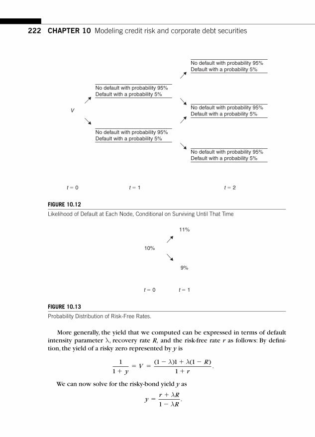
222 CHAPTER 10 Modeling credit risk and corporate debt securities
More generally, the yield that we computed can be expressed in terms of default intensity parameter λ, recovery rate R, and the risk-free rate r as follows: By defi ni-tion, the yield of a risky zero represented by y is
1
1
1 1 1
1�� �
� � �
�yV
R
r
( ) ( )λ λ.
We can now solve for the risky-bond yield y as
yr R
R�
�
�
λλ1
.
V
No default with probability 95%Default with a probability 5%
No default with probability 95%Default with a probability 5%
No default with probability 95%Default with a probability 5%
No default with probability 95%Default with a probability 5%
No default with probability 95%Default with a probability 5%
t � 0 t � 1 t � 2
FIGURE 10.12
Likelihood of Default at Each Node, Conditional on Surviving Until That Time
10%
11%
9%
t � 0 t � 1
FIGURE 10.13
Probability Distribution of Risk-Free Rates.

223
In the continuous limit, we get an intuitive relationship between risky-bond yield and risk-free rate as shown here:
y r R� � �λ( ).1 (10.10)
Equation 10.10 says that the credit risk spread is simply the risk-neutral probabil-ity of default multiplied by the loss given default. Duffi e and Singleton (1997) have developed these ideas formally and have shown several applications of this concept.
The main advantage of this approach is that we can price default-risky discount bonds as though they are default-free provided that we use the process for Rt to per-form discounting.
10.7 CREDIT SPREADS PUZZLE The models that we have presented imply the following: Credit spreads are largely accounted for by two fundamental factors: (1) probability of default, or default risk, and (2) recovery risk inasmuch as, conditional on default, lenders typically receive a fraction of their promised payments (see Table 10.2 ). Empirical evidence suggests that proxies of these two factors are typically not able to account for the changes that one observes in credit spreads. Collin-Dufresne, Goldstein, and Martin (2001) show that such proxies are unable to explain more than 25% of the fl uctuations in credit spreads.
One possible explanation might be that corporate bonds are seldom active in secondary markets, and hence secondary market trading can be very costly in terms of locating buyers/sellers in a timely fashion and in executing transactions of reason-able sizes. Though there is admittedly some liquidity premium component in cor-porate bond yields and it is not insignifi cant, it does not contribute suffi ciently to explain the levels and fl uctuations in credit spreads. This inability of credit risk mod-els to explain credit spreads has come to be known as the credit risk puzzle. Theseauthors also note that after accounting for these two factors, if one were to examine the residual returns, they are not easily explained by systematic aggregate factors such as macroeconomic variables.
To get some traction on this puzzle, we can go back to the basics of risky corpo-rate debt pricing. The price of a risky zero coupon bond at date t that pays $1 at date T can be written as follows (given the information at date t ):
z T e E P P rtr T t
T T M( ) cov( , )],( )� � � � [ [ ] λ (10.11)
where PT is the value of the zero at maturity date T. Note that the zero coupon bond will pay $1 if there is no default and will pay the recovery rate on $1 if there is default. So, the fi rst term in Equation 10.11 captures the probability of default and loss given default. The second term depends on the market price of risk, denoted by λ, and the covariance of the cash fl ow from the risky bond with market returns; if the bond pays the promised returns when the market returns are low, the risky bond
10.7 Credit spreads puzzle

224 CHAPTER 10 Modeling credit risk and corporate debt securities
price will go up and the required rate of return will go down. Defi ning the yield to maturity as y , we can write Equation 10.11 as follows:
z T e e E P P ry r P
ty T t r T t
T T M( ) [ ] cov( , )]ln[ cov(
( ) ( ) � � �� �
� � � � [ λ⇒ λ TT M Tr E P, ) ]]� [
(10.12)
The credit spread in Equation 10.12 depends on (a) the expected terminal price of the zero coupon bond, which is a function of expected recovery rates and the likelihood of default, and (b) on the market price of risk and the covariance of risky bond price with overall market return. This makes it clear that a fraction of the credit spreads must arise from risk premium demanded in the market. Since the risk pre-mium is time varying, the credit spreads must also vary over time. This idea has been formally explored to explain the observed credit spreads in Chen (2008) and Chen, Collin-Dufresne, and Goldstein (2007).
SUGGESTED READINGS AND REFERENCES Black , F. , & Cox , J. ( 1976) .Valuing corporate securities: Some effects of bond indenture provisions .
Journal of Finance , 31 , 351 – 368 .
Collin-Dufresne , P. , & Goldstein , R. S. ( 2001, December ) .The determinants of credit spread changes . Journal of Finance , 56 ( 6) , 2177 – 2207 .
Chen , H. ( 2008) . Macroeconomic conditions and the puzzles of credit spreads and capital struc-ture . Sloan School of Management, MIT .
Chen, L., Collin-Dufresne, P., & Goldstein, R. S. On the relation between the credit spread puzzle and the equity premium puzzle. Review of Financial Studies.
Merton , R. C. ( 1974) . On the pricing of corporate debt: The risk structure of interest rates . Journal of Finance , 29 , 449 – 470 .

Some fi xed income market segments
3 PART

This page intentionally left blank

227
CHAPTER
Fixed Income Markets and Their DerivativesCopyright 2009 by Academic Press. Inc. All rights of reproduction in any form reserved.
CHAPTER SUMMARY This chapter describes residential mortgage contracts. Terms such as loan-to-value ratio (LTV), fi xed-rate mortgage (FRM), adjustable-rate mortgage (ARM), and pre-payments are explained. Basic mortgage cash fl ows are derived from fi rst principles, without prepayment assumptions. Mortgage-equivalent rates are calculated using Excel. The role of federal agencies, especially the functions of government-sponsored enterprises (GSEs), are explained in detail.
11.1 OVERVIEW OF MORTGAGE CONTRACTS Home ownership in many countries is achieved through a mortgage, which is, in essence, a secured loan. The family that wants to own a home will typically pledge the home as collateral and borrow money from the lender, which is typically a bank or a fi nancial institution. Every month the homeowner will pay an amount that is credited toward the payment of interest and the outstanding principal amount that has been borrowed. In the event of a default, the lender has the right to take over the home and dispose of it in the market, to recover the outstanding balance. As we can readily see, there are two basic players in mortgage markets: lenders and borrow-ers. In addition, we will see that there are other important players, such as mortgage insurers, mortgage servicers, government agencies that have been set up to promote access to housing credit, and regulators.
More than 95% of the loans to the residential market are originated by thrifts, commercial banks, and mortgage bankers. The lending institution collects a fee for its services. This fee, known as the origination fee, is typically a small percentage of the loan. On a $200,000 loan, such a fee can be 1 point, or 1% of 200,000 � $2000. Table 11.1 records the total outstanding mortgages during the period 1Q2006 to 2Q2007.
Mortgages, federal agencies, and agency debt 11
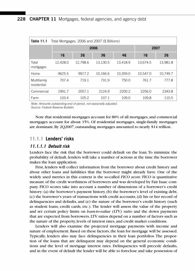
228 CHAPTER 11 Mortgages, federal agencies, and agency debt
Note that residential mortgages account for 80% of all mortgages, and commercial mortgages account for about 15%. Of residential mortgages, single-family mortgages are dominant. By 2Q2007, outstanding mortgages amounted to nearly $14 trillion.
11.1.1 Lenders ’ risks
11.1.1.1 Default risk Lenders face the risk that the borrower could default on the loan. To minimize the probability of default, lenders will take a number of actions at the time the borrower makes the loan application.
First, lenders will collect information from the borrower about credit history and about other loans and liabilities that the borrower might already have. One of the widely used metrics in this context is the so-called FICO score. FICO is quantitative measure of the credit worthiness of borrowers and was developed by Fair Isaac com-pany. FICO scores take into account a number of dimensions of a borrower’s credit history: (a) the borrower’s payment history, (b) the borrower’s level of existing debt, (c) the borrower’s years of transactions with credit accounts, (d) his or her record of delinquencies and defaults, and (e) the nature of the borrower’s credit history (such as student loans, credit cards, etc.). The lender will assess the value of the property and set certain policy limits on loan-to-value (LTV) ratio and the down payments that are expected from borrowers. LTV ratios depend on a number of factors such as the nature of the property, levels of interest rates, and credit market conditions.
Lenders will also examine the projected mortgage payments with income and nature of employment. Based on these factors, the loan for mortgage will be assessed. Typically, lenders also may face delinquencies in their loan portfolios. The propor-tion of the loans that are delinquent may depend on the general economic condi-tions and the level of mortgage interest rates. Delinquencies will precede defaults, and in the event of default the lender will be able to foreclose and take possession of
Table 11.1 Total Mortgages, 2006 and 2007 ($ Billions)
2006 2007
1Q 2Q 3Q 4Q 1Q 2Q
Total mortgages
12,428.0 12,798.6 13,130.5 13,418.9 13,674.5 13,981.8
Home 9625.5 9917.2 10,166.6 10,359.0 10,547.0 10,749.7
Multifamily residential
707.4 719.1 731.9 750.0 761.7 777.8
Commercial 1991.7 2057.1 2124.9 2200.2 2256.0 2343.8
Farm 103.4 105.2 107.1 109.0 109.8 110.5
Note: Amounts outstanding end of period, not seasonally adjusted. Source: Federal Reserve Bulletin .
229
the home. The recovery on the loan will then depend on the net proceeds that the lender is able to get by selling the home of defaulted borrowers. Thus, the level of housing prices is an important determinant of the profi tability of loans when loans go into default.
Lenders will typically also protect themselves by requiring the borrowers to obtain mortgage insurance, especially if the down payment is less than 20% of the value of the property; in other words, the LTV ratio is more than 80%. The insurance can be one of two forms. First, the borrower may take private insurance, which is a part of life insurance. In this case, in the event of the borrower’s death, the insur-ance policy will provide the mortgage payments. In the other form, the lender may require the insurance and obtain it from mortgage insurers. The cost will eventu-ally be borne by the borrower by way of a higher interest rate on the mortgage. Such insurance is a form of credit enhancement that will enable the lender to man-age the loan portfolio better, as we will see later. Major mortgage insurers include MGIC Investment Corporation, PMI Group Inc., Radian Group Inc., Old Republic International Corporation, and AIG.
11.1.1.2 Prepayments Lenders also face the prospect that borrowers may choose to refi nance their previ-ously taken loans. In the United States, by and large, there are no penalties for pre-paying a mortgage. Rational borrowers who are fi nancially able will then prepay their loans if their loan rates are higher than the rates at which they can get a mort-gage in the current market conditions. This would imply that lenders will face a rush by borrowers to prepay when mortgage rates fall; this rush would lead the lender to give up its high-interest rate mortgage loans and end up with low-interest rate mort-gage loans. Lenders might deal with such a risk in many ways: First, they will charge a higher mortgage rate to compensate them for the fact that borrowers have the option to call back the high-interest rate mortgage and refi nance them with a low-interest rate mortgage when mortgage rates drop. They may hedge their interest rate exposure, or they can sell their mortgage loan portfolios to buyers (such as federal agencies, described later in the chapter) or issue mortgage loans (such as adjustable-rate mortgages) that are less susceptible to prepayments.
Table 11.2 lists the top 10 lenders or originators of mortgages in the United States.
Note the steep drop in originations of mortgages for some lenders, notably Washington Mutual and Countrywide, due to the subprime crisis in the United States. Falling home prices during this period also led to a major downgrading of mortgage insurers during the subprime crisis in the United States.
11.1.1.3 Interest rate risk In addition to default risk and prepayments risks, general interest rate fl uctuations may also expose the lender to risks. When the interest rates go up, the key risk is not the risk of prepayments but the fact that the loan portfolio is sensitive to changes in
11.1 Overview of mortgage contracts
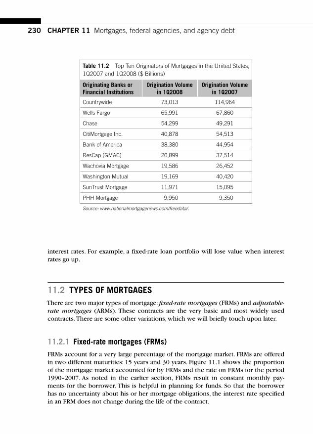
230 CHAPTER 11 Mortgages, federal agencies, and agency debt
interest rates. For example, a fi xed-rate loan portfolio will lose value when interest rates go up.
11.2 TYPES OF MORTGAGES There are two major types of mortgage: fi xed-rate mortgages (FRMs) and adjustable-rate mortgages (ARMs). These contracts are the very basic and most widely used contracts. There are some other variations, which we will briefl y touch upon later.
11.2.1 Fixed-rate mortgages (FRMs)
FRMs account for a very large percentage of the mortgage market. FRMs are offered in two different maturities: 15 years and 30 years. Figure 11.1 shows the proportion of the mortgage market accounted for by FRMs and the rate on FRMs for the period 1990–2007. As noted in the earlier section, FRMs result in constant monthly pay-ments for the borrower. This is helpful in planning for funds. So that the borrower has no uncertainty about his or her mortgage obligations, the interest rate specifi ed in an FRM does not change during the life of the contract.
Table 11.2 Top Ten Originators of Mortgages in the United States, 1Q2007 and 1Q2008 ($ Billions)
Originating Banks or Financial Institutions
Origination Volume in 1Q2008
Origination Volume in 1Q2007
Countrywide 73,013 114,964
Wells Fargo 65,991 67,860
Chase 54,299 49,291
CitiMortgage Inc. 40,878 54,513
Bank of America 38,380 44,954
ResCap (GMAC) 20,899 37,514
Wachovia Mortgage 19,586 26,452
Washington Mutual 19,169 40,420
SunTrust Mortgage 11,971 15,095
PHH Mortgage 9,950 9,350
Source : www.nationalmortgagenews.com/freedata/ .

231
11.2.2 Adjustable-rate mortgages (ARMs)
ARMs are more complicated contracts. The interest rate on an ARM changes over the life of the contract. The rates are linked to certain indexes of borrowing rates. Two indexes are widely used for setting interest rates on ARMs. They are (1) the Eleventh Federal Home Loan Bank Board District Cost of Funds Index (COFI) and (2) the National Cost of Funds Index. Indices such as LIBOR are also used. To understand ARMs better, let’s review Table 11.3 , which contains the key provisions of an ARM loan known as a 2/28.
In addition to the fact that the interest rates “ fl oat ” depending on the index levels, ARMs are frequently designed by lenders to have the following features: First, during the fi rst few years of the mortgage (ranging from one to fi ve years), the interest rate is kept at a fi xed level. Second, ARMs carry a lifetime cap on interest rates, above which the borrower will never be charged. In addition, ARMs also carry a year-to-year cap, which ensures that the borrower’s interest cannot exceed the previous year’s interest by more than a certain percentage point. Typically, ARMs will carry a margin over the index interest rates.
It should be noted that ARMs are typically indexed to short-term interest rates. We know from the evidence presented earlier in the book that short-term interest rates are much more volatile than long-term interest rates. This would therefore imply that the future monthly mortgage obligations may be much more volatile to a home-owner with an ARM.
11.2 Types of mortgages
Jan90
Jan91
Jan92
Jan93
Jan94
Jan95
Jan96
Jan97
Jan98
Jan99
Jan00
Jan01
Jan02
Jan03
Jan04
Jan05
Jan06
Jan07
Fixed-rate share (left scale)Contract rate (right scale)
0.00
2.00
4.00
6.00
8.00
10.00
12.00
0.0
10.0
20.0
30.0
40.0
50.0
60.0
70.0
80.0
90.0
100.0
Market share of fixed-rate mortgages and contract interest rate
FIGURE 11.1
Share of FRMs and FRM Rates, 1990 – 2007 Source: Daniel J. McDonald and Daniel L. Thornton, “ A Primer on the Mortgage Market and Mortgage Finance, ” Federal Reserve Bank of St. Louis Review, January/February 2008, 90 (1), pp. 31 – 45.

232 CHAPTER 11 Mortgages, federal agencies, and agency debt
Figure 11.2 shows that the ARM rate started around 2% in early January 2003 and went up steadily, all the way to nearly 4.50% by early 2007, before going down again. This level of changes in the ARMs rate can potentially lead to defaults by homeown-ers, especially when increases in ARM rates are accompanied by a slowdown in local economic conditions. Note in contrast that an FRM borrower would have locked in level payments for the life of the mortgage. ARMs have a lower prepayment risk, since the rates are indexed to market conditions. This allows the lenders to worry less about prepayment risk and focus on managing credit risk.
3/20/2003 8/1/2004 12/14/2005 4/28/2007 9/9/20081.500
2.000
2.500
3.000
3.500
4.000
4.500ARM rate
FIGURE 11.2
Eleventh District Cost of Funds Index (COFI), 2003 –2008 Source: Yield Book, Solomon Smith Barney.
Table 11.3 A 2/28 ARM Sheet
Loan type ARM. Borrower only pays interest for fi rst two years and then amortizes the balance over the remaining 28 years.
Adjustment of loan rates
Beginning in Year 3, interest rates will be reset every six months by indexing to six months ’ LIBOR at a margin of 6.50%.
Interest rates for the fi rst two years
FICO LOAN TO VALUE
45% 50% 60%
�720 10.50% 10.50% 10.50%
680 11.35% 11.50% 11.99%
620 11.90% 12.00% 12.50%
Caps Interest rates cannot go up by more than 1.5% from one year to another. During the lifetime of the loan, rates cannot go up by more than 7%.

233
Mortgage loans are also classifi ed along other dimensions, such as (a) the size of the initial loan taken, (b) LTV ratios, (c) credit scores, (d) the level of documenta-tion, (e) the ability of lenders to sell their mortgage loans to federal agencies, and (f) underwriting standards employed at the time the loan was extended.
Next we describe four types of mortgages that differ along these dimensions.
11.2.3 Agency mortgages
Agency mortgages are mortgage loans that must conform to the standards set forth by federal agencies. These standards pertain to the loan size, the borrower’s credit score, documentation, and the LTV. A mortgage is typically considered “conventional ”or “ conforming ” if the LTV ratio is small (80% or lower). Federal agencies do not pur-chase loans that exceed a certain amount. As of 2007, the maximum loan amount stood at $417,000.
11.2.4 Jumbo mortgages
Jumbo mortgages cannot be sold by lenders to federal agencies. These are relatively large loans, and the average credit quality of the borrowers tends to be high.
11.2.5 Alt-A mortgages
Alt-A mortgages are mortgages that generally conform with agency standards in terms of loan size and borrower credit score. On the other hand, these mortgages can have other unattractive features, such as low documentation.
11.2.6 Subprime mortgages
Subprime mortgages tend to have much lower FICO scores relative to agency stan-dards. They also attract borrowers who are relatively more heavily levered as mea-sured by income-to-mortgage-debt ratio, for example. In addition, the documentation on subprime mortgages tends to be much lower than agency standards. By the end of 2006, subprime mortgages grew to $1.17 trillion, accounting for nearly 12% of all mortgages.
11.3 MORTGAGE CASH FLOWS AND YIELDS As we saw in earlier chapters, bonds pay interest semiannually. Bond yields are there-fore quoted in nominal annualized terms, assuming semiannual compounding. This is known as bond-equivalent yield (BEY). On an annualized basis, semiannual BEY can be reported as follows:
Annualized YieldBEY
� � �12
12⎛
⎝⎜⎜⎜
⎞⎠⎟⎟⎟ (11.1)
11.3 Mortgage cash fl ows and yields

234 CHAPTER 11 Mortgages, federal agencies, and agency debt
Mortgages differ from bonds in several respects. First, they pay monthly cash fl ows. Second, these monthly cash fl ows include both interest payments and (amor-tizing) principal payments. Hence mortgage yields are quoted in annualized terms, assuming monthly compounding. This is called mortgage-equivalent yield , or MEY.
Annualized YieldMEY
� � �112
112⎛
⎝⎜⎜⎜
⎞⎠⎟⎟⎟⎟ (11.2)
We can compute the monthly cash fl ows of an FRM by fi rst assuming that there will be no prepayments or default, as follows: In a level-pay mortgage, each monthly payment is the same. Part of it goes toward principal and the rest toward interest. Let x be the level payments for N � 360 months. Then the present value of the sum of all these payments must be the value of the loan.
PVx
r
x
r
x
r N�
��
�� �
�( ) ( ) ( )1 1 12� (11.3)
Equation 11.3 can be simplifi ed as follows:
PVx
r r N� �
�1
1
1( )
⎡
⎣⎢⎢
⎤
⎦⎥⎥ (11.4)
Example 11.1 What is the payment of a 30-year mortgage that has a loan value of $1 million at an interest rate of 7.5% per year?
Keep in mind that a 7.5% nominal rate is 0.625% per month in simple interest. Applying Equation 11.3, we get:
$ , ,. . .
, ,1 000 0001 00625 1 00625 1 00625
62 360
� � � � �x x x
Or x( ) ( ) ( )
� ,, .992 (11.5)
Instead of solving Equation 11.5, we can directly apply Equation 11.4 as follows:
xr
r N
�
��
�
�
1 000 000
11
1
1 000 000 0 00625
11
1 006253
, , , , .
.( )
⎡
⎣⎢⎢
⎤
⎦⎥⎥
�
660
6 992⎡
⎣⎢⎢
⎤
⎦⎥⎥
� , . (11.6)
In Excel, we can use the following formula to arrive at periodic (monthly) mort-gage payments.
� � PMT ( , , ).00625 360 1000000

235
will correctly compute the value $6992. We can now split the total monthly pay-ments into an interest component and a principal component. The interest pay-ments are simply the remaining loan balance of the previous month multiplied by the monthly interest rate specifi ed in the loan. For example, in the fi rst month, inter-est payments will be $1,000,000 � 0.00625 � $6250. The principal part will then be $6992 � $6250 � $742. In the next month, the outstanding principal will be $1,000,000 � $742 � $999,258, which will be the basis for interest calculation, and so on. The results for this example are shown in the worksheet in Figure 11.3 for the fi rst 12 months. Figure 11.4 shows the cash fl ows from the mortgage for the last 12 months, assuming no prepayments.
The outstanding balance follows the relationship shown here:
B B r B xt t t� � � �� �1 1[ ] (11.7)
Equation 11.7 says that the balance this month is the previous month’s balance plus the monthly interest on the previous month’s balance minus the monthly pay-ment. In any month we can compute the principal payment as Bt� 1 � Bt and the interest payment as r � Bt� 1.
For example, let’s compute the remaining balance after 12 payments; a $1,000,000, 30-year, 7.5% mortgage with monthly payments:
PV � � ��
6992
0 006251
1
1 00625990 782
360 12. ., .
( )$
⎡
⎣⎢⎢
⎤
⎦⎥⎥
One obvious pattern is evident: In the early months, interest dominates monthly cash fl ows. On the other hand, toward the end of the life of the mortgage, principal payments dominate the monthly cash fl ows. This is shown in Figure 11.4 .
11.3 Mortgage cash fl ows and yields
FIGURE 11.3
Mortgage Monthly Cash Flows for the First 12 Months

236 CHAPTER 11 Mortgages, federal agencies, and agency debt
We sketch out the pattern of interest and principal payments in a 30-year fi xed-rate mortgage in Figure 11.5 . Keeping in mind that the monthly payments are con-stant, we observe that the earlier monthly payments are dominated by the interest component. Only around month 250 and later, principal payments begin to emerge
00
50 100 150 200 250 300 350Age in months
1,000
2,000
3,000
4,000
5,000
6,000
7,000
Interest payment Principal payment
Scheduled interest and principal payments
FIGURE 11.5
Pattern of Interest and Principal Payments in a 30-Year Fixed-Rate Mortgage
FIGURE 11.4
Mortgage Monthly Cash Flows for the Last 12 Months

237
as a signifi cant factor. These are scheduled payments; any unscheduled prepayments will of course go toward the outstanding principal. This prepayment possibility, which is at the discretion of the borrowers, is a unique and important feature of resi-dential mortgages in the United States.
In fact, in the absence of any prepayments, it takes nearly 265 months before half the original borrowed amount is repaid. This can be seen by looking at the manner in which the original borrowed amount is amortized, as shown in Figure 11.6
Of course, one of the strong incentives that the borrower will have is to try to prepay the loan if economic and other circumstances warrant it. We will investigate the determinants of prepayments later.
From the borrower’s perspective, the stated rate in the mortgage contract is the most important cost, but it’s not the only one. The borrower might have to perform an appraisal of the property, which will result in an appraisal fee. There may be costs associated with insuring the property. Other costs can include broker fees, title fees, and taxes. Once all the relevant costs are included, the effective interest rate for the borrower will exceed the stated interest rate on the mortgage. Federal regulations require that lenders disclose to borrowers the effective rate charged rather than sim-ply the stated interest on the mortgage. The effective interest rate is referred to as the annual percentage rate , or APR.
11.4 FEDERAL AGENCIES The mortgage market has two segments. One is the primary mortgage market,where borrowers get their loans from lenders. This is where new mortgages are originated or created. Mortgages that were previously originated are bought and sold
11.4 Federal agencies
1,000,000
900,000
800,000
700,000
600,000
500,000
400,000
300,000
200,000
100,000
00 50 100 150 200 250 300 350
Principal remaining
FIGURE 11.6
Principal Remaining in the Absence of Prepayments
238 CHAPTER 11 Mortgages, federal agencies, and agency debt
in the secondary mortgage markets. Both these segments have been signifi cantly changed by the presence of federal agencies. In 1932, Congress charted the Federal Home Loan Bank (FHLB) to promote mortgage fi nancing. FHLB has 12 regional banks, which meet the credit and liquidity needs of their member institutions. As of 2007, the FHLB had over 8000 members, including banks, credit unions, and insur-ance companies. Institutions such as Citibank and Countrywide are FHLB members. The FHLB provides loans and advances to its members, secured by housing collateral and the capital of members. The FHLB also has mortgage programs whereby it buys mortgages and offers fi nancing.
The FHLB is structured as a cooperative. In 1934, the FHA was set up to insure home loans. In 1938, the Federal National Mortgage Association (FNMA, also referred to as Fannie Mae) was created; its mission was to provide a secondary market for FHA and Veterans Administration (VA) mortgage loans, provide additional liquidity to the mortgage market, and improve the distribution of investment capital. Fannie Mae was set up as a wholly owned government corporation. In 1944, the VA loan guar-antee program was set up. By 1954, Fannie Mae was partly owned by private share-holders and partly by the government. In 1968, it was split into the Government National Mortgage Association (GNMA, or Ginnie Mae) and Fannie Mae. At present, Fannie Mae is a private corporation, the shares of which are listed on the New York Stock Exchange (NYSE).
The U.S. Treasury, at its discretion, may buy up to $2.25 billion worth of Fannie Mae’s debt. GNMA is wholly government owned. All its operations are fi nanced by Treasury borrowings, interest on holdings, guarantee fees, and other fees. Ginnie Mae’s mission is to supply and stimulate credit for mortgages through its secondary market activities. Ginnie Mae guarantees FHA- and VA-based mortgage-backed securi-ties (MBSs). In 1970, Congress created the Federal Home Loan Mortgage Corporation (FHLMC, also called Freddie Mac). Freddie Mac provides a link between mort-gage lenders and capital markets. It buys from savings and loan institutions, mort-gage bankers, and commercial banks and sells mortgage pass-through securities. It began with an initial capital of $100 million funded by 12 Federal Home Loan Banks through nonvoting common stock.
There are at present eight major federally sponsored agencies. Until 1987, there were only fi ve such agency issuers: the Federal Farm Credit Board (FFCB), the FHLB, Freddie Mac, Fannie Mae, and the Student Loan Marketing Association (SLMA, also referred to as Sallie Mae). The purpose of these agencies is to help promote credit availability in key sectors of the economy, such as the farm sector, housing sector, and educational sector. In 1987, the Farm Credit Financial Assistance Corporation (FCFAC) was created. The problems in the savings and loan association led to the creation of the Financing Corporation in 1987 and the Resolution Trust Corporation (RTC) in 1989. Although only the securities issued by FCFAC are backed by the full faith and credit of the U.S. Government, generally agency securities are regarded as safe securities. The credit risk in agency securities is considered to be small.
Government-sponsored enterprises (GSEs) were created to promote the availabil-ity of credit to housing. The GSEs devoted to housing are (a) Fannie Mae, (b) Freddie

239
Mac, and (c) the FHLB system. Over the last decade, GSEs have grown substantially in terms of both their issuances and the volume of debt securities that are outstanding.
The U.S. Congress charted these institutions to promote the fl ow of credit into the housing sector and to promote a liquid secondary market in residential mort-gages. These institutions have succeeded in implementing the mandate by approach-ing the problem in the following ways: Fannie Mae and Freddie Mac issue debt securities and use proceeds to buy mortgage loan portfolios from lending institu-tions. Fannie Mae and Freddie Mac are privately owned, and their stocks trade on the NYSE. As noted earlier, lending institutions will have to ensure that the loans con-form to agency standards. The knowledge that they can sell their originated loans to federal agencies will allow the lending institutions to originate the loans, sell their loan portfolios at a profi t, and resume a new cycle of lending. The presence of federal agencies increases the velocity of origination sale/origination cycle. This increases the fl ow of credit.
Together, FHLB, Fannie Mae, and Freddie Mac have had a powerful infl uence on mortgage markets. Many mortgage originators depend on Fannie Mae and Freddie Mac to purchase their originated loans in order for them to maintain relatively small balance sheets. Table 11.4 shows that the purchases of loans by these two agencies have varied from a low of 30% in 2006 to a high of 65% during the fi rst half of 2008.
Once the originating lenders sell their loan portfolios to Fannie Mae and Freddie Mac, they can choose to remain servicers of mortgages. In fact, the extent of their infl uence on mortgage markets can be best understood by reviewing Figure 11.7 .The percentage of a secondary market for mortgages held by the GSEs (right axis) was at about 80% as of 1999. The share of the GSEs fell to about 45% as of 2006 due to accounting problems at Fannie Mae and Freddie Mac as well as actions taken by the Treasury to reduce the exposure of GSEs to mortgage markets.
11.4 Federal agencies
Table 11.4 Share of Purchases of Loans by Fannie Mae and Freddie Mac (as a Fraction of Total Estimated Production of Loans), 2003 – 2008
Time Period Industry Production ($ Billions)
Purchases by Fannie Mae and Freddie Mac
($ Billions)
Market Share of Purchases (%)
FY 2003 3904 2245 57.51
FY 2004 2790 2245 57.51
FY 2005 3294 1194 36.25
FY 2006 3272 977 29.88
FY 2007 2650 1324 49.96
1H 2008 1055 687 65.21
Source: www.nationalmortgagenews.com/freedata/ .

240 CHAPTER 11 Mortgages, federal agencies, and agency debt
Figure 11.7 also shows that the market value of mortgages held by GSEs stood at about $2 trillion as of 2006. The GSEs are large, sophisticated fi nancial institutions that retain and manage credit, interest rate, and liquidity risks. GSEs earn money mainly through the following operations:
1. Credit guarantees. Fannie Mae and Freddie Mac purchase mortgages and issue mortgage-backed securities on which they guarantee the timely payment of principal and interest. As of year end 1999, guarantees by Fannie Mae and Freddie Mac totaled $1.2 trillion. These credit guarantees produce an income of about 20 basis points. On the other hand, these guarantees create contin-gent liabilities: The GSEs bear the credit risk of individual borrowers default-ing on their mortgages after losses covered by private mortgage insurance. When there is a drop in housing prices and credit becomes scarce, defaults can increase, and the obligations of GSEs to make good on their credit guaran-tees can create signifi cant liabilities.
2. Mortgage investments. GSEs purchase whole mortgages, mortgage-backed securities, and other mortgage-related securities in the capital market. By the end of 1999, the three GSEs held about $920 billion in such assets. The GSEs take on three forms of risk with these investments: credit risk, interest rate
1989 1991 1993 1995 1997 1999 2001 2003 20050
500
1,000
1,500
2,000
2,500
3,000
Bill
ions
of d
olla
rs
GSE (left scale)Private (left scale)Percent GSE (right scale)
Percentage of m
arket value held by GS
Es
0
10
20
30
40
50
60
70
80
90
100
FIGURE 11.7
Infl uence of GSEs on Secondary Markets for Residential Mortgages, 1989 –2006 Source: Daniel J. McDonald and Daniel L. Thornton, “A Primer on the Mortgage Market and Mortgage Finance, ”Federal Reserve Bank of St. Louis Review , January/February 2008, 90 (1), pp. 31 –45.

241
risk, and liquidity risk. Interest rate risk arises from prepayments, as noted ear-lier. Liquidity risk tends to be more signifi cant for GSEs because they hold a very signifi cant fraction of the secondary mortgage market; it would be very hard for them to sell parts of their portfolio without an adverse price reac-tion. If GSEs package all the mortgages that they bought and immediately sell them as mortgage-backed securities, they do not face prepayment risk. But as it stands, GSEs do own a very signifi cant amount of mortgages. One motiva-tion for owning mortgages is the spread between the income from mortgages and the costs of issuing debt to fi nance the purchase of mortgages. Jaffee (2004) reports that the spread has been approximately 80 basis points per dollar of assets for Fannie Mae and Freddie Mac and about 50 basis points for the Federal Home Loan Banks.
3. Advances. The FHLB makes secured loans, called advances, to the approxi-mately 8000 banks and thrifts that are system members. As of 2006, the FHLB had provided nearly $470 billion in loans to its members. These subsidized funds are frequently used by members to make further mortgage loans, but they are also used for nonhousing purposes. Jaffee (2004) reports that the FHL Banks earned about 20 basis points per dollar of advance.
In the early 1980s, Fannie Mae became insolvent on a mark-to-market basis. A combination of government initiatives, such as legislative tax relief and regula-tory forbearance, coupled with a decline in interest rates allowed FNMA to solve its fi nancial problems. If a similar situation were to happen today, it might lead to a signifi cant bailout by taxpayers. To avoid systemic risk, it is necessary that GSEs are subjected to the same market discipline as any other fi nancial institution. GSEs now enjoy the following benefi ts:
■ GSE debt and mortgage-backed securities are exempt from registration with the Securities and Exchange Commission (SEC).
■ The GSEs are exempt from state and local corporate income taxes. ■ The GSEs have a line of credit from the Treasury that authorizes the Treasury
to purchase up to $2.25 billion of FNMA and Freddie Mac obligations and up to $4 billion of the FHLB obligations.
■ Banks are permitted to make unlimited investments in GSEs ’ debt securities, whereas there are limits placed on their investments in any other company’s debt securities.
■ GSE securities are eligible as collateral for public deposits and for loans from Federal Reserve Banks and Federal Home Loan Banks.
■ GSE securities are lawful investments for federal fi duciary and public funds. ■ GSEs are authorized to use Federal Reserve Banks as their fi scal agents, includ-
ing issuing and transferring their securities through the book-entry system maintained by the Federal Reserve.
These advantages are signifi cant, and they make the agency securities much more attractive to institutional investors. When one recognizes that FNMA and Freddie
11.4 Federal agencies

242 CHAPTER 11 Mortgages, federal agencies, and agency debt
Mac are publicly traded companies owned by their stockholders, it is unclear as to why the benefi ts enjoyed by these agencies should continue. At the time the agen-cies were created, the infrastructure for credit to the housing sector was ill devel-oped. These agencies have done a tremendous job of improving the fl ow of housing credit. Given the current sophisticated market structure for housing credit, it is not clear that government-subsidized agencies are necessary, especially given the poten-tial for costly bailouts and the incentive to take on excessive leverage. In fact, the onset of the credit crunch and the subprime crisis beginning in August 2007 led to a dramatic decline in the fortunes of Fannie Mae and Freddie Mac. These agencies faced signifi cant losses from both their positions in mortgages as well as from the guarantees that they had extended. By September 2008, the federal government had taken these GSEs into “conservatorship ” and in effect have turned all implicit guaran-tees into explicit guarantees. These GSEs have also been given access to the discount window so that they will be able to access emergency liquidity.
11.5 FEDERAL AGENCY DEBT SECURITIES In Table 11.5 , we show the volume of agency securities that is outstanding in the market as well as the new issuances during the 1996 –2007 period. To gain some per-spective, note that the GSE security issuances during 1996 were $278 billion, increas-ing to a peak of $1268 billion in 2003. In 2007, the issuances stood at $942 billion. The amount outstanding grew from $926 billion in 1996 to $2946 billion in 2007.
Table 11.5 Federal Agency Debt, 1996 –2007 ($ Billions)
Year Agency Outstanding Agency Issuance
1996 926 278
1997 1023 323
1998 1301 596
1999 1620 548
2000 1855 447
2001 2150 941
2002 2293 1042
2003 2637 1268
2004 2745 881.8
2005 2614 669
2006 2660 747
2007 2,946 942
Source: SIFMA.

243
The size of the agency market makes it a very signifi cant part of the fi xed income securities market. In 2004 Sallie Mae was privatized, and its issuances are not included in the data after 2004. There are other agencies that do not directly issue securities but do so via the Federal Financing Bank, such as the Tennessee Valley Authority (TVA) and Ginnie Mae.
Agency issues that are not a part of noncallable benchmark programs tend to be callable. These issues are priced relative to a Treasury security of similar maturity. Often their yields are quoted as a spread over the benchmark Treasury security. The issues traded at spreads varying from 1 to 150 basis points, depending on the terms of the issue. All agency securities are regarded as virtually free from credit risk. They are rated AAA. When they are not rated, they are assumed to be of the highest quality. Though this is generally the case, the fi nancial strength of the agency is also a very important factor in determining the spread at which that agency’s debt will trade relative to the Treasury.
Many players in the market, including the U.S. Treasury, have some concerns about the growth of the agency debt market. One concern is that the spurt in the growth of the agency debt market is threatening to “crowd out ” comparable corpo-rate securities. This might in turn require that corporate debt securities offer higher spreads. The U.S. Treasury is concerned with the growth of the agency market from a public policy perspective.
11.5.1 Empirical evidence on spreads
The agencies typically trade at a spread over benchmark Treasury yields. Figure 11.8 plots the spreads between Fannie Mae 10-year debt security and Treasury 10-year note yields for the 5-year period October 2003 to October 2008. Note that the Fannie Mae debt was trading at a spread of about 40 basis points in late 2003, started
11.5 Federal agency debt securities
Jan04
Jan05
Jan06
Jan07
Jan08
20
40
60
80
100
120
140
Spr
ead
FIGURE 11.8
Fannie Mae Agency Spreads over Treasury Yields Source: Yield Book.

244 CHAPTER 11 Mortgages, federal agencies, and agency debt
compressing to about 30 basis points by the middle of 2005, and stayed around that level until January 2007. Since January 2007 the spreads have started to display a persistent increasing trend and demonstrate a great deal more volatility. The onset of the credit crunch in August 2007 contributed signifi cantly to the uncertainty about the fi nancial viability of GSEs, including Fannie Mae. Factors such as risk aversion of investors, the status of GSEs in relation to their backing by the federal government, liquidity, and taxes all contribute to the spreads.
SUGGESTED READINGS AND REFERENCES Hayre , L. (Ed.). ( 2007) . Salomon Smith Barney guide to mortgage-backed and asset-backed securi-
ties . John Wiley & Sons Inc .
Jaffee , D. ( 2003) . The interest rate risk of Fannie Mae and Freddie Mac . Journal of Financial Services Research , 24 ( 1) , 5 – 29 .
McDonald , D. J. , & Thornton , D. L. ( 2008, January/February ) . A primer on the mortgage market and mortgage fi nance . Federal Reserve Bank of St. Louis Review , 90 ( 1) , 31 – 45 .

245
CHAPTER
Fixed Income Markets and Their DerivativesCopyright 2009 by Academic Press. Inc. All rights of reproduction in any form reserved.
CHAPTER SUMMARY This chapter describes residential mortgage-backed securities (MBSs). Cash fl ows of MBSs are calculated using various prepayment conventions and assumptions used in practice. Measures of prepayments such as the constant proportional pre-payments rate (CPR) and Public Securities Association (PSA) rates are introduced in a simple setting for single mortgages and then extended to pools of mortgages. The prepayment option and the factors that infl uence prepayments are described in detail. A simple model of prepayment is presented to illustrate how MBSs are priced. The concept of the option-adjusted spread (OAS) is introduced and explained.
12.1 OVERVIEW OF MORTGAGE-BACKED SECURITIES As noted in the previous chapter, lenders sell their originated mortgage loan port-folios to institutional buyers. This occurs through a process known as securitization, which leads to the creation of mortgage-backed securities (MBSs). We will begin by providing an overview of this process. MBSs are bonds that are secured or backed by a portfolio of underlying mortgage loans. Each mortgage loan in the portfolio rep-resents the future payments of a borrower who has undertaken to make monthly mortgage payments. Such payments of individual borrowers are aggregated and are used to make interest and principal payments on MBSs. This process of creating an MBS from individual mortgage loans is called securitization.
Mortgage-backedsecurities 12

246 CHAPTER 12 Mortgage-backed securities
12.1.1 Securitization
The process of securitization, which transforms illiquid, individual mortgages into liquid mortgage-backed securities, involves several players and steps. In essence, securitization involves three important steps:
1. Pooling of individual residential mortgage loans. Individual loans originated by lending institutions such as banks and thrifts are pooled into a portfolio of suffi cient size. This pooling is necessary to create a suffi ciently large size that would be of interest to institutional investors such as asset management fi rms, pension funds, insurance companies, and the like.
2. Provision of credible guarantees. This is to ensure that payments promised by the MBS will materialize in a timely fashion.
3. Issuance of the MBS. Relying on the strength of the underlying mortgage loans and guarantees, the MBS is issued with the help of fi nancial intermediar-ies such as dealers and investment banks. These securities are then purchased by institutional investors.
Figure 12.1 explains the process of securitization in greater detail. Lenders (origi-nators) assemble a portfolio of loans and create a pool of mortgages. In creating this pool, care is exercised to preserve some homogeneity; typically the pool will have either FRMs or ARMs. Pools with FRMs are much more common. The rates prevail-ing on the FRMs will not typically differ by more than 1% to 2% so that the weighted average coupon (WAC) of the pool is a reasonable measure of the coupons of indi-vidual loans. The mortgage pool will typically have loans from same geographical
Originators Pool of mortgages
Special PurposeVehicle (SPV)
Mortgage-backedsecurities
Financialintermediaries
Institutional and retailinvestors
Rating issues(Moody’s and S&P)
Credit and liquidityenhancements
FIGURE 12.1
The Process of Securitization

247
area. All these considerations allow investors to forecast prepayments with greater accuracy. The goal of originators is to move the loan portfolio out of their balance sheet and into a special-purpose vehicle (SPV), which will issue the MBS. Once the process of securitization is completed, the originators simply become servicers of the loans.
As servicers, fi nancial institutions provide a number of functions, including (a) maintaining the status of individual loans: outstanding principal, prepayments, delinquency records, and the like; (b) collecting scheduled interest, principal pay-ments, and prepayments; and (c) handling delinquencies, defaults, and foreclosures. Servicers charge a fee ranging from 25 basis points to 30 basis points for provid-ing these functions. This servicing fee is subtracted from the WAC of the underlying mortgage loans, and the remaining amount is “passed through ” to the purchasers of these mortgage loans. As a consequence, these securities are referred to as mortgage pass-through securities.
12.1.2 Guarantees and credit enhancement
For a fee, such a standardized portfolio of pooled mortgages is then guaranteed by a federal agency (or a private entity of suffi ciently high credit reputation) against default. Such defaults may occur at the level of individual units in the pool (such as a given homeowner in a pool of mortgages) or at the level of issuers. Typical guarantee fees charged by Fannie Mae and Freddie Mac are around 25 basis points. Table 12.1 lists the federal agency guarantors and the sources of their credibility.
Since September 2008, Fannie Mae and Freddie Mac have been brought under “ conservatorship ” of the federal government and their debt obligations may now be regarded as having the direct backing of the federal government. The total fees (ser-vicing and guarantees) may be on the order of 50 basis points to 75 basis points, and this comes out of the cash fl ows generated by the loan portfolio that has been moved into the SPV. The SPV is created solely to create the pool of fi nancial assets and then issue the asset-backed securities. The key idea here is to put some distance between the originators and the pool of assets. “Bankruptcy remoteness ” is the goal. In other words, the SPV is structured such that the bankruptcy of the originator(s)
12.1 Overview of mortgage-backed securities
Table 12.1 Guarantors for GSEs *
Government National Mortgage Association, or GNMA, established in 1968
Backed by full faith and credit of the U.S. Government.
Federal National Mortgage Association, or FNMA, established in 1938
Implicit guarantees; line of credit to the U.S. Treasury
Federal Home Loan Mortgage Corporation, or FHLMC; 1970
Implicit guarantees; line of credit to the U.S. Treasury
* Since September 2008, all GSEs have direct backing of the U.S. Government.
248 CHAPTER 12 Mortgage-backed securities
does not affect the pool of fi nancial assets held by the SPV. This separation is criti-cal to obtaining the necessary credit enhancements, which usually lead to a high credit rating. The structure of the collateral may itself provide some credit enhance-ment; for example, there may be “overcollateralization ” of mortgage loans that back the pass-through securities.
This process of pooling, standardizing, and selling claims on guaranteed loans has the effect of improving the liquidity of what might otherwise be illiquid assets.
The following is a comparison of the agencies and their pass-through securities:
1. GNMA. GNMA, or Ginnie Mae, fi nances FHA and VA loans. Typically the loans are from single-family, low-income households. GNMA pass-through securi-ties are guaranteed by GNMA and are issued by GNMA-approved originators and servicers. The loans are packaged in sizes of 1 million or more and placed with a trustee. Upon acceptance of loan documentation, GNMA assigns a pool number that identifi es the security to be issued. The originator or the servicer then issues pass-through securities, which are sold to investment bankers for distribution. GNMA tends to require a greater degree of homogeneity of the mortgages within a given pool. Pools tend to have a single type (single-family, 30-year fi xed, for example), and the mortgages carry the same interest rate. For single-family pools, the mortgage interest is 50 basis points higher than the pass-through rate; the 50 basis points cover the servicing fee and the guarantee fees. In the GNMA II program, there is more diversity in the underlying loans. Also under the GNMA II program, a central paying and transfer agent consoli-dates all the payments to the security holders in one monthly check, but there is a delay associated with this process.
The GNMA guarantee of full and timely payment of interest and principal is backed by the full faith and credit of the U.S. Government. GNMA covers low-income homes (house price less than $152,000). Historically, prepayments are less volatile relative to other agency pass-through securities.
2. FNMA. This agency’s stocks trade in the NYSE. FNMA buys conventional mort-gages and operates a swap program whereby loans of any age can be swapped into FNMA-issued participation securities. Such a swap can be benefi cial to the lenders in the sense that the lenders can use the FNMA-issued securities as collaterals in reverse repurchase agreements. FNMA also provides the guarantee of full and timely payment of interest and principal, but this guarantee is not backed by the full faith and credit of the U.S. Government. However, FNMA does have a $2.25 billion credit with the U.S. Treasury. FNMA pools are much more heterogeneous compared to the pools in the GNMA. FNMA pools may have mortgages with rates that vary by more than 200 basis points, and the loans may be new or seasoned. FNMA covers both FHA and VA loans as well as conventional loans, which have a much higher value. Due to this and the greater diversity of loans, prepayments are much more volatile.

249
3. FHLMC. This agency also buys FHA, VA, and conventional mortgages and oper-ates a swap program whereby loans of any age can be swapped into Freddie Mac-issued participation securities. As noted earlier, such a swap can be benefi -cial to the lenders in the sense that the lenders can use the Freddie Mac-issued securities as collaterals in reverse repurchase agreements. FHLMC also provides the guarantee of full and timely payment of interest and principal. This guaran-tee, however, is not backed by the full faith and credit of the U.S. Government, but Freddie Mac has a $2.25 billion credit with the U.S. Treasury. Freddie Mac pools are much more heterogeneous compared to the pools in the GNMA. Freddie Mac pools may have mortgages with rates that vary by more than 200 basis points, and the loans may be new or seasoned. FHLMC buys FHA and VA as well as conventional loans, which have a much higher value. Due to this and the greater diversity of loans, prepayments are much more volatile.
4. Private labels. These are nonagency pass-through securities that create a sec-ondary market for nonconforming loans, which are conventional loans that fail to meet the size limits and other requirements placed by the agencies. Private pass-through securities trade at a spread over the agency pass-through.
12.1.3 Creation of an agency MBS
Only FHA and VA loans qualify for conversion to GNMA pass-through MBSs. The loan pool must have some standard features in terms of coupon, single-family or multifamily, maturity, and so on. The minimum size of the pool is $1 million for single-family loans. GNMA II permits mortgages with different interest rates to be included in the same pool.
The following steps are taken in issuing mortgage-backed securities:
1. The originators forward the loan portfolio to GNMA with the appropriate documentation, requesting GNMA’s commitment to guarantee the securities to be backed by the pooled mortgage portfolio.
2. GNMA reviews the application. If the review is favorable, a pool number is assigned and the commitment is issued.
3. The originators transfer the mortgage documents to custodial agents and send the required pool documents to GNMA.
4. Anticipating the issuance of the GNMA guarantee, the originators solicit advance commitments from dealers, investment banks, and so on, to sell a specifi ed amount of the securities at a set price and yield.
5. GNMA reviews the documentation and issues the guarantee. The originators continue to service the loans: collecting the monthly interest and principal payments, remitting the net amount of the servicing fee to the security hold-ers, and issuing monthly account statements.
GNMAs are not debt obligations of the issuers. They represent real estate assets. The servicers collect 50 basis points per annum of the outstanding principal balance
12.1 Overview of mortgage-backed securities

250 CHAPTER 12 Mortgage-backed securities
of each mortgage for servicing and the GNMA guarantee. GNMA gets 6 basis points per annum of 50 for its guarantee.
12.1.4 Cash fl ows and market conventions
In principle, the cash fl ows (scheduled interest, principal, and prepayments) from the underlying pool of mortgages are passed through to the investors in the mortgage-backed security with the exception of fees. Servicing fees and guarantee fees will be subtracted from the cash fl ows generated by the loan portfolio that is backing the mortgage-backed security. These fees vary from one agency security to another. Homeowners tend to make their scheduled payments during the fi rst half of each month. The payments to the investors in mortgage-backed securities occur on the 15th of the next month. Market participants refer to this as a 45-day delay. This delay varies from one agency security to another. In reality, the actual delay is a good deal less than that. GNMAs are quoted in 32 nds, similar to Treasury securities. The prices quoted refer to percentages of the outstanding principal balance in the underlying pool. This requires the calculation of the outstanding balance, which in turn requires compilation of the scheduled interest and principal payments as well as any prepay-ments. For these computations, the servicing institutions calculate a pool factor. The term pool factor pf t( ) is defi ned as follows:
aiSD M
Bt ��
� � �30
1
12c
where SD is the settlement date, M is the fi rst day of the month within which t falls, B is the principal balance, and c is the coupon rate.
Let’s assume that the coupon rate c � 9% and that SD � M is 20 days. Then the accrued interest is
ait � � � � �20
309
1
1210 000 90 000, , .
Note that the accrued interest calculations differ from Treasuries in important ways. First, interest accrues from the fi rst day of the month; in Treasury markets, the last coupon date is the relevant date from which interest accrues. In the case of GNMA, the convention is actually over 360, as the example illustrates. Note that this means that an investor buying a GNMA in April for settlement in the middle of April (say, April 15) is buying a pro rata share in the outstanding principal balance of a mort-gage pool as of the end of March. This investor will expect to receive on May 15 the interest on the balance, computed as of the end of March, plus any prepayments during the month of April. When agency pass-through securities are traded, they are identifi ed with some key characteristics of the underlying pool. A pool number is assigned that enables investors to learn about the features of the underlying pool, such as whether the pool is fi xed or adjustable, the issuer, and the weighted-average coupon. Sometimes trades in securities occur before key features of the underlying

251
pool become available. Such trades are referred to as TBA (to be announced) trades. In TBA trades, investors do not know the pool numbers on the trade date, but they will know them before the settlement date.
12.2 RISKS: PREPAYMENTS Mortgages in the United States permit the homeowners to prepay their loans. This prepayment provision introduces timing uncertainty into the originating bank’s cash fl ows from its loan portfolio. For example, if the bank originates a pool of mortgages with a weighted-average rate of 8% and six months later the mortgage rates drop signifi cantly below 8%, say to 7%, then the loan portfolio is certain to experience signifi cant prepayments as borrowers rush to refi nance their mortgages with less costly loans. The lender has a long position in the mortgage loan that entitles him or her to monthly scheduled payments, but the lender has also sold an option to the homeowners that gives them the right to prepay the loan when the circumstances demand it. This means that the bank cannot predict with certainty the future cash fl ows from its loan portfolio. Clearly, the option to prepay will be priced into the loan by the bank, and the borrower will pay a higher interest rate on the loan as a consequence.
12.2.1 Measuring prepayments
Various measures of prepayments are used in the industry to determine the rate of prepayment. These measures are grounded in certain assumptions that must be understood by investors in the mortgage markets. Here we discuss each of these mea-sures in turn. All these measures have been developed in the context of mortgage-backed securities. However, they are useful even at the level of individual loans.
12.2.1.1 Twelve-year retirement This is perhaps the simplest and the least important measure of prepayment. It assumes that the mortgage is prepaid exactly after 12 years. If this assumption is made, at the end of 12 years we can add the prepayments to the scheduled pay-ments. The cash fl ows of the mortgage loan in the absence of default can then be determined for all future months. This measure is clearly inconsistent with what we know about the factors that determine prepayments.
12.2.1.2 Constant monthly mortality This measure assumes that there is a constant probability that the mortgage will be prepaid following the next month’s scheduled payments. For instance, consider the assumption that there is a 0.50% probability that the mortgage will be prepaid fol-lowing the fi rst month. This 0.50% probability is referred to as the single monthly mortality, or SMM, rate. Using the SMM, we can compute the probability that the
12.2 Risks: Prepayments

252 CHAPTER 12 Mortgage-backed securities
mortgage will be retired in the next month. It depends on two factors: (a) the prob-ability that the mortgage will survive the fi rst month, 1 � 0.50% � 99.50%, and (b) the mortality rate for Month 2 (given that it survived the fi rst month), which is 0.50%. So, the probability that the mortgage will be retired in Month 2 is 0.50% � 99.50% � 0.4975%. Using this information, we can say that the probability that the mortgage will be retired in Month 3 is (1 � 0.4975%) � 0.50% � 0.4975%, and so on. Usually an annual prepayment rate known as the conditional prepayments rate (CPR) is used to measure the speed of prepayments. Given an annual CPR, we can estimate the SMM. Remember that the probability that the mortgage will sur-vive a month is (1 � SMM). For a period of one year, the probability of survival is ( )1 12� SMM This is set equal to (1 � CPR). So, we get:
( ) .1 112� � �SMM CPR
From this we can write
CPR SMM� � �1 1( )12.
If SMM � 1% (per month), CPR is 11.36%. In our example, SMM � 1% implies that 1% of the outstanding principal is paid down each month. This measure (CPR) is used widely in the industry to measure prepayments. As the constant of monthly mortality increases, the probability that the mortgage will be retired early increases; this is useful for computing the prepayments associated with a loan portfolio. Note that this approach is inconsistent with the fact that the prepayment increases during the fi rst few years, then stays at a relatively low level and increases again toward the end of the loan period.
12.2.2 FHA experience
The Federal Home Administration (FHA) has a large database on actual prepayments of mortgages of various vintages. These data form the basis for computing the prob-ability that a loan will be retired during any given year. The probability is computed as follows: The FHA data are organized as a series, giving the probability that the new mortgage will survive to the end of any given year, where years are indexed from 1 to 30. Let xt be this probability. Then the probability that the mortgage will be retired during any given year t is
p x xt t t� ��1 .
The conditional probability that the mortgage will survive through the year t, given that it has survived until the year t � 1, is denoted by yt , and is computed as
yp
x
x
xtt
t
t
t
� � �� �
11 1
.

253
Once we have the conditional probability yt of a mortgage surviving through the year t, given that it has already survived through year t � 1, we can use that information to derive the conditional monthly survival probabilities by invoking additional assumptions about the monthly probabilities. For instance, if we assume that the conditional monthly probabilities within each year are constant (say, zi for year i ), we must have z y zi i i i
12 1 12� �⇒ y / . These derived monthly probabili-ties are referred to as the 100% FHA experience. Unlike the CPRs, the 100% FHA experience does not decline with the age of the mortgage. For example, let’s say that 58% of the mortgage pool is expected to survive 10 years and 54% of the pool is expected to survive 11 years. Using this estimate, we can compute that the pre-payment in the 11 th year will be 4%, assuming the 100% FHA experince. Investors use this information and adjust it for various speeds (i.e., 50% FHA experience, 200% FHA experience).
12.2.3 PSA experience
The Public Securities Association (PSA) convention assumes that 0.2% of the prin-cipal is paid in the fi rst month and will increase by 0.2% in each of the following months, fi nally leveling out at 6% until the maturity. This convention is referred to as the 100% PSA. By scaling up or down, we can construct different PSA measures. Figure 12.2 shows the prepayment rates for 100% PSA, 150% PSA, and 200% PSA. The PSA standard benchmark was introduced in July 1985. It is not a model of prepayments but is used as a benchmark in the industry. Mathematically, a 100% PSA
12.2 Risks: Prepayments
00.00
2.00
4.00
6.00
8.00
10.00
12.00
14.00
50 100 150 200 250 300 350 400
% P
rinci
pal p
aid
Age of mortgage (in months)
100% PSA 150% PSA 200% PSA
PSA prepayment conventions
FIGURE 12.2
PSA Prepayment Conventions
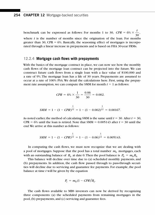
254 CHAPTER 12 Mortgage-backed securities
benchmark can be expressed as follows: For months 1 to 30, CPRt
� �630
% ,
where t is the number of months since the origination of the loan. For months greater than 30, CPR � 6%. Basically, the seasoning effect of mortgages is incorpo-rated through a linear increase in prepayments and is based on FHA 30-year FRMs.
12.2.4 Mortgage cash fl ows with prepayments
With the basics of the mortgage contract in place, we can now see how the monthly cash fl ows of the mortgage loan contract can be projected into the future. We can construct future cash fl ows from a single loan with a face value of $100,000 and a rate of 9%. The mortgage loan has a life of 30 years. Prepayments are assumed to occur at a rate of 100% PSA. We detail the calculations here. First, using the prepay-ment rate assumption, we can compute the SMM for month t � 1 as follows:
CPR � � � �61
30
0 06
300 002%
.. .
SMM CPR� � � � � � �1 1 1 1 0 002 0 001671
12( ) ( )1
12 . . .
As noted earlier, the method of calculating SMM is the same until t � 30. After t � 30, CPR � 6% until the loan is retired. Note that SMM � 0.005143 after t � 30 until the end. We arrive at this number as follows:
SMM CPR� � � � � � �1 1 1 0 06 0 0051431
12( ) (1 )1
12 . . .
In computing the cash fl ows, we must now recognize that we are dealing with a pool of mortgages. Suppose that the pool has a total number m0 mortgages, each with an outstanding balance of B0 at date 0. Then the pool balance is P m B0 0 0� .
This balance will decline over time due to (a) scheduled monthly payments, and (b) prepayments. In addition, the cash fl ow passed through to pass-through securi-ties will decline due to servicing and guarantee fee payments. For example, the pool balance at time t will be given by the equation
P m CPR Btt
t� �0 1( ) .
The cash fl ows available to MBS investors can now be derived by recognizing three components: (a) the scheduled payments from remaining mortgages in the pool, (b) prepayments, and (c) servicing and guarantee fees.
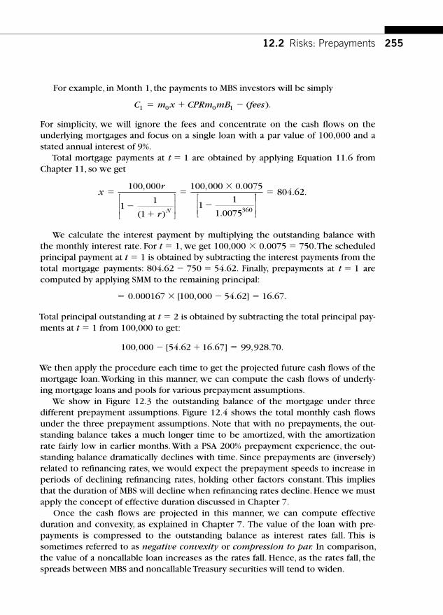
255
For example, in Month 1, the payments to MBS investors will be simply
C m x CPRm mB fees1 0 0 1� � � ( ).
For simplicity, we will ignore the fees and concentrate on the cash fl ows on the underlying mortgages and focus on a single loan with a par value of 100,000 and a stated annual interest of 9%.
Total mortgage payments at t � 1 are obtained by applying Equation 11.6 from Chapter 11, so we get
xr
r N
�
��
�
�
100 000
11
1
100 000 0 0075
11
1 0075360
, , .
.( )
⎡
⎣⎢⎢
⎤
⎦⎥⎥
⎡
⎣⎢⎢
�
⎤⎤
⎦⎥⎥
� 804.62.
We calculate the interest payment by multiplying the outstanding balance with the monthly interest rate. For t � 1, we get 100,000 � 0.0075 � 750. The scheduled principal payment at t � 1 is obtained by subtracting the interest payments from the total mortgage payments: 804.62 � 750 � 54.62. Finally, prepayments at t � 1 are computed by applying SMM to the remaining principal:
� � � �0 000167 100 000 54 62 16 67. , . . .[ ]
Total principal outstanding at t � 2 is obtained by subtracting the total principal pay-ments at t � 1 from 100,000 to get:
100 000 16 67 99 928 70, . , . .� � �[54.62 ]
We then apply the procedure each time to get the projected future cash fl ows of the mortgage loan. Working in this manner, we can compute the cash fl ows of underly-ing mortgage loans and pools for various prepayment assumptions.
We show in Figure 12.3 the outstanding balance of the mortgage under three different prepayment assumptions. Figure 12.4 shows the total monthly cash fl ows under the three prepayment assumptions. Note that with no prepayments, the out-standing balance takes a much longer time to be amortized, with the amortization rate fairly low in earlier months. With a PSA 200% prepayment experience, the out-standing balance dramatically declines with time. Since prepayments are (inversely) related to refi nancing rates, we would expect the prepayment speeds to increase in periods of declining refi nancing rates, holding other factors constant. This implies that the duration of MBS will decline when refi nancing rates decline. Hence we must apply the concept of effective duration discussed in Chapter 7.
Once the cash fl ows are projected in this manner, we can compute effective duration and convexity, as explained in Chapter 7. The value of the loan with pre-payments is compressed to the outstanding balance as interest rates fall. This is sometimes referred to as negative convexity or compression to par. In comparison, the value of a noncallable loan increases as the rates fall. Hence, as the rates fall, the spreads between MBS and noncallable Treasury securities will tend to widen.
12.2 Risks: Prepayments

256 CHAPTER 12 Mortgage-backed securities
100,000
200,000
300,000
400,000
500,000
600,000
700,000
800,000
900,000
1,000,000
00 60 120 180 240 300 360
Bal
ance
out
stan
ding
Outstanding principal and speed of prepayments
No prepayments PSA 50% PSA 200%
Age of mortgage
FIGURE 12.3
Outstanding Balance Under Three Prepayment Assumptions
0 60 120 180 240 300 360
Cas
h flo
ws
Total monthly cash flows
Age of loan in months
PSA 50% PSA 200%No prepayments
7,5007,0006,5006,0005,5005,0004,5004,0003,5003,0002,5002,0001,5001,000
5000
FIGURE 12.4
Total Monthly Cash Flows Under Three Prepayment Assumptions

257
12.3 FACTORS AFFECTING PREPAYMENTS Prepayments of mortgages are driven by a number of factors, each of which merits further elaboration.
12.3.1 Refi nancing incentive
Perhaps the most important reason for prepayments is the refi nancing incentive. If the market rates for mortgage loans drop signifi cantly below the rate that a borrower is paying, the borrower has a very strong reason to prepay as long as the borrower is able to qualify for a new loan. This incentive means that the prepayments accelerate in periods of falling interest rates, especially when there is a belief in the market that the rates have bottomed out (see Figure 12.5 ).
12.3.2 Seasonality factor
Families typically do not move during the school year. Things remaining equal, families typically move during the period from the middle of June through the fi rst week of September; this results in increased prepayments during this part of the year. This can be thought of as the seasonality factor or the school-year factor. Figure 12.6 clearly shows a strong seasonal pattern in the sale of existing homes. Such sales will result in prepayments and thus induce a seasonal effect in prepayments.
12.3 Factors affecting prepayments
70
60
50
40
30
20
10
0
CP
R (
%)
Jan 87 Jun 88 Nov 89 Apr 91 Sep 92 Feb 94 Jul 95 Dec 96 May 98 Oct 99 Mar 01 Aug 02 Jan 04
5
6
8
9
10
11
12
7 Mor
tgag
e ra
te (
%)
Fannie Mae 1987 8s CPR
Freddie Mac survey rate
FIGURE 12.5
Mortgage Prepayments and the Effect of Refi nancing Rates, January 1987 – January 2004 Source: Anatomy of Prepayments: Citigroup Prepayments Model, Salomon Smith Barney, Fixed Income Research, March 2004.

258 CHAPTER 12 Mortgage-backed securities
12.3.3 Age of the mortgage
During the early part of the mortgage loan, interest payments far exceed the prin-cipal component. This, in part, means that the interest savings associated with refi -nancing are greater during the earlier part of the mortgage loan. We expect the prepayments to be greater during the earlier part of the life of the loan and then stabilize afterward; indeed, prepayments are higher when the life of the loan is in the range of two to eight years. This is sometimes referred to as the seasoning ramp. In addition, when a mortgage is more than 25 years old, there may be an incentive to pay it off to secure the property’s title. The speed of prepayments slows for loans in the age range 10 –25 years. This seasoning effect is shown in Figure 12.7.
12.3.4 Family circumstances
A number of factors pertaining to mortgage holders ’ family circumstances lead to prepayments. These factors include marital status (divorce decisions often lead to prepayment) and job switching. Sometimes a household’s inability to make the monthly payment (due to job loss or disability) leads to default; under some circum-stances, this can precipitate a prepayment.
As noted earlier, there are two forms of mortgage insurance. In one form, the lender initiates the insurance and the policy guarantees that the insurance company will pay some or all of the loan in the event the homeowner defaults. In the other
700
600
500
400
300
200
100
01995 1996 1997 1998 1999 2000 2001 2002 2003 2004
Una
djus
ted
sale
s (t
hous
ands
)
FIGURE 12.6
Seasonality in Sales of Existing Homes, 1995 –2004 Source : Anatomy of Prepayments: Citigroup Prepayments Model, Salomon Smith Barney, Fixed Income Research, March 2004.

259
form, initiated by the homeowner, the insurance company will pay off the loan obli-gations in the event of a death of the insured person. Further, if a family moves (due to such factors as increasing family size or a job change) and if the loan is assumable, then when the family moves, the next family that moves into the home can assume the mortgage. If the loan is not assumable, it has to be paid in full, which results in prepayments. It should be noted that most mortgages in the United States are not assumable.
12.3.5 Housing prices
The price of a home is yet another factor in prepayments. The housing price affects the LTV ratio, which in turn affects a household’s ability to qualify for refi nancing. When housing prices increase, the LTV decreases. This enhances the homeowner’s ability to refi nance if the going interest rates and family circumstances warrant refi nancing. On the other hand, when the housing prices drop, the LTV ratio increases; this diminishes the homeowner’s ability to qualify for refi nancing, even if other factors favor refi nancing.
12.3.6 Mortgage status (premium burnout)
The relationship between the contractual interest rate in a mortgage loan and the going mortgage interest rates is a major determinant of the value of the loan. If the contractual interest rate r is greater than the going interest rate R, the loan is a prime
12.3 Factors affecting prepayments
125% PSA
00 5 10 15 20 25 30 35 40 45 50 55
2
4
6
8
10
12
14
CP
R (
%)
Loan age (months)
FIGURE 12.7
Seasoning Effects on Prepayments Source: Anatomy of Prepayments: Citigroup Prepayments Model , Salomon Smith Barney, Fixed Income Research, March 2004.

260 CHAPTER 12 Mortgage-backed securities
candidate for prepayment. Such mortgages are referred to as premium mortgages. If r � R, the mortgage is said to be a discount mortgage. We would expect premium mortgages to prepay faster. There is some empirical evidence indicating that the pre-mium mortgages, after some prepayments, tend to stabilize. An initial drop in rates leads to signifi cant prepayments. A subsequent drop does not produce a similar level of prepayments. Hence, a number of premium mortgages remain outstanding. This is referred to as premium burnout.
12.3.7 Mortgage term
Evidence suggests that the rate of prepayments depends on other factors as well. For example, the rate of prepayment of FRMs with a maturity of 15 years differs from the rate of prepayment of FRMs with a maturity of 30 years. Waldman, Schwalb, and Feigenberg (1993) present the following evidence: For current coupon and dis-count coupon securities, prepayments from 15-year mortgages have been 11% faster than 30-year mortgages during the period 1983 to 1992. For high-coupon securities, prepayments from 15-year mortgages have been 5% slower than 30-year mortgages during the period 1986 to 1992. The seasoning of the mortgage appears to have a signifi cant impact on the speed of prepayments.
12.4 VALUATION FRAMEWORK The basic insight into the valuation of mortgage-backed securities is to recognize that default-free assumable mortgage-backed securities consist of an annuity and a call option that gives the homeowners the right to buy the annuity at a strike price equal to the remaining par amount at any time prior to maturity (from 15 to 30 years). Thus, the factors that determine the value of a fi xed-rate mortgage are the fol-lowing: (a) coupon, (b) time to maturity, (c) amortization schedule, and (d) interest rates on comparable mortgages at the time of valuation.
The models for valuing mortgage-backed securities, such as Dunn and McConnell (1981), apply the principles of options pricing. Buser, Hendershott, and Sanders (1990) have extended the basic insights, but the principles of valuation have remained the same. Such valuation models allow for the following economic implications:
■ The expected holding-period return on any mortgage is equal to the instanta-neous riskless rate plus a risk premium.
■ Mortgage-backed securities are assumed to obey certain boundary condi-tions dictated by the economics of their valuation. For example, the value of the mortgage-backed security must satisfy two conditions: As the mortgage-backed security approaches its maturity date, its value will go to zero. This is due to the fact that the mortgage is an amortizing asset. Moreover, as the inter-est rates approach very high values, the value of the mortgage-backed security

261
approaches zero. The intuition here is that the mortgage loans are worthless at very high interest rates.
■ The fact that mortgage-backed securities are sold on mortgages that can be prepaid means that we need to impose a condition on the optimal exercise of this prepayment option. We know that the homeowners will tend to prepay the loans when refi nancing interest rates decrease to a critical low level. At that point they will prepay, and hence the security will sell at the outstanding balance or the par value when this critical refi nancing rate is reached. The exis-tence of the prepayment feature means that the value of the mortgage-backed securities behaves differently at low interest rates. This behavior is sometimes referred to as compression to par or negative convexity.
In the valuation of mortgage-backed securities, we have thus far treated interest rates as the only variable affecting the value of the security and have assumed that the mortgage-backed security is default-free. In reality, the fact that some homeowners might default affects the pricing of mortgage-backed securities. If the mortgage-backed security is fully insured and assumable (such as GNMAs), then upon default the guarantor will pay off the mortgage. Thus, the cash fl ows to mortgage-backed securities are affected by default. For example, defaults that occur during periods of very high interest rates tend to produce a gain for the security holders. When rates are high, the mortgage-backed securities sell below par, but default produces a cash fl ow equal to par, leading to a windfall gain. It is also useful to recognize the incen-tives to voluntary default that the homeowner might have. If the value of the house is relatively high compared to the value of the mortgage, the homeowner might not want to default. If the value of the house is well below the value of the mortgage, the incentive to default is high. This may be thought of as a put option or a walk-away option. Basically, when the price of the house drops to a critical low value, it is opti-mal for the homeowner to default on the mortgage. More recent models of valuing mortgage-backed securities incorporate the house price as a second factor infl u-encing the value. In such models, the value of the mortgage-backed security will be written as a function of both interest rates and house prices. Note that when house prices are low, even though the interest rates may be low, there is less incentive to prepay the mortgage; the mortgage value may exceed the house value by such a sig-nifi cant amount that the homeowner fi nds it suboptimal to exercise the option. This suggests that in periods of falling housing prices, the level of prepayments ought to go down. Our arguments suggest that housing prices affect the valuation in two dis-tinct ways:
1. At low housing prices, there is a greater incentive to default. 2. At low housing prices, the incentive to refi nance also goes down.
In addition, housing prices enable us to model situations in which depressed house prices, though not inducing immediate default, diminish the incentives to refi nance. Transaction costs in a given pool are yet another feature that we need to incorporate in the valuation framework.
12.4 Valuation framework

262 CHAPTER 12 Mortgage-backed securities
Homeowners spend time and resources in their refi nancing decisions. Title fees, appraisal fees, and so on constitute direct costs. There are signifi cant indirect costs as well, including the time spent in the choice of the mortgage loan and its analysis. It is possible that such transaction costs are dependent on the household and its cir-cumstances. Thus, if the pool has a diverse set of homeowners and their transaction costs are distinct, the prepayments from such a pool might not be easy to estimate. Note also that transaction costs are incurred by the households but are not received by the investors of mortgage-backed securities.
Although the conditions that we have laid out are intuitive, they do not necessar-ily account for values and prepayments that one observes in real life. For example, the following empirical regularities have been reported with respect to mortgage prepayments but are not accounted for in our framework:
■ Prepayment rates for deep discount securities increase over time. ■ Prepayment rates for aged premium securities decline over time. ■ Prepayment rates on newly originated mortgages increase at fi rst and then
decline.
Furthermore, prepayments, as noted earlier, depend on many factors. It is necessary to modify the framework to obtain a model of valuation that admits these regulari-ties and the richness that prepayments exhibit.
12.5 VALUATION OF PASS-THROUGH MBS The framework provided in the previous section may be specialized to calculate quantitative answers for the valuation of various mortgage-backed securities. First, a choice must be made between a single-factor or a two-factor model. In a single-factor model, typically only the refi nancing rates drive prepayments. In a two-factor model, refi nancing rates and housing prices drive prepayments. In addition, factors such as seasoning, seasonality, and premium burnout can be accommodated through empirical methods. Second, an empirical model of prepayments must be chosen. In addition, several specifi c modeling choices must be made, even within this setting; for example, a specifi c process must be chosen for the interest rate process.
The procedure used to value most mortgage-backed securities comprises the fol-lowing steps:
1. An interest rate process is specifi ed. 2. An empirical model of prepayments is specifi ed and estimated to determine
the level of prepayments as a function of three or more factors, including the interest rate as a factor.
3. Monte Carlo simulation procedures are then used to simulate interest rate paths from the interest rate process chosen in Step 1.
4. Each path is subdivided into 360 monthly intervals for a pool consisting of 30-year mortgages.
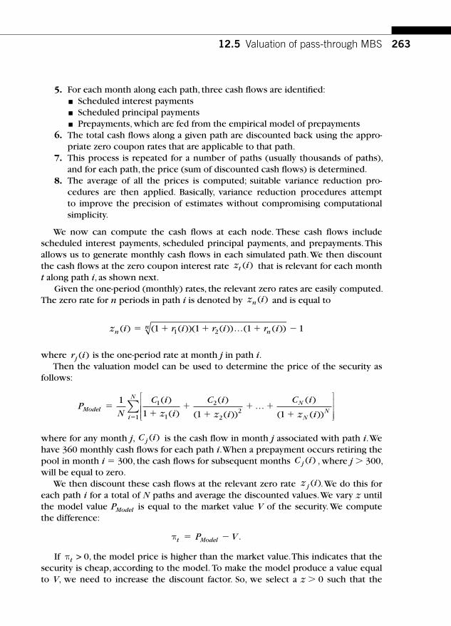
263
5. For each month along each path, three cash fl ows are identifi ed: ■ Scheduled interest payments ■ Scheduled principal payments ■ Prepayments, which are fed from the empirical model of prepayments
6. The total cash fl ows along a given path are discounted back using the appro-priate zero coupon rates that are applicable to that path.
7. This process is repeated for a number of paths (usually thousands of paths), and for each path, the price (sum of discounted cash fl ows) is determined.
8. The average of all the prices is computed; suitable variance reduction pro-cedures are then applied. Basically, variance reduction procedures attempt to improve the precision of estimates without compromising computational simplicity.
We now can compute the cash fl ows at each node. These cash fl ows include scheduled interest payments, scheduled principal payments, and prepayments. This allows us to generate monthly cash fl ows in each simulated path. We then discount the cash fl ows at the zero coupon interest rate z it ( ) that is relevant for each month t along path i , as shown next.
Given the one-period (monthly) rates, the relevant zero rates are easily computed. The zero rate for n periods in path i is denoted by z in ( ) and is equal to
z i r i r i r in nn( ( ( ))( ( )) ( ))) (� � � � �1 1 1 11 2 …
where r ij ( ) is the one-period rate at month j in path i. Then the valuation model can be used to determine the price of the security as
follows:
PN
C i
z i
C i
z i
C i
z iModel
N
NN
��
��
� ��
1
1 1 11
1
2
22
( )
( )
( )
( ( ))
( )
( ( ))…
⎡
⎣
⎢⎢⎢⎢
⎤
⎦
⎥⎥⎥
∑i
N
�1
where for any month j, C ij ( ) is the cash fl ow in month j associated with path i. We have 360 monthly cash fl ows for each path i. When a prepayment occurs retiring the pool in month i � 300, the cash fl ows for subsequent months C ij ( ) , where j � 300, will be equal to zero.
We then discount these cash fl ows at the relevant zero rate z ij ( ) . We do this for each path i for a total of N paths and average the discounted values. We vary z until the model value PModel is equal to the market value V of the security. We compute the difference:
πt ModelP V� � .
If πt > 0 , the model price is higher than the market value. This indicates that the security is cheap, according to the model. To make the model produce a value equal to V, we need to increase the discount factor. So, we select a z � 0 such that the
12.5 Valuation of pass-through MBS

264 CHAPTER 12 Mortgage-backed securities
model produces a price equal to the market value. This factor z is referred to as the option-adjusted spread (OAS). A positive OAS indicates that the security is cheap. Conversely, if the OAS is negative, the security is rich. The next equation shows the manner in which the OAS is computed:
V PN
C i
z i z
C i
z i z
C i
z iModel
N
N
� �� �
�� �
� ��
1
1 1 11
1
2
22
( )
( )
( )
( )
( )
(( ) (…
)) �� z Ni
N
)
⎡
⎣
⎢⎢⎢
⎤
⎦
⎥⎥⎥
∑1
The OAS is used extensively in the industry for determining the relative values of mortgage-backed securities.
12.5.1 Empirical behavior of an OAS
The OAS is a guide to determine which securities are rich and which are cheap. If the market price of an MBS is 97 and the model price is 98, the OAS is positive. We say that the security is “cheap. ” This does not necessarily imply that we should buy it. It will be useful to compare the OAS with the history of OAS and then interpret the current OAS in light of current economic circumstances. In a similar manner, if the market price of an MBS is 97 and the model price is 95, the OAS is negative. We say that the security is “rich. ” It should be remembered that the concept of OAS is only as good as the term structure model and the prepayment model. This implies that different dealers could assign a different OAS to the same security. A situation like that does not typically arise for pass-through securities, but it can happen for more esoteric mortgage-related securities, which tend to be illiquid. Often the history of an OAS of a security is used to assess the relative value of that MBS. To illustrate this idea, consider Figure 12.8 , which plots the OAS of three mortgage-backed pass-through securities for the period December 2005 to October 2007.
Note that the OAS of the GNMA is smaller than that of a Fannie Mae 15-year pass-through, which is in turn smaller than a Fannie Mae 30-year pass-through as of December 2005. By the criteria developed earlier, we would regard GNMA to be expensive (as its OAS � 0) as of that date, but over time, GNMA became cheaper relative to the model used in producing the OAS. Then investors would look at the history of OAS to determine whether a particular pass-through is attractive as invest-ment or not.
12.6 REMICS REMICs are real estate mortgage investment conduits, introduced in the Tax Reform Act of 1986. Prior to the Tax Reform Act, CMOs were issued as debt obligations of the issuer; thus, such issues appeared in a balance sheet as a liability. REMICs, on the other hand, are a legal framework within which mortgage-backed securities are treated as asset sales for tax purposes.

265
REMICs can be structured in a senior-subordinated format. This allows for credit enhancements to mortgage-backed securities with multiple tranches. REMICs rep-resent an innovative way to redistribute the cash fl ows from a pool of mortgages or mortgage-backed securities to various investor classes. Recall that investors in mortgage-backed pass-through securities get a pro rata share of the cash fl ows of the security, including prepayments. REMICs, through careful structuring, can offer varying levels of protection against prepayment risk. The REMIC issuance is backed by pools of residential mortgages or mortgage-backed securities, such as GNMAs, which serve as the collateral. The collateral is guaranteed by the GNMA, the FNMA, or the FHLMC.
12.6.1 REMIC structure
REMIC securities tend to be rated AAA or Aaa by the rating agencies. The key to this high credit reputation is the basic requirement that the cash fl ows generated by the underlying mortgages or the agency securities are more than suffi cient to meet the obligations of all tranches, even under the most extreme prepayment assumptions.
12.6 Remics
�40
�30
�20
�10
0
10
20
OA
S (
bp)
Dec-05 Apr-06 Aug-06 Dec-06 Apr-07 Aug-07
FNMA 30-year FNMA 15-year GNMA 30-year
FIGURE 12.8
The OAS of a Pass-Through MBS, December 2005 – October 2007

266 CHAPTER 12 Mortgage-backed securities
Let’s review some of the characteristics of general CMO structures. The credit risk is minimized by having a credible third party (such as a federal agency or an AAA insur-ance company) guarantee the cash fl ows.
The amount of collateral is set such that even under the most pessimistic prepay-ment assumptions, the total value of the bonds issued will be less than the value of the collateral. The typical worst-case assumption requires that all premium mort-gages be immediately prepaid and all discount mortgages have zero prepayments. REMIC securities, in general, pay semiannual or quarterly payments, but the underly-ing collateral or mortgages make monthly payments. This means that there is some reinvestment of the cash fl ows from the underlying collateral. Typically, conser-vative assumptions about the reinvestment rates are made by the rating agencies. Sometimes the rates that the issuer can get on guaranteed investment contracts (GICs) are used as indicators of possible reinvestment rates. The REMIC securities are typically overcollateralized. The purpose of this overcollateralization is to create an insurance cushion that helps offset any cash-fl ow shortages that may result due to a fall in reinvestment income from the underlying monthly cash fl ows. The cash fl ows from the collateral are divided and allocated to several classes or tranches of bonds. There are usually two basic REMIC structures: (1) a sequential structure and (2) a planned amortization class (PAC) structure.
12.6.2 Sequential structure
A typical generic REMIC sequential structure has four tranches. Specifi c rules dic-tate how the cash fl ows (including prepayments) from the collateral are allocated to each tranche. The total cash payment to each tranche is also set ahead of time. The fi rst tranche is allotted a stated coupon. In addition to this coupon, the fi rst tranche will also be allotted any prepayments that are made. Until the fi rst tranche is fully retired, no payments are made to the other tranches, except that the second and third tranches will receive the predetermined coupon amounts. The prepayments are passed through to the second tranche only after the fi rst is fully retired. In this sense, each tranche successively receives prepayments as soon as its immediate predecessor is retired. The last (here the fourth) tranche is called the Z bond and receives no cash fl ows until all earlier tranches are fully retired. The face amount, however, accrues at the stated coupon. After all tranches have been retired, the Z bond receives the coupon on its current face amount plus all the prepayments. Trustees ensure that the remaining collateral is large enough at all times so that all tranches get their promised cash fl ows. Most of the CMOs are rated AAA by the usual rating agencies. To provide the AAA rating, these agencies require that the present value of zero prepayment cash fl ows from the collateral at a discount rate equal to the maximum coupon of the bond determines the maximum amount of bonds that will be issued. The difference between the required bond payments and the cash fl ow received from the collateral is called the residual and is retained by the issuer of REMICs.

267
12.6.3 Planned amortization class structure
In a PAC structure, the tranches are created to provide varying levels of protection from prepayment. In this structure, the collateral’s principal is divided into two cat-egories. The fi rst category is designated PAC bonds, and the second category is the companion group. The amortization schedule for the PAC bonds remains fi xed over a range of prepayment rates measured by a range of PSAs. The more stable amortiza-tion schedule of the PAC group is at the expense of the companion group. The struc-ture, therefore, allows for many PAC bonds with stable average lives. The companion bonds, on the other hand, have much less stable lives than otherwise similar sequen-tial bonds. PAC bonds, because of their more stable amortization schedules, tend to be priced tightly to respective Treasuries. By the same token, bonds in the compan-ion group are priced at much wider spreads relative to Treasuries.
REMICs can be set up for designing securities that can meet the special needs of various investor groups. REMICs have been issued with tranches that pay coupons at levels tied to the London Interbank Offered Rates (LIBOR). These fl oating-rate CMOs have been popular with commercial banks and foreign institutional investors. Another type of REMIC, known as the targeted amortization class (TAC) CMO, are very similar to PAC CMOs; they also enjoy a specifi ed redemption schedule backed by support tranches in the CMO structure. Unlike PACs, TACs have a longer average maturity when interest rates fall and the prepayments are slower than expected.
SUGGESTED READINGS AND REFERENCES Anatomy of prepayments: Citigroup prepayments model. Salomon Smith Barney, Fixed Income
Research, March 2004.
Buser , S. A. , Hendershott , P. H., & Sanders , A. B. ( 1990 ) . Determinants of the value of call options on default-free bonds . Journal of Business , 63 ( 1) , 533 – 550 .
Dunn , K. , & McConnell , J. ( 1981 ) . Valuation of GNMA mortgage-backed securities . Journal of Finance , 36 ( 3) , 599 – 616 .
Waldman , M. , Schwalb , A. , & Feignberg , A. K. ( 1993 ) . Prepayments of fi fteen-year mortgages . Journal of Fixed Income , 2 ( 4) , 37 – 44 .
Suggested readings and references

This page intentionally left blank

269
CHAPTER
Fixed Income Markets and Their DerivativesCopyright 2009 by Academic Press. Inc. All rights of reproduction in any form reserved.
13 CHAPTER SUMMARY This chapter describes indexed bond markets in various parts of the world. The following issues are explored in this chapter: What are Treasury infl ation-protected securities (TIPS)? How do TIPS ’ yields differ from those of nominal government secu-rities? What is break-even infl ation level (BEI)? What are the important contractual and tax provisions of TIPS? Are TIPS useful in generating forecasts of future infl ation? The chapter explains how TIPS are sensitive to real rates but relatively insensitive to infl ation risk. The role of TIPS in a broad portfolio is addressed by documenting their relatively low to negative correlation with key asset classes. The return performance of Lehman TIPS index is presented.
13.1 OVERVIEW OF INFLATION-INDEXED DEBT We noted in earlier chapters that Treasury securities epitomize risk-free securities. Though it is certainly true that nominal securities issued by the U.S. Treasury are liquid, default-free, and carry certain tax advantages (exemption from local and state taxes), they are still subject to the risk of infl ation. The United States began to sell indexed Treasury securities in January 1997. These securities have little infl ation risk, and they enjoy the same advantages of the nominal securities issued by the Treasury in the sense that they are default-free, have become recently reasonably more liquid, and are exempt from local and state taxes. These securities are known as Treasury infl ation-protected securities, or simply TIPS. The principal value of TIPS is indexed to the nonseasonally adjusted (NSA) U.S. city average of all items consumer price index for all urban consumers (CPI-U). Table 13.1 provides the recent prices and yields of TIPS in four maturity sectors. For comparison, we also provide the prices and yields of nominal Treasury securities in the same benchmark maturities in Table 13.2 .
Infl ation-linked debt: Treasury infl ation-protected securities

270 CHAPTER 13 Infl ation-linked debt: Treasury infl ation-protected securities
As is customary, the prices are quoted in 32 nds. Note that the yields of TIPS are much lower than the yields of nominal Treasury securities. This is due to the fact that the TIPS compensate investors for infl ation risk, whereas the nominal Treasury securities do not offer any such compensation for realized infl ation that did not con-form to the expected infl ation rate at the time they were issued. The spread at the fi ve-year benchmark is (3.56% � 1.25%) � 231 basis points. This is referred to as the break-even infl ation (BEI) in the fi ve-year maturity. The reasoning is based on the following economic intuition: If the actual infl ation rate is below the BEI, TIPS will underperform nominal debt, and vice versa. We explore this idea further later. The BEI in the 10-year maturity is 250 basis points.
The market for global infl ation-indexed debt issued by governments has grown over the past 10 years, as shown in Table 13.3 .
Notice that the share of the global infl ation-indexed debt grew from 2.57% in 1997 to 9.37% in 2007. The dollar value of this market is now estimated at over $1.25 trillion. The government is in a unique position to sell infl ation-indexed securi-ties. It is reasonable to suggest that no other institution can offer such securities with any credibility. The Treasury is currently auctioning TIPS in the 5-year, 10-year, and 20-year benchmark maturities. It is using the Dutch auction scheme (uniform-price auction) to sell these securities as explained in Chapter 3. To attract a broad spec-trum of investors, Treasury is also selling infl ation bonds, or so-called I-bonds, which are now available in denominations of $50, $75, $100, $500, $1000, and $5000. Their earnings are indexed to infl ation, just as TIPS are, and they are exempt from local and
Table 13.1 TIPS Quotes as of July 23, 2008
Benchmark Coupon Maturity Price Yield
5-year 0.625% 04/15/2013 97 –04 1.25%
10-year 1.375% 07/15/2018 96 –02 1.81%
20-year 1.750% 01/15/2028 92 –27 2.27%
30-year 3.375% 04/15/2032 121–13 2.21%
Source: Bloomberg.
Table 13.2 Nominal Treasury Benchmark Quotes as of July 23, 2008
Benchmark Coupon Maturity Price Yield
2-year 2.875% 06/30/2010 100–04 2.81%
5-year 3.375% 06/30/2013 99 –04� 3.56%
10-year 3.875% 05/15/2018 97 –20.5 4.17%
30-year 4.375% 02/15/2038 94 –20� 4.71%
Source: Bloomberg.

271
state taxes. Under some circumstances, when the I-bonds are used for paying tuition and fees at eligible postsecondary educational institutions, all the earnings can qual-ify for exemption from federal taxes as well. In the United Kingdom, 50-year indexed debts (gilts) have been offered to investors since 2005.
The design and the issuance of TIPS are a hallmark event in the history of U.S. Treasury markets. If the Treasury develops this market as a signifi cant borrowing mechanism, TIPS can serve as the ultimate benchmark for measuring the cost of bor-rowing in real terms. The total amount of TIPS relative to other government debt in the United States is shown in Table 13.4 .
The size of TIPS is around $0.5 trillion out of $4.6 trillion government debt. It has become nearly as important as the T-bond market, and it appears it will become
Table 13.3 Growth of Infl ation-Indexed Government Bond Markets, 1997 – 2007
Year Nominal Government Debt ($ Billions)
Indexed Government Debt ($ Billions)
Indexed Debt as a Percentage of Total Government Debt
1997 5500 145 2.57%
1998 6401 207 3.13%
1999 6499 247 3.66%
2000 6278 268 4.09%
2001 6404 274 4.10%
2002 7771 360 4.43%
2003 9420 480 4.85%
2004 11,004 680 5.82%
2005 10,563 820 7.20%
2006 11,351 1039 8.39%
2007 12,397 1282 9.37%
Source: State Street Global Advisors, June 3, 2008.
Table 13.4 TIPS in the Context of Overall Treasury Debt, June 2008 ($ Millions)
Type Debt Held by Public Intragovernmental Holdings Total
T-bills 1,055,697 4,760 1,060,457
T-notes 2,542,526 9,116 2,543,442
T-bonds 580,995 64 581,059
TIPS 497,355 113 497,355
Source: Monthly statement of public debt, June 2008, U.S. Treasury.
13.1 Overview of infl ation-indexed debt

272 CHAPTER 13 Infl ation-linked debt: Treasury infl ation-protected securities
an important segment of the Treasury debt. In this chapter, we present an overview of global indexed government bond markets and take up in detail the U.S. indexed bond market. Indexation is by no means a new idea. Indexing means that the cash fl ows of the bonds (such as coupons and principal payments) are tied to some underlying index. In the 1700s, debt contracts were tied to the price of silver. In the 1930s, many debt securities were indexed to gold prices in the United States. As the debt markets and the bank loan markets developed, however, much of the con-tracting has continued to be in nominal terms as opposed to being in indexed form. This is despite the fact that many economists have persuasively argued for the use of indexed debt contracts by the government. The interest in issuing and investing in indexed debt securities is obviously tied to the perception of the risk of infl ation. Certainly, as infl ation risks became signifi cant in some economies, indexation began to take hold. Tables 13.5 and 13.6 summarize the development of indexed debt mar-kets in the world.
Table 13.5 Current Issuers of Infl ation-Indexed Government Bonds
Country First Issue Date Index Used
Australia 1985 Consumer prices
Brazil 1991 General prices
Canada 1991 Consumer prices
Chile 1967 Consumer prices
Colombia 1995 Consumer prices
Czech Republic 1997 Consumer prices
Greece 1997 Consumer prices
Hungary 1995 Consumer prices
Iceland 1995 Consumer prices
Israel 1955 Consumer prices
Mexico 1996 Consumer prices
New Zealand 1995 Consumer prices
Poland 1992 Consumer prices
Sweden 1994 Consumer prices
Turkey 1997 Consumer prices
United Kingdom 1981 Consumer prices
United States 1997 Consumer prices
Source : “Gilts and the Gilt Market Review 1996/97, ” Bank of England, List of Current Issuers of Infl ation-Indexed Government Bonds, 1997.

273
Table 13.5 summarizes the countries that issue infl ation-indexed bonds, vividly demonstrating that many countries have experimented with the issuance of indexed bonds. Note that the underlying indices have not varied much: Most countries have used the consumer prices as the index, but some have used wholesale prices, gold prices, wage index, and the like. The infl ation-indexed bonds market has taken hold in many countries, including Australia, Canada, Israel, and the United Kingdom. As should be clear, the United States is a relatively late entry into this market. Many Latin American countries (and a few others) tended to issue indexed bonds when the rate of infl ation ran very high. Campbell and Shiller (1996) report the time of introduction of indexed bonds and the rate of infl ation at that time in Table 13.6 .
Note that with the exception of Australia and New Zealand, most of the other countries issued indexed bonds when the infl ation rates are high. Indexed bonds represent a large chunk of the Israel debt market and a small but signifi cant part of the U.K. gilt market. In the United States, Treasury has indicated that the indexed debt issues will be made in suffi cient amounts to make this market a liquid one. What might be the motivation for government to issue debt that is indexed to infl a-tion? What types of investors might prefer infl ation-indexed bonds as opposed to nominal bonds? We turn to these questions now.
13.2 ROLE OF INDEXED DEBT Friedman has argued that government is solely responsible for infl ation, which expropriates the capital of investors in the Treasury securities. By offering infl ation-indexed securities, government will protect the welfare of investors who lent money to the government in the fi rst place. Moreover, by offering infl ation-indexed bonds, government gives itself a strong incentive to pursue anti-infl ationary policies. This incentive can also be encouraged by forcing the issuance of nominal securities in
Table 13.6 Timing of Introduction of Indexed Bonds by Country
Country Year of Introduction Rate of Infl ation at Introduction
Mexico 1989 114.80%
Argentina 1972 34.80%
Brazil 1964 69.20%
Chile 1966 22.20%
Israel 1955 12.30%
Australia 1985 4.50%
New Zealand 1977 2.80%
Source: Campbell and Shiller (1996).
13.2 Role of indexed debt

274 CHAPTER 13 Infl ation-linked debt: Treasury infl ation-protected securities
the shorter end of the yield curve. This obliges the Treasury to refi nance every time the short-term debt matures. Unless the infl ation rate is kept low, such refi nancing costs can be potentially high. The basic idea behind these arguments is the follow-ing: Either short-term nominal debt (requiring frequent refi nancing) or longer-term infl ation-indexed bonds will reduce the government’s incentive to infl ate. One might argue that of these two approaches, infl ation-indexed bond issuance provides a more cost-effective approach in the sense that we substitute by the one-time issu-ance cost of indexed bonds the multiple issuances associated with short-term debt and frequent refi nancing. Any infl ationary adjustment simply increases the principal of the indexed security and is thus a forced savings rather than an outright cash payout. Thus, the issuance of infl ation-indexed bonds simultaneously eliminates the moral hazard problem associated with the issuance of a long-term nominal debt and reduces the need to roll over and refund short-term nominal debt.
Others have argued that indexed securities may provide a useful function in pro-viding information about future expected infl ation rates. This can be extremely helpful to monetary authorities. Though this is true in principle, it is a good deal more complicated to extract the market’s expectations of infl ation rates using the prices of TIPS and other nominal Treasury securities. There are several reasons for this. First, most indexed bonds have lags in indexing. Such lags are necessary because the CPI numbers have to be compiled and distributed before the coupons and accrued interest of TIPS can be computed. (We show through several examples how this is done later in this chapter.) The presence of such lags limits the useful-ness of TIPS as a forecaster of expected infl ation rates.
Second, the tax treatment of TIPS will defi nitely infl uence the pricing and yields of TIPS. How the taxes affect yields and how they interact with real and nominal yields is still an unresolved question. Third, investors will typically require a risk premium associated with the infl ation risk. This risk premium has to be estimated and the manner in which it affects the expected infl ation rate has to be determined. This is a diffi cult task as well. Finally, there is an issue as to the differences in the liquidity of the nominal and TIPS market in any given maturity sector. For example, say that we are interested in examining the yields of 10-year TIPS with the yield of 10-year nomi-nal Treasury security. The liquidity of the 10-year nominal T-note is much higher than the 10-year TIP, and this can make the task of inferring infl ationary expectations that much more diffi cult. These problems notwithstanding, however, TIPS can potentially improve our understanding of expected infl ation rates in the economy once they become a signifi cant part of the government’s borrowing strategy.
The Treasury has also argued that the issuance of indexed bonds might reduce the cost of public debt. The reasoning is as follows: By offering securities that are indexed to infl ation, the Treasury is able to attract investors who are very averse to infl ation risk. Such investors will be willing to pay a higher price to buy securities that are default-free and that are indexed to infl ation. From the perspective of investors, infl ation-indexed bonds could prove to be attractive as well. For example, families that are saving for retirement or college might want to buy infl ation-indexed bonds because their expenses are expected to increase with infl ation. Likewise, institutions such as pension

275
funds and insurance companies that might have liabilities highly correlated with infl a-tion rate could want to include a signifi cant amount of infl ation-indexed bonds in their assets. Pension funds, which manage assets on behalf of defi ned-benefi ts plans, could be a particularly important class of investors who might benefi t from investing in indexed bonds. With the introduction of TIPS, fi rst-time investors have a reliable fi nancial security to hedge in the long term against the risks of infl ation.
The revenues and expenditures of the federal government are affected by the rate of infl ation. Tax revenues tend to be positively correlated with infl ation rate. This is not surprising, given that the taxes are based on the nominal income of citizens and corpo-rations. On the other hand, the expenditures of the federal government might not be so clearly correlated with the rate of infl ation. In fact, by borrowing in indexed securi-ties, both the revenues and the expenditures will be sensitive to the rate of infl ation.
In the short run, the market for TIPS is likely to be not very liquid due to the relatively small amounts that are currently outstanding in the market. This could imply wider bid-offer spreads until the market develops some depth. Some investors could also be averse to the idea of investing in bonds, which provide lower yields. It is also possible that the investors in TIPS do not trade actively; they could hold TIPS to dedicate the cash fl ows of TIPS to meet indexed liabilities. This might mean that the volume of trading in TIPS will be lower than that in nominal Treasury securities. This certainly appears to be the case in the United Kingdom, where both indexed gilts and nominal gilts are available.
One risk associated with investing in infl ation-indexed bonds is the risk that the index could undergo some future changes, which can adversely affect the investors who currently hold the security. Congress on occasion has instituted studies to over-haul the way CPI is calculated. There have been opinions that the CPI is overstated and that cost-of-living adjustments (COLA) are too generous. This represents a risk in much the same way that the tax treatment of municipal bonds has from time to time been questioned by Congress, leading to some uncertainty in municipal bond spreads.
13.3 DESIGN OF TIPS The design of TIPS is central to its potential success or failure. Roll (1996), in his insightful analysis of TIPS, identifi es the following key features in their design: (a) choice of index, (b) indexation lag, (c) maturity composition, (d) strippability, (e) tax treatment, and (f) cash-fl ow structure.
13.3.1 Choice of index
The Treasury’s design for TIPS was based on extensive consultations with the participants in the industry and is continuing to evolve based on the feedback that it has received. The key question in the design of TIPS is the choice of the index. Different countries have used different indexes. Various market participants within the same country might have preferences for different indexes. Several candidates exist in the market: the Consumer Price Index (CPI), wage indexes, indexes related to the costs of industrial
13.3 Design of TIPS

276 CHAPTER 13 Infl ation-linked debt: Treasury infl ation-protected securities
production, and indexes that are related to other important items in the household’s expenses. There are many important considerations in the choice of index. The integrity of the index must be beyond any doubt; the index should be maintained and updated in a scrupulous manner so that it refl ects the true cost of a representative consumption basket. It must be maintained by an agency that is independent of the government, to avoid any confl icts or “moral hazard ” problems whereby the index could be manipu-lated. In the United States, the Bureau of Labor Statistics reports the CPI, which is within the Department of Labor. The Bureau operates independently of the Department of the Treasury, providing it with independence over the calculation of the CPI. It might have been better if a nongovernmental agency were vested with the responsibility for the maintenance and upkeep of the index. The danger that investors might face in the choice of the index is the possibility that the index composition and the method of its calculation might change in the future in a way that adversely affects them.
The CPI (NSA) is the nonseasonally adjusted U.S. city average of all items on the consumer price index for all urban consumers. It is published monthly by the Bureau of Labor Statistics. The CPI measures the average change in prices over time in a fi xed market basket of goods and services, including food, clothing, shelter, fuels, transportation, medical services, and drugs. The weights used in the CPI refl ect their importance in the spending of urban households in the United States. The weights are updated periodically to refl ect any changes in the consumer expenditure pat-terns. The Treasury’s choice of the CPI-U is a good one because it is an index that is widely tracked by investors and dealers in the fi xed income markets. Roll (1996) suggests that other indexes tied to college tuition expenses or medical care expenses might be attractive to investors and can be politically attractive as well. The retail price index is used in the gilts market in the United Kingdom, and an index of gen-eral price level is used in Brazil. French government agencies have used indexes that are tied to the price of electricity, gas prices, coal prices, and the cost of rail travel. The behavior of CPI (NSA) over the period 1998 –2008 is shown in Table 13.7 .
Note that the infl ation as measured by the year-on-year change in CPI (NSA) in Table 13.7 shows some range: It reached a low of �1% during 2003 –2004 and a high of 6.4% during 2004 –2005. This evidence is indicative that the infl ation risk is rather signifi cant.
13.3.2 Indexation lag
If the indexed bond is perfectly indexed so that its payoffs refl ect at every instant the prevailing infl ation rate, such a bond will carry no risk at all with respect to the infl ation factor. Practical considerations, however, dictate that the indexed bonds will never be perfectly indexed. With the existing technology it is nearly impossible to adjust the cou-pon payment to refl ect the infl ation rate up to the last minute. This is due to the fact that the infl ation numbers have to be computed by the Bureau of Labor Statistics, and the process takes time. Thus, there is an unavoidable delay between the time the infl a-tion is measured and the time the cash fl ows are indexed to the measured infl ation rate.
This makes the indexed bond have some residual exposure to the infl ation risk. For example, an investor in month t knows that the indexing for the principal at

277
month t � 1 will not refl ect the current infl ation rate. This lag in indexing is prob-ably a more serious issue for short-term indexed securities when the volatility associ-ated with the infl ation risk is very high.
13.3.3 Maturity composition of TIPS
The U.S. Treasury has auctioned TIPS in 5-, 10-, and 20-year maturity sectors. The deci-sion to issue TIPS in the long-term maturity sectors is a very strong credible signal by the Treasury that it intends to keep the infl ation rate low. In addition to issuing TIPS in long maturity sectors, the Treasury also has allowed stripping of securities, which implies that long-dated strips that are indexed to infl ation will be available to investors. In the Canadian Treasury bond market, already infl ation-indexed bonds have been stripped. Now indexed strips have maturities ranging from a few months to more than 25 years. Such index-linked zeroes offering “real returns ” may be quite valuable to institutions that have indexed liabilities with long maturities. The decision to offer TIPS in a broad maturity spectrum will clearly improve the TIPS products that will be offered by the dealers. In TIPS, under normal infl ationary conditions, the nature of infl ation indexing“ backloads ” the cash fl ows. With longer maturities, this effect will be even stronger.
13.3.4 Strippability of TIPS
The Department of the Treasury has allowed the TIPS to be stripped. Because of the nature of indexing, which we discussed earlier, the strips were not fungible. As of
Table 13.7 Infl ation Experience, 1998 – 2008
Year CPI NSA CPI Year-on-Year Growth
1/15/1998 161.6 —
1/15/1999 164.0 1.5%
1/15/2000 168.3 2.6%
1/15/2001 174.1 3.4%
1/15/2002 177.6 2.0%
1/15/2003 181.3 2.1%
1/15/2004 179.4 � 1.0%
1/15/2005 191.0 6.4%
1/15/2006 198.4 3.9%
1/15/2007 201.7 1.6%
1/15/2008 209.5 3.9%
Source: Bureau of Labor Statistics, United States.
13.3 Design of TIPS

278 CHAPTER 13 Infl ation-linked debt: Treasury infl ation-protected securities
March 1999, however, the Treasury has announced certain changes that will allow for all the interest-only strips from Treasury infl ation-indexed securities with the same maturity date to be interchangeable (i.e., fungible). This is likely to promote liquid markets for stripped interest-only infl ation-indexed securities and could potentially increase the overall demand for the underlying TIPS. Note that investors can now buy long-dated real strips to hedge against infl ation. This should prove very attrac-tive to tax-sheltered retirement accounts such as IRAs and Keogh plans as well as to pension funds and insurance companies. These strips can be particularly useful in the annuities market to fund retirement benefi ts that are indexed to infl ation.
13.3.5 Tax treatment
Taxation of infl ation-indexed bonds poses a special issue: Should the appreciation in the principal amount due to infl ation and the resulting increase in coupon be taxed? The U.S. Treasury says they must be taxed. In fact, the periodic adjustments to the principal are to be treated as current income for tax purposes. This produces a “phantom income ” that is subject to taxation. At high enough infl ation rates, tax-able investors may experience negative cash fl ows from TIPS. This is a serious disad-vantage associated with investing in TIPS. In sharp contrast to the tax treatment in the United States, the capital gains accruing due to infl ation in index-linked gilts in the United Kingdom are exempt from taxation. For a taxable investor, this can be an advantage. The tax treatment accorded to TIPS in the United States is much like the tax treatment accorded to Treasury strips from nominal Treasury securities. In the case of strips, the investor must recognize a periodic taxable income, and this pro-duces a negative cash fl ow as well. There is a large clientele for strips (tax-deferred vehicles, such as the IRA and pension funds), and by the same reasoning, there will be a clientele for TIPS as well. Roll (1996) argues that taxing infl ation accruals may, in fact, be necessary to improve the liquidity of the TIPS market. Absent taxes on infl ation accruals, TIPS will trade at very low yields, and tax-exempt institutions will prefer nominal securities, which are likely to have higher pre-tax yields. Since tax-exempt institutions represent a signifi cant pool of investment capital, this will lead to an illiquid market for TIPS. Though this observation is correct, the bulk of the index-linked gilts in the United Kingdom are held by pension funds! The Bank of England reported in one study that the pension funds and insurance companies in the United Kingdom account for nearly 80% of the investment in the indexed-gilt market. In part, this incentive may be tied to the extent to which these pension funds are required to fully fund their indexed liabilities.
13.4 CASH-FLOW STRUCTURE There are varying cash-fl ow structures, beginning with a simple zero coupon structure to the U.S. TIPS structure, which is based on the Canadian infl ation-protected bonds. Here we briefl y outline the various structures and review their relative merits. To simplify

279
presentation, we will think of CPI as the index used in the cash-fl ow structure, although any index can be used in the following described structures. Let CPIt be the level of the index at date t, and let CPIT be the level of the index on the maturity date T.
13.4.1 Indexed zero coupon structure
An indexed zero coupon structure will pay at maturity date the amount equal to
100 �CPI
CPIT
t
.
This structure is the simplest and perhaps the most elementary unit of a real bond. As we saw earlier, stripping produces a security of this type except that the indexation lags will make the strip from TIP different from the pure zero coupon structure that we described previously. Note that the zero coupon structure pre sentsno reinvestment risk and presents the best protection from the risk of infl ation. Such countries as Canada, the United States, and Sweden have indexed zeroes, either through stripping or by outright issuance. From the perspective of forecasting, expected infl ation rates as well as the zero coupon structure are probably the best. Pension funds and insurance companies should fi nd this ideal in putting together indexed annuities without the risk of reinvestment. Unfortunately, the tax treatment in many countries would generate negative cash fl ows to taxable investors who must recognize the accrual of interest as well as infl ation in this structure. This could be one reason that we do not see this structure widely used in indexed bond markets.
13.4.2 Principal-indexed structure
This is the structure used by Canada and the United States. On coupon date s, the TIPS in the United States pay the amount
100 � �CPI
CPIT
t
At-issue-coupon rate.
At maturity, the payments from TIP will be
MaxCPI
CPIT
t
100 100, .�⎡
⎣⎢⎢
⎤
⎦⎥⎥
Note that the U.S. TIPS provide the investor with a put option at maturity that allows them to put the bond back to the Treasury at par, even if at maturity CPIT � CPIt . The presence of an embedded put option is obvious once we write the payoff at maturity as
100 0 100 100� � � �CPI
CPIMax
CPI
CPIT
t
T
t
,⎡
⎣⎢⎢
⎤
⎦⎥⎥ .
13.4 Cash-fl ow structure

280 CHAPTER 13 Infl ation-linked debt: Treasury infl ation-protected securities
13.4.3 Interest-indexed structure
On coupon date s, the interest-indexed real bond will pay the amount
100 1� � � �At-issue-coupon rate 100 .CPI
CPIT
t
⎡
⎣⎢⎢
⎤
⎦⎥⎥
Basically, the coupon payment has the standard at-issue coupon rate determined in the auction, plus the realized rate of infl ation.
13.5 REAL YIELDS, NOMINAL YIELDS, AND BREAK-EVEN INFLATION
To understand the differences between TIPS and nominal Treasury securities, we need to examine the relationship between nominal and real yields. To simplify mat-ters, let’s examine the relationship between the yields of a nominal zero coupon bond (say, a strip from nominal Treasury security) and a real zero coupon bond (such as a strip from a TIP).
Let the price of a nominal zero at time t paying a dollar at time t � 1 be $ pN. Then the nominal return i on this zero can be defi ned as $(1 � i) � pN � 1. Let’s assume that the consumer price index can be bought and sold. If CPIt is the consumer price index at time t and CPIt � 1 is the consumer price index at time t � 1, the (uncertain) rate of infl ation between these two dates denoted by π t can be found as follows:
CPI CPIt t t� � � �( )1 1π .
The expected rate of infl ation is then
EE CPI
CPItt
t
π[ ]( )
� ��1 1.
(13.1)
The real return on the nominal zero coupon bond is uncertain. The nominal zero pays at date t � 1 a real amount (in units of the consumer price index) of
1
1CPIt�
.
The real return on the nominal bond depends on the future consumer price index and is, therefore, uncertain. Hence, the real return on the nominal zero denoted by RN is found by comparing the real investment at date t with the real cash fl ow at date t � 1, as shown in Table 13.8 .
The real rate of return on the nominal bond is then defi ned as
p
CPIR
CPIN
tN
t
� � ��
( )11
1

281
or we can write the real return on the nominal zero as follows:
1 11
1
� � � ��
�
R
CPI
CPI
pi
CPI
CPIN
t
t
N
t
t
( ) . (13.2)
Writing this in terms of expected returns, we get
1 11
� � ��
E R i ECPI
CPINt
t
[ ]⎡
⎣⎢⎢
⎤
⎦⎥⎥( ) . (13.3)
We now consider a real zero coupon bond. Let its nominal price (in dollars) at time t be $ pR . At time t � 1, this bond will pay the index ratio of
CPI
CPIt
t
�1
to the holder. Then the real return RR on this real zero is certain because we know at time t that this zero will pay
#1
CPIt
units of the CPI at date t � 1. This certain real rate of return can be found as before by comparing the real investment at date t with the real cash fl ow at date t � 1, as shown in Table 13.9 .
The real rate of return on the real bond is then defi ned as
p
CPIR
CPIp
RR
tR
tR
R
� � � ��
( )11 1
1⇒ . (13.4)
Since the real rate of return on the nominal bond is uncertain, we will demand a risk premium for holding that bond. This is because the actual infl ation rate could differ from the expected rate of infl ation. This difference is referred to as the infl a-tion risk premium. Requiring that the nominal zero carries an infl ation risk pre-mium of y , we may write the expected real rate on the nominal bond as follows:
( ) ( ) ( ).1 1 1� � � �E R R yN R( ) (13.5)
Table 13.8 Real Return on a Nominal Zero
Transaction at Date t
Real Investment at Date t
Real Cash Flow at Date t � 1
Buy a nominal zero
pCPI
N
t
1
1CPIt �
13.5 Real yields, nominal yields, and break-even infl ation

282 CHAPTER 13 Infl ation-linked debt: Treasury infl ation-protected securities
For us to express the nominal yield in terms of expected infl ation rate, we use equations (13.1) and (13.3) in equation (13.5) to get
( ) ( ) ( ).11
11 1�
�� � �i E R y
tRπ
⎡
⎣⎢⎢
⎤
⎦⎥⎥
Unfortunately, we can show (by virtue of Jensen’s inequality) that
ECPI
CPIE
Et
t t t�
��
��1
1
1
1
1
⎡
⎣⎢⎢
⎤
⎦⎥⎥
⎡
⎣⎢⎢
⎤
⎦⎥⎥π π[ ]
.
Let’s write
EE xt t
1
1
1
1 1��
� �π π
⎡
⎣⎢⎢
⎤
⎦⎥⎥ ( ) ( )
where x is the convexity effect. The previous equation suggests that the relationship between nominal yields and real yields is affected by the infl ation risk premium and the expected infl ation rate. Under some simplifying assumptions, we can write the nominal yield as
1 1 1 1 1� � � � � �i R y E xR t[ ][ ][ ][ ]( ) .π
Ignoring the convexity effect for a moment and omitting the second-order effects, we can write the relationship between the nominal rates and the expected real rates as follows:
i R y ER t� � � ( ).π
This relationship explains why, the yields on TIPS shown in Table 13.1 are so much lower than the yields on nominal securities of similar maturities provided in Table 13.2. This difference will persist even on a duration-adjusted basis. This equation also explains why it is diffi cult to extract the information about the expected infl ation rates as the infl ation risk premium also enters the right side. As the expected infl ation
Table 13.9 Returns from Holding a Real (Indexed) Zero Coupon Bond
Transaction at Date t
Real Investment at Date t
Real Cash Flow at Date t � 1
Buy a real zero
pCPI
R
t
1CPIt

283
rates change, so does the infl ation risk premium. This is readily seen by noting that the changes in the nominal rates of interest arise from changes in the expected infl a-tion rates and changes in the infl ation risk premium.
Note that in our analysis we did not incorporate the effects of lags in indexing to infl ation. This is likely to cause the infl ation risk premium to go up. Although the delay in the U.S. market is two months in the gilts markets, the delay can be as high as eight months.
To give a better perspective on how the yields on TIPS have performed over time, Figure 13.1 plots over the period 1997 –1999 the yields on both 10-year nominal securities and 10-year infl ation protected securities.
Not surprisingly, the yields on nominal securities are much more volatile than the yields on TIPS. This is because much of the infl ation risk is already refl ected in the prin-cipal value of TIPS, whereas the nominal securities have a fi xed principal and coupon. The yields of TIPS also refl ect the poor liquidity of the market. DuPont and Sack (1999) report that 50% of the largest price changes in TIPS took place around auctions of TIPS. The liquidity of TIPS is lower than nominal treasury securities. As a consequence, inves-tors prefer the more liquid securities in periods of fi nancial distress. Note that during the second half of 1998 (Russian default, hedge funds crisis), nominal yield fell dra-matically, even though the yields of TIPS did not change by much. Finally, infl ationary expectations and risk premium play an important part in the behavior of yields.
13.6 CASH FLOWS, PRICES, YIELDS, AND RISKS OF TIPS Computing the cash fl ows from TIPS is much more complicated than computing the cash fl ows from nominal Treasury securities. A detailed treatment of this topic can be found in the Federal Register, published by the Department of the Treasury, dated February 6, 1997. This section is drawn heavily from the rules and regulations laid out in that Federal Register.
Interest on TIPS is paid on a semiannual basis. The Treasury issues TIPS with a fi xed coupon rate. This rate remains a constant throughout the life of the secu-rity. This coupon rate is applied to the principal value, which is indexed to the CPI as described earlier. On any coupon payment date, the dollar value of interest is obtained by multiplying the coupon rate by the infl ation-adjusted principal on the coupon payment date. The infl ation adjustment is done by multiplying the par amount of the bond by the relevant index ratio. The key variables in the calculation of index ratios as of any date t (which can be a coupon payment date) are the CPIt,which is the reference index number on date t, and the reference index number on the issue date 0, which we denote as CPI 0. When the dated date is different from the issue date, we use the index number as of the dated date instead of the index num-ber as of the issue date. Then the index ratio IRt is defi ned as follows:
IRCPI
CPItt�0
.
13.6 Cash fl ows, prices, yields, and risks of tips

284 CHAPTER 13 Infl ation-linked debt: Treasury infl ation-protected securities
Twelve-month CPIinflation rate
1997 1998 1999
Percentage points
Yield spread
1
2
3Inflation expectations1
Ten-year TIIS
Ten-year nominal securities6.5
5.5
4.5
3.5
Yield (percent)
FIGURE 13.1
Yields on Nominal and Indexed Treasury Securities and Indicators of Infl ation, 1997 –1999 Note: Yield data are based on most recently issued securities and extend through October 1999; yield spread is yield on 10-year nominal securities less yield on 10-year TIIS. Expectations data and CPI data extend into the third quarter. 1 Median expectation of CPI infl ation over the next 10 years among professional forecasters surveyed by the Federal Reserve Bank of Philadelphia. Source: Dominique DuPont and Brian Sack, “The Treasury Securities Market: Overview and Recent Developments,” Federal Reserve Bulletin , December 1999.

285
Note that the reference index number for the fi rst day of any calendar month is the CPI for the third preceding calendar month. For example, consider the fol-lowing hypothetical example. The reference CPI applicable to April 1, 1996, will be the CPI of January 1, 1996, of that year, which only gets reported in February 1996. This lag affects the effectiveness of TIPS against infl ation risk, as we will see later. The reference CPI for any other day of the month is then obtained by simple linear interpolation. For example, say that we are interested in fi guring out the index ratio for April 15 (which is the issue date of a TIP) of a year. Then
CPI CPI CPI CPIApril April May April15 1 1 114
30� � �⎡
⎣⎢⎤⎦⎥ .
Now CPIApril 1 is the nonseasonally adjusted CPI-U for January 1996 and is equal to 154.40 (from the Bureau of Labor Statistics). Likewise, CPIMay is the nonseasonally adjusted CPI-U for February 1996 and is equal to 154.90 (also from the Bureau of Labor Statistics). Combining these, we get
CPI April 15 154 1014
30154 90 154 40 154 3333� � � �. . . . .[ ]
Now we have the reference index number for the issue date as 154.3333. The index ratio for April 16 will then be computed simply as
IRCPI
CPItApril
April
�16
15
.
Note that we can now compute the CPIApril 16 as
CPI April 16 154 1015
30154 90 154 40 154 3500� � � �. . . . .[ ]
Therefore, the index ratio for April 16, 1996 is
IRCPI
CPItApril
April
� � �16
15
154 3500
154 33331 00011
.
.. .
This way, the index ratios can be computed for each day. Let’s examine in Example 13.1 how these calculations affected the coupon payments.
Example 13.1 A TIP was issued on April 15, 1996, with a coupon rate of 3.5%. The fi rst interest payment date for this TIP was October 15, 1996. The reference CPI number for the issue date of April 15, 1996, was 120.00. The reference CPI number for October 15, 1996, was l35.00. Then, for a par value of $1 million, what was the coupon income on October 15, 1996?
13.6 Cash fl ows, prices, yields, and risks of tips

286 CHAPTER 13 Infl ation-linked debt: Treasury infl ation-protected securities
Table 13.10 CPI Numbers for the Months Preceding July 1997
CPI-U(NSA) March 1997 160.00
CPI-U(NSA) April 1997 160.20
CPI-U(NSA) May 1997 160.10
The indexed principal was
1 000 000135120
1 125 000, , , , .� �
The coupon income was then
1 125 0000 035
219 687 50, ,
., . .� �
The accrued interest and the settlement price of TIPS can be computed in a manner similar to nominal Treasury securities. We illustrate the accrued interest calculations in Example 13.2.
Example 13.2 The Treasury issued an infl ation-indexed bond with a CUSIP number 9128272M3, with the following particulars: The issue date was February 6, 1997, and the dated date was January 15, 1997. The issue was reopened on April 15, 1997. The bond was to mature on January 15, 2007. The reference CPI number for the dated date stood at 158.43548. The coupon rate of the bond was 3.375%.
The Treasury published the following CPI numbers for the months that proceeded July 1997, as shown in Table 13.10 .
So, what is the accrued interest on this TIP as of July 2, 1997? To answer this question, we must fi rst compute the index ratios as in Example 13.1. Based on the CPI calculations, it is easy to compute the index ratios for the month of July 1997. We show the index ratios for the fi rst 10 days of July 1997 in Table 13.11 .
The previous coupon date was January 15, 1997, and the next coupon date was July 15, 1997. The accrued interest was simply
# days between 7/2/1997 and 1/15/1997# days between 1/15/19997 and 7/15/1997
� � �3 375
2100 1 01112
. %. .
The formula is identical to the way we compute the accrued interest for nominal Treasury securities except that we multiply the result by the index ratio as of the settlement date, which is 1.01112 for July 2, 1997. The resulting accrued interest is 1.58371. We obtain the index ratio for July 2, 1997, from Table 13.11 as 1.01112.

287
Table 13.11 Index Ratios, July 1 – 10, 1997
Day Calendar Day Ref. CPI Index Ratio
July 1, 1997 1 160.20000 1.01114
July 2, 1997 2 160.19677 1.01112
July 3, 1997 3 160.19355 1.01110
July 4, 1997 4 160.19032 1.01108
July 5, 1997 5 160.18710 1.01106
July 6, 1997 6 160.18387 1.01104
July 7, 1997 7 160.18065 1.01101
July 8, 1997 8 160.17742 1.01099
July 9, 1997 9 160.17419 1.01097
July 10, 1997 10 160.17097 1.01095
Table 13.12 Details of the Example TIP
Dated date: 15 January 1999
Original issue date 15 January 1999
Additional issue date 15 July 1999
Maturity date 15 January 2009
Reference CPI on dated date 164
The prices and yields can also be computed in exactly the same manner as we did for nomi-nal Treasury securities, except that the invoice price will have to refl ect the index ratio level as of the settlement date. We illustrate these calculations next in Example 13.3.
Example 13.3 The U.S. Treasury issued a TIP with the particulars shown in Table 13.12 . For the settlement date of October 18, 1999, the clean (fl at) price of this bond was 97.953125. What was the yield of this indexed bond? What was its invoice price?
As in the previous example, it is necessary to compute the index ratios fi rst.
13.6 Cash fl ows, prices, yields, and risks of tips

288 CHAPTER 13 Infl ation-linked debt: Treasury infl ation-protected securities
Table 13.13 Correlation of TIPS Returns with Other Asset Classes, December 1997 –December 2007
TIPS Index (Lehman)
TIPS Index (Lehman) 100%
S &P 500 � 67%
U.S. Treasury Index (Lehman) 71%
Source: Lehman Brothers.
First we need to compile the CPI-U information for the months preceding October 1999. We can gather this information from the Bureau of Labor Statistics. The index ratio for the settlement date of October 18, 1999, stood at 1.0178. Based on that infor-mation, we must fi rst compute the accrued interest. Note that the previous coupon date is July 15, 1999, and the next coupon date is January 15, 2000. The accrued inter-est is based on the index ratio on the settlement date, which is 1.01780:
Accrued � � � � �95
184
3 875
2100 1 01780 1 018146
. %. . .
The settlement price can be computed by adding the accrued interest to the clean price and then multiplying the result by the index ratio. The fl at price must fi rst be multiplied by the index ratio, and to this we add the accrued interest to get the invoice price as shown:
Invoice Price � � � �[97.953125 1.01780] 1.018146 100.714836.
The yield of the TIP can be computed using the Excel yield function in exactly the same way as we did for nominal Treasury securities in Chapter 2.
13.7 INVESTOR’S PERSPECTIVE From the investor’s perspective, TIPS offer protection from unanticipated increases in infl ation by the process of indexation. This is a fairly important attribute. The price sensitivity of TIPS to infl ation rate is low due to the fact that coupons and prin-cipal automatically change to refl ect market infl ation. In addition, TIPS have a fairly low to negative correlation with stock market indexes, as shown in Table 13.13 . Hence they are very good candidates as an asset class for inclusion into a broad portfolio.
If the TIPS are perfectly indexed, they will carry no infl ation risk and, therefore, will have zero duration with respect to the infl ation rate. TIPS tend to carry lower coupons, and infl ation accruals to par value are realized only at maturity. These two factors tend to increase the duration of TIPS. TIPS and nominal bonds react the same

289
Table 13.14 Duration of TIPS and Nominal Bonds
Price Sensitivity to:
Coupon Maturity Infl ation Real Rate Nominal Rate
5-year TIP Nominal
3- 3/8 6 -3/8
1/15/2007 2/15/2007
� 0.001 3.932
4.10 3.91
1.10 3.90
10-year TIP Nominal
3 -3/8 4 -7/8
1/15/2012 2/15/2012
� 0.001 7.440
8.02 7.44
3.40 7.40
30-year TIP Nominal
3 -7/8 6 -1/8
4/15/2029 8/15/2030
� 0.018 13.306
17.10 13.45
5.40 13.30
Source: Brett Hammond, “ Understanding and Using Infl ation Bonds, ” Research Dialogue, TIAA-CREF Institute, No. 73, September 2002.
Table 13.15 TIPS Return and Risk, December 31, 1997 – December 31, 2007
Sector Average Return Standard Deviation
Lehman Global Indexed-Linked Debt (Hedged in US$)
7.02% 3.35%
Lehman U.S. TIPS 7.50% 4.76%
Lehman U.S. Aggregate 5.92% 3.76%
Lehman U.S. Treasury 5.83% 4.43%
Source: Lehman Brothers and State Street Global Advisors.
way with respect to changes in real rates: When real rates go up, both prices will fall, and vice versa. The modifi ed duration of TIPS and otherwise similar nominal bonds can show some important differences, as shown in Table 13.14 .
On the other hand, TIPS appreciate if there is an unanticipated increase in infl a-tion rate. Nominal bond prices will fall under those circumstances. This implies that surprises in expected infl ation, which result in higher than anticipated infl ation, will cause the yields on TIPS to fall and the yields on nominals to increase, result-ing in widening spreads. The transaction costs of buying and selling TIPS have fallen and the market liquidity has improved since their introduction in 1997. State Street Global Advisors report that the transaction costs of trading a $100 million position in TIPS fell from $200,000 in 2002 to $50,000 in 2006. 1
Finally, Table 13.15 provides historical return-risk performance of TIPS. Note that global infl ation-linked bonds and TIPS have provided superior returns
compared to Lehman aggregate, although TIPS have subjected investors to slightly
1James Mauro and Jim Hopkins, Sr., “Global Linkers versus U.S. TIPs,” Global Fixed Income, State Street Global Advisors, fi xed income essay and presentation, June 3, 2008.
13.7 Investor’s perspective
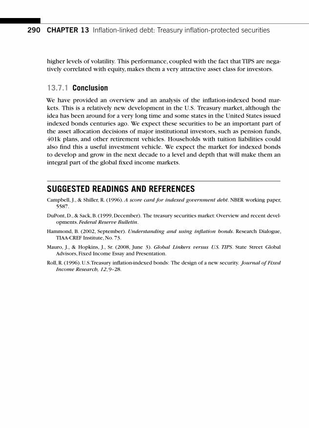
290 CHAPTER 13 Infl ation-linked debt: Treasury infl ation-protected securities
higher levels of volatility. This performance, coupled with the fact that TIPS are nega-tively correlated with equity, makes them a very attractive asset class for investors.
13.7.1 Conclusion
We have provided an overview and an analysis of the infl ation-indexed bond mar-kets. This is a relatively new development in the U.S. Treasury market, although the idea has been around for a very long time and some states in the United States issued indexed bonds centuries ago. We expect these securities to be an important part of the asset allocation decisions of major institutional investors, such as pension funds, 401k plans, and other retirement vehicles. Households with tuition liabilities could also fi nd this a useful investment vehicle. We expect the market for indexed bonds to develop and grow in the next decade to a level and depth that will make them an integral part of the global fi xed income markets.
SUGGESTED READINGS AND REFERENCES Campbell, J., & Shiller, R. (1996). A score card for indexed government debt. NBER working paper,
5587.
DuPont , D. , & Sack , B. ( 1999, December ) . The treasury securities market: Overview and recent devel-opments . Federal Reserve Bulletin .
Hammond, B. (2002, September). Understanding and using infl ation bonds. Research Dialogue, TIAA-CREF Institute, No. 73.
Mauro, J., & Hopkins, J., Sr. (2008, June 3). Global Linkers versus U.S. TIPS. State Street Global Advisors, Fixed Income Essay and Presentation.
Roll , R. ( 1996) . U.S. Treasury infl ation-indexed bonds: The design of a new security . Journal of Fixed Income Research , 12 , 9 – 28 .

Fixed income derivatives 4
PART

This page intentionally left blank

293
CHAPTER
Fixed Income Markets and Their DerivativesCopyright 2009 by Academic Press. Inc. All rights of reproduction in any form reserved.
CHAPTER SUMMARY This chapter describes two important derivatives in the overnight money market segment of fi xed income markets. They are the Fed funds futures contracts and the overnight index swaps (OIS). These derivatives are used extensively by the market to try to anticipate the actions of the Fed and for risk management purposes. In this chapter we describe these contracts and develop simple valuation framework for OIS contracts.
14.1 OVERVIEW Overnight lending and borrowing are important parts of fi nancial markets. We saw in Chapter 5 how participants in fi xed income markets use repo markets for funding purposes on an overnight basis. In addition, the central bank uses repo transactions to implement some of its monetary policy goals, as exemplifi ed in the repo auctions discussed in Chapter 5. Banks fund themselves in overnight markets in interbank markets via overnight LIBOR transactions —another important index in money mar-kets. Reserve requirements are managed through the Fed funds market, which is also done on an overnight basis.
All these activities produce inherent risks. A dealer who has lent cash in the term repo market but funded himself in overnight repo markets faces the risk that over-night rates could escalate. A bank that is funding itself in the term markets by accept-ing term deposits may be exposed to the risk that the term funding rates could decline in the future. Over the last two decades two important derivatives markets have emerged to manage such risks. They are the Fed funds futures markets and the overnight index swap (OIS) market. They form the subject matter of this chapter.
Derivatives on overnight interest rates 14

294 CHAPTER 14 Derivatives on overnight interest rates
14.2 FED FUNDS FUTURES CONTRACTS The settlement prices of Fed funds futures as of July 11, 2008, were quoted as shown in Table 14.1 . Note that contracts extend on monthly intervals out to two full years.
The underlying asset to the Fed funds futures contract is the 30-day Fed funds rate. Let’s look at the contract specifi cation to better understand the nature of futures prices (see Table 14.2 ).
Table 14.1 Fed Funds Futures Prices, July 11, 2008
Implied Target Rate
Maturity Settlement Price 100 Minus Price
August 2008 97.975 2.025
September 2008 97.925 2.075
October 2008 97.865 2.135
November 2008 97.770 2.230
December 2008 97.740 2.260
January 2009 97.685 2.315
February 2009 97.575 2.425
March 2009 97.535 2.465
April 2009 97.490 2.510
May 2009 97.385 2.615
June 2009 97.345 2.655
July 2009 97.245 2.755
August 2009 97.145 2.855
September 2009 97.055 2.945
October 2009 97.055 2.945
November 2009 97.055 2.945
December 2009 97.055 2.945
January 2010 97.055 2.945
February 2010 97.055 2.945
March 2010 97.055 2.945
April 2010 97.055 2.945
May 2010 97.055 2.945
June 2010 97.055 2.945

295
The Fed funds futures contract is a cash-settled contract. The futures settlement price is computed as 100 minus the monthly arithmetic average of the daily effect-ive Fed funds rates. The trading desk of the Federal Reserve Bank of New York reports these rates. One basis point in a Fed funds futures contract is worth $41.67, as shown here:
$ ,000, $5 0001
100
1
100
30
36041 67� � � � .
Much of the liquidity in this market is concentrated on near-maturity contracts.
14.2.1 Recovering market expectations of future actions by the FOMC
Market participants use Fed funds futures to predict what the future target Fed funds rates might be. Suppose that the futures prices for a June 20 xx contract during the delivery month were as shown in Table 14.3 .
Table 14.3 records the effective Fed funds rates for one month. Note that the rates that prevail on Fridays are applied to the weekend as well. As of the last day of the month, the average effective Fed funds rate is 2.04367. This is rounded to 2.0436. Based on this amount, the futures settlement price is determined as 100 � 2.0436 � 97.9564.
14.2 Fed funds futures contracts
Table 14.2 Fed Funds Futures Specifi cations
Contract size $5 million
Tick size $20.835 per 1/2 of 1 basis point (1/2 of 1/100 of 1% of $5 million on a 30-day basis rounded up to the nearest cent)
Price quote 100 minus the average daily Fed funds overnight rate for the delivery month (e.g., a 7.25% rate equals 92.75)
Contract months First 24 calendar months
Last trading day Last business day of the delivery month; trading in expiring contracts closes at 2:00 p.m., Chicago time, on the last trading day
Settlement The contract is cash settled against the average daily Fed funds overnight rate, rounded to the nearest 1/10 of one basis point, for the delivery month; the daily Fed funds overnight rate is calculated and reported by the Federal Reserve Bank of New York
Trading hours Open auction: 7:20 a.m. – 2:00 pm, Central Time, Monday – Friday Electronic: 5:30 p.m. – 4:00 p.m., Central Time, Sunday – Friday
Ticker symbols Open auction: FF Electronic: ZQ

296 CHAPTER 14 Derivatives on overnight interest rates
This procedure suffers from a number of shortcomings: First, Fed funds futures contracts settle to the average of the relevant month’s effective overnight Fed funds rate. This is quite distinct from settlement to a rate on any specifi c day. If the goal is to form expectations about the target rate on a specifi c date, the aver-aging process in the settlement will introduce an error and must be accounted for. Second, futures contracts are based on the effective Fed funds rate. We saw in Chapter 3 that the target rate and the effective Fed funds rates are typically well within a few basis points of each other, but at times the difference between the effective Fed funds rate and the Fed’s target can be rather large. In addition, futures contracts are subject to daily marking to market, which may produce daily cash in fl ows and out fl ows. In this sense, we are not dealing with a forward contract, which has no cash fl ows until maturity. All these features must be taken into account in extracting the expectations from Fed funds futures prices. It is also important that the past average of effective Fed funds rate is removed from the quoted futures price in order to get a better idea of the expectations of effective Fed funds rate implied by the futures price.
Table 14.3 Effective Fed Funds Rates (Hypothetical)
Day of Month Effective Fed Funds Rate
Day of Month Effective Fed Funds Rate
1 (Mon) 2.02 16 (Tue) 2.05
2 (Tue) 2.03 17 (Wed) 2.07
3 (Wed) 2.06 18 (Thurs) 2.04
4 (Thurs) 2.04 19 (Fri) 2.05
5 (Fri) 2.02 20 (Sat) 2.05
6 (Sat) 2.02 21 (Sun) 2.05
7 (Sun) 2.02 22 (Mon) 2.06
8 (Mon) 2.04 23 (Tue) 2.06
9 (Tue) 2.05 24 (Wed) 2.07
10 (Wed) 2.03 25 (Thurs) 2.05
11 (Thurs) 2.04 26 (Fri) 2.05
12 (Fri) 2.04 27 (Sat) 2.05
13 (Sat) 2.04 28 (Sun) 2.05
14 (Sun) 2.04 29 (Mon) 2.04
15 (Mon) 2.05 30 (Tue) 2.03

297
14.3 OVERNIGHT INDEX SWAPS (OIS) An overnight indexed swap (OIS) is a swap in which one party agrees to pay fi xed and the other party agrees to pay a fl oating interest rate that is tied explicitly to a published index of a daily overnight rate benchmark such as the overnight Fed funds rate. The term of the OIS may range from a few days to two years or more. The swap also specifi es a notional principal. The two parties agree to exchange at maturity, on the agreed notional amount, the difference between interest accrued at the agreed fi xed rate and interest accrued through averaging of the fl oating benchmark rate.
OISs have become an important part of the fi xed income markets and an especially valuable tool in money markets. They are used extensively and are now available in all major countries. Table 14.4 shows OIS contracts in Europe, the United States, and the United Kingdom.
OIS contracts are particularly useful in hedging and taking positions in overnight interest rates. From an economic perspective, the receiver of a fi xed rate in an OIS has effectively lent out cash and is presumably borrowing in the overnight market or in the term market. Likewise, the payer of a fi xed rate in an OIS is effectively borrowing cash.
The principal is notional and is used for calculating the amount to be paid or received when the contract settles; there is no exchange of principal in OIS transactions.
14.3.1 Contract specifi cations
OIS swap exchanges a fi xed rate for a fl oating rate on a specifi ed future date, which is the swap’s maturity date.
Let rt be the fl oating rate on date t. In the case of OIS in the United States, this will pertain to the daily effective Fed funds rate. For Europe it will refer to EONIA. In the United Kingdom it will refer to SONIA, and so on. Let’s fi rst illustrate the averaging procedure by using an arithmetic average scheme. The fl oating payments denoted by r can be computed as follows:
r rd
tt
t
n
� �� 3601∑ . (14.1)
14.3 Overnight index swaps (OIS)
Table 14.4 OIS Swaps in the United States, Europe, and the United Kingdom
Country/Zones OIS Swap Underlying Index
United States Effective Fed funds rate, as calculated by the Federal Reserve Bank of New York
Europe Euro Overnight Index Average (EONIA), as calculated by the ECB
United Kingdom SONIA, as calculated by the British Bankers Association (BBA)

298 CHAPTER 14 Derivatives on overnight interest rates
In Equation 14.1, the notation dt is used to refer to the actual number of days for which the interest rate rt is applied. For example, if t happens to be a Friday, then dt will be three days. Normally, dt will be just one day. Also, n refers to the total number of days in the swap. Consider for example, a seven-day OIS in which the history of variable rates (such as effective Fed funds rates) followed the trajectory shown in Table 14.5 .
Applying Equation 14.1, we get the variable rate in the swap to be as follows.
1
73 00 3 01 3 02 3 3 00 3 00 3 01� � � � � � �. % . % . . % . % . %%[ ]
Note that the interest rate corresponding to Friday is given a weight of three days, whereas the others received weights of one day each. In most OIS markets such as the United States and in EONIA-based OIS contracts, a geometric averaging scheme is used for computing the fl oating payments, as illustrated here:
rn
r dt t
t t
t t
s
e
� ��
��
� �3601
3601
1 ⎛
⎝⎜⎜⎜
⎞
⎠⎟⎟⎟⎟
⎡
⎣⎢⎢
⎤
⎦⎥⎥∏ . (14.2)
In Equation 14.2, we denote by ts the start date of the swap and by te we denote the end date of the swap. The index used for the swap could be EONIA, which stands for Euro Overnight Index Average. It is a measure of the effective interest rate pre-vailing in the Euro interbank overnight market. It is calculated as a weighted average of the interest rates on unsecured overnight lending transactions denominated in Euros, as reported by a panel of contributing banks.
The structure of OIS contracts with geometric averaging as in Equation 14.2 implies that the fl oating leg of OIS actually exactly replicates the compounded return accrual of the fl oating index rate (such as EONIA) through the term of the swap. It should be noted that in the United States the fl oating rate is the weighted average for overnight transactions, as published by the central bank. In Europe it is the weighted average of interbank overnight or term transactions. OIS contracts have become extremely popular within a very short span of time.
Table 14.5 OIS Swap Example
Days of Week Effective Fed Funds Rate
Wednesday 3.00%
Thursday 3.01%
Friday 3.02%
Monday 3.00%
Tuesday 3.00%

299
14.4 VALUATION OF OIS Valuation of OIS contracts is fairly similar to the valuation of swaps with some modi-fi cations. First, we have to adjust for the fact that interest rates are being averaged in determining the fl oating payments. Second, there is only one terminal payment that is associated with OIS contracts. We begin with a simple example.
Example 14.1 Consider the overnight rates (EONIA) shown in Table 14.6 . X enters into a seven-day OIS contract, electing to receive a fl oating amount on a notional principal of 100 million Euros. X agrees to pay 3.00% annualized at the end of the swap. Calculate the variable rate that X will get and the net amount that she should pay or receive at the end of the swap.
14.4 Valuation of OIS
Table 14.6 Valuing OIS Swap
Days of Week EONIA
Wednesday 3.00%
Thursday 3.01%
Friday 3.02%
Monday 3.00%
Tuesday 3.00%
The variable rate will be computed by applying Equation 14.2, keeping in mind that Wednesday is the start date of the OIS contract and the contract ends after Tuesday, so we will include all the days in the table in computing the variable rate. Then, investor X’s compounded annualized return can be computed (by applying Equation 14.2) as follows:
r � �
� � ��
360
7
10 0300
3601
0 0301
3601
0 0302. . .⎛⎝⎜⎜⎜
⎞⎠⎟⎟⎟⎛⎝⎜⎜⎜
⎞⎠⎟⎟⎟
33
360
10 0300
3601
0 0300
360
⎛⎝⎜⎜⎜
⎞⎠⎟⎟⎟
⎛⎝⎜⎜⎜
⎞⎠⎟⎟⎟⎛⎝⎜⎜⎜
⎞⎠⎟⎟⎟� � �
. .11
⎡
⎣
⎢⎢⎢⎢⎢⎢
⎤
⎦
⎥⎥⎥⎥⎥⎥
This variable rate is 3.0106%. Her net payment at the end of the swap may be computed as follows:
100 100000 3 0106 3 007
360207 02� � � � �( . % . %) .
Note that as of the morning of the start date, investor X will not have knowledge of the rates shown in the table. But imagine the investor taking $1 and investing from the beginning of Wednesday until the end of Tuesday in a sequence of overnight
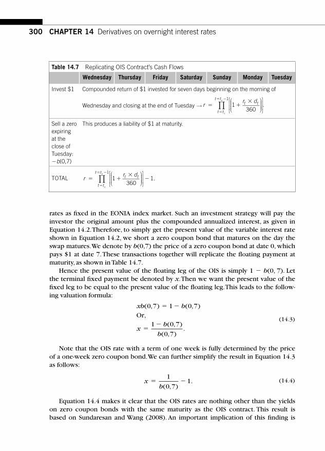
300 CHAPTER 14 Derivatives on overnight interest rates
rates as fi xed in the EONIA index market. Such an investment strategy will pay the investor the original amount plus the compounded annualized interest, as given in Equation 14.2. Therefore, to simply get the present value of the variable interest rate shown in Equation 14.2, we short a zero coupon bond that matures on the day the swap matures. We denote by b(0,7) the price of a zero coupon bond at date 0, which pays $1 at date 7. These transactions together will replicate the fl oating payment at maturity, as shown in Table 14.7 .
Hence the present value of the fl oating leg of the OIS is simply 1 � b(0, 7). Let the terminal fi xed payment be denoted by x. Then we want the present value of the fi xed leg to be equal to the present value of the fl oating leg. This leads to the follow-ing valuation formula:
xb b
xb
b
( , ) ( , )
,( , )
( , ).
0 7 1 0 7
1 0 7
0 7
� �
��
Or(14.3)
Note that the OIS rate with a term of one week is fully determined by the price of a one-week zero coupon bond. We can further simplify the result in Equation 14.3 as follows:
xb
� �1
0 71
( , ). (14.4)
Equation 14.4 makes it clear that the OIS rates are nothing other than the yields on zero coupon bonds with the same maturity as the OIS contract. This result is based on Sundaresan and Wang (2008). An important implication of this fi nding is
Table 14.7 Replicating OIS Contract’s Cash Flows
Wednesday Thursday Friday Saturday Sunday Monday Tuesday
Invest $1 Compounded return of $1 invested for seven days beginning on the morning of
Wednesday and closing at the end of Tuesday →
rr dt t
t t
t t
s
e
� ��
�
� �
1360
1 ⎛
⎝⎜⎜⎜
⎞
⎠⎟⎟⎟⎟
⎡
⎣⎢⎢
⎤
⎦⎥⎥∏ .
Sell a zero expiringat the close of Tuesday: � b (0,7)
This produces a liability of $1 at maturity.
TOTAL
rr dt t
t t
t t
s
e
� ��
��
� �
1360
11 ⎛
⎝⎜⎜⎜
⎞
⎠⎟⎟⎟⎟
⎡
⎣⎢⎢
⎤
⎦⎥⎥∏ .

301
that the OIS yields will have term premiums in them. Hence, they do not generally measure the expected average of the underlying policy rates.
Consider a bank that has received $100 million in one-year deposits. The bank has to pay the depositing customer the one-year deposit rates. The bank could enter into a one-year OIS transaction in which it receives fi xed and pays the average of the effective Fed funds rate. Through such a transaction, the bank has effectively funded its deposit at the overnight interest rates.
14.5 OIS SPREADS WITH OTHER MONEY MARKET YIELDS With the theory of valuing OIS rates in place, we can now examine the spreads between OIS rates and other money market rates. To provide context to this issue, we plot in Figure 14.1 the spreads of OIS relative to LIBOR, or more precisely, LIBOR minus the OIS rate.
Note that the LIBOR-to-OIS spread was very stable and only slightly deviated from a level of about 10 basis points or below until August 2007. The onset of the credit crisis of 2007 –2008 caused the LIBOR to increase dramatically over the OIS
14.5 OIS spreads with other money market yields
Date
01/0
1/07
02/0
1/07
03/0
1/07
04/0
1/07
05/0
1/07
06/0
1/07
07/0
1/07
08/0
1/07
09/0
1/07
10/0
1/07
11/0
1/07
12/0
1/07
02/0
1/08
03/0
1/08
04/0
1/08
05/0
1/08
01/0
1/08
�20
�10
0
10
20
30
40
50
60
70
80
90
100
110
Non-credit component
Default premium
LIBOR-OIS spread
Bas
is p
oint
s
FIGURE 14.1
LIBOR Minus OIS Rate, January 2007 – May 2008 Source: James McAndrews, Asani Sarkar, and Zhenyu Wang, “ The Effect of the Term Auction Facility on the London Inter-Bank Offered Rate, ” Staff Report No. 335, July 2008, Federal Reserve Bank of New York.

302 CHAPTER 14 Derivatives on overnight interest rates
rate. As we noted earlier, the OIS rate is simply the yield on a zero coupon bond. Since OIS contracts have no principal exchange, they are relatively free from default risk. Hence, as a fi rst approximation, we can regard the OIS rate as a risk-free rate in between two private counterparties in capital markets. This is in contrast to T-bill yields, which can be issued only by the U.S. Treasury and are subject to “safe haven ”premiums and hence are not an appropriate measure of risk-free rate from the per-spective of private borrowers. The behavior of the LIBOR/OIS spread suggests that there are two factors at work: First, the LIBOR market involves actual exchange of principal from one bank to another at maturity. In contrast, OIS contracts are on notional amounts with no exchange of principal at maturity. This introduces credit/default risk into LIBOR but not necessarily in OIS markets. Hence, at least part of the spread between LIBOR and OIS is attributable to this source of risk.
In addition, it could be argued that the LIBOR market is subject to inadequate participation by banks in a period of crisis: Banks might be concerned about the credit exposure of other banks and might simply not be willing to lend. This intro-duces an element of illiquidity. This factor must account for the remaining spreads between LIBOR and OIS. McAndrews, Sarkar, and Wang (2008) examine the extent to which the spreads can be decomposed into these two components and the effect that the central bank’s liquidity provision (through its term lending facilities) has had on lowering the overall spreads.
SUGGESTED READINGS AND REFERENCES EONIA Swap Index. The derivatives market reference rate for the Euro. The Financial Markets
Association.
Euro money markets study 2006 . European Central Bank, February 2007.
Kuttner , K. ( 2001) . Monetary policy surprises and interest rates: Evidence from the fed funds futures market . Journal of Monetary Economics , 47 ( 3) , 523 – 544 .
McAndrews, J., Sarkar, A., & Wang, Z. (2008, July). The effect of the term auction facility on the London inter-bank offered rate . Staff Report No. 335. Federal Reserve Bank of New York.
Overnight Index Swaps (2001, December). Credit Suisse First Boston.
Sundaresan, S., & Wang, Z. (2008). Overnight Index Swap valuation and LIBOR-OIS spreads. Draft, August 2008.

303
CHAPTER
CHAPTER SUMMARY This chapter introduces Eurodollar cash and futures markets. The manner in which LIBOR is determined by the British Bankers Association (BBA) is explained. The set-tlement of Eurodollar futures to LIBOR is described, and the procedure for extract-ing discount factors (zero prices) from Eurodollar futures is shown by an example. We show how Eurodollar futures prices can be used to value interest rate swaps. Hedging applications using Eurodollar futures are illustrated. Options on Eurodollar futures are used to construct caps, fl oors, and collars on LIBOR.
15.1 EURODOLLAR MARKETS AND LIBOR Eurodollars are bank deposits denominated in U.S. dollars but not subject to U.S. banking regulations. Typically they are located outside the United States. International Banking Facilities (IBFs) located in the United States can also conduct such transac-tions free of U.S. regulations. Eurodollar time deposits (TDs) are liabilities of IBFs and other banks located outside the United States. It is an interbank market in which participating banks borrow and lend with each other. LIBOR, the London Interbank Offered Rate, refl ects the rate at which the banks offer loans to their member banks. LIBID, the London Interbank Bid Rate, refl ects the rate at which the banks take loans from their member banks. The rates can vary from bank to bank, refl ecting their eco-nomic circumstances. The market’s liquidity is primarily in the short-term sector. For simplicity we will ignore the differences between LIBOR and LIBID and simply work with the term LIBOR throughout.
The LIBOR spot market ranges in maturities ranging from a few days to 10 years. The depth of the market is especially great in the three- and six-month maturity sectors.
Eurodollar futures contracts 15
Fixed Income Markets and Their DerivativesCopyright 2009 by Academic Press. Inc. All rights of reproduction in any form reserved.

304 CHAPTER 15 Eurodollar futures contracts
The market for Eurodollar deposits is among the largest fi nancial markets with many participating institutions. In fact, many other fi nancial markets, such as the swap markets, Eurodollar futures markets, and the commercial paper markets, to name just three, regard LIBOR as benchmarks in setting their relevant rates. These LIBOR benchmark rates are not based on any one bank’s LIBOR quote but based on a LIBOR fi xing process.
15.1.1 LIBOR fi xing
The British Bankers Association (BBA) determines the benchmark LIBOR by aver-aging the interbank borrowing rates of selected banks (members of the BBA panel) after eliminating outliers.
In each currency, a panel of banks is used to obtain quotes of LIBOR. The panels as of 2008 for U.S. dollar LIBOR determination are shown in Table 15.1 .
Note that there are 16 banks in the panel. The panel contributes rates to BBA; the rates are ranked, and only the rates in the middle quartiles are used in a simple arithmetic-averaging process to fi x LIBOR. Therefore LIBOR refl ects the average credit quality
Table 15.1 U.S. Dollar LIBOR Panel, July 2008
Bank of America
Bank of Tokyo-Mitsubishi UFJ Ltd.
Barclays Bank plc
Citibank NA
Credit Suisse
Deutsche Bank AG
HBOS
HSBC
JP Morgan Chase
Lloyds TSB Bank plc
Rabobank
Royal Bank of Canada
The Norinchukin Bank
The Royal Bank of Scotland Group
UBS AG
West LB AG
Source: British Bankers Association (BBA).
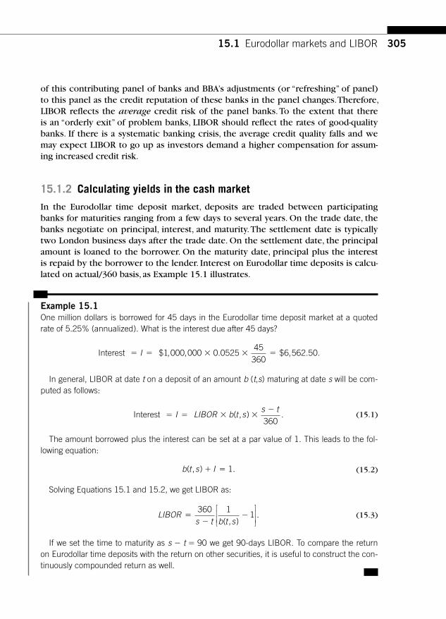
305
of this contributing panel of banks and BBA’s adjustments (or “ refreshing ” of panel) to this panel as the credit reputation of these banks in the panel changes. Therefore, LIBOR refl ects the average credit risk of the panel banks. To the extent that there is an “orderly exit ” of problem banks, LIBOR should refl ect the rates of good-quality banks. If there is a systematic banking crisis, the average credit quality falls and we may expect LIBOR to go up as investors demand a higher compensation for assum-ing increased credit risk.
15.1.2 Calculating yields in the cash market
In the Eurodollar time deposit market, deposits are traded between participating banks for maturities ranging from a few days to several years. On the trade date, the banks negotiate on principal, interest, and maturity. The settlement date is typically two London business days after the trade date. On the settlement date, the principal amount is loaned to the borrower. On the maturity date, principal plus the interest is repaid by the borrower to the lender. Interest on Eurodollar time deposits is calcu-lated on actual/360 basis, as Example 15.1 illustrates.
Example 15.1 One million dollars is borrowed for 45 days in the Eurodollar time deposit market at a quoted rate of 5.25% (annualized). What is the interest due after 45 days?
Interest � � � � �I $ , , . $ , . .1 000 000 0 052545
3606 562 50
In general, LIBOR at date t on a deposit of an amount b ( t , s) maturing at date s will be com-puted as follows:
Interest � � � ��
I LIBOR b t ss t
( , ) .360
(15.1)
The amount borrowed plus the interest can be set at a par value of 1. This leads to the fol-lowing equation:
b t s I( , ) .� � 1 (15.2)
Solving Equations 15.1 and 15.2, we get LIBOR as:
LIBORs t b t s
��
�360 1
1( , )
.⎡
⎣⎢⎢
⎤
⎦⎥⎥
(15.3)
If we set the time to maturity as s � t � 90 we get 90-days LIBOR. To compare the return on Eurodollar time deposits with the return on other securities, it is useful to construct the con-tinuously compounded return as well.
15.1 Eurodollar markets and LIBOR
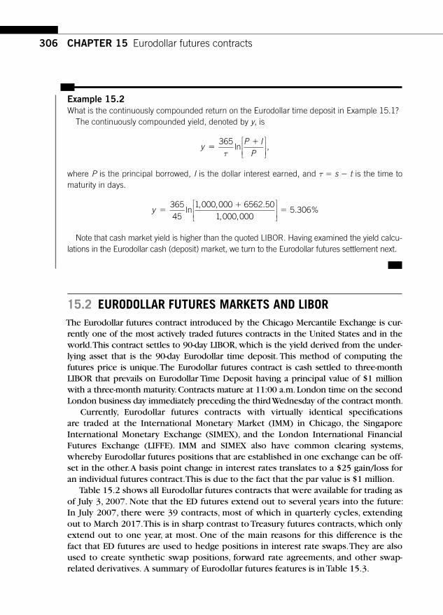
306 CHAPTER 15 Eurodollar futures contracts
Example 15.2 What is the continuously compounded return on the Eurodollar time deposit in Example 15.1?
The continuously compounded yield, denoted by y , is
yP I
P�
�365τ
ln ,⎡
⎣⎢⎢
⎤
⎦⎥⎥
where P is the principal borrowed, I is the dollar interest earned, and τ � s � t is the time to maturity in days.
y ��
�36545
1 000 000 6562 501 000 000
5 306ln, , .
, ,. %
⎡
⎣⎢⎢
⎤
⎦⎥⎥
Note that cash market yield is higher than the quoted LIBOR. Having examined the yield calcu-lations in the Eurodollar cash (deposit) market, we turn to the Eurodollar futures settlement next.
15.2 EURODOLLAR FUTURES MARKETS AND LIBOR The Eurodollar futures contract introduced by the Chicago Mercantile Exchange is cur-rently one of the most actively traded futures contracts in the United States and in the world. This contract settles to 90-day LIBOR, which is the yield derived from the under-lying asset that is the 90-day Eurodollar time deposit. This method of computing the futures price is unique. The Eurodollar futures contract is cash settled to three-month LIBOR that prevails on Eurodollar Time Deposit having a principal value of $1 million with a three-month maturity. Contracts mature at 11:00 a.m. London time on the second London business day immediately preceding the third Wednesday of the contract month.
Currently, Eurodollar futures contracts with virtually identical specifi cations are traded at the International Monetary Market (IMM) in Chicago, the Singapore International Monetary Exchange (SIMEX), and the London International Financial Futures Exchange (LIFFE). IMM and SIMEX also have common clearing systems, whereby Eurodollar futures positions that are established in one exchange can be off-set in the other. A basis point change in interest rates translates to a $25 gain/loss for an individual futures contract. This is due to the fact that the par value is $1 million.
Table 15.2 shows all Eurodollar futures contracts that were available for trading as of July 3, 2007. Note that the ED futures extend out to several years into the future: In July 2007, there were 39 contracts, most of which in quarterly cycles, extending out to March 2017. This is in sharp contrast to Treasury futures contracts, which only extend out to one year, at most. One of the main reasons for this difference is the fact that ED futures are used to hedge positions in interest rate swaps. They are also used to create synthetic swap positions, forward rate agreements, and other swap-related derivatives. A summary of Eurodollar futures features is in Table 15.3 .

307
15.2 Eurodollar futures markets and LIBOR
Table 15.2 Eurodollar Futures Prices as of July 3, 2007
Ticker Maturity(in Years)
Life Price ImpliedLIBOR
1 EDU7.Z 9/17/07 0.2 94.665 5.335
2 EDZ7.Z 12/17/07 0.5 94.700 5.300
3 EDH8.Z 3/17/08 0.7 94.775 5.225
4 EDM8.Z 6/16/08 1.0 94.825 5.175
5 EDU8.Z 9/15/08 1.2 94.830 5.170
6 EDZ8.Z 12/15/08 1.5 94.795 5.205
7 EDH9.Z 3/16/09 1.7 94.760 5.240
8 EDM9.Z 6/15/09 2.0 94.710 5.290
9 EDU9.Z 9/14/09 2.2 94.665 5.335
10 EDZ9.Z 12/14/09 2.4 94.610 5.390
11 EDH0.Z 3/15/10 2.7 94.585 5.415
12 EDM0.Z 6/14/10 2.9 94.550 5.450
13 EDU0.Z 9/13/10 3.2 94.500 5.500
14 EDZ0.Z 12/13/10 3.4 94.455 5.545
15 EDH1.Z 3/14/11 3.7 94.440 5.560
16 EDM1.Z 6/13/11 3.9 94.410 5.590
17 EDU1.Z 9/19/11 4.2 94.370 5.630
18 EDZ1.Z 12/19/11 4.5 94.330 5.670
19 EDH2.Z 3/19/12 4.7 94.310 5.690
20 EDM2.Z 6/18/12 5.0 94.280 5.720
21 EDU2.Z 9/17/12 5.2 94.245 5.755
22 EDZ2.Z 12/17/12 5.5 94.210 5.790
23 EDH3.Z 3/18/13 5.7 94.190 5.810
24 EDM3.Z 6/17/13 6.0 94.160 5.840
25 EDU3.Z 9/16/13 6.2 94.130 5.870
26 EDZ3.Z 12/15/13 6.4 94.090 5.910
27 EDH4.Z 3/15/14 6.7 94.070 5.930
28 EDM4.Z 6/14/14 6.9 94.045 5.955
29 EDU4.Z 9/15/14 7.2 94.020 5.980
(Continued)

308 CHAPTER 15 Eurodollar futures contracts
15.2.1 Eurodollar futures settlement to yields
A key feature of a Eurodollar futures contract is the way they are settled at maturity. The futures contract settles by cash on its maturity date with no delivery or timing fl exibili-ties to either the investor who is short or to the investor who is long. On the expira-tion date, which is the second London business day before the third Wednesday of the maturity month, the contract settles by cash to LIBOR using the following procedure.
On the expiration date, the clearinghouse uses the BBA LIBOR (whose fi xing was described in Section 15.1 of the chapter) to settle Eurodollar futures price at expiration.
Table 15.2 (Continued)
Ticker Maturity(in Years)
Life Price ImpliedLIBOR
30 EDZ4.Z 12/15/14 7.4 93.985 6.015
31 EDH5.Z 3/16/15 7.7 93.970 6.030
32 EDM5.Z 6/15/15 7.9 93.955 6.045
33 EDU5.Z 9/14/15 8.2 93.935 6.065
34 EDZ5.Z 12/14/15 8.4 93.905 6.095
35 EDH6.Z 3/14/16 8.7 93.885 6.115
36 EDM6.Z 6/13/16 8.9 93.865 6.135
37 EDU6.Z 9/19/16 9.2 93.845 6.155
38 EDZ6.Z 12/19/16 9.5 93.810 6.190
39 EDH7.Z 3/13/17 9.7 93.795 6.205
Source: Chicago Mercantile Exchange.
Table 15.3 Eurodollar CME Futures Contract Specifi cations
Trade unit Eurodollar time deposit having a principal value of $1 million with a three-month maturity
Point descriptions 1 point � .01 � $25
Contract listing March, June, September, December, 40 months in the March quarterly cycle, and the four nearest contract months
Product code Clearing � ED Ticker � ED
Source: Chicago Mercantile Exchange.

309
The fi nal settlement price of the Eurodollar futures contract is obtained as follows:
100 1� �( ).LIBOR (15.4)
LIBOR used in the fi nal settlement of Eurodollar futures contract is the BBA LIBOR on the settlement date and is expressed in decimals with a resolution of a basis point. For example, on September 17, 2007 (note from Table 15.2 that this is the expiry date of September 2007 futures contract), BBA fi xed 90-day LIBOR at 5.59750% (annualized). LIBOR will be expressed in decimals as 0.055975. Then the Eurodollar futures price will settle on expiry date at 100(1 � 0.055975) � 94.4025. Consequently, 100 minus the Eurodollar futures price at settlement on expiration date will be exactly the BBA LIBOR. This settlement feature of Eurodollar futures is unique and is known as the add-on settlement feature.
Note in Table 15.2 , in the last column, we have computed a quantity called implied LIBOR. This is simply 100 minus the Eurodollar futures (settlement) price on that date. Hence the implied LIBOR will converge exactly to actual BBA LIBOR at settlement on expiration date. Figure 15.1 illustrates this convergence process for the June 2007 futures contract.
The resulting Eurodollar futures price is in percentages of a face amount (1 million) of a 90-day time deposit. The market resolution is a basis point, which is worth
$ , , $ .1 000 0001
100
1
100
90
36025� � � �
15.2 Eurodollar futures markets and LIBOR
6.25
6.20
6.15
6.10
6.05
6.00
5.95
5.90
5.85
5.80
5.7511/26/1999 12/6/1999 12/16/1999 12/26/1999 1/5/2000 1/15/2000
Convergence of ED futures to BBA LIBOR
BBA Implied
FIGURE 15.1
Settlement of Eurodollar Futures to LIBOR on Maturity Date
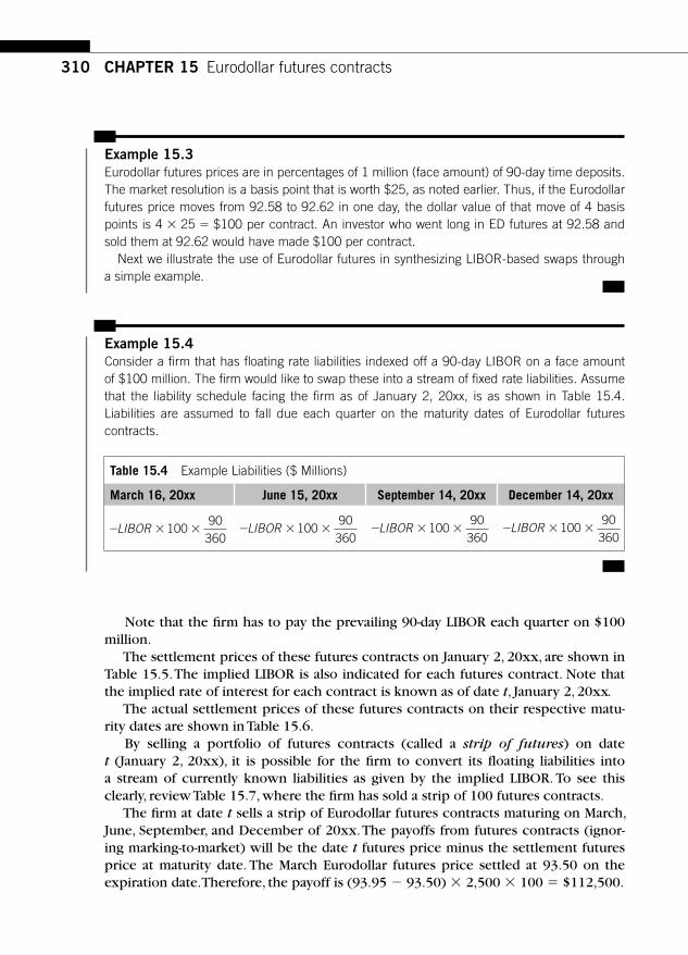
310 CHAPTER 15 Eurodollar futures contracts
Example 15.4 Consider a fi rm that has fl oating rate liabilities indexed off a 90-day LIBOR on a face amount of $100 million. The fi rm would like to swap these into a stream of fi xed rate liabilities. Assume that the liability schedule facing the fi rm as of January 2, 20 xx, is as shown in Table 15.4 . Liabilities are assumed to fall due each quarter on the maturity dates of Eurodollar futures contracts.
Table 15.4 Example Liabilities ($ Millions)
March 16, 20 xx June 15, 20 xx September 14, 20 xx December 14, 20 xx
� � �LIBOR 100
90360
� � �LIBOR 10090
360 � � �LIBOR 100
90360
� � �LIBOR 10090
360
Example 15.3 Eurodollar futures prices are in percentages of 1 million (face amount) of 90-day time deposits. The market resolution is a basis point that is worth $25, as noted earlier. Thus, if the Eurodollar futures price moves from 92.58 to 92.62 in one day, the dollar value of that move of 4 basis points is 4 � 25 � $100 per contract. An investor who went long in ED futures at 92.58 and sold them at 92.62 would have made $100 per contract.
Next we illustrate the use of Eurodollar futures in synthesizing LIBOR-based swaps through a simple example.
Note that the fi rm has to pay the prevailing 90-day LIBOR each quarter on $100 million.
The settlement prices of these futures contracts on January 2, 20xx, are shown in Table 15.5 . The implied LIBOR is also indicated for each futures contract. Note that the implied rate of interest for each contract is known as of date t, January 2, 20xx.
The actual settlement prices of these futures contracts on their respective matu-rity dates are shown in Table 15.6 .
By selling a portfolio of futures contracts (called a strip of futures) on date t (January 2, 20xx), it is possible for the fi rm to convert its fl oating liabilities into a stream of currently known liabilities as given by the implied LIBOR. To see this clearly, review Table 15.7 , where the fi rm has sold a strip of 100 futures contracts.
The fi rm at date t sells a strip of Eurodollar futures contracts maturing on March, June, September, and December of 20xx. The payoffs from futures contracts (ignor-ing marking-to-market) will be the date t futures price minus the settlement futures price at maturity date. The March Eurodollar futures price settled at 93.50 on the expiration date. Therefore, the payoff is (93.95 � 93.50) � 2,500 � 100 � $112,500.

31115.3 Deriving swap rates from ED futures
Table 15.5 ED Futures Prices as of January 2, 20xx
January 2, 20 xx March 16, 20 xx June 15, 20 xx September 14, 20 xx
December 14, 20 xx
ED futures 93.95 93.95 93.86 93.68
Implied LIBOR 6.05% 6.05% 6.14% 6.32%
Table 15.6 ED Futures Prices at Their Respective Maturity Dates
January 2, 20xx March 16, 20xx June 15, 20xx September 14, 20xx
December 14, 20xx
ED futures 93.50 93.77 92.50 91.62
Implied LIBOR 6.50% 6.23% 7.50% 8.38%
From Table 15.7 , it is clear that the LIBOR increased during this period, and as a result, the futures prices fell. We can infer this by noting that the implied LIBOR on January 2 was 6.05%, but LIBOR on the expiration date (March 16) had increased to 6.50%. The profi ts from the fall in futures prices (due to a short position in ED futures) enabled the fi rm to lock in the rates that were determined at date t. The Eurodollar futures market permitted the fi rm to lock in, at date t, the known rates as shown in the bottom row of Table 15.7 : The fi rm’s cost at each maturity date was exactly the implied LIBOR (on January 2, 20xx) of ED futures of respective matu-rity dates. For example, the actual total cost on March 16, 20xx, was exactly 6.05% applied to 100 million on a 90-day basis.
This example suggests that ED futures contracts can be used to convert fl oating liabilities denominated in LIBOR into a fi xed rate. This is the basic idea behind inter-est rate swaps.
15.3 DERIVING SWAP RATES FROM ED FUTURES The effective rate that is locked in by the fi rm, the swap rate, is computed as follows. Intuitively, the swap rate is the fi xed rate that is paid on the same dates as the fl oating payments with a present value equal to that of the fl oating payments. From Tables 15.5 and 15.7 , we see that the rates locked in as of date t were 6.05% for March, 6.05% for June, 6.14% for September, and 6.32% for December. These rates were known at date t, as shown in Table 15.5 . Intuitively, we expect that the effective (single) fi xed rate (swap rate) locked in at date t will be a weighted average of these rates implied by Eurodollar futures contracts. We proceed to compute this next.
On January 2, 20xx, LIBOR of different maturities (in the interbank market) were as shown in the fi rst row of Table 15.8 . Note that these are rates at which participat-ing banks in the interbank market were ready to borrow and lend for the term to maturity as specifi ed in row 2.

31
2C
HA
PTE
R 1
5 Eurodollar futures contracts
Table 15.7 Fixing the Cost of Floating Liabilities
Cash Flows from Futures Contracts
Transactions January 2, 20xx
March 16, 20xx June 15, 20xx September 14, 20xx December 14, 20xx
Sell 100 of each ED futures
( . . ),
6 50 6 05 25100 100 112 500
� � �
� �
( . . ),
6 23 6 05 25100 100 45 000
� � �
� �
( . . ),
7 50 6 14 25100 100 340 000
� � �
� �
( . . ),
8 38 6 32 25100 100 515 000
� � �
� �
Liabilities
� � � �
� �
6 50 10090
3601 000 000 1 625 000
. %
, , , ,
� � � �
� �
6 23 10090
3601 000 000 1 557 500
. %
, , , ,
� � � �
� �
7 50 10090
3601 000 000 1 875 000
. %
, , , ,
� � � �
� �
8 38 10090
3601 000 000 2 095 000
. %
, , , ,
Total cost
� �
� �
1 625 000 112 5001 512 500
, , ,, ,
� �
� �
1 557 500 45 0001 512 500
, , ,, ,
� �
� �
1 875 000 340 0001 535 000
, , ,, ,
� �
� �
2 095 000 515 0001 580 000
, , ,, ,

313
The discount factors prevailing as of January 2, 20xx, are in row 3 of Table 15.8 are calculated using the formula
b t jLIBOR
z( , ) .�
�
1
1360
(15.5)
In the formula contained in Equation 15.5 z is the maturity in days of LIBOR. At date t we show LIBOR quotes for settlement in March, June, September, and
December. Using this information, which is reported in Table 15.8 , we can calculate the discount factors for each of these dates. We illustrate the discount rate calcula-tions for March 16, 20xx. From Table 15.8 we note that there are 73 days between January 2, 20xx, and March 16, 20xx. LIBOR at date t for settlement at date March 16, 20xx, is 6.3125%.
Using Equation 15.5, we get the discount factor as
1
1 0 06312573
360
0 9874�
�
.. .
Table 15.8 records this information as well as the discount factors for other dates. We can compute the single fi xed rate, known as the swap rate, by discount-ing implied LIBOR that was locked up in the example and setting the sum of their present values equal to the sum of the present value of the swap rate. Let x denote the unique swap rate. Then the sum of the present value of paying x on each date is computed as follows:
0 9874 0 9723 0 9576 0 9433 3 8606. . . . . .x x x x x� � � � (15.6)
The sum of the present values of all implied LIBOR is computed as follows:
0 9874 6 05 0 9723 6 050 9576 6 14 0 9433 6 32
. ( . %) . ( . %)
. ( . %) . ( . %� � � �� � � )) . %.� 23 69749
(15.7)
15.3 Deriving swap rates from ED futures
Table 15.8 LIBOR as of January 2, 20xx
Three-MonthMaturity,
March 16, 20xx
Six-Month Maturity, June 15,
20xx
Nine-Month Maturity,
September 14, 20xx
Twelve-Month Maturity,
December 14, 20xx
LIBOR 6.3125% 6.25% 6.25% 6.25%
Days to maturity 73 164 255 346
Discount factors 0.9874 0.9723 0.9576 0.9433
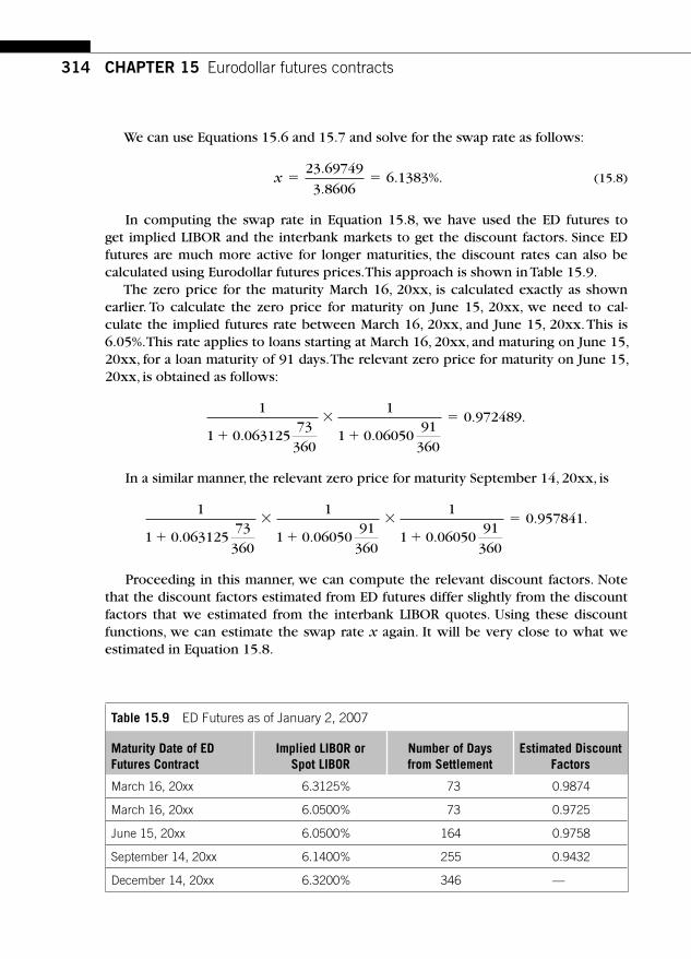
314 CHAPTER 15 Eurodollar futures contracts
We can use Equations 15.6 and 15.7 and solve for the swap rate as follows:
x � �23 69749
3 86066 1383
.
.. %. (15.8)
In computing the swap rate in Equation 15.8, we have used the ED futures to get implied LIBOR and the interbank markets to get the discount factors. Since ED futures are much more active for longer maturities, the discount rates can also be calculated using Eurodollar futures prices. This approach is shown in Table 15.9 .
The zero price for the maturity March 16, 20xx, is calculated exactly as shown earlier. To calculate the zero price for maturity on June 15, 20xx, we need to cal-culate the implied futures rate between March 16, 20xx, and June 15, 20xx. This is 6.05%. This rate applies to loans starting at March 16, 20xx, and maturing on June 15, 20xx, for a loan maturity of 91 days. The relevant zero price for maturity on June 15, 20xx, is obtained as follows:
1
1 0 06312573
360
1
1 0 0605091
360
0 972489�
�
�
�
. .. .
In a similar manner, the relevant zero price for maturity September 14, 20xx, is
1
1 0 06312573
360
1
1 0 0605091
360
1
1 0 0605091
360
0 957841�
�
�
�
�
�
. . .. .
Proceeding in this manner, we can compute the relevant discount factors. Note that the discount factors estimated from ED futures differ slightly from the discount factors that we estimated from the interbank LIBOR quotes. Using these discount functions, we can estimate the swap rate x again. It will be very close to what we estimated in Equation 15.8.
Table 15.9 ED Futures as of January 2, 2007
Maturity Date of ED Futures Contract
Implied LIBOR or Spot LIBOR
Number of Days from Settlement
Estimated Discount Factors
March 16, 20xx 6.3125% 73 0.9874
March 16, 20xx 6.0500% 73 0.9725
June 15, 20xx 6.0500% 164 0.9758
September 14, 20xx 6.1400% 255 0.9432
December 14, 20xx 6.3200% 346 —

315
15.3.1 Eurodollar futures versus swap markets
Eurodollar futures contracts can be used to execute swaps and they contain informa-tion about swap rates, but institutions fi nd it much easier to execute swaps by con-tracting swap intermediaries. There are good reasons as to why this is the case. With Eurodollar futures, the convergence to LIBOR is on the maturity date. In Chapter 16 we describe interest rate swap contracts. There we note that swaps reset to LIBOR on one date and then pay LIBOR on a different date. In addition, the reset date and payment date may not coincide with the maturity dates of ED futures contracts. For swap structures in which the rest dates and payment dates coincide with ED futures maturity dates, Eurodollar futures can be used in a direct manner.
On the other hand, the swap market is well organized, and the transactions are easily arranged. The credit risks are more easily factored into the contract. It is also easy to customize the swap contract to suit the needs of contracting parties: Arbitrary indexes, reset frequencies, and payment dates may be easily fi tted into the swap contract. However, the existence of Eurodollar futures markets and the swap rates implicit in Eurodollar futures force a tight link between swap rates and Eurodollar rates. The arbitrage possibilities between the two markets ensure a greater effi ciency in the swap market. Since most swap intermediaries hedge their risks in the Eurodollar market, the rates in these markets are linked closely. Later we show how to use ED futures contracts to value swaps by fully taking into account details of swap contracts.
15.4 INTERMARKET SPREADS Eurodollar futures are used along with other contracts such as T-bill futures contracts, T-note futures contracts, and T-bond futures contracts to implement intermarket spread strategies. The strategy using Eurodollar futures and T-bill futures contracts is referred to as TED spreads. Market participants bet on the yield gaps between bank deposits and risk-free Treasuries using TED spreads. This spread tends to widen in times of fi nancial crisis and tighten in periods of stability.
The prices of Eurodollar and T-bill futures tend to move in parallel to each other for the most part. The T-bill contract tracks the prices of deliverable T-bills. Such bills are free from default risk. The Eurodollar futures contracts track the LIBOR, and when the banking industry undergoes a downturn, LIBOR rates will increase signifi -cantly. Generally, any shock to the economy that signifi cantly affects the banking sec-tor will affect the LIBOR and, hence, the Eurodollar futures prices.
Shocks that have a systemic adverse impact on the banking sector may result in “a fl ight to quality ” in which investors liquidate their investments in banks and fl ee to “ safe ” assets, such as Treasury securities. During the Japanese bank failures of the late 1990s and the Russian default of 1998, investors exhibited their preference for Treasury securities. Under such circumstances TED spreads may dramatically widen. There is evidence that the spread between three-month LIBOR and three-month T-bills, which are the underlying instruments for ED futures and T-bill futures,
15.4 Intermarket spreads

316 CHAPTER 15 Eurodollar futures contracts
respectively, widens dramatically in periods of crisis. For example, on October 19, 1987 (the stock market crash of 1987), the spread widened to over 260 basis points. The TED spread at the beginning of January 2007 was at 25 basis points and leapt to 175 basis points by the middle of August 2007 with the onset of the credit crunch.
Other intermarket spreads with ED futures include (a) the spread between 10-year T-note futures and ED futures and (b) the spread between 30-year T-bond futures and ED futures. One of the advantages of using futures contracts to execute intermarket spreads is that they are extremely liquid.
15.5 OPTIONS ON ED FUTURES Calls and puts are traded on Eurodollar futures contracts. These contracts are listed at the IMM in the Chicago Mercantile Exchange. The settlement feature of the Eurodollar futures implies that a call option on Eurodollar futures is equivalent to a put option on LIBOR. Likewise, a put option on Eurodollar futures is equivalent to a call option on LIBOR.
To see this clearly, consider the data in Table 15.10 . On May 9, 20xx, the Eurodollar futures price is 94.48. Several calls and puts are
available on the June Eurodollar futures contract. It is important to note that these options settle by cash at maturity, and they expire on the same day as the under-lying futures contract. Let’s examine the call with a strike price of 94.25. At maturity, this call will pay an amount equal to
Max H0 94 25, . .�[ ]
We denote by H the Eurodollar futures price at maturity. We know that H � 100 � LIBOR from our discussions earlier. Using this, we get the payoff of the call option on Eurodollar futures to be
Max LIBOR0 5 75, . .�[ ]
Table 15.10 Options on June 20xx ED Futures as of May 9, 20xx
Strike Price Call Price Put Price
93.75 0.73 r
94.00 0.48 r
94.25 0.24 0.01
94.50 0.04 0.06
94.75 0.01 0.27
95.00 r 0.52

317
This is also the payoff of a put option on LIBOR with a strike rate of 5.75%. From Table 15.10 , we fi nd that this call costs 24 basis points. Each basis point costs $25 so that the value of this option is 24 � 25 � $600.
In a similar way, the put with a strike price of 94.75 will pay at maturity an amount equal to
Max H0 94 75, . .�[ ]
Again, we denote by H the Eurodollar futures price at maturity. Since at maturity, the Eurodollar futures price settles to LIBOR by the condition H � 100 � LIBOR, we can rewrite the payoff of the put at maturity as
Max LIBOR0 5 25, . .�[ ]
This is the payoff of a call option on LIBOR with a strike rate of 5.25 %. From Table 15.10 , we fi nd that this put option costs 27 basis points. Its cost is 27 � 25 � $675.
15.5.1 Caps, fl oors, and collars on LIBOR
Eurodollar futures and options on Eurodollar futures can be used to customize dif-ferent return risk profi les for investors who have assets or liabilities denominated in LIBOR. Consider Table 15.11 , in which we examine scenarios at the maturity of Eurodollar futures contracts in which LIBOR can vary from a low of 3% to a high of 8%.
Note that the Eurodollar futures price, as a consequence of its settlement to LIBOR, varies from a high of 97.00 to a low of 92.00. Table 15.11 describes the net payoffs of a long position in a call initiated at a cost of 0.24; a long position in a put initiated at a cost of 0.27; a long position in futures initiated at a futures price of 94.48; and a short position in futures initiated at a futures price of 94.48. For
15.5 Options on ED futures
Table 15.11 Payoffs of Options on ED Futures, for Various Scenarios of LIBOR at Maturity
LIBOR in % → 3.0 3.5 4.0 4.5 5.0 5.5 6.0 6.5 7.0 7.5 8.0
ED futures 97.00 96.50 96.00 95.50 95.00 94.50 94.00 93.50 93.00 92.50 92.0 0
Call K � 94.25 2.51 2.01 1.51 1.01 0.51 0.01 – 0.24 – 0.24 – 0.24 – 0.24 – 0.24
Put K � 94.75 – 0.27 – 0.27 – 0.27 – 0.27 – 0.27 – 0.02 0.48 0.98 1.48 1.98 2.48
Long ED futures 2.52 2.02 1.52 1.02 0.52 0.02 – 0.48 – 0.98 – 1.48 – 1.98 – 2.48
Short ED futures – 2.52 – 2.02 – 1.52 – 1.02 – 0.52 – 0.02 0.48 0.98 1.48 1.98 2.48
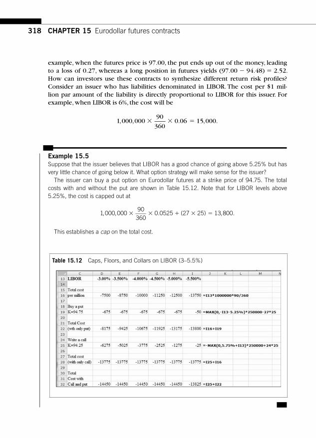
318 CHAPTER 15 Eurodollar futures contracts
Table 15.12 Caps, Floors, and Collars on LIBOR (3 –5.5%)
example, when the futures price is 97.00, the put ends up out of the money, leading to a loss of 0.27, whereas a long position in futures yields (97.00 � 94.48) � 2.52. How can investors use these contracts to synthesize different return risk profi les? Consider an issuer who has liabilities denominated in LIBOR. The cost per $1 mil-lion par amount of the liability is directly proportional to LIBOR for this issuer. For example, when LIBOR is 6%, the cost will be
1 000 00090
3600 06 15 000, , . , .� � �
Example 15.5 Suppose that the issuer believes that LIBOR has a good chance of going above 5.25% but has very little chance of going below it. What option strategy will make sense for the issuer?
The issuer can buy a put option on Eurodollar futures at a strike price of 94.75. The total costs with and without the put are shown in Table 15.12 . Note that for LIBOR levels above 5.25%, the cost is capped out at
1 000 00090
3600 0525 27 25 13 800, , . ( ) , .� � � � �
This establishes a cap on the total cost.

31915.5 Options on ED futures
If LIBOR goes below 5.25%, the issuer is able to take advantage of the falling LIBOR. The put expires, worthless. The loss is simply the put premium that was paid at the initiation date. The payoffs of the positions are shown in Figure 15.2 .
Example 15.6 What if the issuer believes that the LIBOR is likely to go up by a moderate amount but is willing to bet that it is unlikely to go down below 5.75%?
The strategy of writing a call at a strike of 94.25 will produce an income of 24 � 25 � $600 per million par. If LIBOR goes up, the issuer ends up keeping the call premium because the call fi n-ishes out of the money. This cushions the cost of the liability. If LIBOR goes down, the call ends up in the money. For example, if LIBOR � 5%, we can see from Table 15.12 that the cost is $12,500, but the call is worth [5.75 � 5.00] � 0.75, or 75 basis points. This is equal to 75 � 25 � $1275; hence, the total cost becomes 12,500 � 1,275 � 13,775. In fact, for all levels of LIBOR below 5%, the cost is $13,775. The payoffs are shown in Figure 15.3 . This establishes a fl oor on the cost.
Table 15.12 (Continued) Caps, Floors and Collars on LIBOR (6 – 8%)

320 CHAPTER 15 Eurodollar futures contracts
Cap on LIBOR at 5.25%
�14000
�13000
�12000
�11000
�10000
�9000
�8000�8.00% �7.50% �7.00% �6.50% �6.00% �5.50% �5.00% �4.50% �4.00% �3.50% �3.00%
LIBOR
Cap
ped
cost
s
FIGURE 15.2
Caps on LIBOR Using ED Futures
Floor on LIBOR at 5.75% usingcaps on ED futures
�19500
�18500
�17500
�16500
�15500
�14500
�13500�9.00% �8.00% �7.00% �6.00% �5.00% �4.00% �3.00%
LIBOR
Cos
t with
a fl
oor
at5.
75%
FIGURE 15.3
Floor on LIBOR Using ED Futures
Let’s say that the issuer would like to cap LIBOR by buying a put option on Eurodollar futures but would like to fi nance a part of this purchase by selling a call option on Eurodollar futures. In this case, the issuer would like to get a cap if LIBOR were to go up but is willing to give up some of the gains if LIBOR were to go down. This is known as a collar on LIBOR. Note from Table 15.12 that this strategy locks in a total cost of $13,200 when LIBOR goes above 5.75% and a total cost of $14,450 when LIBOR goes below 5.25%. This is illustrated in Figure 15.4 .
We can thus use Eurodollar futures and options on Eurodollar futures to create swaps, caps, fl oors, and collars on LIBOR. Since futures and options on Eurodollars are listed in exchanges, they tend to be standardized, with a limited set of maturities, strike prices, and so on. Also, they are mostly indexed to 90-day LIBOR. To get better customization, it is necessary to go to the dealer markets.
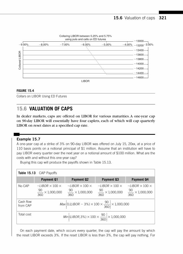
32115.6 Valuation of caps
Table 15.13 CAP Payoffs
Payment Q1 Payment Q2 Payment Q3 Payment Q4
No CAP
� � �
�
LIBOR 10090
3601 000 000, ,
� � �
�
LIBOR 10090
3601 000 000, ,
� � �
�
LIBOR 10090
3601 000 000, ,
� � �
�
LIBOR 10090
3601 000 000, ,
Cash fl ow from CAP
Max LIBOR0 3 100
90360
1 000 000,( %) , ,� � � �⎡
⎣⎢⎢
⎤
⎦⎥⎥
Total cost
Min LIBOR( , %) , ,3 100
90360
1 000 000� � �⎡
⎣⎢⎢
⎤
⎦⎥⎥
Collaring LIBOR between 5.25% and 5.75%using puts and calls on ED futures
�14600
�14400
�14200
�14000
�13800
�13600
�13400
�13200
�13000�9.00% �8.00% �7.00% �6.00% �5.00% �4.00% �3.00%
LIBOR
Col
lare
d LI
BO
R
FIGURE 15.4
Collars on LIBOR Using ED Futures
15.6 VALUATION OF CAPS In dealer markets, caps are offered on LIBOR for various maturities. A one-year cap on 90-day LIBOR will essentially have four caplets, each of which will cap quarterly LIBOR on reset dates at a specifi ed cap rate.
Example 15.7 A one-year cap at a strike of 3% on 90-day LIBOR was offered on July 15, 20xx, at a price of 110 basis points on a notional principal of $1 million. Assume that an institution will have to pay LIBOR every quarter over the next year on a notional amount of $100 million. What are the costs with and without this one-year cap?
Buying this cap will produce the payoffs shown in Table 15.13 .
On each payment date, which occurs every quarter, the cap will pay the amount by which the reset LIBOR exceeds 3%. If the reset LIBOR is less than 3%, the cap will pay nothing. For

322 CHAPTER 15 Eurodollar futures contracts
example, if at the fi rst-quarter payment date, reset LIBOR is 5%, the cap will pay (5% � 3%) � 1,000,000 � 100 � 90/360 � $500,000. The fi rm will pay 5% on $100 million, which is $1,250,000. The net cost to the fi rm will be $1,250,000 � $500,000 � $750,000, which is just 3% of the notional principal. So, the fi rm was able to cap its costs at 3%. If the reset LIBOR is below 3% in the fi rst quarter, the fi rm will have no incentive to activate the cap. The caps that apply to each payment dates are known as caplets. There are four such caplets, one for each payment date.
Black’s model of options on futures is widely used in the cap markets. In fact, in the cap market, market makers quote bid-offer spreads in terms of implied volatility. Black’s model is the basis for computing implied volatility in the cap market.
Example 15.8 Consider a cap on three-month LIBOR. Let R denote the three-month LIBOR, and let the cap rate be set at 5%. Let the notional principal be N. The cap is reset every three months. The payoff of the cap on a reset date is
N Max R14
0 5, %�[ ]
Let’s fi rst consider the general case where the cap rate is K and the interest payments are made at times shown in the following timeline:
τ 2τ
The payment at the next reset is based on LIBOR at the previous reset. That is, Rk is the rate set at kτ , and the amount paid at ( k � 1) τ is given by
N Max R K14
0, �[ ]
where N is the notional principal. Let the forward rate between kτ and ( k � 1) τ be denoted by Fk . Then the payoff of the cap can be written as of kτ as
NF
Max R Kk
ττ1
0+
[ ], �

32315.6 Valuation of caps
Table 15.14 CAP Valuation Using Black’s Formula
Recognizing that at kτ and Rk � Fk and applying Black’s model, we can price the caplet as
NF
e F N d KN dk
rkk
ττ
τ
1 1 2�
�� ( ) ( )[ ]
where
d
FK
k
k
d d k
kF
F
F
1
2
2 1
12
�
�
� �
ln;
.
⎡
⎣⎢⎢
⎤
⎦⎥⎥
τσ
σ τ
σ τ
In the next two worksheets we show how to (a) implement Black’s model on a spreadsheet, and (b) compute implied volatility. In Table 15.14 we have implemented Black’s formula for valuing a one-year cap on three-month LIBOR. Hence the cap has four caplets, each of which is priced using Black’s formula. After valuing each caplet, we simply add the four values to get the value of a one-year cap, which turns out to be $3,145.36. In valuing the cap we have taken as input the volatility of the underly-ing interest rate on which the cap is written.
Alternatively, given the market price of the cap, we can derive the implied volatil-ity as well. This is shown in Table 15.15 .
We can compute the implied volatility by equating the market price to the model price. The implied volatility is 15.18%.

324 CHAPTER 15 Eurodollar futures contracts
SUGGESTED READINGS AND REFERENCES Burghardt , G. , Belton , T. , Lane , M. , Luce , G. , & McVey , R. ( 1991) . Eurodollar futures and options:
Controlling money market risk . Probus Publishing Co.
Table 15.15 Implied Volatility of Caps

325
CHAPTER
Fixed Income Markets and Their DerivativesCopyright 2009 by Academic Press. Inc. All rights of reproduction in any form reserved.
CHAPTER SUMMARY This chapter defi nes interest rate swap contracts and introduces basic swap termi-nologies. Pricing formulas are developed for generic and forward swaps. We develop a simple arbitrage-free model for determining swap spreads and relate them to underlying economic factors. Empirical evidence is presented on swap spreads. Use of Eurodollar futures in pricing swaps and the concept of convexity adjustment are discussed. The relationship between the credit reputation of counterparties swap offer rate, swap bid rate, and the bid-offer spreads in swap markets are explained. Risk management issues pertaining to swaps are presented.
16.1 SWAPS AND SWAP-RELATED PRODUCTS AND TERMINOLOGY
Transactions in which two parties agree to make periodic payments to one another computed on the basis of specifi c interest rates on a notional principal amount are known as interest rate swaps. In most interest rate swaps, there are two legs or pay-ments: The payment made by one counterparty is based on a fl oating rate of interest, such as the LIBOR, whereas the payment made by the other counterparty is based on a fi xed rate of interest or a different fl oating interest rate. Participants in the swap market use interest rate swaps to transform one type of interest liability into another. The swap transaction is used as a tool to manage their interest rate exposure or to lock in a predetermined profi t level.
In Figure 16.1 , the basic structure of an interest rate swap is shown. Counterparty B borrows in the fl oating rate market by issuing a fi ve-year fl oater (say, at the LIBOR plus 1%), which is reset every three months. Counterparty A borrows in the fi xed
Interest-rate swaps 16

326 CHAPTER 16 Interest-rate swaps
rate market by issuing a fi ve-year note (say, at 12%). They then enter into a swap transaction with an AAA swap dealer. The swap allows B to receive a three-month LIBOR every three months. In turn, B will pay a fi xed rate of the fi ve-year Treasury plus 30 basis points. Let’s assume that the fi ve-year Treasury is yielding 11%. Then the cost to B will be 11.30%.
Counterparty A pays fl oating rate swap payments of the three-month LIBOR and receives from the swap dealer the fi ve-year Treasury plus 20 basis points. The total cost for A is 12% � 11.20% � LIBOR or LIBOR � 80 basis points.
The swap will turn out to be benefi cial if B’s borrowing cost in the fi xed rate mar-ket exceeds 12.30% and A’s borrowing cost in the fl oating rate market exceeds the LIBOR plus 80 basis points. The fl oating rate borrower (B) could be a corporation and the fi xed rate borrower (A) could be a bank. If the bank is in a better position to monitor and manage A’s risks, a bilateral contract, such as a swap, could benefi t both parties. For example, B may have an informational advantage relative to the typical fl oating rate lender. Moreover, B is in the business of evaluating the risks of borrow-ers and, as a result, may have acquired greater monitoring and risk-management skills over time. In addition, B, being a bank, might also have a supply of borrowers with differing borrowing requirements. As a result, B’s search costs are lower in terms of identifying and matching two counterparties with complementary borrowing needs. For this service, B typically gets a fee. The advantages of better information and lower transactions costs (of monitoring, for instance) are refl ected in the swap transaction. The foregoing observations suggest that it is necessary to admit differential informa-tion and the costs of monitoring and searching to rationalize a swap transaction.
16.1.1 Asset swaps
Swaps can also be arranged to manage the risk of specifi c asset or liability exposures. An asset swap , for example, combines an existing asset, such as a bond or a note,
A B
Swap dealer has a matched book. The dealer receives on the swapoffer side T�30 bps, and pays on the swap bid side T�20 bps.
Swap dealer(AAA rated)
Term: 5 yearsIndex: 3-months LIBOR
LIBOR
T�30 bps
LIBOR
T�20 bps
T � Five-year benchmark Treasury yield
FIGURE 16.1
Swap Transaction: Basic Terminology

327
with a swap to create a different risk-return profi le. Consider an investor who owns a fi xed rate asset. He can engage in an interest rate swap as shown in Figure 16.2 .
The investor swaps the coupons with the swap dealer for fl oating rate revenues. If the fi xed rate asset held by the investor is highly illiquid, the swap may allow the investor to “ trade ” the cash fl ows of this illiquid asset at a competitive fl oating rate.
The underlying asset used in an asset swap can be a zero coupon bond, a CMO, or a premium or a discount bond. This implies that the swap payments and netting of cash fl ows between the counterparties can vary to suit the counterparties ’ needs. If the asset is a mortgage-backed security, it will be paying monthly cash fl ows that go toward interest and amortizing principal payments. Such assets can be combined with index amortizing swaps , where the notional principal is amortized to pre-cisely mirror the asset’s remaining principal amount.
16.1.2 Diversity of swap contracts
In addition to the size of the swap markets, the diversity of contracts that are struc-tured in the market bears some attention. Swaps are structured on various underly-ing instruments with varying maturity dates. To gain a perspective on the diversity of this market, examine Table 16.1 .
There are fi ve basic types of swaps: fi xed-to-fl oating in the same currency, fl oat-ing-to-fl oating in the same currency, their counterparts across two currencies, and currency swaps that are fi xed-to-fi xed. In addition, there are markets that are closely related to swap markets:
■ Interest-rate caps. This agreement caps the interest obligations at a predeter-mined rate for a prespecifi ed period of time. For example, Firm A agrees to sell a cap on a three-month LIBOR at 6.5% for every quarter for the next two years. In return, Firm B pays Firm A an agreed-on compensation.
16.1 Swaps and swap-related products and terminology
Coupon
Fixed rate
LIBOR
Asset swaps allow investors totransform the cash flowsof existing assets.
Fixed ratebond
Investor Dealer
FIGURE 16.2
Asset Swaps

328 CHAPTER 16 Interest-rate swaps
■ Swaptions. Bank A may sell an option to Bank B, whereby Bank B will have the option to enter into a swap any time before a predetermined date at predeter-mined terms of exchange.
■ Floor. An investor holding a portfolio of fl oating rate notes for which the cou-pons are indexed to LIBOR might want to buy a fl oor on LIBOR. If the fl oor rate is 6% and LIBOR falls below 6%, the difference is paid to the investor on the agreed-on notional principal.
The swap-related products, such as caps, fl oor, and swaptions, are dealer market products. Since they are highly customized, they differ from the caps and fl oors discussed earlier in the context of options on Eurodollar futures contracts. These Eurodollar futures options are standardized (90-day LIBOR, fi xed strike prices, and maturities) and are not liquid beyond six months.
16.2 VALUATION OF SWAPS In this section, a framework is developed for the valuation of swaps. To value swaps, we fi rst establish some conventions. The reset period (frequency) of the swap refers to the frequency with which the fl oating leg of the swap is reset. If the fl oating leg of the swap is reset every three months, it is said to have a reset frequency of three months. The index maturity of the swap refers to the underlying LIBOR maturity: If the fl oating leg is indexed to three-month LIBOR, the swap is said to have an index maturity of three months. The payment lag is the time lag between the reset date and payment date. If the fl oating leg of the swap is reset to three-month LIBOR now and the actual payment is made after three months, it is said to have a payment lag
Table 16.1 Diverse Swap Contracts
Type of Swap Term of Swap Attributes
Plain-vanilla interest rate swaps 1–30 years Same currency; one party pays fi xed and the other fl oating
Basis swaps 1–10 years Same currency; parties pay fl oating cash fl ows linked to different indexes
Currency swaps —fi xed to fi xed 2–10 years Different currencies; both parties pay fi xed rates
Currency swaps —fi xed to fl oating 2–10 years Different currencies; one party pays fi xed and the other fl oating
Currency swaps —fl oating to fl oating 2–10 years Different currencies; both parties pay fl oating rates

329
of three months. These conventions are shown for a generic interest rate swap in Figure 16.3 .
Most interest rate swaps are known as generic interest rate swaps. In such swaps, typically the fl oating index is three-month LIBOR. Also in these swaps, the reset date precedes the payment date by exactly the index maturity (three months). For generic interest rate swaps, the settlement date is typically the fi rst reset date. We illustrate the general principles of valuing generic interest rate swaps with a simple example next.
Example 16.1 In Table 16.2 , swap reset dates and payment dates are indicated, along with zero coupon prices estimated from the market. The fi rst reset date is October 27, 1995, which is also the settlement date. The fi rst payment date is January 27, 1996, and so on, as indicated in Table 16.2 . What is the one-year swap rate in which fl oating and fi xed payments are made every quarter?
16.2 Valuation of swaps
First reset date
Second reset date andthe first payment date
Third reset date andthe second payment date
FIGURE 16.3
Generic Interest Rate Swap
Table 16.2 Conventions in Generic Interest Rate Swaps
Settlement Date, October 27, 1995 First Reset Date Is Settlement Date
Zero Price Maturity Date
1 0.975 January 27, 1996 First payment date and second reset date
2 0.945 April 27, 1996 Second payment date and third reset date
3 0.923 July 27, 1996 Third payment date and fourth reset date
4 0.914 October 27, 1996 Fourth and fi nal payment date
Using the zero prices, we can determine the 90-day forward rates as of each reset date in the following manner. Let f (1, 2) be the forward rate between fi rst reset date and the second reset date. Since the fi rst reset date is also the current settlement

330 CHAPTER 16 Interest-rate swaps
date, f(1,2) is simply the spot rate between date 0 and date 1, which is related to the zero price as follows. (We assume that the time between two resets is one quarter or 1/4 of a year.)
0 9751
11 2
4
1 2 41
0 9751 10 256.
( , )( , )
..�
�
� � �f
f⎛⎝⎜⎜⎜
⎞⎠⎟⎟⎟
⇒⎡
⎣⎢⎢
⎤
⎦⎥⎥
44%
The forward rate between the second reset date and the third reset date is denoted by f (2,3) and is determined as follows.
0 9451
11 2
41
2 3
4
1
10 102564
4
.( , ) ( , ) .
�
� �
�
�f f⎛
⎝⎜⎜⎜
⎞⎠⎟⎟⎟⎛⎝⎜⎜⎜
⎞⎠⎟⎟⎟
⎛⎛⎝⎜⎜⎜
⎞⎠⎟⎟⎟⎛⎝⎜⎜⎜
⎞⎠⎟⎟⎟1
2 3
4�
f ( , ).
This can be solved for the required forward rate as follows:
0 9450 975
12 3
4
2 3 40 975
0 9451.
.
( , )( , )
.
.�
�
� �f
f⎛⎝⎜⎜⎜
⎞⎠⎟⎟⎟
⇒⎡
⎣⎢⎢
⎤
⎦⎥⎥⎥
� 12 6984. %.
In a similar way, the forward rate between the third reset date and the fourth reset date denoted by f (3,4) may be determined as follows:
0 9231
11 2
41
2 3
41
3 4
4
.( , ) ( , ) ( , )
�
� � �f f f⎛
⎝⎜⎜⎜
⎞⎠⎟⎟⎟⎛⎝⎜⎜⎜
⎞⎠⎟⎟⎟⎛⎝⎜⎜⎜⎜
⎞⎠⎟⎟⎟
⎛⎝⎜⎜⎜
⎞⎠⎟⎟⎟⎛⎝⎜⎜⎜
⎞⎠⎟⎟⎟
�
� � �
1
10 102564
41
0 126984
41
3 4. . ( ,f )).
4
⎛⎝⎜⎜⎜
⎞⎠⎟⎟⎟
This can be solved for the required forward rate as follows:
0 9230 945
13 4
4
3 4 40 945
0 9231.
.
( , )( , )
.
.�
�
� �f
f⎛⎝⎜⎜⎜
⎞⎠⎟⎟⎟
⇒⎡
⎣⎢⎢
⎤
⎦⎥⎥⎥
� 9 5341. %.
Finally, proceeding in the same manner, we can determine the forward rate between the fourth and fi nal reset date and the fi nal payment date as follows:
0 9140 923
14 5
4
4 5 40 923
0 9141.
.
( , )( , )
.
.�
�
� �f
f⎛⎝⎜⎜⎜
⎞⎠⎟⎟⎟
⇒⎡
⎣⎢⎢
⎤
⎦⎥⎥⎥
� 3 9387. %.
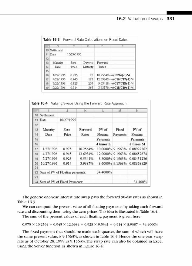
331
The generic one-year interest rate swap pays the forward 90-day rates as shown in Table 16.3 .
We can compute the present value of all fl oating payments by taking each forward rate and discounting them using the zero prices. This idea is illustrated in Table 16.4 .
The sum of the present values of each fl oating payment is given here:
0.975 � 10.2564 � 0.945 � 12.6984 � 0.923 � 9.5341 � 0.914 � 3.9387 � 34.4000%
The fi xed payment that should be made each quarter, the sum of which will have the same present value, is 9.1563%, as shown in Table 16.4 . Hence the one-year swap rate as of October 28, 1999, is 9.1563%. The swap rate can also be obtained in Excel using the Solver function, as shown in Figure 16.4 .
16.2 Valuation of swaps
Table 16.3 Forward Rate Calculations on Reset Dates
Table 16.4 Valuing Swaps Using the Forward Rate Approach

332 CHAPTER 16 Interest-rate swaps
One last point should be made concerning this example, which turns out to be much more general. Consider a one-year bond that pays 5.1563% every quarter and $1 at the end of one year. At what price should this bond sell on October 28, 2007?
The sum of the present values of all quarterly fi xed coupons plus the present value of the fi nal balloon payment of $1 is shown here:
9 1563
40 975 0 945 0 923 0 914 1 0 914 1
. %. . . . . .� � � � � � �[ ]
This result, which is rather general, says that the coupon of a one-year bond that sells at par is in fact the generic swap rate. Since the coupon of a bond that sells at par is its yield to maturity, we can say that the generic swap rate of a swap with T years term is the T-year par bond yield.
We use this insight in Table 16.5 to provide a general way to value swaps. In Table 16.5 , we go long in a par bond that pays a coupon of S every six months.
Our investment at date 0 is exactly the par value, which is 1. We fi nance the purchase of this par bond by shorting a default-free fl oating rate note that resets at date 0. Since the fl oating rate note resets at date 0, it will sell at par as well. The fl oater is reset at
FIGURE 16.4
Finding Swap Rate Using Excel Solver

333
date 0 to the three-month LIBOR that prevailed at date 0. We denote this as LIBOR (0). This is paid to the owner of the fl oating rate note three months from date 0, which is date 0.25. The fl oating rate note then resets at date 0.25 to the then-prevailing LIBOR, which we denote by LIBOR (0.25). This is paid at date 0.50, and so on.
Note that the short seller of the fl oating rate note will pay the owner all the fl oat-ing coupon payments as shown in Table 16.5 . His total cash fl ows are presented in the last row of Table 16.5 . The total cash fl ows from the portfolio are exactly equal to what we would get in a one-year swap in which we receive three-month LIBOR every quarter (with a lag of three months) and pay fi xed every six months. The pre-vious arguments imply that the one-year swap rate, S, is the coupon on the one-year par bond, which is the one-year par bond yield!
We can use the discount factors to compute the present value of the coupons of the par bond and set the sum of the present values of all cash fl ows equal to par (or one). We will use the following convention in describing the zeroes. Let b ( t , s) denote the dollar price of a zero coupon bond at date t . The bond pays $1 at maturity date s.
The valuation formula for a one-year par bond is:
Sb S b( , . ) [ ] ( , ) .0 0 5 1 0 1 1� � � (16.1)
Solving Equation 16.1 for S , we get the formula for the swap rate:
Sb
b b�
�
�
1 0 1
0 0 5 0 1
( , )
( , . ) ( , ). (16.2)
This formula generalizes easily to an N -year swap as follows:
Sb N
b b b N�
�
� �
1 0
0 0 5 0 1 0
( , )
( , . ) ( , ) ( , ).
…(16.3)
16.2 Valuation of swaps
Table 16.5 General Approach to Pricing Generic Interest Rate Swaps
Swap � A Long in a Fixed Rate Par Bond Plus a Short in a Floating Rate Note
< -------- Reset and Payment Dates -------- >
0 0.25 0.5 0.75 1
Buy a one-year par bond paying a coupon of S every six months
� 1 S S � 1
Short a one-year FRN resetting and paying LIBOR every quarter with a lag of one quarter
1 �LIBOR(0) �LIBOR(0.25) �LIBOR(0.50) 1 � LIBOR(0.75)
Total cash fl ows 0 �LIBOR(0) S � LIBOR(0.25) �LIBOR(0.50) S � LIBOR(0.75)
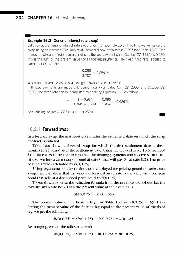
334 CHAPTER 16 Interest-rate swaps
Example 16.2 (Generic interest rate swap) Let’s revisit the generic interest rate swap pricing of Example 16.1. This time we will price the swap using only zeroes. The sum of all (zeroes) discount factors is 3.757 (see Table 16.3 ). One minus the discount factor corresponding to the last payment date (October 27, 1996) is 0.086; this is the sum of the present values of all fl oating payments. The swap fi xed rate (applied to each quarter) is then:
0 0863 757
2 2891..
. %.�
When annualized, (2.2891 � 4), we get a swap rate of 9.1562%. If fi xed payments are made only semiannually (on dates April 28, 2000, and October 28,
2000), the swap rate can be computed by applying Equation 16.2 as follows:
S ��
�� �
1 0 9140 945 0 914
0 0861 859
4 626.
. ...
. %.
Annualizing, we get 4.6525% � 2 � 9.252%.
16.2.1 Forward swap
In a forward swap, the fi rst reset date is after the settlement date on which the swap contract is initiated.
Table 16.6 shows a forward swap for which the fi rst settlement date is three months (0.25 years) after the settlement date. Using the ideas of Table 16.5 , we need $1 at date 0.25 to be able to replicate the fl oating payments and receive $1 at matu-rity. So, we buy a zero coupon bond at date 0 that will pay $1 at date 0.25. The price of such a zero is denoted by b (0,0.25).
Using arguments similar to the those employed for pricing generic interest rate swaps, we can show that the one-year forward swap rate is the yield on a one-year bond that sells at a discounted price equal to b (0,0.25) .
To see this, let’s write the valuation formula from the previous worksheet. Let the forward swap rate be S . Then the present value of the fi xed leg is
Sb Sb( , . ) ( , . ).0 0 75 0 1 25�
The present value of the fl oating leg from Table 16.6 is b(0,0.25) � b (0,1.25). Setting the present value of the fl oating leg equal to the present value of the fi xed leg, we get the following:
Sb Sb b b( , . ) ( , . ) ( , . ) ( , . ).0 0 75 0 1 25 0 0 25 0 1 25� � �
Rearranging, we get the following result:
Sb Sb b b( , . ) ( , . ) ( , . ) ( , . ).0 0 75 0 1 25 0 1 25 0 0 25� � �

335
Or, the swap rate is the yield on a bond selling at a price of b (0,0.25)! Solving, we get the swap rate as follows:
Sb b
b b�
�
�
( , . ) ( , . )
( , . ) ( , . ).
0 0 25 0 1 25
0 0 75 0 1 25(16.4)
More generally, for a forward swap starting y periods from the settlement date and maturing in N years, we get the valuation formula shown here:
Sb y b N
b ii y
N�
�
� �
( , ) ( , )
( , )
.
.
0 0
00 5
∑
Example 16.3 (Forward swaps) Consider the previous example. If the fi rst reset date of the swap is January 28, 2000, and the swap had a one-year maturity, what is the swap rate? Why?
The sum of all four discount factors from April 28, 2000, maturity to January 28, 2001, maturity is 3.677. The price of a discount factor maturing on January 28, 2000, minus the price of a discount factor maturing on January 28, 2001, is 0.0800. The forward swap rate applicable to every quarter is (by formula) 2.1757%. On an annualized basis, the swap rate is 2.1757% � 4, or 8.703%.
16.2 Valuation of swaps
Table 16.6 General Approach to Pricing Forward Swaps
� -------Reset and Payment Dates -------- �
0 0.25 First reset
0.5 0.75 1 1.25
Buy a zero coupon
bond maturing on
date 0.25; use the
proceeds ($1) at
date 0.25 to invest in
three-month LIBOR
� b (0,0.25) LIBOR(0.25) LIBOR(0.50) LIBOR(0.75) LIBOR(1) � 1
Short a zero coupon
bond maturing on
date 1.25
� b (0,1.25) � 1
Total cash fl ows � b (0,1.25) � b(0,0.25) LIBOR(0.25) LIBOR(0.50) LIBOR(0.75) LIBOR(1)
PV of fl oating leg b (0, 0.25) � b (0,1.25)

336 CHAPTER 16 Interest-rate swaps
16.2.2 ED futures and swap pricing
We can utilize the ED futures contracts to value forward swaps. This is shown with the following example.
Example 16.4 The settlement date is February 25, and the Eurodollar futures prices are shown in Table 16.7 . Based on this information, how will you determine the one-year swap rate on a forward swap that starts on March 19, 2000, and ends on March 19, 2001? The swap’s reset date precedes the payment date by one quarter. Assume that the start date (February 25, 2000) is the fi rst reset date. Assume that the spot LIBOR between February 25, 2000, and March 19, 2000, is 6.040%.
Table 16.7 Schedule of Example Eurodollar Futures Prices
SD Maturity February 25, 2000, Settlement Price
03/19/00 93.798
06/19/00 93.480
09/19/00 93.255
12/19/00 93.025
03/19/01 92.920
06/18/01 92.820
09/17/01 92.765
12/17/01 92.700
03/18/02 92.735
06/17/02 92.725
09/16/02 92.720
12/16/02 92.655
Source: Chicago Mercantile Exchange.
To value swaps using ED futures, we need to make two adjustments. First, it should be recognized that swaps reset a quarter earlier to the actual payment date. In ED futures, cash settlement to LIBOR occurs without any delay on the maturity date. This means that the ED futures price for March 19, 2000, should be used to arrive at the payment in the swap as of June 19, 2000. Next, swaps are like par bonds and therefore they have convexity (see Chapter 7). ED futures settle to LIBOR linearly in the sense that one basis point movement is worth $25 under all circumstances.

337
So, we need to make a convexity adjustment to value swaps using ED futures. We proceed to discuss these corrections.
Eurodollar futures prices shown in Table 16.7 are rounded to three decimals. In calculations, we have used the actual prices.
Since the payment date follows the reset date by one quarter, we need to use the Eurodollar futures price for specifi c maturity to determine LIBOR three months later. For example, we use the futures contract corresponding to the maturity date of March 19, 2000 (the start date), to determine the forward rate on June 19, 2000 (the fi rst payment date). In Table 16.7 , the forward rate at June 19, 2000, is 100 � 93.798 � 6.203 (rounded up). The actual spot LIBOR is used for computing the forward price between the settlement date and March 19, 2000.
We illustrate some of the calculations in the spreadsheet in Table 16.8 . Cell G14 contains the zero price as of February 25, 2000, for maturity on March 19, 2000. This is computed as follows:
100
1 0 060423
360
99 616� �
�
.. .
16.2 Valuation of swaps
Table 16.8 Using Eurodollar Futures to Compute Discount Factors
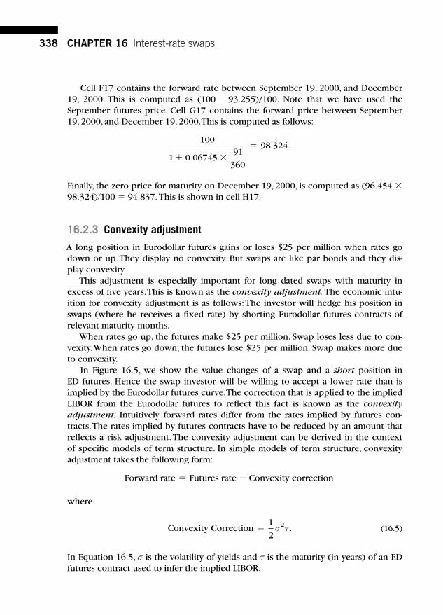
338 CHAPTER 16 Interest-rate swaps
Cell F17 contains the forward rate between September 19, 2000, and December 19, 2000. This is computed as (100 � 93.255)/100. Note that we have used the September futures price. Cell G17 contains the forward price between September 19, 2000, and December 19, 2000. This is computed as follows:
100
1 0 0674591
360
98 324� �
�
.. .
Finally, the zero price for maturity on December 19, 2000, is computed as (96.454 � 98.324)� 100 � 94.837. This is shown in cell H17.
16.2.3 Convexity adjustment
A long position in Eurodollar futures gains or loses $25 per million when rates go down or up. They display no convexity. But swaps are like par bonds and they dis-play convexity.
This adjustment is especially important for long dated swaps with maturity in excess of fi ve years. This is known as the convexity adjustment. The economic intu-ition for convexity adjustment is as follows: The investor will hedge his position in swaps (where he receives a fi xed rate) by shorting Eurodollar futures contracts of relevant maturity months.
When rates go up, the futures make $25 per million. Swap loses less due to con-vexity. When rates go down, the futures lose $25 per million. Swap makes more due to convexity.
In Figure 16.5 , we show the value changes of a swap and a short position in ED futures. Hence the swap investor will be willing to accept a lower rate than is implied by the Eurodollar futures curve. The correction that is applied to the implied LIBOR from the Eurodollar futures to refl ect this fact is known as the convexity adjustment. Intuitively, forward rates differ from the rates implied by futures con-tracts. The rates implied by futures contracts have to be reduced by an amount that refl ects a risk adjustment. The convexity adjustment can be derived in the context of specifi c models of term structure. In simple models of term structure, convexity adjustment takes the following form:
Forward rate Futures rate Convexity correction� �
where
Convexity Correction1
2� σ τ2 . (16.5)
In Equation 16.5, σ is the volatility of yields and τ is the maturity (in years) of an ED futures contract used to infer the implied LIBOR.

339
16.3 SWAP SPREADS The difference between the fi xed rate on a swap and the yield of the underlying Treasury benchmark with the same maturity is known as the swap spread. Swap spreads are presented in Table 16.9 .
For the 10-year maturity, the Treasury benchmark yielded 4.06%. The swap spread on the bid side was 75.5 basis points. Therefore, the bid swap rate was
16.3 Swap spreads
Swap and EDfutures value
ED futuresvalue
Rates
Swap value
�1bp��25
�1bp��25
FIGURE 16.5
Convexity Adjustment
Table 16.9 Swap Spreads as of July 18, 2008
Treasury Swaps
Benchmark Price Yield Swap Rate Swap Spreads Bid/Offer
2-year 100:165 2.50% 3.58% 97.2/98.2
5-year 100:015 3.36% 4.35% 97.8/98.8
10-year 98:172 4.06% 4.81% 74.5/75.5
30-year 95.232 4.64% 5.11% 46.0/47.0
Source: Lehman Brothers.

340 CHAPTER 16 Interest-rate swaps
4.06% � 0.755 � 4.815%. The swap spread on the offer side was 74.5 basis points; hence, the swap offer rate was 4.06% � 0.745 � 4.805%. Note that the swap rates are quoted against three-month LIBOR. Swap spreads are inverted in the sense that the 10- and 30-year swap spreads are lower than the short-term swap spreads.
To get a perspective on swap spreads, we look at the historical data in Figure 16.6 from 1990 to 2000 and in Figure 16.7 for a more recent period, from 2003 to 2008.
Table 16.10 summarizes swap spreads for two sub-samples. During the sample period 1990 –2000, the average swap spreads ranged from 33 to 42 basis points.
Swap spreads in basis points
525456585
Sw
ap s
prea
ds 105125145
10/19/89 7/15/92 4/11/95 1/5/98 10/1/001990–2000
2-year 5-year 10-year
FIGURE 16.6
History of Swap Spreads, 1990 –2000
Swap spreads in basis points
102030405060708090
100110
5/21/03 10/2/04 2/14/06 6/29/07 11/10/082003–2008
Sw
ap s
prea
ds
2-year 5-year 10-year
FIGURE 16.7
History of Swap Spreads, 2003 –2008

341
In the sample period 2003 –2008, the average swap spreads ranged between 47 to 52 basis points.
During the banking (savings and loan) crisis in the late 1980s, swap spreads were elevated. They started to contract to a low around 1992 and remained at fairly low levels during 1992 through 1996. The onset of the crisis in Asia in 1997, followed by Russian default and the LTCM collapse in 1998, contributed to widening swap spreads. The budget surplus and the resulting contraction of the Treasury debt in 2000 further elevated swap spreads. To understand these patterns, we need to exam-ine the determinants of swap spreads, to which we turn now.
The following factors infl uence swap spreads: The prevailing and the expected spread between the fi nancing rate and the
London interbank offered rates or the LIBOR –REPO spread is an important factor affecting the swap spreads.
Dealers hedge open positions in swaps using either the Eurodollar futures con-tracts or Treasury securities. For swaps with a maturity of fi ve years or more, it is reasonable to think that Treasury securities are used as hedging instruments, given unavailability or the poor liquidity of Eurodollar futures for such a maturity range.
A dealer who receives fi xed in the swap will hedge by shorting the underlying Treasury. This way the swap spread is locked in and the dealer’s incremental cost is the difference between LIBOR (which he or she pays) and the reverse repo rate (that he or she earns on the cash collateral). As this spread widens, the cost associ-ated with the hedge increases, and the dealer will want a higher swap spread to compensate for this cost. This is illustrated in Figure 16.8 .
The swap dealer hedges his or her swap by shorting the benchmark Treasury. Let’s say that the Treasury benchmark is yielding 6.0%, resulting in a swap spread of 50 basis points. The dealer’s income and expenses are summarized in Table 16.11 .
Note from Table 16.11 that the total income to the dealer decreases as LIBOR to repo spread increases. Hence with widening LIBOR to repo spread, the dealer would want to charge a higher swap spread.
16.3 Swap spreads
Table 16.10 Summary of History of Swap Spreads
Summary Statistics on Swap Spreads (1990 – 2000) in Basis Points
Summary Statistics on Swap Spreads (2003 – 2008) in Basis Points
Two-Year Five-Year Ten-Year Two-Year Five-Year Ten-Year
Maximum 88 88 101 110 111 90
Minimum 9 9 14 19 35 36
Average 33 33 42 47 52 52
Median 29 29 34 41 47 51
Volatility 16 16 20 17 15 10
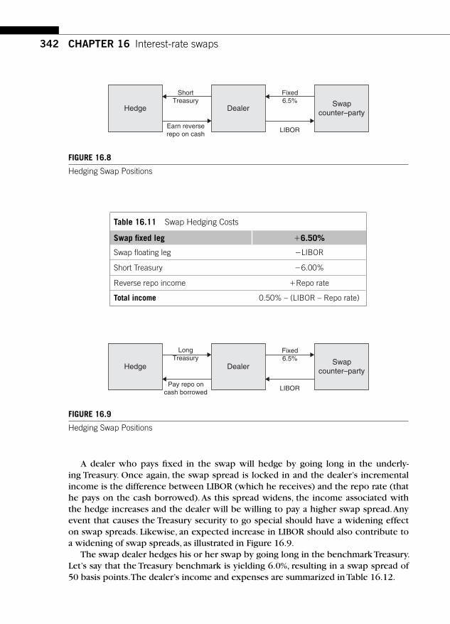
342 CHAPTER 16 Interest-rate swaps
A dealer who pays fi xed in the swap will hedge by going long in the underly-ing Treasury. Once again, the swap spread is locked in and the dealer’s incremental income is the difference between LIBOR (which he receives) and the repo rate (that he pays on the cash borrowed). As this spread widens, the income associated with the hedge increases and the dealer will be willing to pay a higher swap spread. Any event that causes the Treasury security to go special should have a widening effect on swap spreads. Likewise, an expected increase in LIBOR should also contribute to a widening of swap spreads, as illustrated in Figure 16.9 .
The swap dealer hedges his or her swap by going long in the benchmark Treasury. Let’s say that the Treasury benchmark is yielding 6.0%, resulting in a swap spread of 50 basis points. The dealer’s income and expenses are summarized in Table 16.12 .
Hedge Dealer
LongTreasury
Pay repo oncash borrowed
Fixed6.5%
LIBOR
Swapcounter–party
FIGURE 16.9
Hedging Swap Positions
Hedge Dealer
ShortTreasury
Earn reverserepo on cash
Fixed6.5%
LIBOR
Swapcounter–party
FIGURE 16.8
Hedging Swap Positions
Table 16.11 Swap Hedging Costs
Swap fi xed leg � 6.50%
Swap fl oating leg � LIBOR
Short Treasury � 6.00%
Reverse repo income � Repo rate
Total income 0.50% – (LIBOR – Repo rate)
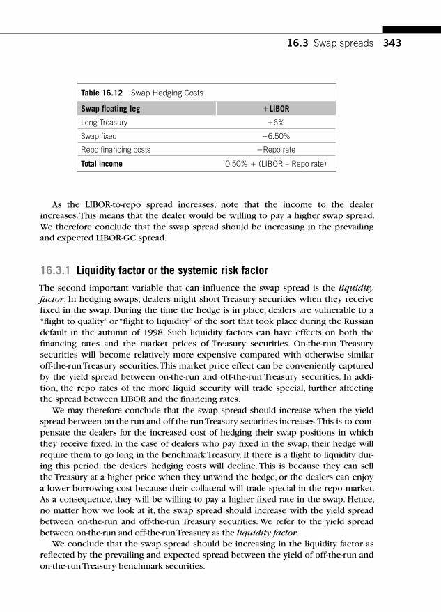
343
As the LIBOR-to-repo spread increases, note that the income to the dealer increases. This means that the dealer would be willing to pay a higher swap spread. We therefore conclude that the swap spread should be increasing in the prevailing and expected LIBOR-GC spread.
16.3.1 Liquidity factor or the systemic risk factor
The second important variable that can infl uence the swap spread is the liquidityfactor. In hedging swaps, dealers might short Treasury securities when they receive fi xed in the swap. During the time the hedge is in place, dealers are vulnerable to a “ fl ight to quality ” or “ fl ight to liquidity ” of the sort that took place during the Russian default in the autumn of 1998. Such liquidity factors can have effects on both the fi nancing rates and the market prices of Treasury securities. On-the-run Treasury securities will become relatively more expensive compared with otherwise similar off-the-run Treasury securities. This market price effect can be conveniently captured by the yield spread between on-the-run and off-the-run Treasury securities. In addi-tion, the repo rates of the more liquid security will trade special, further affecting the spread between LIBOR and the fi nancing rates.
We may therefore conclude that the swap spread should increase when the yield spread between on-the-run and off-the-run Treasury securities increases. This is to com-pensate the dealers for the increased cost of hedging their swap positions in which they receive fi xed. In the case of dealers who pay fi xed in the swap, their hedge will require them to go long in the benchmark Treasury. If there is a fl ight to liquidity dur-ing this period, the dealers ’ hedging costs will decline. This is because they can sell the Treasury at a higher price when they unwind the hedge, or the dealers can enjoy a lower borrowing cost because their collateral will trade special in the repo market. As a consequence, they will be willing to pay a higher fi xed rate in the swap. Hence, no matter how we look at it, the swap spread should increase with the yield spread between on-the-run and off-the-run Treasury securities. We refer to the yield spread between on-the-run and off-the-run Treasury as the liquidity factor.
We conclude that the swap spread should be increasing in the liquidity factor as refl ected by the prevailing and expected spread between the yield of off-the-run and on-the-run Treasury benchmark securities.
16.3 Swap spreads
Table 16.12 Swap Hedging Costs
Swap fl oating leg � LIBOR
Long Treasury �6%
Swap fi xed � 6.50%
Repo fi nancing costs � Repo rate
Total income 0.50% � (LIBOR – Repo rate)

344 CHAPTER 16 Interest-rate swaps
16.3.2 Credit risk in the bank sector
Banks infl uence swap spreads in two important ways. Banks actively use the swap market for their asset-liability management purposes. Banks use swaps to con-vert their fl oating rate assets into fi xed. This makes them a receiver of fi xed in the swap market. The level of their participation, therefore, infl uences swap spreads. In addition, the London interbank offered rate is determined by the British Bankers Association (BBA). (The details of LIBOR fi xing are readily found at www.bba.org.uk.) Since LIBOR is typically the index used in the fl oating leg of swaps, the overall or systemic risk of the banks infl uence swap spreads as well. The panel contributes rates to BBA, and the rates are ranked. Only the rates in the middle quartiles are used in a simple arithmetic averaging process to fi x LIBOR. Therefore, LIBOR refl ects the average credit quality of this contributing panel of banks and the way BBA makes adjustments to this panel as the credit reputation of these banks changes. From the perspective of understanding the swap spreads, the following aspects of LIBOR are critical: First, LIBOR refl ects the average credit risk of the panel banks. As the aver-age credit quality falls, we can expect LIBOR to go up as investors demand a higher compensation for assuming increased credit risk. Second, though LIBOR refl ects the average credit quality of the panel of banks, the swap contract is typically “credit enhanced. ” Daily losses in swaps are met by posting collateral on a daily basis. On each payment date, the losses and gains are netted, and the position is marked to market. To a fi rst approximation, then, it seems reasonable to assume that the swap has little or no credit risk. It then follows that the swap rate must increase when the average credit quality of the panel banks decreases! This conclusion has important implications for valuing swaps and understanding swap spreads. This line of reason-ing suggests that the modeling of credit risk is important in the valuation of swaps, not because we believe that the swap has credit risk but only because the panel of banks in LIBOR fi xing has default risk.
We should recognize an important caveat to the arguments presented here: If the bank sector as a whole were to experience a serious systemic risk exposure of the sort that occurred following the hedge funds failures in the autumn of 1998, inves-tors would become more risk averse. As a result, swap spreads will inherit a default risk premium.
16.3.3 Agency activities
The volume of agency issues and their mortgage-backed securities portfolio should be a big factor in swap spreads, but no unambiguous sign could be attached to swap spreads as a result of the activities of the agencies in the swap market. This is because the agencies could potentially be on either side of swap transactions. To the extent that agencies attempt to remain neutral by matching the duration of their assets (which are mortgages and MBS) with their liabilities (which are debt securi-ties with or without call provisions), we can argue that swap spreads will move in a systematic direction. To see this, consider a situation when FNMA and FHMLC are

345
duration-neutral and prepayments unexpectedly go up due to a sudden drop in refi -nancing rates. Then the duration of their assets have fallen. To increase the duration of their assets, the agencies will have to receive fi xed in long-term swaps such as 10-year swaps. Since their balance sheets are rather big, their desire to receive fi xed will have the effect of decreasing the fi xed rate in swap and consequently decrease the swap spreads. This argument suggests a positive association between mortgage (refi nancing rates) rates and swap spreads. Figure 16.10 presents the association between refi nancing rates and swap spreads.
Note that between July 2003 and July 2007, the swap spreads and primary 30-year mortgage rates show a very strong positive association. After the onset of the credit crunch, this strong association appears to have weakened signifi cantly.
16.4 RISK MANAGEMENT Commercial banks and investment banks act as intermediaries in many swap trans-actions. The swap books of intermediaries present unique risk management prob-lems. Until a suitable counterparty is found, an intermediary “ warehouses ” the swap without having arranged an offsetting swap and thereby assumes the position of a counterparty. In addition to acting as an intermediary to match two counterparties, intermediaries usually assume the credit risks of both counterparties. The credit risks of the counterparties make the swaps somewhat idiosyncratic and make it diffi cult to organize a liquid secondary market.
16.4 Risk management
Swap spreads and mortgage rates
5.5
5.7
5.9
6.1
6.3
6.5
6.7
6.9
7.1
7.3
7.5
Jul-03 May-04 Feb-05 Dec-05 Sep-06 Jul-07 Apr-082003–2008
Mor
tgag
e ra
tes
35
45
55
65
75
85
Sw
ap s
prea
ds (
bps)
Primary 30-year mortgage rates 10-year swap spreads
FIGURE 16.10
Effect of Prepayment Hedging on Swap Spreads
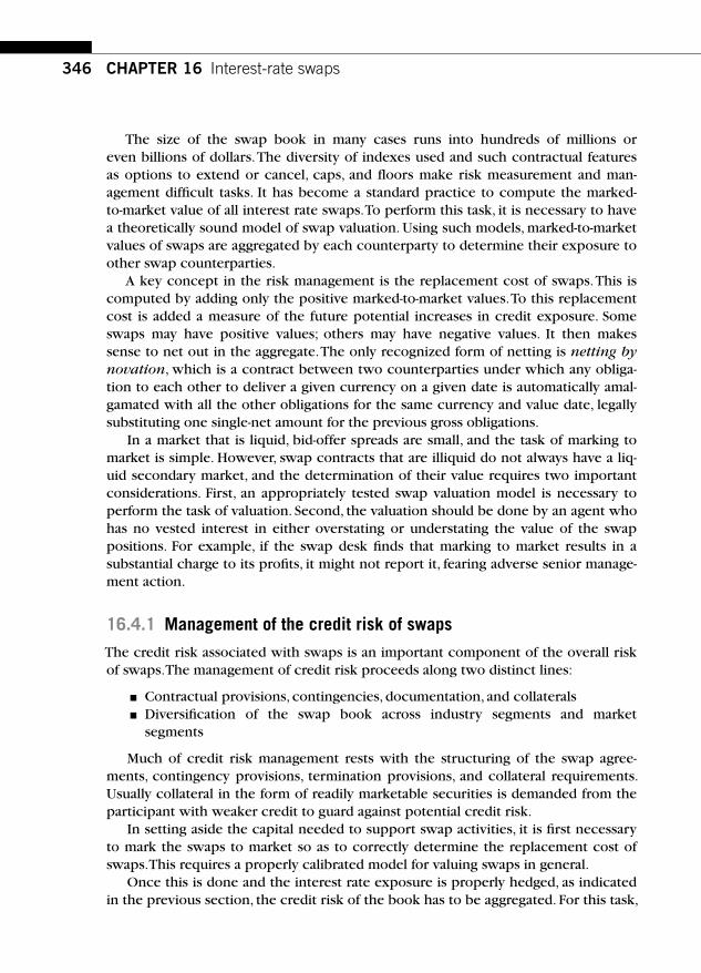
346 CHAPTER 16 Interest-rate swaps
The size of the swap book in many cases runs into hundreds of millions or even billions of dollars. The diversity of indexes used and such contractual features as options to extend or cancel, caps, and fl oors make risk measurement and man-agement diffi cult tasks. It has become a standard practice to compute the marked-to-market value of all interest rate swaps. To perform this task, it is necessary to have a theoretically sound model of swap valuation. Using such models, marked-to-market values of swaps are aggregated by each counterparty to determine their exposure to other swap counterparties.
A key concept in the risk management is the replacement cost of swaps. This is computed by adding only the positive marked-to-market values. To this replacement cost is added a measure of the future potential increases in credit exposure. Some swaps may have positive values; others may have negative values. It then makes sense to net out in the aggregate. The only recognized form of netting is netting by novation, which is a contract between two counterparties under which any obliga-tion to each other to deliver a given currency on a given date is automatically amal-gamated with all the other obligations for the same currency and value date, legally substituting one single-net amount for the previous gross obligations.
In a market that is liquid, bid-offer spreads are small, and the task of marking to market is simple. However, swap contracts that are illiquid do not always have a liq-uid secondary market, and the determination of their value requires two important considerations. First, an appropriately tested swap valuation model is necessary to perform the task of valuation. Second, the valuation should be done by an agent who has no vested interest in either overstating or understating the value of the swap positions. For example, if the swap desk fi nds that marking to market results in a substantial charge to its profi ts, it might not report it, fearing adverse senior manage-ment action.
16.4.1 Management of the credit risk of swaps
The credit risk associated with swaps is an important component of the overall risk of swaps. The management of credit risk proceeds along two distinct lines:
■ Contractual provisions, contingencies, documentation, and collaterals ■ Diversifi cation of the swap book across industry segments and market
segments
Much of credit risk management rests with the structuring of the swap agree-ments, contingency provisions, termination provisions, and collateral requirements. Usually collateral in the form of readily marketable securities is demanded from the participant with weaker credit to guard against potential credit risk.
In setting aside the capital needed to support swap activities, it is fi rst necessary to mark the swaps to market so as to correctly determine the replacement cost of swaps. This requires a properly calibrated model for valuing swaps in general.
Once this is done and the interest rate exposure is properly hedged, as indicated in the previous section, the credit risk of the book has to be aggregated. For this task,

347
it is useful to subdivide the swaps into two groups: one in which the intermediary is paying fi xed and the other in which the intermediary is paying fl oating. Within each of these groups, swaps must be further classifi ed across various credit risk categories and then marked to market and aggregated within those credit risk classifi cations. This will enable the management of the swap book to identify which of the swap agreements have signifi cant replacement costs due to deteriorating credit risk and to what extent the swap book is reasonably matched. Marking to market will effectively indicate the health of the swap book on termination of each swap agreement (vol-untary or involuntary) in the book. If there is a net loss, the capital set aside should be suffi cient to meet those losses.
16.5 SWAP BID RATE, OFFER RATE, AND BID-OFFER SPREADS As the swap dealer’s credit reputation deteriorates, two important changes tend to occur. First, the bid-offer spread will decrease. This is because the counterparties recognize the fact that a swap dealer with a lower credit reputation will play the role of clearinghouse less effectively. Second, the dealer will start to lose counterpar-ties of good credit reputation and start to attract counterparties of lower credit repu-tation. This effect may counterbalance the previous effect.
The empirical evidence on swap bid-offer spreads suggests that swap dealers with better credit reputation enjoy much higher bid-offer spreads.
Sun, Sundaresan, and Wang (1993) examine the effect of the dealer’s credit repu-tation on the bid-offer spreads of swap quotations. They show that the swap bid-offer spreads for AAA dealers were nearly twice the swap bid-offer spreads of A dealers.
Assume that the credit quality of the counterparties is the same for different swap dealers and that the swap contracts do not differ in other dimensions, such as the up-front fee and collaterals. Then, intuitively, the swap-offer rates of AAA-rated dealers should be higher than those of A-rated dealers, whereas the swap-bid rates of AAA-rated dealers should be lower than those of A-rated dealers. (See Figure 16.1 . AAA-rated dealers should be able to collect higher rents by increasing the swap bid-offer spreads.)
Most swap dealers offer swap quotations that are the same irrespective of the credit standing of clients. Usually, an up-front fee is assessed, depending on the matu-rity and the notional amount of the swap contract. This fee might vary with the credit standing of clients. Marking to market and the posting of marketable collateral may be required of clients whose credit quality declines with time. Clearly, these pro-visions are integral parts of swap contracts.
In this context, it is useful to note that swap dealers tend to work with an approved list of clients who have been cleared by the swap dealer’s credit commit-tee. For example, the AAA dealer may require that the average credit rating of any counterparties be AA or better; the minimum acceptable credit rating is A. In this case, it seems reasonable to assume that the credit quality of the counterparties is relatively better for the AAA dealer, which will counteract the AAA dealer’s advantage
16.5 Swap bid rate, offer rate, and bid-offer spreads

348 CHAPTER 16 Interest-rate swaps
in charging higher bid-offer spreads. Hence, the empirical fi nding that the AAA swap rates bracket the A swap rates lends stronger support to our hypothesis about the impact of credit ratings on bid-offer spreads.
Credit risk of parties involved in swaps infl uences the swap bid rate and offer rates. Swap offer and bid rates must be bounded by two reference rates. The swap offer rate should be lower than the par bond yield of the counterparty to the dealer. If the swap offer rate (say, 7%) is higher than the counterparty’s par bond yield (say, 6.5%) the counterparty can do the following: He can issue a par bond and invest the proceeds in LIBOR (we ignore bid-offer spread). He will get 6.5% � LIBOR, which is better than what he will get on the offer side. The swap bid rate should be lower than the par bond yield of the dealer. If the swap bid rate (say, 6.75%) is lower than dealer’s par bond yield (say, 6.5%), the dealer can do the following: He can issue a par bond and invest the proceeds in LIBOR (we ignore bid-offer spread). He will pay 6.5% and get LIBOR. This is better than what he will get on the bid side. (See Figure 16.1 to better understand these transactions.)
To prevent arbitrage, the swap bid rate should be lower than the par bond yield of the counterparty to the dealer on the offer side. If the swap bid rate (say, 7%) is higher than the counterparty’s par bond yield (say, 6.5%), the dealer can do the fol-lowing: She can issue a par bond and invest the proceeds in LIBOR (we ignore bid-offer spread). She will get 6.5% � LIBOR. She can then hit the bid of the swap, which will pay her 7% and require only LIBOR, which is already funded.
16.6 SWAPTIONS Options that give the right to enter into a swap at a future date at terms that are agreed on now are known as swaptions. Payer swaptions give the right but not the obligation to pay the fi xed rate and receive the fl oating payments on a swap of spec-ifi ed tenor. Receiver swaptions give the right but not the obligation to receive the fi xed rate and pay the fl oating payments on a swap of specifi ed tenor. These particu-larly valuable instruments hedge a stream of contingent future cash fl ows.
Example 16.5 Let’s say that a company has bid for a project. If the company wins the bid, the project will produce a stream of 5 million FX per year over the next 10 years. Let’s say that the results of the bid will be known in three months.
The company can enter into a payer swaption with a three-month maturity, which gives the right to pay 5 million FX per year and receive LIBOR. If the company wins the bid, the swap-tion will be exercised at maturity, and the FX exposure would be swapped to LIBOR. If the company loses the bid, the swaption can be sold or allowed to expire.

349
Example 16.6 Consider a fi xed income portfolio manager who has a callable bond at a coupon of 10%. Yields are falling, and there is a possibility that the bond may be called. Let’s say that the call price is 100. The bond’s fi rst call date is 6 months from now, and the bond has 10 years more to maturity from the fi rst call date. How can the portfolio manager hedge the call risk?
The portfolio manager can buy a receiver swaption with six months ’ maturity on an inter-est rate swap with a maturity of 10 years. The interest rate swap will pay a fi xed rate equal to the coupon of the callable bond. In exchange, the portfolio manager will have to pay LIBOR. Suppose that the interest rates drop, and the bond gets called at the end of six months. Then the portfolio manager will exercise the swaption and receive the coupon as though he still owned the bond. However, he has to pay LIBOR now. This can be done by investing the call price (which he would have received when the bond was called) in LIBOR. This way the call can be stripped from callable bonds.
Figure 16.11 considers a situation where the swaption is available for trading on T � 0. The maturity date of the swaption is T � 1, and the underlying interest rate swap has a maturity of fi ve years. Assume for simplicity that the swap pays fi xed coupons every year in return for LIBOR. Assume that the strike rate of the swaption is a fi xed rate x .
At T � 1, we can engage in a swap. This swap rate, y, is the par bond yield at T � 1. If instead we can buy a swaption at T � 0 at a rate x, its value at T � 1 is the value of a bond that has a coupon rate of x. Consider a swaption on a generic fi ve-year swap so that the reset date precedes the payment date by exactly the index maturity. Let’s denote the discount factors for discounting cash fl ows that occur i years later by di. Therefore, d 2 will be the zero coupon bond price at T � 1 for discounting the cash fl ows that will occur two years after T � 1.
The value of a swap on T � 1 that pays y:
y d d d d d d1 2 3 4 5 51 0� � � � � � �⎡⎣ ⎤⎦ ⎡⎣ ⎤⎦ . (16.6)
This is because y is the par bond yield. The value of a swap on T � 1 that pays x would be
x d d d d d d1 2 3 4 5 51 0� � � � � � �⎡⎣ ⎤⎦ ⎡⎣ ⎤⎦ .
16.6 Swaptions
T�0 T�1
FIGURE 16.11
Swaption Start Date and Maturity Date

350 CHAPTER 16 Interest-rate swaps
Obviously, the holder of a payer swaption will exercise if
x d d d d d d1 2 3 4 5 51 0� � � � � � �⎡⎣ ⎤⎦ ⎡⎣ ⎤⎦ .
or
x d d d d d d1 2 3 4 5 51 1� � � � � �⎡⎣ ⎤⎦ .
The owner of this swaption will get payoffs, which may be represented by the equation
max , .0 1 11 2 3 4 5 5− + + + +⎡⎣ ⎤⎦ +{ }⎡⎣⎢
⎤⎦⎥x d d d d d d
This is an option to sell a fi ve-year bond paying a coupon of x at par. We can therefore value swaptions as options to sell or buy bonds at a strike price of par.Any bond options pricing model is then a good way to value swaptions. Investors also use Black’s model on options on futures to value swaptions. They use the for-ward swap rate as an input into Black’s model.
Let C � payer swaption, P � receiver swaption, s � tenor of the swap, F � for-ward swap rate on the swap, K � strike rate on the swaption, r � fi nancing rate, T � t � time to maturity, and m � number of compounding per year in swap rate, and σ is the volatility of the forward swap rate. Then the value of the swaption can be found using the following modifi ed Black’s model:
C e FN d KN d
F
m
Fr T t
s m
� � �
�
�� �
�
( ) ( ) ( ) .1 2
11
1
[ ]
⎛⎝⎜⎜⎜
⎞⎠⎟⎟⎟
(16.7)
P e KN d FN d
F
m
Fr T t
s m
� � � � �
�
�� �
�
( ) ( ) ( ) .21 1
11
1
[ ]
⎛⎝⎜⎜⎜
⎞⎠⎟⎟⎟
(16.8)
Example 16.7 Let’s value a two-year payer swaption on a four-year swap with semiannual compounding. Assume a notional principal of $10 million. The forward swap rate on a four-year swap is 7% when it starts two years from now. The strike rate is 7.5%, and the fi nancing rate is 6%. The volatility of the forward swap rate is 20%.

351
We apply Black’s formula with semiannual compounding ( m � 2) in Table 16.13 . The payer swaption is a call option and the receiver swaption is a put option.
16.6 Swaptions
Table 16.13 Swaption Valuation
Table 16.14 Parity for Swaptions
t � 0 x � Swap Rate x � � Swap Rate
t � 1 t � 2 t � 3 t � 4 t � 1 t � 2 t � 3 t � 4
1. Enter into a
forward swap at a
forward rate of x
x-LIBOR x-LIBOR x-LIBOR x-LIBOR x-LIBOR x-LIBOR x-LIBOR x-LIBOR
2. Buy a receiver
swaption
x-LIBOR x-LIBOR x-LIBOR x-LIBOR 0 0 0 0
3. Sell a payer
swaption
0 0 0 0 x-LIBOR x-LIBOR x-LIBOR x-LIBOR
Hence, it follows that a forward swap is a portfolio of a long position in a receiver swaption and a short position in a payer swaption.
16.6.1 Swaption parity relation
There is a parity relation among the values of (a) payer swaption, (b) receiver swap-tion, and (c) forward swap rate. To see the parity condition, let’s examine the payoffs associated with the transactions shown in Table 16.14 .
Since a receiver swaption is a put on a bond with a strike of par and a payer swaption is a call on the same bond with a strike of par, we can apply the put-call parity to get the same implication. Table 16.15 shows the put-call parity. It shows that a long position in a put on a bond coupled with a short position in a call repli-cates a forward swap.

352 CHAPTER 16 Interest-rate swaps
16.7 CONCLUSION We showed several ways that interest rate swaps are priced. Eurodollar futures pro-vide one avenue. Another avenue is to extract the zero prices from the market and work with them. We showed that the spreads between swap rates and Treasury yields, overall, increase signifi cantly with maturities, whereas the increase is much smaller when the Treasury yield curve is inverted. The bid-offer spreads of market makers are sensitive to their credit reputations. It is interesting to note that Merrill Lynch and several other fi rms have formed new subsidiaries to engage in the swap business with large clients; these separately capitalized, credit-enhanced subsidiaries have been structured to get an AAA rating. Several other investment banks, including Salomon Brothers, have launched such credit-enhanced subsidiaries. In the equity derivatives market, a self-funded AAA vehicle has been formed by Goldman Sachs.
SUGGESTED READINGS AND REFERENCES Bicksler , J. , & Chen , A. H. ( 1986) . An economic analysis of interest rate swaps . Journal of Finance ,
41 , 645 – 655 .
Capital adequacy: The BIS framework and its portfolio implications. The Journal of International Securities Markets , 191 –218.
Cooper , I. , & Mello , A. S. ( 1991) . The default risk of swaps . Journal of Finance , 48 , 597 – 620 .
Federal Reserve System. (1987). Capital maintenance: Revision to capital adequacy guidelines. Regulation Y: Docket No. R-0567.
Ramaswamy , K. , & Sundaresan , S. M. ( 1986) .The valuation of fl oating-rate instruments: Theory and evidence . Journal of Financial Economics , 17 , 251 – 272 .
Smith , C. W. , Smithson , C. W. , & Wakeman , L. M. ( 1988) . The market for interest rate swaps . Financial Management , 17 , 34 – 44 .
Sun , T. , Sundaresan , S., & Wang , C. ( 1993) . Interest rate swaps: An empirical investigation . Journal of Financial Economics , 36 , 77 – 99 .
Sundaresan , S. M. ( 1991) . Valuation of swaps . In S. J. Khoury (Ed.), Recent developments in interna-tional banking and fi nance (Vol. 5 ) . Elsevier Science Publishers .
Table 16.15 Parity for Swaptions
t � 0 x � Swap Rate at Option’s Maturity
x � � Swap Rate at Option’s Maturity
1. Buy a put option on a bond paying a coupon rate of x
0 1 11 3 3 4� � � � �x d d d d[ ]
2. Sell a call on a bond paying a coupon rate of x
1 11 3 3 4� � � � �x d d d d[ ] 0
Buying a put and selling a call on a bond replicates a forward swap.

353
CHAPTER
CHAPTER SUMMARY This chapter defi nes forward contracts and futures contracts. Differences between forwards and futures are then explained. Treasury futures contracts are then described and analyzed. The delivery options in Treasury (note and bond) futures contracts and their implications for delivery strategies and pricing are explained using concrete examples. Concepts such as basis, basis after carry (net basis), value of delivery options, and implied repo rate are explained with examples. We show how Treasury futures contracts can be used in hedging and risk management applications.
17.1 FORWARD CONTRACTS DEFINED An investor who buys (sells) a forward contract agrees to buy (sell) one unit of the underlying asset at a specifi ed future time, called the maturity date. The price at which the purchase will be made is called the forward price. The forward price is determined when the contract is written; it is specifi ed in the contract and does not change over the life of the contract. An investor who has agreed to buy is said to be long in the forward market, and the investor who has agreed to sell is said to be short in the forward market. The forward price is chosen so that the purchaser of the forward contract, the long position, pays and receives nothing when the contract is written. At the time of maturity, the long position receives one unit of the asset or its cash value, which is delivered by the seller of the forward contract, the short posi-tion. On the maturity date, the short position receives the forward price specifi ed in the contract.
Treasury futures contracts 17
Fixed Income Markets and Their DerivativesCopyright 2009 by Academic Press. Inc. All rights of reproduction in any form reserved.
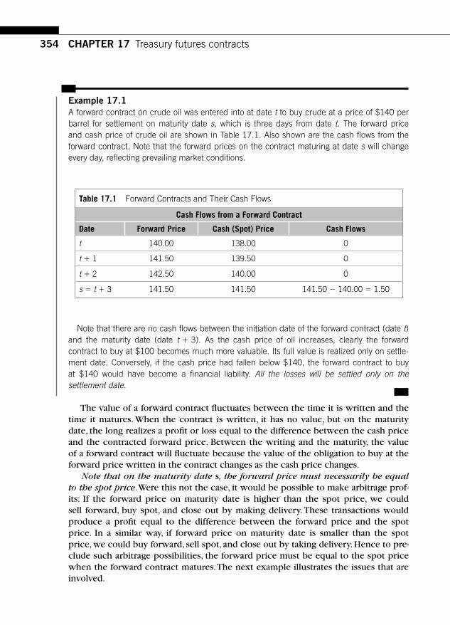
354 CHAPTER 17 Treasury futures contracts
Example 17.1 A forward contract on crude oil was entered into at date t to buy crude at a price of $140 per barrel for settlement on maturity date s, which is three days from date t. The forward price and cash price of crude oil are shown in Table 17.1 . Also shown are the cash fl ows from the forward contract. Note that the forward prices on the contract maturing at date s will change every day, refl ecting prevailing market conditions.
Table 17.1 Forward Contracts and Their Cash Flows
Cash Flows from a Forward Contract
Date Forward Price Cash (Spot) Price Cash Flows
t 140.00 138.00 0
t � 1 141.50 139.50 0
t � 2 142.50 140.00 0
s � t � 3 141.50 141.50 141.50 � 140.00 � 1.50
Note that there are no cash fl ows between the initiation date of the forward contract (date t ) and the maturity date (date t � 3). As the cash price of oil increases, clearly the forward contract to buy at $100 becomes much more valuable. Its full value is realized only on settle-ment date. Conversely, if the cash price had fallen below $140, the forward contract to buy at $140 would have become a fi nancial liability. All the losses will be settled only on the settlement date.
The value of a forward contract fl uctuates between the time it is written and the time it matures. When the contract is written, it has no value, but on the maturity date, the long realizes a profi t or loss equal to the difference between the cash price and the contracted forward price. Between the writing and the maturity, the value of a forward contract will fl uctuate because the value of the obligation to buy at the forward price written in the contract changes as the cash price changes.
Note that on the maturity date s , the forward price must necessarily be equal to the spot price. Were this not the case, it would be possible to make arbitrage prof-its: If the forward price on maturity date is higher than the spot price, we could sell forward, buy spot, and close out by making delivery. These transactions would produce a profi t equal to the difference between the forward price and the spot price. In a similar way, if forward price on maturity date is smaller than the spot price, we could buy forward, sell spot, and close out by taking delivery. Hence to pre-clude such arbitrage possibilities, the forward price must be equal to the spot price when the forward contract matures. The next example illustrates the issues that are involved.

355
Example 17.2 On March 12, XYZ Corporation agrees to buy 1000 barrels of crude oil from West Texas Intermediate (WTI) at a price of $140 per barrel with the understanding that the crude oil will be delivered to Cushing, Oklahoma, on May 12, a period of 60 calendar days from March 12. Assume that the fi nancing costs amount to 8.0% annualized. If, 30 days later, the crude oil forward price is quoted at $137 per barrel for a forward contract expiring in 30 days, what is the value of the forward contract to XYZ Corporation?
It should be clear that XYZ Corporation has a forward contract (at a forward price of $140) with a negative value. XYZ can dispose of it only by paying compensation to a third party. This can be accomplished by selling forward at a forward price of $137 on April 12. At maturity date, the physical delivery of oil from the original forward contract is used to cover the short position in the second forward contract that was established on April 12. The loss on May 12 is ($140 � $137) � 1000 � $3000. The present value of the contract as of April 12 is
3000
10 08 30
360
2980 13�
��
.. .
⎛⎝⎜⎜⎜
⎞⎠⎟⎟⎟⎟
The fl uctuation in the value of a forward contract is due to the fact that forward contracts are not marked to market; namely, gains and losses are settled each day by the counterparties to the contract. The futures contracts, which we describe next, are marked to market daily, and their value after they are marked to market is always zero.
17.2 FUTURES CONTRACTS DEFINED An investor who takes a long (short) position in a futures contract agrees to buy (sell) specifi ed units of the underlying asset (or its cash value) on a specifi ed matu-rity date at a currently specifi ed futures price. The futures price is determined when the contract is written and is specifi ed in the contract. The futures price is set so that no payment is made when the contract is written; that is, at initiation, the futures contract has a zero market value. As the contract matures, however, the investor must make or receive daily installment payments toward the eventual purchase of the underlying asset. The total of the daily installments and the payment at matu-rity will equal the futures price set when the contract was initiated.
The daily installments are determined by the daily change in the futures price. Ifthe futures price goes up, the investor who is long in the futures contract receives a payment from the investor who is short that equals the change in the daily futures price. This process is called marking to market on futures exchanges.
The effect of marking to market is to rewrite the futures contract each day at the new futures price. Hence the value of the futures contract after the daily settle-ment will always be zero, since the value of a newly written futures contract is zero. When the contract matures, the long will have already paid or received the difference
17.2 Futures contracts defi ned

356 CHAPTER 17 Treasury futures contracts
between the initial futures price and the futures price at the maturity time. With these payments to her credit, she will have a balance due equal to the futures price at the maturity time. However, the value of a futures contract written at the maturity time for immediate delivery must be zero. Therefore, at maturity, the futures price must equal the current spot price: The balance due is simply the current spot price at the maturity time.
Table 17.2 presents the cash fl ows from the long position in a futures contract. Note that the sum of the cash fl ows in the last column of Table 17.2 is simply the difference between the spot price at maturity and the contracted futures price at date t. In our example, the cumulative mark-to-market cash fl ows equal $1.50. When deducted from the spot price of $141.50, this yields $140.00, which is the con-tracted futures price at date t.
Recall that at maturity date s of a futures contract, the futures price must be exactly equal to the cash price. This means that if the futures price is higher than the cash price at maturity and the investor sells futures and buys cash and effects delivery, the investor can make riskless profi ts. Similarly, if the futures price is less than the cash price and the investor buys futures and sells cash, the investor can make riskless profi ts.
Exceptions to the rule that the futures price must equal the cash price occur whenever the futures contracts provide either the short or the long with some deliv-ery options. These exceptions are fully treated in the context of specifi c futures mar-kets later.
The holder of a futures position receives or pays cash on a daily basis. An inves-tor with a long (short) position receives (pays) cash fl ows when the futures prices increase and pays (receives) cash fl ows when the futures prices fall. If the future inter-est rates are random, this introduces a reinvestment risk. If cash is fully invested in interest-bearing securities, a margin call resulting from unfavorable changes in futures prices will force the investor to liquidate some of the assets to post the additional mar-gin. The opportunity cost of this is unknown at the time the futures position was initi-ated. Similarly, any receipts of cash due to favorable changes in futures prices will have to be reinvested at rates unknown at time t. As a result, we may expect the futures prices at time t to not only embody the expectations about the future cash price at time s but also the path of one-period interest rates between time t and time s.
Table 17.2 Futures Contracts and Their Cash Flows
Cash Flows from a Futures Contract
Date Futures Price Cash (Spot) Price Cash Flows
t 140.00 138.00 0
t � 1 141.50 139.50 1.50
t � 2 142.50 140.00 1.00
s � t � 3 141.50 141.50 � 1.00
357
17.3 DESIGN OF CONTRACTUAL FEATURES The defi nition of the futures contract and the discussion of the contracts presented here capture the essential features of futures contracts. However, several real-life fea-tures of such contracts must be considered.
17.3.1 Delivery specifi cations
The exchanges must decide whether the futures contract calls for physical delivery or cash settlement. In contracts that specify delivery, the seller of the futures con-tract must deliver the underlying asset on the maturity date if his short position is not already closed out. In contracts that specify cash settlement, the seller of futures need not deliver and the contract is settled in cash. In addition, the exchanges must decide on the set of assets that investors can use to satisfy the delivery requirements. The delivery parameters, such as location, timing, and quality, have to be specifi ed in detail; these issues are resolved on a case-by-case basis. There are also some common considerations that underlie the choice of delivery specifi cations.
First, the delivery specifi cations must be such that the deliverable assets are in competitive supply so that no single economic agent acting alone or a group of dominant agents acting in collusion will be able to corner the supply of deliverable assets. The principal implication of this is the design requirement that, in the case of commodity futures contracts, the deliverable set includes several grades of com-modities. For futures contracts on fi nancial assets, such as Treasury bonds or Treasury notes, many bonds and notes issued by the Treasury qualify for delivery. Though such a design feature mitigates the problem of corners, it introduces a different problem: With so many deliverable assets, the maturity futures price will tend to track the price of cheapest deliverable asset. This is due to the fact that the seller of futures contract, acting rationally, will deliver the cheapest of the deliverable assets.
At the time of contracting, however, investors do not know which asset will be the cheapest when the contract expires. This introduces another element of uncer-tainty. Exchanges have attempted to deal with this problem by standardizing the assets that may be delivered against a futures contract. For example, in the case of T-bond futures contracts, the Chicago Board of Trade (CBOT) has stipulated that the standard grade is the 6%, 20-year bond issued by the Treasury. The deliverable set, however, includes all the bonds issued by the Treasury that have 15 years or more to fi rst call date or maturity. CBOT then standardizes these bonds through a system of conversion factors that attempt to equalize the attractiveness of delivering any of the deliverable assets. These issues are taken up for detailed analysis later.
It is worth noting that only a tiny percentage of futures contracts are closed by physical delivery, and most of them are offset prior to the maturity date. An offset occurs when an investor who is short in a futures contract takes an equal amount of long position in the same futures contract and closes out his position. This should come as no surprise, since the diversity of deliverable grades makes taking physical delivery less attractive.
17.3 Design of contractual features

358 CHAPTER 17 Treasury futures contracts
Table 17.3 records the proportion of mature open interest that is settled by physi-cal delivery. Note that the maximum amount of open interest that is settled by physi-cal delivery is 6.3%. The Chicago Board of Trade (CBOT) defi nes mature open interest in an expiring futures contract as the median level of daily open interest in the con-tract during the 42-business-day interval ending on the contract’s fi rst position day, which is the fi rst day in the process of making or taking delivery of the actual com-modity on a future.
A further reduction in incentive to take delivery is attributable to the fact that the short can make delivery on any business day of the delivery month, typically with a short notice period. This fl exibility is called the timing option implicit in futures contracts. Many futures contracts permit the short some fl exibility in the choice of the location of physical delivery as well. This is referred to as the location option embedded in futures contracts.
17.3.2 Price limits
The exchanges may impose price limits. These limits stipulate the range of futures prices within which trading will be sustained in the futures markets. When the futures prices reach the limit, the investor is locked into her position and cannot offset. Typically, the limits are removed during the delivery months of the futures contract.
17.3.3 Margins
Exchanges set margins to ensure that the investor has suffi cient equity to meet any adverse price moves. This, in conjunction with marking to market and price limits, minimizes the risk of nonperformance by investors who take futures positions. In much of the analysis in this book, we assume that the initial margin requirements to open a futures position can be met by posting interest-bearing securities. This turns out to be a realistic assumption, although in some instances a small percentage of
Table 17.3 Treasury Futures Deliveries, December 1996 –December 2006 (Median Values)
Contract Physical Deliveries as Percentage of Mature
Open Interest
Open Interest on First Position Day as Percentage of Mature
Open Interest
T-bond 2.2% 47%
10-year T-note 2.7% 46%
5-year T-note 3.7% 49%
2-year T-note 6.3% 51%
Sources: Chicago Board of Trade and Commodity Futures Trading Commission.

359
the margin will have to be posted in cash. Once the initial margin level falls to a pre-specifi ed level, called the maintenance margin, margin calls will result. This usually happens when the futures prices move in an adverse manner relative to the estab-lished futures position for several consecutive days. When this happens, the investor must restore the margin level to the initial margin level by posting cash.
17.4 FUTURES VERSUS FORWARDS In sum, forward contracts differ from futures contracts in a number of ways. Forwards are not marked to market, as futures contracts are. This alone is suffi cient to cause a difference in the forward prices and futures prices in the presence of inter-est rate uncertainty. Institutions, either on a bilateral basis, as in the case of the oil industry, or through extensive OTC markets, as in the case of foreign currency mar-kets, typically enter into forwards. Futures contracts, on the other hand, are traded in centralized open outcry exchanges in which bid-offer prices are established. The difference in the market organization, in turn, requires different institutional arrange-ments for ensuring performance. In the futures markets, anyone with a reasonable amount of capital can participate. Exchanges have clearinghouses that monitor the performance of participants through the system of marking to market, margins, and margin calls that force the participants to respond quickly to adverse price move-ments. If any investor is unable to respond, that investor’s open position is corre-spondingly reduced and ultimately extinguished. The clearinghouses have capital that they can rely on to meet any residual shortfall. This mechanism is necessary for the open outcry markets to function; there is no time in such a market to conduct extensive credit checks on investors. In forward markets, the situation is quite differ-ent. In the bilateral contracts prevalent in the oil industry, for example, the corpora-tions receive suffi cient information about the credit risk that they face in forward contracting. This enables them to design the necessary contractual terms (such as collateral, for example) to protect themselves from any nonperformance contingen-cies. In OTC forward markets, high capital requirements and collateral requirements are enforced to screen investors with high credit risk. Forward contracts, especially the ones in bilateral settings, specify precise terms concerning the deliverable grades, location, and delivery dates. The goal in such a contracting process is delivery. As such, forward contracts are often more customized. This aspect differs sharply from the delivery specifi cations of futures contracts, which are standardized with specifi c maturity months and which provide the short with the many embedded options we discussed previously.
17.5 TREASURY FUTURES CONTRACTS A considerable increase in the volatility in interest rates occurred after the shift in the Fed’s monetary policy in October 1979. In Chapter 3 we examined this shift and
17.5 Treasury futures contracts

360 CHAPTER 17 Treasury futures contracts
documented the increased volatility in interest rates that accompanied that shift. The interest rates have continued to fl uctuate a great deal since that shift. This increased volatility has posed signifi cant risks for issuers, fi nancial intermediaries, and investors.
To successfully manage such risks, it is necessary to have hedging vehicles in the marketplace. The introduction of Treasury bond futures contracts in the CBOT in August 1977, Treasury note (10-year) futures contracts in the CBOT in 1982, and the introduction of Treasury note (5-year) futures contracts in CBOT are, in part, a response to these factors. This section describes the specifi cations of Treasury futures contracts. T-bond futures contracts and their specifi cations are analyzed in detail. Since the Treasury note futures are similar to Treasury bond futures, the analy-sis for the Treasury bond futures applies to the note contracts as well.
The salient features of the T-bond futures contract are provided next. In Table 17.4 , contractual provisions for Treasury bond futures are indicated. The T-bond futures contract and its design has been extensively copied and adopted by a num-ber of exchanges. The gilt futures contract at LIFFE, the French government bond contract at MATIF, the Bund futures contract on the German government bond, and the Japanese government bond contract have extensively used the design specifi ca-tions of U.S. T-bond futures contract traded at CBOT.
Table 17.5 presents the contractual specifi cations for the 10-year T-note futures contracts. Both T-bond and T-note futures contracts are actively traded instruments. For example, in July the open interest in 10-year T-note futures stood at 1.87 million contracts, each with a par value of $100,000. For T-bond futures, the corresponding fi gure was 896,000 contracts.
Both T-notes and T-bonds are delivered via the Fed wire system. In 2000, CBOT set the deliverable grade to a 6% standard. Prior to the March 2000 contract, the delivery standard was 8%. This change was effected due to a steep drop in long-term yields.
17.5.1 Delivery options in treasury note futures
It is important to fully understand the T-note futures contract specifi cation, to deter-mine the relationship between futures prices and Treasury note prices. A seller of a T-note futures contract has a great deal of fl exibility or many delivery options during the delivery month.
The short may deliver any bundle of prespecifi ed Treasury notes sometime dur-ing the delivery month so long as the investor has not offset her short position. This is referred to as the quality option. This is perhaps the most important option in the T-note futures contract.
The Treasury note futures contract closes for the day at 2:00 p.m. Chicago time. The Treasury note market, however, is a dealers ’ market. Indeed, as long as bond deal-ers are willing to execute orders, the bond market may be considered open. The clearinghouse of the CBOT accepts delivery during the delivery month until 8:00 p.m. Chicago time. These observations mean that an investor who has an open short position in T-bond futures as of 2:00 p.m. Chicago time during the delivery month has the option to deliver any combination of the deliverable issues until 8:00 p.m.

361
Chicago time. If the deliverable issues were to experience a signifi cant price decline during the 2:00 p.m. to 8:00 p.m. period, this option will be of considerable value to the investor who is short. This option is known as the wildcard delivery option in T-note futures contracts. The key is that the invoice price is fi xed at 2:00 p.m. and does not change until the next day of trading. The investor may elect to delay deliv-ery by waiting. This strategy permits the investor to participate in any potential price declines in the 2:00 – 8:00 p.m. period next day.
In essence, the investor who is short on the fi rst day of the delivery month has a sequence of six-hour put options during each day of the delivery month until the
17.5 Treasury futures contracts
Table 17.4 T-Bond Futures Contract Specifi cations
Contract size One U.S. Treasury bond having a face value at maturity of $100,000, or multiple thereof
Deliverable grade U.S. Treasury bonds that, if callable, are not callable for at least 15 years from the fi rst day of the delivery month or, if not callable, have a maturity of at least 15 years from the fi rst day of the delivery month
Conversion factor The conversion factor is the price of the delivered bond ($1 par value) to yield 6%
Invoice price The invoice price equals the futures settlement price times a conversion factor plus accrued interest
Tick size Minimum price fl uctuations shall be in multiples of 1/32nd point per 100 points ($31.25 per contract), except for intermonth spreads, where minimum price fl uctuations shall be in multiples of 1/4 of 1/32nd point per 100 points ($7.8125 per contract); par shall be on the basis of 100 points, and contracts shall not be made on any other price basis
Price quote Points ($1000) and 32nds of a point; for example, 80-16 equals 80-16/32
Contract months March, June, September, December
Last trading day Seventh business day preceding the last business day of the delivery month; trading in expiring contracts closes at noon, Chicago time, on the last trading day
Last delivery day Last business day of the delivery month
Trading hours Open auction: 7:20 a.m. – 2:00 p.m., Chicago time, Monday – Friday
Electronic: 6:00 a.m. – 4:00 p.m., Chicago time, Sunday –Friday
Trading in expiring contracts closes at noon, Chicago time, on the last trading day
Ticker symbols Open auction: US
Electronic: ZB
Source: Chicago Board of Trade.

362 CHAPTER 17 Treasury futures contracts
last day of futures trading. Each put provides the right to sell a bundle of deliverable issues until 8:00 p.m. at an invoice price set at 2:00 p.m. Upon expiration, the inves-tor gets another put at a different invoice (strike) price the next day at 2:00 p.m. The T-note futures cease trading seven business days prior to the last business day of the contract month. Thus the wildcard option provides the short with a sequence of approximately 15 daily put options. It is easy to see the directional impact of the wildcard option on T-bond futures price. Since the short has the fl exibility associated with the wildcard feature, the long will enter into the futures transaction only if the futures price is discounted by the value of the sequence of put options represented by the wildcard feature. Thus, the effect of a wildcard option, in a rational setting, is to reduce the futures price by the fair value of the option.
Table 17.5 Ten-Year T-Note Futures Contract Specifi cations
Contract size One U.S. Treasury note having a face value at maturity of $100,000, or multiple thereof
Deliverable grade U.S. Treasury notes maturing at least 6.5 years but not more than 10 years from the fi rst day of the delivery month
Conversion factor The conversion factor is the price of the delivered bond ($1 par value) to yield 6%
Invoice price The invoice price equals the futures settlement price times a conversion factor plus accrued interest
Tick size Minimum price fl uctuations shall be in multiples of 1/32nd point per 100 points ($15.625 per contract), except for intermonth spreads, where minimum price fl uctuations shall be in multiples of 1/4 of 1/32nd point per 100 points ($7.8125 per contract); par shall be on the basis of 100 points, and contracts shall not be made on any other price basis
Price quote Points ($1000) and 32nds of a point; for example, 80-16 equals 80-16/32
Contract months March, June, September, December
Last trading day Seventh business day preceding the last business day of the delivery month; trading in expiring contracts closes at noon, Chicago time, on the last trading day
Last delivery day Last business day of the delivery month
Trading hours Open auction: 7:20 a.m. –2:00 p.m., Chicago time, Monday –Friday
Electronic: 6:00 a.m. –4:00 p.m., Chicago time, Sunday –Friday
Trading in expiring contracts closes at noon, Chicago time, on the last trading day
Ticker symbols Open auction: TY
Electronic: ZN
Source: Chicago Board of Trade.

363
The T-note futures contract ceases trading seven business days prior to the last business day of the contract month. The clearinghouse, however, accepts delivery until the last business day of the month. Between the last day of futures trading and the last delivery date, note prices fl uctuate in the marketplace, but the futures price stays fi xed at its closing level as of the last trading day. This feature of the Treasury note futures contract is called the end-of-the-month option. The holder of a short position in Treasury note futures has considerable fl exibility during this period. He has a timing option that permits him to select any day during this period to make delivery. Furthermore, holders have a quality option that permits them to select any bundle of deliverable notes from among the eligible deliverable issues.
Note that the design of a T-note futures contract provides several implicit options to the short. This is typical of many futures contracts, as we have seen. These delivery options have important effects on the relationship between futures prices and cash prices.
T-note and T-bond futures contracts are traded in quarterly maturity cycles as shown in Table 17.6 .
At any time only the next two quarterly maturities have any liquidity. The near-est maturity contract obviously enjoys a great deal of liquidity until it is close to the expiration date.
17.5.2 Conversion factor
A key concept associated with the Treasury futures contract is the concept of a con-version factor. We analyze this concept in the context of a specifi c T-note futures contract that expired in September 2007. The settlement date for this contract was September 5, 2007. The September 2007 futures price was at 109.484 (in decimals). The fi nancing rate (repo) was 4.83%.
A key delivery parameter is the conversion factor. The underlying premise is that the futures price must be adjusted upward if the delivered T-note has a coupon in excess of 6% and adjusted downward if the delivered T-note has a coupon of less than 6%. The motivation for this practice is to ensure that many bonds and notes are “ roughly
17.5 Treasury futures contracts
Table 17.6 Volume of Trading as of July 17, 2008
Maturity Volume of Trading: Number of Contracts
10-year T-note September 2008 futures 901,164
10-year T-note December 2008 futures 14
30-year T-bond September 2008 futures 275,854
30-year T-bond December 2008 futures 39
Source: Chicago Board of Trade.

364 CHAPTER 17 Treasury futures contracts
similar” from a delivery perspective. A trader who delivers a high-coupon bond or note (which is expensive) is rewarded more than a trader who delivers a low-coupon bond or note (which is cheap) is penalized. Hopefully, the conversion factor makes all bonds and notes equally attractive for delivery. If that objective is achieved, there is no incen-tive for traders to look for the cheapest deliverable bond or note.
Table 17.7 lists all notes that were eligible for delivery to a September 2007 futures contract. We have recorded the conversion factors for each T-note. Note that T-notes with less than 6% coupon have a conversion factor of less than 1, and vice versa.
We illustrate the computation of the conversion factor with one specifi c example: T-Note #1 in Table 17.7 .
Example 17.3 Compute the conversion factor of 4.750% T-note maturing on May 15, 2014.
1. As of the fi rst delivery date (September 1, 2007), compute the time to the maturity date of the bond and round it down to the nearest quarter. For the T-note in the example, the rounded maturity date is March 1, 2014. This is referred to as the adjusted matu-rity date.
2. Using the fi rst delivery date as the settlement date, compute the value of a T-note maturing on March 1, 2014, such that it will yield 6.0% to maturity. We can use the � PRICE function of Excel to compute the conversion factor as 0.9335 (rounded to four decimals):
� PRICE DATE DATE % /( ( , , ), ( , , ), . %, , , , )2007 9 1 2014 3 1 4 75 6 100 2 1 100..
Essentially, CF (which is the notation we use to denote conversion factor) is the price (on $1 par) of a T-note such that it will provide a yield to maturity of 6%, with the convention that we use adjusted settlement date and adjusted maturity date as described previously. In a similar manner, we can compute the conversion factor of each T-note in Table 17.7 .
The conversion factor is used to determine the invoice price, which is the com-pensation paid for delivering a contract-grade note. First, the futures price is mul-tiplied by the conversion factor of the bond. Then the accrued interest is added to determine the invoice price. To calculate the invoice price that will be paid in the futures market, let’s assume that the delivery occurs on September 28, 2007. The futures price is 109.484. The invoice price is the futures price multiplied by the conversion factor of the note plus the accrued interest. This is equal to (109.484 � 0.9335) � 1.4585598 � 95.2603738.
17.5.3 Seller’s option in the September 2007 contract
For the September 2007 futures contract, the fi rst delivery date was September 1, 2007, and the last delivery date was September 28, 2007. The seller of the T-note

365
futures has the option of deciding which combination of eligible T-notes should be delivered. This is the quality option. The delivery of a specifi c deliverable bond into the futures market results in the payment of an invoice price. The option of selecting a specifi c bundle of deliverable bonds is with the short. The aggregate face value of the T-bonds must be equal to $100,000 for each futures contract.
17.5.3.1 Basis in T-bond futures A concept that is widely used in the analysis of the T-note contract is the basis. Let Pt be the fl at price of the deliverable T-note, CF be its conversion factor, and Ht ( s) be the futures price at date t for maturity at date s. Recognizing that futures contracts permit delivery on any business day of the delivery month, we interpret s as the last business day of the delivery month in a positive-carry market and interpret s as the fi rst business day of the month in a negative-carry market. The basis Bt is defi ned as Pt � CF � Ht ( s). If t happens to be in the delivery month, then by the no-arbitrage principle we must have Bt � 0. If this were not the case, by simultaneously selling the futures and immediately delivering, one could lock in riskless profi ts.
17.5 Treasury futures contracts
Table 17.7 Eligible Deliverable T-Notes to September 2007 T-Note Futures Contract
Coupon Maturity Price (Flat)
in decimals
Accrued Interest
Conversion Factor
1 4.750% 15-May-14 102.2340 1.4586 0.9335
2 4.250% 15-Aug-14 99.2330 0.2425 0.9040
3 4.250% 15-Nov-14 99.0060 1.3050 0.9012
4 4.000% 15-Feb-15 97.2410 0.2283 0.8837
5 4.125% 15-May-15 97.8340 1.2666 0.8881
6 4.250% 15-Aug-15 98.5150 0.2425 0.8927
7 4.500% 15-Nov-15 100.1040 1.3818 0.9058
8 4.500% 15-Feb-16 100.0550 0.2568 0.9034
9 5.125% 15-May-16 104.2980 1.5737 0.9424
10 4.875% 15-Aug-16 102.4910 0.2782 0.9242
11 4.625% 15-Nov-16 100.6510 1.4202 0.9054
12 4.625% 15-Feb-17 100.6080 0.2639 0.9034
13 4.500% 15-May-17 99.5910 1.3818 0.8926
14 4.750% 15-Aug-17 101.6410 0.2711 0.9087
Note: Settlement date: September 5, 2007; adjustment settlement date: September 1, 2007; September futures price: 109.484.
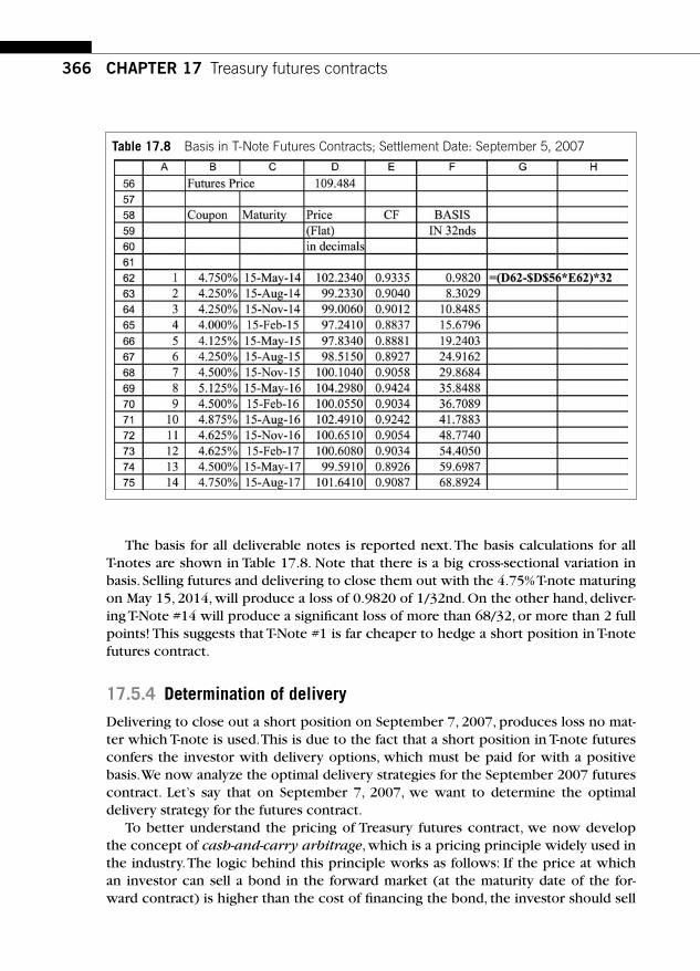
366 CHAPTER 17 Treasury futures contracts
The basis for all deliverable notes is reported next. The basis calculations for all T-notes are shown in Table 17.8 . Note that there is a big cross-sectional variation in basis. Selling futures and delivering to close them out with the 4.75% T-note maturing on May 15, 2014, will produce a loss of 0.9820 of 1/32nd. On the other hand, deliver-ing T-Note #14 will produce a signifi cant loss of more than 68/32, or more than 2 full points! This suggests that T-Note #1 is far cheaper to hedge a short position in T-note futures contract.
17.5.4 Determination of delivery
Delivering to close out a short position on September 7, 2007, produces loss no mat-ter which T-note is used. This is due to the fact that a short position in T-note futures confers the investor with delivery options, which must be paid for with a positive basis. We now analyze the optimal delivery strategies for the September 2007 futures contract. Let’s say that on September 7, 2007, we want to determine the optimal delivery strategy for the futures contract.
To better understand the pricing of Treasury futures contract, we now develop the concept of cash-and-carry arbitrage, which is a pricing principle widely used in the industry. The logic behind this principle works as follows: If the price at which an investor can sell a bond in the forward market (at the maturity date of the for-ward contract) is higher than the cost of fi nancing the bond, the investor should sell
Table 17.8 Basis in T-Note Futures Contracts; Settlement Date: September 5, 2007

367
forward and fi nance the bond. Otherwise, the investor should buy forward and sell the bond in a repurchase transaction. Let’s consider a strategy in which the trader fi nances a deliverable T-bond and sells futures as of September 7, 2007, shown in Figure 17.1 .
Selling futures does not result in cash fl ows. Borrowing and purchasing the note also does not involve any current cash outlay, since the position is fully fi nanced.
Note that the transactions in Figure 17.1 demonstrate how borrowing and buy-ing the underlying deliverable note can hedge a short position in a forward contract. In fact, the hedging strategy is a fully fi nanced position in the underlying note. This implies that a long position in a T-note forward contract is equivalent to borrowing and buying the underlying T-note. Likewise, a short position in the T-bond forward contract is equivalent to shorting the T-note and placing the proceeds in a riskless asset. Note that such transactions will be executed in the repo markets discussed ear-lier in the text. At maturity, the trader can unwind the trade as shown in Figure 17.2 .
At the time the position is unwound, the seller will receive the conversion factor adjusted futures price plus the accrued interest as of maturity date T. This amount is CF � Ht ( s ) � aiT. We denote accrued interest at date T by aiT . The seller must deliver the bond to close out his short position; to accomplish this he must pay back the money borrowed plus interest, which is (in the absence of a coupon payment between dates t and T ):
F P ai rT t
t t t� � ��
( ) .1360
⎛⎝⎜⎜⎜
⎞⎠⎟⎟⎟ (17.1)
The quantity Ft is the forward price of the bond and it is the break-even price; if the trader receives this price on delivery into futures markets, he will break even.
17.5 Treasury futures contracts
Buy bond Pay cash
Receive cash
Post bond ascollateral
Futurestrader
Repodealer
Financing bonds
Trader finances a deliverable T-bond andsells futures now
FIGURE 17.1
Financing Bonds for Delivery
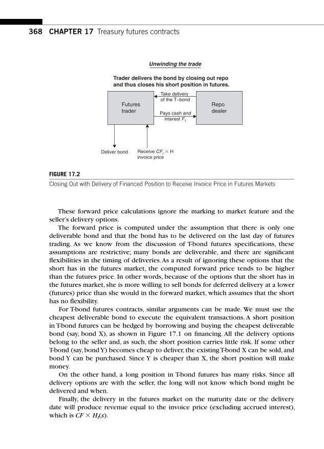
368 CHAPTER 17 Treasury futures contracts
These forward price calculations ignore the marking to market feature and the seller’s delivery options.
The forward price is computed under the assumption that there is only one deliverable bond and that the bond has to be delivered on the last day of futures trading. As we know from the discussion of T-bond futures specifi cations, these assumptions are restrictive; many bonds are deliverable, and there are signifi cant fl exibilities in the timing of deliveries. As a result of ignoring these options that the short has in the futures market, the computed forward price tends to be higher than the futures price. In other words, because of the options that the short has in the futures market, she is more willing to sell bonds for deferred delivery at a lower (futures) price than she would in the forward market, which assumes that the short has no fl exibility.
For T-bond futures contracts, similar arguments can be made. We must use the cheapest deliverable bond to execute the equivalent transactions. A short position in T-bond futures can be hedged by borrowing and buying the cheapest deliverable bond (say, bond X), as shown in Figure 17.1 on fi nancing. All the delivery options belong to the seller and, as such, the short position carries little risk. If some other T-bond (say, bond Y) becomes cheap to deliver, the existing T-bond X can be sold, and bond Y can be purchased. Since Y is cheaper than X, the short position will make money.
On the other hand, a long position in T-bond futures has many risks. Since all delivery options are with the seller, the long will not know which bond might be delivered and when.
Finally, the delivery in the futures market on the maturity date or the delivery date will produce revenue equal to the invoice price (excluding accrued interest), which is CF � Ht ( s ).
Deliver bond Receive CF i � Hinvoice price
Pays cash andinterest F t
Take deliveryof the T–bond
Futurestrader
Repodealer
Unwinding the trade
Trader delivers the bond by closing out repoand thus closes his short position in futures.
FIGURE 17.2
Closing Out with Delivery of Financed Position to Receive Invoice Price in Futures Markets

369
17.5.5 Basis after carry, or net basis
The forward price represents the price at which the bond can be sold forward to break even. The invoice price represents the actual revenue by willing the bond in the futures market. Therefore, the difference between the forward price of the bond and the invoice price measures the profi t or loss associated with the strategy of sell-ing futures and borrowing and buying the bond. This difference is what is known as the basis after carry (BAC), or net basis, and is given by
F CF H st t� � ( ). (17.2)
We show the calculations of forward price and net basis in Table 17.9 . The for-ward price is the cost of carrying a deliverable bond through repo fi nancing until the delivery date of the futures contract. The conversion factor times the futures price is the revenue associated with delivery. The difference between the two (as shown in Equation 17.2) measures the loss or profi t associated with a cash-and-carry position.
The transactions on the delivery date to unwind the positions in futures and bond markets are shown in Figure 17.2 . This concept is widely used by bond traders who study the spread between futures and forward prices. The BAC measures the net cost of carrying the bond in a repurchase transaction and delivering it into the futures market and receiving the invoice price. If the basis and BAC are negative, profi ts are realized by this arbitrage strategy.
Typically, the basis and BAC are positive, as Table 17.9 illustrates. Forward price is calculated in Table 17.9 as per Equation 17.1, and the BAC is calculated as per Equation 17.2.
Note that the basis after carry can be split into two components: the basis and the carry. Intuitively, we can write BAC as follows: BAC � Basis � Reinvested cash
17.5 Treasury futures contracts
Table 17.9 Computation of Forward Price and Net Basis

370 CHAPTER 17 Treasury futures contracts
infl ows � Financing costs. When the carry is positive, the BAC is less than the basis; otherwise, it is greater than the basis.
For Bond #1 in Table 17.10 , the basis stood at one tick, or 1/32nds. The carry was negative, since the fi nancing cost was 4.83% (repo rate) on a market price that was above 100, whereas the accrued interest was 4.75% on the par value of 100. This is the reason that the net basis is higher than the basis.
Traders can minimize their losses by delaying delivery in a positive carry market if there are no adverse price movements. It is worth remembering that when BAC � 0 there will be arbitrage opportunities. This requires selling futures and borrowing and buying the cheapest bond for delivery. The bond transaction will be positioned through a repo desk. On the other hand, if BAC � 0, there is no riskless arbitrage opportunity; if we try to buy futures and short the cheapest bond, there is always the risk that on the delivery month some other bond might become cheaper to deliver. If this were to happen, that bond will be delivered and the short position will have to be covered, perhaps at a considerable cost. Usually the traders use the BAC of a deliverable bond to determine which bond is cheap-est to deliverable issue (CDI) or the cheapest to deliver (CTD). On a daily basis, the BAC is calculated for each deliverable issue, and the issue that has the lowest BAC is identifi ed as the CDI. In the computations of BAC, a fi nancing rate of 4.83% is assumed for all T-bonds.
17.5.6 Implied repo rate
A related concept is the implied repo rate. This concept computes the internal rate of return associated with the strategy of selling T-bond futures, and borrowing and buying an eligible T-bond and delivering it to the futures market at maturity. In the expression that we derived for the basis after carry, we set BAC � 0 and solve for the fi nancing rate r* as the implied repo rate. The resulting expression for the implied repo rate is
rCF H P ai
cai
P aiT t c T s
i it T t
it t
*
( )
.�� � � �
� ��
� ��
×
⎡
⎣⎢⎢
⎤
⎦⎥⎥
2
360 2 360(17.3)
Equation 17.3 is valid when there is a coupon payment at date s prior to the maturity date T of the futures contract. If there is no coupon payment, the equation can be simplifi ed by setting c � 0 in Equation 17.3 to get the implied repo rate as:
rCF H P ai ai
P ai T ti it T t
it t
*( )
.�� � � �
��
�
⎡
⎣⎢⎢
⎤
⎦⎥⎥
360(17.4)
The implied repo rates for all deliverable bonds are shown in Table 17.10 . Note that T-Notes #3 to #14 all have negative implied repo rates. This implies that a short
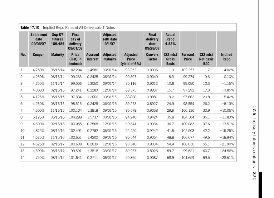
37
11
7.5
Treasury futures contracts
Table 17.10 Implied Repo Rates of All Deliverable T-Notes
Settlement date
09/05/07
Sep-07 futures
109.484
First day of
delivery 09/01/07
Adjusted settl date 9/1/07
Final delivery
date 09/28/07
Actual Repo
4.83%
No. Coupon Maturity Price (Flat) in decimals
Accrued Interest
Adjusted maturity
Adjusted Price
(yield of 6%)
Convers Factor
(32 nds) Gross Basis
Forward Price
(32 nds) Net basis
BAC
Implied Repo
1 4.750% 05/15/14 102.234 1.4586 03/01/14 93.353 0.9335 1.0 102.257 1.7 4.02%
2 4.250% 08/15/14 99.233 0.2425 06/01/14 90.397 0.9040 8.3 99.274 9.6 0.10%
3 4.250% 11/15/14 99.006 1.3050 09/01/14 90.116 0.9012 10.8 99.050 12.3 � 1.15%
4 4.000% 02/15/15 97.241 0.2283 12/01/14 88.375 0.8837 15.7 97.292 17.3 � 3.85%
5 4.125% 05/15/15 97.834 1.2666 03/01/15 88.808 0.8881 19.2 97.882 20.8 � 5.42%
6 4.250% 08/15/15 98.515 0.2425 06/01/15 89.273 0.8927 24.9 98.554 26.2 � 8.13%
7 4.500% 11/15/15 100.104 1.3818 09/01/15 90.579 0.9058 29.9 100.136 30.9 � 10.06%
8 5.125% 05/15/16 104.298 1.5737 03/01/16 94.240 0.9424 35.8 104.304 36.1 � 11.83%
9 4.500% 02/15/16 100.055 0.2568 12/01/15 90.344 0.9034 36.7 100.083 37.6 � 13.51%
10 4.875% 08/15/16 102.491 0.2782 06/01/16 92.420 0.9242 41.8 102.503 42.2 � 15.25%
11 4.625% 11/15/16 100.651 1.4202 09/01/16 90.544 0.9054 48.8 100.677 49.6 � 18.94%
12 4.625% 02/15/17 100.608 0.2639 12/01/16 90.340 0.9034 54.4 100.630 55.1 � 21.90%
13 4.500% 05/15/17 99.591 1.3818 03/01/17 89.257 0.8926 59.7 99.621 60.7 � 24.56%
14 4.750% 08/15/17 101.641 0.2711 06/01/17 90.865 0.9087 68.9 101.659 69.5 � 28.51%

372 CHAPTER 17 Treasury futures contracts
position in futures hedged with any one of these bonds will produce a loss. T-Note #1 has a positive implied repo rate of 4.02%, which is still less than the actual repo rate of 4.83%. The difference between these two rates is the price that one has to pay for being short in T-note futures. This is because a short position in T-note futures con-fers delivery options to the seller, and the market assigns a price for such options.
We can directly apply Equations 17.3 and 17.4 to determine the implied repo rate. The following example illustrates this idea.
Example 17.4 September 2007 T-note futures were quoted at 109.484. The deliverable bond 4.75%, May 15, 2014, was selling at a fl at price of 102.2340 for settlement on September 5, 2007. The
FIGURE 17.3
Determination of Implied Repo Rates
373
conversion factor of this bond was 0.9335. Determine its implied repo rate. If the actual repo rate was 4.83%, was there an arbitrage?
Let’s make some initial calculations: The accrued interest on September 7, 2007 � ait � 1.45856. The accrued interest on September 30, 2007 � aiT � 1.7554. The futures price Ht ( T ) � 109.484. The conversion factor � CF i � 0.9335. The cash price of the bond � Pit � 102.234.
Since there was no coupon between September 5, 2007, and September 30, 2007 (which is the delivery date), we can set c � 0 in Equation 17.3 to solve for the implied repo:
r* . . . . .( . . )
�� � � �
�
0 9335 109 484 102 234 1 7554 1 45856102 234 1 45856
⎡
⎣⎣⎢⎢
⎤
⎦⎥⎥� �
36023
4 02. %.
We can also determine by trial and error the fi nancing rate at which the forward price was exactly equal to the conversion factor times the futures price. This latter approach can be exe-cuted in Excel using the Solver function, as done in Figure 17.3 .
The Solver sets the forward price in cell B157 to be equal to the conversion fac-tors multiplied by the futures price (as in cell J157) by fi nding the correct fi nancing rate in cell A157. This condition ensures that the net basis will be zero.
17.5.7 Duration bias in deliveries
We have shown that for the September 2007 T-note contract, the relatively high-coupon (4.75% coupon) and short maturity T-note had the lowest net basis and highest implied repo rate. This T-note had relatively short duration of all the deliverable issues. In general, is there a duration bias? To address this question, we examine the circum-stances under which low-coupon bonds and notes or high-coupon bonds and notes may be cheaper to deliver. To do this, we vary the yield from 1% to 15% in Figure 17.4 .
We compute the ratio of price to the conversion factor for the high-coupon and the low-coupon bonds and notes.
At yield levels below 6%, we fi nd that the high-coupon bond has a lower ratio. This suggests that at higher yields, low-coupon long-maturity bonds are cheaper to deliver. Conversely, at low yields, high-coupon, short-maturity bonds are cheaper to deliver. The economic reasoning behind this statement is the following: As rates fall, all bonds appreci-ate in price, but low-coupon, long-maturity bonds tend to become relatively more expen-sive; hence it is cheaper to deliver high-coupon, short-maturity bonds. In a similar manner, as the rates go up, all bonds become cheap, but the low-coupon, long-maturity bonds tend to become cheaper than the high-coupon, short-maturity bonds. As a consequence, low-coupon, long-maturity bonds are delivered during periods of high interest rates.
17.5.8 Hedging applications
Treasury bond and note futures contracts are used in fi xed income markets to hedge underlying positions in Treasury bonds, corporate bonds, and mortgage-backed
17.5 Treasury futures contracts

374 CHAPTER 17 Treasury futures contracts
securities. Given the liquidity of Treasury bond and note futures contracts as illustrated inTable 17.6 , this is hardly surprising. An application of bond futures is shown next.
Example 17.5 Consider a dealer who has a long position in a $100 million, par value of 5.125%, May 15, 2016, Treasury note. He would like to hedge his position with the September 2007 T-note futures. The cheapest deliverable bond to this futures contract is a 4.75%, May 15, 2014, Treasury note. How many futures contracts must the dealer sell to hedge his long position in the 5.125%, May 15, 2016, note?
To properly hedge the Treasury note, we must sell n futures contracts such that the following holds:
n PVBP PVBP� �( ) ( ).Futures Note to be hedged
The logic behind the hedge can be broken into the following steps: First, determine the cheap-est deliverable note. This is the one with the lowest BAC or net basis. This information was provided in Table 17.10 . Second, fi nd the DV01 or PVBP of the cheapest deliverable note. Third, recognize that the PVBP of T-note futures is the PVBP of the cheapest note adjusted by its conversion factor; this is due to the fact that the T-note futures tend to track the cheapest deliverable T-note. For this note the BAC is close to zero, ignoring delivery options. Therefore, as a fi nal step, we set the forward price (the break-even price) equal to the conversion factor adjusted futures price. Setting BAC � 0, we get
CF P a rT t
aiit it T� � � � ��
�Futures Price ( ) 1360
⎛⎝⎜⎜⎜
⎞⎠⎟⎟⎟⎟
High duration bonds
Price/CF
Low duration bonds
1
6%Yields
FIGURE 17.4
Duration Bias in Deliveries

375
or
CF PVBP PVBP r� � � �( ) ( )Futures Price Cheapest Deliverable Note 1TT t�
360
⎛⎝⎜⎜⎜
⎞⎠⎟⎟⎟⎟.
Substituting equation into equation, we get the following hedge ratio, n :
nCF PVBP
PVBP rT t
��
��
( )( )
.Note to be hedged
Cheapest Note1
1360
(17.5)
It is easy to verify that the PVBP of the 5.125% T-note is 730, and the PVBP of the cheapest deliverable note is 583. Using this information in Equation 17.5, we can determine the hedge ratio as follows:
n ��
�
�0 9335 730
5831
1 0 048323
360
1 1653.
.. .
Note that the futures contract is on a $100,000 par amount. Therefore, to hedge $100 mil-lion par, we must sell 100 � 10 � 1.1653 � 1165.3, or about 1165 contracts.
SUGGESTED READINGS AND REFERENCES The following papers in academic research dwell in detail on forward contracts, futures contracts,
Treasury futures contracts, and delivery options.
Cox , J. , Ingersoll , J. , & Ross , S. ( 1981 ) . The relation between forward prices and futures prices . Journal of Financial Economics , 9 ( 4) , 321 – 346 .
Garbade , K. D. , & Silber , W. L. ( 1983 ) . Futures contracts on commodities with multiple varieties: An analysis of premiums and discounts . Journal of Business , 56 , 249 – 271 .
Gay , G. D. , & Manaster , S. ( 1984 ) . The quality option implicit in futures contracts . Journal of Financial Economics , 13 , 353 – 370 .
Gay , G. D. , & Manaster , S. ( 1986 ) . Implicit delivery options and optimal delivery strategies for fi nan-cial futures contracts . Journal of Financial Economics , 16 , 41 – 72 .
Jarrow , R. , & Oldfi eld , G. ( 1981 ) . Forward contracts and futures contracts . Journal of Financial Economics , 9 ( 4) , 373 – 382 .
Kilcollin , T. E. ( 1982 ) . Difference systems in fi nancial futures markets . Journal of Finance , 37 , 1183 – 1197 .
Livingston , M. ( 1984 ) . The cheapest deliverable bond for the CBT treasury bond futures contract . Journal of Futures Markets , 4 , 161 – 172 .
Richard , S., & Sundaresan , M. ( 1981 ) . A continuous tune model of forward prices and futures prices in a multigood economy . Journal of Financial Economics , 9 ( 4) , 347 – 371 .
Suggested readings and references

This page intentionally left blank

377Fixed Income Markets and Their DerivativesCopyright 2009 by Academic Press. Inc. All rights of reproduction in any form reserved.
CHAPTER SUMMARY Credit default swaps (CDSs) are contracts that are available in the dealer markets for either assuming or reducing the credit risk exposure associated with one or more obligors (names). This chapter contains an analysis of CDSs and their applications in risk management. It describes CDS contracts and the evolution of documenta-tion concerning admissible credit events covered by the contract. In addition, the evolution of indexes and CDX contracts are described. The valuation principles are outlined, and the need for better back-offi ce systems, marking to market, and clear-inghouse safeguards are stressed.
18.1 CREDIT DEFAULT SWAPS Credit derivatives are typically bilateral contracts that enable one party to either assume or reduce credit exposure on one or more debt obligations of named issuers. Corporations, banks, or sovereign entities may have issued such obligations. It should be emphasized that the issuer is typically not a direct party to the credit derivatives agreement. The notional value of credit derivatives contracts is estimated at about $65 trillion. This is a signifi cant amount considering the fact that the market only began in the mid-1990s.
A single-name credit default swap (CDS) is an over-the-counter (OTC) contract that allows one party to sell insurance on a named debt obligation to another party. Therefore, in a single-name CDS, there are two parties: the buyer of protection and the seller of protection. Consider a single-name CDS with the following terms: The swap has a maturity of fi ve years, and the underlying obligor is IBM. The buyer of
Credit default swaps: Single-name, portfolio, and indexes 18
CHAPTER

378 CHAPTER 18 Credit default swaps: Single-name, portfolio, and indexes
protection agrees to pay (an annualized) premium of 50 basis points every quarter until either the maturity date of the swap or the fi rst time a contractually specifi ed credit (trigger) event occurs, whichever comes fi rst. The 50 basis points may be thought of as an insurance premium. Table 18.1 illustrates the terms of a hypotheti-cal CDS transaction.
The buyer of protection pays a periodic fee called the credit default swap pre-mium. The buyer of protection will benefi t if the value of reference debt obligation goes down. This might happen because the obligation is downgraded by rating agen-cies or if the spreads of reference obligation widen in the market due to worsening credit reputation. The buyer benefi ts whenever the value of the obligation goes down. In this sense, the buyer is said to be short in the reference obligation. If any one of the specifi ed trigger events occurs, the buyer can deliver the reference obligation (or one of the many deliverable obligations specifi ed in the contract) and receive the par value of the amount covered by the contract. Thus the buyer receives the difference between the par value and the market value of the delivered obligation. Typically, the trigger events covered by the swap will include six credit events, which are (a) bank-ruptcy, (b) failure to pay outstanding debt obligations, (c) repudiation or moratorium, (d) obligation acceleration, (e) obligation default, and (f) restructuring of a loan or the bond of the reference entity including the reference obligation. By convention, the buyer is required to pay the accrued CDS premium from the last payment date until the trigger date. The contract is described in Figure 18.1 .
The seller of protection collects the CDS premium every quarter until maturity or the trigger event, whichever comes fi rst. If the trigger event occurs fi rst, the seller will deliver the par value of $10 million and receive from the buyer the defaulted obligations with a par value of $10 million. The buyer is permitted to deliver any of the deliverable reference obligations as specifi ed in the documentation; usually,
Table 18.1 Example of a CDS Contract
Attributes of CDS Specifi cation
Reference Name IBM
Reference obligation Senior note; coupon 6.5%, maturity December 5, 2020
Term of CDS Five years
Notional par value $5 million
Premium 50 basis points (annualized) and payable in quarterly installments
Delivery Options Buyer has the option to deliver specifi ed reference obligations
Trigger events Bankruptcy, liquidation, nonpayment or nontimely payment of promised obligations, etc.
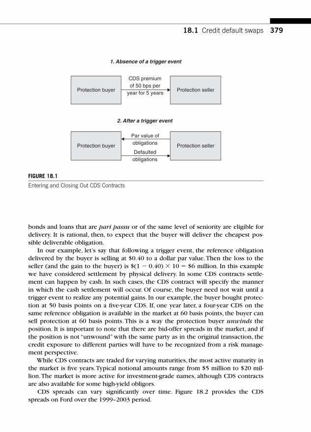
379
bonds and loans that are pari passu or of the same level of seniority are eligible for delivery. It is rational, then, to expect that the buyer will deliver the cheapest pos-sible deliverable obligation.
In our example, let’s say that following a trigger event, the reference obligation delivered by the buyer is selling at $0.40 to a dollar par value. Then the loss to the seller (and the gain to the buyer) is $(1 � 0.40 ) � 10 � $6 million. In this example we have considered settlement by physical delivery. In some CDS contracts settle-ment can happen by cash. In such cases, the CDS contract will specify the manner in which the cash settlement will occur. Of course, the buyer need not wait until a trigger event to realize any potential gains. In our example, the buyer bought protec-tion at 50 basis points on a fi ve-year CDS. If, one year later, a four-year CDS on the same reference obligation is available in the market at 60 basis points, the buyer can sell protection at 60 basis points. This is a way the protection buyer unwinds the position. It is important to note that there are bid-offer spreads in the market, and if the position is not “ unwound ” with the same party as in the original transaction, the credit exposure to different parties will have to be recognized from a risk manage-ment perspective.
While CDS contracts are traded for varying maturities, the most active maturity in the market is fi ve years. Typical notional amounts range from $5 million to $20 mil-lion. The market is more active for investment-grade names, although CDS contracts are also available for some high-yield obligors.
CDS spreads can vary signifi cantly over time. Figure 18.2 provides the CDS spreads on Ford over the 1999 – 2003 period.
Protection buyer Protection seller
Protection buyer Protection seller
1. Absence of a trigger event
2. After a trigger event
CDS premiumof 50 bps per
year for 5 years
Par value ofobligations
Defaultedobligations
FIGURE 18.1
Entering and Closing Out CDS Contracts
18.1 Credit default swaps

380 CHAPTER 18 Credit default swaps: Single-name, portfolio, and indexes
18.2 PLAYERS Who are protection sellers, and who are protection buyers? Table 18.2 gives some idea of who the protection buyers are. Protection sellers are shown in Table 18.3 .
18.3 GROWTH OF CDS MARKET AND EVOLUTION Table 18.4 shows that as of December 2007, CDS contracts reached a notional value of $32 trillion, of which about $17 trillion is accounted for by reporting dealers, about $14 trillion by other fi nancial institutions, and about $7.5 trillion by banks and security fi rms.
FORD 5-year CDS spreads
0
100
200
300
400
500
600
700
10/27/99 11/30/00 01/04/02 02/08/03
2000–2003
Spr
eads
in b
asis
poi
nts
FIGURE 18.2
Example of CDS Spreads, 1999 –2003
Table 18.2 Buyers of Protection, 2006 and 2008
2006 2008
Bank trading desks 39% 36%
Bank loan portfolios 20% 18%
Hedge funds 28% 28%
Corporations 2% 3%
Monoline insurers, insurers, and reinsurers
6% 6%

381
Table 18.3 Sellers of Protection, 2006 and 2008
2006 2008
Bank trading desks 35% 33%
Bank loan portfolios 9% 7%
Hedge funds 32% 31%
Corporations 1% 2%
Monoline insurers, insurers, and reinsurers
17% 18%
Table 18.4 Credit Default Swaps Market, Single-Name Instruments, Notional Amounts Outstanding at End of December 2007 ($ Millions)
Notional AmountsOutstandingBought
Notional AmountsOutstandingSold
Total
All counterparties (net) 24,553,814 24,740,380 32,245,696
Reporting dealers (net) 16,916,296 17,180,706 17,048,500
Other fi nancial institutions 7,283,739 7,245,966 14,529,705
Banks and security fi rms 3,883,281 3,853,134 7,736,415
Insurance and fi nancial guaranty fi rms 165,628 98,504 264,132
Other 3,234,830 3,294,328 6,529,158
Nonfi nancial institutions 353,781 313,709 667,490
MATURITY
Maturity of one year or less 1,589,842 1,511,993 2,002,818
Maturity over one year and up to fi ve years
16,033,096 16,397,447 20,896,394
Maturity over fi ve years 6,930,881 6,830,939 9,346,488
SOVEREIGN/NONSOVEREIGN
Sovereigns 1,409,523 1,390,475 1,797,631
Nonsovereigns 23,144,292 23,349,904 30,448,064
RATING
Investment grade (AAA – BBB) 15,249,114 16,071,251 20,659,294
BB and below 3,751,286 3,715,620 5,010,781
Nonrated 5,553,416 4,953,507 6,575,622
Source: Bank for International Settlements.
18.3 Growth of CDS market and evolution

382 CHAPTER 18 Credit default swaps: Single-name, portfolio, and indexes
CDS contracts within fi ve years of maturity account for a little over $20 trillion, and nonsovereign counterparties account for the vast majority of the amount out-standing. Nearly two thirds of the amount outstanding is of investment grade.
18.4 RESTRUCTURING AND DELIVERABLES The International Swap and Derivatives Association (ISDA) has set forth documen-tation that underlies these contracts. Since the inception of the market, the docu-mentation has evolved infl uencing the types of contingencies that are covered by the CDS contract and the range of reference obligations that the protection buyer may deliver. In part, this is due to the fact that the “restructuring ’’ provision is most diffi cult to incorporate in CDS. First, restructuring is a relatively “soft’’ credit event, and the adverse consequences of such a credit event to the value of reference obli-gations is often not easy to evaluate. Second, restructuring often results in the ref-erence entity retaining a broad set of debt obligations but changing their relative valuation in the market. This may present opportunities to the buyer of protection to strategically exercise their “cheapest deliverable option. ”
Table 18.5 highlights CDS contracts with varying documentation that are avail-able to buyers and sellers.
In 1999, ISDA prescribed the documentation for full restructuring (FR), under which any restructuring was recognized as a trigger event. The buyer was allowed to deliver on a trigger event any reference obligation with a maturity of 30 years. The problems associated with this documentation became clear when, in 2000, the bank debt of Conseco Finance was restructured. This did not necessarily affect the loan investors adversely, since the restructuring included new guarantees and increased coupons. Nevertheless, this was a recognized trigger event under FR documentation,
Table 18.5 Documentation Choices in CDS
Documentation Trigger Events Deliverable Obligations
Full restructuring (FR) Restructurings are included as triggering credit events
Any obligation with less than 30 years to maturity
Modifi ed restructuring (MR) Same as above Deliverable obligations are restricted to those with 30 months (or less) to maturity
Double modifi ed restructuring (MM)
Same as above Deliverable obligations are restricted to those with 60 months (or less) to maturity
No restructuring (NR) Restructurings are excluded from triggering credit events

383
and buyers of protection (typically banks, in this instance) were able to buy long-dated bonds that were trading at a discount and deliver them to the sellers of pro-tection and receive par value in exchange.
To minimize such opportunistic behavior, in 2001 ISDA formulated a modifi ed restructuring (MR) documentation, which retained restructuring as a trigger event but restricted the deliverable obligations to those with a maturity of 30 months or less after the expiration date of a CDS contract. The MR feature thus sharply restricted the menu of deliverable obligations.
In 2003, ISDA issued a further modifi cation to MR, known as MM, under which the remaining maturity of deliverable obligations can be 60 months or less for restructured obligations and 30 months or less for others. This modifi cation refl ected the institutional features in Europe and was also an attempt to increase the choice to the protection buyer, which was sharply restricted under MR.
There are CDS contracts for which restructuring is not recognized as a trigger event. These are known as the NR (for no restructuring) category of CDS contracts. In large part, CDS documentation has evolved to recognize two features of restruc-turing as a trigger event: First, this is a “ soft ” credit event in the sense that the losses associated with restructuring are not easy to estimate. Second, restructuring allows multiple debt claims to remain with signifi cant differences across their values. Since the protection buyer has the option of delivering any of the acceptable reference debt obligations, this “cheapest deliverable option ” becomes rather valuable in restructuring. Figure 18.3 provides a breakdown of CDS contracts across different categories of restructuring. Note that in North America, MR is the dominant docu-mentation used. In Europe MM and FR are more actively used.
Market participants recognize that CDS contracts on the same underlying refer-ence entities with different documentation are different. In fact, the pricing of CDSs
Breakdown of CDS quotes
Total number of quotesby region1
AsiaEuropeNorth AmericaOceaniaOffshore
FR MR MM NR
260,351
53,934118,972
81,5184,490
506
3,86818,931
218,5064,9871,143
248,453
7258,066
24032
104
59,032 58,098
3171,716
55,2200
435
Table 1
1 The numbers do not add up to the total because there are some quotes without regional information.
FIGURE 18.3
Restructuring Clause on CDS Spreads Source: Frank Packer and Haibin Zhu, “ Contractual Terms and CDS Pricing, ” BIS Quarterly Review , 2005.
18.4 Restructuring and deliverables

384 CHAPTER 18 Credit default swaps: Single-name, portfolio, and indexes
with different documentation refl ect the differences in the level of protection from credit events and the loss that can occur conditional on a credit event.
Figure 18.4 shows the CDS spread differences that are attributable to different documentation pertaining to the treatment of restructuring. Note that FR has the highest CDS spread and NR has the lowest CDS spread.
18.5 SETTLEMENT ON CREDIT EVENTS ISDA sets forth rules for settling CDS contracts on the occurrence of credit events. Generally, individual (single-name) CDS contracts are settled by physical delivery. This means that the protection buyer will deliver the defaulted deliverable obligations to the protection seller. In turn, the protection seller will pay par value to the protec-tion buyer. Though this sounds simple in theory, it can become complicated in real life: For one thing, the CDS volume tends to be a multiple of the underlying deliverable obligations. Second, if the deliverable obligations are under Chapter 11 process, there might not be a very liquid market for such obligations. To deal with these issues, ISDA typically will have a protocol associated with settlement of CDS contracts. Cash settle-ment could also be effected in some cases. Typically, this happens when the underly-ing name is part of the index. This requires an auction process.
This auction process requires the auction participants to submit bids and offer prices in an amount of $10 million each. Such submitted bids and offers form the basis for determining what is known as the inside market midpoint. Auction
CDS spread differences
FR–MR FR–NRMM–MR MR–NR
98,833 14,511 34,431 52,232
2.77*3.36*
3.06*1.70*
1.22*0.65*
1.33*1.42*
7.49*7.65*
7.52*4.58*
4.25*4.68*
4.33*2.60*
Number of observationsMean1
Median2
Percentage difference %level (basis points)
Percentage difference %level (basis points)
λ3
1 * shows that the mean is different from zero at a significance level of 95% based on the t-test. 2 * shows that the median is different from zero at a significance level of 95% based on the sign rank test.3 * defined as the ratio between the percentage change in expected losses-given-default and the percentage change in CDS spreads.
1.00 1.35 0.38 �0.30
FIGURE 18.4
Impact of Restructuring Clause on CDS Spreads Source: Frank Packer and Haibin Zhu, “Contractual Terms and CDS Pricing, ” BIS Quarterly Review , 2005.

385
participants also submit limit orders and “ noncompetitive ” market orders. Each bid-ding participant also indicates the aggregate quantity of deliverable obligations that it would need to trade to settle all transactions. This makes the bids more credible from the standpoint of determining the recovery values.
The inside market midpoint is adjusted based on the information from limit orders and market orders as follows: The imbalance of market orders is balanced against the submitted limit orders. For example, in general, the point at which the last limit order is matched becomes the fi nal price. In the auction for Dana Corporation in 2005, dealers submitted bid/offer prices as well as market and limit orders. The inside mar-ket midpoint determined from the submitted bids/offers was 75.125. The totals of market order bids and offers were $56 million and $97 million, respectively, with an imbalance of $41 million of net market “ offers ” (i.e., sell orders). This was balanced against the limit buy orders, from the highest price fi rst. There were fi ve limit bid orders placed between 75.500 and 75.000, each for $10 million. So, the fi fth order at 75.000 was partially fi lled to match $41 million of market imbalance, resulting in the fi nal price of 75.000. 1
We illustrate the issues involved in CDS settlement upon the occurrence of a credit event with a detailed discussion of the Lehman CDS settlement procedure.
Lehman Brothers fi led for bankruptcy on September 15, 2008, an act that rep-resented one of the largest bankruptcy fi lings in the United States and certainly a very large settlement problem in the single-name CDS contracts that were traded on Lehman Brothers. Estimates of Lehman’s debt ranged around $650 billion, and esti-mates of the notional amount of CDS on Lehman were placed around $400 billion. The CDS settlement for Lehman proceeded as follows: October 10 was the auction date. October 15 was the deadline for receipt of Notice of Physical Settlement for trades formed under the Protocol. The settlement date for trades formed under the Protocol was October 20. The fi nal cash settlement date for covered transactions was October 21.
The auction procedure required dealers to submit market orders, limit orders, and requests for physical delivery. The dealers’ bids and offers were reported by ISDA and are reproduced in Table 18.6 . Note that the midpoint resulted in a recovery value of 9.75 cents on $1 notional par value. A total of $4.92 billion par values were requested for physical deliveries.
In addition, limit orders were submitted, and the fi nal adjusted price was set at 8.625.
At a fi rst blush it might appear that with a $400 billion par value and a recovery value of only 8.625 cents on $1 of par value, the settlement could result in a wealth transfer of more than $360 billion from the sellers to buyers. This calculation ignores the fact that many counterparties who sold protection at some point might have bought protection at other points, and vice versa. In addition, parties might have
1See the ISDA protocol and “CDS Recovery Basis: Issues with Index Auctions and Credit Event Valuations,” Nomura Fixed Income Research, April 12, 2006.
18.5 Settlement on credit events

386 CHAPTER 18 Credit default swaps: Single-name, portfolio, and indexes
posted collateral to cover their losses even prior to ISDA settlement. It turns out that in the Lehman CDS settlement, as of October 21 (which was the cash settlement deadline), a total of $6 billion to $8 billion changed hands by close of business. This is approximately 1 –2% of the $400 billion in CDS trades referencing Lehman. The situation might have been more problematic had a few counterparties owing signifi -cant sums on CDS also fi led for bankruptcy at the some time.
18.6 VALUATION OF CDS We begin our valuation of CDS by outlining some important market conventions. First, the premium paid by the protection buyer to the seller is referred to as the
Table 18.6 Settlement of CDS on a Credit Event: The Case of Lehman Brothers Dealer Inside Markets
Dealer Bid Offer Dealer
Banc of America Securities LLC
9.5 11.5 Banc of America Securities LLC
Barclays Bank PLC 8 10 Barclays Bank PLC
BNP Paribas 9 11 BNP Paribas
Citigroup Global Markets Inc.
9.25 11 Citigroup Global Markets Inc.
Credit Suisse Securities (USA) LLC
8 10 Credit Suisse Securities (USA) LLC
Deutsche Bank AG 8 10 Deutsche Bank AG
Dresdner Bank AG 9.5 11.5 Dresdner Bank AG
Goldman Sachs & Co 8.875 10.875 Goldman Sachs & Co
HSBC Bank USA, National Association
10 12 HSBC Bank USA, National Association
JPMorgan Chase Bank, National Association
9 11 JPMorgan Chase Bank, National Association
Merrill Lynch, Pierce, Fenner & Smith Inc.
8 10 Merrill Lynch, Pierce, Fenner &Smith Inc.
Morgan Stanley & Co. Inc. 8.25 10.25 Morgan Stanley & Co. Inc.
The Royal Bank of Scotland PLC
9.25 11.25 The Royal Bank of Scotland PLC
UBS Securities LLC 8.75 10.75 UBS Securities LLC
Note: Inside market midpoint: 9.75.

387
CDS spread, which is typically quoted in basis points per annum of the contract’s notional amount. The payments are made in quarterly installments by the protection buyer to the protection seller. For example, a fi ve-year CDS spread of 400 basis points on Ford debt means that the default insurance on a notional amount of $1 million will cost $40,000 per annum but will be paid in quarterly installments of $10,000.
To motivate the link between CDS spreads and the yield spreads between the underlying bonds over benchmark Treasury, let’s briefl y consider the following port-folio strategy outlined in Table 18.7 . For simplicity, we assume that CDS premiums are paid at the end of each year instead of in quarterly installments. Let’s assume that the CDS premium is $ x and that the IBM debt (deliverable to the CDS) has a dol-lar coupon of $ y. We assume that the IBM bond was bought at a par value of $100. To further simplify analysis, we assume that credit events occur only at year-ends, although the basic economic intuition survives this assumption. The CDS contract has a life of three years.
Note that in Table 18.7 , the payoffs are essentially the IBM coupon less the CDS premium each year. At the end of Year 3, the IBM bond pays $100 par. What happens when there is a credit event, say, at year t � 2 (see Table 18.8 )?
The protection buyer (who is also the bond investor) simply delivers the defaulted bond and receives 100 from the protection seller. Table 18.7 assumes that the IBM bond has paid all the coupons until the default date. Essentially, the bond investor has received promised cash fl ows of $ y each year and the par value
Table 18.7 Payoffs When There Is No Credit Event
Transaction at Date t � 0
Cash Flows at Date t � 0
t � 1 t � 2 t � 3
Buy IBM bond �100 y y y � 100
Buy three-year CDS protection on IBM
0 �x �x � x
Total �100 y � x y � x y � x � 100
Table 18.8 Payoffs When There Is a Credit Event in Year t � 2
Transaction at Date t � 0
Cash Flows at Date t � 0
t � 1 t � 2
Buy IBM bond �100 y y
Buy three-year CDS protection on IBM
0 �x � x � 100
Total �100 y � x y � x � 100
18.6 Valuation of CDS

388 CHAPTER 18 Credit default swaps: Single-name, portfolio, and indexes
until Year 2. In effect, this is similar to owning a risk-free bond until the credit event occurs. The buyer of CDS protection still has no control over when the default may occur, but he will receive the par value when it occurs. This suggests that the dif-ference between the bond yield and the CDS premium (expressed in percentage) should be closely linked to the risk-free rate. In other words, we may expect the following:
Bond yield CDS premium Risk-free rate.� �
But the risk-free rate that we can infer by computing the spread between the bond yield and the CDS premium might not conform to the properties of proxies of risk-free rate (such as T-bill yields or repo rates) because of the uncertainty about the timing of default.
18.6.1 CDS spreads, probability of default, and recovery rates
CDS spreads have a tight link to the probability of default of the underlying deliver-able obligations and the recovery rates that the debt investors may get conditional on a credit event. We illustrate this link with a very simple example in which we consider a one-year CDS contract. We make the simplifying assumption that the CDS premium ( x) is paid up front instead of in quarterly installments. We also ignore dis-counting to keep matters simple. Let’s denote by p the default probability and by R the recovery rate. Note that in Figure 18.5 , with a probability p, there is a credit event and the bond is worth only R. Then the protection buyer can deliver the bond and get $1. Hence his payoffs are 1 � R. With a probability of 1 � p, there is no credit event during the life of the CDS.
The expected payoff to the protection buyer is then (1 � R)p. The protection buyer and the seller will enter into a CDS transaction only if the CDS premium, x, is set such that the value of the swap transaction is zero. This leads to the condition that x � (1 � R)p.
In this simple illustration, the CDS premium is simply the product of default prob-ability and the loss (1 � R) associated with default. If we make the assumption that the recovery rates are known, we can back out the default probability from observed
1-R
p
Pay $x
1-p0
FIGURE 18.5
Pricing CDS Spreads

389
CDS premiums. For example, with a recovery rate of 50% and a CDS premium of 400 basis points (4%), we have the following equality:
4 1 0 5% ( . )� � p
implying that the default probability, p , is 8%. Let’s now generalize these ideas to a multiple-period setting to derive the value
of the CDS premium on a CDS contract with a life of fi ve years. Let the premiums be paid in quarterly installments. We assume that there is a zero coupon curve for each maturity of interest. The following notation will be used: zero coupon price at time 0 for payment of $1 at time i � 0 is z (0, i ).
The survival probability (for the underlying debt issuer) at date i is denoted by q(i). Note that the survival probability is 1 minus the probability of default. We make the simplifying assumption that the protection buyer and seller will not default on their obligations. The sum of the discounted value of all payments made by the pro-tection buyer can be then specifi ed as follows:
z i q ix
i
( , ) ( )041
20
�∑ (18.1)
Equation 18.1 simply takes each quarterly scheduled payment and multiplies it by the survival probabilities, then discounts them back to date 0. It then totals them all. Typically, the protection buyer is also responsible for paying the accrued inter-est from the last installment date to the date on which a credit event occurs. Assuming that the credit event always occurs exactly at the middle of two installment dates enables us to derive a simple formula. First, we need to compute the probability that the issuer survives until date i � 1 but not until date i. This is simply q(i � 1) � q(i). Then the accrued interest payable for a credit event occurring in this interval is
[ ( ) ( )] .q i q ix
� �14
1
2
We can add across all the installment dates the discounted accrued interest to get
z i q i q ix
i
( , )[ ( ) ( )] .0 14
1
21
20
� ��∑ (18.2)
Adding Equations 18.1 and 18.2 we get the present value of all cash fl ows that the protection buyer should pay the protection seller:
z i q ix
z i q i q ix
i i
( , ) ( ) ( , )[ ( ) ( )] .04
0 14
1
21
20
1
20
� �
� � �∑ ∑ (18.3)
The protection seller will have to make a contingent payment if a credit event occurs. The present value of the payments that the seller must make can be specifi ed as follows: The probability of a credit event occurring between dates i � 1
18.6 Valuation of CDS

390 CHAPTER 18 Credit default swaps: Single-name, portfolio, and indexes
and i is q ( i � 1) � q(i). The obligation of the protection seller is (1 � R). The dis-counted value of this is simply z(0, i )(1 � R)[q ( i � 1) � q ( i)]. We sum across all pos-sible installment dates to get the present value of contingent payments to be made by the protection seller, as shown here:
( ) [ ( ) ( )] ( , )1 1 01
20
� � ��
R q i q i z ii∑ (18.4)
Setting the present value of the payments of the protection buyer (as given by Equation 18.3) to the present value of payments to be made by the protection seller (as given by Equation 18.4), and solving for the CDS premium, we get
x
R z i q i q i
z i q i z
i
i
�
� � �
�
�
�
( ) ( , )[ ( ) ( )]
( , ) ( ) ( ,
1 0 1
01
40
1
20
1
20
∑
∑ ii q i q ii
)[ ( ) ( )]� ��
11
81
20
∑(18.5)
We illustrate the basic idea outlined previously with a simple example of pricing a two-year CDS. In this example, which is presented in Figure 18.6 , we take the zero curve (shown in Column G) and the survival probabilities (shown in Column H) as inputs to our model. They are shaded. We determine the CDS premium by trial and error (using the Excel Solver function) such that the present value of the payments made by the protection buyer is exactly equal to the present value of the payments made by the protection seller. The worksheet is constructed as follows:
■ Column I provides the quarterly payments made by the protection buyer. We initially guess a number but eventually use the Solver function to determine the correct CDS premium.
■ Column J is the expected CDS payments in each quarter. This is obtained by multiplying the CDS premium in Column I by the survival probability in Column H. At this stage, the numbers are reported in basis points.
■ Column K computes the present value of payments made by the protection buyer on the notional principal of $1 million. This is obtained by multiplying the entry in Column J (which contains the expected CDS payments) by the corresponding discount factor in Column G. We multiply the resulting amount by $1 million and divide by 10,000 to refl ect the fact that CDS premium is in basis points (which is 1/100th of 1%).
■ Column L computes the probability of default as 1 minus the survival prob-ability (which is in Column G). The probability of default in Cell L16 is the dif-ference between the survival probability in Cell G15 and the one in Cell G16.
■ The expected accrual payments are presented in Column M by multiplying the default probability in Column L with one half the quarterly CDS premium.

391
■ Column N computes the present value of accrual payments on the notional principal.
■ Column O computes the present value of contingent payments to be made by the protection seller on the notional principal.
The worksheet shown in Figure 18.6 illustrates a two-year CDS valuation. Normally we begin with a guess for CDS premium and change it until the present value of the cash fl ows to be paid by the protection buyer is exactly equal to the present value of contingent payments to be made by the protection seller. We can use the Excel Solver function to compute the correct CDS premium as shown in Figure 18.7 .
Note that Solver is choosing the CDS premium in Cell I3 such that the present value of the protection payments exactly matches the present value of payments to be made by the protection seller. For this two-year CDS, the correct premium turns out to be 37.818 basis points per quarter.
18.6.2 Applications
CDS contracts can be used to manage the risk-return properties of credit risky secu-rities such as bonds and loans. For example, consider the strategy of buying $10 mil-lion par value of the reference obligation with a coupon of 8% and simultaneously buying protection with a fi ve-year single-name CDS. In this strategy, the investor will receive an 8% coupon when there is no trigger event and is guaranteed to receive
FIGURE 18.6
CDS Valuation
18.6 Valuation of CDS
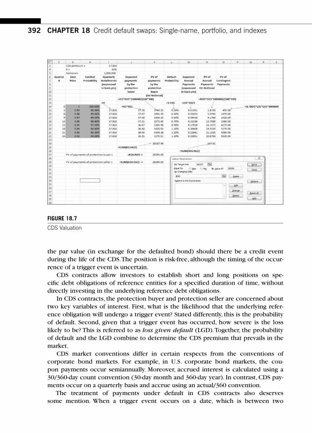
392 CHAPTER 18 Credit default swaps: Single-name, portfolio, and indexes
the par value (in exchange for the defaulted bond) should there be a credit event during the life of the CDS. The position is risk-free, although the timing of the occur-rence of a trigger event is uncertain.
CDS contracts allow investors to establish short and long positions on spe-cifi c debt obligations of reference entities for a specifi ed duration of time, without directly investing in the underlying reference debt obligations.
In CDS contracts, the protection buyer and protection seller are concerned about two key variables of interest. First, what is the likelihood that the underlying refer-ence obligation will undergo a trigger event? Stated differently, this is the probability of default. Second, given that a trigger event has occurred, how severe is the loss likely to be? This is referred to as loss given default (LGD). Together, the probability of default and the LGD combine to determine the CDS premium that prevails in the market.
CDS market conventions differ in certain respects from the conventions of corporate bond markets. For example, in U.S. corporate bond markets, the cou-pon payments occur semiannually. Moreover, accrued interest is calculated using a 30/360-day count convention (30-day month and 360-day year). In contrast, CDS pay-ments occur on a quarterly basis and accrue using an actual/360 convention.
The treatment of payments under default in CDS contracts also deserves some mention. When a trigger event occurs on a date, which is between two
FIGURE 18.7
CDS Valuation

393
coupon dates, the seller of protection is contractually entitled to receive an accrued coupon payment until the date of default. In the case of a corporate bond, the unpaid accrued interest will remain a claim on borrower’s assets and will be resolved through the fi nancial distress resolution process (such as workouts, Chapter 11, etc.).
18.7 CREDIT-LINKED NOTES Credit-linked notes (CLNs) are very similar to CDS except that the buyer has a col-lateral at the time the transaction is initiated. The protection buyer sells CLNs by promising a coupon rate and a stated maturity. If a credit trigger specifi ed in the CLN occurs, all the promised payments are suspended. The protection buyer simply delivers the defaulted debt or loan obligations. Figure 18.8 illustrates the way CLN contracts are entered into and how they are closed out.
Special-purpose vehicles typically issue CLNs, and they trade like corporate bonds. The protection buyer sells the CLN and commits to make periodic payments until the reference entity undergoes a “trigger event. ” The buyer of CLNs is in fact the pro-tection seller, and she pays for the CLN at the time the CLN is sold and can hope to collect the principal back only if “trigger events ” do not occur for the reference entity during the life of CLN. If and when the “trigger event ” occurs, the seller of the CLN will deliver the defaulted debt securities and keep the cash that was paid by the buyers of the CLN at the time of sale.
Protection buyer Protection seller
Protection buyerissues CLN
Protection sellerbuys CLN
1. Absence of a trigger event
2. After a trigger event
Delivers defaultedobligations of ref.entity.
Pays couponof 8% and thepar at maturity
Receives proceedsat the time of issue
FIGURE 18.8
Entering Into and Closing Out CLN Contracts
18.7 Credit-linked notes
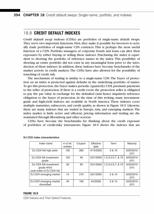
394 CHAPTER 18 Credit default swaps: Single-name, portfolio, and indexes
18.8 CREDIT DEFAULT INDEXES Credit default swap indexes (CDXs) are portfolios of single-name default swaps. They serve two important functions. First, they make it possible for investors to actu-ally trade portfolios of single-name CDS contracts. This is perhaps the most useful function of a CDX. Portfolio managers of corporate bonds and loans can alter their exposures by either buying or selling these indexes. Purchasing the index is equiv-alent to shorting the portfolio of reference names in the index. This possibility of shorting an entire portfolio did not exist in any meaningful form prior to the intro-duction of these indexes. In addition, these indexes have become benchmarks of the market activity in credit markets. The CDXs have also allowed for the possibility of tranching of credit risk.
The mechanism of trading is similar to a single-name CDS. The buyer of protec-tion on an index is protected against defaults in the underlying portfolio of names. To get this protection, the buyer makes periodic (quarterly) CDX premium payments to the seller of protection. If there is a credit event, the protection seller is obligated to pay the par value in exchange for the defaulted (and hence impaired) reference obligation to the buyer of protection. At the time of this writing, many investment-grade and high-yield indexes are available in North America. These indexes cover multiple maturities, subsectors, and credit quality, as shown in Figure 18.9 . Likewise, there are many indexes that are traded in Europe, Asia, and emerging markets. The index market is fairly active and effi cient; pricing information and trading are dis-seminated through Bloomberg and other screens.
CDXs have become the benchmarks for thinking about the credit exposure of portfolios of credit-risky instruments. Figure 18.9 shows the indexes that are
DJ CDX index characteristics
Index name # of ref.entities
Coupon Effectivedate
Term Maturity
6/20/2010(5Y)
5 & 104/14/2005360100DJ CDX NA high yield
6/20/2010(5Y)
1,2,3,4,5,7, & 103/21/200540125DJ CDX NA investmentgrade
6/20/2010(5Y)
5 & 103/21/200521014DJ CDX emerging market
5 & 104/4/200516040 6/20/2010(5Y)
DJ CDX emerging marketdiversified
6/20/2010(5Y)
1,2,3,4,5,7, & 103/21/20059030DJ CDX NA investmentgrade HiVol
(sub-index of DJ CDX IG)
FIGURE 18.9
CDX Indexes and Their Salient Features

395
currently available for trading. The indexes are constructed by Dow Jones and maintained by Markit partners. There are 16 North American credit derivative trad-ing desks with which Markit works in managing the credit derivative indexes. This requires many activities, including the following:
1. Conduct all dealer polls regarding the selection of the underlying credits. 2. Select underlying reference obligations following the selection of the refer-
ence entities. 3. Collect daily end-of-day prices from more than 15 institutions. 4. Calculate and publish composite price and spread as well as theoretical price
and spread on www.markit.com . 5. Release the offi cial composite price and spread to Dow Jones for publication
in The Wall Street Journal.
For example, the Dow Jones High Yield Index of North America (referred to as the DJ CDX North America High Yield Index) is composed of a static portfolio of 100 equally weighted high-yield CDS entities domiciled in North America. We outline the key features of CDX indexes next.
The indexes are characterized by many important design features. First, the under-lying portfolio is static; this implies that once the CDX is computed, no names can be added or deleted from the portfolio. These static portfolios are equally weighted. The newly constructed (minted) CDX is referred to as the on-the-run index. However, as time passes, the index becomes less relevant, and new indexes are introduced periodically. This second feature is very similar to the on-the-run and off-the-run benchmarks in the Treasury markets. Third, the CDX market operates on established payment and maturity dates to ensure standardization: the 20th of March, June, September, and December of every year. These dates also constitute maturity dates where applicable.
Another important feature of CDX is the fact that spread on the CDX is deter-mined at the time it is put together; this is referred to as the deal spread, which is paid on a quarterly basis. This implies that as the market conditions change, some up-front payment might be needed to refl ect the difference between the deal spread and the current spread.
Protection buyers who enter into a CDX index transaction between two payment dates will be compensated for the amount of accrued premium by the protection seller. This is done to refl ect the fact that the protection buyer would pay the CDX premium for the full quarter on the following payment date. The buyer of protection gets protection only from the time he bought protection, which is in effect only for part of the quarter starting from the day the buyer bought CDX protection.
Earlier in the chapter, we discussed various defi nitions of restructuring. Trading in CDX requires a deeper understanding of the conventions used. Single-name CDS contracts that are the underlying assets for CDX tend to trade with a modifi ed restructuring (MR) provision. But the CDX index tends to trade on an NR basis. In Europe, CDXs tend to use the MM provision.
18.8 Credit default indexes

396 CHAPTER 18 Credit default swaps: Single-name, portfolio, and indexes
SUGGESTED READINGS AND REFERENCES Beck, R. The CDS market: A primer . Risk Analysis Group, Deutsche Bank.
CDS recovery basis: Issues with index auctions and credit event valuations. Nomura Fixed Income Research, April 12, 2006.
ISDA Website on CDS Protocols. http://www.isda.org/
Packer , F. , & Zhu , H. ( 2005, March) . Contractual terms and CDS pricing . BIS Quarterly Review , 1 ,89–100 .
397
CHAPTER
CHAPTER SUMMARY Collateralized debt obligations (CDOs) in which the underlying collateral can be portfolios of loans, corporate bonds, asset-backed securities, mortgage pools, and so on are traded. On the economic strengths of the underlying pools, various bonds are issued with different subordination and seniority in terms of their exposure to default risk and the recovery risk of the underlying pool of collateral. Such bonds are referred to as equity, mezzanine, senior, and super-senior tranches. This chapter describes how CDOs are created and outlines their valuation procedure. The role of the CDX market and its impact on tranched trading of credit risk are discussed.
Structured credit products are created by taking simple credit instruments such as bank loans and corporate bonds as underlying collateral in a special-purpose vehi-cle and then creating different bond-like instruments (known as tranches) for which the cash fl ows depend on the cash fl ows of the underlying collateral. The tranches differ in terms of their exposure to default risk, recovery risk, and the like, depend-ing on the manner in which the structured products are created. We discuss them in detail later in the chapter.
One useful distinction that arises is based on the nature of the underlying col-lateral. If the underlying collateral is made up of assets such as bonds and loans, they are cash assets, and the resulting structured product is directly linked to the properties of the cash assets, which form the collateral. Such structured products are referred to as cash CDOs. Structured products in which the underlying collateral itself consists of credit default swaps are synthetic in the sense that there is an addi-tional layer between the underlying collateral and the assets that serve as the basis for the credit default swaps. Such products are referred to as synthetic CDOs.
Structured credit products: Collateralized debt obligations 19
Fixed Income Markets and Their DerivativesCopyright 2009 by Academic Press. Inc. All rights of reproduction in any form reserved.

398 CHAPTER 19 Structured credit products
19.1 COLLATERALIZED DEBT OBLIGATIONS Collateralized debt obligations (CDOs) are backed by assets held in a special-purpose vehicle (SPV) and managed by an investment manager (the collateral manager). The assets are funded through the issuances of several classes of debt securities, the repayment of which is linked to the performance of the underlying assets that serve as collateral for CDO securities.
Securities issued in a CDO are tranched into two categories:
■ The fi rst category contains rated securities (also known as senior and mezza-nine notes).
■ The second category contains unrated ( “junk” or subordinated notes).
The relative rating is a function of (1) the level of subordination, (2) the extent of overcollateralization, and (3) the priority of payments of interest and principal payments from the underlying collateral. We illustrate the CDO with an example in Figure 19.1 .
Note that the CDO has the underlying collateral as its assets, and the liabilities consist of three tranches of debt issued to fund the purchase of assets. The equity tranche is the fi rst to be exposed to default risk in the underlying pool of assets. If the pool experiences no defaults at all, the equity tranche will receive the stated cou-pon for the term of the contract. On the other hand, if the pool experiences greater than anticipated defaults and greater losses associated with defaults, the equity tranche will absorb all such losses fi rst. As a result, investors in equity tranches will typically demand a higher compensation by way of high coupon rates. The mezza-nine tranche investors are protected by equity investors against default and recovery
Pool of bank loans, orcorporate bonds, or asset-backed securities, ormortgages. The assets mayjust be pools of CDS as well.They may be either purchasedfrom secondary markets ortransferred from the balancesheet of a bank.
AssetsUS $500 million
LiabilitiesUS $500 million
Senior Tranche - $350 million.
Mezzanine Tranche - $100million.
Equity - $50 million.
Example of a Collateralized Debt Obligation (CDO)
FIGURE 19.1
CDO Balance Sheet

399
risks; this will cause them to accept a lower coupon rate than equity holders. Finally, senior tranche investors are protected by both equity and mezzanine investors, and hence they will accept a much lower coupon rate. In addition to default risk and recovery, risk investors in CDOs will face the risk that there is a high correlation of defaults of securities in the underlying pool; this is the correlation risk that investors in CDOs must estimate to correctly determine the appropriate compensation.
19.1.1 CDO structure and players
Figure 19.2 illustrates a simple CDO structure in which we assume that the collat-eral consists of cash assets such as loans and bonds. The SPV issues three classes of securities: senior notes, mezzanine or junior notes, and subordinated securities such as equity. The senior and junior notes constitute the debt associated with the CDO transaction. The proceeds associated with selling these securities will be used to fund the collateral pool of assets.
Cash fl ows generated by the collateral underlying the CDO are used to meet contractual obligations according to a well-defi ned set of rules: First, available cash fl ows are used to pay the collateral manager and trustees of the CDO. Next, princi-pal and interest payments to the note holders are made according to strict senior-ity; senior notes are paid fi rst, and then if cash fl ows are available, the junior notes are paid. Equity holders represent the residual interest in the transaction and receive their payments out of the residual interest proceeds generated by the underlying collateral.
An important aspect of the CDO structure is the treatment of cash fl ows when defaults and default-related losses occur. When the collateral pool experiences
Underlyingcollateral
Special PurposeVehicle [SPV]
Interest ratehedging
arrangements
Trustee
Collateralmanager
Subordinatedsecurities (equity)
Mezzaninefixed/floating
rate notes
Seniorfixed/floating
rate notes
FIGURE 19.2
CDO Structure
19.1 Collateralized debt obligations

400 CHAPTER 19 Structured credit products
defaults, the losses are typically used to write down the par value of equity when there are no residual cash fl ows to equity investors. When default-related losses reach a threshold level, equity can be wiped out, and then write-downs will occur to the par value of the mezzanine tranche, and so on. In this sense, there is a compelling parallel between the CDO liability structure and the liability structure of a fi rm.
There are important differences, however. Unlike a fi rm, which can dynamically change its capital structure, a CDO structure has much less fl exibility in changing its liability structure once it is set up. In addition, the fi rm may be in a much better position to change its assets, issue additional equity, and so on. Equity holders of a CDO structure have technically issued debt (senior and mezzanine) and invested the proceeds in the collateral pool. Thus they have a leveraged stake in the collateral pool. Since losses will be fi rst used to retire equity, equity holders have the high-est risk exposure and will therefore expect higher return. Depending on the extent to which assets in the collateral pool have fi xed or fl oating coupons and how the liabilities are structured (fl oating or fi xed), there could be a mismatch that could introduce an interest rate risk. This is usually dealt with by engaging in interest rate hedging through a swap transaction when the CDO deal is put in place. To further protect debt issued by the SPV, it might be necessary to buy insurance with a mono-cline bond insurance company (such as AMBAC or AIG) and thus provide credit enhancement. The tranches that are so insured are said to have been wrapped, and often they may command higher ratings by rating agencies. The collateral manager is responsible for buying assets and managing them as per the guidelines specifi ed.
The trustee acts as the custodian and performs several key functions: First, the trustee bears responsibility for the safe custody of the assets and for compliance with the guidelines set forth in the CDO structure. Second, the trustee is also respon-sible for computing the contractual payments due to the various players in the CDO transaction. Third, the trustee is responsible for keeping the investors informed about the integrity of the CDO.
19.1.2 Types of cash CDOs
Cash CDOs typically fall into two categories: balance sheet CDOs and arbitrage CDOs. Balance sheet CDO transactions are motivated with a view to obtain regulatory
and/or economic capital relief. In such transactions, a bank might want to take a loan portfolio out of its balance sheet and set up a CDO through the establishment of an SPV, which will fund the purchase of loans by issuing various tranches, as discussed earlier. It should be stressed that the bank will typically retain the equity tranche; this is to ensure that the bank still has the incentive to perform “due diligence ” and make sure that the loans are monitored effectively. By shedding assets through CDOs, the bank is able to reduce the capital requirements. Such transactions are also referred to as collateralized loan obligations, or CLOs.
In contrast, arbitrage CDO transactions attempt to exploit the possibility of sell-ing CDO liabilities (senior debt, mezzanine debt, and equity) at a higher price to fund the underlying collateral pool and have some surplus left over.

401
Cash CDOs can further be classifi ed into two categories: cash-fl ow CDOs and market value CDOs. In cash-fl ow CDOs, the cash fl ows generated by the underlying collateral pool are suffi cient to pay the promised coupon and principal obligations of CDO debt tranches. When there are default-related losses and credit impairments, the CDO structure may dictate that senior tranches are amortized at the expense of junior tranches.
Market value CDOs allow the fund manager to trade the underlying collateral more so as to maintain the market value of the collateral at a level which is more than suffi cient to pay the promised obligations of CDO debt tranches. One of the provisions in a market value CDO is that the collateral pool should be ‘marked to market periodically. ’ This can be a daunting task when the underlying collateral pool consists of assets that are illiquid and that trade (if at all) at a wide bid-offer spread. When the value of the collateral pool falls below a certain threshold level, which is related to the amount of outstanding CDO tranches, assets might have to be liqui-dated to ensure the solvency of the CDO structure. In 1998 CDOs were practically evenly divided between balance sheet CDOs and arbitrage CDOs. But as of 2006, more than 90% of CDOs were of the arbitrage variety.
19.1.3 Synthetic CDOs
Synthetic CDOs are created using credit default swaps (CDSs) as their underlying pool of assets. To create a synthetic CDO, an SPV is set up with the objective of establishing credit risk exposure using CDSs. The main economic objective is to sell tranches of debt securities whereby the debt investors end up selling insurance. In return they receive the premium income generated by the underlying CDS contracts. In economic terms, the buyers of tranches of debt from the SPV are “ long ” in credit risk for which they receive premium income. When the CDS portfolio (the underly-ing collateral pool) experiences default risks and losses associated with default, such losses are “passed through ” in strict order of priority: Equity tranches bear the losses at the front end; after the equity is wiped out, losses are passed along to the junior debt holders, and so on. Synthetic CDOs may have funded tranches in the sense that the proceeds associated with debt issues are held in eligible collateral. The same CDO may have both funded and unfunded tranches. To sum up, in a synthetic CDO, debt investors act as the sellers of protection on a pool of CDSs. The sponsor of the CDO acts as the buyer of protection. The SPV simply passes the cash fl ows from one set of players (buyers of protection) to another set of players (sellers of protection).
19.2 ANALYSIS OF CDO STRUCTURE Having described CDO transactions, we are ready to analyze the CDO structure in more detail. There are several key attributes to analyzing the structure of CDOs: (a) leverage, (b) extent of subordination, and (c) overcollateralization. We take up each of these attributes next.
19.2 Analysis of CDO structure

402 CHAPTER 19 Structured credit products
19.2.1 Leverage
Figure 19.1 showed an example in which $500 million of underlying collateral was supported with only $50 million of equity. This represents a leverage ratio of 10 to 1. Practitioners report that, in general, cash-fl ow CDOs tend to have higher leverage than market value CDOs in arbitrage CDO transactions. Balance sheet CDOs tend to have much higher leverage.
19.2.2 Extent of subordination, overcollateralization, and waterfalls
Senior debt securities in a cash-fl ow CDO structure have absolute priority on the cash fl ows generated by the underlying collateral pool. This is accomplished in prac-tice through subordination. The size of the mezzanine and equity tranches dictates the amount of subordination available to the senior note holders. In the example in Figure 19.1 , the senior note holders have $50 million subordination from equity holders and another $100 million from the mezzanine debt holders. Clearly, the losses during the term of the CDO must exceed $150 million before the senior debt holders start to experience losses. The level $150 million constitutes the attachmentpoint for senior debt investors. For the mezzanine investors the attachment point is $50 million, and the detachment point is $150 million, when they get wiped out. The determination of attachment and detachment points is critical to the ratings and the credit quality of the debt issued by the CDO structure. Clearly, these points depend on the overall credit quality of the underlying collateral pool, the extent of diversity of assets in the collateral pool, and the safeguards that are present in the CDO structure.
Overcollateralization is another method used to ensure the integrity of the CDO structure, and it refers to the amount of collateralization that is in excess of the aggregate par value of CDO debt issues. Several coverage tests are performed to assess the integrity of CDO structures. Such tests are used to determine whether it is necessary to redeem the senior debt securities; this would happen if the coverage tests reveal potential problems. Another safeguard is via the quality of the collateral pool. The pool should be suffi ciently well diversifi ed and maintain the desired credit quality. If the pool’s average credit quality has deteriorated, actions must be taken to preserve the integrity of the CDO structure. In Figure 19.1 , $500 million par value of assets is available to support $350 million par value of senior notes. This implies an overcollateralization ratio of 500/350, which is more than 140%. There is 40% extra collateral to support senior notes, assuming no deterioration in the credit quality of underlying pool. Since cash-fl ow CDOs rely exclusively on the ability of collateral to produce cash fl ows, par overcollateralization is a key protection afforded to senior note investors.
If, after the inception of the CDO, some of the assets in the underlying pool become impaired, this must be accounted for in computing the coverage ratios. For the mezzanine tranche, the corresponding ratio will be 500/450, which is about 110%. In addition, interest coverage ratios for each debt category are usually

403
computed to verify the extent to which interest cash fl ows from the underlying pool can support the contractual interest obligations of the tranches. Typically, interest income from “performing assets ” in the underlying pool will be divided by the prom-ised interest payments of the senior tranche to determine the interest coverage ratio for the senior tranche.
Similarly interest coverage ratios can be computed for other tranches. In conser-vative CDO structures, the coverage ratios at the inception of the CDO deals will be set well above the trigger levels at which specifi c actions will have to be taken. For example, any breach of the trigger levels will typically result in possible trading restrictions or redemption of part or all of the senior notes through diversion of cash fl ows as specifi ed in the covenants of CDO structure. Figure 19.3 explains how cash-fl ow “ waterfalls ” from interest generated by the underlying collateral pool cas-cade through the CDO structure and how the results of coverage ratios may trigger specifi c actions. In a similar way, priority structure will be in place in CDO structures to dictate how principal cash fl ows will be allocated. For example, distribution of principal payments can be made to subordinated notes only after all senior and mez-zanine notes have been paid in full. There is typically a three- to six-year period when
If CDO structure hassufficient cash flows
If CDO structure failscoverage tests
Interest cash flowsfrom collateral pool
Fees to trustee andadministrators
Seniormanagement fees
Interest on seniortranche
Interest onmezzanine tranche
Redeem seniornotes.
Residual flows toequity holders
Redeem mezzaninenotes.
FIGURE 19.3
Cash-Flow “ Waterfalls ” in Cash-Flow CDO Structure
19.2 Analysis of CDO structure

404 CHAPTER 19 Structured credit products
the principal proceeds from the collateral may be used to purchase additional collat-eral. After the reinvestment period, senior notes will be fi rst redeemed, followed by mezzanine notes and subordinated notes.
19.2.3 Quality of collateral pool and rating
The subordination of cash fl ows and redirection of waterfalls are important ingre-dients for preserving the structure of the CDO. Another important dimension is the quality of the collateral pool itself at both inception of the CDO and later points dur-ing its life. One obvious requirement is that the pool is very well diversifi ed so that the correlation of default-related losses is as low as possible. Moody’s developed the concept of “diversity score ” to evaluate this aspect of the collateral pool and inte-grate it into its overall rating process.
19.3 GROWTH OF THE CDO MARKET The CDO market grew dramatically from 1996 to 2007, as shown in Figure 19.4 .The composition of the collateral underwent a major change as well. As Table 19.1 shows, the bulk of the underlying collateral in 1998 was high-yield bonds and bank loans. By 2006, the collateral shifted heavily into structured fi nance and loans.
1996 1997 2000 2001 2002 2003 2004 2005 2006 20071998 1999
0
100
200
300
400
500
600
$ B
illio
n
0
100
200
300
400
500
600
700
800
900
1,000Transaction volume ($Bn)
Number of transactionsN
umbe
r of
tran
sact
ions
(YTD)
2053
10093 97 104
8499
145
274
503
161
FIGURE 19.4
Growth of CDO Transactions, 1996 –2007 Source: Morgan Stanley. Data cover the period to March 2007.
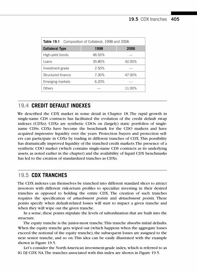
405
19.4 CREDIT DEFAULT INDEXES We described the CDX market in some detail in Chapter 18. The rapid growth in single-name CDS contracts has facilitated the evolution of the credit default swap indexes (CDXs). CDXs are synthetic CDOs on (largely) static portfolios of single-name CDSs. CDXs have become the benchmark for the CDO markets and have acquired impressive liquidity over the years. Protection buyers and protection sell-ers can participate in CDXs by trading in different tranches of CDX. This possibility has dramatically improved liquidity of the tranched credit markets. The presence of a synthetic CDO market (which contains single-name CDS contracts as its underlying assets, as noted earlier in the chapter) and the availability of liquid CDX benchmarks has led to the creation of standardized tranches as CDXs.
19.5 CDX TRANCHES The CDX indexes can themselves be tranched into different standard slices to attract investors with different risk-return profi les to specialize investing in their desired tranches as opposed to holding the entire CDX. The creation of such tranches requires the specifi cation of attachment points and detachment points. These points specify when default-related losses will start to impact a given tranche and when they will wipe out the given tranche.
In a sense, these points stipulate the levels of subordination that are built into the structure.
The equity tranche is the junior-most tranche. This tranche absorbs initial defaults. When the equity tranche gets wiped out (which happens when the aggregate losses exceed the notional of the equity tranche), the subsequent losses are assigned to the next senior tranche, and so on. This idea can be easily illustrated with the example shown in Figure 19.5 .
Let’s consider the North American investment-grade index, which is referred to as IG DJ CDX NA. The tranches associated with this index are shown in Figure 19.5 .
Table 19.1 Composition of Collateral, 1998 and 2006
Collateral Type 1998 2006
High-yield bonds 46.50% —
Loans 35.80% 42.00%
Investment grade 2.50% —
Structured fi nance 7.30% 47.00%
Emerging markets 6.20% —
Others — 11.00%
19.5 CDX tranches

406 CHAPTER 19 Structured credit products
The fi rst tranche with an attachment point of zero and a detachment point of 3% is referred to as the equity tranche. The fi rst 3% of the losses in the underly-ing CDX are absorbed by the equity tranche. As the accumulated losses increase, the next senior tranche will start to experience impairment, and so on. There are prespecifi ed attachment and detachment points for each index in the CDX family. The choice of attachment and detachment points determines the number of slices (or tranches) that will be available to the investors. The greater the subordination levels, the safer will be the super-senior and junior super-senior tranches, and they will tend to attract higher rating and hence will sell for lower spreads.
For example, the Dow Jones iTraxx index has 125 underlying reference names and is a popular CDX index in Europe. Its tranches and their spreads were reported as shown in Table 19.2 .
Note that the tranches that enjoy greater protection from subordination enjoy lower spreads and higher ratings. What factors determine the market spreads? In general, when defaults occur in the underlying single-name CDS contracts of a CDX,
Super senior trancheover 30%
Junior super senior tranche15% to 30%
Senior tranche10% to 15%
Senior mezzanine7% to 10%
Junior mezzanine3% to 7%
Equity tranche0% to 3%
FIGURE 19.5
CDX Tranches (Hypothetical)
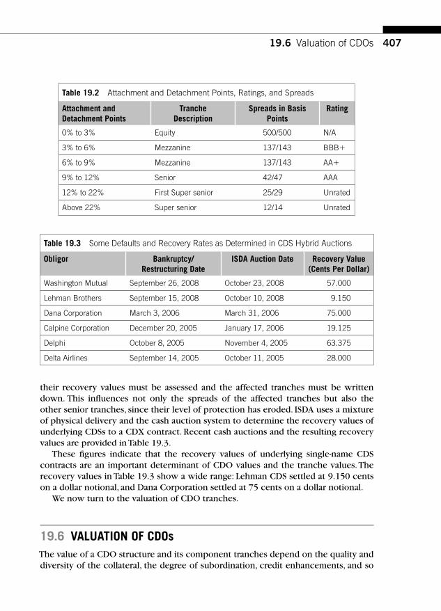
407
their recovery values must be assessed and the affected tranches must be written down. This infl uences not only the spreads of the affected tranches but also the other senior tranches, since their level of protection has eroded. ISDA uses a mixture of physical delivery and the cash auction system to determine the recovery values of underlying CDSs to a CDX contract. Recent cash auctions and the resulting recovery values are provided in Table 19.3 .
These fi gures indicate that the recovery values of underlying single-name CDS contracts are an important determinant of CDO values and the tranche values. The recovery values in Table 19.3 show a wide range: Lehman CDS settled at 9.150 cents on a dollar notional, and Dana Corporation settled at 75 cents on a dollar notional.
We now turn to the valuation of CDO tranches.
19.6 VALUATION OF CDOs The value of a CDO structure and its component tranches depend on the quality and diversity of the collateral, the degree of subordination, credit enhancements, and so
Table 19.2 Attachment and Detachment Points, Ratings, and Spreads
Attachment and Detachment Points
Tranche Description
Spreads in Basis Points
Rating
0% to 3% Equity 500/500 N/A
3% to 6% Mezzanine 137/143 BBB�
6% to 9% Mezzanine 137/143 AA�
9% to 12% Senior 42/47 AAA
12% to 22% First Super senior 25/29 Unrated
Above 22% Super senior 12/14 Unrated
Table 19.3 Some Defaults and Recovery Rates as Determined in CDS Hybrid Auctions
Obligor Bankruptcy/Restructuring Date
ISDA Auction Date Recovery Value (Cents Per Dollar)
Washington Mutual September 26, 2008 October 23, 2008 57.000
Lehman Brothers September 15, 2008 October 10, 2008 9.150
Dana Corporation March 3, 2006 March 31, 2006 75.000
Calpine Corporation December 20, 2005 January 17, 2006 19.125
Delphi October 8, 2005 November 4, 2005 63.375
Delta Airlines September 14, 2005 October 11, 2005 28.000
19.6 Valuation of CDOs

408 CHAPTER 19 Structured credit products
on, as noted earlier. From the perspective of simple valuation models, the valuation is assumed to depend on three critical variables. They are (a) the probability of default of each of the underlying single-name CDSs, (b) the recovery rate on each underlying CDS, conditional on default, and (c) the extent to which defaults in the underlying single-name CDS are correlated with each other. Though the role of probability of default and recovery rates in the valuation is relatively clear cut, the effect of correla-tion on valuation may be less transparent. This is due to the fact that when the cor-relation of defaults is high, it implies that the underlying reference single-name CDS contracts have tendency to default together or survive together.
In a hypothetical CDO with 10 names, the probability distribution of the number of defaults may cluster around 10 or 0 when the correlation coeffi cient is close to 1. In contrast, if the correlation is 0, the default probability may peak around 2 to 3. If the equity tranche were to get wiped out with one default, the latter scenario (with zero correlation) is bad for equity tranche, and the fi rst scenario (with high correla-tion) also implies a higher survival possibility for the equity tranche.
This concept is illustrated in Figure 19.6 . Note that in a simulation involving 5000 paths (with an assumed probability of default of 20%), the equity tranche experi-ences no defaults in nearly 90% of the paths when the correlation is 1! On the other hand, the equity tranche also experiences the maximum number of defaults when the correlation is 1. This might not be nearly as important if we assume that the equity tranche is likely to be wiped out with two defaults, because any outcome over two defaults is only a matter of consequence to other senior tranches in the CDO structure.
4,000
3,500
3,000
2,500
2,000
1,5001,000
500
0
Fre
quen
cy
0 1 2 3 4 5 67 8 9 10Number of defaults
High correlation (99%) Medium correlation (50%) Zero correlation (0%)
FIGURE 19.6
Effect of Correlation on Losses to the Number of Defaults

409
Hence, models of CDO attempt to capture this through simulation methods. To appreciate the valuation method, we briefl y describe a simple model known as the Gaussian Copula, which is intended to serve more as a pedagogical tool than a prac-tical approach. This approach requires us to specify the following items: (a) the sur-vival probability of each CDS contract, (b) the recovery rates associated with each CDS contract, and (c) the correlation of defaults. Given a survival probability, these valuation models transform that information into a distribution of the time when default will occur. This information is then used through a simulation approach to determine the value of each tranche. A discussion of this procedure can be found in Duffi e and Singleton (2003) and other sources. 1 Briefl y, these procedures develop the solution to the valuation of CDOs in a sequential fashion:
1. Simulation of times to default. The survival probability information of each CDS in the synthetic CDO is translated into time to default distribution. In the context of simulation, each path (or scenario) will produce a certain time to default for each name. Consider the following hypothetical CDO with fi ve sin-gle-name CDS contracts. In the various scenarios, times to default may appear as shown in six simulated paths. Let’s assume that all CDS contracts have a recovery value of 40 cents on $1 par value. The data generated in Table 19.4 will take into account different correlations of default.
2. Distribution of losses over time for each tranche. Based on these data, we can see that the equity tranche will experience a loss of 60 cents on a $1 par in PATH 2 after 4.5 years from CDS 3. It will also experience a loss of 60 cents from CDS 4 in PATH 2 after 4.8 years. The notional amount of equity tranche would already have been reduced at Year 4.5 by the loss from CDS 3, so that the loss from CDS 4 at Year 4.8 will further reduce its par value. This way, we
Table 19.4 Simulation of Times to Default of Underlying CDS Contracts
Single-Name CDS in the CDO
Time to Default in
YearsPATH 1
Time to Default in
YearsPATH 2
Time to Default in
YearsPATH 3
Time to Default in
YearsPATH 4
Time to Default in
YearsPATH 5
Time to Default in
YearsPATH 6
CDS 1 10.2 9.7 12.6 11.5 8.2 7.5
CDS 2 19.7 17.2 15.7 18.0 14.3 12.5
CDS 3 5.9 4.5 7.2 8.9 3.8 5.9
CDS 4 7.5 4.8 4.2 7.9 5.9 9.4
CDS 5 9.8 8.2 6.7 10.2 11.9 10.2
1 Duffi e and Singleton, “ Credit Risk: Pricing, Measurement, and Management. ”
19.6 Valuation of CDOs

410 CHAPTER 19 Structured credit products
can determine path by path the time taken for different tranches to be either totally or partially wiped out. Moreover, we can use the simulated losses over time in each path to determine the present value of losses in each path.
3. Determining the required compensation for tranche investors. Then pay-ments to each tranche investor will have to be determined in each path such that the average of the present value of all losses is set equal to the average of the present value of the payments received by the tranche investors. Tens of thousands of paths will be used in practice to determine the valuation of each tranche in the CDO. The valuation will be very sensitive to assumptions made in the model about the correlation of defaults, survival probabilities, and recovery rates. In addition, the specifi c model used to translate survival probabilities into a distribution of time to default will also be an important consideration.
SUGGESTED READINGS AND REFERENCES CDO handbook. Global Structured Finance Research, CDO Research, J. P. Morgan Securities,
April 2002.
Correlation primer. Nomura Fixed Income Research, Nomura , August 2004.
Introduction to the credit derivative indices . Dow Jones CDX and iTraxx, Markit, August 2005.
Duffi e , D. , & Singleton , K. ( 2003) . Credit risk: Pricing, measurement, and management . Princeton, NJ : Princeton University Press .
Mahadevan , S., Tirupathur , V. , Polanskyi , P. , Naraparaju , P. , & Sheets , A. ( 2007) . Structured credit insights ( 3rd ed. ) . Morgan Stanley .

411
100% FHA experience The probability that a loan will be retired during any given year under assumption that the conditional monthly probabilities within each year are constant.
100% PSA convention Assumes that 0.2% of the principal is paid in the fi rst month and will increase by 0.2% in each of the following months, fi nally leveling out at 6% until maturity.
Accrued interest The coupon income that accrues from the last coupon date to the settlement date of the transaction.
Adjustable-rate mortgage (ARM) A mortgage in which the interest rates are linked to certain indexes of borrowing rates and change over the life of the contract.
Adjusted maturity date The maturity date of the bond, rounded down to the nearest quarter from the fi rst day of the maturity month of a Treasury futures contract.
Annual percentage rate (APR) The effective rate charged by lenders. Arbitrage CDO transactions Transactions that attempt to exploit the possibility of selling CDO
liabilities (senior debt, mezzanine debt, and equity) at a higher price to fund the underlying col-lateral pool and have some surplus left over.
Ask price The price at which the market maker is prepared to sell a security. Asset swap A strategy that combines an existing asset with a swap to create a different risk-return
profi le. Asset-backed security (ABS) A type of debt security that is based on pools of assets or is collater-
alized by the cash fl ows from a specifi ed pool of underlying assets. Assumable mortgage A mortgage that can be assumed by the next family that moves into a home
if the previous family moves out. Attachment point The level of default-related losses after which default-related losses will start to
impact a given tranche. Barbell position A long position in a portfolio of two debt securities with one short-term balloon
payment and one longer-term balloon payment. Basis after carry (BAC) The difference between the forward price of the bond and the invoice
price in government futures contracts. Basis in T-bond futures The difference between the fl at (clean) price of the deliverable T-note
and its conversion factor times the futures price. Bid price The price at which the market maker is prepared to buy the security. Bid-cover ratio The ratio of the bids received to the amount awarded or supplied in an auction. Bond covenant An agreed action to be undertaken as well as an agreement not to take certain
actions by the bond issuer and the bond holder. Break-even infl ation (BEI) The infl ation rate under which TIPS perform exactly the way nominal
debt does. Bullet security A debt security that just pays coupons and matures on a specifi c date, with no call
features. Butterfl y strategy A strategy in which an intermediate maturity security is sold (bought) and two
securities for which maturities straddle the intermediate maturity are bought (sold).
Glossary of fi nancial terms
Fixed Income Markets and Their DerivativesCopyright 2009 by Academic Press. Inc. All rights of reproduction in any form reserved.

412 Glossary of fi nancial terms
Call option on yield An option that provides positive cash fl ow if underlying interest rates go up. Callable debt A debt contract that allows the issuer to buy back the debt issue at prespecifi ed
future times at a schedule of call prices. Cap on LIBOR Long position in a put option on Eurodollar futures. Cap pays when LIBOR exceeds
the strike rate specifi ed in the cap. Cash CDO A CDO in which the underlying collateral is made up of cash assets such as bonds and loans. Cash-and-carry arbitrage A situation in the fi nancial markets when the price at which an investor
can sell a bond in the forward market (at the maturity date of the forward contract) is higher than the cost of fi nancing the bond for delivery.
Cash-fl ow CDOs Cash CDOs in which the cash fl ows generated by the underlying collateral pool are suffi cient to pay the promised coupon and principal obligations of CDO debt tranches.
CDO See Collateralized debt obligation. CDS Credit Default Swaps Contracts in which one party (seller of protection) protects another party
(buyer of protection) from the credit risk of a specifi ed obligor, for a specifi ed period of time. CDS spread T he premium paid by the protection buyer to the seller in CDS. CDX See Credit default swap index. CF See Conversion factor. Cheapest to deliver (CTD) See Cheapest to deliverable issue (CDI). Cheapest to deliverable issue (CDI) T he issue that has the lowest basis after carry. Clean price of a T-note or T-bond See Quoted price of a T-note or T-bond. Clearinghouse An organization that monitors the performance of participants through the system
of marking to market, margins, and margin calls that force the participants to respond daily to adverse price movements.
CLN See Credit-linked note. COLA See Cost-of-living adjustment. Collars on LIBOR Long position in a put option and short position in a call option on Eurodollar
futures. Collateral manager A n institution that is responsible for buying assets and managing them as per
the guidelines specifi ed. Collateralized debt obligation (CDO) A debt obligation backed by pools of corporate bonds,
bank loans, and so on. Commercial paper A short-term corporate debt issue. Competitive bid A bid in which bidders specify the quantity that they would like to buy and the
price at which they would like to buy. Compound interest Interest payments depend on frequency of compounding. Calculations vary
with respect to the number of compounding intervals used in any given period. Constant proportional prepayments rate (CPR) Probability that a mortgage will be prepaid
following the next month’s scheduled payments is constant. Consumer Price Index (CPI) An index produced by the U.S. Bureau of Labor Statistics that mea-
sures the average change in prices over time in a fi xed market basket of goods and services. See www.bls.gov/CPI/ for details.
Conversion factor (CF) The price of the delivered bond ( $1 par value) to yield 6%, using certain market conventions.
Convertible security A security that can be converted into a prespecifi ed number of shares of common stock of the issuing company.
Convexity adjustment A n adjustment that is required if one values swaps using ED futures; swaps are like par bonds, and therefore they have convexity, but ED futures settle to LIBOR linearly.
Convexity of a bond T he change in the slope of the price-yield curve for a small change in the yield. Corporate bond A long-term corporate debt issue. Cost-of-living adjustment (COLA) An escalator clause in contracts that provides automatic wage
increases to cover the rising cost of living due to infl ation.

413Glossary of fi nancial terms
Coupon The contractual interest obligation of a bond issuer, which is to be paid to its debt holders. CPI See Consumer Price Index. CPR See Constant proportional prepayments rate. Credit default swap index (CDX) A portfolio of single-name default swaps. Credit event Events such as Chapter 11, Chapter 7, restructuring, and so on are called credit
events. These events will negatively affect the payoffs of the creditors. They are specifi ed in CDS contracts.
Credit-linked note (CLN) Similar to CDS except that the protection buyer receives collateral (by way of the proceeds of CLN issue) at the time the transaction is initiated.
Credit risk Represents a risk that the issuer may be unable to service all or some of the promised obligations due to fi nancial distress, reorganization, workouts, or bankruptcy.
Credit risk puzzle The inability of credit risk models to explain observed credit spreads. Credit spread T he spread between yields of two securities that are identical in all respects except
for their credit quality rating. In practice, spreads of credit-risky debt are calculated with respect to a benchmark such as Treasury or interest rate swap rates.
Cubic spline procedure A smooth curve-fi tting procedure that assumes that the par bond yield is a polynomial function in maturity.
Current yield of a bond A bond’s dollar coupon divided by its price. Market conventions allow the use of clean price or dirty price in the calculation of current yield.
Curvature risk T he risk of realizing losses due to changes in the shape of the yield curve. Dated date The date when the fi rst coupon starts to accrue. DD See Distance to default. Deal spread T he spread on the CDX that is determined at the time they are put together. Dealer A n institution that handles transactions for its customers and purchases securities for its
own account, selling them to customers. Debentures An unsecured bond. The defi nition of this term is different in the United Kingdom. Default A ny missed or delayed disbursement of contractual obligations (interest, sinking funds, or
principal), bankruptcy, receivership, or distressed exchanges. Default-free security A security that is believed to make the promised payments without any
doubt. In other words, the probability of default is zero. Deliverable grade T he minimum quality that the delivered product must achieve when a futures
contract is settled. This concept is especially relevant for futures contracts on sovereign debt and in some CDS contracts.
Delivery options Flexibilities of a seller of a T-note or T-bond futures contract. For example, the quality option, the wildcard delivery option, or the end-of-the-month option.
Detachment point Specifi es when default-related losses will wipe out the given tranche. Dirty price See Invoice price. Discount mortgages Mortgages in which the contractual interest rate is lower than the prevailing
or going mortgage interest rate. Discount window of the Federal Reserve A mechanism through which the central bank lends
funds to depository institutions as a “lender of last resort. ” The rate charged on such loans is known as the discount rate and is a penalty rate with a spread over the target Fed funds rates.
Discriminatory auction A n auction in which the most aggressive bids will be fi lled fi rst at the price at which they were bid, followed by the next aggressive bid, and so on.
Distance to default (DD) The distance between the value of the assets of the fi rm and the face value of debt, standardized in terms of the volatility of the asset value.
Dollar value of an 01 (DV01) T he price change in debt securities for a basis point or 0.01% change in interest rates.
Down-and-out option An option that is very similar to a regular call option except that it auto-matically expires when the underlying asset reaches a prespecifi ed low value.
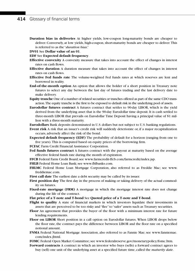
414 Glossary of fi nancial terms
Duration bias in deliveries At higher yields, low-coupon long-maturity bonds are cheaper to deliver. Conversely, at low yields, high-coupon, short-maturity bonds are cheaper to deliver. This is referred to as the “duration bias .”
DV01 See Dollar value of an 01. EDF See Expected default frequency. Effective convexity A convexity measure that takes into account the effect of changes in interest
rates on cash fl ows. Effective duration A duration measure that takes into account the effect of changes in interest
rates on cash fl ows. Effective Fed funds rate The volume-weighted Fed funds rates at which reserves are lent and
borrowed in reality. End-of-the-month option An option that allows the holder of a short position in Treasury note
futures to select any day between the last day of futures trading and the last delivery date to make delivery.
Equity tranche One of a number of related securities or tranches offered as part of the same CDO trans-action. The equity tranche is the fi rst to be exposed to default risk in the underlying pool of assets.
Eurodollar futures contract A futures contract that settles to 90-day LIBOR, which is the yield derived from the underlying asset that is the 90-day Eurodollar time deposit. It is cash settled to three-month LIBOR that prevails on Eurodollar Time Deposit having a principal value of $1 mil-lion with a three-month maturity.
Eurodollars Bank deposits denominated in U.S. dollars but not subject to U.S. banking regulations. Event risk A risk that an issuer’s credit risk will suddenly deteriorate or, if a major recapitalization
occurs, adversely affect the risk of the bond. Expected default frequency (EDF) T he probability of default for a horizon (ranging from one to
fi ve years). This is computed based on equity prices of the borrowing fi rm. FCFAC Farm Credit Financial Assistance Corporation. Fed funds futures contract A futures contract with the payout at maturity based on the average
effective federal funds rate during the month of expiration. FFCB Federal Farm Credit Board; see www.farmcredit-ffcb.com/farmcredit/index.jsp. FHLB Federal Home Loan Bank; see www.fhlbanks.com. FHLMC Federal Home Loan Mortgage Corporation, also referred to as Freddie Mac; see www.
freddiemac.com. First call date The earliest date a debt security may be called by its issuer. First position day The fi rst day in the process of making or taking delivery of the actual commod-
ity on futures. Fixed-rate mortgage (FRM) A mortgage in which the mortgage interest rate does not change
during the life of the contract. Flat price of a T-note and T-bond See Quoted price of a T-note and T-bond. Flight to quality A state of fi nancial markets in which investors liquidate their investments in
assets that are perceived to be too risky and “fl ee ” to “safer ” assets such as Treasury securities. Floor An agreement that provides the buyer of the fl oor with a minimum interest rate for future
lending requirements. Floor on LIBOR Short position in a call option on Eurodollar futures. When LIBOR drops below
the fl oor rate, the contract pays the difference between LIBOR and the fl oor rate on a specifi ed notional amount.
FNMA Federal National Mortgage Association, also referred to as Fannie Mae; see www.fanniemae.com/index.jhtml.
FOMC Federal Open Market Committee; see www.federalreserve.gov/monetarypolicy/fomc.htm. Forward contracts A contract in which an investor who buys (sells) a forward contract agrees to
buy (sell) one unit of the underlying asset at a specifi ed future time, called the maturity date.

415Glossary of fi nancial terms
Forward rates of interest Between two future dates j and k ( k j), a currently agreed-upon rate at which one may borrow or lend on date j for a loan maturing on date k.
Forward swap An interest rate swap in which the fi rst reset date is after the settlement date on which the swap contract is initiated.
Frequency of the swap see Reset period of the swap. FRM See Fixed-rate mortgage. Futures contracts A contract in which an investor who takes a long (short) position in a futures
contract agrees to buy (sell) specifi ed units of the underlying asset (or its cash value) on a spec-ifi ed maturity date at a currently specifi ed futures price. As the contract matures, the investor must make or receive daily installment payments toward the eventual purchase of the underly-ing asset. This practice is known as daily marking to market.
FX risk The risk of realizing losses due to changes in the exchange rate. Gain from convexity The positive price change adjustment of a debt security that corresponds to
the convexity. GC See General collateral. General collateral (GC) repo contract A repo contract in which the lender of cash is willing to
accept any security within a class of securities as collateral and lend cash. General collateral (GC) repo rate The interest rate on a GC repo contract. Generic swap A swap contract in which typically the fl oating index is three-month LIBOR, the
reset date precedes the payment date by exactly the index maturity, and the settlement date is the fi rst reset date.
GIC See Guaranteed investment contract. GNMA Government National Mortgage Association (also referred to as Ginnie Mae; see www.
ginniemae.gov. Guaranteed investment contract (GIC) A debt instrument issued by an insurance company; GIC
guarantees the interest rate payment but not the principal payment. IDB See Interdealer broker. Implied LIBOR Implied LIBOR any day is 100 minus the Eurodollar futures (settlement) price on
that date. Implied repo rate The internal rate of return associated with the strategy of selling T-bond futures
and borrowing and buying an eligible T-bond and delivering it to the futures market at maturity. Implied zeroes Estimates of zero coupon bond prices that are implied by coupon bond prices. Index amortizing swap A transaction in which the notional principal is amortized to precisely
mirror a particular asset’s remaining principal amount. Index maturity of the swap T he underlying LIBOR maturity. Indexing The cash fl ows of the bonds (such as coupons and principal payments) are tied to some
underlying index. Infl ation bond (I-bond) A bond with indexed to infl ation (such as TIPS) earnings; I-bonds are
exempt from local and state taxes. They may have trading restrictions. Infl ation risk The risk of realizing negative changes in the real return after adjusting for infl ation. Interbank markets Markets in which fi nancial institutions lend and borrow between and among
themselves. Interdealer broker (IDB) An institution that aggregates information about the bids and offers posted
by various dealers and disseminates that information on computer screens, without revealing the identities of the dealers. IDBs such as ICAP and eSpeed provide electronic trading platforms.
Interest coverage ratio Interest income from “performing assets ” in the underlying pool divided by the promised interest payments.
Interest rate cap An instrument that caps future interest rate obligations at a predetermined rate for a prespecifi ed period of time.
Interest rate risk The risk that a security’s value will change due to a change in interest rates.

416 Glossary of fi nancial terms
Interest rate swap contract A contract in which two parties agree to make periodic payments to one another computed on the basis of specifi c interest rates on a notional principal amount.
Investment-grade debt A debt that is associated with high-quality notes or bonds that are least likely to default. Rating agencies have specifi c letters for describing investment-grade debt of varying credit quality.
Invoice price in cash markets The price that the buyer of a security has to pay. Invoice price in futures markets The futures settlement price times a conversion factor plus
accrued interest. ISDA International Swap and Derivatives Association; see www.isda.org. Issuer A n entity that sells a fi nancial claim in the marketplace. LBO See Leveraged buyout .Level risk T he risk of realizing losses due to changes in the levels of interest rate. Leveraged buyout (LBO) A transaction used to take a public corporation private that is fi nanced
mainly through debt. LIBID The London Interbank Bid Rate that refl ects the rate at which the banks take loans from
their member banks. LIBOR The London Interbank Offered Rate that refl ects the rate at which the banks offer loans to
their member banks. LIFFE The U.K. government bond contract. Liquidity factor Refl ects the extent of search costs associated with buying or selling a security in
secondary markets. In Treasury markets, the yield spread between on-the-run and off-the-run Treasury is a measure of liquidity risk.
Liquidity measure A measure of the ability to buy or sell large amounts of a security easily at a narrow bid-offer spread without an adverse price reaction.
Liquidity risk The risk that arises from the diffi culty of selling or buying an asset in a timely manner.
Loan-to-value ratio (LTV) The initial borrowed amount divided by the value of the property. Location option An option that is imbedded in futures contracts and permits the short some fl ex-
ibility in the choice of the location of physical delivery. Lognormally distributed random variable A random variable, the natural logarithm of which is
normally distributed. Loss given default The amount that would be lost if a counterparty defaults. LTV See Loan-to-value ratio. Macaulay duration of a debt security Its discounted-cash-fl ow-weighted time to receipt of all its
promised cash fl ows divided by the price of security. Maintenance margin The lowest balance of funds that is allowed when trading on margin. Margin An amount that is set aside to ensure that the investor has suffi cient equity to meet any
adverse price moves. Margin call A requirement to restore the margin level to the initial margin level by posting cash. Market capitalization The total dollar value of all outstanding securities. Market price of an asset The amount of money that a willing buyer pays to acquire the asset
from a willing seller when a buyer and seller are independent and when such an exchange is motivated by only commercial consideration.
Market value CDOs Cash CDOs in which the fund manager is allowed to trade the underlying col-lateral more so as to maintain the market value of the collateral at a level that is more than suf-fi cient to pay the promised obligations of CDO debt tranches.
Marking to market T he process of determining the daily installments by the daily change in the futures price: If the futures price goes up, the investor who is long in the futures contract receives a payment, that equals the change in the daily futures price, from the investor who is short.
MATIF France’s futures exchange; see www.matif.fr.

417Glossary of fi nancial terms
Matrix price The price that is derived based on theoretical models and is provided by bond-pricing fi rms such as Datastream, IDC, etc.
Maturity date The date on which the bond matures and is paid off in full. MBS See Mortgage-backed security. MEY See Mortgage-equivalent yield. Mezzanine tranche One of a number of related securities or tranches offered as part of the same
transaction. The mezzanine tranche investors are protected by equity investors against default and recovery risks.
Migration probability The probability that a given fi rm may move from one category of rating into another category.
Modifi ed duration The percentage change in price of the security for a change in yield of the security.
Mortgage-backed security (MBS) Bond that is secured or backed by a portfolio of underlying mortgage loans.
Mortgage-equivalent yield (MEY) A yield that is quoted in annualized terms, assuming monthly compounding.
Mutual fund Pool of money that is managed by an investment company. Net basis See basis after carry. Netting by novation A contract between two counterparties under which any obligation to
each other to deliver a given currency on a given date is automatically amalgamated with all the other obligations for the same currency and value date, legally substituting one single-net amount for the previous gross obligations.
Noncompetitive bid A bid in which bidders can specify the amount that they would like to buy but do not specify the price.
Noninvestment grade debt A debt that is associated with low-quality notes or bonds that are more likely to default compared to investment-grade debt. Rating agencies assign letters to classify different groups of noninvestment-grade debt.
OAS See Option-adjusted spread . Offset An investor who is short in a futures contract takes an equal amount of long position in the
same futures contract and closes out his position. OIS See Overnight index swaps. On-the-run issue A newly auctioned security. Operating risk T he risk of the underlying business. Option-adjusted spread (OAS) A change of the discount rate that is required to equalize the aver-
age present value across all simulated paths (model price) to the market price. Overnight index swaps (OIS) A swap in which one party agrees to pay fi xed and the other party
agrees to pay a fl oating interest rate that is tied explicitly to a published index of a daily over-night rate benchmark, such the overnight Fed funds rate.
PAC structure A structure in which the tranches are created to provide varying levels of protec-tion from the risk of prepayments.
Par bond yield curve The relationship between the yield to maturity and time to maturity of bonds that sell at their par value.
Payment lag The time lag between the reset date and the payment date. Pool factor T he outstanding mortgage pool principal divided by the original principal balance,
expressed as a decimal between 0 and 1. Post-trade transparency of a market The availability of information that investors will have
about most recent trades and that will help them evaluate the quality of execution of trades relative to recently concluded trades.
Premium mortgage A mortgage in which the contractual interest rate is greater than the prevail-ing or going mortgage interest rate.

418 Glossary of fi nancial terms
Prepayment A borrower’s choice to refi nance previously taken loans. Pretrade transparency in a market The availability of information that serves to reduce the
search costs to potential investors by providing them, in one screen, with a complete picture of trading opportunities, not just with one dealer but with multiple dealers.
Price limits Limits that stipulate the range of futures prices within which trading will be sustained in the futures markets.
Price value of a basis point (PVBP) See Dollar value of an 01 (DV01). Primary dealers Banks and securities brokerages that trade in U.S. government securities with the
Federal Reserve System. Primary debt market A market where borrowers issue debt securities to raise capital. Primary mortgage market A market where borrowers get their loans from lenders. Process of securitization T ransformation of illiquid, individual mortgages into liquid mortgage-
backed securities. PSA Public Securities Association; see www.psa.com. Puttable bond A bond that allows the investor to sell the bond back to the issuer, prior to maturity,
at a price that is specifi ed at the time that the bond is issued. PVBP See Price value of a basis point. Quality option An option that allows the short to deliver any bundle of prespecifi ed Treasury
notes or bonds sometime during the delivery month, so long as the investor has not offset his or her short position.
Quoted price of a T-note or T-bond T he dirty price minus the accrued interest. Rating agency A n agency that provides information about the borrower’s fi nancial health. Recovery rate The amount that will be paid on a dollar if there is default. Reduced-form model A way to model default risk in which default arrival times and recovery
rates conditional on defaults are specifi ed exogenously. Reinvestment risk The risk of realizing losses due to changes in the future interest rates. REMICs Real Estate Mortgage Investment Conduits, introduced in the Tax Reform Act of 1986, are
a type of special-purpose vehicle used for the pooling of mortgage loans and issuance of mort-gage-backed securities.
Repo agreement A contract in which a security is sold with an agreement on the initiation date to repurchase the security at a higher price on a later date specifi ed in the contract.
Reserve requirements The percentage of deposits that a depository institution must maintain either as cash or on deposit at a Federal Reserve Bank.
Reset period of the swap The frequency with which the fl oating leg of the swap is reset. Residual claim A claim to a share of earnings once all the company’s prior-ranking obligations
have been discharged. Reversed repo agreement A contract in which a security is borrowed with an agreement on
the initiation date to replace the security at a higher price on a later date specifi ed in the contract.
Risk of infl ation The risk of realizing losses due to unanticipated infl ation. Risk premium The difference between the at-issue bond interest rate and the risk-free rate. Safety covenants Covenants that are specifi ed to protect bondholders. Sealed-bid auction Bidders cannot see other bidder’s choices and must form expectations about
where other bidders might bid. Seasoning ramp Prepayments are higher when the life of the loan is in the range of two to eight
years, and then the prepayments stabilize. Secondary debt market A market in which securities are traded after they are initially offered in
the primary market. Secondary mortgage market A market where mortgages that were previously originated are
bought and sold.

419Glossary of fi nancial terms
Senior tranche One of a number of related securities or tranches offered as part of the same transaction. The senior tranche investors are protected by both equity and mezzanine investors.
Sequential structure A structure in which specifi c rules dictate how the cash fl ows (including prepayments) from the collateral are allocated to each tranche.
Settlement date A date when the buyer and seller exchange cash and security as per the terms agreed upon on the pricing date.
Simple interest Interest calculations don’t vary with respect to the number of compounding inter-vals used in any given period.
Single monthly mortality (SMM) rate A probability that the mortgage will be prepaid following the fi rst month.
Single-name credit default swap (CDS) A n over-the-counter (OTC) contract that allows one party to sell insurance on a named debt obligation to another party.
Sinking fund provision A provision that requires the issuer of an indenture to retire a specifi ed portion of debt each year.
SLMA Student Loan Marketing Association, also referred to as Sallie Mae; see www.slma.org. Slope risk T he risk of realizing losses due to changes in the slope of the yield curve. SMM See Single monthly mortality (SMM) rate. Sovereign debt A debt instrument guaranteed by a government. Special collateral repo contract A contract in which the lender of funds specifi es a particular
security as the only acceptable collateral. Special-purpose vehicle (SPV) A legal entity created to receive specifi c assets from the fi nancial
institution; bankruptcy of the fi nancial institution will not affect the cash fl ows of assets placed in the SPV.
Special repo rate The rate on the special collateral repo contract. Spot curve T he relationship between the spot rate (yield to maturity) of a pure discount bond and
its maturity. Spot rate of interest The yield to maturity on a default-free zero coupon (pure discount) bond. Spread duration T he sensitivity of the price of a bond to a 100-basis-point change to its option-
adjusted spread. Stop-out yield The yield at which the aggregate demand exhausts the supply to the competitive tender. Strategic debt service Bondholders may get less than what was promised when there are costs to
fi nancial distress and when borrowers have some bargaining power. Strip of futures A portfolio of futures contracts. STRIPS (Separate Trading of Registered Interest and Principal Securities) Securities that
may be maintained in the book-entry system operated by the Federal Reserve Banks in such a way that it is possible to trade, in book-entry form, interest and principal components as direct obligations of the U.S. Treasury.
Structural model A theoretical model that specifi es the circumstances under which defaults may occur and the rights and responsibilities of borrowers and lenders when default occurs.
Subordinated corporate debt A debt that is repayable only after other debt issues senior to it have been repaid.
Superpoison put provision A provision that requires from the sellers of bonds a right that allows the investors to sell (or put) the bonds back to the seller at par value when the credit quality of the issuer deteriorates.
Swap rate T he fi xed rate that is paid on the same dates as the fl oating payments with a present value equal to that of the fl oating payments.
Swap spread The difference between the fi xed rate on a swap and the yield of the underlying Treasury benchmark with the same maturity.
Swaption An option that gives the right to enter into a swap at a future date at terms that are agreed upon now.

420 Glossary of fi nancial terms
Synthetic CDO A CDO in which the underlying collateral itself is a portfolio of credit default swaps .
TAC (targeted amortization class) CMOs CMOs that are similar to PAC CMOs. However, the TAC CMOs have a longer average maturity when interest rates fall, and the prepayments are slower.
TAF (term auction facility) The facility whereby banks are able to borrow from the Fed for a term of approximately one month by posting a broad menu of collateral.
Target Fed funds rate An overnight (policy) interest rate that is announced by the Fed based on its analysis of the economy. The Fed uses its monetary policies to keep the short-term interest rates close to the announced target rate.
Tax risk An uncertainty regarding tax status of debt security that was originally issued with certain tax exemption features.
TBA (to be announced) trade T rade that occurs before key features of the underlying pool become available.
TED spread Spread between the Eurodollar futures rate and the T-bill rate. Term structure of interest rates The relationship between the yield to maturity of default-free
zero coupon securities and their maturities. Tiered custodial system A system that records the ownership of securities in entries on the
books of a series of custodians. Time to maturity The time remaining until a debt contract expires. Timing option A n option implicit in futures contracts that allows the short to delivery on any
business day of the delivery month, typically with a short notice period. Timing risk The security has an uncertainty about the timing of the cash fl ows. An example would
be mortgages, which have prepayment risks. TIPS Treasury Infl ation-Protected Securities. Trading volume T he number of bonds traded during a given period or the dollar value of the
bonds traded during a given period. Transparency of a market The widespread availability of information relative to current oppor-
tunities to trade and recently completed trades. Treasury bills (T-bills) Treasury securities that are issued by the Treasury with a maturity of less
than or equal to one year at the time of issuance. Such securities do not pay any coupon. Treasury bond futures contracts Futures contracts that have a contract size of one U.S. Treasury
bond having a face value at maturity of $100,000 or multiple thereof. The deliverable grade is U.S. Treasury bonds that, if callable, are not callable for at least 15 years from the fi rst day of the delivery month or, if not callable, have a maturity of at least 15 years from the fi rst day of the delivery month.
Treasury bonds (T-bonds) T reasury securities that pay coupons and that have maturities in excess of 10 years. Currently the Treasury has a 30-year T-bond that is regularly auctioned.
Treasury debt securities The debt securities that are issued by the U.S. Treasury. Treasury note futures contracts Futures contracts that have a contract size of one U.S. Treasury
note having a face value at maturity of $100,000 or multiple thereof. The deliverable grade is U.S. Treasury notes maturing at least 6.5 years, but not more than 10 years, from the fi rst day of the delivery month.
Treasury notes (T-notes) T reasury securities that pay coupons and that have maturities in the range of one to 10 years at the time of issuance.
Trustee An institution that acts as the custodian and performs several key functions: First, the trustee bears responsibility for the safe custody of the assets and for compliance with the guide-lines set forth in the CDO structure. Second, the trustee is also responsible for computing the contractual payments due to the different players in the CDO transaction. Third, the trustee is responsible for keeping the investors informed about the integrity of the CDO.
Uniform price auction A uction in which all the winning bidders pay exactly the same price.

421Glossary of fi nancial terms
Volatility A measure of the variability of interest rates relative to their expected average levels. When-issued (WI) markets Markets in which the bidders can take long or short positions in
the “ to-be-auctioned ” Treasury securities. They would do this prior to bidding in the auction. WI markets allow orderly and credible book building in Treasury securities.
Wild-card delivery option A n option in T-note futures contracts that allows delivery during the delivery month until 8:00 p.m.
Workouts A process that may lead to exchange offers in which old debt contracts are replaced by new debt contracts, which may be less valuable to the creditors.
Yield curve The plot of yield to maturity against time to maturity or against a risk measure. Yield-curve swap A n interest rate derivative, using which counterparties swap yields with differ-
ent maturities. Yield-curve trade A trade that changes the structure of the assets by steepening or fl attening the
interest rate payments. Yield to maturity (YTM) T he internal rate of return (IRR) of the debt security; it is the discount
rate at which the present value of all future promised cash fl ows is exactly equal to its market price.
Yield to worst T he yield that is computed assuming that the bond will be called on each call date, and the highest of the resulting yields is reported as yield to worst.
Z bond tranche A tranche that receives no cash fl ows until all earlier tranches are fully retired.

This page intentionally left blank

423
A Accrued interest , 37 – 38 , 250 , 392
excel functions for , 40
Adjustable-rate mortgage (ARM) , 231 – 233
Agency debt securities , 10 . See also Debt securities
Agency mortgage , 233 . See also Mortgage
Alt-A mortgage , 233 . See also Mortgage
Annual percentage rate (APR) , 237
Annuities, compounding and discounting , 27 – 29
APR. See Annual percentage rate (APR)
Arbitrage, CDO , 400
ARM. See Adjustable-rate mortgage (ARM)
Asset backed securities market (ABS) , 12
Asset swaps , 326 – 327
Asset values, probability distribution of , 220
Attachment point , 402
B BAC. See Basis after carry (BAC)
Balance sheet
CDO , 400
Balloon payment , 7
Bankruptcy
defaults , 199 – 200
Banks. See also Central banks
commercial , 227 , 238 , 267 , 345
investment , 10 , 246 , 248 , 249 , 345
role in debt markets , 11
Basis after carry (BAC) , 369 – 370
BBA. See British Bankers Association (BBA)
BDT model. See Black, Derman, and Toy (BDT) model
BEI. See Break-even infl ation (BEI)
Below investment grade. See Junk grade
Benchmark treasury debt securities auctions ,
87 – 91
BEY. See Bond-equivalent yield (BEY)
Bid-cover ratio , 96
Bid-offer spreads , 347 – 348
trading , 119
Bid shading , 99 – 100
Black, Derman, and Toy (BDT) model , 180 – 188
Black and Cox approach, for subordinated corporate
debt , 216
Black and Schole’s pricing model
value of equity , 206 – 207
Black’s formula for caps , 323
Black’s model , 322
Bond and loan default volumes for 1970 – 2006 ,
198 – 199
Bond-equivalent yield (BEY) , 35 – 36 , 233
Bondholders
probability distribution of payoffs to , 220
Bonds
excel functions for , 39
forward price on bonds using repo markets , 72
Book building in WI market , 93
Bootstrapping , 144 – 150
Break-even infl ation (BEI), TIPS , 270 , 280 – 283
British Bankers Association (BBA) , 303 , 304
Bullet securities , 5
Bullet vs barbell securities , 122 – 125
Business cycles , 197 – 201
Butterfl y trades , 122 – 125
Buyer of protection, CDS , 378 , 380
“ Buy-side ” institutions , 11
C Calibration, to market data , 180 – 188
Callable bond, cash fl ows , 128
Call option , 316
“ Call risk ” , 18
Caps , 317 – 321 , 327
valuation of , 321 – 324
Cash-and-carry arbitrage , 366
Cash-fl ows
of callable bond , 128
CDO , 401
matrix , 147 – 148
MBS , 250 – 251
with prepayments , 254 – 257
mortgage , 233 – 237
rights of debt securities , 7–8
schedule, of coupon bonds , 148
TIPS , 283 – 288
structures , 278 – 280
Cash-fl ow-weighted times , 110
Index

424 Index
Cash management bills (CMBs) , 89
Cash types, CDOs
arbitrage , 400
balance sheet , 400
cash fl ow , 401
market value , 401
Cash yields mortgage , 233–237
CDI. See Cheapest to deliverable issue (CDI)
CDOs. See Collateralized debt obligations (CDO)
CDS. See Credit default swaps (CDS)
CDS contracts
applications , 391–393
entering and closing out , 379
growth of , 380–282
ISDA rules for settling on credit events , 384–386
restructuring , 383–384
trading , 379
CDS spreads , 379–380
pricing , 388
restructuring clause on , 383–384
valuation , 386–391
CDX. See Credit default swap index (CDX)
CDXs. See Credit default indexes (CDX)
Central banks. See also Fed
role in debt markets , 10
Cheapest to deliverable issue (CDI) , 370
Cheapest to deliver (CTD) , 370
Chicago board of trade (CBOT) , 357 , 360
Chicago Mercantile Exchange , 306
CIR model. See Cox, Ingersoll, and Ross (CIR)
model
Clean price. See Quoted price
CLN. See Credit-linked notes (CLN)
CLOs. See Collateralized loan obligations (CLOs)
Collar on LIBOR , 317–321
Collateralized debt obligations (CDOs) , 397–410
balance sheet of , 398
cash types , 400–401
Gaussian Copula model , 409
market growth , 404–405
mezzanine notes , 398
players of , 399–400
senior notes , 398
structure of , 399–400
analysis of , 401–404
subordinated notes , 398
synthetic , 401
trenches , 398–399
valuation of , 407–410
Collateralized loan obligations (CLOs) , 400
Collateral manager , 398
Collateral pool, quality of , 404
Collateral repo auctions, by Fed , 47–48
Competitive bid , 94
Compounding , 25–31
annuities , 27–29
future values , 25–27
present values , 27–29
semiannual , 32–33
Compound-interest calculations , 25–26
Conditional prepayments rate (CPR) , 252
Constant monthly mortality, prepayments ,
251 –252
Consumer Price Index (CPI), TIPS , 275–276
Contracts
CDS. See Contracts
CLN , 393
mortgage , 227–230
OTC. See Over-the-counter (OTC) contracts
Contractual risk, debt security , 18–19
Conversion factor, treasury futures contracts ,
363 –364
Convexity
adjustment , 338–339
of price-yield relation , 42 , 43 , 44
Convexity, DV01 , 119–125
bullet vs barbell securities , 122–125
butterfl y trades , 122–125
effect , 124
estimation , 121
gain , 122
Corporate bonds
selling of , 58–59
Corporate debt , 58–59
Corporate zero coupon bonds , 211
Corporations, role in debt markets , 11
Coupon strips , 156–157
Cox, Ingersoll, and Ross (CIR) model , 178–180
CPI. See Consumer Price Index (CPI)
CPR. See Conditional prepayments rate (CPR)
Credit crunch, of 2007 –2008
Fed actions to stem , 53–56
Fed target rate cuts during , 55
LIBOR versus target Fed funds rate during , 54
Credit default indexes (CDXs) , 405–407
tranches , 405–407
Credit default swap index (CDX) , 394–395 , 405
salient features of , 394
Credit default swaps (CDS) , 277–395 , 401
buyer of protection , 378 , 380

425 Index
credit event, settlement on , 384 – 386
documentation choices in , 382
market growth and evolution , 380 – 382
players , 380
premium , 378
restructuring and deliverables , 382 – 384
seller of protection , 378 – 379 , 381
single-name , 407
valuation of , 386 – 393
applications , 391 – 393
CDS spreads/probability of default/recovery
rates , 388 – 391
Credit enhancement, MBS , 247 – 249
Credit event
CDS settlement on , 384 – 386
defaults , 199
lower recovery rates and , 212 – 213
Credit-linked notes (CLN) , 393
Credit-rating, categories of , 203
Credit risk
in bank sector , 344
debt security , 15 – 16
management , 346 – 347
puzzle , 223
Credit spreads , 200
models of , 223 – 224
CTD. See Cheapest to deliver (CTD)
Cubic spline fi tted yields , 159
Cubic spline procedure , 158
Current yield , 33
DV01 or PVBP with variations around , 109
Customer, primary dealer transactions with , 60
D Dealer market transparency
classifi cation , 61
evidence on trading characteristics , 63 – 64
indicators of , 61 – 63
initiatives to improve , 65
matrix prices and execution costs , 64
Dealers, role in debt markets , 11
Debentures (unsecured debt) , 7
Debt
corporate , 58 – 59
infl ation-indexed. See Infl ation-indexed debt
subordinated corporate , 216
value of corporate, Black and Schole’s pricing
model , 207
Debt at maturity
value of corporate , 205
Debt contracts , 3–7
cash-fl ow rights of debt securities , 7–8
primary and secondary markets , 8
Debt markets , 3
players in , 8 – 12
primary and secondary , 8
role of central banks in , 10
Debt pricing
cost of, Merton’s model , 217 – 220
Debt ratio, defi ned , 208
Debt securities , 3–4. See also Repo contracts
cash-fl ow rights of , 7–8
classifi cation of , 12 – 14 , 203
defaults , 201
federal agency , 242 – 244
option pricing models , 205 – 207
outstanding (1996 and 2007) , 13
risk of , 14 – 21
contractual risk , 18– 19
credit risk , 15 – 16
event risk , 20 , 21
FX risk , 20 – 21
infl ation risk , 19 – 20
interest rate risk , 14 – 15
liquidity risk , 16 – 18
tax risk , 20
treasury. See Treasury auctions
Default , 197 – 201
bankruptcy , 199 – 200
credit event , 199
debt securities , 201
by investment-grade speculative-grade companies ,
197 – 199
rating agencies defi nition of , 197
recession , 200 – 201
risk , 228 – 229
structural models of , 204 – 213
implementation, KMV approach ,
213 – 217
market prices , 212 – 213
probability and loss , 210 – 212
Default-free security , 4 , 5
Default premium
effect of leverage on , 208 – 209
effect of operating risk on , 209
Deliverables, CDS , 382 – 384
Delivery specifi cations , 357 – 358
Detachment point , 402
Dirty price (invoice price) , 34 , 80 – 81
of coupon bonds , 147 – 148

426 Index
Discounting , 25–31
annuities , 27–29
future values , 25–27
present values , 27–29
Discount mortgage , 260
Discount window, of Federal Reserve , 48–49
primary and secondary credit under , 49 , 50
Discriminatory auctions , 97–98
Diverse swap contracts , 328
Diversity score , 404
Documentation choices in CDS , 382
Dollar value of 01 (DV01)
convexity , 119–125
duration. See Duration, DV01
effective convexity , 125–129
effective duration , 125–129
hedging , 118–119
price risk , 105–109
trading , 118–119
Downward-sloping term structure
in CIR model , 180
in Vasicek model , 177
Due diligence , 400
Duration
bias in deliveries , 373
estimates, for treasury benchmarks , 114
versus yield , 140
Duration, DV01 , 109–117
as cash-fl ow-weighted times , 110
effective , 125–129
estimates, for treasury benchmarks , 114
Excel applications , 113–116
Macaulay duration , 109–112
modifi ed duration , 112–113
portfolio duration , 116
as price elasticity of interest rates , 112
properties , 116
DV01. See Dollar value of 01 (DV01)
E ECB. See European Central Bank (ECB)
Economic news announcements, and volatility ,
138 –140
EDF. See Expected default frequency (EDF)
Eligible collateral , 401
End-of-the-month option , 363
EONIA. See Euro Overnight Index Average (EONIA)
Equity prices
Merton’s model implementation using , 214
Equity tranche , 398
Eurodollar
calculating yields in cash market , 305–306
futures contract , 308–311
futures markets , 306–311
Eurodollar futures contract
options on , 316–321
settlement
add-on settlement feature , 309
LIBOR , 308–311
versus swap markets , 315
swap pricing , 336–338
swap rates, deriving , 311–315
Eurodollar markets , 303–306
Eurodollar time deposits (TD) , 303
Euro Overnight Index Average (EONIA) , 297
Europe, tri-party repos in , 86
European Central Bank (ECB) , 45 , 55
Event risk , 5 , 21
debt security , 20
Ex ante , 158
Excel functions
for accrued interest , 40
for bonds , 39
for converting quotes to decimals, and vice versa ,
34
for duration , 113–116
Excel solver
computing yield to maturity using , 41
Excel T-bill functions , 37
Execution costs, market transparency , 64
Expected default frequency (EDF)
KMV approach to calculate , 215
F Fails in repo market , 84 , 85
Fannie Mae. See Federal National Mortgage
Association (FNMA)
Farm Credit Financial Assistance Corporation
(FCFAC) , 238
FCFAC. See Farm Credit Financial Assistance
Corporation (FCFAC)
Fed , 45–46 . See also Central banks
actions to stem credit crunch of 2007 –2008 ,
53 –56
funds rates. See Fed funds rates
major functions of , 46
monetary policies of , 46–51
discount window , 48–49
goals of , 46–51
open market operations , 46–48

427 Index
reserve requirements , 49 – 51
payments systems and conduct of auctions , 53
Federal agencies
debt securities , 242 – 244. See also Debt securities
empirical evidence on spreads , 243 – 244
GSE , 238 – 242
advances , 241
benefi ts to , 241
credit guarantees by , 240
mortgage investments by , 240 – 241
operations for earning money , 240 – 241
mortgage and , 237 – 242
role in debt markets , 10 – 11
Federal Farm Credit Board (FFCB) , 238
Federal Home Loan Bank (FHLB) , 238 – 239
Federal Home Loan Mortgage Corporation (FHLMC) ,
238
guarantees and credit enhancement by , 249
share of purchases of loans by , 239
Federal Housing Administration (FHA)
prepayment risk , 252 – 253
residential mortgage , 238
Federal National Mortgage Association (FNMA) , 238
guarantees and credit enhancement by , 248
share of purchases of loans by , 239
spreads over treasury yields , 243 – 244
Federal Open Market Committee (FOMC) , 45 , 54
Federal Reserve. See Fed
Federal Reserve Bank, New York , 295
Federal Reserve System , 45 , 58
Fed funds futures , 294 – 297
average daily rates , 295
future target rates , 295 – 297
Fed funds rates , 51 – 53
during credit crunch 2007 – 2008 , 55
effective , 52
for fi nancial market stability , 52 – 53
funds transactions , 51
target , 46 , 52
FFCB. See Federal Farm Credit Board (FFCB)
FHA. See Federal Housing Administration (FHA)
FHLB. See Federal Home Loan Bank (FHLB)
FHLMC. See Federal Home Loan Mortgage
Corporation (FHLMC)
Financial distress
cost of, Merton’s model , 217 – 220
fi nancial reorganizations to manage , 219 – 220
Financial institutions
role in debt markets , 11
Financial market stability
Fed funds rates for , 52 – 53
Financial reorganizations
key empirical regularities associated with , 219
to manage fi nancial distress , 219 – 220
Fitted vs actual yields , 163
Fixed-income markets. See Debt markets
Fixed-rate mortgage (FRM) , 230 – 231
Flat price. See Quoted price
Floors , 317 – 321 , 328
FNMA. See Federal National Mortgage Association
(FNMA)
FOMC. See Federal Open Market Committee (FOMC)
Forward contracts , 353 – 355
vs. futures contracts , 359
Forward price , 353 , 369
on bonds using repo markets , 72
Forward rate calculations , 331
Forward rates determination, by no-arbitrage , 152
Forward rates of interest , 151 – 155
determination, by no-arbitrage , 152
locking, by zero coupon bonds , 153
spot rates , 154
zero prices , 154
Forward swap , 334 – 335
Forward trading , 93
Freddie Mac. See Federal Home Loan Mortgage
Corporation (FHLMC)
FRM. See Fixed-rate mortgage (FRM)
Funds transactions, Fed , 51
Futures contract, Eurodollars , 308 – 311
deriving swap rates , 311 – 315
options on
caps , 317 – 321
collar on LIBOR , 317 – 321
fl oors , 317 – 321
settlement , 308 – 311
versus swap markets , 315
swaps pricing , 336 – 338
Futures contracts , 355 – 356
features of
delivery specifi cations , 357 – 358
margins , 358 – 359
price limits , 358
location option , 358
offset , 357
T-bond , 357
timing option , 358
T-note , 360 – 363
treasury , 359 – 375
vs. forward contracts , 359

428 Index
Future values, compounding and discounting , 25–27
FX risk, debt security , 20–21
G Gaussian copula model , 409
General collateral (GC) repo agreement , 77–82
GC repo contract , 77–78
GC repo rates , 78–82
General Motors debt , 5–7
Generic interest rate swap , 329
GIC. See Guaranteed investment contracts (GIC)
Ginnie Mae. See Government National Mortgage
Association (GNMA)
GNMA. See Government National Mortgage
Association (GNMA)
Government National Mortgage Association (GNMA) ,
238
guarantees and credit enhancement by , 248
Governments, role in debt markets , 10
Government-sponsored enterprises (GSE) , 238–242
advances , 241
benefi ts to , 241
credit guarantees by , 240
infl uence on secondary markets for residential
mortgages , 240
mortgage investments by , 240–241
operations for earning money , 240–241
role in debt markets , 10–11
GSE. See Government-sponsored enterprise (GSE)
Guaranteed investment contracts (GIC) , 266
H Haircut , 70
trading , 119
Hedging , 118–119 , 345
applications , 373–375
High-coupon bonds , 373
High-coupon notes , 373
Households
role in debt markets , 11–12
Housing prices, prepayment , 257
Humped yield curve , 134
I IBF. See International Banking Facilities (IBF)
IDB. See Interdealer brokers (IDB)
IMM. See International Monetary Market (IMM)
Implied LIBOR , 309
Implied repo rate (IRR) , 370–373
Implied zeroes , 143–144
Implied zero prices
market prices of strips, and , 161
vs strip prices , 162
Indexation lag, TIPS , 278
Indexed bonds
timing of introduction of , 273
Indexed zero coupon structure, TIPS , 279
Index maturity , 328
Infl ation-indexed debt , 269–273
risk associated with , 275
role of , 273–275
Infl ation-indexed government bond markets
current issuers of , 272
growth of 1997 –2007 , 272
Infl ation risk
debt security , 19–20
premium , 281
Interbank market , 303
Interdealer brokers (IDB) , 59–60
primary dealer transactions with , 60
Interest-indexed structure, TIPS , 280
Interest rates
derivatives , 188–193
empirical evidence on risk structure of , 210
forward , 151–155
future distribution , 126
mean-reverting , 172–180
pattern in 30-year fi xed-rate mortgage , 236
risk , 14–15 , 229–230
simulation , 127
spot rate , 143
term structure , 143–151
volatility , 135–138
Intermarket spreads , 315–316
Internal rate of return (IRR) , 5 , 31–33. See also Yield
to maturity (YTM)
semiannual compounding , 32–33
International Banking Facilities (IBF) , 303
International Monetary Market (IMM) , 306
International Swap and Derivatives Association
(ISDA) , 382–383
rules for CDS settlement on credit events ,
384 –386
Inverse cash-fl ow matrix , 147 , 149
Inverted yield curve , 132 , 133
Investment-grade companies
defaults by , 197–199
Investment grade credit-rating , 203
Investment grade debt , 6
Investors
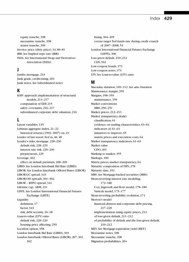
429 Index
equity tranche , 398
mezzanine tranche , 398
senior tranche , 399
Invoice price (dirty price) , 34 , 80 – 81
IRR. See Implied repo rate (IRR)
ISDA. See International Swap and Derivatives
Association (ISDA)
J Jumbo mortgage , 233
Junk grade, credit-rating , 203
Junk notes. See Subordinated notes
K KMV approach, implementation of structural
models , 213 – 217
computation of EDF , 215
safety covenants , 216 – 217
subordinated corporate debt valuation , 216
L Latent variables , 135
Lehman aggregate index , 21 – 22
historical returns (1992 – 2007) on , 23
Lender of last resort, Fed as , 46 , 48
Lender’s risks, mortgage , 228 – 230
default risk , 228 – 229
interest rate risk , 229 – 230
prepayments , 229
Leverage , 402
effect on default premium , 208 – 209
LIBID. See London Interbank Bid Rate (LIBID)
LIBOR. See London Interbank Offered Rates (LIBOR)
LIBOR-GC spread , 343
LIBOR-OIS spreads , 301 – 302
LIBOR – REPO spread , 341
Lifetime cap, ARM , 231
LIFFE. See London International Financial Futures
Exchange (LIFFE)
Liquidity
defi nition , 17
factor , 343
risk, debt security , 16 – 18
Loan-to-value (LTV) ratio
default risk , 228 – 229
housing price affecting , 259
Location option , 358
London Interbank Bid Rate (LIBID) , 303
London Interbank Offered Rates (LIBOR) , 267 , 301 ,
302
fi xing , 304 – 305
versus target Fed funds rate during credit crunch
of 2007 – 2008 , 54
London International Financial Futures Exchange
(LIFFE) , 306
Loss given default , 210 – 212
CDS , 392
Low-coupon bonds , 373
Low-coupon notes , 373
LTV. See Loan-to-value (LTV) ratio
M Macaulay duration , 109 – 112. See also Duration
Maintenance margin , 359
Margins , 358 – 359
maintenance , 359
Market conventions
MBS , 250 – 251
Market prices , 212 – 213
Market transparency, dealer
classifi cation , 61
evidence on trading characteristics , 63 – 64
indicators of , 61 – 63
initiatives to improve , 65
matrix prices and execution costs , 64
Market transparency, indicators , 61 – 63
Market value
CDO , 401
Marking to market , 355
Markups , 100
Matrix prices, market transparency , 64
Maturity composition of TIPS , 278
Maturity date , 353
MBS. See Mortgage-backed securities (MBS)
Mean-reverting interest rate modeling ,
172 – 180
Cox, Ingersoll, and Ross model , 178 – 180
Vasicek model , 175 – 177
Mean-reverting probability evolution , 174
Merton’s model
fi nancial distress and corporate debt pricing ,
217 – 220
implementation using equity prices , 214
of loss given default , 211 – 212
of probability of default and the loss given default ,
210 – 212
MEY. See Mortgage-equivalent yield (MEY)
Mezzanine notes , 398
Mezzanine tranche , 398
Migration probabilities , 204

430 Index
Models
term structure , 165–195
yield curve , 165–195
Modifi ed duration , 112–113
Monetary policies, Fed , 46–51
discount window , 48–49
goals of , 46
open market operations , 46–48
rates in Europe and United Kingdom , 46–48
reserve requirements , 49–51
Money market instruments
auctions of , 89
Monocline bond insurance company , 400
Mortgage
agency , 233
Alt-A , 233
discount , 260
premium , 259–260
Mortgage, residential
cash fl ow and yields , 233–237
contracts , 227–230
lender’s risks , 228–230
origination fee , 227
federal agencies role , 237–242
GSE , 238–242
types of , 230–233
Mortgage-backed securities (MBS) , 245–251
cash fl ows and market conventions , 250–251
creation of agency , 249–250
guarantees and credit enhancement , 247–249
prepayments risks , 251–257
securitization process , 246–247
steps for issuing , 249
valuation framework , 260–262
economic implications , 260–261
valuation of pass-through , 262–264
empirical behavior of OAS , 264
Mortgage-equivalent yield (MEY) , 234
Mortgage status, prepayments , 259–260
Mortgage term, prepayments , 260
MSRB. See Municipal Securities Rulemaking Board
(MSRB)
Multidealer market. See Secondary markets
Municipal Securities Rulemaking Board (MSRB) , 65
N NASD. See National Association of Securities Dealers
(NASD)
National Association of Securities Dealers (NASD) , 64
Net basis , 369–370
Netting by novation , 346
New issue volumes , 13
Nominal bonds
duration of TIPS and , 289
real rate of return on , 280–281
Nominal treasury benchmark quotes , 270
Noncompetitive bid , 93–94
Noninvestment (junk) grade , debt , 6
Normal yields
curve , 134
TIPS , 280–283
North American investment-grade index , 405
O OAS. See Option-adjusted spread (OAS)
Offer rate , 347–348
Offset , 357
OIS. See Overnight index swaps (OIS)
One-factor models , 193–195 . See also Term structure;
Yield curve analysis
On-the-run issues , 88
On-the-run treasury securities , 82
Open market operations, by Federal Reserve , 46–48
repo auctions , 47–48
types of , 47
Option-adjusted spread (OAS) , 264
Option pricing models
of debt securities , 205–207
Options
Black’s model , 322
caps , 317–321
collar on LIBOR , 317–321
end-of-the-month , 363
fl oors , 317–321
location , 358
quality , 360
timing , 358
Origination fee , 227
OTC. See Over-the-counter (OTC) contract
Outstanding debt market securities (1996 and 2007) ,
13
Overcollateralization , 402–403
Overnight index swaps (OIS)
contract specifi cations , 297–298
spreads with other money market , 301–302
valuation of , 299–301
Over-the-counter (OTC) contracts
CDS , 377–378
P Parallel yield curve , 132
Par bond yield curve , 150–151

431 Index
Pari passu , 379
Parity relation, swapation , 351 – 352
Payment lag , 328
Payments systems, Fed , 53
Payoff
credit events , 387
difference in between risk-free debt and risky
debt , 206
to equity and corporate bond investors , 207
probability distribution to bondholders , 220
Perpetuity , 33
Planned amortization class (PAC) structure, of
REMIC , 267
Players, in debt markets , 8 – 12
banks , 11
“ buy-side ” institutions , 11
central banks , 10
corporations , 11
dealers , 11
federal agencies , 10 – 11
fi nancial institutions , 11
governments , 10
government-sponsored enterprises (GSEs) , 10 – 11
households , 11 – 12
objectives of , 9
Pool factor , 250
Portfolio duration, and DV01 , 116
Premium burnout , 259 – 260
Premium mortgage , 259 – 260
Prepayment hedging, swaps , 345
Prepayments, mortgage , 229
factors affecting , 257 – 260
age of mortgage , 258
family circumstances , 258 – 259
housing price , 259
mortgage status , 259 – 260
mortgage term , 260
refi nancing incentive , 257
seasonality , 257
mortgage cash fl ows with , 254 – 257
principal remaining in absence of , 227
risks , 251 – 257
FHA experience , 252 – 253
measuring prepayments , 251 – 252
PSA experience , 253 – 254
Present values, compounding and discounting ,
29 – 31
Price-based vs yield-based volatility , 138
Price(s)
conventions in other markets , 42 – 44
elasticity , 109 , 112
limits , 358
in practice , 33 – 34
TIPS , 283 – 288
and yields of T-Bills , 34 – 37
and yields of T-bonds and T-notes , 37 – 42
Price value of basis point (PVBP). See Dollar value of
01 (DV01)
Price-yield conventions , 25 – 44
compounding and discounting , 25 – 31
Price-yield curve, and PVBP , 107
Price-yield relation, convex , 42 , 43 , 44
Primary credit, under discount window , 49 , 50
Primary dealers , 47
transactions with IDB and customers , 60
in treasury markets , 58 , 59
Primary debt markets , 8
Primary markets , 58 – 59
corporate debt , 58 – 59
treasury markets , 58
Primary mortgage market , 237
Principal indexed structure, TIPS , 279
Principal payments
pattern in 30-year fi xed-rate mortgage , 236
Principal strips, of T-bonds , 156 – 157
Probability of default
Merton’s model of , 210 – 212
reduced-form models for , 220 – 223
valuation of CDS , 388 – 391
PSA. See Public Securities Association (PSA)
Public Securities Association (PSA)
prepayment risk , 253 – 254
Pure discount bonds. See Implied zeroes
Put option , 204 – 207 , 261 , 279 , 316 – 318 , 351 , 352
PVBP. See Dollar value of an 01 (DV01)
Q QIB. See Qualifi ed institutional buyer (QIB)
Qualifi ed institutional buyer (QIB) , 58 – 59
Quality option , 360
Quoted price , 37
R Rating agencies , 201 – 204
credit-rating categories , 203
migration probabilities , 204
Real estate mortgage investment conduits (REMIC) ,
264 – 267. See also Mortgage
GIC , 266
planned amortization class (PAC) structure , 267
structure of , 265 – 266
Real yields, TIPS , 280 – 283

432 Index
Recession, defaults from , 200–201
Recoveries , 197–201
Recovery rates
annual average defaulted bond and loan
1982–2006 , 202
reduced-form models for , 220–223
valuation of CDS , 388–391
Reduced-form models
for probability of default and recovery rates ,
220 –223
Refi nancing incentive, prepayments , 257
Reinvestment risk , 356
REMIC. See Real estate mortgage investment
conduits (REMIC)
Repo auctions , 47–48
Repo contracts , 67–69. See also Debt securities
general collateral repo contract , 77–82
long positions using , 74–77
real-life features of , 70–74
as secured lending , 69 , 70
short positions using , 74–77
special collateral repo agreement , 82–83
Repo markets
developments in , 84–86
fails in , 84 , 85
Repo rates , 68
trading , 119
Repurchase agreements. See Repo contracts
Reserve maintenance period , 51
Reserve requirements , 49–51
Reset frequency , 328
Reset period of swaps , 328
Resolution Trust Corporation (RTC) , 238
Restructuring, CDS , 382–384
Return-risk history , 21–23
Reverse repo contracts , 69–70
long positions using , 74–77
short positions using , 74–77
Risk-adjusted present value , 197
Risk-free debt
payoffs difference in between , 206
Risks
associated with infl ation-indexed debt , 275
default , 228–229
lender’s , 228–230
management , 345–347
prepayments , 251–257
reinvestment , 356
of TIPS , 283–288
Risky debt
payoffs difference in between , 206
RTC. See Resolution Trust Corporation (RTC)
S Safety covenants, KMV approach , 216–217
Sallie Mae. See Student Loan Marketing Association
(SLMA)
Sealed bid auctions , 93
Seasonality factor, prepayments , 257
Seasoning ramp, prepayment , 257
SEC. See Securities and Exchange Commission
(SEC)
Secondary credit, under discount window , 49 , 50
Secondary debt markets , 8
Secondary markets , 60–64. See also Interdealer
brokers (IDB); Primary markets
evolution of , 64–66
infl uence of GSE for residential mortgages , 241
trading volume in 2007 , 14
Secondary mortgage market , 237–238
Secured debt , 7
Secured lending
repo contracts as , 69 , 70
Securities and Exchange Commission (SEC) , 58
Securitization, MBS , 246–247
Seller of protection, CDS , 378–379 , 381
Senior notes , 398
Senior tranche , 399
Short, in forward market , 353
SIMEX. See Singapore International Monetary
Exchange (SIMEX)
Simple interest calculations , 26–27
Singapore International Monetary Exchange
(SIMEX) , 306
Single monthly mortality (SMM), prepayments ,
251 –252
Single-name CDS , 407
SLMA. See Student Loan Marketing Association
(SLMA)
SONIA , 297
Special collateral repo agreement , 82–83
Special-purpose vehicles (SPV) , 8 , 398
Special rates, trading , 119
Speculative-grade companies
defaults by , 197–199
Spot curve , 143
Spot interest rate , 143 , 154
Spot rate extraction , 158–163 , 184
Spreads
bid-offer , 347–348
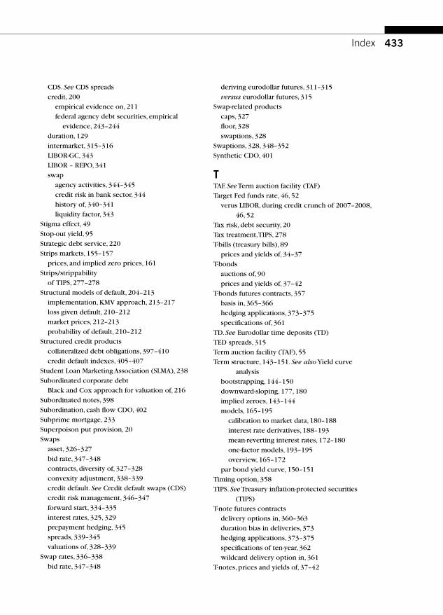
433 Index
CDS. See CDS spreads
credit , 200
empirical evidence on , 211
federal agency debt securities, empirical
evidence , 243 – 244
duration , 129
intermarket , 315 – 316
LIBOR-GC , 343
LIBOR – REPO , 341
swap
agency activities , 344 – 345
credit risk in bank sector , 344
history of , 340 – 341
liquidity factor , 343
Stigma effect , 49
Stop-out yield , 95
Strategic debt service , 220
Strips markets , 155 – 157
prices, and implied zero prices , 161
Strips/strippability
of TIPS , 277 – 278
Structural models of default , 204 – 213
implementation, KMV approach , 213 – 217
loss given default , 210 – 212
market prices , 212 – 213
probability of default , 210 – 212
Structured credit products
collateralized debt obligations , 397 – 410
credit default indexes , 405 – 407
Student Loan Marketing Association (SLMA) , 238
Subordinated corporate debt
Black and Cox approach for valuation of , 216
Subordinated notes , 398
Subordination, cash fl ow CDO , 402
Subprime mortgage , 233
Superpoison put provision , 20
Swaps
asset , 326 – 327
bid rate , 347 – 348
contracts, diversity of , 327 – 328
convexity adjustment , 338 – 339
credit default. See Credit default swaps (CDS)
credit risk management , 346 – 347
forward start , 334 – 335
interest rates , 325 , 329
prepayment hedging , 345
spreads , 339 – 345
valuations of , 328 – 339
Swap rates , 336 – 338
bid rate , 347 – 348
deriving eurodollar futures , 311 – 315
versus eurodollar futures , 315
Swap-related products
caps , 327
fl oor , 328
swaptions , 328
Swaptions , 328 , 348 – 352
Synthetic CDO , 401
T TAF. See Term auction facility (TAF)
Target Fed funds rate , 46 , 52
verus LIBOR, during credit crunch of 2007 – 2008 ,
46 , 52
Tax risk, debt security , 20
Tax treatment, TIPS , 278
T-bills (treasury bills) , 89
prices and yields of , 34 – 37
T-bonds
auctions of , 90
prices and yields of , 37 – 42
T-bonds futures contracts , 357
basis in , 365 – 366
hedging applications , 373 – 375
specifi cations of , 361
TD. See Eurodollar time deposits (TD)
TED spreads , 315
Term auction facility (TAF) , 55
Term structure , 143 – 151. See also Yield curve
analysis
bootstrapping , 144 – 150
downward-sloping , 177 , 180
implied zeroes , 143 – 144
models , 165 – 195
calibration to market data , 180 – 188
interest rate derivatives , 188 – 193
mean-reverting interest rates , 172 – 180
one-factor models , 193 – 195
overview , 165 – 172
par bond yield curve , 150 – 151
Timing option , 358
TIPS. See Treasury infl ation-protected securities
(TIPS)
T-note futures contracts
delivery options in , 360 – 363
duration bias in deliveries , 373
hedging applications , 373 – 375
specifi cations of ten-year , 362
wildcard delivery option in , 361
T-notes, prices and yields of , 37 – 42

434 Index
TRACE. See Trade Reporting and Compliance Engine
(TRACE)
Trade Reporting and Compliance Engine (TRACE) ,
64 –65
Trading characteristics, evidence on , 63–64
Trading strategies
curve fl attening trades , 118–119
curve steepening , 118–119
Trading volume
in secondary markets (2007) , 14
Tranche
CDX , 405–407
equity , 398 , 406
mezzanine , 398
senior , 399 , 407
Treasury auctions
announcement , 91–93
conducted by Fed , 53
cycles and fi nancing rates , 100–101
discriminatory , 97–98
mechanisms , 93–94
of money market instruments , 89
repo , 47–48 . See also Repo
theory and empirical evidence , 99–100
of TIPS , 90
of treasury bonds , 90
of treasury debt securities , 87–101. See also Debt
securities
of treasury notes , 89–90
uniform price , 94–97
when-issued trading and book building , 93
Treasury bills (T-bills) , 89
prices and yields of , 34–37
Treasury bonds. See T-bonds
Treasury debt securities
auctions , 87–101
auction cycles and fi nancing rates , 100–101
benchmark auctions , 87–91
conduct of , 91–98
steps in , 92
theory and empirical evidence , 99–100
Treasury futures contracts , 359–375
basis after carry/net basis , 369–370
cash-and-carry arbitrage , 366
conversion factor , 363–364
delivery options in treasury note futures contracts ,
360 –363
duration bias in deliveries , 373
fi nancing bonds , 367
hedging applications , 373–375
implied repo rate , 370–373. See also Repo
Treasury infl ation-protected securities (TIPS) ,
269 –290
auctions of , 90
break-even infl ation , 270 , 280–283
cash-fl ows , 283–288
structures , 278–280
in context of overall treasury debt , 271–272
design of , 275–278
choice of index , 275–276
indexation lag , 276–277
maturity composition , 277
strippability of , 277–278
tax treatment , 278
duration and nominal bonds , 289
investor’s perspective , 288–290
prices , 283–288
quotes , 270
risks of , 283–288
yields , 283–288
real/nominal , 280–283
Treasury markets , 58
Treasury notes (T-notes)
auctions of , 89–90
Treasury yields
Fannie Mae spreads over , 243–244
Tri-party repos , 85
in Europe and United States , 86
Trustee , 400
Twelve-year retirement, prepayment , 251
U Uniform price auctions , 94–97
United States
tri-party repos in , 86
Unsecured debt (debentures) , 7
Upward-sloping yield curve , 132
U.S. Treasury securities
Fed open market operations for , 47
V Valuation
of caps , 321–324
of OIS , 299–301
of swaps , 328–339
determine the forward rate , 330–332
using excel solver , 332
Value of equity
Black and Schole’s pricing model , 206–207
Variations around current yield, DV01 , 109

435 Index
Vasicek model , 175 – 177
Volatility
economic news announcements, and , 138 – 140
interest rates , 135 – 138
price-based vs yield-based , 138
W WAC. See Weighted average coupon (WAC)
Waterfalls, cash-fl ow CDO , 403
Weighted average coupon (WAC) , 246
When-issued (WI) market , 93
Wildcard delivery option , 361
WI market. See When-issued (WI) market
Winner’s curse , 99 – 100
Y Year-to-year cap, ARM , 231
Yield to maturity (YTM) , 126. See also Internal rate
of return (IRR)
defi ned , 207 – 208
excel solver for computing , 41
Yields
Fannie Mae spreads over treasury , 243 – 244
mortgage , 233 – 237
to settlement , 308 – 311
TIPS , 283 – 288
real/normal yields , 280 – 283
Yield curve analysis , 131 – 143. See also Term
structure
coupon effects , 140 – 143
economic news announcements, and volatility ,
138 – 140
models , 165 – 195
price-based vs yield-based volatility , 138
principal component analysis , 135 – 136
swaps , 191 – 192
vintage effects , 140 – 143
volatility, of interest rates , 135 – 138
vs duration , 140
Yield of debt security , 5
Yield to worst , 43
YTM. See Yield to maturity (YTM)
Z Zero coupon bonds. See also Implied zeroes
yield spreads for corporate , 211
Zero price extraction , 158 – 163