Fixed Effects Models Versus Mixed Effects Models for Clustered Data:Reviewing the Approaches, Disentangling the Differences,

and Making RecommendationsDaniel McNeish

Arizona State UniversityKen Kelley

University of Notre Dame

AbstractClustered data are common in many fields. Some prominent examples of clustering are employees clusteredwithin supervisors, students within classrooms, and clients within therapists. Many methods exist thatexplicitly consider the dependency introduced by a clustered data structure, but the multitude of availableoptions has resulted in rigid disciplinary preferences. For example, those working in the psychological,organizational behavior, medical, and educational fields generally prefer mixed effects models, whereas thoseworking in economics, behavioral finance, and strategic management generally prefer fixed effects models.However, increasingly interdisciplinary research has caused lines that separate the fields grounded inpsychology and those grounded in economics to blur, leading to researchers encountering unfamiliar statisticalmethods commonly found in other disciplines. Persistent discipline-specific preferences can be particularlyproblematic because (a) each approach has certain limitations that can restrict the types of research questionsthat can be appropriately addressed, and (b) analyses based on the statistical modeling decisions common inone discipline can be difficult to understand for researchers trained in alternative disciplines. This can impedecross-disciplinary collaboration and limit the ability of scientists to make appropriate use of research fromadjacent fields. This article discusses the differences between mixed effects and fixed effects models forclustered data, reviews each approach, and helps to identify when each approach is optimal. We then discussthe within–between specification, which blends advantageous properties of each framework into a singlemodel.

Translational AbstractEven though many different fields encounter data with similar structures, the preferred method for modelingsuch data can be vastly different from discipline to discipline. This is especially true in the case of clustereddata where in subsets of observations belong to the same higher order unit, as is common in organizationalscience, education, or longitudinal studies. To model such data, researchers trained in the economic traditionprimarily rely on fixed effects models, whereas researchers trained in the psychological tradition employmixed effects models. As the disciplinary lines between these economics and psychology continue to beblurred (e.g., in fields such as behavioral economics or strategic management), the disparity in approaches tostatistical modeling can prevent dissemination and proper interpretation of results. Additionally, each of thesestatistical methods has certain limitations that can prevent answering particular research questions, limiting thescope of hypotheses that can be tested. The goal of this article is to compare and contrast the fixed effect andmixed effect modeling frameworks to overview the general idea behind each and when employing eachmethod may be most advantageous. We also discuss ways in which aspects of both models can be blendedinto a single framework to maximally benefit from what each method can provide.

Keywords: fixed effect model, multilevel model, HLM, panel data, random coefficients model

Clustered data are ubiquitous in many contexts; classical cross-sectional examples include students nested within schools in edu-cational contexts, clients nested within therapists in clinical psy-

chology, patients nested within doctors in medicine, personsclustered within neighborhoods in epidemiology, employeesnested within firms in business, and hospitals within systems inhealth care (Hox, 2010; Raudenbush & Bryk, 2002; Snijders &Bosker, 2012). Clustering also occurs by repeated measures onmultiple units, often deemed longitudinal or panel data, in whichthe same information is tracked across time for the same units. Inthis context, the nesting structure is in terms of the multipleobservations being nested within a single entity (Bollen & Curran,2006; Greene, 2003; Rabe-Hesketh & Skrondal, 2008; Singer &Willett, 2003; Wooldridge, 2002). When data are cross-sectional,panel data, or a combination of the two, the nested structure of thedata must be accommodated in the analysis. A failure to do soviolates the independence assumption postulated by many popular

This article was published Online First June 4, 2018.Daniel McNeish, Department of Psychology, Arizona State University;

Ken Kelley, Department of Information Technology, Analytics, and Op-erations, and Department of Psychology, University of Notre Dame.

Correspondence concerning this article should be addressed to DanielMcNeish, Department of Psychology, Arizona State University, P.O. Box871104, Psychology Building, Tempe, AZ 85287, or to Ken Kelley,Department of Management–Analytics, University of Notre Dame, Men-doza College of Business, Notre Dame, IN 46556. E-mail: dmcneish@asu.edu or KKelley@ND.edu

Thi

sdo

cum

ent

isco

pyri

ghte

dby

the

Am

eric

anPs

ycho

logi

cal

Ass

ocia

tion

oron

eof

itsal

lied

publ

ishe

rs.

Thi

sar

ticle

isin

tend

edso

lely

for

the

pers

onal

use

ofth

ein

divi

dual

user

and

isno

tto

bedi

ssem

inat

edbr

oadl

y.

Psychological Methods© 2018 American Psychological Association 2019, Vol. 24, No. 1, 20–351082-989X/19/$12.00 http://dx.doi.org/10.1037/met0000182

20

models, which leads to biased standard error estimates (oftendownwardly biased) and improper statistical inferences (e.g., Li-ang & Zeger, 1986; Maas & Hox, 2005; Moulton, 1986, 1990;Raudenbush & Bryk, 2002; Wooldridge, 2003).

Fortunately, several methods exist to account for clustering sothat inferences made with clustered data are appropriate and yieldtest statistics that align with the theoretical properties (e.g., well-behaved Type I error rates and confidence interval coverage).There are strong disciplinary preferences by which clustered dataare modeled (McNeish, Stapleton, & Silverman, 2017). For exam-ple, a review performed by Bauer and Sterba (2011) found thatabout 94% of psychology studies between 2006 and 2011 ac-counted for clustering via mixed effects models (MEMs). Con-versely, a review by Petersen (2009) showed almost the exactopposite trend in econometrics—only 3% of studies reviewed usedMEMs. As noted in McNeish et al. (2017), MEMs are so fre-quently used in psychological research that it has, for all intentsand purposes, become synonymous with modeling clustered data.However, as noted by recent articles (Huang, 2016; McNeish &Stapleton, 2016), several alternative methods exist for modelingclustered data. In addition to classical approaches, such as within-subjects analysis of variance and multivariate analysis of variancefor modeling clustered data (e.g., Maxwell, Delaney, & Kelley,2018), more modern approaches have included the use of MEMs,which have become popular in psychology, or fixed effects models(FEMs), which have become popular in fields grounded in eco-nomics. Recent studies have contrasted the typical approach formodeling clustered data in psychology to methods common inbiostatistics, such as generalized estimating equations (McNeish etal., 2017), and survey methodology methods, such as Taylor serieslinearization (Huang, 2016). However, there has been less atten-tion paid to differences between MEMs that are widely adopted bypsychologists and FEMs that tend to be preferred by researchersworking in the econometric tradition. Given that there can beconsiderable disparities in training within psychology-adjacentfields (e.g., industrial-organizational psychology, managementstudies, education, and policy studies), researchers trained in onetradition may have difficulty comprehending the rationale behindthe analytic methods chosen by their colleagues within their ownfield but trained in another statistical tradition. This may result indifficulty interpreting statistical results in such fields, which cancause confusion and inhibit the pace of development as such fieldsmove forward.

This article reviews FEMs, which are popular in fields groundedin an econometrics tradition (A. Bell & Jones, 2015) but not wellknown in psychology. We provide comparisons between the FEMsand MEMs, making recommendations for when each should beused. Generally, FEMs account for a clustered data structure byincluding the cluster affiliation information directly into the modelas a predictor (i.e., a fixed effect) rather than treating cluster-specific quantities as random effects. In other words, FEMs areequivalent to adding categorical predictors to the model represent-ing the cluster variable (e.g., including an intercept for each personin a longitudinal model). Some researchers in fields related toeconomics have gone so far as to refer to the FEM framework asthe “gold standard” for modeling clustered data (Schurer & Yong,2012). In the political science literature, in which the econometrictradition has a strong presence, a recent article by A. Bell and

Jones (2015) tried to dissuade researchers from using FEMs,arguing that they are overused much in the same way that McNeishet al. (2017) argued that MEMs are overused in psychology.Clearly, some clarification and recommendations are needed tohelp clarify when each method is appropriate.

Despite the high praise for, and near ubiquity of, FEMs in theeconometrics and related literatures, psychological researchersseem largely indifferent with this modeling framework. As evi-dence for this claim, we searched two flagship empirical psychol-ogy journals for references to FEMs and MEMs: Journal ofPersonality and Social Psychology and Journal of Applied Psy-chology, during the publication years 2015 and 2016. In theJournal of Personality and Social Psychology, 0 of 247 studiescontain the phrase “fixed effects model” or “fixed-effects model.”When searching for “fixed effect” instead, we found three studies,but each of these referred to fixed factors in a fixed effectsANOVA context or a fixed effect in a MEM context. In theJournal of Applied Psychology, we found three studies from apossible 399 articles (0.8%) containing the phrase “fixed effectsmodel” or “fixed-effects model” as used in an FEM context. Themore relaxed search term “fixed effect” yielded two additionalstudies, but both of these additional used the phrase in the contextof ANOVA or MEMs. In a pair of searches performed in leadingeconomic journals, 33 of 79 articles (42%) published in the Quar-terly Journal of Economics during the same time period featuredFEMs, and 131 of 248 articles published in the Journal of Finan-cial Economics (53%) featured FEMs. There were also majordiscrepancies between statistical texts in their discussion of ana-lyzing clustered data. Texts commonly used in psychology, such asRaudenbush and Bryk (2002), Maxwell et al. (2018), and Hox(2010), do not feature any coverage of FEMs, whereas Snijdersand Bosker (2012) discuss FEMs only briefly (pp. 43–48). Con-versely, the Greene (2003)1 text on econometric analysis brieflydiscusses MEMs (pp. 293–295, 318–320), with additional discus-sion of the different estimation procedures (pp. 295–301).

This vast disconnect between fields with a psychological foun-dation and fields with an economic foundation begs the question,are psychology and related fields at a disadvantage by not consid-ering an entire modeling framework that is the principal approachto modeling clustered data in economics? Conversely, are econom-ics and related fields at a disadvantage by predominantly focusingtheir modeling efforts on FEMs? These questions have particularlystrong implications as disciplinary boundaries between business,psychology, and economics continue to be blurred.

To address the chasm between MEMs and FEMs, we provide anoverview of both the MEM and FEM frameworks to help readersunderstand alternative frameworks with which they may not befamiliar. We then discuss strengths and limitations of each modelfor types of analyses common in psychology and provide empiricalexamples. Particular emphasis is placed on discussion of the exo-geneity assumption of MEMs, whose tenability has led to differentmethods being preferred in different fields. We conclude with thewithin–between specification of a MEM, a method that incorpo-rates advantages of both FEMs and MEMs, especially with respectto treatment of the exogeneity assumption. We discuss how this

1 Page numbers refer to the fifth edition of this text.

Thi

sdo

cum

ent

isco

pyri

ghte

dby

the

Am

eric

anPs

ycho

logi

cal

Ass

ocia

tion

oron

eof

itsal

lied

publ

ishe

rs.

Thi

sar

ticle

isin

tend

edso

lely

for

the

pers

onal

use

ofth

ein

divi

dual

user

and

isno

tto

bedi

ssem

inat

edbr

oadl

y.

21FIXED VS. MIXED EFFECT MODELS

specification flexibly applies elements of both methods, makinganalyses stronger across both traditions.2

Overview of Mixed Effects Models

In MEMs, the clustered structure of the data is accounted for byincluding random effects in the model (Laird & Ware, 1982;Stiratelli, Laird, & Ware, 1984). Coefficients in MEMs representtwo possible types of effects: fixed effects or random effects. Fixedeffects are estimated to represent relations between predictors andthe outcome irrespective to which cluster observations belong,similar to a standard single-level multiple linear regression model(Raudenbush & Bryk, 2002). Random effects, on the other hand,capture how much the relation between the predictor and theoutcome differs from the fixed effect estimate for a specificcluster, essentially capturing the unique effect of the predictor inthe cluster of interest. Put another way, the effects within eachcluster form a distribution of effects in which the fixed effect is themean and the random effects are unique data points.

Mathematically, MEMs for continuous outcomes can be ex-pressed as

yj � Xj� � Zjuj � �j, (1)

where yj is an mj � 1 vector of responses for cluster j and mj is thenumber of units within cluster j, Xj is an mj � p design matrix forthe fixed predictors in cluster j (at either level) and p is the numberof predictors (including the intercept), � is a p � 1 vector ofregression coefficients, Zj is an mj � q design matrix for therandom effects of cluster j, uj is a q � 1 vector of random effectsfor cluster j, q is the number of random effects (where p � q),E(uj) � 0, Cov(uj) � G, G is q � q, �j is an mj � 1 vector ofresiduals of the observations in cluster j, E(�j) � 0, and Cov(�j) � R.Although there are several estimators that can be used to estimateMEMs, either maximum likelihood or restricted maximum likeli-hood are typically used (e.g., SAS Proc Mixed, SPSS, Stata, Rlme4). For more detail on the algorithms and methods typicallyemployed to estimate these models, see Goldstein (1986, 1989).For foundational information on restricted maximum likelihoodestimation, see Harville (1977) or Patterson and Thompson (1971).For a more general statistical overview of the mixed effects model,see Laird and Ware (1982). For a conceptual overview of thedifferences between maximum likelihood and restricted maximumlikelihood estimation, see McNeish (2017b).

Assumptions

Although MEMs permit rich models to be fit to clustered data,the inclusion of random effects in these models require that severalassumptions be made. An important assumption of MEMs is thatthe predictor variables included in the model do not covary witheither the residuals or the random effects (i.e., Cov[X, u] � Cov[X,r] � 0), which is commonly referred to as the exogeneity assump-tion (e.g., Gardiner et al., 2009). When the exogeneity assumptionis violated, the model is said to be endogenous, meaning that thereis an unmodeled relation that establishes nonzero covariance be-tween a predictor in the model and a random error term. That is,there are omitted confounders that threaten construct validity (e.g.,see Maxwell et al., 2018, for a review). If the exogeneity assump-tion is violated, then the coefficient estimates will contain notice-

able amounts of bias (Greene, 2003). We will return to this issuein subsequent sections, because differing disciplinary perspectiveson this assumption are a primary reason for preferring eitherMEMs or FEMs.

Other assumptions of MEMs include that (a) all relevant randomeffects have been included in the model, (b) the covariance struc-tures of the residuals and random effects have been properlyspecified, and (c) the residuals and the random effects followmultivariate normal distributions and do not covary across levels.Violating these assumptions can affect model selection as well asestimates and inferences made from the model. For more infor-mation on the ramifications of assumption violations, see Ebbes,Wedel, Böckenholt, and Steerneman (2005), Kim and Frees (2006,2007), McNeish et al. (2017), and Raudenbush and Bryk (2002,Chapter 9).

Hypothetical Example

Although matrix notation can help facilitate mathematical de-tails of MEMs, it is more common to see Raudenbush and Bryk(RB) notation in empirical applications. RB notation more clearlydisplays the location and relations between predictors and eluci-dates why these models are often referred to as hierarchical ormultilevel models. To demonstrate RB notation, consider an ex-ample in which work motivation (at Level 1, the employee level)and the quality of the company’s incentive program (at Level 2, thecompany level) predict employee productivity.3 This model wouldbe represented as

Productivityij � �0j � �1j Motivationij � rij (2a)

�0j � �00 � �01Incentivej � u0j (2b)

�1j � �10 � �11Incentivej, (2c)

where Productivityij is the productivity score for the ith employeein the jth company, �0j is the company-specific intercept for the jthcompany, �1j is the company-specific slope for motivation for thejth company, and rij is the residual for the ith person in the jthcompany.

2 Comparisons of FEMs and MEMs have appeared in other literaturesover the last decade (e.g., Clark & Linzer, 2015; Gardiner, Luo, & Roman,2009; Greene, 2003; Halaby, 2004; Yang & Land, 2008) but with littlerelevance to psychology. These previous treatments have focused on in-tersections of areas outside of psychology (healthcare and economics,economic sociology) and cover analyses that are germane to those areas butthat are not always common in psychology. The current article discussesthese models in contexts directly relevant to the study of psychologicalphenomenon.

3 The notation in Equation 1 does not differentiate at which level thepredictor exists. This can be seen much more clearly in RB notation. Level1 predictors are collected at the lowest level of the hierarchy (e.g., em-ployees if data are collected in companies, time-varying covariates if dataare collected longitudinally). These variables appear in the first equation inRB notation. Level 2 predictors are collected at the higher level of thehierarchy (e.g., company-level variables if data are collected on employeesclustered within companies; time-invariant predictors if data are collectedlongitudinally). Level 2 predictors can either be properties of the Level 2unit itself (e.g., school size) or an aggregation of the Level 1 units with theLevel 2 unit (e.g., average salary at a company). Although other methodsdo not formally adopt the level-specific designation of predictors, research-ers often use this terminology out of convenience.

Thi

sdo

cum

ent

isco

pyri

ghte

dby

the

Am

eric

anPs

ycho

logi

cal

Ass

ocia

tion

oron

eof

itsal

lied

publ

ishe

rs.

Thi

sar

ticle

isin

tend

edso

lely

for

the

pers

onal

use

ofth

ein

divi

dual

user

and

isno

tto

bedi

ssem

inat

edbr

oadl

y.

22 MCNEISH AND KELLEY

Equation 2a then allows researchers to model the company-specific intercept (�0j; i.e., the Level 1 coefficients in Equation 2aare the dependent variables in Equations 2b and 2c). In Equation2b, �00 is the overall intercept for productivity across all compa-nies, �01 is a regression coefficient that captures how much theintercept of productivity is expected to change for a one-unitchange in incentive for company j, and u0j is a random effect forthe jth company that captures how much the intercept for the jthcompany differs from the overall intercept �00 after accounting forincentive. The company-specific intercepts �0j follow a normaldistribution that is centered on �00 � �01Incentivej, with a variancedenoted by �00 in this notation. If u0j is not included in Equation2b, then this implies that �00, the variance of the intercepts betweendifferent clusters, is equal to zero. Equation 2c contains similarinformation as Equation 2b except that the outcome is now thecompany-specific slope (�1j) rather than the company-specificintercept. In Equation 2c, the absence of a random effect formotivation means that, controlling for the incentive, the effect ofmotivation on productivity does not vary between companies. Thethree separate equations can be combined into one single equationsuch that

Productivityij � �00 � �01Incentivej

� (�10 � �11Incentivej) � Motivationij � u0j � rij. (3)

Note that Equation 3 contains a “mix” of the fixed effect �parameters as well as the random effect u parameter, giving rise tothe “mixed effect model” name.

In general, MEMs are a flexible method that allows researchersmuch freedom in building models that test their research questionsand theories. However, researchers pay for this flexibility withassumptions.

Overview of Fixed Effects Models

As noted in Gelman and Hill (2006, p. 245) and Gardiner et al.(2009), the term “fixed effect” has several, nonoverlapping defi-nitions when used in various branches of statistics. When psychol-ogists hear or see “fixed effects,” they tend to think of (a) param-eters in MEMs that represent the association between a Level 1predictor and the outcome across all clusters, or (b) levels of oneor more factors (e.g., control group, Treatment A, Treatment B)that are purposely chosen in the context of analysis of variance.

In the econometric tradition, “fixed effects” does not refer to aparticular component of a model for clustered data or a type ofresearch design. Rather, “fixed effects” refers to an entire model-ing framework (Allison, 2009). Similar to MEMs, FEMs explicitlymodel the clustered structure of the data. However, FEMs do notuse random effects or random coefficients (i.e., the u parameter inEquation 2 and 3). Instead, cluster affiliation dummy variables areincluded directly in the model as predictor variables. A regressioncoefficient is then estimated for each cluster affiliation variable toyield cluster-specific estimates, much in the same way that eachcluster has a unique random intercept estimate in MEMs (Gardineret al., 2009). To make another connection, the FEM can be seen asan ANCOVA in which the cluster affiliation is a categorical factorpredicting the outcome. All variability at Level 2 is explained inthe FEM because the cluster affiliation variables are treated aspredictors (unlike MEMs, in which Level 2 variability is a parti-

tioned component of the residual variance). Unlike traditionalANCOVA, the focus of the FEM is on the covariates, with thecategorical cluster factor serving as a control variable to accountfor the data structure.

Such a specification has noticeable ramifications for how vari-ability at Level 2 is accounted for, which can be viewed as anadvantage or disadvantage depending on the research question athand. Though we will discuss this issue in much more detail insubsequent sections, the general consequence of the FEM is thatthe cluster affiliation variables account for all of the variability atLevel 2. This means that researchers need not be concerned withincluding Level 2 predictors in the model, because variance attrib-utable to all Level 2 variables (whether available in the data or not)is consumed by the cluster affiliation variables. As a result, allLevel 1 coefficients are conditional on all possible Level 2 effects.As a cost of such a strategy, researchers lose the ability to estimatecoefficients for any individual Level 2 predictor in the model—once the cluster affiliation variables are included in the model,only coefficients for Level 1 predictors can be estimated.

MEMs assume that random effects are drawn from a particulardistribution (often a normal distribution); however, FEMs do notassume that clusters are a random sample from the possible pop-ulation of clusters. This represents one reason why FEMs tend tobe popular in economics research—clustering units are frequentlyselected for a specific purpose (e.g., European countries, chiefexecutive officers from Fortune 100 companies, top-rated univer-sities) instead of being randomly selected.

In FEMs, the creation of cluster-specific affiliation variables canbe done with two different dummy-coding methods. The firstmethod of coding, which we will refer to as absolute coding, is toinclude as many cluster affiliation variables as there are clustersand to remove the intercept to prevent overparameterization of themodel. In this case, estimates for the cluster affiliation variablesrepresent the intercept value for each specific cluster, similar tohow each cluster receives a cluster-specific intercept estimate inMEMs. Another method of coding, which we refer to as referencecoding, is to retain the intercept estimate in the model and leaveone of the cluster affiliation variables out as a reference cluster.Cluster affiliation variable estimates with this method represent thedifference in the intercept between a specific cluster and thereference cluster whose cluster affiliation variable was omittedform the model. Thus, the first method gives the cluster affiliationestimates an absolute interpretation, whereas the second methodgives a relative interpretation.

Notationally, using an absolute coding scheme, the FEM can bewritten as

yj � Xj� � Cj� � rj, (4)

where yj is an mj � 1 vector of responses for the jth cluster,4 Xj isan mj � p design matrix of substantive predictors, � is a p � 1vector of substantive regression coefficients, Cj is an N � J matrixof cluster affiliation dummy codes, � is a J � 1 vector of

4 Readers may note that the FEM is a single-level model, but we definethe model using j subscripts to denote the cluster. Though not required, weuse this model notation because it elucidates the role of the cluster affili-ation dummy variables and the associated coefficients. Otherwise, thisinformation would be appended to the end of the � matrix, where itsfunction may be less clear.

Thi

sdo

cum

ent

isco

pyri

ghte

dby

the

Am

eric

anPs

ycho

logi

cal

Ass

ocia

tion

oron

eof

itsal

lied

publ

ishe

rs.

Thi

sar

ticle

isin

tend

edso

lely

for

the

pers

onal

use

ofth

ein

divi

dual

user

and

isno

tto

bedi

ssem

inat

edbr

oadl

y.

23FIXED VS. MIXED EFFECT MODELS

cluster-specific intercepts, and rj is an mj � 1 vector of residualsthat is traditionally assumed to be distributed N (0, �2I). Becausethe cluster affiliation dummy variables account for all cluster-levelvariance, the FEM residual variance is equivalent to the Level 1residual variance in MEMs, not the total residual variance acrossall levels. Because there are no random effects in the model,5

FEMs with continuous outcomes are often estimated with ordinaryleast squares (OLS; the same as a single-level multiple linearregression model). The form of the model presented in Equation 4assumes that coefficients are equal across clusters. As will bediscussed later, this can be relaxed.

Assumptions

A primary benefit of the FEM framework is that there are farfewer assumptions compared with MEMs. In FEMs, the modelonly needs to be properly specified with respect to Level 16

predictors (time-varying predictors in panel data) for the parameterestimates and standard errors to have desirable statistical proper-ties: The cluster affiliation dummy variables handle all possibleLevel 2 predictors (time-invariant predictors in panel data) regard-less of whether the variable was collected in the data or not. Level1 predictors must have variability within clusters because FEMsonly explicitly model within-group variation (all variables withoutwithin-group variance are accounted for by the cluster affiliationdummy variables). This means that effects for Level 2 predictorscannot be directly estimated within a FEM (Baltagi, 2013; Hsiao,2003; Kim & Frees, 2006), although they will be accounted for inthe model via the cluster affiliation dummy variables (i.e., othereffects are conditional on the Level 2 predictors, but effects ofspecific Level 2 variables are not estimable). If an FEM model isestimated with OLS, then it is conventional to assume that theresiduals are distributed N (0, �2I). This assumption may bereasonable with cross-sectional clustering but could be violatedwith panel data because of the presence of autocorrelation (A. Bell& Jones, 2015), meaning that the residuals at different time pointsare not independent of one another. However, other estimationmethods like generalized least squares or maximum likelihood canaccount for this dependence with different types of residual struc-tures (e.g., compound symmetry, Toeplitz). Unlike MEMs, FEMsdo not assume that clusters are sampled randomly.

Hypothetical Example

To see how FEMs differ from MEMs, consider the examplefrom the previous section in which employee productivity is pre-dicted by work motivation and the quality of the company’sincentive program. If there are five companies in the data, the FEMwould be written out completely as

Productivityij � �1Motivationij � �2(Motivationij � Incentivej)

� �1Company1 � �2Company2 � �3Company3

� �4Company4 � �5Company5 � rij, (5)

where �1 captures the relation between motivation and productiv-ity, �2 captures how the effect of motivation changes depending onthe values of incentive (i.e., the interaction of the two), and the parameters represent the company-specific intercepts (we use theabsolute coding here). Notice that the incentive predictor does not

explicitly appear in the model as a separate term (although it doesappear as part of an interaction) because the main effect of incen-tive is included in the variance accounted for by the companyvariables. The tests for motivation and the Motivation � Incentiveinteraction therefore control for incentive even though it is nolonger possible to estimate the specific effect of incentive, becausethis variable is perfectly collinear with the company variables. Thisis an important distinction in FEMs—the cluster affiliation vari-ables include all the measured and unmeasured variables at Level2 even though the specific effects of Level 2 predictors are unob-tainable. That is, all effects in the model are conditional onincentive (and all other Level 2 variables), but the main effect forincentive specifically is inestimable. The company variables sub-sume all Level 2 variables and explain all the variance at Level 2;therefore, there is no unique variance left for any single Level 2variable to explain because any variance explained any Level 2variables will necessarily overlap completely with variance ex-plained by the company variables. The Motivation � Incentiveinteraction term is permissible even though it involves a Level 2variable because there is still within-cluster variation once themultiplicative term is created. Table 1 shows how parameters fromEquation 2 map onto parameters in Equation 5.

De-Meaning

The previous FEM description is commonly referred to as theleast square dummy variable (LSDV) fixed effects model. There isanother alternative specification that may be used to achieve thesame goal without needing to create dummy variables, which canbe useful when there are many clusters and estimation would becomputationally burdensome with many dummy variables (e.g., inbig data; Allison, 2009).7 This alternative approach is referred toas de-meaning, in which the cluster means are subtracted from theobserved values for all variables. The de-meaned version of Equa-tion 5 without the Motivation � Incentive cross-level interactionwould be

�Productivityij Productivity�j) � �1(Motivationij Motivation�j)

� (rij r�j). (6)

To demonstrate how de-meaning works, consider Equation 5 asa random intercepts MEM such that

Productivityij � �1Motivationij � u0j � rij. (7)

5 Technically, FEMs do have a random component in the model becausethe residuals are random effects and are assumed to be randomly drawnfrom a particular distribution. In this article, we reserve use of “randomeffects” for random effects at Level 2 and refer to what are technicallyLevel 1 random effects as “residuals.”

6 Although we talk about “levels” in FEMs, note that FEMs do notconsider different levels of analysis as in MEMs. The FEM model does notdifferentiate between Level 1 or Level 2 variables. The FEM is an inher-ently single-level regression model that uses clever coding to manipulatethe single-level framework into estimating coefficients from clustered data.We use “Level 1” and “Level 2” to facilitate the discussion about param-eters that are similarly estimated by MEMs and FEMs. In the FEMframework, Level 1 means that the variable has variability within clusters,whereas Level 2 means that that variable has no variability within a cluster.

7 Such big data situations will likely become more common in psychol-ogy and related fields due to the instrumented world in which we now liveand such methods can measure various aspects of behavior (e.g., Adjerid &Kelley, 2018).

Thi

sdo

cum

ent

isco

pyri

ghte

dby

the

Am

eric

anPs

ycho

logi

cal

Ass

ocia

tion

oron

eof

itsal

lied

publ

ishe

rs.

Thi

sar

ticle

isin

tend

edso

lely

for

the

pers

onal

use

ofth

ein

divi

dual

user

and

isno

tto

bedi

ssem

inat

edbr

oadl

y.

24 MCNEISH AND KELLEY

If Equation 7 were de-meaned (i.e., means are subtracted so thatthe variables are in terms of deviations from the mean), anyvariable with no variation within clusters (i.e., Level 2 predictorsand random effects) will be reduced to a constant value of zero andwill therefore drop out of the model because the cluster mean andthe observed values will necessarily be identical:

�Productivityij Productivity�j)

� �1(Motivationij Motivation�j) � (u0j u�0j) � (rij r�j)

� �1(Motivationij Motivation�j) � (rij r�j). (8)

Equation 6 and Equation 8 are the same and are also equivalentto Equation 5 without the Motivation � Incentive interaction term.However, there is a difference in implementation. Using the LSDVFEM, software will use the correct degrees of freedom for thestandard error calculation, because the cluster affiliation dummyvariables are directly included in the model and consume onedegree of freedom each, as with any categorical predictor. In thede-meaned approach, degrees of freedom will not be computedproperly because the subtraction of the means occurs as a datapreprocessing step that precedes the estimation of the model. As aresult, the p values and inferential tests will not be correct and mustbe adjusted to reflect the implicit inclusion of the cluster means inthe model (Judge, Griffiths, Hill, & Lee, 1985).

Comparing MEMs and FEMs

MEMs and FEMs each offer defensible ways to model clustereddata and have the same general goal. However, there are consid-erable differences with regard to the type of analytic scenarios inwhich each can be optimally applied, or even applied at all.Differences between these two approaches across a range of sce-narios are summarized in Table 2. In the subsequent sections, weprovide additional discussion to highlight the more salient differ-ences between the methods.

Sample Size

In many disciplines, the number of clusters in data sets tends tobe small due to practical concerns, such as financial limitations,

the use of extant data sets, or difficulties in recruiting largenumbers of participants (Dedrick et al., 2009; McNeish & Staple-ton, 2016). MEMs applied to data with fewer than 30 clusters havebeen shown to be at risk for downwardly biased estimates of thevariance component and regression coefficient standard error es-timates (e.g., B. Bell, Morgan, Schoeneberger, Kromrey, & Ferron,2014; Maas & Hox, 2005). Several remedies have been proposed,including the Kenward-Roger correction (Kenward & Roger,1997), Bayesian Markov Chain Monte Carlo (MCMC) estimation(Hox, van de Schoot, & Matthijsse, 2012), and Monte Carloresampling methods (Bates, 2010). These methods are generallyserviceable in practice although they are not without their faults(e.g., Ferron, Bell, Hess, Rendina-Gobioff, & Hibbard, 2009;McNeish, 2016, 2017b).

Because FEMs are routinely estimated with OLS, they tend tobe much less susceptible to bias when data have very few clusters,because standard errors have a closed form and there is no need toestimate variance components. For example, for cross-sectionalclustering and fewer than 15 clusters, McNeish and Stapleton(2016) found that FEMs performed the best overall with respect tominimizing bias, controlling Type I error rates, and maximizingpower from among 12 competing small sample methods, includingMCMC MEMs with the half-Cauchy prior recommended for smallsamples by Gelman (2006).

As noted previously, coefficient estimates of Level 2 predictorscannot be obtained from FEMs. This may lead some researchers toacknowledge the superior small sample performance, but note thatFEMs ultimately do not estimate all the quantities that are often ofinterest in many contexts. Although true, note that these Level 2coefficients are typically estimated rather poorly with fewer than20 clusters (Baldwin & Fellingham, 2013; Hox et al., 2012; Steg-mueller, 2013), so researchers should carefully consider the im-portance of Level 2 coefficients in such cases. Prioritizing theestimation of these Level 2 coefficients could lead to biasedestimates throughout a MEM, whereas a FEM would limit thecoefficient estimates to Level 1 coefficients. However, FEMswould safeguard against bias for the estimates the model doesyield (i.e., Level 1 coefficients) while controlling for measured andunmeasured Level 2 effects, provided that FEM assumptions aremet.

Cross-Level Interactions

Cross-level interactions refer to an interaction of two variablesin which one variable is at Level 1 (e.g., the employee level) andthe other is at Level 2 (e.g., the company level).8 Cross-levelinteractions can be tested using either the FEM or MEM frame-work, with examples being presented in Equation 2 and Equation5. In Equation 2, the cross-level interaction for a MEM is presentby modeling the coefficient of a Level 1 predictor as a function ofa Level 2 predictor (the �11 specifically represents this cross-levelinteraction effect). In the FEM model in Equation 5, the samecross-level interaction effect is captured by the �2 parameter.

8 Although we talk about “levels” in FEMs, note that FEMs do notconsider different levels of analysis as in MEMs. The FEM model does notdifferentiate between Level 1 or Level 2 variables. The FEM is an inher-ently single-level regression model that uses clever coding to manipulatethe single-level framework into estimating coefficients from clustered data.

Table 1Comparison of MEM and FEM Model Parameters

From MEM To FEM From FEM To MEM

�00 Weighted average of 1 to 5 �1 �10

�01 None, included in 1 to 5 �2 �11

�10 �1 1 u01

�11 �2 2 u02

u0j j� 3 u03

rij rij 4 u04

5 u05

rij rij

Note. MEM � mixed effects model; FEM � fixed effects model.� and u are conceptually related but are not the same. j are fixed effects,whereas uj are random effects. Depending on how the FEM is specified, j

is either the complete intercept for cluster j or the difference between theintercept of cluster j and a reference cluster. In MEM, uj are the deviationsfrom the overall mean and are defined to have a mean of 0. Even if all otheraspects of the model are identical, the uj and j estimates will differbecause uj will be shrunken via empirical Bayes estimation.

Thi

sdo

cum

ent

isco

pyri

ghte

dby

the

Am

eric

anPs

ycho

logi

cal

Ass

ocia

tion

oron

eof

itsal

lied

publ

ishe

rs.

Thi

sar

ticle

isin

tend

edso

lely

for

the

pers

onal

use

ofth

ein

divi

dual

user

and

isno

tto

bedi

ssem

inat

edbr

oadl

y.

25FIXED VS. MIXED EFFECT MODELS

Although FEMs do not allow for Level 2 predictors to beincluded in the model, cross-level interactions can be assessed withFEMs, because interactions of variables collected at differentlevels (e.g., employee and supervisor; client and therapist, studentand teacher) will differ for each Level 1 unit and will therefore notbe perfectly collinear with the cluster affiliation variables (i.e.,there is within-cluster variation). To include these predictors in aFEM, similar to MEM, a product term is created and included inthe model. Even though the Level 2 predictor cannot be includedin the model, the Level 2 predictor main effect is still controlled forby the cluster affiliation dummy variables because these variablesaccount for all variance attributable to measured and unmeasuredLevel 2 variables (Allison, 2009). Interactions of two Level 1variables are also permissible in FEMs, but interaction effects oftwo Level 2 variables are not possible in FEMs because there willbe no within-cluster variation.

Cluster-Varying Effects

A common research question is whether Level 1 effects vary indifferent clusters. For example, in an organizational setting, aresearcher may want to determine if the effect of motivation onproductivity is the same across supervisors. In MEMs, this isstraightforward to test—one only needs to include a random slopefor the Level 1 variable of interest (motivation, in this hypotheticalexample). If the associated random effect has a large variance

relative to the magnitude of the coefficient, then it can be con-cluded that the effect differs depending to which cluster an em-ployee belongs. Otherwise, the effect can be declared constantacross clusters and the random effect removed. Using the hypo-thetical example from Equation 2, the effect of motivation onproductivity can vary by clusters by adding a single random effect(u1j) into the model, such that

Productivityij � �0j � �1jMotivationij � rij (9a)

�0j � �00 � �01Incentivej � u0j (9b)

�1j � �10 � �11Incentivej � u1j (9c)

Similar to the interpretation of the random intercept (u0j) above,u1j allows the company-specific slope �0j to change for eachcompany beyond the change predicted by incentive. The u1j termcaptures the difference in the effect of motivation from the overallslope �10 for the jth cluster, conditional on incentive.

In FEMs, cluster-varying effects are possible but are moredifficult to specify and interpret. As discussed so far, clusteraffiliation coefficients in FEMs are similar to a random interceptsMEMs such that each cluster receives a unique intercept estimate.However, the Level 1 coefficients in FEMs do not vary acrossclusters as described so far, which would be equivalent to a MEMwithout random slopes. If cluster-varying effects are desired, thiscan be accomplished by including an interaction term between the

Table 2Comparison of the Types of Modeling Questions That Can Be Assessed With MEMs and FEMs

Modeling problem MEM FEM

Accommodation of clustering Random effects must be explicitly modeled bythe user. The covariance matrix of therandom effects also must be explicitlymodeled.

Cluster affiliation dummy variables are includeddirectly in the model.

Common estimation method (Restricted) Maximum likelihood Ordinary least squaresPredictors at Level 2 Allowed and coefficients are directly

estimated. Proper specification is required,meaning that no relevant variables areomitted.

Generally not estimable (although there are proposedmethods that claim to be able to provide estimatesunder particular circumstances). Omitted Level 2variable bias is not a concern.

Omitted variable bias A concern at all levels Only a concern at Level 1Accommodation of variability at

Level 2Predictor variables and random effects Cluster affiliation dummy variables

Coefficient interpretation Coefficients at either level are interpretedconditional on the variables explicitlyincluded in the model.

Level 1 coefficients are conditional on all Level 2variables (measured and unmeasured) beingaccounted for.

Level 2 sample size requirement 30 is the general recommendation; can bereduced (to about 10) if correctiveprocedures are used

Viable with very small Level 2 sample sizes

Cluster-varying slopes Easily modeled with random effects Must use interaction terms with cluster affiliationvariables

Supports impure hierarchies Yes NoEfficiency More efficient (smaller standard errors) but

more likely to be biased if assumptions areviolated or if the model is misspecified

Less efficient but less likely to produce biasedestimates because there are fewer assumptions andfewer locations where misspecifications can occur

Mediation possible Yes Only if all variables are at Level 1Analysis of contextual effects Yes NoCross-level interactions Yes YesExtendable to three-level hierarchies

(or more) Yes Not with a purely FEMAssumption about sampling of

clustersClusters are randomly sampled and

representative of the populationClusters need not be randomly sampled

Note. MEM � mixed effects model; FEM � fixed effects model.

Thi

sdo

cum

ent

isco

pyri

ghte

dby

the

Am

eric

anPs

ycho

logi

cal

Ass

ocia

tion

oron

eof

itsal

lied

publ

ishe

rs.

Thi

sar

ticle

isin

tend

edso

lely

for

the

pers

onal

use

ofth

ein

divi

dual

user

and

isno

tto

bedi

ssem

inat

edbr

oadl

y.

26 MCNEISH AND KELLEY

cluster affiliation variables and the Level 1 predictor into themodel. In this way, the Level 1 predictor will be estimated to havea unique effect in each cluster.

To make this model more explicit, recall the hypothetical ex-ample of modeling productivity as a function of motivation andincentive. In Equation 5, the model posits that the effect of moti-vation is constant across all companies, conditional on the othereffects that are in the model. If a researcher wanted to modelunique effects for motivation in each company, the main effect forMotivation would be removed and Motivation � Company inter-actions would be included, such that

Productivityij � �1(Motivationij � Company1)

� �2(Motivationij � Company2)

� �3(Motivationij � Company3)

� �4(Motivationij � Company4)

� �5(Motivationij � Company5) � �1Company1

� �2Company2 � �3Company3 � �4Company4

� �5Company5 � rij (10)

Coefficients �1 through �5 now represent the effect of motiva-tion on productivity for each respective cluster, similar to randomeffects in a MEM. There are also alternative ways in which thiscould be coded, such as leaving the main effect of motivation inthe model but including J – 1 interaction terms (i.e., referencecoding). The coefficients of these interaction terms would thenrepresent the difference in the effect of motivation on produc-tivity from the effect of motivation in the reference cluster. As canbe seen from Equation 10, if there are many clusters in the model,estimation of the model with this approach can quickly becomeburdensome due to the large number of parameters.

Although this type of specification can achieve the goal ofmodeling a cluster-varying effect within the FEM framework, suchan approach does have disadvantages. One disadvantage is thateach cluster affiliation by Level 1 predictor interaction coefficientwill consume a degree of freedom, meaning that researchers maynot have enough degrees of freedom to estimate multiple cluster-varying effects or even a single cluster-varying effect if there aremany predictors in the model. Another disadvantage is that, unlikeMEMs, which estimate a variance component for the randomslopes, which can inferentially tested (although specialized 50:50mixture chi-square tests are usually needed for this test; see Stram& Lee, 1994), FEMs have less intuitive methods to infer whethera cluster-varying effect is needed in the model. If reference codingis used such that the interaction terms are compared with a refer-ence cluster, a multiparameter test for the interaction term (e.g.,omnibus F test, Wald multiparameter Type III test) may providehelpful inferential information. With absolute coding, such a mul-tiparameter test would likely be of little use, because it would betesting whether the cluster slopes are collectively equal to zerorather than testing if they are different from each other (withreference coding, these two questions are synonymous). The vari-ance of the cluster affiliation effects can also be calculated bysaving all of the estimates and running descriptive statistics, al-though this will not be equal to a MEM variance componentestimate because it will not account for aspects such as unequalcluster sizes or differential reliability in each cluster.

Mediation

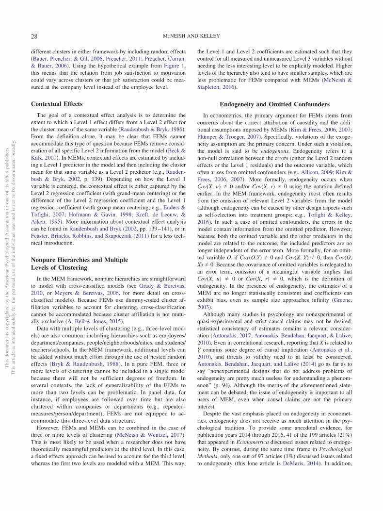
Using our running example, suppose that a researcher’s interestis, again, the effect of motivation on productivity; however, now itis of interest to test whether the effect of job satisfaction onproductivity is mediated by motivation. Mediation analysis is oneof the most important methods for explaining causal pathways.Mediation analyses with clustered data can also be modeled ineither the MEM or FEM framework as well as other frameworks(e.g., structural equation modeling, linear regression). A path di-agram for this type of mediation model in the FEM framework isdisplayed in Figure 1. FEMs can only model mediation if all thevariables are at Level 1. This would correspond to the so-called1–1–1 mediation model, in which all variables of interest are at thelowest level of the hierarchy but are clustered within higher levelunits. Level 2 variables cannot be included in a FEM mediationmodel because they are collinear with the cluster affiliation vari-ables (Hayes, 2013).

In Figure 1, the cluster affiliation dummy variables are predic-tors of both the mediator (motivation) and the outcome (produc-tivity) because both serve as dependent variables in the system.The independent variable (job satisfaction) is an exogenous vari-able in the model (in that no arrows point to job satisfaction) andtherefore need not be regressed on the cluster affiliation dummyvariables. As noted in Hayes (2013), the FEM specification assumesthat the effects of the coefficients do not vary across clusters. It ispossible to create Cluster Affiliation � Predictor Variable interactionterms, as was discussed in the previous section, to overcome this,although the interpretation of the model would be similarly difficult.The intercepts of motivation and productivity must also be con-strained to zero if using absolute coding in order to avoid overparam-eterizing the model. Alternatively, the intercepts could be retained ifreference coding were used.

If relations beyond what can be tested in a 1–1–1 model are ofinterest, then one can use either a MEM framework (Krull &MacKinnon, 1999) or the closely related multilevel structuralequation modeling (ML-SEM) framework (Kenny, Korchmaros,& Bolger, 2003; Preacher, Zyphur, & Zhang, 2010; Zhang, Zy-phur, & Preacher, 2009). These frameworks allow researchers totest mediation involving Level 2 predictors, with the ML-SEMallowing for the most general models (Preacher et al., 2010).Importantly, it is easy to allow coefficients to differ across the

Figure 1. Path diagram for 1–1–1 mediation models using a fixed effectsapproach. The cluster affiliation variables are depicted as a single box—inthe actual path diagram each cluster affiliation variable would be repre-sented by its own box. a, b, and c � mediation paths; Job Sat. � JobSatisfaction; Mot. � Motivation; Prod. � Productivity.

Thi

sdo

cum

ent

isco

pyri

ghte

dby

the

Am

eric

anPs

ycho

logi

cal

Ass

ocia

tion

oron

eof

itsal

lied

publ

ishe

rs.

Thi

sar

ticle

isin

tend

edso

lely

for

the

pers

onal

use

ofth

ein

divi

dual

user

and

isno

tto

bedi

ssem

inat

edbr

oadl

y.

27FIXED VS. MIXED EFFECT MODELS

different clusters in either framework by including random effects(Bauer, Preacher, & Gil, 2006; Preacher, 2011; Preacher, Curran,& Bauer, 2006). Using the hypothetical example from Figure 1,this means that the relation from job satisfaction to motivationcould vary across clusters or that job satisfaction could be mea-sured at the company level instead of the employee level.

Contextual Effects

The goal of a contextual effect analysis is to determine theextent to which a Level 1 effect differs from a Level 2 effect forthe cluster mean of the same variable (Raudenbush & Bryk, 1986).From the definition alone, it may be clear that FEMs cannotaccommodate this type of question because FEMs remove consid-eration of all specific Level 2 information from the model (Beck &Katz, 2001). In MEMs, contextual effects are estimated by includ-ing a Level 1 predictor in the model and then including the clustermean for that same variable as a Level 2 predictor (e.g., Rauden-bush & Bryk, 2002, p. 139). Depending on how the Level 1variable is centered, the contextual effect is either captured by theLevel 2 regression coefficient (with grand-mean centering) or thedifference of the Level 2 regression coefficient and the Level 1regression coefficient (with group-mean centering; e.g., Enders &Tofighi, 2007; Hofmann & Gavin, 1998; Kreft, de Leeuw, &Aiken, 1995). More information about contextual effect analysiscan be found in Raudenbush and Bryk (2002, pp. 139–141), or inFeaster, Brincks, Robbins, and Szapocznik (2011) for a less tech-nical introduction.

Nonpure Hierarchies and MultipleLevels of Clustering

In the MEM framework, nonpure hierarchies are straightforwardto model with cross-classified models (see Grady & Beretvas,2010, or Meyers & Beretvas, 2006, for more detail on cross-classified models). Because FEMs use dummy-coded cluster af-filiation variables to account for clustering, cross-classificationcannot be accommodated because cluster affiliation is not mutu-ally exclusive (A. Bell & Jones, 2015).

Data with multiple levels of clustering (e.g., three-level mod-els) are also common, including hierarchies such as employees/department/companies, people/neighborhoods/cities, and students/teachers/schools. In the MEM framework, additional levels canbe added without much effort through the use of nested randomeffects (Bryk & Raudenbush, 1988). In a pure FEM, three ormore levels of clustering cannot be included in a single modelbecause there will not be sufficient degrees of freedom. Inseveral contexts, the lack of generalizability of the FEMs tomore than two levels can be problematic. In panel data, forinstance, if employees are followed over time but are alsoclustered within companies or departments (e.g., repeated-measures/person/department), FEMs are not equipped to ac-commodate this three-level data structure.

However, FEMs and MEMs can be combined in the case ofthree or more levels of clustering (McNeish & Wentzel, 2017).This is most likely to be used when a researcher does not havetheoretically meaningful predictors at the third level. In this case,a fixed effects approach can be used to account for the third level,whereas the first two levels are modeled with a MEM. This way,

the Level 1 and Level 2 coefficients are estimated such that theycontrol for all measured and unmeasured Level 3 variables withoutneeding the less interesting level to be explicitly modeled. Higherlevels of the hierarchy also tend to have smaller samples, which areless problematic for FEMs compared with MEMs (McNeish &Stapleton, 2016).

Endogeneity and Omitted Confounders

In econometrics, the primary argument for FEMs stems fromconcerns about the correct attribution of causality and the addi-tional assumptions imposed by MEMs (Kim & Frees, 2006, 2007;Plümper & Troeger, 2007). Specifically, violations of the exoge-neity assumption are the primary concern. Under such a violation,the model is said to be endogenous. Endogeneity refers to anon-null correlation between the errors (either the Level 2 randomeffects or the Level 1 residuals) and the outcome variable, whichoften arises from omitted confounders (e.g., Allison, 2009; Kim &Frees, 2006, 2007). More formally, endogeneity occurs whenCov(X, u) 0 and/or Cov(X, r) 0 using the notation definedearlier. In the MEM framework, endogeneity most often resultsfrom the omission of relevant Level 2 variables from the model(although endogeneity can be caused by other design aspects suchas self-selection into treatment groups; e.g., Tofighi & Kelley,2016). In such a case of omitted confounders, the errors in themodel contain information from the omitted predictor. However,because both the omitted variable and the other predictors in themodel are related to the outcome, the included predictors are nolonger independent of the error term. More formally, for an omit-ted variable O, if Cov(O,Y) 0 and Cov(X, Y) 0, then Cov(O,X) 0. Because the covariance of omitted variables is relegated toan error term, omission of a meaningful variable implies thatCov(X, u) 0 or Cov(X, r) 0, which is the definition ofendogeneity. In the presence of endogeneity, the estimates of aMEM are no longer statistically consistent and coefficients canexhibit bias, even as sample size approaches infinity (Greene,2003).

Although many studies in psychology are nonexperimental orquasi-experimental and strict causal claims may not be desired,statistical consistency of estimates remains a relevant consider-ation (Antonakis, 2017; Antonakis, Bendahan, Jacquart, & Lalive,2010). Even in correlational research, reporting that X is related toY contains some degree of causal implication (Antonakis et al.,2010), and threats to validity need to at least be considered.Antonakis, Bendahan, Jacquart, and Lalive (2014) go as far as tosay “nonexperimental designs that do not address problems ofendogeneity are pretty much useless for understanding a phenom-enon” (p. 94). Although the merits of the aforementioned state-ment can be debated, the issue of endogeneity is important to allusers of MEM, even when causal claims are not the primaryinterest.

Despite the vast emphasis placed on endogeneity in economet-rics, endogeneity does not receive as much attention in the psy-chological tradition. To provide some anecdotal evidence, forpublication years 2014 through 2016, 41 of the 199 articles (21%)that appeared in Econometrica discussed issues related to endoge-neity. By contrast, during the same time frame in PsychologicalMethods, only one out of 97 articles (1%) discussed issues relatedto endogeneity (this lone article is DeMaris, 2014). In addition,

Thi

sdo

cum

ent

isco

pyri

ghte

dby

the

Am

eric

anPs

ycho

logi

cal

Ass

ocia

tion

oron

eof

itsal

lied

publ

ishe

rs.

Thi

sar

ticle

isin

tend

edso

lely

for

the

pers

onal

use

ofth

ein

divi

dual

user

and

isno

tto

bedi

ssem

inat

edbr

oadl

y.

28 MCNEISH AND KELLEY

popular checklists written for researchers in the psychologicaltradition for conducting analyses with a MEM by Ferron et al.(2008), Dedrick et al. (2009), and Hox (2010) do not mentionchecking or accommodating issues related to exogeneity assump-tions or omitted variables. Granted, many studies in psychologywere historically based on controlled experiments, in which therisk of confounding variables is minimized. However, in areas ofpsychology that are more observational in nature, we believe thatthe researchers need to consider the deleterious effect that endo-geneity can have on the validity of causal interpretations—an issuethat has historically plagued econometricians who have a difficulttime performing experimental studies in macro situations.

Inattention to the exogeneity assumption of MEMs, and the lackof familiarity with FEMs, may contribute to the pervasive use ofMEMs in psychology and related fields (Kim & Frees, 2006,2007). In studies grounded in psychology, for example, it iscommon to see researchers report that random intercepts includedin a MEM account for all the variability at Level 2 (McNeish et al.,2017). However, random intercepts included in MEM account forall of the variability at Level 2 only when the exogeneity assump-tion is met. As aptly stated in Allison (2009),

the key point here is that, contrary to popular belief, estimating a[mixed] effects model does not really “control” for unobserved het-erogeneity. That’s because the conventional [mixed] effects modelassumes no correlation between the unobserved variables and theobserved variables. (p. 22)

However, as pointed out in A. Bell and Jones (2015), there is asimilar misconception about FEMs made by econometricians,namely, that if one wishes to protect against endogeneity fromomitted variables at Level 2, then one must employ FEMs and thuslose the ability to estimate Level 2 coefficients in the process. Asa further consequence, researchers lose the ability to addressresearch questions and advanced modeling techniques that requirethese coefficients (note that FEMs are robust to endogeneity pro-duced by omitted Level 2 variables but not necessarily endogene-ity attributable to design issues). However, FEMs are not the onlymodeling option one can employ to address potential endogeneityattributable to Level 2 variables. As will be discussed in the nextsection, there are modeling strategies that provide the benefit ofFEMs in accounting for possible endogeneity at Level 2 and alsoprovide the benefit of MEMs in that Level 2 coefficients can beestimated.

Combining the Benefits of the Econometric andPsychological Traditions

The distinction between FEMs and MEMs sets up what iscommonly referred to in econometrics as “the all or nothing” effect(e.g., Baltagi, 2013; Kim & Swoboda, 2010). MEMs allow re-searchers to flexibly model all the effects in which they areinterested, but all relevant predictors must be included in the modelto avoid endogeneity—a potentially daunting task in observationalbehavioral science and economic research. Conversely, FEMs areinflexible in that they do not allow for Level 2 predictors to beestimated, yet endogeneity at Level 2 will not be problematic.Researchers in either discipline may be slow to appreciate theadvantages of the modeling approach taken by the other. Domain-specific preferences suggest that psychologists want Level 2 co-

efficient estimates and econometricians want protection from en-dogeneity. However, thinking of clustered data as a binary choicebetween MEMs or FEMs imposes a false dichotomy: There aregradations that exist between two extremes. We now present amodel specification that addresses endogeneity while also allow-ing for Level 2 coefficients to be estimated, allowing researchersto break free from the false dichotomy imposed by “the all ornothing” effect.

To simultaneously model Level 2 coefficients and successfullyaddress issues of endogeneity, we recommend that researchers usea within–between specification of a MEM (WB-MEM), an exten-sion of Mundlak’s (1978) specification. Although similar sugges-tions have recently been provided (e.g., A. Bell & Jones, 2015;Dieleman & Templin, 2014), the method has not been prominentlyutilized in analyses of empirical data. In the WB-MEM specifica-tion, the Level 1 predictors are group mean centered and the clustermean of the Level 1 predictor is also included as a Level 2predictor. Researchers in psychological or organizational researchmay recognize that this approach as an extension the process usedto investigate contextual effects. Consider, again, the example ofpredicting productivity from motivation that has been usedthroughout this article. The WB-MEM specification for this modelto protect against Level 2 endogeneity would be written

Productivityij � �0j � �1j�Motivationij Motivation�j) � rij

(11a)

�0j � �00 � �01Motivation�j � u0j (11b)

�1j � �10 (11c)

The Level 1 motivation predictor is included in the model asusual but the Level 2 cluster mean for motivation is then includedas a Level 2 predictor. This specification results in the Level 1coefficient estimates in which omitted variables at Level 2 are nota concern, provided that the model is properly specified at Level 1(an assumption also made by FEMs). If multiple Level 1 predictorsare of interest, then the corresponding cluster mean would beincluded as a Level 2 predictor of the intercept for each pre-dictor. For example, if compensation were added to the modelin Equation 11,

Productivityij � �0j � �1j�Motivationij Motivation�j)

� �2j�Compensationij Compensation�j) � rij (12a)

�0j � �00 � �01Motivation�j � �02Compensation�j � u0j

(12b)

�1j � �10 (12c)

�2j � �20 (12d)

Alhough the WB-MEM specification appears to be only a minortweak to a standard MEM, setting the model up as a WB-MEM canhave a profound impact on meeting the requirements of the exo-geneity assumption.

In essence, the WB-MEM specification completely separates theestimation of within-cluster effects from between-cluster effects, anotable advantage, as this allows for the Level 2 effects to bemodeled. This follows from the properties of the de-meaned FEM.

Thi

sdo

cum

ent

isco

pyri

ghte

dby

the

Am

eric

anPs

ycho

logi

cal

Ass

ocia

tion

oron

eof

itsal

lied

publ

ishe

rs.

Thi

sar

ticle

isin

tend

edso

lely

for

the

pers

onal

use

ofth

ein

divi

dual

user

and

isno

tto

bedi

ssem

inat

edbr

oadl

y.

29FIXED VS. MIXED EFFECT MODELS

The logic of the WB specification is similar to the de-meanedspecification in Equation 6—group-mean centering creates awithin-cluster estimate of motivation that does not depend ofbetween-cluster information which is absorbed in the Level 2cluster mean predictor. Unlike the de-meaned model, the WB-MEM specification allows for estimates of coefficients for Level 2variables as well as random effects on Level 1 coefficients. Putanother way, effects of endogeneity manifest in MEMs becausetwo processes—the effect being explicitly modeled and the im-plicit effect of omitted variables—are relegated to one parameterin the model (A. Bell & Jones, 2015). Splitting each Level 1 effectinto within and between components allows the within componentto be estimated irrespective of possible omitted Level 2 variables.The effect of Level 2 variables are completely consolidated intothe between component (detailed statistical arguments for theeffectiveness of this general strategy can be found in Mundlak(1978).

Provided that the model is properly specified at Level 1, theWB-MEM specification protects against bias from potential omit-ted Level 2 variables while also allowing for coefficients of Level2 predictors to be directly estimated. That is, Level 2 predictors areno longer perfectly collinear with the mechanism that guardsagainst omitted variable bias at Level 2. Thus, if researchers wantto estimate effects of incentive (at the company level) and moti-vation (at the employee level) while also accounting for possiblyomitted company-level variables (as in the FEM in Equation 4),this could be done with a WB-MEM specification as

Productivityij � �0j � �1j�Motivationij Motivation�j) � rij

(13a)

�0j � �00 � �01Incentivej � �02Motivation�j � u0j

(13b)

�1j � �10 � �11Incentivej (13c)

Even though group-mean centering is widely used in psychol-ogy studies, Allison (2009) notes,

Although it is well-known that group mean centering can producesubstantially different results, [the mixed-effects model] literature hasnot made the connection to fixed effects models, nor has it beenrecognized that group mean centering controls for all time-invariantpredictors. (p. 25)

Thus, even though the spirit of the WB-MEM specification iscommonplace in contextual analyses, its utility is much broader inscope, such that it can be employed to address endogeneity issuesattributable to omitted Level 2 variables.

Illustrative Example

To demonstrate the practical differences between the types ofmodels we discussed, we present two examples. The first examplefeatures a panel analysis from Holzer, Block, Cheatham, and Knott(1993) examining the effect of training grants on worker efficacyacross 54 manufacturing firms. This analysis will assume the effectfor all time-varying covariates is the same across all firms (e.g.,none of the Level 1 effects vary across the firms). The secondexample will use the same data set but will allow one of the

covariates to vary randomly for each firm to explore how differentmethods are influenced by cluster-varying effects.

Holzer et al. (1993) followed 54 manufacturing firms in Mich-igan to investigate whether one-time training grants improvedworker performance as defined by the scrap rates of productsproduced by the firms (scrap rate is measured once per year,resulting in three measures per firm). The outcome variable is thelog of the scrap rate per 100 units, which is then modeled bywhether the firm received a training grant in the current year(grant), whether the firm received a training grant the previousyear (grant last year), the percentage of the firm’s employees thatreceived training (percent), and whether the firm’s employees areunionized (union). Grant, grant last year, and percent are time-varying (Level 1) covariates, and union is a firm covariate (Level2). Table 3 shows the model specification for three models used ineach of these examples. In all models, the residual error structureis a homogeneous diagonal (i.e., �2I), and for the firm-varyingslope models, the random effects did not covary with the randomintercepts for the MEM or WB-MEM specification.

No Firm-Varying Slopes

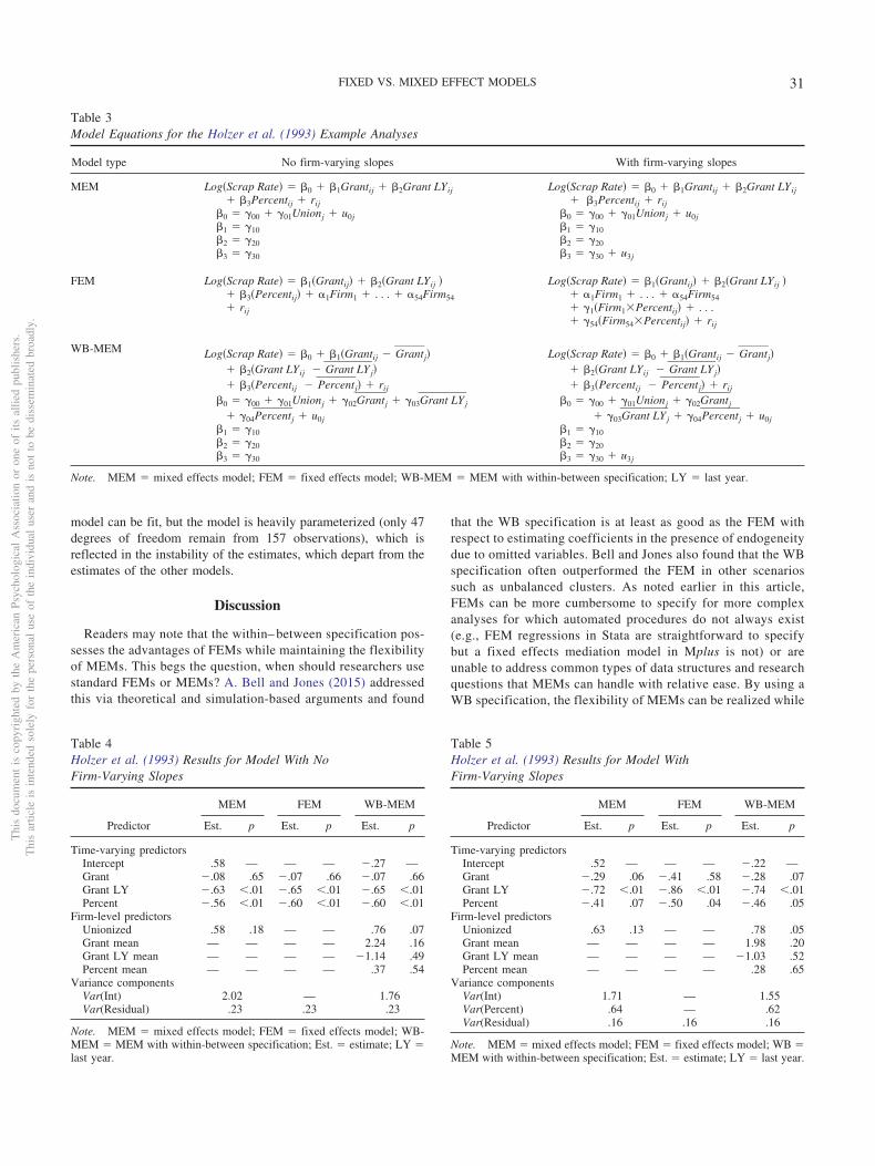
Table 4 shows the results for the three different model typeswith the predictors not being allowed to vary across firms. Gen-erally, the results show that receiving a grant in the previous yearand having a higher percentage of workers receiving trainingdecreased the number of scrapped items. Although not egregious,the results do show some possible effects of endogeneity based ona comparison of coefficients across models. If all relevant Level 2predictors were included, the effects of the traditional MEM wouldalign with the WB-MEM specifications because the alternativespecification would have no advantages, as the standard MEMwould meet all requirements of the exogeneity assumption. In theMEM, the effect of union is positive but not significant. However,in the WB specification, the effect of union is notably larger (0.58vs. 0.76, a 30% increase), though the effect remains nonsignificantand may be due to sampling error. As expected, the time-varyingeffects are identical between the FEM and WB-MEM specifica-tions, demonstrating that both specifications account for endoge-neity. As an added benefit, the WB-MEM specification allowsresearchers to estimate and test the union effect, which is notpossible in the FEM (although the FEM does control for union).

With Firm-Varying Slopes

Table 5 shows the results for the models allowing the effect ofpercent to vary across firms. In the MEM and WB specifications,the variance for this random effect was statistically significantusing a 50:50 mixture chi-square test, as recommended by Verbekeand Molenberghs (2003). The omnibus test for the Percent � Firminteraction was also significant in the FEM. In Table 5, thecomparison of the results for MEM and WB specifications followsa similar pattern to Table 4: The union effect is noticeably differentbetween specifications. The union effect in the MEM is smallerand not statistically significant, whereas the effect is notably largerand statistically significant in the WB model. A similar pattern isfound with the percent predictor. In this model, the FEM isestimating 110 parameters (two time-varying covariates, 54 firmintercepts, 54 percent slopes) from 157 total observations. The

Thi

sdo

cum

ent

isco

pyri

ghte

dby

the

Am

eric

anPs

ycho

logi

cal

Ass

ocia

tion

oron

eof

itsal

lied

publ

ishe

rs.

Thi

sar

ticle

isin

tend

edso

lely

for

the

pers

onal

use

ofth

ein

divi

dual

user

and

isno

tto

bedi

ssem

inat

edbr

oadl

y.

30 MCNEISH AND KELLEY

model can be fit, but the model is heavily parameterized (only 47degrees of freedom remain from 157 observations), which isreflected in the instability of the estimates, which depart from theestimates of the other models.

Discussion

Readers may note that the within– between specification pos-sesses the advantages of FEMs while maintaining the flexibilityof MEMs. This begs the question, when should researchers usestandard FEMs or MEMs? A. Bell and Jones (2015) addressedthis via theoretical and simulation-based arguments and found

that the WB specification is at least as good as the FEM withrespect to estimating coefficients in the presence of endogeneitydue to omitted variables. Bell and Jones also found that the WBspecification often outperformed the FEM in other scenariossuch as unbalanced clusters. As noted earlier in this article,FEMs can be more cumbersome to specify for more complexanalyses for which automated procedures do not always exist(e.g., FEM regressions in Stata are straightforward to specifybut a fixed effects mediation model in Mplus is not) or areunable to address common types of data structures and researchquestions that MEMs can handle with relative ease. By using aWB specification, the flexibility of MEMs can be realized while

Table 3Model Equations for the Holzer et al. (1993) Example Analyses

Model type No firm-varying slopes With firm-varying slopes

MEM Log�Scrap Rate� � �0 � �1Grantij � �2Grant LYij� �3Percentij � rij

�0 � �00 � �01Unionj � u0j�1 � �10�2 � �20�3 � �30

Log�Scrap Rate� � �0 � �1Grantij � �2Grant LYij� �3Percentij � rij

�0 � �00 � �01Unionj � u0j�1 � �10�2 � �20�3 � �30 � u3j

FEM Log�Scrap Rate� � �1�Grantij� � �2�Grant LYij �� �3�Percentij� � �1Firm1 � . . . � �54Firm54� rij

Log�Scrap Rate� � �1�Grantij� � �2�Grant LYij �� �1Firm1 � . . . � �54Firm54� �1�Firm1�Percentij� � . . .� �54�Firm54�Percentij� � rij

WB-MEM Log�Scrap Rate� � �0 � �1�Grantij Grant�j�� �2�Grant LYij Grant LY�j�� �3�Percentij Percent�j� � rij

�0 � �00 � �01Unionj � �02Grant�j � �03Grant LY�j

� �04Percent�j � u0j�1 � �10�2 � �20�3 � �30

Log�Scrap Rate� � �0 � �1�Grantij Grant�j�� �2�Grant LYij Grant LY�j�� �3�Percentij Percent�j� � rij

�0 � �00 � �01Unionj � �02Grant�j

� �03Grant LY�j � �04Percent�j � u0j�1 � �10�2 � �20�3 � �30 � u3j

Note. MEM � mixed effects model; FEM � fixed effects model; WB-MEM � MEM with within-between specification; LY � last year.

Table 4Holzer et al. (1993) Results for Model With NoFirm-Varying Slopes

Predictor

MEM FEM WB-MEM

Est. p Est. p Est. p

Time-varying predictorsIntercept .58 — — — �.27 —Grant �.08 .65 �.07 .66 �.07 .66Grant LY �.63 �.01 �.65 �.01 �.65 �.01Percent �.56 �.01 �.60 �.01 �.60 �.01

Firm-level predictorsUnionized .58 .18 — — .76 .07Grant mean — — — — 2.24 .16Grant LY mean — — — — �1.14 .49Percent mean — — — — .37 .54

Variance componentsVar(Int) 2.02 — 1.76Var(Residual) .23 .23 .23

Note. MEM � mixed effects model; FEM � fixed effects model; WB-MEM � MEM with within-between specification; Est. � estimate; LY �last year.

Table 5Holzer et al. (1993) Results for Model WithFirm-Varying Slopes

Predictor

MEM FEM WB-MEM

Est. p Est. p Est. p

Time-varying predictorsIntercept .52 — — — �.22 —Grant �.29 .06 �.41 .58 �.28 .07Grant LY �.72 �.01 �.86 �.01 �.74 �.01Percent �.41 .07 �.50 .04 �.46 .05

Firm-level predictorsUnionized .63 .13 — — .78 .05Grant mean — — — — 1.98 .20Grant LY mean — — — — �1.03 .52Percent mean — — — — .28 .65

Variance componentsVar(Int) 1.71 — 1.55Var(Percent) .64 — .62Var(Residual) .16 .16 .16

Note. MEM � mixed effects model; FEM � fixed effects model; WB �MEM with within-between specification; Est. � estimate; LY � last year.

Thi

sdo

cum

ent

isco

pyri

ghte

dby

the

Am

eric

anPs

ycho

logi

cal

Ass

ocia

tion

oron

eof

itsal

lied

publ

ishe

rs.

Thi

sar

ticle

isin

tend

edso

lely

for

the

pers

onal

use

ofth

ein

divi

dual

user

and

isno

tto

bedi

ssem

inat

edbr

oadl

y.

31FIXED VS. MIXED EFFECT MODELS

simultaneously estimating Level 1 effects that are protectedfrom threats of omitted variables, at least to the extent that suchprotection is afforded by FEMs. With the WB specification,researchers do not have to consciously disregard aspects likecluster-varying effects or mediation hypotheses—these can beframed within the WB specification. More directly, MEMs canvery often be specified in a way that can encompass the benefitsof FEMs while also maintaining the flexibility to assess moretypes of and more complex research interests.

If researchers are weary of the assumptions made by includ-ing random effects, Dieleman and Templin (2014) also note thatthe WB specification does not necessarily require that cluster-ing be accommodated with MEM—the WB specification can beadapted for use with cluster-robust errors or generalized esti-mating equations, such that omitted confounder bias can besimilarly guarded against if clustering is accommodated withdesign-based methods. As has been argued (e.g., Beck & Katz,2001; A. Bell & Jones, 2015; Castellano, Rabe-Hesketh, &Skrondal, 2014), the information that is being discarded inFEMs can often explain phenomena of interest; indeed, anMEM approach would allow a richer set of questions to beaddressed. It is unwise to merely control for the entirety ofLevel 2 when there are straightforward ways to incorporatesuch information into the model and preserve access to researchquestions addressing Level 2 effects.

As studies continue to stray from the classic controlled ex-periment and as nonrandom samples continue to be collected,endogeneity increasingly threatens the validity of claims madeby researchers. Given the increasingly interwoven and complexprocesses that are modeled in modern psychological research,omitted confounders are a genuine concern and researchersfrom the psychological tradition would be wise to adopt someeconometric tools and concerns. Altering MEMs ever soslightly so that they form a WB-MEM specification could go along way to address the impact of endogeneity issues have hadon models for psychological data. Additionally, such a speci-fication would allow more flexibility for econometricallygrounded researchers accustomed to employing the FEM frame-work. This type of cross-fertilization of methods presents ad-vantages for a wide variety of researchers, similar to the emer-gence of structural equation modeling framework that arosefrom blending structural models from economics with factormodels from psychology, forming a stronger overall modelingframework.

Despite the high praise given to the WB-MEM specification,it is not a universal solution for modeling clustered data. Asnoted in McNeish and Stapleton (2016), the performance ofMEMs, including the WB specification, are adversely affectedby small samples. Both A. Bell and Jones (2015) and McNeishand Stapleton (2016) recommended a FEM when the number ofLevel 2 units is small. In such cases, the data are often notsufficiently rich to support the more ambitious WB-MEM spec-ification (Maas & Hox, 2005; Stegmueller, 2013). The randomeffects in a WB-MEM also assume random sampling of clusters.Should this assumption be inappropriate, the assumption could becircumvented with an FEM because no such assumption is required inthe FEM framework. Alternatively, design-based methods like gen-eralized estimating equations can accommodate a WB specificationthat preserves Level 2 predictors without modeling with random

effects. The WB-MEM specification also does not solve all issueswith endogeneity. If researchers are trying to estimate treatmenteffects, endogeneity can occur when treatment and controlgroups are nonrandom or self-selected (e.g., only poorly per-forming employees are eligible for selection into the treatmentgroup). Endogeneity, in this case, is attributable to properties ofthe research design, measurement errors, and/or the data col-lection, not due to the way the data are modeled (A. Bell &Jones, 2015; Kennedy, 2008; Li, 2011). Neither the WB spec-ification nor the FEM address endogeneity attributable to theresearch design, and any estimated treatment effects using thesemethods would still be likely to contain bias—WB-MEM andFEMs primarily address endogeneity introduced from omissionof Level 2 variables. For endogeneity of this type, researcherscould condition on covariates (e.g., ANCOVA), use propensityscore methods, or use instrumental variables to accommodatethe endogeneity present in the variables themselves. Consistentwith the overall theme of this article, the instrumental variablesapproach is another method that is well known by researcherstrained in the econometric tradition but is not used by manyresearchers with backgrounds in psychology. The details con-comitant with instrumental variables is beyond the scope of thisarticle, so we will not address this method here—for moreinformation, see DeMaris (2014) or Foster and McLanahan(1996) for studies grounded in psychology. For more generaltreatments, see Angrist and Krueger (2001), Greenland (2000),or Heckman (1997).

In conclusion, both MEMs and FEMs have advantages thatcan provide unique benefits in the context of modeling clustereddata, whereas the WB-MEM specification is an option that canoften capitalize on advantages of both methods. Our goal hasnot been to show either method in a negative light but rather tobridge the two methods together to show how they can com-plement each other. As the line distinguishing psychology fromeconomics continues to be blurred, it is beneficial for both typesof researchers to leverage the best methodologies availableacross both fields. Different disciplines often emphasize differ-ent aspects of the same type of analyses, so integrating thesedifferent perspectives can only serve to strengthen analyses inall disciplines. Sometimes, the lack of awareness to a certainapproach is not because it is not appropriate but simply becauseit is not discussed in key training materials. We hope this articlehelps to facilitate more understanding and awareness of theavailable models.

References

Adjerid, I., & Kelley, K. (2018). Big data in psychology: A framework forresearch advancement. American Psychologist. Advance online publica-tion. http://dx.doi.org/10.1037/amp0000190

Allison, P. D. (2009). Fixed effects regression models. Thousand Oaks,CA: Sage. http://dx.doi.org/10.4135/9781412993869

Angrist, J. D., & Krueger, A. B. (2001). Instrumental variables and thesearch for identification: From supply and demand to natural experi-ments. Journal of Economic Perspectives, 15, 69–85.

Antonakis, J. (2017). On doing better science: From thrill of discovery topolicy implications. The Leadership Quarterly, 28, 5–21.

Antonakis, J., Bendahan, S., Jacquart, P., & Lalive, R. (2010). On makingcausal claims: A review and recommendations. The Leadership Quar-terly, 21, 1086–1120.

Thi

sdo

cum

ent

isco

pyri

ghte

dby

the

Am

eric

anPs

ycho

logi

cal

Ass

ocia

tion

oron

eof

itsal

lied

publ

ishe

rs.

Thi

sar

ticle

isin

tend

edso

lely

for

the

pers

onal

use

ofth

ein

divi

dual

user

and

isno

tto

bedi

ssem

inat

edbr

oadl

y.

32 MCNEISH AND KELLEY

Antonakis, J., Bendahan, S., Jacquart, P., & Lalive, R. (2014). Causalityand endogeneity: Problems and solutions. In D. V. Day (Ed.), TheOxford handbook of leadership and organizations (pp. 93–117). NewYork, NY: Oxford University Press.

Baldwin, S. A., & Fellingham, G. W. (2013). Bayesian methods for theanalysis of small sample multilevel data with a complex variance struc-ture. Psychological Methods, 18, 151–164. http://dx.doi.org/10.1037/a0030642

Baltagi, B. (2013). Econometric analysis of panel data. New York, NY:Wiley.

Bates, D. M. (2010). lme4: Mixed-effects modeling with R. Retrieved fromhttp://lme4.r-forge.r-project.org/book/

Bauer, D. J., Preacher, K. J., & Gil, K. M. (2006). Conceptualizing andtesting random indirect effects and moderated mediation in multilevelmodels: New procedures and recommendations. PsychologicalMethods, 11, 142–163. http://dx.doi.org/10.1037/1082-989X.11.2.142

Bauer, D. J., & Sterba, S. K. (2011). Fitting multilevel models with ordinaloutcomes: Performance of alternative specifications and methods ofestimation. Psychological Methods, 16, 373–390. http://dx.doi.org/10.1037/a0025813

Beck, N., & Katz, J. N. (2001). Throwing out the baby with the bath water:A comment on Green, Kim, and Yoon. International Organization, 55,487–495. http://dx.doi.org/10.1162/00208180151140658

Bell, A., & Jones, K. (2015). Explaining fixed effects: Random effectsmodeling of time-series cross-sectional and panel data. Political ScienceResearch and Methods, 3, 133–153. http://dx.doi.org/10.1017/psrm.2014.7

Bell, B., Morgan, G., Schoeneberger, J. B., Kromrey, J., & Ferron, J.(2014). How low can you go? An investigation of the influence ofsample size and model complexity on point and interval estimates intwo-level linear models. Methodology: European Journal of ResearchMethods for the Behavioral and Social Sciences, 10, 1–11. http://dx.doi.org/10.1027/1614-2241/a000062

Bollen, K., & Curran, P. (2006). Latent curve models: A structural equa-tion perspective. New York, NY: Wiley.

Bryk, A. S., & Raudenbush, S. W. (1988). Toward a more appropriateconceptualization of research on school effects: A three-level hierarchi-cal linear model. American Journal of Education, 97, 65–108. http://dx.doi.org/10.1086/443913

Castellano, K. E., Rabe-Hesketh, S., & Skrondal, A. (2014). Composition,context, and endogeneity in school and teacher comparisons. Journal ofEducational and Behavioral Statistics, 39, 333–367. http://dx.doi.org/10.3102/1076998614547576

Clark, T. S., & Linzer, D. A. (2015). Should I use fixed or random effects?Political Science Research and Methods, 3, 399–408.

Dedrick, R. F., Ferron, J. M., Hess, M. R., Hogarty, K. Y., Kromrey,J. D., Lang, T. R., . . . Lee, R. (2009). Multilevel modeling: A reviewof methodological issues and applications. Review of EducationalResearch, 79, 69 –102. http://dx.doi.org/10.3102/0034654308325581

DeMaris, A. (2014). Combating unmeasured confounding in cross-sectional studies: Evaluating instrumental-variable and Heckman selec-tion models. Psychological Methods, 19, 380–397. http://dx.doi.org/10.1037/a0037416

Dieleman, J. L., & Templin, T. (2014). Random-effects, fixed-effects andthe within-between specification for clustered data in observationalhealth studies: A simulation study. PLoS ONE, 9, e110257. http://dx.doi.org/10.1371/journal.pone.0110257

Ebbes, P., Wedel, M., Böckenholt, U., & Steerneman, T. (2005). Solvingand testing for regressor-error (in) dependence when no instrumentalvariables are available: With new evidence for the effect of education onincome. Quantitative Marketing and Economics, 3, 365–392. http://dx.doi.org/10.1007/s11129-005-1177-6

Enders, C. K., & Tofighi, D. (2007). Centering predictor variables incross-sectional multilevel models: A new look at an old issue. Psycho-logical Methods, 12, 121–138. http://dx.doi.org/10.1037/1082-989X.12.2.121

Feaster, D., Brincks, A., Robbins, M., & Szapocznik, J. (2011). Multilevelmodels to identify contextual effects on individual group member out-comes: A family example. Family Process, 50, 167–183. http://dx.doi.org/10.1111/j.1545-5300.2011.01353.x

Ferron, J. M., Bell, B. A., Hess, M. R., Rendina-Gobioff, G., &Hibbard, S. T. (2009). Making treatment effect inferences frommultiple-baseline data: The utility of multilevel modeling ap-proaches. Behavior Research Methods, 41, 372–384. http://dx.doi.org/10.3758/BRM.41.2.372

Ferron, J., Hogarty, K., Dedrick, R., Hess, M., Niles, J., & Kromrey, J.(2008). Reporting results from multilevel analyses. In A. O’Connell &B. McCoach (Eds.), Multilevel analysis of educational data (pp. 391–426). Charlotte, NC: Information Age Publishing.

Foster, E. M., & McLanahan, S. (1996). An illustration of the use ofinstrumental variables: Do neighborhood conditions affect a youngperson’s chance of finishing high school? Psychological Methods, 1,249 –260. http://dx.doi.org/10.1037/1082-989X.1.3.249

Gardiner, J. C., Luo, Z., & Roman, L. A. (2009). Fixed effects, randomeffects and GEE: What are the differences? Statistics in Medicine, 28,221–239. http://dx.doi.org/10.1002/sim.3478

Gelman, A. (2006). Prior distributions for variance parameters in hierar-chical models (comment on article by Browne and Draper). BayesianAnalysis, 1, 515–534. http://dx.doi.org/10.1214/06-BA117A

Gelman, A., & Hill, J. (2006). Data analysis using regression and multi-level/hierarchical models. Cambridge, MA: Cambridge UniversityPress. http://dx.doi.org/10.1017/CBO9780511790942

Goldstein, H. (1986). Multilevel mixed linear model analysis using itera-tive generalized least squares. Biometrika, 73, 43–56. http://dx.doi.org/10.1093/biomet/73.1.43

Goldstein, H. (1989). Restricted unbiased iterative generalized least-squares estimation. Biometrika, 76, 622–623. http://dx.doi.org/10.1093/biomet/76.3.622

Grady, M. W., & Beretvas, S. N. (2010). Incorporating student mobility inachievement growth modeling: A cross-classified multiple membershipgrowth curve model. Multivariate Behavioral Research, 45, 393–419.http://dx.doi.org/10.1080/00273171.2010.483390

Greene, W. (2003). Econometric analysis. Upper Saddle River, NJ: Pren-tice Hall.

Greenland, S. (2000). An introduction to instrumental variables for epide-miologists. International Journal of Epidemiology, 29, 722–729. http://dx.doi.org/10.1093/ije/29.4.722

Halaby, C. N. (2004). Panel models in sociological research: Theory intopractice. Annual Review of Sociology, 30, 507–544.

Harville, D. A. (1977). Maximum likelihood approaches to variance com-ponent estimation and to related problems. Journal of the AmericanStatistical Association, 72, 320 –338. http://dx.doi.org/10.1080/01621459.1977.10480998

Hayes, A. F. (2013). Introduction to mediation, moderation, and condi-tional process analysis: A regression-based approach. New York, NY:Guilford Press.

Heckman, J. (1997). Instrumental variables: A study of implicit behavioralassumptions used in making program evaluations. The Journal of Hu-man Resources, 32, 441–462. http://dx.doi.org/10.2307/146178

Hofmann, D. A., & Gavin, M. B. (1998). Centering decisions in hierar-chical linear models: Implications for research in organizations. Journalof Management, 24, 623–641. http://dx.doi.org/10.1177/014920639802400504

Holzer, H. J., Block, R. N., Cheatham, M., & Knott, J. H. (1993). Aretraining subsidies for firms effective? The Michigan experience. Indus-

Thi

sdo

cum

ent

isco

pyri

ghte

dby

the

Am

eric

anPs

ycho

logi

cal

Ass

ocia

tion

oron

eof

itsal

lied

publ

ishe

rs.

Thi

sar

ticle

isin

tend

edso

lely

for

the

pers

onal

use

ofth

ein

divi

dual

user

and

isno

tto

bedi

ssem

inat

edbr

oadl

y.

33FIXED VS. MIXED EFFECT MODELS

trial & Labor Relations Review, 46, 625–636. http://dx.doi.org/10.1177/001979399304600403

Hox, J. (2010). Multilevel analysis: Techniques and applications. Mahwah,NJ: Erlbaum.

Hox, J. J., van de Schoot, R., & Matthijsse, S. (2012). How few countrieswill do? Comparative survey analysis from a Bayesian perspective.Survey Research Methods, 6, 87–93.

Hsiao, C. (2003). Analysis of panel data. Cambridge, UK: CambridgeUniversity Press. http://dx.doi.org/10.1017/CBO9780511754203

Huang, F. (2016). Alternatives to multilevel modeling for the analysis ofclustered data. Journal of Experimental Education, 84, 175–196. http://dx.doi.org/10.1080/00220973.2014.952397

Judge, G. G., Griffiths, W. E., Hill, R. C., & Lee, T. C. (1985). The theoryand practice of econometrics. New York, NY: Wiley.

Kennedy, P. (2008). A guide to econometrics. Malden, MA: Blackwell.Kenny, D. A., Korchmaros, J. D., & Bolger, N. (2003). Lower level

mediation in multilevel models. Psychological Methods, 8, 115–128.http://dx.doi.org/10.1037/1082-989X.8.2.115

Kenward, M. G., & Roger, J. H. (1997). Small sample inference for fixedeffects from restricted maximum likelihood. Biometrics, 53, 983–997.http://dx.doi.org/10.2307/2533558

Kim, J., & Frees, E. W. (2006). Omitted variables in multilevel models.Psychometrika, 71, 659 – 690. http://dx.doi.org/10.1007/s11336-005-1283-0

Kim, J., & Frees, E. W. (2007). Multilevel modeling with correlatedeffects. Psychometrika, 72, 505–533. http://dx.doi.org/10.1007/s11336-007-9008-1

Kim, J. S., & Swoboda, C. M. (2010). Handling omitted variable bias inmultilevel models: Model specification tests and robust estimation. InJ. J. Hox & J. K. Roberts (Eds.), Handbook of advanced multilevelanalysis (pp. 197–217). New York, NY: Routledge.

Kreft, I. G., de Leeuw, J., & Aiken, L. S. (1995). The effect of differentforms of centering in hierarchical linear models. Multivariate Behav-ioral Research, 30, 1–21. http://dx.doi.org/10.1207/s15327906mbr3001_1

Krull, J. L., & MacKinnon, D. P. (1999). Multilevel mediation modeling ingroup-based intervention studies. Evaluation Review, 23, 418–444.http://dx.doi.org/10.1177/0193841X9902300404

Laird, N. M., & Ware, J. H. (1982). Random-effects models for longitu-dinal data. Biometrics, 38, 963–974. http://dx.doi.org/10.2307/2529876

Li, X. (2011). Approaches to modelling heterogeneity in longitudinalstudies. Wellington, New Zealand: Victoria University.

Liang, K. Y., & Zeger, S. L. (1986). Longitudinal data analysis usinggeneralized linear models. Biometrika, 73, 13–22. http://dx.doi.org/10.1093/biomet/73.1.13

Maas, C. J., & Hox, J. J. (2005). Sufficient sample sizes for multilevelmodeling. Methodology: European Journal of Research Methods for theBehavioral and Social Sciences, 1, 86–92. http://dx.doi.org/10.1027/1614-2241.1.3.86

Maxwell, S. E., Delaney, H. D., & Kelley, K. (2018). Designing experi-ments and analyzing data: A model comparison perspective. New York,NY: Routledge.

McNeish, D. (2016). On using Bayesian methods to address small sampleproblems. Structural Equation Modeling, 23, 750–773. http://dx.doi.org/10.1080/10705511.2016.1186549

McNeish, D. (2017a). Challenging conventional wisdom for multivariatestatistical models with small samples. Review of Educational Research,87, 1117–1151. http://dx.doi.org/10.3102/0034654317727727

McNeish, D. (2017b). Small sample methods for multilevel modeling: Acolloquial elucidation of REML and the Kenward-Roger correction.Multivariate Behavioral Research, 52, 661–670. http://dx.doi.org/10.1080/00273171.2017.1344538

McNeish, D., & Stapleton, L. M. (2016). Modeling clustered data with veryfew clusters. Multivariate Behavioral Research, 51, 495–518. http://dx.doi.org/10.1080/00273171.2016.1167008

McNeish, D., Stapleton, L. M., & Silverman, R. D. (2017). On theunnecessary ubiquity of hierarchical linear modeling. PsychologicalMethods, 22, 114–140. http://dx.doi.org/10.1037/met0000078

McNeish, D., & Wentzel, K. R. (2017). Accommodating small samplesizes in three-level models when the third level is incidental. Multivar-iate Behavioral Research, 52, 200 –215. http://dx.doi.org/10.1080/00273171.2016.1262236

Meyers, J. L., & Beretvas, S. N. (2006). The impact of inappropriatemodeling of cross-classified data structures. Multivariate BehavioralResearch, 41, 473– 497. http://dx.doi.org/10.1207/s15327906mbr4104_3

Moulton, B. R. (1986). Random group effects and the precision of regres-sion estimates. Journal of Econometrics, 32, 385–397. http://dx.doi.org/10.1016/0304-4076(86)90021-7

Moulton, B. R. (1990). An illustration of a pitfall in estimating the effectsof aggregate variables on micro units. The Review of Economics andStatistics, 72, 334–338. http://dx.doi.org/10.2307/2109724

Mundlak, Y. (1978). On the pooling of time series and cross section data.Econometrica, 46, 69–85. http://dx.doi.org/10.2307/1913646

Patterson, H. D., & Thompson, R. (1971). Recovery of inter-block infor-mation when block sizes are unequal. Biometrika, 58, 545–554. http://dx.doi.org/10.1093/biomet/58.3.545

Petersen, M. A. (2009). Estimating standard errors in finance panel datasets: Comparing approaches. Review of Financial Studies, 22, 435–480.http://dx.doi.org/10.1093/rfs/hhn053

Plümper, T., & Troeger, V. E. (2007). Efficient estimation of time-invariant and rarely changing variables in finite sample panel analyseswith unit fixed effects. Political Analysis, 15, 124–139. http://dx.doi.org/10.1093/pan/mpm002

Preacher, K. J. (2011). Multilevel SEM strategies for evaluating mediationin three-level data. Multivariate Behavioral Research, 46, 691–731.http://dx.doi.org/10.1080/00273171.2011.589280

Preacher, K. J., Curran, P. J., & Bauer, D. J. (2006). Computationaltools for probing interactions in multiple linear regression, multilevelmodeling, and latent curve analysis. Journal of Educational andBehavioral Statistics, 31, 437– 448. http://dx.doi.org/10.3102/10769986031004437

Preacher, K. J., Zyphur, M. J., & Zhang, Z. (2010). A general multilevelSEM framework for assessing multilevel mediation. PsychologicalMethods, 15, 209–233. http://dx.doi.org/10.1037/a0020141

Rabe-Hesketh, S., & Skrondal, A. (2008). Multilevel and longitudinalmodeling using Stata. Berkeley, CA: Stata Press.

Raudenbush, S., & Bryk, A. S. (1986). A hierarchical model for studyingschool effects. Sociology of Education, 59, 1–17. http://dx.doi.org/10.2307/2112482

Raudenbush, S. W., & Bryk, A. S. (2002). Hierarchical linear models:Applications and data analysis methods. Thousand Oaks, CA: Sage.

Schurer, S., & Yong, J. (2012). Personality, well-being and the marginalutility of income: What can we learn from random coefficient models?Health, Econometrics and Data Group (HEDG) Working Papers. De-partment of Economics, University of York, York, United Kingdom.

Singer, J. D., & Willett, J. B. (2003). Applied longitudinal data analysis:Modeling change and event occurrence. New York, NY: Oxford Uni-versity Press. http://dx.doi.org/10.1093/acprof:oso/9780195152968.001.0001

Snijders, T. A. B., & Bosker, R. J. (2012). Multilevel analysis. London,UK: Sage.

Stegmueller, D. (2013). How many countries for multilevel modeling?A comparison of frequentist and Bayesian approaches. AmericanJournal of Political Science, 57, 748 –761. http://dx.doi.org/10.1111/ajps.12001

Thi

sdo

cum

ent

isco

pyri

ghte

dby

the

Am

eric

anPs

ycho

logi

cal

Ass

ocia

tion

oron

eof

itsal

lied

publ

ishe

rs.

Thi

sar

ticle

isin

tend

edso

lely

for

the

pers

onal

use

ofth

ein

divi

dual

user

and

isno

tto

bedi

ssem

inat

edbr

oadl

y.

34 MCNEISH AND KELLEY

Stiratelli, R., Laird, N., & Ware, J. H. (1984). Random-effects models forserial observations with binary response. Biometrics, 40, 961–971.http://dx.doi.org/10.2307/2531147

Stram, D. O., & Lee, J. W. (1994). Variance components testing in thelongitudinal mixed effects model. Biometrics, 50, 1171–1177. http://dx.doi.org/10.2307/2533455

Tofighi, D., & Kelley, K. (2016). Assessing omitted confounder bias inmultilevel mediation models. Multivariate Behavioral Research, 51,86–105. http://dx.doi.org/10.1080/00273171.2015.1105736

Verbeke, G., & Molenberghs, G. (2003). The use of score tests forinference on variance components. Biometrics, 59, 254–262. http://dx.doi.org/10.1111/1541-0420.00032

Wooldridge, J. M. (2002). Econometric analysis of cross section and paneldata. Cambridge, MA: MIT Press.

Wooldridge, J. M. (2003). Cluster-sample methods in applied economet-rics. The American Economic Review, 93, 133–138. http://dx.doi.org/10.1257/000282803321946930

Yang, Y., & Land, K. C. (2008). Age -period -cohort analysis of repeatedcross-section surveys: fixed or random effects? Sociological Methods &Research, 36, 297–326.

Zhang, Z., Zyphur, M. J., & Preacher, K. J. (2009). Testing multilevelmediation using hierarchical linear models problems and solutions.Organizational Research Methods, 12, 695–719. http://dx.doi.org/10.1177/1094428108327450

Received January 17, 2017Revision received January 5, 2018

Accepted January 25, 2018 �

Thi

sdo

cum

ent

isco

pyri

ghte

dby

the

Am

eric

anPs

ycho

logi

cal

Ass

ocia

tion

oron

eof

itsal

lied

publ

ishe

rs.

Thi

sar

ticle

isin

tend

edso

lely

for

the

pers

onal

use

ofth

ein

divi

dual

user

and

isno

tto

bedi

ssem

inat

edbr

oadl

y.

35FIXED VS. MIXED EFFECT MODELS