Five-Year Evaluation of the Hass Avocado Board’s ... · fresh avocados. The elasticity of demand...
56
Five-Year Evaluation of the Hass Avocado Board’s Promotional Programs: 2008 - 2012 Hoy F. Carman Tina L. Saitone Richard J. Sexton 1 September 2013 1 Hoy F. Carman is Professor Emeritus, Tina L. Saitone is Project Economist, and Richard J. Sexton is Professor and Chair, Department of Agricultural and Resource Economics, University of California, Davis.
Transcript of Five-Year Evaluation of the Hass Avocado Board’s ... · fresh avocados. The elasticity of demand...
Five-Year Evaluation of the Hass Avocado Board’s
Promotional Programs: 2008 - 2012
Hoy F. Carman Tina L. Saitone
Richard J. Sexton1
September 2013
1 Hoy F. Carman is Professor Emeritus, Tina L. Saitone is Project Economist, and Richard J. Sexton is Professor and Chair, Department of Agricultural and Resource Economics, University of California, Davis.
1
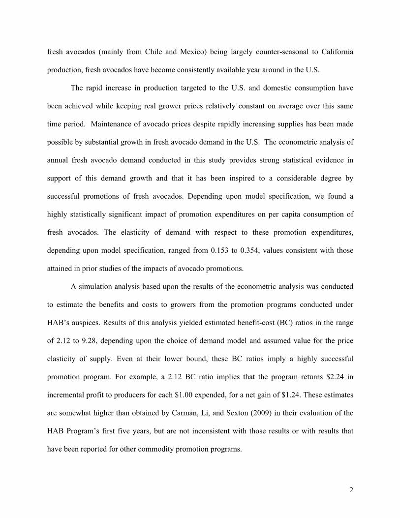
Executive Summary This report represents the second quinquennial evaluation of the promotion programs conducted
under the auspices of the Hass Avocado Board (HAB) as authorized by the Hass Avocado
Promotion, Research, and Information Act enacted into law in October 2000. The first five-year
review, conducted by Carman, Li, and Sexton (CLS 2009), covered the period from 2003
through 2007. CLS found that advertising and promotion funded under the HAB increased the
demand for fresh avocados during the program’s first five years of operation and yielded a
favorable rate of return for the assessment dollars invested by avocado producers and importers.
This evaluation focuses upon activities conducted under the auspices of the HAB from
2008 through 2012. The evaluation involved four central components: (i) review and assessment
of recent trends in sales, prices, and promotions of fresh avocados in the U.S. market (section 3);
(ii) a descriptive analysis of the amounts expended and the nature of expenditures by each of the
groups participating in the program, the California Avocado Commission, the Chilean Avocado
Importers Association, the Mexican Hass Avocado Importers Association, the Peruvian Avocado
Commission, and HAB itself (section 4); (iii) econometric analysis of annual fresh avocado
demand for the 19-year period from 1994 – 2012 (section 6); and (iv) econometric analysis of
weekly fresh avocado sales at retail for 2008 – 2012 using scanner data for 38 designated
marketing areas (section 8).
Fresh avocado consumption has grown rapidly in the U.S., rising from about 1.5 pound
per capita during the decade of the 1990s to over 5.0 pounds per capita in 2012. This growth in
consumption and supplies within the U.S. market has coincided with growing market share for
imports, rising from 30 percent of total supplies in 2000 to 67 percent in 2012. With imports of
2
fresh avocados (mainly from Chile and Mexico) being largely counter-seasonal to California
production, fresh avocados have become consistently available year around in the U.S.
The rapid increase in production targeted to the U.S. and domestic consumption have
been achieved while keeping real grower prices relatively constant on average over this same
time period. Maintenance of avocado prices despite rapidly increasing supplies has been made
possible by substantial growth in fresh avocado demand in the U.S. The econometric analysis of
annual fresh avocado demand conducted in this study provides strong statistical evidence in
support of this demand growth and that it has been inspired to a considerable degree by
successful promotions of fresh avocados. Depending upon model specification, we found a
highly statistically significant impact of promotion expenditures on per capita consumption of
fresh avocados. The elasticity of demand with respect to these promotion expenditures,
depending upon model specification, ranged from 0.153 to 0.354, values consistent with those
attained in prior studies of the impacts of avocado promotions.
A simulation analysis based upon the results of the econometric analysis was conducted
to estimate the benefits and costs to growers from the promotion programs conducted under
HAB’s auspices. Results of this analysis yielded estimated benefit-cost (BC) ratios in the range
of 2.12 to 9.28, depending upon the choice of demand model and assumed value for the price
elasticity of supply. Even at their lower bound, these BC ratios imply a highly successful
promotion program. For example, a 2.12 BC ratio implies that the program returns $2.24 in
incremental profit to producers for each $1.00 expended, for a net gain of $1.24. These estimates
are somewhat higher than obtained by Carman, Li, and Sexton (2009) in their evaluation of the
HAB Program’s first five years, but are not inconsistent with those results or with results that
have been reported for other commodity promotion programs.

3
Econometric analysis of scanner data containing weekly sales of fresh avocados in the 38
designated marketing areas (DMA) for 2008 – 2012 also found a positive and statistically
significant impact of targeted local/regional promotions on per capita sales in the targeted
marketing areas. Results from the scanner data analysis also provided additional insights as to
the impacts on fresh avocado consumption of price promotions, seasonality, and special holidays
and events. Price reductions in a given week were found to increase sales in that week, but the
sales improvement was fully offset by reduced purchases in subsequent weeks. Cinco de Mayo
and Independence Day were shown to be the holidays/events associated with the greatest per
capita consumption of fresh avocados, followed by Valentine’s/Presidents’ Day and Easter. May
and July had the highest per capita expenditures on fresh avocados, while the lowest
expenditures were recorded in November, December, and February.
The consistency of our results across the different analyses—evaluation of trends in
avocado consumption and prices, econometric analysis of aggregate annual demand, and
econometric analysis of disaggregate weekly demand within DMA—enable us to conclude with
considerable confidence that the promotion programs conducted under the HAB’s auspices have
been successful in expanding demand for fresh avocados in the U.S. and yielding a very
favorable return to the producers and importers funding the programs. Further, the evidence
suggests that expansion of the HAB’s promotion programs would also yield positive net benefits
from increased assessments.

4
Table of Contents
1. INTRODUCTION ............................................................................................................................... 6 2. THE HASS AVOCADO PROMOTION, RESEARCH, AND INFORMATION ACT ................ 8 3. THE CHANGING U.S. AVOCADO MARKET ............................................................................... 9 4. AVOCADO PROMOTION IN THE U.S. MARKET .................................................................... 14
4.1. CALIFORNIA AVOCADO COMMISSION PROGRAMS ....................................................................... 15 4.2. MEXICAN HASS AVOCADO IMPORTERS ASSOCIATION PROGRAMS ............................................. 16 4.3. HASS AVOCADO BOARD PROGRAMS ........................................................................................... 17 4.4. CHILEAN AVOCADO IMPORTERS ASSOCIATION PROGRAMS ........................................................ 18 4.5. PERUVIAN AVOCADO COMMISSION PROGRAMS .......................................................................... 19
5. SUMMARY OF RESULTS OF PRIOR EVALUATIONS OF AVOCADO PROMOTIONS .. 20 6. ECONOMETRIC MODELS OF THE ANNUAL DEMAND FOR AVOCADOS ..................... 22 7. COST-BENEFIT ANALYSIS OF FRESH AVOCADO PROMOTION EXPENDITURES ..... 28 8. FRESH AVOCADO DEMAND ANALYSIS AT THE RETAIL LEVEL ................................... 38
8.1. THE DATA ..................................................................................................................................... 39 8.2. MODEL SPECIFICATION ................................................................................................................ 43 8.3. RESULTS ....................................................................................................................................... 44 8.4. DISCUSSION .................................................................................................................................. 50
9. CONCLUSION .................................................................................................................................. 52
5
List of Tables Table 1. U.S. Avocado Promotional Expenditures by Organization: 2003-2012 ......................... 15 Table 2. HAB Expenditures by Category: 2008-2012 .................................................................. 18 Table 3. Correlation Coefficients for Demand Model: 1994-2012 ............................................... 24 Table 4. Variable Definitions and Summary Statistics: 1994 – 2012 ........................................... 25 Table 5. Annual Model Regression Results .................................................................................. 26 Table 6. Estimated Benefit-Cost and Grower Price Impacts from Expansion of the HAB
Promotion Program ............................................................................................................... 35 Table 7. Sales and Price Summary Statistics by DMA ................................................................. 41 Table 8. DMAs Contained in Scanner Data and Where Promotions are Conducted ................... 42 Table 9. Retail Demand Model Regression Results ..................................................................... 45 Table 10. Retail Demand Model Regression Results ................................................................... 50
List of Figures Figure 1. Sources of Fresh Avocados Supplied to the U.S. Market: 1992 -2012 ......................... 11 Figure 2. Per Capita Consumption and Real Producer Price for Fresh Avocados ....................... 12 Figure 3. Fresh and Processed Avocado Imports: 1994 - 2012 .................................................... 13 Figure 4. Avocado Promotion Simulation Model ......................................................................... 30 Figure 5. 2012 Per Capita Fresh Avocado Consumption by Month ............................................. 47 Figure 6. Per Capita Fresh Avocado Consumption During Holidays: 2012 ................................. 48
6
Five-Year Evaluation of The Hass Avocado Board’s Promotion
Programs: 2008 - 2012
1. Introduction
The U.S. demand for avocados has grown substantially in the ten years since the Hass
Avocado Board (HAB) began funding promotional programs in January 2003. Fresh
avocado supply and consumption in the U.S. has increased from an annual average of
1.51 pounds per capita during the decade of the 1990s to 5.10 pounds per capita in 2012.
This period has also seen major developments in the avocado subsector associated with
growing market share for imports (from 30 percent in 2000 to 67 percent in 2012),
increased year-round availability of fresh avocados, year-round and permanent shelf
space for avocados in retail outlets, and development of regions within the U.S., which
heretofore had limited availability and consumption of avocados, into important markets
for them. Accompanying these changes have been improvements in the distribution
system for fresh avocados including the very effective ripe avocado programs.
The farm-level demand for avocados is widely acknowledged to be quite inelastic,
with empirical estimates (including this study) typically near -0.25, depending on the
time period and variables included in the demand equation. One would thus expect
sharply lower prices to accompany an increase in avocado supply of over 200 percent.
Yet real prices have remained relatively stable on average over this period, an outcome
made possible only due to a significant increase in the demand for avocados.
Carman, Li, and Sexton (CLS 2009) conducted the first evaluation of the HAB
promotion programs for the five-year period from 2003 through 2007. CLS found that
advertising and promotion funded under the HAB increased the demand for fresh

7
avocados during the program’s first five years of operation and yielded a favorable rate of
return to avocado producers who invest in the program via assessments on their
production.
This report evaluates the economic impact of promotional expenditures conducted
under HAB’s auspices on U.S. demand for fresh avocados and estimates producer returns
from the expenditures for the second five years of the HAB’s operations, the period from
2008 through 2012. The CLS study is utilized to help guide specification and estimation
of economic models for this evaluation, and for brevity’s sake we do not repeat
discussion contained in that report.
As in CLS, we estimate both an aggregate annual model of demand for fresh
avocados in the U.S. and a disaggregate weekly demand model that relies upon retail
scanner data collected for major metropolitan areas in the U.S. that is pooled across
location for the five-year time period. A market simulation model is constructed using
results from estimation of the annual model. This model is utilized to study what-if
scenarios involving the benefits and costs of a hypothetical increase in promotion
expenditures under the auspices of the HAB to estimate the net benefits accruing to
producers from the HAB promotion programs.
In the remainder of this report, we briefly discuss the legislative history behind
the HAB and touch upon major trends impacting the Hass avocado market in the U.S. We
then turn to analysis of avocado promotion programs conducted under the HAB’s
auspices during the 2008 – 2012 period. This analysis involves three dimensions. First,
we review the expenditures and activities undertaken by HAB and the state and member
organizations that are certified by the U.S. Department of Agriculture. Second, we

8
examine the annual demand for fresh avocados in the U.S. and measure the impact of
promotion expenditures on demand. The results of this analysis are utilized to
parameterize a simulation model that is used to estimate benefits and costs to producers
from funding promotions. Finally, we conduct analysis of the retail scanner data and
evaluate the impacts of local and regional promotions on avocado demand in those
market areas.
2. The Hass Avocado Promotion, Research, and Information Act
California avocado growers’ longstanding program to fund advertising and promotion
programs for their fruit was extended to include imports of fresh avocados through the
Hass Avocado Promotion, Research, and Information Act signed into law by President
Clinton on October 23, 2000. This Act established the authorizing platform and timetable
for the creation of the Hass Avocado Promotion, Research and Information Order
(HAPRIO) that was approved in a referendum of producers and importers with 86.6
percent support on July 29, 2002.
Mandatory program assessments of 2.5 cents per pound on all Hass avocados sold
in the U.S. market commenced effective January 2, 2003 under the HAPRIO. The
assessment is collected by first handlers for California production and by the U.S.
Customs Service for imports and forwarded to the HAB. These funds are then allocated
to programs and activities designed to increase the demand for Hass avocados in the U.S.
market. The HAB uses 15 percent of the assessments to fund activities such as nutrition
research, marketing, and information programs intended to benefit all avocado producers
and rebates 85 percent of domestic assessments to the California Avocado Commission

9
(CAC) and up to 85 percent of importer assessments to the certified importer associations
for their own promotion programs. There are currently three certified importer
associations operating under the HAB: the Chilean Avocado Importers Association
(CAIA), the Mexican Hass Avocado Importers Association (MHAIA), and the Peruvian
Avocado Commission (PAC).2
Assessment income to support the activities of the HAB totaled $98.67 million
during its first five years and increased to a total $148.47 million during its second five
years. During the second five-year period, 71.5 percent of the assessments were paid on
imports and 28.5 percent were paid on California Hass avocado sales. Shares of the total
assessment paid by importers were 56.7 percent by Mexico, 13.2 percent by Chile, almost
1.0 percent by Peru, and 0.6 percent by other countries.
3. The Changing U.S. Avocado Market
Through the 1980s most avocados consumed in the U.S. were produced in California and
Florida, with only small amounts imported. For example, from 1962 through 1989
imported avocados averaged 3.16 million pounds annually and accounted for an average
of just over one percent of the total U.S. avocado supply. Then in 1990, avocado imports
jumped to nearly 26 million pounds, accounting for over nine percent of U.S. supplies.
With growing avocado acreage and production in Chile and the Dominican Republic and
with Mexico gaining limited access to the U.S. market beginning in 1997, avocado
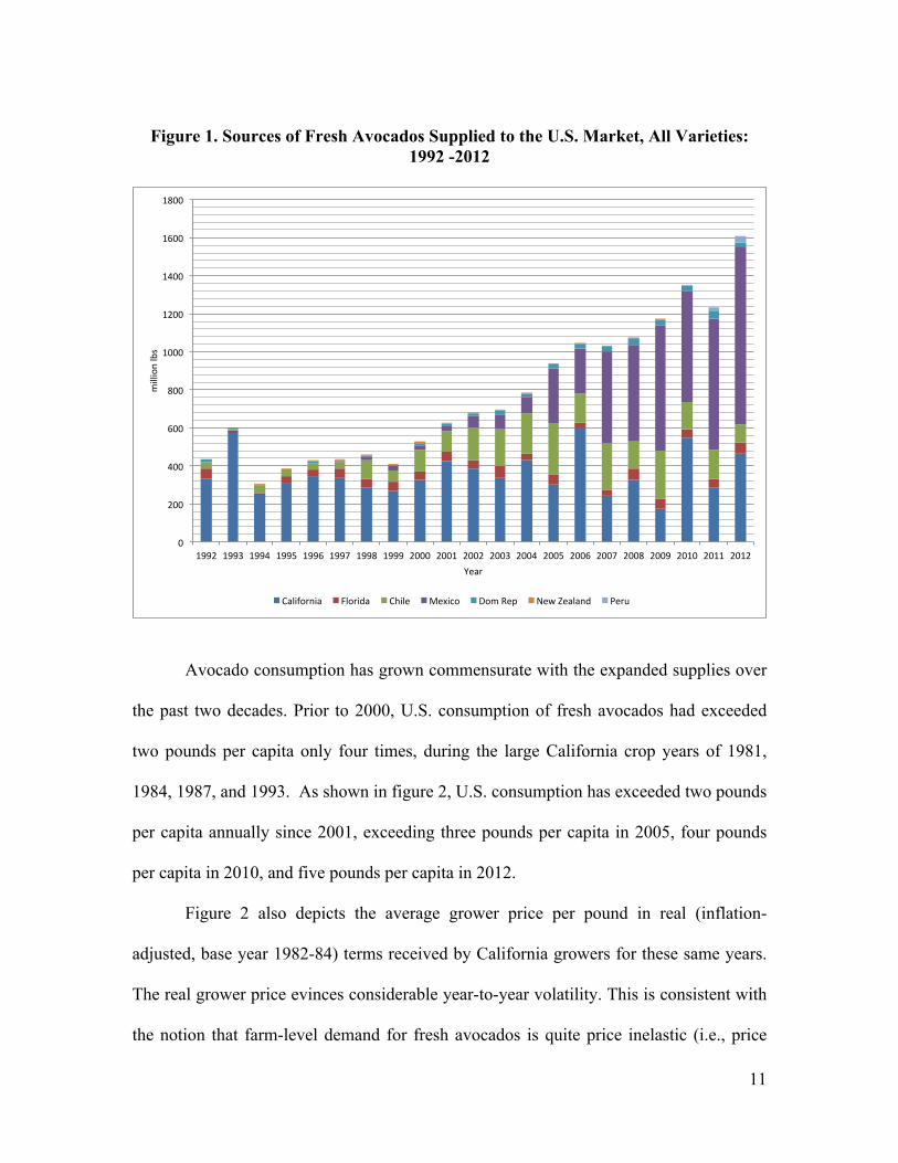
imports increased steadily (figure 1), reaching 145.98 million pounds, almost one-third of
total U.S. supplies in 2000. With Mexico’s access to the U.S. market expanding in 2001
2 Fresh avocado imports from Peru began in 2011.
10
and 2002, total Hass avocado imports increased to over 251.42 million pounds (39.5
percent of total supply) in 2002.
Since HAB assessments to support avocado promotion began in 2003, avocado
imports and total U.S. supplies (Hass and other varieties) have continued to increase to a
record total of over 1.605 billion pounds in 2012. Mexican avocado exports to the U.S.
increased significantly after Mexico gained year-round access to all states except
California and Florida in 2005 and to all states in 2007. Mexican imports of 933.8
million pounds accounted for over 58 percent of the total U.S. supply of fresh avocados
and for 86.7 percent of total fresh avocado imports in 2012 (figure 1). Chilean imports
reached a maximum of 267 million pounds in 2005 and have since varied in a range from
94 to 248 million pounds due primarily to variations in annual yields of the Chilean crop
and diversification of exports from Chile to other countries. With a small crop in 2012,
Chile’s share of total U.S. avocado imports was only 8.7 percent.
The Hass variety of avocados accounts for the vast majority of the avocados
consumed in the U.S. For example, in 2012 approximately 96.5 percent of all fresh
avocados imported to the U.S. and about 97.0 percent of California production were the
Hass variety. Florida avocado production is the only appreciable non-Hass supply in the
U.S. Overall, Hass avocados have recently accounted for about 95.0 percent of total U.S.
avocado supplies.
11
Figure 1. Sources of Fresh Avocados Supplied to the U.S. Market, All Varieties:
1992 -2012
Avocado consumption has grown commensurate with the expanded supplies over
the past two decades. Prior to 2000, U.S. consumption of fresh avocados had exceeded
two pounds per capita only four times, during the large California crop years of 1981,
1984, 1987, and 1993. As shown in figure 2, U.S. consumption has exceeded two pounds
per capita annually since 2001, exceeding three pounds per capita in 2005, four pounds
per capita in 2010, and five pounds per capita in 2012.
Figure 2 also depicts the average grower price per pound in real (inflation-
adjusted, base year 1982-84) terms received by California growers for these same years.
The real grower price evinces considerable year-to-year volatility. This is consistent with
the notion that farm-level demand for fresh avocados is quite price inelastic (i.e., price
0"
200"
400"
600"
800"
1000"
1200"
1400"
1600"
1800"
1992" 1993" 1994" 1995" 1996" 1997" 1998" 1999" 2000" 2001" 2002" 2003" 2004" 2005" 2006" 2007" 2008" 2009" 2010" 2011" 2012"
million"lbs"
Year"
California" Florida" Chile" Mexico" Dom"Rep" New"Zealand" Peru"

12
responds more than proportionally to a given percent change in crop availability).
Figure 2. Per Capita Consumption and Real Producer Price for Fresh Avocados
Yet the fact that the average real grower price has remained relatively stable in the
presence of an over 200 percent increase in supply and consumption during the 1994 –
2012 period, depicted in figure 2, is only possible due to significant increases in demand
during this time.3
Although this analysis focuses on the market for fresh avocados, the market for
processed avocado products deserves some mention. U.S. imports of both fresh and
processed (prepared or preserved, with additives) avocados since 1989 are shown in
figure 3.4 Import volumes and values of processed avocados, as well as the number of
3 A simple trend regression of the grower price over the period 1990 – 2012 yields the following equation: Price/lb. = 56.59 – 0.65 * Year, but the trend coefficient is not statistically significant with a t value of -1.38.
0.0#
1.0#
2.0#
3.0#
4.0#
5.0#
6.0#
0#
10#
20#
30#
40#
50#
60#
70#
80#
1994# 1995# 1996# 1997# 1998# 1999# 2000# 2001# 2002# 2003# 2004# 2005# 2006# 2007# 2008# 2009# 2010# 2011# 2012#
Per$C
apita
$Con
sump/
on$
Cents$p
er$Lb.$
Year$Real#Price#(cents/lb)# Per#Capita#ConsumpAon#

13
countries supplying the U. S. market, have increased substantially over time.
Figure 3. Fresh and Processed Avocado Imports: 1994 - 2012
Processed avocado imports reached 50 million pounds in 2000 and expanded to
over 63 million pounds during 2002, the year before HAB promotion expenditures began.
Import volume of products increased to 90 million pounds in 2007 and then to almost 122
million pounds in 2012. The majority of all processed avocado products consumed in the
U.S. are imported.
Through 2012, processed avocados have represented less than 10 percent of total
avocado consumption. However, in many instances processed avocado products may
substitute closely for fresh avocados. The fact that real grower prices in the U.S. have
remained relatively steady on average in the face of this rapid growth in imports of
processed avocado imports is further testimony to the demand growth that has occurred
in the U.S. over this period for fresh avocados and avocado products.
0
200
400
600
800
1,000
1,200
1,400
1994 1995 1996 1997 1998 1999 2000 2001 2002 2003 2004 2005 2006 2007 2008 2009 2010 2011 2012
Mil.
Lbs
.
Fresh Imports Processed Imports

14
4. Avocado Promotion in The U.S. Market
Producer-funded advertising and promotion programs for fresh avocados in the U.S.
market are notable for their long history and relative amount of funding. California
avocado producers began funding advertising and promotion under the California
Avocado Advisory Board in 1961-62, and continued under the California Avocado
Commission, effective in 1978, prior to joining forces with importers under the Hass
Avocado Promotion, Research, and Information Act of 2000. Thus, 2012 marks 50 years
of continuous producer-funded advertising and promotion programs for fresh avocados.
While some producer-funded commodity promotion programs have annually
spent more total dollars, none has matched avocado producers’ investment as a
proportion of crop revenues. Prior to the advent of the HAB, the CAC typically set its
assessment in a range of 3.0 to 5.75 percent of gross grower receipts. Promotional
expenditures averaged $2.21 million annually during the 1970s, $4.85 million annually
during the 1980s, and $6.85 million annually during the 1990s. When HAB began
collecting 2.5 cents per pound on Hass avocados in 2003, CAC reduced its assessment to
1.75 percent of gross grower receipts, and from 2004 through 2012, CAC’s annual
assessment rate has ranged from 1.1 to 2.62 percent of gross grower receipts.
Initiation of assessments on all Hass avocados sold in the U.S. market in 2003 and
increasing Hass avocado imports has significantly increased the availability of funds for
promotion programs. Table 1 shows promotional expenditures by year for avocados from
the U.S. (CAC), Chile (CAIA), Mexico (MHAIA), and Peru (PAC), plus promotional
expenditures made by the HAB itself.
15
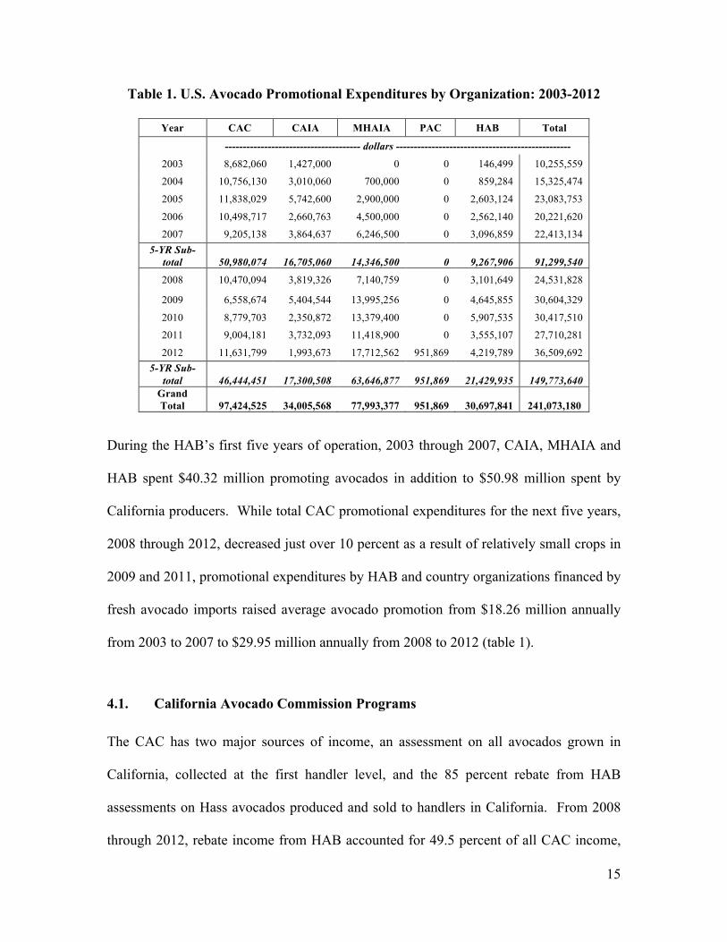
Table 1. U.S. Avocado Promotional Expenditures by Organization: 2003-2012
Year CAC CAIA MHAIA PAC HAB Total
-------------------------------------- dollars -------------------------------------------------
2003 8,682,060 1,427,000 0 0 146,499 10,255,559
2004 10,756,130 3,010,060 700,000 0 859,284 15,325,474
2005 11,838,029 5,742,600 2,900,000 0 2,603,124 23,083,753
2006 10,498,717 2,660,763 4,500,000 0 2,562,140 20,221,620
2007 9,205,138 3,864,637 6,246,500 0 3,096,859 22,413,134 5-YR Sub-
total 50,980,074 16,705,060 14,346,500
0 9,267,906 91,299,540
2008 10,470,094 3,819,326 7,140,759 0 3,101,649 24,531,828
2009 6,558,674 5,404,544 13,995,256 0 4,645,855 30,604,329
2010 8,779,703 2,350,872 13,379,400 0 5,907,535 30,417,510
2011 9,004,181 3,732,093 11,418,900 0 3,555,107 27,710,281
2012 11,631,799 1,993,673 17,712,562 951,869 4,219,789 36,509,692 5-YR Sub-
total 46,444,451 17,300,508 63,646,877
951,869 21,429,935 149,773,640 Grand Total 97,424,525 34,005,568 77,993,377
951,869 30,697,841 241,073,180
During the HAB’s first five years of operation, 2003 through 2007, CAIA, MHAIA and
HAB spent $40.32 million promoting avocados in addition to $50.98 million spent by
California producers. While total CAC promotional expenditures for the next five years,
2008 through 2012, decreased just over 10 percent as a result of relatively small crops in
2009 and 2011, promotional expenditures by HAB and country organizations financed by
fresh avocado imports raised average avocado promotion from $18.26 million annually
from 2003 to 2007 to $29.95 million annually from 2008 to 2012 (table 1).
4.1. California Avocado Commission Programs
The CAC has two major sources of income, an assessment on all avocados grown in
California, collected at the first handler level, and the 85 percent rebate from HAB
assessments on Hass avocados produced and sold to handlers in California. From 2008
through 2012, rebate income from HAB accounted for 49.5 percent of all CAC income,

16
CAC assessments accounted for 45.6 percent, and income from other sources made up
4.9 percent of all available income.
Recent CAC consumer advertising and promotion programs have focused on
California and other Western markets with messages designed to develop a premium
image for California avocados. 5 CAC focuses its marketing programs on the time period
from May through August when California fruit is now most available. During most
years radio has been the main medium for consumer advertising for CAC. An exception
was 2012 when an intensive 4th of July TV campaign was conducted in four major
California markets (Los Angeles, San Francisco, San Diego, and Sacramento).
Billboards, newspapers, cable television and the internet were also used, depending on
the market and message.
4.2. Mexican Hass Avocado Importers Association Programs
MHAIA derives about 96 percent of its operating funds from the HAB rebate. As
Mexican avocado imports have increased MHAIA has become the dominant avocado
advertising and promotion spender in the U.S. market. From 2008 through 2012,
MHAIA spent $63.65 million on advertising and promotion for avocados in the U.S.
market, accounting for 42.5 percent of producer funded programs as compared to CAC’s
31.0 percent share.
MHAIA advertising and promotion messages have reached a national audience
through magazines, a NASCAR sponsorship, The Biggest Loser television program,
5 The CAC’s core markets in 2012 included Tier 1 (Los Angeles, San Francisco, San Diego, and Sacramento); Tier 2 (Denver, Phoenix, Seattle, Portland, and Salt Lake City); Tier 3, (Austin, Dallas, San Antonio, and Houston).
17
Super Bowl and Cinco de Mayo promotions, the Big Hit Major League Baseball
promotion run during the playoffs, and spokespersons Cheryl Forberg, RD/nutritionist
and chef for NBC’s The Biggest Loser, and chef Roberto Santibañez. MHAIA also used
spot radio with retailer-specific tags and in-store demonstrations in key markets including
New York City, Chicago, Washington D.C, Boston, Baltimore, Cincinnati, Milwaukee,
Louisville, Buffalo, Rochester, Albany, Syracuse, Ithaca, St. Louis, Pittsburgh, Memphis,
Columbus, and Roanoke.
4.3. Hass Avocado Board Programs
Programs funded directly by the HAB have changed significantly over time. During its
first five years HAB had two major programs, information technology (InfoTech) and
marketing communications (MarCom) that accounted for most of its budgeted funds.
The information technology consists of the AvoHQ.com intranet and the Network
Marketing Center (NMC), designed to exchange marketing and strategic information
from all suppliers of Hass avocados to the U.S. Marketing communications consist of
consumer communications, online marketing, trade communications, industry
communications, and marketing research. The majority of HAB expenditures during its
first two years went to InfoTech. Then as InfoTech became established, funding shifted
to MarCom programs. By 2007 about 80 percent of HAB program expenditures were for
MarCom programs and about 20 percent for InfoTech.
The promotions category accounted for most of HAB’s program expenditures
during its second five years of operation (table 2). Promotions include four program
areas: consumer promotions, trade promotions, industry communications, and market and

18
nutrition research and communications. Consumer and trade promotions accounted for
just over 80 percent of total promotion expenditures in 2008, 2009, and 2010. In 2011
and 2012, HAB’s expenditures shifted from consumer and trade promotions in favor of
increased emphasis on research and communications regarding nutrition. This change
was set in motion in 2009 when HAB assumed responsibility for planning and
implementing a comprehensive avocado nutrition research program. HAB’s stated goal
was to increase awareness and improve understanding of the unique benefits of avocados
to human health and nutrition. Whereas marketing/nutrition research expenditures
accounted for 12.6 to 16.5 percent of total promotion from 2008 to 2010, such
expenditures grew to 38.4 percent of the promotion category in 2011 and further to 57.4
percent in 2012.
Table 2. HAB Expenditures by Category: 2008-2012
Year Rebates Promotion/ Market
Research
Nutrition Research
Information Admin** Total
--------------$1,000-------------- 2008* 21,991 3,005 0 590 1,676 27,262 2009 21,194 4,444 202 262 1,782 27,884 2010 24,955 5,363 544 101 1,530 32,493 2011 23,126 2,569 986 97 1,297 28,075 2012 31,879 2,104 2,115 229 1,243 37,570
*Includes 14 months of data, Nov and Dec 2007 plus calendar 2008 when HAB shifted from crop year to calendar year. ** The Program Implementation fee paid to USDA is included in the administration category.
4.4. Chilean Avocado Importers Association Programs
CAIA advertising and promotion programs are intended to increase the demand for Hass
avocados from Chile. A key strategy is to focus program resources on activities designed
to boost consumption of Hass avocados during the Chilean avocado season from

19
September through February. During the winter avocado season, most retail promotion
support is by Mexico and Chile, with Chile most active in October and November and
Mexico most active in December and January. CAIA’s total promotional expenditures
were slightly higher for 2008 through 2012 ($17.3 million) than during 2003 through
2007 ($16.7 million). However, since total Hass avocado promotion increased
substantially, CAIA’s share of expenditures dropped from 18.3 percent for 2003-2007 to
11.6 percent for the most recent five years.
CAIA’s media allocations and emphasis have varied annually as available
promotion funds changed. During 2008 and 2009 TV advertising was used in eight and
six markets, respectively, including Denver, Houston, Los Angeles, Phoenix, Portland,
San Antonio, Seattle and Rochester in 2008, and the same group minus Houston and San
Antonio in 2009. Spot radio advertising was used in another group of markets in 2008
and 2009. In 2010 most of CAIA’s promotion funds went to a joint national consumer
campaign with MHAIA and HAB. CAIA’s emphasis shifted to radio and outdoor
advertising in 2011 and, with reduced funds in 2012, to consumer-oriented outdoor
advertising in seven markets and retail promotions (in-store demos and promotions).
4.5. Peruvian Avocado Commission Programs
PAC is the newest member association, having completed its first 14 months of
operations in December 2012. PAC’s initial marketing budget included income of $1.148
million from HAB rebates and $101,222 from membership dues. Promotion activities
included public relations campaigns ($103,000), media advertising ($409,120), and trade
advertising and events ($100,000). The media activity included 200 billboards and spot

20
radio ads in six markets: Los Angeles, San Diego, Sacramento, New York/New Jersey,
Philadelphia, and Chicago. The billboards were in place for four weeks from mid-July
through mid-August, while the radio ads aired for the week of August 6, 2012.
5. Summary of Results of Prior Evaluations of Avocado Promotions
Prior to reporting the results of our analysis of promotional expenditures conducted under
the auspices of HAB for the period 2008 – 2012, we briefly summarize prior analyses of
avocado demand and evaluation of avocado promotion expenditures. Prior studies
include Carman and Green (1993), Carman and Cook (1996), Carman and Craft (1998),
and CLS (2009). On balance this work has indicated that avocado promotion programs
have induced statistically significant increases in demand. Producer returns from
advertising and promotion programs have been estimated based upon these results and
shown to have yielded attractive returns to avocado producers. For example, Carman and
Craft (1998) estimated benefit-cost ratios for avocado promotion in a range of 2.84 to
6.35. A benefit-cost ratio of 2.84 would mean that avocado producers receive an increase
of $2.84 in crop revenue for every $1.00 spent on promotion, resulting in a net return of
$1.84 for every dollar spent.
Most recently, CLS (2009) examined both annual and weekly models of U.S.
avocado demand using alternative empirical specifications in their study to gauge
effectiveness of promotional programs conducted under the auspices of HAB in its first
five years of operation. The estimated elasticity of demand of promotion expenditures
ranged from 0.15 to 0.37 in the annual models, depending upon specification. Trend
variables were included in the annual models to capture impacts on demand due to
growth in consumer incomes and changing demographics, such as growth in the Hispanic

21
share of the U.S. population. However, this same trend variable would also capture
demand growth due to changing tastes and preferences for avocados, which, in turn, are
likely due at least in part to marketing programs. Thus, the low estimate of the promotion
elasticity was viewed by CLS as a conservative lower bound on promotion’s demand
impact.
Simulation of benefit/cost ratios using the highest and lowest estimated promotion
response and price elasticities of supply of 0.50, 1.0, and 2.00 indicated that promotions
not only expanded demand for avocados but provided a positive return on funds spent.6
The estimated average and marginal benefit-cost ratios ranged from 1.12 to 6.73,
meaning that the promotional programs supported by the HAB during its first five years
(a) yielded net benefits to producers and (b) could have been profitably expanded during
the 2003-07 period of analysis. Given the range of promotion and supply elasticities used
for the simulation, CLS’s best estimate of the benefit-cost ratio for HAB promotion
programs was in the middle of the simulated range, in an interval between 2.5 and 4.0.
Analysis of avocado promotion programs in major retail markets by CLS
suggested that radio promotion significantly increased the average weekly retail sales in
promotion markets compared with non-promotion markets. Previous results also
suggested that radio is a more effective media than outdoor advertising but the difference
in effects was not statistically significant. The opportunity for CLS to conduct evaluation
6 As CLS explain in some detail, the price elasticity of supply measures the percentage response of production to a one percent increase in price. This elasticity will vary greatly for a perennial crop based upon length of run. In the short run the supply elasticity of domestic production is likely nearly zero because bearing acreage is fixed. Import supplies may, however, be more elastic because importers can shift supplies from their domestic markets or other export markets to the U.S. market in response to higher prices in the U.S.
22
based upon the available retail scanner data was limited by the industry’s inability at that
time to systematically provide disaggregate promotion expenditure information.
6. Econometric Models of the Annual Demand for Avocados
Economic theory posits that demand for a commodity is a function of that commodity’s
price, prices of goods that are used as substitutes or complements for the commodity, and
consumer income. Successful promotions can also be an important factor in expanding
demand for a product. Demographic variables such as age, ethnicity, education, and
gender may also help explain consumption of some commodities. Previous studies of
U.S. avocado demand have specified per capita consumption as a function of real prices,
per capita income, promotional expenditures, and share of Hispanic consumers. Attempts
to identify substitute or complement goods to avocados have generally been unsuccessful.
Let QA! denote per capita consumption of avocados in pounds in year t PA! the
period t average real f.o.b. farm price per pound for California avocados,7 Y! real average
per capita income for U.S. consumers, and M! the real expenditure on promotions in year
t.8 Finally, let D! represent a vector of demographic variables, such as the Hispanic
population share, that may influence demand for avocados. We can then express the U.S.
avocado demand function as
(1) QA! = f PA!,M!,Y!,D! + ε! ,
where ε! denotes a random error component.
7 Choice of variable to utilize to represent price is discussed by CLS. Ideally the price variable would be a measure of average retail prices faced by consumers in year t. Such a variable is not available. Prices throughout the market chain, however, should be closely related due simply to the workings of the market place, especially for a long time period such as a year, which gives markets full opportunities to adjust to shocks in demand and supply. Thus, movements in the annual price received by California avocado growers should closely approximate annual changes in prices observed by consumers in the U.S. 8 All monetary variables were deflated by the Consumer Price Index, base year = 1982-84.
23
The fundamental task in analyzing annual demand for fresh avocados in the U.S.
is to estimate a version of (1) econometrically. An immediate problem is that we seek to
evaluate the effectiveness of promotions conducted under the HAB’s auspices for the
five-year period from 2008 – 2012. Five observations are not nearly enough for
statistical estimation of (1). The same problem confronted CLS in their evaluation of the
Program’s first five years. They chose to estimate demand over the entire time period for
which promotion data were available, 1962-2007. This approach presented some
challenges that CLS discuss in detail, notably dealing with some structural breaks in the
demand relationships that appeared in the data between 1980 and 1981 and between 1993
and 1994.
The addition of five more years of data gives us some flexibility that CLS did not
have. We, thus, chose to focus the annual model analysis on the period 1994 – 2012, i.e.,
the period after the last structural break identified by CLS. Although this results in
considerably fewer observations than CLS analyzed, the benefit in terms of (a) avoiding
issues of structural breaks and (b) focusing the analysis on the more recent data wherein
HAB-funded promotions were in place for more than half of the observations made this
the clear choice in our view.
Another common problem in time-series analysis of demand using aggregate
annual data is that a number of variables thought to influence demand tend to move
smoothly together over time, making it difficult or impossible to isolate the effects on
demand of one such variable relative to another. CLS specifically noted this problem,
observing in particular that per capita income and the Hispanic share of the U.S.
population increased smoothly over time in a manner closely approximated by a linear

24
trend. The same issue confronts this analysis. Table 3 contains the correlation matrix for
1994 – 2012 for the key variables included in the annual model. Correlation coefficients
range from -1.0 (perfect negative correlation) to +1.0 (perfect positive correlation). A
correlation coefficient of zero denotes variables that exhibit no correlation or co-
movement. The correlation coefficient between per capita income and the U.S. Hispanic
population share is very high, 0.964. Moreover, both of these variables are highly
correlated with a simple annual trend variable, YEAR, in table 3.
The bottom line is that it is impossible with the available data to identify unique
effects of income and Hispanic population share on fresh avocado consumption.
Fortunately, these variables are only of passing interest in a study focused on promotion
effectiveness. The key consideration is to control for these factors so that they do not
introduce a bias into the estimated impact of the promotion variable. The simplest way to
do this is through including YEAR as a time-trend variable wherein it can account for
changes over time in income, Hispanic population share, and any other variables that
change over time in a smooth, linear fashion.9
Table 3. Correlation Coefficients for Demand Model: 1994-2012
Variable QAt PAt Mt Dt Yt t
Per Capita Consumption (QAt ) 1.000
Real CA Price (PAt ) -0.446 1.000
Real Total Promo Expenditures (Mt ) 0.962 -0.398 1.000
Hispanic Share of Pop. (Dt) 0.964 -0.343 0.921 1.000
Real Per Capita Dispos. Income (Yt) 0.895 -0.356 0.868 0.959 1.000
Year (t) 0.977 -0.318 0.941 0.993 0.946 1.000
9 Promotions are also quite highly correlated with per capita income, Hispanic population share, and YEAR, but there is enough independent movement in our view to identify the unique effect due to promotion expenditures.

25
Table 4 contains summary data on the key variables utilized in the annual demand
model analysis. Results of the analysis for several alternative specifications of the model
are contained in table 5.
In all cases the models in table 5 are corrected for autocorrelation in the error
term, ε!, using the Prais-Winsten procedure. Model 1 in table 5 includes real f.o.b. price,
real per capita income, and real promotion expenditures as explanatory variables. Model
2 adds a linear time trend, YEAR, to Model 1.
Table 4. Variable Definitions and Summary Statistics: 1994 – 2012 Variable Definition Units Range of
Values Mean Value
St Dev
QAt Annual average per capita U.S. sales of all avocados, (California, Florida and all imports)
pounds per capita
1.10 to 5.10
2.689 1.14
PAt Average annual f.o.b. price of California avocados deflated by the consumer price index (CPI) for all items (1982-1984=1.00)
real cents per pound
28.10 to 73.83
50.08 11.53
Yt U.S. per capita disposable income, deflated by the CPI for all items (1982-1984=1.00)
thousands of real dollars
13.24 to 16.81
15.32 1.27
Mt Annual advertising and promotion expenditures funded by HAB and CAC deflated by the CPI for all items (1982-1984=1.00)
millions of real dollars
3.44 to 15.90
8.42 4.24

26
Table 5. Annual Model Regression Results
Models 3 and 4 take account of possible endogeneity of PA! in the regression
model because f.o.b. price and consumption are determined jointly through the workings
of the market.10 Specifically these models utilize two-stage least squares estimation
wherein in stage 1, PA! is regressed on a set of instrumental variables that contribute to
explaining PA! but are not factors in explaining QA!. Following CLS, instruments chosen
for this purpose included U.S., Chilean, and Mexican avocado acreage. Fitted or
predicted values for PA! from this first-stage regression are then used in place of actual
PA! in the second-stage regression involving QA! as the dependent variable.
Real promotion expenditures represent the key variable of interest in these
models. In all cases promotion expenditures have a statistically significant and positive
impact on per capita U.S. avocado consumption. The estimated coefficients for
promotion expenditures range from 0.049 (mode1 2) to 0.113 (model 1). The two-stage
least squares models, which have the best statistical properties among the models, yield
10 See CLS for an expanded discussion of possible endogeneity problems in estimation of the annual model and solutions to the problem.
Variable Estimate t-stat Estimate t-stat Estimate t-stat Estimate t-statCalifornia FOB Price (cents/lb.) -0.012*** -3.67 -0.015*** -5.28 -0.011* -1.64 -0.001 -0.20
Per Capita Income 0.276* 1.92 -0.287*** -3.62 -0.155* -1.85
Total Promotion 0.113*** 4.18 0.049** 2.19 0.052*** 2.48 0.077** 2.93
Time Trend 0.214*** 8.17 0.180*** 6.40 0.132*** 7.46
Constant -1.633 -0.71 5.279*** 4.75 3.349** 2.33 0.754* 1.88
Durbin-Watson Statistic 1.310 1.465 - -Observations 19 19 18 18Adjusted R2 0.981 0.986 0.993 0.982
Advertising Elasticity 0.354 0.153 0.163 0.241
Model 1 (GLS) Model 2 (GLS) Model 3 (2SLS) Model 4 (2SLS)

27
intermediate values for the promotions coefficient of 0.052 and 0.077, depending upon
whether per capita income is included in the model.
Because the magnitude of the estimated coefficients depends upon the choice of
units to measure the model variables, it is desirable to convert the coefficients to
elasticities, which measure estimated percentage impacts and, thus, are unitless. The
estimated promotion elasticities evaluated at the data means range from 0.153 (model 2)
to 0.354 (model 1), a result consistent with the range of estimates reported by CLS for the
time period spanning 1962 – 2007. The differences in the estimates relates primarily to
whether the trend variable YEAR is included in the model or not. Because the promotion
variable, M!, is also collinear with YEAR, including YEAR in the model takes
“explanatory power” away from M!. As CLS noted, successful promotions are most
likely a key factor explaining the positive trend growth in per capita avocado
consumption since 1994, so the lower estimated coefficients and elasticities for the
promotion variable when YEAR is included in the model likely understate the true impact
of promotions on fresh avocado demand.
The other variables included in the model perform much as economic theory
would predict and estimates are also consistent with prior work. The f.o.b. price is
negatively related with per capita consumption in all models as predicted by the law of
demand, and the effect is statistically significant in all estimations except model 4. In the
cases where the price coefficient is statistically significant, the estimated price elasticity
of demand (evaluated at the data means) ranges from -0.205 (model 1) to -0.279 (model
2), results that are consistent with prior estimates.11
11 These price elasticity estimates are somewhat lower, however, than the range of -0.41 to -0.46 estimated by CLS. However, this difference can be explained by the rapid growth in per capita consumption in the
28
Basic economic theory would suggest that demand for fresh avocados rises as
consumers’ per capita income rises, i.e., fresh avocados are what economists call a
normal good. However, as noted, it is not possible to isolate the impact of changes in
income on avocado consumption from the other factors that are changing in consonance
with income over time. This is why the coefficient on per capita income changes from
positive to negative when YEAR is added to the model.
The trend variable YEAR itself captures the average annual increase in per capita
consumption of fresh avocados in the U.S. that is not directly accounted for by changes in
other variables in the model, notably real promotion expenditures and real price.
Depending upon the model, the estimate ranges from 0.132 pounds (model 4) to 0.214
(model 2) additional pounds per year. However, as noted, it is reasonable to assume that
some of this trend growth is in fact due to the impact of promotions, but is not reflected
in the estimated coefficient on the promotions variable.
7. Cost-Benefit Analysis of Fresh Avocado Promotion Expenditures
The econometric analysis reported in section 6 presents strong evidence that generic
promotion of fresh avocados has worked to increase the demand for fresh avocados in the
U.S. The additional question to ask, however, is whether the expenditures have “paid off”
in the sense of yielding benefits to producers from the demand enhancement that exceed
the money expended to fund the programs. We address that question in this section.
The benefit-cost analysis conducted for this study follows the methodology
utilized by CLS (2009), which is applied widely in commodity promotion evaluation presence of relatively stable prices. This means that consumers are operating in the more inelastic portions of the linear demand curves estimated in this study and supported by the data (CLS 2009).
29
studies. The average benefit-cost ratio (ABCR) from a promotion program consists of the
total incremental profit to producers generated by the program over a specified time
interval divided by the total incremental costs borne by producers to fund a program. The
ABCR is the key measure of whether a program was successful, with ABCR ≥1.0
defining a successful program.
The marginal benefit-cost ratio (MBCR) measures the incremental profit to
producers generated from a small expansion or contraction of a promotion program.
MBCR answers the question of whether expansion of the promotion program would have
increased producer profits, with MBCR > 1.0 indicating a program that could have been
profitably expanded. For the linear model utilized in this study ABCR = MBCR, and,
thus, the two questions “was the program profitable” and “could it have been profitably
expanded” are one and the same.12
Our strategy in estimating ABCR and MBCR for the promotion programs
conducted under HAB’s auspices was to simulate the impact of a small hypothetical
increase in the HAB assessment rate from the current level of $0.025/lb. to $0.03/lb., i.e.,
an increase of one-half cent per pound, and estimate the benefits and costs to avocado
growers from that assessment expansion based upon the results of the econometric
analysis discussed in the previous section.
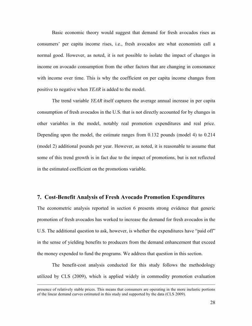
The simulation framework is depicted in figure 4, which is adapted from the CLS
study. The model begins with demand and supply functions for avocados that depict the
U.S. market for a given year t, say 2008, during the review period. Thus, demand, D!, is
total U.S. demand in t = 2008, as estimated in section 6 on a per capita basis. Supply, S!,
12 CLS conducted exhaustive statistical tests, which supported use of the linear functional form to depict demand for fresh avocados in the U.S. market.
30
is total supply to the U.S. market in t = 2008 from all sources—domestic production plus
all imports. Under the current program, total U.S. consumption in 2008, given functions
S! and D!, is Q!, and grower price is P!. Implementation of a one-half cent per pound
expansion in the program assessment increases producer costs per pound by that half
cent, which shifts supply upward to curve S!! as depicted in figure 4.
Figure 4. Avocado Promotion Simulation Model
0.5
St
Dt
A
B
C

31
The hypothetical increase in assessment generates incremental funds for
promotions equal to the change in assessment multiplied by total shipments to the U.S.
market. The marginal impact of the additional promotional expenditure on demand is
determined by the regression coefficient for the promotion variable, M!, which is reported
for alternative model specifications in table 5. The new demand curve is illustrated in
figure 4 by D!!. The new market equilibrium is found at the intersection of curves S!! and
D!! at point A in figure 4. Thus, the model predicts that equilibrium price in 2008 would
have risen to P!! and sales have risen to Q!! with the incremental assessment.
Producer benefits from the hypothetical expansion of the promotion program are
measured in terms of the change in producer surplus (PS). PS is the same as producer
variable profits, namely revenue (producer price x output) minus the variable production
costs associated with producing and selling the output. Fixed costs are irrelevant to the
calculation since they would be incurred in any event by definition of their fixity.
In figure 4, PS in the absence of the promotion program is measured by the
revenue rectangle P! ∙ Q! minus the area below the supply curve, i.e., the triangle OCQ!,
which represents the total variable costs associated with producing and selling output Q!.
We seek to measure the change, Δ, in PS associated with the hypothetical expansion of
the promotion program. In figure 4 PS after the program expansion is PS! = P!! ∙ Q!! −
0BQ!! , but we must also account for the additional promotion expenditure, which is
represented geometrically by the rectangle P!!P!!!AB = (P!! − P!!!)Q!! . Thus, the net
increase in PS to producers from expansion of the promotion program is ΔPS = PS! −
(P!! − P!!!)Q!! , which is represented by the shaded area in figure 4.

32
Information required to estimate ΔPS consists of: (i) an estimate of the marginal
impact of promotional expenditures on demand, (ii) an estimate of the slope or price
elasticity, ε!, of the grower-level demand curve, and (iii) an estimate of the slope or price
elasticity, ε!, of grower supply of avocados to the U.S. market. The results of the
econometric estimates reported in table 5 provide estimates of (i) and (ii).
Most promotion evaluation studies do not attempt to estimate the elasticity of the
supply relationship. Supply functions are difficult to estimate empirically, and the
elasticity varies by the length of run (time frame) under consideration. Any supply
relationship becomes more elastic (responsive to price) as the time horizon under
consideration expands because more productive inputs become variable to producers,
enabling them to better adjust supply to changing market signals.13
Analysis of avocado supply to the U.S. market in particular is complicated is by
the fact that both Chile and Mexico are important suppliers to the U.S. market, as well as
to their domestic markets and to other export markets. Thus, Chilean and Mexican supply
to the U.S. market is a residual supply that is based both upon total supply relationships
within each country and also domestic demand in each country and demand from all
importing countries except the U.S.14
The alternative approach utilized by CLS and by many other authors of promotion
evaluation studies is to estimate benefit-cost ratios for a range of plausible values for ε!.
The analyst then evaluates whether conclusions are robust across the range of supply
13 See Carman and Craft (1998) for detailed discussion of supply response in the California avocado industry. 14 Formally the residual supply of fresh avocados for any of the importing countries to the U.S. consists of the total supply in the country minus the domestic demand and the demands of all other importing countries. Thus, determining the price elasticity of the residual supply to the U.S. market would require estimates of the price elasticity of the total supply, as well as estimates of the price elasticity of the domestic demand and the demands of all other importing countries.

33
elasticity values chosen. If they are, then there is little need to worry about choosing
among the plausible alternative values for ε!.15
The short-run total supply of a perennial crop is highly inelastic because it is the
product of bearing acreage and yield, neither of which is likely to be influenced much by
current price. Thus, the total supply of avocados in California, Chile, Mexico, and Peru is
likely to be highly inelastic or unresponsive to current price signals. The residual supply
to the U.S. from the importing countries, however, is apt to be more elastic because the
total supply in each country can be allocated to domestic consumption or to various
export markets in response to price signals. Thus, an increase in price in the U.S. relative
to other locations due to successful promotions is likely to cause Chilean and Mexican
shippers to increase supply into the U.S. Shippers’ ability and willingness to reallocate
supply among alternative market outlets hinges on the totality of the factors discussed in
footnote 14.
CLS evaluated these considerations, and specified three alternative values, 0.5,
1.0, and 2.0, as representing a plausible range of values for ε!. The lower bound of these
values states that a one percent grower price increase in year t causes a 0.5 percent
increase in supply in year t, whereas the upper bound posits a 2.0 percent supply increase
in response to the same price signal. The five years that have ensued since CLS
conducted their analysis have seen imports’ share of the U.S. market continue to rise, as
discussed in this report, but our view is that the range of elasticities chosen by CLS
continues to represent a reasonable range of choices, and, accordingly, we adopted those
values for this analysis.
15 In addition to CLS, studies using this approach include Alston et al. (1997) for California table grapes, Alston et al. (1998) for California prunes, and Crespi and Sexton (2005) for California almonds.

34
Among the demand models included in table 5, we selected models 1 and 3 for
use in the simulation. These two models give a considerable range of values for the
impact of promotions on demand, and accommodate a range of assumptions on the
statistical properties of the demand model, most notably endogeneity or exogeneity of the
grower price.
Benefits and costs were estimated for each of the five years, 2008 – 2012, under
evaluation. The model was implemented by fitting the demand and supply functions to
the actual values observed for the real grower price and per capita consumption for each
year, thereby generating curves D! and S! intersecting at observed quantities, Q!, and
price P! in figure 4 for each year of the review period. S! was then shifted vertically to S!!
by the half cent incremental assessment for each year and D! was shifted horizontally to
D!! by the estimated promotion coefficient times the funds generated by the incremental
assessment, producing the equilibrium at point A in figure 4 and enabling us to compute
the hypothetical changes in P and Q and the ΔPS, as described in the prior paragraphs.
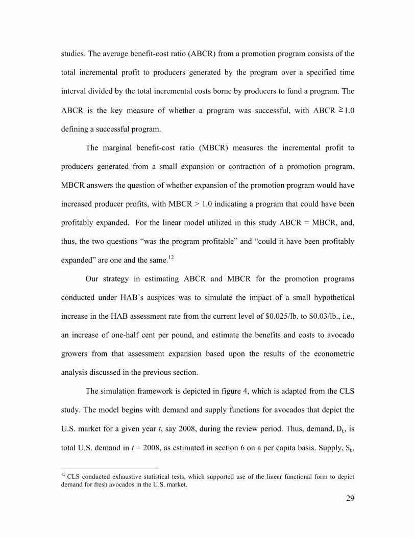
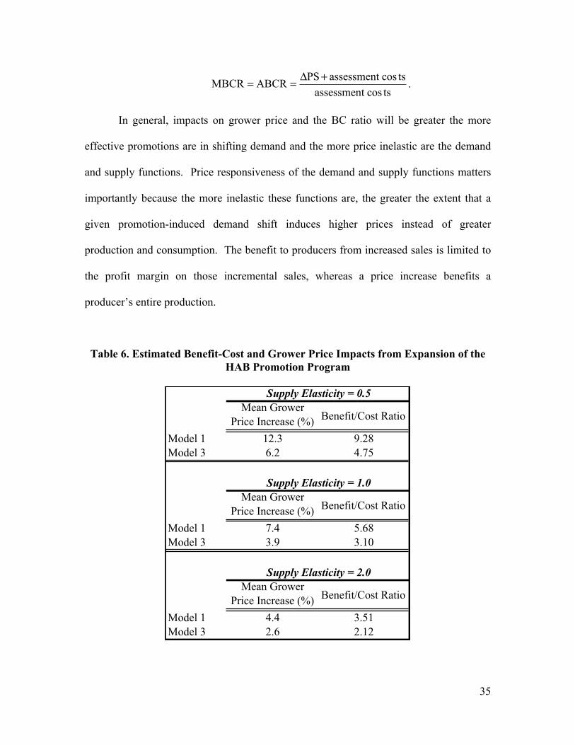
Results of the benefit-cost simulation are reported in table 6. Six sets of estimates
are reported, one for each combination of the three price elasticities of supply and two
demand models chosen for the simulation. For each simulation, table 6 reports the mean
increase in the real f.o.b. price in cents/lb. averaged over the five-year review period, and
the estimated benefit-cost (BC) ratio. Total net producer benefits are reported for each
model by compounding the annual benefits and costs over the five-year period to 2012
using a three percent real rate of interest. The BC ratio for each simulation was then
computed by adding the program cost to the estimated net benefits to produce gross
benefits and dividing gross benefits by the incremental cost:
35
MBCR = ABCR = ΔPS+ assessment cos tsassessment cos ts
.
In general, impacts on grower price and the BC ratio will be greater the more
effective promotions are in shifting demand and the more price inelastic are the demand
and supply functions. Price responsiveness of the demand and supply functions matters
importantly because the more inelastic these functions are, the greater the extent that a
given promotion-induced demand shift induces higher prices instead of greater
production and consumption. The benefit to producers from increased sales is limited to
the profit margin on those incremental sales, whereas a price increase benefits a
producer’s entire production.
Table 6. Estimated Benefit-Cost and Grower Price Impacts from Expansion of the HAB Promotion Program
Mean Grower Price Increase (%) Benefit/Cost Ratio
Model 1 12.3 9.28Model 3 6.2 4.75
Mean Grower Price Increase (%) Benefit/Cost Ratio
Model 1 7.4 5.68Model 3 3.9 3.10
Mean Grower Price Increase (%) Benefit/Cost Ratio
Model 1 4.4 3.51Model 3 2.6 2.12
Supply Elasticity = 0.5
Supply Elasticity = 1.0
Supply Elasticity = 2.0

36
The estimated BC ratios in this study range from 2.12 to 9.28. The lower bound
is associated with model 3, which has a small coefficient for promotion relative to model
1, and the most elastic supply response, ε! = 2.0. The average annual increase in the
grower price due to promotions for this simulation is 2.6 percent. The upper bound of
9.28 is associated with demand model 1, which has a high coefficient for promotion, and
with the most inelastic supply response, ε! = 0.5. The average annual price increase for
this simulation is 12.3 percent.16
The estimated BC ratios for this study in general exceed those estimated by CLS
for the Program’s first five years, which ranged from 1.12 to 6.73. The differences are
due to two effects: (i) the estimated impacts of promotions on demand are slightly higher
in this study than in CLS, and (ii) the price elasticity of demand estimated in this study is
lower than estimated by CLS. See footnote 11 for further discussion of this difference
between the two studies. As noted, a given promotion-induced shift in demand will
produce a higher benefit the more price inelastic is the demand curve.
The simulation results contained in table 6 were based upon estimated advertising
and price impacts on demand that were highly statistically significant and a plausible
range of values for the price elasticity of supply based upon economic theory. Thus, we
can conclude with a high degree of confidence that the promotional programs supported
by the HAB (i) have yielded net benefits to producers and (ii) could have been profitably
expanded.
16 The rank order of the price impacts and the BC ratios for the six simulation models is not the same. Models with inelastic demand and supply functions yield greater price impacts, other factors constant, but the more inelastic is producer supply, other factors constant, the greater the share of the incremental assessment actually borne by producers vs. shifted forward to buyers through the workings of the market. The degree to which the assessment is shifted also impacts the BC ratios.
37
To place these BC ratios in perspective, the most conservative ratio of 2.12
indicates that the 2.5 cents per pound assessment returned 5.3 cents per pound for a net
return of 2.8 cents per pound. At the upper bound, the BC ratio of 9.28 indicates that the
2.5 cents per pound assessment returned 23.2 cents per pound for a net return of 20.7
cents per pound. These, of course, are impressive rates of return, and might even strike
some observers as implausibly high. However, these rates of return are not inconsistent
with estimates derived by other authors in promotion studies conducted for other
commodities.17
In general the high rates of return found here and in a number of other studies
reflect some common features of agricultural commodity promotions. First, the
advertising intensity of these promotion programs (e.g., as measured by advertising-to-
sales ratios) is low compared to food products promoted by the leading brand
manufacturers. Promotions are subject to diminishing marginal effectiveness as the
amounts expended increase. Arguably expenditures from most commodity promotion
programs have not encountered diminishing returns due to the relatively modest amounts
collected and expended.18 Second, a characteristic of many agricultural products is that
both their demands and supplies are price inelastic. Such commodities are ideal
candidates for successful promotions because any promotion-induced demand shift will
produce a comparatively large price impact.
An additional observation in considering these results is that the findings reported
here, based upon economic and statistical analysis, confirm what is probably obvious to
17 The book by Kaiser et al. (2005) summarizes much of the prior work done on promotion evaluation with a particular focus on California commodities. 18 This argument is supported by the econometric analysis in CLS, which showed that a linear relationship between promotion expenditures and per capita consumption, implying constant returns, could not be rejected by the data.
38
most observers of the industry. Fresh avocados have gone from being a somewhat exotic,
niche product in the U.S., perhaps to be served on the occasional holiday, to a
mainstream fresh produce commodity consumed nowadays by many as a staple part of
their diets. As we have noted, many factors are involved in the remarkable growth of this
industry in the U.S., but highly successful promotion programs have surely played a
prominent role.
Finally, one should note that benefits from avocado industry growth and industry
sponsored promotional programs extend to U.S. avocado consumers, who have enjoyed
access to increased regional and seasonal availability of high quality fruit that contributes
to a healthy diet. Consumers now typically find year-round, permanent fresh avocado
displays in the retailers’ produce section containing fruit of varying maturities with “ripe
stickers” and/or instructions for determining if an avocado is ripe and how to care for it.
Retailer support and point-of-purchase promotional materials inform interested
consumers about the nutritional characteristics of avocados and provide menu
suggestions and recipes. Similar information is available on websites maintained by
HAB, CAC and the three certified importer associations. HAB’s nutrition research
programs should continue to develop information that is very useful to avocado
consumers.
8. Fresh Avocado Demand Analysis at the Retail Level
This section presents analysis of demand for fresh avocados at retail utilizing weekly
grocer scanner data aggregated to the market level. Promotional expenditures for CAC,
CAIA, and MHAIA targeted to specific regional markets in a given time period were

39
aggregated for the purposes of this analysis.19 The scanner-data analysis complements
the analysis based upon aggregate annual data and provides another vehicle to analyze
the impacts of promotions conducted under HAB’s auspices. Analysis of this
disaggregate data also enables us to make some observations about impacts of holidays
and special events and marketing strategies that may have value to the industry.
CLS also conducted similar analysis utilizing scanner data in their evaluation of
the promotions conducted under HAB’s auspices in its first five years. This analysis
differs in two important ways relative to CLS. First, CLS had access to scanner data for
individual retail chains in selected market areas, whereas the scanner data utilized here
were aggregated across chains operating within a market area by the data vendor. Second,
CAIA and MHAIA were unable to provide a breakdown of their promotional
expenditures by region and time period for the CLS study, so their analysis focused
solely on CAC expenditures. In contrast we were provided with disaggregate
expenditures for CAC, CAIA, and MHAIA, although disaggregated MHAIA data are
missing for 2008.
8.1. The Data
The data used for this analysis were collected by Information Resources, Inc. (IRI) and
supplied for this study by the Hass Avocado Board. The data include scanner data on
retail sales for fresh avocados in 38 designated marketing areas (DMA), collected on a
weekly basis for the five years spanning 2008 to 2012. Not all food retailers participate in
19 Given that there is temporal overlap in the expenditures made by the three associations, it is not possible to attribute estimated impacts to any single association’s expenditures.

40
the IRI program, so the sales reported for a DMA are not comprehensive.20 Population
data were also provided at the county level for 2010 only. Each of the DMAs is
comprised of a distinct set of counties. Thus, to obtain DMA population estimates, county
level populations were aggregated to the level of the DMA. The 2010 population data
were used to convert total DMA sales into weekly per capita sales for the entire 2008 –
2012 period. This unavoidably introduces some error into the analysis because we were
unable to account for population changes within DMAs during the study period.
Retail sales in quantity and dollar value were recorded at the price look-up (PLU)
or universal product code (UPC) level. Whereas PLU codes are specific to fruit size and
whether or not a product is organic, UPC codes are retailer specific, with some retailers
selling multiple product types and/or sizes under a single UPC. The inclusion of UPCs in
the dataset also precludes isolating sales of Hass avocados from other types of avocados.
For this reason, we aggregate all fresh avocado sales, in terms of quantity and dollar
value, in each week for each DMA. After this aggregation, a weighted average per-unit
price was calculated.
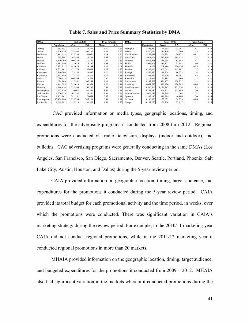
Table 7 provides population and means and standard deviations of price and sales
for each of the 38 DMAs contained in the scanner dataset. Avocado promotions were not
conducted in all 38 of these DMAs. Further, local and regional promotions were
conducted in some metropolitan areas not contained within the IRI data. Table 8
compares DMA coverage in the dataset to the metropolitan areas that received targeted
promotions for fresh avocados. All of the DMAs with an “X” in the Scanner Data column
in table 8 were included in the analysis of retail level demand for avocados.
20 The data vendor indicates that grocery stores are included in the coverage, but that supercenters and club stores are excluded. Small retailers that stock fresh avocados such as green grocers would also be excluded.
41
Table 7. Sales and Price Summary Statistics by DMA
CAC provided information on media types, geographic locations, timing, and
expenditures for the advertising programs it conducted from 2008 thru 2012. Regional
promotions were conducted via radio, television, displays (indoor and outdoor), and
bulletins. CAC advertising programs were generally conducting in the same DMAs (Los
Angeles, San Francisco, San Diego, Sacramento, Denver, Seattle, Portland, Phoenix, Salt
Lake City, Austin, Houston, and Dallas) during the 5-year review period.
CAIA provided information on geographic location, timing, target audience, and
expenditures for the promotions it conducted during the 5-year review period. CAIA
provided its total budget for each promotional activity and the time period, in weeks, over
which the promotions were conducted. There was significant variation in CAIA’s
marketing strategy during the review period. For example, in the 2010/11 marketing year
CAIA did not conduct regional promotions, while in the 2011/12 marketing year it
conducted regional promotions in more than 20 markets.
MHAIA provided information on the geographic location, timing, target audience,
and budgeted expenditures for the promotions it conducted from 2009 – 2012. MHAIA
also had significant variation in the markets wherein it conducted promotions during the
DMA DMAPopulation Mean S.D. Mean S.D. Population Mean S.D. Mean S.D.
Albany 425,963 51,388 11,841 1.00 0.21 Memphis 1,801,520 74,231 23,562 1.08 0.25Atlanta 6,546,126 274,808 104,296 1.25 0.22 Miami 4,340,266 134,849 71,790 1.45 0.34Baltimore 2,881,558 135,330 54,076 1.18 0.20 New England 2,159,039 164,734 50,828 0.91 0.14Boise 721,514 67,595 23,769 1.35 0.27 New York 21,015,004 787,466 285,918 1.33 0.28Boston 6,390,760 406,334 122,292 0.97 0.15 Orlando 3,612,518 136,238 82,385 1.43 0.31Buffalo 1,587,380 32,615 15,247 1.43 0.29 Philly 7,966,601 283,577 97,188 1.06 0.11Charlotte 2,933,357 147,675 88,838 1.21 0.68 Phoenix 513,472 769,496 200,626 0.85 0.19Chicago 9,751,961 472,276 157,694 1.25 0.23 Portland 3,149,015 405,045 143,197 1.17 0.29Cincinnati 2,360,306 73,153 29,937 1.10 0.21 Raleigh 2,859,950 149,704 86,273 1.14 0.53Columbus 2,365,889 78,232 28,519 1.17 0.18 Richmond 1,395,669 45,120 19,092 1.05 0.21Dallas 7,090,433 966,266 210,575 0.90 0.19 Roanoke 1,119,979 25,381 11,109 1.13 0.22Denver 4,034,999 627,861 207,849 1.24 0.28 Sacramento 4,167,523 651,427 209,377 1.13 0.22Detroit 4,945,785 212,626 90,974 1.00 0.18 San Diego 3,053,793 420,130 120,788 0.96 0.19Houston 6,184,414 1,028,500 241,112 0.89 0.19 San Francisco 6,860,566 1,136,743 371,334 1.08 0.23Indianapolis 2,793,170 116,070 47,551 1.11 0.18 Seattle 4,753,047 504,375 173,899 1.30 0.28Jacksonville 1,720,079 62,797 35,360 1.36 0.26 South Carolina 1,016,189 29,969 11,702 1.28 0.19Las Vegas 1,951,862 281,251 70,658 0.87 0.18 Spokane 1,102,140 118,904 40,896 1.20 0.26Los Angeles 17,838,186 2,535,799 745,104 0.94 0.18 St Louis 3,190,020 153,073 54,729 0.96 0.18Louisville 1,669,191 55,213 30,325 1.31 0.32 Tampa 4,287,277 151,354 77,917 1.32 0.25
Sales (,000) Price ($/unit) Sales (,000) Price ($/unit)

42
review period. In 2010 and 2011 MHAIA only conducted promotions on a national scale,
while in 2012 MHAIA conducted radio and “Wow Tour” promotions in more than 15
markets.
Table 8. DMAs Contained in Scanner Data and Where Promotions are Conducted
Because CAC, CAIA, and MHAIA all provided total or budgeted expenditures
for a given promotional activity and the time period, in weeks, over which the promotion
was conducted, it was necessary to convert these expenditures to a weekly basis to
DMA Promotions Scanner Data DMA Promotions Scanner DataAlbany X X Nashville XAtlanta X X New England XAustin X New Orleans XBaltimore X X New York X XBoise X X Orlando XBoston X X Palmdale XBuffalo X X Phoenix X XCentral Valley X Philadelphia X XCharlotte X X Pittsburg XChicago X X Portland X XCincinnati X X Providence XCleveland X Raleigh X XColumbus X X Richmond XDallas X X Riverside XDenver X X Roanoke X XDetroit X X Rochester XFort Myers X Sacramento X XGrand Rapids X Salt Lake City XGreensboro X San Antonio XHarrisburg X San Bernardino XHartford X San Diego X XHouston X X San Francisco X XIndianapolis X X San Jose XIthaca X Seattle X XJacksonville X X South Carolina XLas Vegas X Spokane XLos Angeles X X St. Louis X XLouisville X X Syracuse XMemphis X X Tampa X XMiami X X Virginia XMilwaukee X Washington DC X

43
conform with the scanner data. Thus, promotional expenditures were allocated to each
week in the dataset by dividing total promotional expenditures for each program by the
number of weeks the promotion ran.
National promotional activities cannot be disaggregated in order to isolate the
impact of these activities upon the DMAs contained in the scanner data and thus national
promotions were not included in this analysis of impacts at the retail level. Their
omission is not important in evaluating the impacts of local and regional promotions
because their impacts are accounted for through the month and year fixed effects
included in the regression model.
8.2. Model Specification
Two model frameworks were utilized to examine retail sales at the DMA level. One
model specified weekly fresh avocado retail sales within each DMA as a function of
promotional expenditures within the DMA as a continuous variable, current and lagged
prices, and control variables as follows:
(2) qa,t =α + [δ1pa,t ++δ p pa,t−s ]
+τ Ada,t +α t +αa + εa,t,
where q!,! is weekly sales per capita of fresh avocados in retail DMA a in week t
measured in cents, p!,!,p!,!!!, . . . ,p!,!!! represent contemporaneous and lagged retail
prices in DMA a in cents per pound, Ad!,! is total promotion expenditure measured in
thousands of dollars by CAC, CAIA, and MHAIA in retail market a at time t, individual
retail market fixed effects are represented by {0,1} indicator variables, α!, time-control

44
indicator variables, α!, account for fixed effects due to month and year, as well as to
indicate holidays and events thought to be associated with the consumption of fresh
avocados, 21 and ε!,! is a random error.22
A second specification follows what is known as the difference-in-difference
framework (see CLS for a detailed discussion) and examines the impact of presence or
absence of a promotion program in a DMA at a given time period without regard to the
magnitude of expenditure in the DMA, i.e., the presence of a promotion program in DMA
a at time t (treatment period) is denoted by an indicator variable D!,! = 1, whereas the
absence of a promotion program in market a at time 𝑡! ≠ 𝑡 (control period) is denoted by
D!,!! = 0. The estimated coefficient on this indicator variable measures the strength of
the treatment effect.
8.3. Results
Results of estimating equation (2) are presented in table 9.23 Three versions of the model
are presented which differ based upon the number of lags for the retail price included in
the model. Model 1 includes only the contemporaneous price, model 2 includes the
contemporaneous price plus a one-period lag on price (i.e., price in the preceding period),
and model 3 includes two lagged prices. All three models yield very consistent results
regarding the impact of expenditures on promotions.
21 Following CLS we denoted the presence of holidays and special events in the data by introducing a {0,1} indicator variable in the week preceding the actual event to account for purchases made to be served at the time of the event. 22 Standard errors for this analysis were clustered on DMA to account for likely correlations among errors within a DMA. 23 Table 9 excludes results for the account fixed effects, which hold little interest.
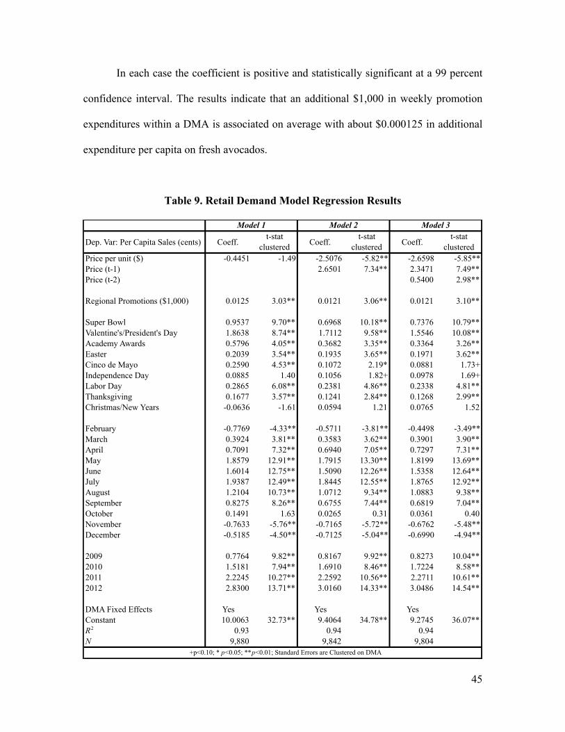
45
In each case the coefficient is positive and statistically significant at a 99 percent
confidence interval. The results indicate that an additional $1,000 in weekly promotion
expenditures within a DMA is associated on average with about $0.000125 in additional
expenditure per capita on fresh avocados.
Table 9. Retail Demand Model Regression Results
Dep. Var: Per Capita Sales (cents) Coeff.t-stat
clustered Coeff.t-stat
clustered Coeff.t-stat
clusteredPrice per unit ($) -0.4451 -1.49 -2.5076 -5.82** -2.6598 -5.85**Price (t-1) 2.6501 7.34** 2.3471 7.49**Price (t-2) 0.5400 2.98**
Regional Promotions ($1,000) 0.0125 3.03** 0.0121 3.06** 0.0121 3.10**
Super Bowl 0.9537 9.70** 0.6968 10.18** 0.7376 10.79**Valentine's/President's Day 1.8638 8.74** 1.7112 9.58** 1.5546 10.08**Academy Awards 0.5796 4.05** 0.3682 3.35** 0.3364 3.26**Easter 0.2039 3.54** 0.1935 3.65** 0.1971 3.62**Cinco de Mayo 0.2590 4.53** 0.1072 2.19* 0.0881 1.73+Independence Day 0.0885 1.40 0.1056 1.82+ 0.0978 1.69+Labor Day 0.2865 6.08** 0.2381 4.86** 0.2338 4.81**Thanksgiving 0.1677 3.57** 0.1241 2.84** 0.1268 2.99**Christmas/New Years -0.0636 -1.61 0.0594 1.21 0.0765 1.52
February -0.7769 -4.33** -0.5711 -3.81** -0.4498 -3.49**March 0.3924 3.81** 0.3583 3.62** 0.3901 3.90**April 0.7091 7.32** 0.6940 7.05** 0.7297 7.31**May 1.8579 12.91** 1.7915 13.30** 1.8199 13.69**June 1.6014 12.75** 1.5090 12.26** 1.5358 12.64**July 1.9387 12.49** 1.8445 12.55** 1.8765 12.92**August 1.2104 10.73** 1.0712 9.34** 1.0883 9.38**September 0.8275 8.26** 0.6755 7.44** 0.6819 7.04**October 0.1491 1.63 0.0265 0.31 0.0361 0.40November -0.7633 -5.76** -0.7165 -5.72** -0.6762 -5.48**December -0.5185 -4.50** -0.7125 -5.04** -0.6990 -4.94**
2009 0.7764 9.82** 0.8167 9.92** 0.8273 10.04**2010 1.5181 7.94** 1.6910 8.46** 1.7224 8.58**2011 2.2245 10.27** 2.2592 10.56** 2.2711 10.61**2012 2.8300 13.71** 3.0160 14.33** 3.0486 14.54**
DMA Fixed Effects Yes Yes YesConstant 10.0063 32.73** 9.4064 34.78** 9.2745 36.07**R2 0.93 0.94 0.94N 9,880 9,842 9,804
Model 1 Model 2 Model 3
+p<0.10; * p<0.05; **p<0.01; Standard Errors are Clustered on DMA
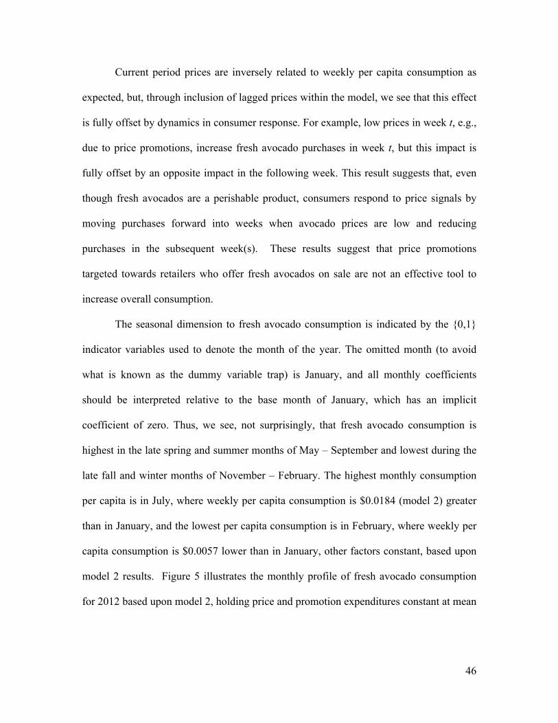
46
Current period prices are inversely related to weekly per capita consumption as
expected, but, through inclusion of lagged prices within the model, we see that this effect
is fully offset by dynamics in consumer response. For example, low prices in week t, e.g.,
due to price promotions, increase fresh avocado purchases in week t, but this impact is
fully offset by an opposite impact in the following week. This result suggests that, even
though fresh avocados are a perishable product, consumers respond to price signals by
moving purchases forward into weeks when avocado prices are low and reducing
purchases in the subsequent week(s). These results suggest that price promotions
targeted towards retailers who offer fresh avocados on sale are not an effective tool to
increase overall consumption.
The seasonal dimension to fresh avocado consumption is indicated by the {0,1}
indicator variables used to denote the month of the year. The omitted month (to avoid
what is known as the dummy variable trap) is January, and all monthly coefficients
should be interpreted relative to the base month of January, which has an implicit
coefficient of zero. Thus, we see, not surprisingly, that fresh avocado consumption is
highest in the late spring and summer months of May – September and lowest during the
late fall and winter months of November – February. The highest monthly consumption
per capita is in July, where weekly per capita consumption is $0.0184 (model 2) greater
than in January, and the lowest per capita consumption is in February, where weekly per
capita consumption is $0.0057 lower than in January, other factors constant, based upon
model 2 results. Figure 5 illustrates the monthly profile of fresh avocado consumption
for 2012 based upon model 2, holding price and promotion expenditures constant at mean
47
2012 values and setting all holiday/event and DMA market indicator variables equal to
zero.
Figure 5. 2012 Per Capita Fresh Avocado Consumption by Month
Indicator variables to denote year within the five-year review period reveal the
persistent increase in per capita consumption of fresh avocados throughout the review
period. The omitted year is 2008. Its coefficient is implicitly set to zero. We see that
weekly per capita consumption rose very consistently by from $0.006 to $0.008 per year
throughout the five-year period.24
Consistent with the results reported by CLS, we find that holidays and special
events continue to be important factors driving fresh avocado consumption. To fully
account for the impact of a holiday/event on consumption, one needs to take account both 24 For example, the indicator variable for 2009 is 0.8167 or $0.008167 in additional weekly per capita avocado consumption in 2009 compared to 2008. Weekly per capita consumption in 2012 was $0.03016 greater than 2008, or, when summed across weeks, $1.57 more than in 2008.
0"
1"
2"
3"
4"
5"
6"
Jan" Feb" Mar" Apr" May" Jun" Jul" Aug" Sep" Oct" Nov" Dec"
Es#m
ated
)Per)Cap
ita)Con
sum#o
n)(cen
ts/w
eek))(M
odel)2))
Month)

48
of the event itself and the month in which it takes place. The largest incremental impacts
in table 9 from a holiday or event are due to the Presidents’ Day/Valentine’s Day period
and the Super Bowl. However, these events occur in February, a month with very low per
capita avocado consumption apart from these special events (figure 5). Conversely,
holidays such as Cinco de Mayo and Independence Day occur during months of high
seasonal avocado consumption, so the incremental effect of these events is smaller,
although the overall avocado consumption is very high during these time periods.
Figure 6 demonstrates this point by graphing the estimated mean per capita
consumption in 2012 associated with each of the holidays/events included in table 9.
Figure 6. Per Capita Fresh Avocado Consumption During Holidays: 2012
0"
1"
2"
3"
4"
5"
6"
Super"Bowl"
Valen5ne's/President's"Day"
Academy"Awards"
Easter"
Cinco"de"Mayo"
Independence"Day"
Labor"Day"
Thanksgiving"
Christmas/New"Years"
Per$C
apita
$Con
sump/
on$(cen
ts/w
eek)$(M
odel$2)$
49
These estimates are constructed by inputting the relevant price and promotion
information for the 2012 holiday/event into the regression equation and also taking
account of the 2012 year fixed effect and the fixed effect for the month when the
holiday/event occurs. This analysis reveals that Cinco de Mayo and Independence Day
are associated with the greatest per capita consumption of fresh avocados, with,
somewhat interestingly, the Valentine’s/Presidents’ Day period having the third highest
per capita consumption, followed next by Easter.
Table 10 contains results for the difference-in-difference model wherein the
presence of local/regional promotions (aka “treatment”) at time t in DMA a is indicated
by an indicator variable, 𝐃𝐚,𝐭, set equal to 1.0, and absence of a program is denoted by
𝐃𝐚,𝐭 = 𝟎, i.e., a “control” period and location. The results from the difference-in-
difference analysis are very consistent with the results reported in table 9. The estimated
impacts of price, month, year, and holidays/events in table 10 are almost identical to what
is reported in table 9.
The presence of a local/regional promotion program in a DMA during a given
week t is associated with higher per capita sales of fresh avocados in that DMA, although
the effect is only statistically significant at the 90% confidence level for each of the three
models in table 10. The estimated impact of the presence of a promotion program in week
t in DMA a is very consistent across models—per capita sales are about $0.0026 greater
during a treatment location and time period (i.e., when a promotion is being run) than in a
control period and location when no local/regional promotions are being run.

50
Table 10. Retail Demand Model Regression Results
8.4. Discussion
Whereas the results of the aggregate annual model analysis are very conducive to the
calculation of grower benefits and costs, as was done in section 7 of this report, such
Dep. Var: Per Capita Sales (cents) Coeff.t-stat
clustered Coeff.t-stat
clustered Coeff.t-stat
clusteredPrice per unit ($) -0.4364 -1.47 -2.5021 -5.83** -2.6526 -5.86**Price (t-1) 2.6539 7.33** 2.3545 7.46**Price (t-2) 0.5338 2.94**
Regional Promotions (dummy) 0.2665 1.84+ 0.2585 1.86+ 0.2531 1.84+
Super Bowl 0.9569 9.61** 0.6998 10.06** 0.7403 10.61**Valentine's/President's Day 1.8672 8.78** 1.7142 9.62** 1.5592 10.10**Academy Awards 0.5808 4.08** 0.3690 3.35** 0.3377 3.27**Easter 0.2096 3.63** 0.1990 3.75** 0.2024 3.70**Cinco de Mayo 0.2759 4.61** 0.1235 2.41* 0.1051 1.97+Independence Day 0.1566 2.60* 0.1717 2.95** 0.1639 2.80**Labor Day 0.2874 5.96** 0.2389 4.80** 0.2347 4.75**Thanksgiving 0.1693 3.47** 0.1256 2.81** 0.1281 2.96**Christmas/New Years -0.0629 -1.64 0.0602 1.23 0.0771 1.53
February -0.7756 -4.34** -0.5693 -3.80** -0.4489 -3.46**March 0.3932 3.73** 0.3593 3.54** 0.3911 3.80**April 0.7060 7.17** 0.6913 6.90** 0.7270 7.13**May 1.8617 13.12** 1.7954 13.55** 1.8245 13.96**June 1.5983 12.83** 1.5062 12.38** 1.5342 12.87**July 1.9269 12.79** 1.8333 12.86** 1.8661 13.27**August 1.1945 10.93** 1.0558 9.43** 1.0738 9.51**September 0.8097 8.57** 0.6583 7.64** 0.6657 7.24**October 0.1399 1.54 0.0177 0.21 0.0278 0.31November -0.7717 -5.84** -0.7242 -5.82** -0.6838 -5.59**December -0.5315 -4.61** -0.7251 -5.11** -0.7109 -5.02**
2009 0.7755 9.83** 0.8160 9.97** 0.8269 10.10**2010 1.5208 7.88** 1.6940 8.39** 1.7253 8.50**2011 2.2315 10.13** 2.2661 10.40** 2.2780 10.44**2012 2.8339 13.44** 3.0203 14.13** 3.0535 14.36**
DMA Fixed Effects Yes Yes YesConstant 9.9857 32.42** 9.3850 34.05** 9.2539 35.21**R2 0.93 0.94 0.94N 9,880 9,842 9,804
Model 4 Model 5 Model 6
+p<0.10; * p<0.05; **p<0.01; Standard Errors are Clustered on DMA

51
analysis cannot be performed from the estimations based upon the disaggregate scanner
data. We were only able to estimate impacts of local/regional promotions on sales in the
grocery chains that participate with IRI. As has already been noted many food retailers do
not participate. For example, Walmart, the largest grocery retailer in the U.S. by a
considerable margin and Costco Wholesale, the third largest grocery retailer, are not in
the IRI data. Moreover, most of the media used by CAC, CAIA, and MHAIA in their
local/regional promotion campaigns extend beyond the boundaries of the target DMA,
and incremental sales of fresh avocados generated in these peripheral areas are missed
completely.
Finally, any promotion campaign is intended to have a dynamic impact on
consumption, increasing it beyond the period when the promotions are actually running.
By analyzing sales over an entire year, an annual model minimizes (but probably does
not eliminate) the problem of exclusion of dynamic impacts of promotions that spill
beyond the study period. But they are a serious problem for a weekly model such as was
studied in this section. An analyst can in principle address this problem by including
lagged values for the promotion variables. For example, an analyst who regresses q!,! on
Ad!,! and Ad!,!!! allows promotions to impact sales over two time periods. Additional
lags can be added as needed. However, that approach is not possible in this study
because we knew only the total amount expended in a DMA over a multi-week
promotion, and, thus, had no choice but to apportion the expenditure equally across those
weeks. In this case Ad!,! = Ad!,!!! and it is impossible to include both variables in the
regression model.
52
Despite these limitations, we view analysis of the weekly DMA data as providing
an important complement to and check upon the analysis of the aggregate annual data.
We were able to find a statistically significant positive impact of promotions on fresh
avocado consumption for each of the models run, as reported in tables 9 and 10. This
disaggregate analysis is not subject to the data confounds that plague analysis of annual
economic data that were discussed in detail in section 6. Thus, finding a statistically
significant and positive impact from promotion expenditures in the disaggregate data
represents an important verification of the conclusions reached based upon results from
the aggregate annual model.25
9. Conclusion
This study has evaluated the impact of promotions of fresh avocados conducted under the
auspices of the Hass Avocado Board during the second five years, 2008 – 2012, of the
Program’s existence. Our evaluation involved four central components: (i) review and
evaluation of recent trends in sales, prices, and promotions of fresh avocados in the U.S.
market (section 3); (ii) a descriptive analysis of the amounts expended and the nature of
expenditures by each of the groups participating in the program, the California Avocado
Commission, the Chilean Avocado Importers Association, the Mexican Hass Avocado
Importers Association, the Peruvian Avocado Commission, and HAB itself (section 4);
25 We also note in passing that we re-examined a question addressed by CLS concerning the issue of whether retailers adjusted price in response to targeted promotions by the industry. If retailers adjusted avocado prices upward in response to demand-increasing promotions conducted under the HAB programs, then the sales growth necessary to increase grower prices would be stifled. CLS found no evidence that retailers increased prices and, rather, found weak evidence that retailers reduced prices in response to industry promotions. We reaffirmed this conclusion based upon analysis of scanner data for the 2008 – 2012 period. It is not uncommon for food retailers to reduce prices during periods of high demand for a commodity as a way to drive traffic to the store. Observing this effect for fresh avocados means that retailer behavior, through lowering prices and featuring avocados on sale during promotion periods, complements the effects of the promotions themselves.
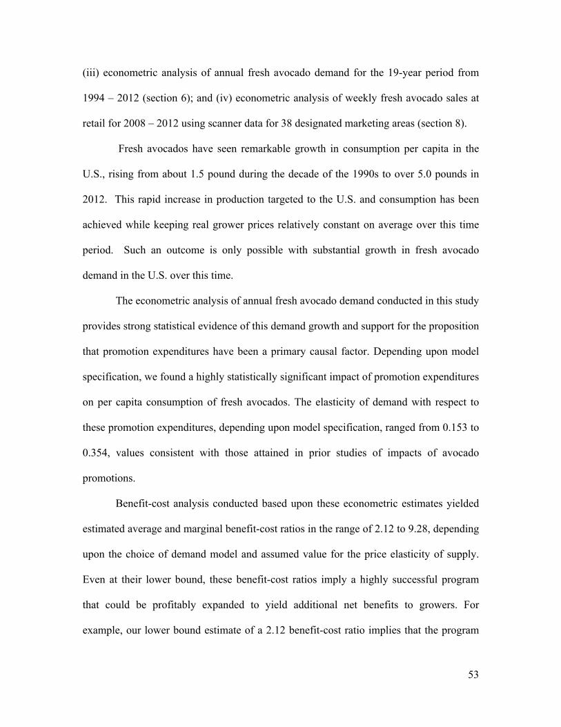
53
(iii) econometric analysis of annual fresh avocado demand for the 19-year period from
1994 – 2012 (section 6); and (iv) econometric analysis of weekly fresh avocado sales at
retail for 2008 – 2012 using scanner data for 38 designated marketing areas (section 8).
Fresh avocados have seen remarkable growth in consumption per capita in the
U.S., rising from about 1.5 pound during the decade of the 1990s to over 5.0 pounds in
2012. This rapid increase in production targeted to the U.S. and consumption has been
achieved while keeping real grower prices relatively constant on average over this time
period. Such an outcome is only possible with substantial growth in fresh avocado
demand in the U.S. over this time.
The econometric analysis of annual fresh avocado demand conducted in this study
provides strong statistical evidence of this demand growth and support for the proposition
that promotion expenditures have been a primary causal factor. Depending upon model
specification, we found a highly statistically significant impact of promotion expenditures
on per capita consumption of fresh avocados. The elasticity of demand with respect to
these promotion expenditures, depending upon model specification, ranged from 0.153 to
0.354, values consistent with those attained in prior studies of impacts of avocado
promotions.
Benefit-cost analysis conducted based upon these econometric estimates yielded
estimated average and marginal benefit-cost ratios in the range of 2.12 to 9.28, depending
upon the choice of demand model and assumed value for the price elasticity of supply.
Even at their lower bound, these benefit-cost ratios imply a highly successful program
that could be profitably expanded to yield additional net benefits to growers. For
example, our lower bound estimate of a 2.12 benefit-cost ratio implies that the program
54
returns $2.24 in incremental profit to producers for each $1.00 expended, for a net gain of
$1.24. Alternatively stated, the 2.5 cent per pound assessment yielded at least a 2.8 cent
net increase in price per pound. These estimates are somewhat higher than obtained by
Carman, Li, and Sexton (2009) in their evaluation of the HAB Program’s first five years,
but are not inconsistent with those results or with results that have been reported for other
commodity promotion programs.
Analysis of the disaggregated scanner data also found a positive and statistically
significant impact of targeted local/regional promotions on per capita sales in the targeted
marketing areas. Results from the scanner data analysis also provide important insights
for the industry as to the impacts on fresh avocado consumption of price promotions,
seasonality, and special holidays and events.
The consistency of our results across the different analyses—evaluation of trends
in avocado consumption and prices, econometric analysis of aggregate annual demand,
and econometric analysis of disaggregate weekly demand—enable us to conclude with
considerable confidence that the promotion programs conducted under the HAB’s
auspices have been successful in both expanding demand for fresh avocados in the U.S.
and yielding a very favorable return to the producers funding the program.
10. References
Alston, J.M., J.A. Chalfant, J.E. Christian, E. Meng and N.E. Piggott (1997). The California Table Grape Commission's Promotion Program: An Evaluation. Giannini Foundation Monograph no. 43, November.
Alston, J.M., H.F. Carman, J.A. Chalfant, J.M. Crespi, R.J. Sexton, and R.J. Venner
(1998). The California Prune Board's Promotion Program: An Evaluation. Giannini Foundation Research Report no. 344.
55
Bureau of Labor Statistics. Producer Price Index Detailed Reports, 2005 – 2012. http://www.bls.gov/ppi/ppi_dr.htm
California Avocado Commission. Annual Reports. Irvine, California (2002/03-2011/12).
http://commission.avocado.org/ Carman, H.F., L. Li., and R.J. Sexton (2009). “An Economic Evaluation of the Hass
Avocado Promotion Order’s First Five Years.” University of California Giannini Foundation of Agricultural Economics, Giannini Foundation Research Report 351.
Carman, H.F. and R.K. Craft (1998). “An Economic Evaluation of California Avocado
Industry Marketing Programs, 1961-1995.” Berkeley: University of California Agricultural Experiment Station, Giannini Foundation Research Report No.345, July http://giannini.ucop.edu/ResearchReports/345-Avocado.pdf.
Carman, H.F. and R.D. Green (1993). "Commodity Supply Response to a Producer
Financed Advertising Program: The California Avocado Industry." Agribusiness 9: 605-621.
Carman, H. and R. Cook (1996). “An Assessment of Potential Economic Impacts of
Mexican Avocado Imports on the California Industry.” Proceedings of the ISHS XIIIth International Symposium on Horticultural Economics. Leiden, the Netherlands: International Society for Horticultural Science (August): 227-234.
Chilean Avocado Importers Association. Annual Financial Statements (2003-12). Crespi, J.M. and R.J. Sexton (2005). “Evaluating the Effectiveness of California Almond
Promotion: How Much Did the Litigation Cost Producers?” in Kaiser, H.M., J.M. Alston, J.M. Crespi, and R.J. Sexton, eds. The Economics of Commodity Promotion Programs: Lessons from California, New York: Peter Lang Publishing, Inc., pp. 387-415.
Council of Economic Advisors, Economic Indicators, 1995-2013.
http://www.gpo.gov/fdsys/browse/collection.action?collectionCode=ECONI Hass Avocado Board. Annual Reports. Irvine, California (2008 – 2012). Kaiser, H.M., J.M. Alston, J.M. Crespi, and R.J. Sexton, eds. (2005). The Economics of
Commodity Promotion Programs: Lessons from California, New York: Peter Lang Publishing, Inc.
Mexican Hass Avocados Importers Association (MHAIA), Annual Reports, (2007 –
2012). Peruvian Avocado Commission. Financial Statements with Independent Auditors’
Report, December 31, 2012.