Fitting Linear Models DAAG Chapter 5 - Department of Statistics...

Fitting Linear Models

DAAG Chapter 5

library(DAAG)

myModel <- lm(weight ~ volume + area, data= allbacks)

summary(myModel)

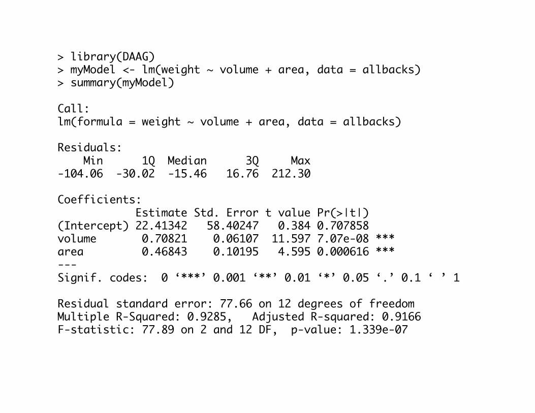
> library(DAAG)> myModel <- lm(weight ~ volume + area, data = allbacks)> summary(myModel)

Call:lm(formula = weight ~ volume + area, data = allbacks)

Residuals: Min 1Q Median 3Q Max -104.06 -30.02 -15.46 16.76 212.30

Coefficients: Estimate Std. Error t value Pr(>|t|) (Intercept) 22.41342 58.40247 0.384 0.707858 volume 0.70821 0.06107 11.597 7.07e-08 ***area 0.46843 0.10195 4.595 0.000616 ***---Signif. codes: 0 ‘***’ 0.001 ‘**’ 0.01 ‘*’ 0.05 ‘.’ 0.1 ‘ ’ 1

Residual standard error: 77.66 on 12 degrees of freedomMultiple R-Squared: 0.9285, Adjusted R-squared: 0.9166 F-statistic: 77.89 on 2 and 12 DF, p-value: 1.339e-07

> options(show.signif.stars=FALSE, digits=3)> summary(myModel)

Call:lm(formula = weight ~ volume + area, data = allbacks)


Coefficients: Estimate Std. Error t value Pr(>|t|)(Intercept) 22.4134 58.4025 0.38 0.70786volume 0.7082 0.0611 11.60 7e-08area 0.4684 0.1019 4.59 0.00062


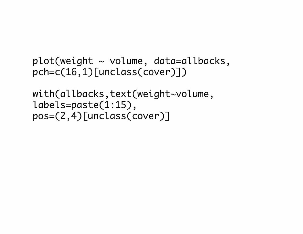
plot(weight ~ volume, data=allbacks,pch=c(16,1)[unclass(cover)])

with(allbacks,text(weight~volume,labels=paste(1:15),pos=(2,4)[unclass(cover)]

> roller weight depression1 1.9 22 3.1 13 3.3 54 4.8 55 5.3 206 6.1 207 6.4 238 7.6 109 9.8 3010 12.4 25

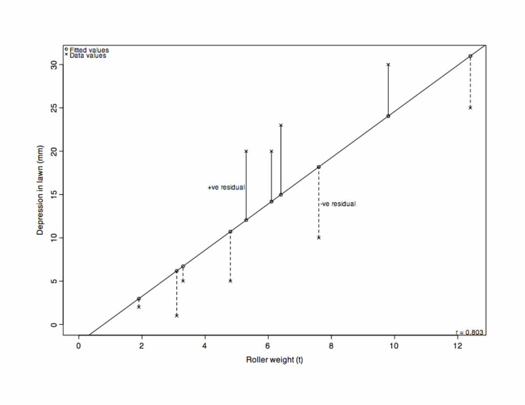
"g5.1" <-function(y = roller$depression, x = roller$weight){ oldpar <- par(mar = c(4.1, 4.1, 1.1, 1.1), mgp=c(2.5,0.75,0)) on.exit(par(oldpar)) titl <- paste("Lawn depression (mm) versus roller weight (t).", sep = "") roller.obj <- lm(y ~ x) yhat <- predict(roller.obj) ymax <- max(c(y, yhat)) plot(x, y, xlab = "Roller weight (t)", ylab = "Depression in lawn (mm)", pch = 4, xlim=c(0, max(x)), ylim=c(0, ymax)) abline(roller.obj) b <- summary(roller.obj)$coef options(digits=3) print(anova(roller.obj)) cat("\n\nCoefficients\n\n") print(b) topleft <- par()$usr[c(1, 4)]

chw <- par()$cxy[1] chh <- par()$cxy[2] legend(topleft[1], topleft[2]+0.25*chh,pch=c(1,4), legend=c("Fitted values", "Data values"), adj=0,cex=0.8, x.intersp=0.8, y.intersp=0.8, bty="n") r <- cor(x, y) bottomright <- par()$usr[c(2,3)] text(bottomright[1] - chw/2, bottomright[2]+0.5*chh, paste("r =", format(round(r, 3))), adj = 1,cex=0.8) here <- y > yhat z <- as.vector(rbind(y[here], yhat[here], rep(NA, sum(here)))) zx <- as.vector(rbind(x[here], x[here], x[here])) lines(zx, z) here <- y < yhat z <- as.vector(rbind(y[here], yhat[here], rep(NA, sum(here)))) zx <- as.vector(rbind(x[here], x[here], x[here])) lines(zx, z, lty = 2) n <- length(y) ns <- min((1:n)[y - yhat >= 0.75*max(y - yhat)]) ypos <- 0.5 * (y[ns] + yhat[ns])

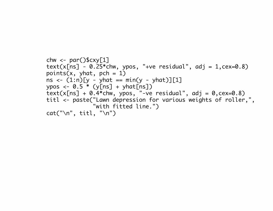
chw <- par()$cxy[1] text(x[ns] - 0.25*chw, ypos, "+ve residual", adj = 1,cex=0.8) points(x, yhat, pch = 1) ns <- (1:n)[y - yhat == min(y - yhat)][1] ypos <- 0.5 * (y[ns] + yhat[ns]) text(x[ns] + 0.4*chw, ypos, "-ve residual", adj = 0,cex=0.8) titl <- paste("Lawn depression for various weights of roller,", "with fitted line.") cat("\n", titl, "\n")

> g5.1()Analysis of Variance Table

Response: y Df Sum Sq Mean Sq F value Pr(>F)x 1 658 658 14.5 0.0052Residuals 8 363 45

Coefficients

Estimate Std. Error t value Pr(>|t|)(Intercept) -2.09 4.75 -0.439 0.67227x 2.67 0.70 3.808 0.00518

Lawn depression for various weights of roller, with fitted line. >

> sum((roller$depression-mean(roller$depression))^2)[1] 1021

> roller.lm <- lm(depression~weight, data=roller)> summary(roller.lm)

Call:lm(formula = depression ~ weight, data = roller)


Coefficients: Estimate Std. Error t value Pr(>|t|)(Intercept) -2.09 4.75 -0.44 0.6723weight 2.67 0.70 3.81 0.0052

Residual standard error: 6.74 on 8 degrees of freedomMultiple R-Squared: 0.644, Adjusted R-squared: 0.6 F-statistic: 14.5 on 1 and 8 DF, p-value: 0.00518

> plot(roller.lm,which=1)> par(mfrow=c(2,2))> plot(roller.lm,which=1:4)

residuals:

!

ˆ " i = yi # ˆ y i

plot(residuals(roller.lm)~roller$weight, ylab='Response residual', xlab='x')

plot(rstudent(roller.lm)~roller$weight, ylab='Response residual', xlab='x')

standardized residuals:

!

ˆ r i=

ˆ " i

stderr(ˆ " i)

!

stderr(ˆ " i) = ˆ # 1$ h

i

!

h = diag(X(XTX)

"1XT) leverage

Cook’s Distance

!

Di=

( ˆ " # ˆ " (i)

)T

XT

X( ˆ " # ˆ " (i)

)

dMSE

=( ˆ Y # ˆ Y

( i))

T( ˆ Y # ˆ Y

(i))

dMSE

qreference(residuals(roller.lm),nrep=8,nrows=2)

# g5.4y <- ironslag$chemicalx <- ironslag$magnetic

par(mfrow=c(2,2))

plot(x, y, xlab = "Magnetic", ylab = "Chemical", type="n")u <- lm(y ~ x)abline(u$coef[1], u$coef[2])yhat <- predict(u)lines(x, yhat)print(panel.smooth(x, y, span = 0.95, lty = 2, lwd = 1.5, pch=0))

res <- residuals(u)plot(x, res, xlab = "Magnetic", ylab = "Residual", type = "n")print(panel.smooth(x, res, span = 0.95))points(x, res, pch = 1, cex = 0.9, lwd = 1)

hat <- fitted(u)plot(hat, y, xlab = "Predicted chemical", ylab = "Chemical", type = "n")print(panel.smooth(hat, y, span = 0.95))lines(lowess(y ~ hat, f=0.9), lty=2)

yabs <- sqrt(abs(res))plot(hat, yabs, xlab = "Predicted chemical", ylab = "", type = "n")print(panel.smooth(hat, yabs, span = 0.95))

"g5.5" <-function(y = ironslag$chemical, x = ironslag$magnetic, device=""){ leg <- c("A. Residuals from fitted loess curve.", "B. Is variance about curve constant?") u <- loess(y ~ x) resval <- residuals(u) yhat <- predict(u) yabs <- sqrt(abs(resval)) plot(x, resval, xlab = "Magnetic", ylab = "Residual", pch = 1) points(x, resval, cex = 0.8, type="n") abline(h=0,lty=2) mtext(side = 3, line = 0.25, leg[1], adj = 0, cex=0.7) plot(yhat, yabs, xlab = "Predicted chemical", ylab = expression(sqrt(abs(residual))), type = "n") panel.smooth(yhat, yabs, span = 1.1, cex = 1.1)

mtext(side = 3, line = 0.25, leg[2], adj = 0, cex=0.7)}

x<-sqrt(x)plot(x,y,xlab=expression(x[2]))abline(lm(y~x))print(panel.smooth(x, y, span = 0.95, lty = 2, lwd = 1.5, pch=4))

x<-log(x)plot(x,y,xlab=expression(log(x)))abline(lm(y~x))print(panel.smooth(x, y, span = 0.95, lty = 2, lwd = 1.5, pch=0))

"g5.6" <-function(y = softbacks$weight, x = softbacks$volume, curve = c("reg"), show.fits = T, device=""){ titl <- switch(curve[1], reg = paste("Weight versus volume for softcover books,", "\nwith fitted line."), lo = paste( "Weight versus volume for softcover books,", "\nwith fitted line and S-PLUS loess smooth curve.")) u <- lm(weight ~ volume, data = softbacks) cat("\nCoefficients\n\n") options(digits=3) print(summary(u)$coef) cat("\n\n") print(anova(u)) yhat <- predict(u) r <- cor(x, y) xlim <- range(x) xlim[2] <- xlim[2]+diff(xlim)*0.08 plot(x, y, xlab = "Volume (cc)", xlim=xlim, ylab = "Weight (g)", pch = 1, ylim = range(c(y, yhat))) if(match("reg", curve, nomatch = 0)) { abline(u$coef[1], u$coef[2], lty = 1) � � z <- summary(u)$coef

if(show.fits) { points(x, yhat, pch = 1, cex = 0.75) res <- resid(u) for(i in 1:length(res)) { resi <- res[i] izzy <- as.numeric(resi > 0) xi <- x[i] yhati <- yhat[i] yi <- y[i] lines(rep(xi, 2), c(yhati, yi), col=2-izzy, lty=2-izzy) eps <- par()$cxy[1] * 0.2 if(i == 6) { adji <- 1 eps <- - eps } else adji <- 0 text(xi + eps, yhati + resi/2, paste(round(resi, 1)), adj = adji, cex = 0.65) } }} cat("\n",titl,"\n")}

"g5.6" <-function(y = softbacks$weight, x = softbacks$volume, curve = c("reg"), show.fits = T, device=""){ titl <- switch(curve[1], reg = paste("Weight versus volume for softcover books,", "\nwith fitted line."), lo = paste( "Weight versus volume for softcover books,", "\nwith fitted line and S-PLUS loess smooth curve.")) oldpar <- par(mar = c(4.1,4.1,1.1,1.1), mgp = c(2.5, 0.5, 0)) on.exit(par(oldpar)) u <- lm(weight ~ volume, data = softbacks) cat("\nCoefficients\n\n") options(digits=3) print(summary(u)$coef) cat("\n\n") print(anova(u)) yhat <- predict(u) r <- cor(x, y) xlim <- range(x) xlim[2] <- xlim[2]+diff(xlim)*0.08 plot(x, y, xlab = "Volume (cc)", xlim=xlim, ylab = "Weight (g)", pch = 1, ylim = range(c(y, yhat))) if(match("reg", curve, nomatch = 0)) { abline(u$coef[1], u$coef[2], lty = 1) z <- summary(u)$coef if(show.fits) { points(x, yhat, pch = 1, cex = 0.75) res <- resid(u) for(i in 1:length(res)) { resi <- res[i] izzy <- as.numeric(resi > 0) xi <- x[i] yhati <- yhat[i] yi <- y[i] lines(rep(xi, 2), c(yhati, yi), col=2-izzy, lty=2-izzy) eps <- par()$cxy[1] * 0.2 if(i == 6) { adji <- 1 eps <- - eps } else adji <- 0 text(xi + eps, yhati + resi/2, paste(round(resi, 1)), adj = adji, cex = 0.65) } } bottomright <- par()$usr[c(2, 3)] chw <- par()$cxy[1] chh <- par()$cxy[2] btxt <- c(paste("a =", format(round(z[1, 1], 3)), " SE =", format(round(z[1, 2], 3))), paste("b =", format(round(z[2, 1], 3)), " SE =", format(round(z[2, 2], 3)))) legend(bottomright[1], bottomright[2], legend=btxt, xjust=1, yjust=0, cex=0.8, bty="n") } cat("\n",titl,"\n")

}

softbacks.lm <- lm(weight ~ volume, data=softbacks)par(mfrow=c(2,2))plot(softbacks.lm, which=1:4)

step zero: check that the outlier is a valid data point!

M-estimators for Regression

let f denote the density for ε

let ρ = -log f

choose β to minimize:

!

"yi # xi$

s

%

& '

(

) *

i=1

n

+

MLE solves:

!

xi"yi # xi$

s

%

& '

(

) *

i=1

n

+ = 0

Can solve by IRLS with weights:

!

wi ="yi # xi$

s

%

& '

(

) *

yi # xi$

s

%

& '

(

) *

use MAD

Implementation: rlm in the MASS library

millions of phone calls in Belgium

phones.lm <- lm(calls ~ year, data=phones)plot(phones$year, phones$calls)abline(phones.lm)abline(rlm(calls~year,phones,maxiter=50), lty=2, col=2)abline(lqs(calls~year,phones), lty=3, col=3)legend(55,150,lty=1:3, col=1:3, legend=c("least squares","M-estimate","LTS"))

> summary(rlm(calls~year, maxit=50, data=phones))

Call: rlm(formula = calls ~ year, data = phones, maxit = 50)Residuals: Min 1Q Median 3Q Max -18.31 -5.95 -1.68 26.46 173.77

Coefficients: Value Std. Error t value(Intercept) -102.62 26.61 -3.86year 2.04 0.43 4.75

Residual standard error: 9.03 on 22 degrees of freedom> summary(rlm(calls~year, maxit=50, data=phones,psi=psi.bisquare))

Call: rlm(formula = calls ~ year, data = phones, maxit = 50, psi = psi.bisquare)Residuals: Min 1Q Median 3Q Max -1.658 -0.414 0.284 39.087 188.538

Coefficients: Value Std. Error t value(Intercept) -52.302 2.753 -18.999year 1.098 0.044 24.685

Residual standard error: 1.65 on 22 degrees of freedom> abline(rlm(calls~year, maxit=50, data=phones,psi=psi.bisquare),col=4)

default isHuber’s M-estimatewith c=1.345

plot(depression~weight,data=roller)roller.lm <- lm(depression~weight,data=roller)abline(roller.lm)xy <- data.frame(weight=pretty(roller$weight,20))yhat <- predict(roller.lm, newdata=xy, interval="confidence")ci <- data.frame(lower=yhat[,"lwr"],upper=yhat[,"upr"])lines(xy$weight, ci$lower, lwd=2, col="grey")lines(xy$weight, ci$upper, lwd=2, col="grey")

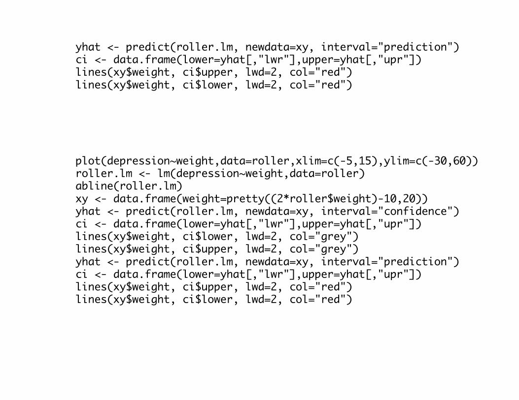
yhat <- predict(roller.lm, newdata=xy, interval="prediction")ci <- data.frame(lower=yhat[,"lwr"],upper=yhat[,"upr"])lines(xy$weight, ci$upper, lwd=2, col="red")lines(xy$weight, ci$lower, lwd=2, col="red")

plot(depression~weight,data=roller,xlim=c(-5,15),ylim=c(-30,60))roller.lm <- lm(depression~weight,data=roller)abline(roller.lm)xy <- data.frame(weight=pretty((2*roller$weight)-10,20))yhat <- predict(roller.lm, newdata=xy, interval="confidence")ci <- data.frame(lower=yhat[,"lwr"],upper=yhat[,"upr"])lines(xy$weight, ci$lower, lwd=2, col="grey")lines(xy$weight, ci$upper, lwd=2, col="grey")yhat <- predict(roller.lm, newdata=xy, interval="prediction")ci <- data.frame(lower=yhat[,"lwr"],upper=yhat[,"upr"])lines(xy$weight, ci$upper, lwd=2, col="red")lines(xy$weight, ci$lower, lwd=2, col="red")

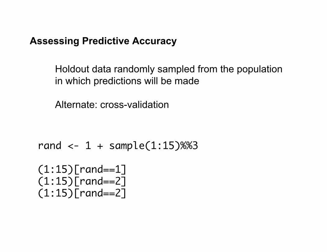
Assessing Predictive Accuracy

Holdout data randomly sampled from the population in which predictions will be made

Alternate: cross-validation

rand <- 1 + sample(1:15)%%3

(1:15)[rand==1](1:15)[rand==2](1:15)[rand==2]

houseprices.lm <- lm(sale.price ~ area, data=houseprices)CVlm(houseprices,houseprices.lm)

fold 1 Observations in test set: 3 12 13 14 15 X11 X20 X21 X22 X23x=area 802.0 696 771.0 1006.0 1191Predicted 204.0 188 199.3 234.7 262sale.price 215.0 255 260.0 293.0 375Residual 11.0 67 60.7 58.3 113

Sum of squares = 24000 Mean square = 4900 n = 5

fold 2 Observations in test set: 2 5 6 9 10 X10 X13 X14 X17 X18x=area 905 716 963.0 1018.00 887.00Predicted 255 224 264.4 273.38 252.06sale.price 215 113 185.0 276.00 260.00Residual -40 -112 -79.4 2.62 7.94

Sum of squares = 20000 Mean square = 4100 n = 5

fold 3 Observations in test set: 1 4 7 8 11 X9 X12 X15 X16 X19x=area 694.0 1366 821.00 714.0 790.00Predicted 183.2 388 221.94 189.3 212.49sale.price 192.0 274 212.00 220.0 221.50Residual 8.8 -114 -9.94 30.7 9.01

Sum of squares = 14000 Mean square = 2800 n = 5 Overall ms 3934

> summary(houseprices.lm)$sigma^2[1] 2321

> CVlm(houseprices,houseprices.lm,m=15)Overall ms 3247

Transformations

log, exp, sqrt, sqr, cube root, cube, etc.

box-cox:

!

y(")

=(y " #1) ", " $ 0

log y, " = 0

% & '

profile likelihood function for λ:

!

ˆ L (") = const #n

2log RSS(z

("))

where z(")=

y(")

˙ y "#1

geometric mean of the y’s

RSS from regression withresponse z(λ)

bc <- function(x,l) {(x^l-1)/l}l<-seq(1,4,0.5)x<-seq(-3,3,0.1)par(new=FALSE)for (i in l) {

plot(x,bc(x,i),type="l",ylim=c(-20,20),col=2*i); par(new=TRUE)}legend("top",paste(l),col=2*l,lty=rep(1,length(l)))

some details concerning the profile likelihood for Box-Cox

> attach(quine)> table(Lrn,Age,Sex,Eth), , Sex = F, Eth = A

AgeLrn F0 F1 F2 F3 AL 4 5 1 9 SL 1 10 8 0

, , Sex = M, Eth = A

AgeLrn F0 F1 F2 F3 AL 5 2 7 7 SL 3 3 4 0

, , Sex = F, Eth = N

AgeLrn F0 F1 F2 F3 AL 4 6 1 10 SL 1 11 9 0

, , Sex = M, Eth = N

AgeLrn F0 F1 F2 F3 AL 6 2 7 7 SL 3 7 3 0

y=number of days absent from school in Quine, Australia

plot(lm(Days ~ Eth*Sex*Age*Lrn, data=quine),which=1:4)

> boxcox(Days+1 ~ Eth*Sex*Age*Lrn, data = quine, lambda = seq(-0.05, 0.45, len = 20))

quineBC <- quinequineBC$Days <- (quineBC$Days^0.2 - 1)/0.2plot(lm(Days ~ Eth*Sex*Age*Lrn, data=quineBC),which=1:4)

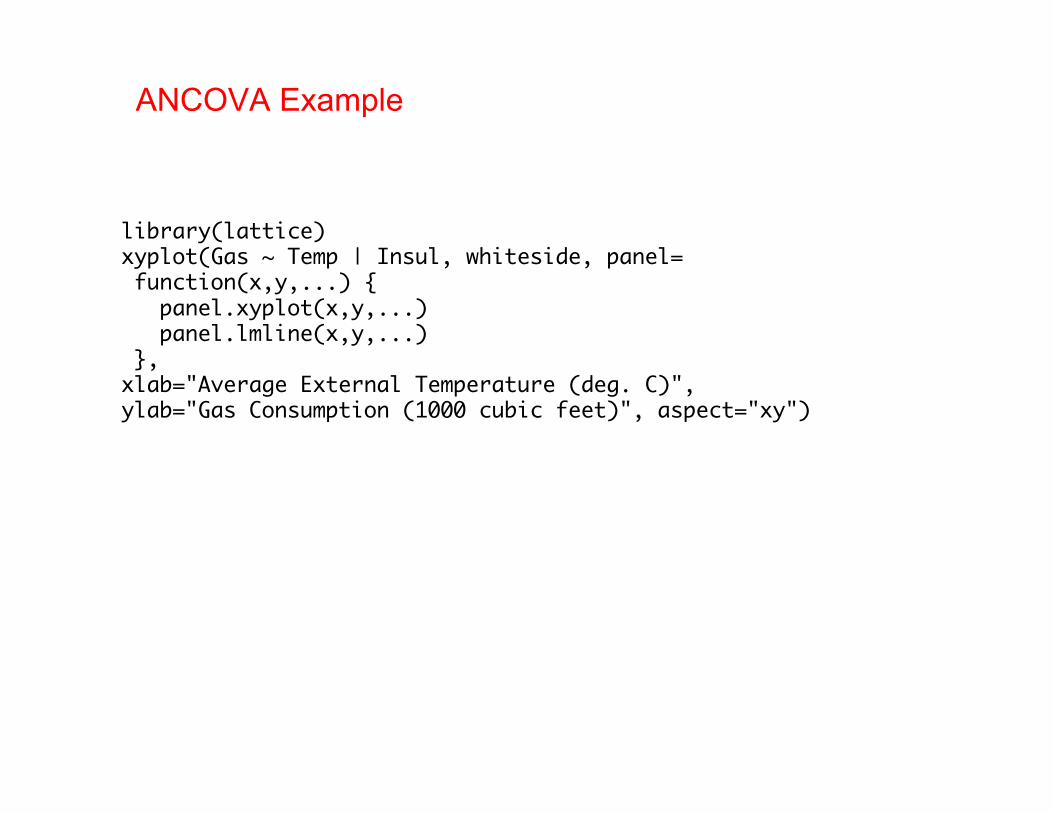
library(lattice)xyplot(Gas ~ Temp | Insul, whiteside, panel= function(x,y,...) { panel.xyplot(x,y,...) panel.lmline(x,y,...) }, xlab="Average External Temperature (deg. C)",ylab="Gas Consumption (1000 cubic feet)", aspect="xy")

ANCOVA Example

gasB <- lm(Gas ~ Temp, data=whiteside, subset=Insul=="Before")gasA <- update(gasB,subset=Insul=="After")

> summary(gasB)

Call:lm(formula = Gas ~ Temp, data = whiteside, subset = Insul == "Before")

Residuals: Min 1Q Median 3Q Max -0.62020 -0.19947 0.06068 0.16770 0.59778

Coefficients: Estimate Std. Error t value Pr(>|t|) (Intercept) 6.85383 0.11842 57.88 <2e-16 ***Temp -0.39324 0.01959 -20.08 <2e-16 ***---

Residual standard error: 0.2813 on 24 degrees of freedomMultiple R-Squared: 0.9438, Adjusted R-squared: 0.9415 F-statistic: 403.1 on 1 and 24 DF, p-value: < 2.2e-16

> summary(gasA)

Call:lm(formula = Gas ~ Temp, data = whiteside, subset = Insul == "After")


Coefficients: Estimate Std. Error t value Pr(>|t|) (Intercept) 4.72385 0.12974 36.41 < 2e-16 ***Temp -0.27793 0.02518 -11.04 1.05e-11 ***---


> summary(lm(Gas ~ Insul/Temp, data=whiteside))

Call:lm(formula = Gas ~ Insul/Temp, data = whiteside)


Coefficients: Estimate Std. Error t value Pr(>|t|) (Intercept) 6.85383 0.13596 50.41 < 2e-16 ***InsulAfter -2.12998 0.18009 -11.83 2.32e-16 ***InsulBefore:Temp -0.39324 0.02249 -17.49 < 2e-16 ***InsulAfter:Temp -0.27793 0.02292 -12.12 < 2e-16 ***---

Residual standard error: 0.323 on 52 degrees of freedomMultiple R-Squared: 0.9277, Adjusted R-squared: 0.9235 F-statistic: 222.3 on 3 and 52 DF, p-value: < 2.2e-16

fits separate Gas~Temp model for each level of Insul,but pooled estimate of variance

some evidence of curvature…

gasQ <- lm(Gas ~ Insul/(Temp + I(Temp^2)) - 1, data=whiteside)summary(gasQ)$coef Estimate Std. Error t value Pr(>|t|)InsulBefore 6.75922 0.15079 44.83 4.85e-42InsulAfter 4.49637 0.16067 27.99 3.30e-32InsulBefore:Temp -0.31766 0.06297 -5.04 6.36e-06InsulAfter:Temp -0.13790 0.07306 -1.89 6.49e-02InsulBefore:I(Temp^2) -0.00847 0.00662 -1.28 2.07e-01InsulAfter:I(Temp^2) -0.01498 0.00745 -2.01 4.97e-02

…but not much

how about a simpler model - parallel lines?

gasBA <- lm(Gas ~ Insul/Temp, data=whiteside)gasPR <- lm(Gas ~ Insul + Temp, data=whiteside)anova(gasPR, gasBA)Analysis of Variance Table

Model 1: Gas ~ Insul + TempModel 2: Gas ~ Insul/Temp Res.Df RSS Df Sum of Sq F Pr(>F) 1 53 6.77 2 52 5.43 1 1.35 12.9 0.00073 ***---

gasPR$coef(Intercept) InsulAfter Temp 6.551 -1.565 -0.337

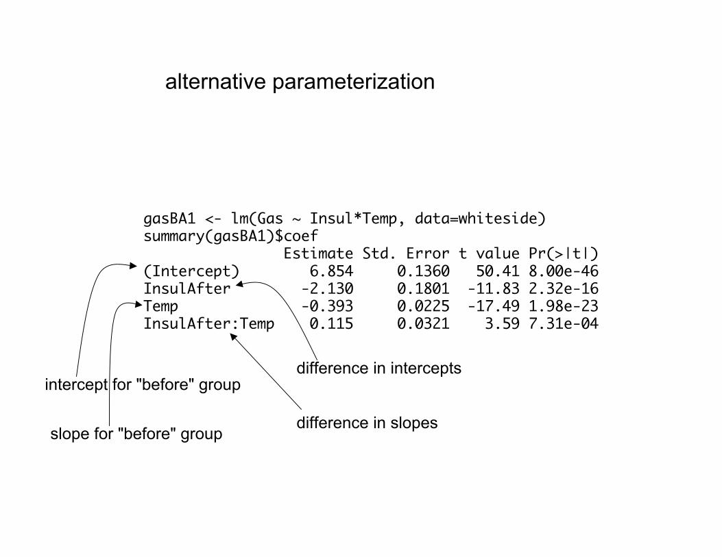
alternative parameterization

gasBA1 <- lm(Gas ~ Insul*Temp, data=whiteside)summary(gasBA1)$coef Estimate Std. Error t value Pr(>|t|)(Intercept) 6.854 0.1360 50.41 8.00e-46InsulAfter -2.130 0.1801 -11.83 2.32e-16Temp -0.393 0.0225 -17.49 1.98e-23InsulAfter:Temp 0.115 0.0321 3.59 7.31e-04

intercept for "before" groupdifference in intercepts

slope for "before" groupdifference in slopes

bootstrapping the linear model

plot(sale.price ~ area, data=houseprices)houseprices.lm <- lm (sale.price ~ area, data=houseprices)

houseprices.fn <- function(houseprices, index) { house.resample <- houseprices[index,] house.lm <- lm(sale.price ~ area, data=house.resample) abline(house.lm,lwd=0.3) coef(house.lm)[2]} houseprices.boot <- boot(houseprices, R=99, statistic=houseprices.fn)abline(houseprices.lm,col="red")

> houseprices.boot

ORDINARY NONPARAMETRIC BOOTSTRAP

Call:boot(data = houseprices, statistic = houseprices.fn, R = 99)

Bootstrap Statistics : original bias std. errort1* 0.1877769 0.01020854 0.07837381

> summary(houseprices.lm)Coefficients: Estimate Std. Error t value Pr(>|t|) (Intercept) 70.7504 60.3477 1.172 0.2621 area 0.1878 0.0664 2.828 0.0142 *

houseprices.fn <- function(houseprices, index) { house.resample <- houseprices[index,] house.lm <- lm(sale.price ~ area, data=house.resample) predict(house.lm, newdata=data.frame(area=1200))}

houseprices.boot <- boot(houseprices, R=99, statistic=houseprices.fn)

boot.ci(houseprices.boot, type="perc")

BOOTSTRAP CONFIDENCE INTERVAL CALCULATIONSBased on 99 bootstrap replicates

CALL : boot.ci(boot.out = houseprices.boot, type = "perc")

Intervals : Level Percentile 95% (247.4, 363.1 ) Calculations and Intervals on Original ScaleSome percentile intervals may be unstable

houseprices2.fn <- function(houseprices, index) { house.resample <- houseprices[index,] house.lm <- lm(sale.price ~ area, data=house.resample) houseprices$sale.price - predict(house.lm,houseprices)} R<-200houseprices2.boot <- boot(houseprices, R=R, statistic=houseprices2.fn)par(mfrow=c(1,2))n <- length(houseprices$area)house.fac <- factor(rep(1:n,rep(R,n)))plot(house.fac,as.vector(houseprices2.boot$t),ylab="Prediction Errors",xlab="House")

bootse <- apply(houseprices2.boot$t,2,sd)usualse <- predict(houseprices.lm,houseprices, se.fit=TRUE)$se.fitplot(bootse/usualse,ylab="ratio of bootse to usualse")abline(h=1)

> allbacks.lm0<-lm(weight~-1+volume+area,data=allbacks)> dfbetas(allbacks.lm0) volume area1 -0.010404410 -0.115077172 -0.001148574 -0.086585283 0.073032934 0.146651054 0.008252542 -0.016326835 -0.031975211 0.273081926 0.035027631 -0.199691057 -0.022526028 -0.033156178 -0.101903833 0.064707899 0.027442825 -0.0174259110 -0.135587040 0.0860963911 -1.309060404 0.8312399912 0.091562234 -0.0581410813 2.252231166 -1.4301438014 -0.025668104 0.0162989815 -0.164812839 0.10465447

Fitting Linear Models DAAG Chapter 5 - Department of Statistics...

Documents

Transcript of Fitting Linear Models DAAG Chapter 5 - Department of Statistics...