Fitting Data to Distributions - quantdec.com data to distributions.pdf · 3 Fitting Distributions...

Presented by Bill Huber, Quantitative Decisions, PA

Fitting Distributions to Data

Practical Issues in the Use ofProbabilistic Risk AssessmentSarasota, FloridaFebruary 28 - March 2, 1999

2

Fitting Distributions to Data, March 1, 1999

Overview

• Experiments, data, and distributions• Fitting distributions to data• Implications for PRA: managing risk

3


Objectives

By the end of this talk you should know:– exactly what a distribution is– several ways to picture a distribution– how to compare distributions– how to evaluate discrepancies that are important– how to determine whether a fitted distribution is

appropriate for a probabilistic risk analysis


Part I

Experiments, data, and distributions

5


Outcomes

• An outcome is the result of an experiment or sequence of observations.

• Examples:– The results of an opinion poll.– Data from a medical study.– Analytical results of soil samples collected for

an environmental investigation.

6


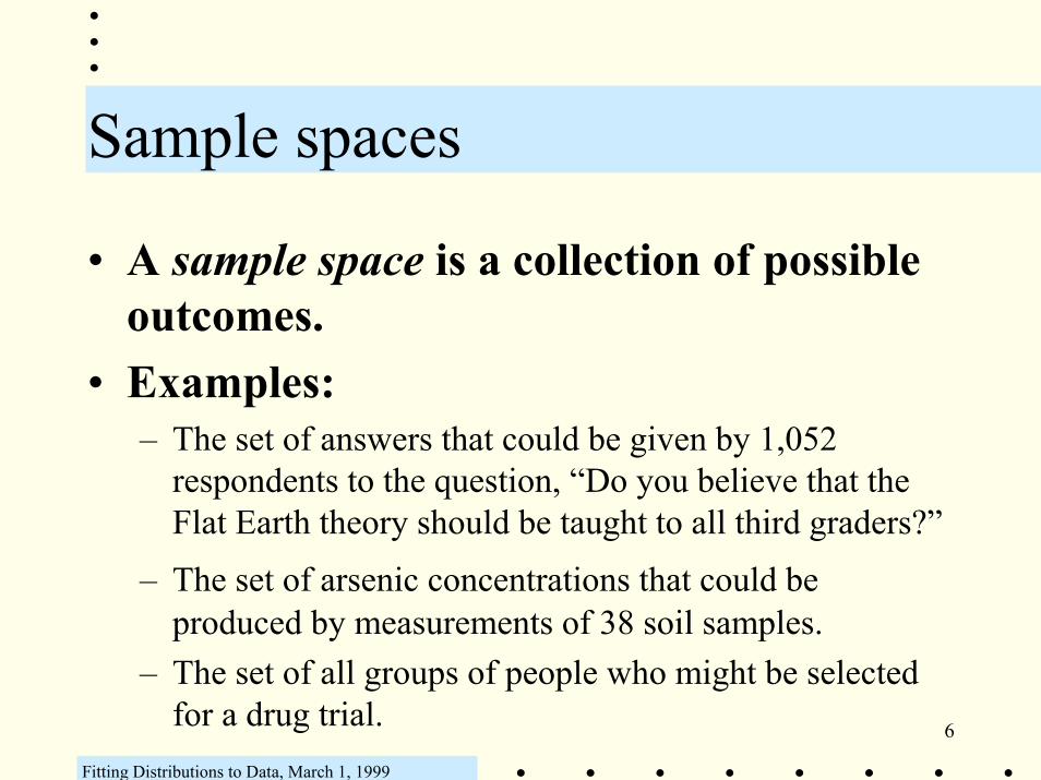
Sample spaces

• A sample space is a collection of possible outcomes.

• Examples:– The set of answers that could be given by 1,052

respondents to the question, “Do you believe that the Flat Earth theory should be taught to all third graders?”

– The set of arsenic concentrations that could beproduced by measurements of 38 soil samples.

– The set of all groups of people who might be selected for a drug trial.

7


Events

• An event is a set of possible outcomes.• Examples:

– The event that 5% of respondents answer “yes”. This event contains many outcomes because it does not specify exactly which 5% of the respondents.

– The event that the average arsenic concentration is less than 20 ppm. This event includes infinitely many outcomes.

8


Distributions

• A distribution describes the frequency or probability of possible events.

• When the outcomes can be described by numbers (such as measurements), the sample space is a set of numbers and events are formed from intervals of numbers.

9


An example

• Experiment: sample a U.S. adult at random. Measure the skin surface area.

• The sample space is the set of all surface areas for all U.S. adults.

• This set (the “population”) is constantly changing as children become adults and others die. Therefore there is no static population and there is no one distribution that is demonstrably the correct one. At best we can hope to find a succinct mathematical description that approximately agrees with the frequencies at which various skin surface areas will be observed in independent repetitions of this experiment.

10


Where data come in

• To help identify a good distribution, we samplethe present population. This means we conduct a small number of independent repetitions of the experiment. The results are the data.

• But: how do you go about finding a distribution that will describe the frequencies of futurerepetitions of the experiment?

• We will probe this issue by picturing and comparing distributions.

11


Picturing distributions: histograms

One approach is to graph the distribution’s value for a bunch of tiny equal-size non-overlapping intervals. (These are called bins.)

The values on the vertical axis are relative frequencies.

0

0 .0 2

0 .0 4

0 .0 6

0 .0 8

0 .1

0 .1 2

8

10 12 14 16 18 20 22 24 26 28 30 32 34

This is a portrait of a “squareroot normal” distribution. It

could describe natural variationin skin surface area, for example

(units are 1000 cm2).

12


Comparing distributions (1)

The histogram method, although good, has a problem: Distributions that are almost the same can look different, depending on choice of bins. Small random variations are also magnified.

0

0 .0 2

0 .0 4

0 .0 6

0 .0 8

0 .1

0 .1 2

0 .1 4

8

10 12 14 16 18 20 22 24 26 28 30 32 34 36

0

0 .0 2

0 .0 4

0 .0 6

0 .0 8

0 .1

0 .1 2

8

10 12 14 16 18 20 22 24 26 28 30 32 34

The lower distribution showsthe frequencies from 200 measure-ments of people randomly selected from the upper distribution.

13


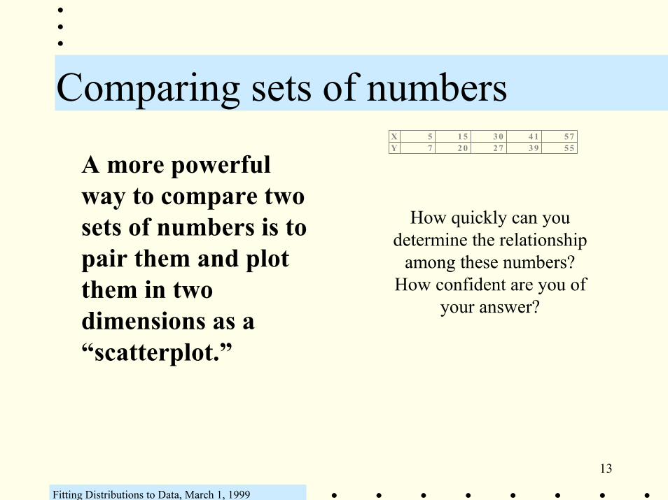
Comparing sets of numbersX 5 1 5 3 0 4 1 57Y 7 2 0 2 7 3 9 55

A more powerful way to compare two sets of numbers is to pair them and plot them in two dimensions as a “scatterplot.”

How quickly can youdetermine the relationship

among these numbers?How confident are you of

your answer?

14


Comparing sets of numbers

• The numbers are closely associated--have the same statistical “pattern”--when the scatterplot is close to a straight line.

• This approach also works nicely for comparing distributions--but first we have to find a way to pair off values in the distributions.

0

1 0

2 0

3 0

4 0

5 0

6 0

0 2 0 4 0 6 0

X 5 1 5 3 0 4 1 57Y 7 2 0 2 7 3 9 55

15


Comparing distributions (2)

• Given: one data set.• To compare its

distribution to a reference, generate the same number of values from the reference. Pair data and reference values from smallest-smallest to largest-largest, as illustrated.

Order Percentile Reference Measured1 0.25% - 2.81 10.02 0.75% - 2.43 10.83 1.25% - 2.24 11.04 1.75% - 2.11 11.2

197 98.25% 2.11 29.9198 98.75% 2.24 30.3199 99.25% 2.43 34.2200 99.75% 2.81 35.3

. . .

0

0 . 0 2

0 . 0 4

0 . 0 6

0 . 0 8

0 .1

0 . 1 2

0 . 1 4

8

10 12 14 16 18 20 22 24 26 28 30 32 34 36

0

0 .0 2

0 .0 4

0 .0 6

0 .0 8

0 .1

0 .1 2

8

10 12 14 16 18 20 22 24 26 28 30 32 34

Reference Measured

16


Probability plots

10

15

20

25

30

35

40

-3 -2 -1 0 1 2 3Expected value for standard normal distribution

Finally, draw the scatterplot. It is close to a straight line: the data and its reference distribution therefore have the same shape (although one might be shifted and rescaled relative to the other).

This is a probability plot.

17


Reading probability plots

10

15

20

25

30

35

40

pp

-3 -2 -1 0 1 2 3Expected value for standard normal distribution

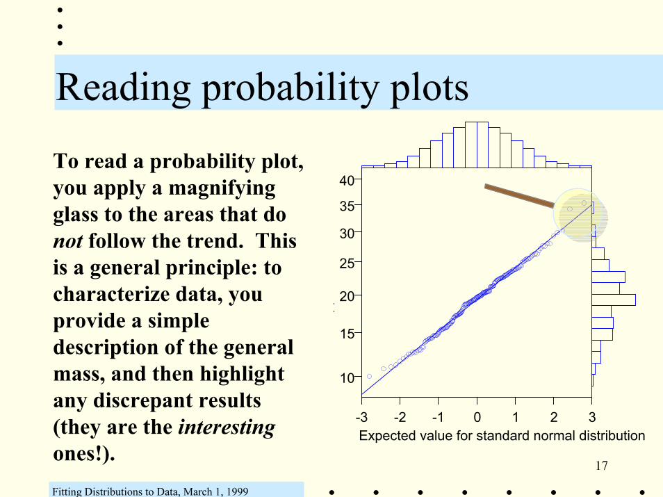
To read a probability plot, you apply a magnifying glass to the areas that do not follow the trend. This is a general principle: to characterize data, you provide a simple description of the general mass, and then highlight any discrepant results (they are the interestingones!).

18


Statistical magnification

The two largest points are slightly higher than the line.

Interpretation: our largest measurements have a slight tendency to be larger than the largest measurements in the reference distribution. (The amount by which they are larger is inconsequential, though.)

19


Interpretation issues

• What do we use for a reference distribution? Why?

• Which deviations from the reference should concern us?

• How much of a deviation is important?• What risk do we run if a mistake is made

in the interpretation?All these questions are interrelated.

20


Progress update

• We have a scientific framework and language for discussing measurements and observations, events and distributions.

• You have learned to picture distributions using histograms.

• You have learned to compare (and depict) distributions using probability plots.

• You have learned to use statistical magnification to evaluate deviations from a reference standard.

0

0 .0 2

0 .0 4

0 .0 6

0 .0 8

0 .1

0 .1 2

0 .1 4

8

10 12 14 16 18 20 22 24 26 28 30 32 34 36

10

15

20

25

30

35

40

As,

ppm

, as

mea

sure

d

-3 -2 -1 0 1 2 3Expected value for standard normal dis


Part II

Fitting distributions to data

22


An example data setAs, ppm

3.9 32.9 68.9 116.05.2 32.9 68.9 116.06.0 36.0 78.4 117.57.5 37.6 79.9 150.49.9 43.9 84.6 172.4

10.7 45.4 89.3 219.415.7 45.4 89.3 220.921.9 50.1 94.0 222.525.1 51.7 111.3 264.831.3 112.8

• Let’s take a close look at some arsenic measurements of soil samples.

• What is the first thing you would do with these data?

23


The first thing to do

• Ask why.• If you don’t know how the data will be

used to make a decision or take an action, then any analysis you attempt is likely to be misleading or irrelevant.

Do not be tempted to embark on an analysis of data simply because they are there and you have some tools to do it with.

24


The purpose and its implications

In our example, the arsenic measurements will be used to develop a concentration term for a human health risk assessment.

Therefore:– We want to characterize the arithmetic mean

concentration– We do not want to grossly underestimate the mean– We should focus on characterizing the largest

values best.

25


The second thing to do

0 100 200 300AS

0

4

8

12

Cou

n t

0.0

0.1

0.2

0.3

0.4

Proportion per Bar

Draw a picture.

As, ppm

3.9 32.9 68.9 116.05.2 32.9 68.9 116.06.0 36.0 78.4 117.57.5 37.6 79.9 150.49.9 43.9 84.6 172.4

10.7 45.4 89.3 219.415.7 45.4 89.3 220.921.9 50.1 94.0 222.525.1 51.7 111.3 264.831.3 112.8

26


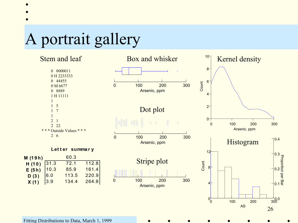
A portrait gallery

0 00000110 H 22333330 444550 M 66770 88891 H 1111111 51 712 12 22

* * * Outside Values * * *2 6

Stem and leaf

0 100 200 300Arsenic, ppm

Box and whisker


Dot plot


Stripe plot


0

2

4

6

8

10

Cou

n t

Kernel density

0 100 200 300AS

0

4

8

12

Cou

nt0.0

0.1

0.2

0.3

0.4

Proportion per Bar

HistogramLet t er summa r y

M (1 9 h) 60.3H (1 0 ) 31.3 72.1 112.8E (5 h) 10.3 85.9 161.4D (3 ) 6.0 113.5 220.9X (1 ) 3.9 134.4 264.8

27


The third thing to do: compare

0

100

200

300

AS0 1 2 3 4 5

Expected Value for Exponential Distribution

0

100

200

300

AS

0 1 2 3 4 5 6 7Expected Value for Gamma(2) Distribution

1

2

4

8

16

32

64

128

256

0.0 0.1 0.2 0.3 0.4 0.5 0.6 0.7 0.8 0.9 1.0Expected Value for Uniform Distribution

60

120

180

240

300

AS

-3 -2 -1 0 1 2 3Expected Value for Normal Distribution

0

100

200

300

AS

0.0 0.1 0.2 0.3 0.4 0.5 0.6Expected Value for Beta(1,5) Distribution

0

100

200

300

AS0 2 4 6 8 10 12Expected Value for Chi-square(3) Distribution

28


Shades of “normal”Normal Cube root normal Lognormal

60

120

180

240300

AS


0

100

200

300

AS


2

4

8

163264

128256512

AS


The middle fits the best. It is neither normal nor lognormal.--But none fit as well as some of the previous distributions.

29


A closer look at a good fit

• The fit to the upper 75% of data--the large ones, the ones that really count--is beautiful.

• Yet, the uniform distribution has lower and upper limits. Do you really think the arsenic concentrations at a site would be so definitely limited?

2

4

8

16

32

64

128

256

512

Arse

nic,

pp m

(log

sca

l e)


30


A key point, repeated

• Keep asking, “what effect could a (potential) characterization of the data have on the decision or action?”

• If we describe the example data in terms of a log-uniform distribution, then we have decided to treat them as having an upper bound (of about 300 ppm) and are therefore implicitly not considering the possibility there may be much higher concentrations present. This is usually not a good assumption to make when few measurements are available.

31


What the many comparisons show

• The question is not “what is the best fit?” (So don’t go on a distribution hunt!)

• The issue is to select a reference distribution that– Fits the data well enough– Has a basis in theory or empirical experience– Manages the risk attached to using the

reference distribution for further analysis and decision making.

32


Measuring fits “well enough”

- 1.0

- 0.5

0.0

0.5

1.0

1.5

2.0

2.5

3.0

0.00 10.00 20.00 30.00 40.00

Theor et ica l f it

Mea

sure

d Va

lue

• Recall that “statistical magnification” explores the differences between the data and the reference distribution. These differences can be graphed.

33


What it means to fit “well enough” Statistical theory provides

– Methods to measure these differences

– Methods to determine the chance that such differences are just random deviations from the reference distribution:

• Kolmogorov-Smirnov• Anderson-Darling• Shapiro-Wilks

However, do not become a slave to the P-value: it’s a measurement, not a rule.

P = 20.3428864%

- 1.0

- 0.5

0.0

0.5

1.0

1.5

2.0

2.5

3.0

0.00 10.00 20.00 30.00 40.00

Theor et ica l f it

Mea

sure

d Va

lue

34


The role of theory and experience• Observations or measurements may vary for many

reasons, including– Accumulated independent random “errors” not controlled by the

experimenter– Natural variation in the population sampled.

• The form of variation can also depend on– Mechanism of sample selection or observation: random, stratified,

focused, etc.– What is being observed: representative objects, extreme objects

(such as floods), etc.

• Both theory and experience often suggest a form for the reference distribution in these cases.

35


Examples of reference distributions

• Normal distribution: variation arises from independent additive “errors.”

• Lognormal: variation arises from independent multiplicative errors. Often observed in concentrations of substances in the environment. (Often confused with mixtures of normal distributions, too!)

• Many other well known mathematical distributions describe extreme events, waiting times between random events, etc.


Part III

Managing Risk

37


Managing risk• Begin by considering how discrepancies between reality

and the model might affect the decision.• Example: Concentration of pollutant due to direct

deposition onto plant surfaces is estimated as

Pd = [Dyd + (Fw * Dyw)] * Rp * [1 - exp(-kp * Tp)]Yp * kp

Dyd = yearly dry deposition rate, Dyw = wet rate, Fw = adhering fraction of wet deposition, Rp = interception fraction of edible portion, kp = plant surface loss coefficient, Tp = time of plant’s exposure to deposition, Yp = yield

(USEPA 1990: Methodology for Assessing Health Risks Associated WithIndirect Exposure to Combustor Emissions).

A large value of a red (italic) variable or a small value of a bluevariable creates a large value of Pd.

38


Managing risk, continued Pd = [Dyd + (Fw * Dyw)] * Rp * [1 - exp(-kp * Tp)]

Yp * kp A large value of a red variable or a small value of a blue variable

creates a large value of Pd. Suppose:

– These variables are modeled as distributions in a probabilistic risk assessment

– The decision will be influenced by the large values of Pd (pollutant concentration potentially ingested by people).

Then, look at the important tail:– Make sure the upper tail fits the data for a red variable well– Make sure the lower tail fits the data for a blue variable well.

39


Managing risk: examplesA large value of a red variable or a small value of a blue variable creates a large value of Pd.

1

2

4

8

16

32

64

128

256


60

120

180

240

300

AS


2

4

8

16

3264

128256512

AS-3 -2 -1 0 1 2 3

Expected Value for Normal Distribution

On the left, a blue variable: the reference distribution (straight line) underestimates the data values; therefore using the reference distribution in a PRA may overestimate the pollutant concentration. Now you evaluate the middle and right pictures for a blue and red variable, respectively.

40


Evaluation Checklist

• A defensible choice of distribution simultaneously:– Can be effectively incorporated in subsequent analyses; is

mathematically or computationally tractable– Fits the data well at the important tail– Has a scientific, theoretical, or empirical rationale.

• Red flags (any of which is cause for scepticism):– A distribution was fit from a very large family of possible

distributions using an automated computer procedure– The distribution was never pictured– The distribution is unusual and has no scientific rationale– The important tail of the distribution deviates from the data in an

anti-conservative way.

41


Conclusion

You should now know– exactly what a distribution is– several ways to picture a distribution– how to compare distributions– how to evaluate discrepancies that are important– how to determine whether a fitted distribution is

appropriate for a probabilistic risk analysis.

Fitting Data to Distributions - quantdec.com data to distributions.pdf · 3 Fitting Distributions...

Documents

Transcript of Fitting Data to Distributions - quantdec.com data to distributions.pdf · 3 Fitting Distributions...