Fitting Bivariate Models October 21, 2014 Elizabeth Prom-Wormley & Hermine Maes [email protected]...

Fitting Bivariate Models

October 21, 2014

Elizabeth Prom-Wormley & Hermine Maes

[email protected]

804-828-8154

The Problem(s)

• BMI may not be an appropriate measure for use in studying the genetics of obesity– Do height and weight share the same

genetic/environmental influences?

• Smoking is a risk factor for cardiovascular disease, but how ?– Does smoking in adolescence lead to

cardiovascular disease in adulthood?

A SolutionBivariate Genetic Analysis

• Two or more traits can be correlated because they share common genes or common environmental influences– e.g. Are the same genetic/environmental

factors influencing the traits?

• With twin data on multiple traits it is possible to partition the covariation into its genetic and environmental components– Goal: to understand what factors make sets of

variables correlate or co-vary

Bivariate AnalysisA Roadmap

1- Use the data to test basic assumptions inherent to standard genetic models

Saturated Bivariate Model

2- Estimate the contributions of genetic and environmental factors to the covariance between two traits

Bivariate Genetic Models (Bivariate Genetic Analysis via Cholesky Decomposition)

Getting a Feel for the DataPhenotypic and Twin Correlations

MZ DZ

Height

2Weight

2 Height

2Weight

2Height1 0.88 0.41 0.44 0.23Weight1 0.49 0.84 0.17 0.33

Open R script for today

rWeight/Height = 0.47

Getting a Feel for the DataPhenotypic and Twin Correlations

MZ DZ

Height

2Weight

2 Height

2Weight

2Height1 0.88 0.41 0.44 0.23Weight1 0.49 0.84 0.17 0.33

rWeight/Height = 0.47

Expectations1- rMZ > rDZ (cross-twin/cross-trait)Genetic effects contribute to the relationship between height and weight

2- Cross-twin cross-variable correlations are not as big as the correlations between twins within variables. Variable specific genetic effects on height and/or weight

So…How Can We be Sure?

Building the Bivariate Genetic ModelSources of Information

• Cross-trait covariance within individuals– Within-Twin Covariance

• Cross-trait covariance between twins– Cross-Twin Covariance

• MZ:DZ ratio of cross-trait covariance between twins

Basic Data Assumptions

• MZ and DZ twins are sampled from the same population, therefore we expect – Equal means/variances in Twin 1 and Twin 2– Equal means/variances in MZ and DZ twins– Equal covariances between Twin 1 and Twin

2 in MZ and DZ twins

9

Getting a Feel for the DataMeans

ht1 wt1 ht2 wt2

MZ 16.30 5.67 16.29 5.65

DZ 16.41 5.82 16.33 5.77

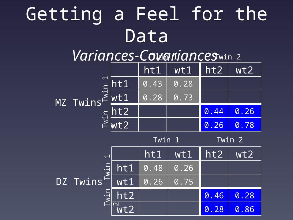
Getting a Feel for the DataVariances-Covariances

ht1 wt1 ht2 wt2ht1wt1ht2wt2

ht1 wt1 ht2 wt2ht1wt1ht2wt2

MZ Twins

DZ Twins

Twin 1 Twin 2

Twin

1Tw

in

2

Twin 1 Twin 2

Twin

1Tw

in

2


Variances

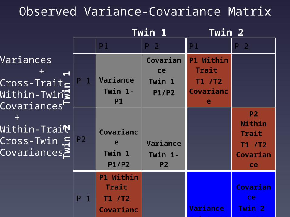
Observed Variance-Covariance Matrix

P1 P 2 P1 P 2

P 1Variance Twin 1-

P1

P2Variance Twin 1-

P2

P 1 Variance Twin2- P1

P 2Variance Twin 2-

P2

Twin 1 Twin 2

Twin

1Tw

in 2

Variances


ht1 wt1 ht2 wt2ht1 0.43

wt1 0.73

ht2 0.44

wt2 0.78

ht1 wt1 ht2 wt2ht1 0.48

wt1 0.75

ht2 0.46

wt2 0.86

MZ Twins

DZ Twins

Twin 1 Twin 2

Twin

1Tw

in

2

Twin 1 Twin 2

Twin

1Tw

in

2


Cross-Trait / Within-Twin

Covariance


P1 P 2 P1 P 2

P 1 Variance Twin 1- P1

Covariance

Twin 1 P1/P2

P2

Covariance

Twin 1 P1/P2

Variance Twin 1- P2

P 1 Variance Twin2- P1

Covariance

Twin 2 P1/P2

P 2

Covariance

Twin 2 P1/P2

Variance Twin 2- P2

Twin 1 Twin 2

Twin

1Tw

in 2

Variances+

Cross-TraitWithin-TwinCovariances


ht1 wt1 ht2 wt2ht1 0.43 0.28

wt1 0.28 0.73

ht2 0.44 0.26

wt2 0.26 0.78

ht1 wt1 ht2 wt2ht1 0.48 0.26

wt1 0.26 0.75

ht2 0.46 0.28

wt2 0.28 0.86

MZ Twins

DZ Twins

Twin 1 Twin 2

Twin

1Tw

in

2

Twin 1 Twin 2

Twin

1Tw

in

2


Cross-Trait / Within-Twin

Covariance


P1 P 2 P1 P 2

P 1 Variance Twin 1- P1

Covariance

Twin 1 P1/P2

P1 Within Trait T1 /T2

Covariance

P2 Covariance Twin 1 P1/P2

Variance Twin 1- P2


Covariance

P 1

P1 Within Trait

T1 /T2 Covariance

Variance Twin2- P1

Covariance

Twin 2 P1/P2

P 2

P2 Within Trait

T1 /T2 Covarianc

e

Covariance Twin 2 P1/P2

Variance Twin 2- P2

Twin 1 Twin 2

Twin

1Tw

in 2

Variances+


+Within-TraitCross-Twin Covariances


ht1 wt1 ht2 wt2ht1 0.43 0.28 0.38

wt1 0.28 0.73 0.64

ht2 0.38 0.44 0.26

wt2 0.64 0.26 0.78

ht1 wt1 ht2 wt2ht1 0.48 0.26 0.21

wt1 0.26 0.75 0.27

ht2 0.21 0.46 0.28

wt2 0.27 0.28 0.86

MZ Twins

DZ Twins

Twin 1 Twin 2

Twin

1Tw

in

2

Twin 1 Twin 2

Twin

1Tw

in

2


Cross-Trait / Cross-Twin Covariance


P1 P 2 P1 P 2

P 1Variance Twin 1- P1

Covariance

Twin 1 P1/P2


Covariance

P1/P2 Cross-Trait

T1 /T2 Covarianc

e


Variance Twin 1- P2

P2/P1Cross-Trait

T1 /T2 Covariance


Covariance

P 1P1 Within

Trait T1 /T2

Covariance

P2/P1Cross-Trait

T1 /T2 Covarianc

eVariance Twin2- P1

Covariance

Twin 2 P1/P2

P 2

P1/P2 Cross-Trait

T1 /T2 Covariance

P2 Within Trait

T1 /T2 Covarianc

e


Variance Twin 2- P2

Twin 1 Twin 2

Twin

1Tw

in 2

Variances+




P1 P 2 P1 P 2

P 1Variance Twin 1- P1

Covariance

Twin 1 P1/P2


Covariance

P1/P2 Cross-Trait

T1 /T2 Covarianc

e


Variance Twin 1- P2

P2/P1Cross-Trait

T1 /T2 Covariance


Covariance

P 1P1 Within

Trait T1 /T2

Covariance

P2/P1Cross-Trait

T1 /T2 Covarianc

eVariance Twin2- P1

Covariance

Twin 2 P1/P2

P 2

P1/P2 Cross-Trait

T1 /T2 Covariance

P2 Within Trait

T1 /T2 Covarianc

e


Variance Twin 2- P2

Twin 1 Twin 2

Twin

1Tw

in 2

Variances+



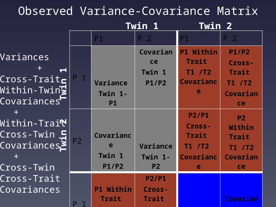
+Cross-TwinCross-TraitCovariances


P1 P 2 P1 P 2

P 1Variance

P1

P2 Covariance P1-P2

Variance P2

P 1Within-

traitP1

Cross-trait Variance

P1

P 2 Cross-traitWithin-

traitP2

Covariance P1-P2

Variance P2

Twin 1 Twin 2

Twin

1Tw

in 2

Within-twin covariance

Within-twin covariance

Cross-twin covariance


ht1 wt1 ht2 wt2ht1 0.43 0.28 0.38 0.24

wt1 0.28 0.73 0.28 0.64

ht2 0.38 0.28 0.44 0.26

wt2 0.24 0.64 0.26 0.78

ht1 wt1 ht2 wt2ht1 0.48 0.26 0.21 0.15

wt1 0.26 0.75 0.11 0.27

ht2 0.21 0.11 0.46 0.28

wt2 0.15 0.27 0.28 0.86

MZ Twins

DZ Twins

Twin 1 Twin 2

Twin

1Tw

in

2

Twin 1 Twin 2

Twin

1Tw

in

2

• Within-twin cross-trait covariances imply common etiological influences

• Cross-twin cross-trait covariances imply familial common etiological influences

• MZ/DZ ratio of cross-twin cross-trait covariances reflects whether common etiological influences are genetic or environmental

Cross-Trait Covariances

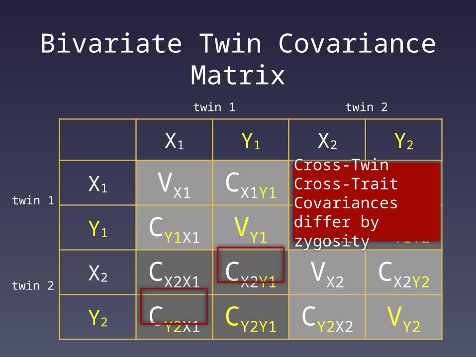
Bivariate Twin Covariance Matrix

X1 Y1 X2 Y2

X1 VX1 CX1Y1 CX1X2 CX1Y2

Y1 CY1X1 VY1 CY1X2 CY1Y2

X2 CX2X1 CX2Y1 VX2 CX2Y2

Y2 CY2X1 CY2Y1 CY2X2 VY2

twin 1

twin 1

twin 2

twin 2

Variances of X & Y same across twins and zygosity groups


X1 Y1 X2 Y2





twin 1

twin 1

twin 2

twin 2

Covariances of X & Y same across twins and zygosity groups


X1 Y1 X2 Y2





twin 1

twin 1

twin 2

twin 2

Cross-Twin Within-Trait Covariances differ by zygosity


X1 Y1 X2 Y2





twin 1

twin 1

twin 2

twin 2

Cross-Twin Cross-Trait Covariances differ by zygosity

Saturated Model Testing

Bivariate AnalysisA Roadmap

1- Use the data to test basic assumptions inherent to standard genetic models

Saturated Bivariate Model

2- Estimate the contributions of genetic and environmental factors to the covariance between two traits

Bivariate Genetic Models (Bivariate Genetic Analysis via Cholesky Decomposition)

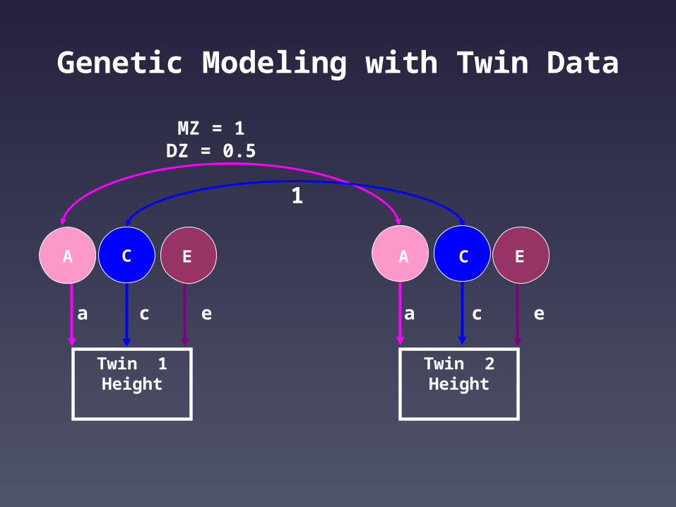
Genetic Modeling with Twin Data

a c a c

MZ = 1DZ = 0.5

1

A C

Twin 1Height

Twin 2Height

ee

E EC A

a11 a21

c11 c22

c21

e11 e21

e22

a11

a22a21

c11 c22

c21

e11e21

e22

MZ = 1DZ = 0.5

MZ = 1DZ = 0.5

1 1

C1 C2 C1 C2

Twin 1Height

Twin 1 Weight

Twin 2Height

Twin 2Weight

E1E2E1E2

a22

Bivariate Genetic Modeling

A1 A2 A1 A2

Building the Bivariate Genetic ModelSources of Information

• Cross-trait covariance within individuals– Within-Twin Covariance

• Cross-trait covariance between twins– Cross-Twin Covariance

• MZ:DZ ratio of cross-trait covariance between twins

Alternative Representations


X1 Y1

X1 VX1 CX1Y1

Y1 CY1X1 VY1

twin 1

twin 1


X1 Y1

X1 a112 CX1Y1

Y1 CY1X1 VY1

twin 1

twin 1


X1 Y1

X1 a112 CX1Y1

Y1 a21*a11 VY1

twin 1

twin 1


X1 Y1

X1 a112 a21*a11

Y1 a21*a11 VY1

twin 1

twin 1


X1 Y1

X1 a112 a21*a11

Y1 a21*a11 a222+a21

2

twin 1

twin 1


X1 Y1

X1 a112

+e 11

2 a21*a11+ e21*e11

Y1a21*a11+ e21*e11

a222+a21

2+e222+e2

12

twin 1

twin 1


X1 Y1

X2 CX2X1 CX2Y1

Y2 CY2X1 CY2Y1

twin 1

twin 2


X1 Y1

X2 1/0.5 * a112 CX2Y1

Y2 CY2X1 CY2Y1

twin 1

twin 2


X1 Y1

X2 1/0.5 * a112 CX2Y1

Y2 1/0.5 * a21*a11 CY2Y1

twin 2

twin 1


X1 Y1

X2 1/0.5 * a112 1/0.5 * a21*a11

Y2 1/0.5 * a21*a11 CY2Y1

twin 2

twin 1


X1 Y1

X2 1/0.5* a112 1/0.5 * a21*a11

Y2 1/0.5 * a21*a11

1/0.5*a222+1/0.5*a

212

twin 2

twin 1


X1 Y1 X2 Y2





twin 1

twin 1

twin 2

twin 2

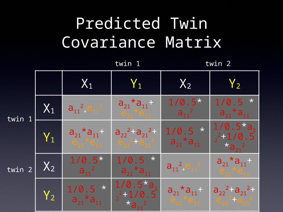
Predicted Twin Covariance Matrix

X1 Y1 X2 Y2

X1 a112

+e112 a21*a11+

e21*e11

1/0.5* a11

21/0.5 * a21*a11

Y1a21*a11+ e21*e11

a222+a21

2

+ e22

2+e212

1/0.5 * a21*a11

1/0.5*a222

+1/0.5*a21

2

X21/0.5*

a112

1/0.5 * a21*a11

a112

+e112 a21*a11+

e21*e11

Y21/0.5 * a21*a11

1/0.5*a222

+1/0.5*a21

2

a21*a11+ e21*e11

a222+a21

2

+ e22

2+e212

twin 1

twin 1

twin 2

twin 2

Predicted MZ Twin Covariance

X1 Y1 X2 Y2

X1 a112

+e112 a21*a11+

e21*e11a11

2 a21*a11

Y1a21*a11+ e21*e11

a222+a21

2

+ e22

2+e212

a21*a11 a222+a21

2

X2 a112 a21*a11 a11

2+e11

2 a21*a11+ e21*e11

Y2 a21*a11 a222+a21

2 a21*a11+ e21*e11

a222+a21

2

+ e22

2+e212

twin 1

twin 1

twin 2

twin 2

Predicted DZ Twin Covariance

X1 Y1 X2 Y2

X1 a112

+e112 a21*a11+

e21*e110.5*a11

2 0.5*a21*a11

Y1a21*a11+ e21*e11

a222+a21

2

+ e22

2+e212

0.5*a21*a11

0.5*a222+

0.5* a212

X2 0.5*a112 0.5*a21*a

11a11

2+e11

2 a21*a11+ e21*e11

Y20.5*a21*a

11

0.5*a222+

0.5* a212

a21*a11+ e21*e11

a222+a21

2

+ e22

2+e212

twin 1

twin 1

twin 2

twin 2

Predicted Covariance Matrix

X1 Y1 X2 Y2





twin 1

twin 1

twin 2

twin 2

Variances of X & Y same across twins and zygosity groups


X1 Y1 X2 Y2





twin 1

twin 1

twin 2

twin 2

Covariances of X & Y same across twins and zygosity groups


X1 Y1 X2 Y2





twin 1

twin 1

twin 2

twin 2

Cross-Twin Within-Trait Covariances differ by zygosity


X1 Y1 X2 Y2





twin 1

twin 1

twin 2

twin 2

Cross-Twin Cross-Trait Covariances differ by zygosity

OpenMx Specification

X1 Y1 X2 Y2

X1 VX1

CX1Y1

CX1X2

CX1Y2

Y1 CY1X1

VY1

CY1X2

CY1Y2

X2 CX2X1

CX2Y1

VX2

CX2Y2

Y2 CY2X1

CY2Y1

CY2X2

VY2

OpenMx script

Read in and Transform Variable(s)

transform variables to make variances with similar order of magnitudes

# Load Datadata(twinData)describe(twinData)twinData[,'ht1'] <- twinData[,'ht1']*10twinData[,'ht2'] <- twinData[,'ht2']*10twinData[,'wt1'] <- twinData[,'wt1']/10twinData[,'wt2'] <- twinData[,'wt2']/10

# Select Variables for AnalysisVars <- c('ht','wt')nv <- 2 # number of variablesntv <- nv*2 # number of total variablesselVars <- paste(Vars,c(rep(1,nv),rep(2,nv)),sep="") #c('ht1','wt1,'ht2','wt2')

# Select Data for AnalysismzData <- subset(twinData, zyg==1, selVars)dzData <- subset(twinData, zyg==3, selVars)

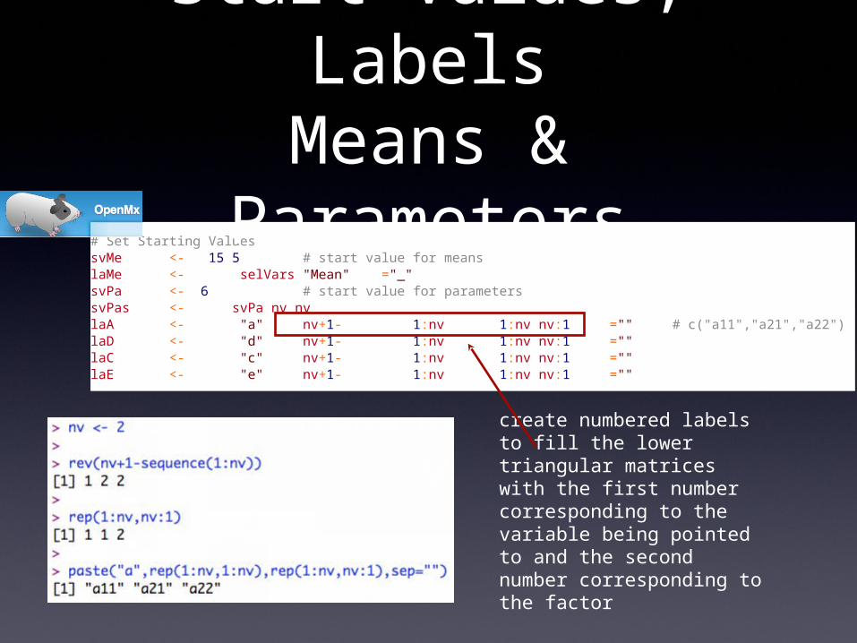
# Set Starting ValuessvMe <- c(15,5) # start value for meanslaMe <- paste(selVars,"Mean",sep="_")svPa <- .6 # start value for parameterssvPas <- diag(svPa,nv,nv)laA <- paste("a",rev(nv+1-sequence(1:nv)),rep(1:nv,nv:1),sep="") # c("a11","a21","a22")laD <- paste("d",rev(nv+1-sequence(1:nv)),rep(1:nv,nv:1),sep="")laC <- paste("c",rev(nv+1-sequence(1:nv)),rep(1:nv,nv:1),sep="")laE <- paste("e",rev(nv+1-sequence(1:nv)),rep(1:nv,nv:1),sep="")

Start Values, LabelsMeans &

Parameters

create numbered labels to fill the lower triangular matrices with the first number corresponding to the variable being pointed to and the second number corresponding to the factor

Within-Twin Covariance [A]

Path Tracing: Matrix Algebra: Lower 2x2

A1 A2

P1

P2

# Matrices declared to store a, c, and e Path CoefficientspathA <- mxMatrix( type="Lower", nrow=nv, ncol=nv, free=T, values=svPas, label=laA, name="a" ) pathD <- mxMatrix( type="Lower", nrow=nv, ncol=nv, free=T, values=svPas, label=laD, name="d" ) pathC <- mxMatrix( type="Lower", nrow=nv, ncol=nv, free=F, values=0, label=laC, name="c" )pathE <- mxMatrix( type="Lower", nrow=nv, ncol=nv, free=T, values=svPas, label=laE, name="e" ) # Matrices generated to hold A, C, and E computed Variance ComponentscovA <- mxAlgebra( expression=a %*% t(a), name="A" )covD <- mxAlgebra( expression=d %*% t(d), name="D" )covC <- mxAlgebra( expression=c %*% t(c), name="C" )covE <- mxAlgebra( expression=e %*% t(e), name="E" )

Path CoefficientsVariance

Components

regular multiplication of lower triangular matrix and its transpose

A1 A2

P1

P2

a %*% t(a)

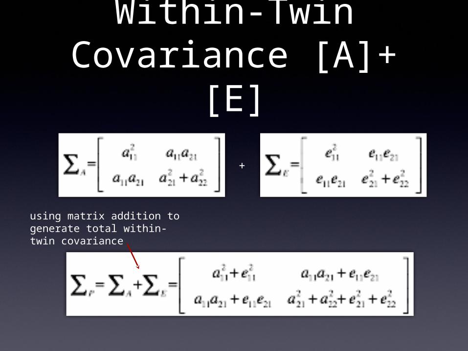
Within-Twin Covariance [A]+[E]

+

using matrix addition to generate total within-twin covariance

# Algebra to compute total variances and standard deviations (diagonal only)covP <- mxAlgebra( expression=A+D+C+E, name="V" )matI <- mxMatrix( type="Iden", nrow=nv, ncol=nv, name="I")invSD <- mxAlgebra( expression=solve(sqrt(I*V)), name="iSD")

# Algebras generated to hold Parameter Estimates and Derived Variance ComponentsrowVars <- rep('vars',nv)colVars <- rep(c('A','D','C','E','SA','SD','SC','SE'),each=nv)estVars <- mxAlgebra( cbind(A,D,C,E,A/V,D/V,C/V,E/V), name="Vars", dimnames=list(rowVars,colVars))

Total VariancesVariance

Components

each of covariance matrices is of size nv x nv

Cross-Twin Covariances [A] &

0.5[A]

+

using Kronecker product to multiple every element of matrix by scalar

# Algebra for expected Mean and Variance/Covariance Matrices in MZ & DZ twinsmeanG <- mxMatrix( type="Full", nrow=1, ncol=nv, free=T, values=svMe, labels=laMe, name="Mean" )meanT <- mxAlgebra( cbind(Mean,Mean), name="expMean" )covMZ <- mxAlgebra( rbind( cbind(V , A+D+C), cbind(A+D+C , V )), name="expCovMZ" )covDZ <- mxAlgebra( rbind( cbind(V , 0.5%x%A+0.25%x%D+C), cbind(0.5%x%A+0.25%x%D+C , V )), name="expCovDZ" )

Expected Means& Covariances

cbind creates two nv x ntv row matricesrbind turns them into to ntv x ntv matrix

# Data objects for Multiple GroupsdataMZ <- mxData( observed=mzData, type="raw" )dataDZ <- mxData( observed=dzData, type="raw" )

# Objective objects for Multiple GroupsobjMZ <- mxFIMLObjective( covariance="expCovMZ", means="expMean", dimnames=selVars )objDZ <- mxFIMLObjective( covariance="expCovDZ", means="expMean", dimnames=selVars )

# Combine Groupspars <- list( pathA, pathD, pathC, pathE, covA, covD, covC, covE, covP, matI, invSD, estVars, meanG, meanT )modelMZ <- mxModel( pars, covMZ, dataMZ, objMZ, name="MZ" )modelDZ <- mxModel( pars, covDZ, dataDZ, objDZ, name="DZ" )minus2ll <- mxAlgebra( expression=MZ.objective + DZ.objective, name="m2LL" )obj <- mxAlgebraObjective( "m2LL" )BivAceModel <- mxModel( "BivACE", pars, modelMZ, modelDZ, minus2ll, obj )

Data, Objectives & Model Objects

expected covariances and meansobserved data

# Run Bivariate ACE modelBivAceFit <- mxRun(BivAceModel)BivAceSum <- summary(BivAceFit)BivAceSum$paround(BivAceFit@output$estimate,4)round(BivAceFit$Vars@result,4)BivAceSum$Mi

# Generate Output with Functionssource("GenEpiHelperFunctions.R")parameterSpecifications(BivAceFit)expectedMeansCovariances(BivAceFit)tableFitStatistics(BivAceFit)

Parameter EstimatesVariance

Componentstwo ways to get parameter estimates

print pre-calculated unstandardized variance components and standardized variance components

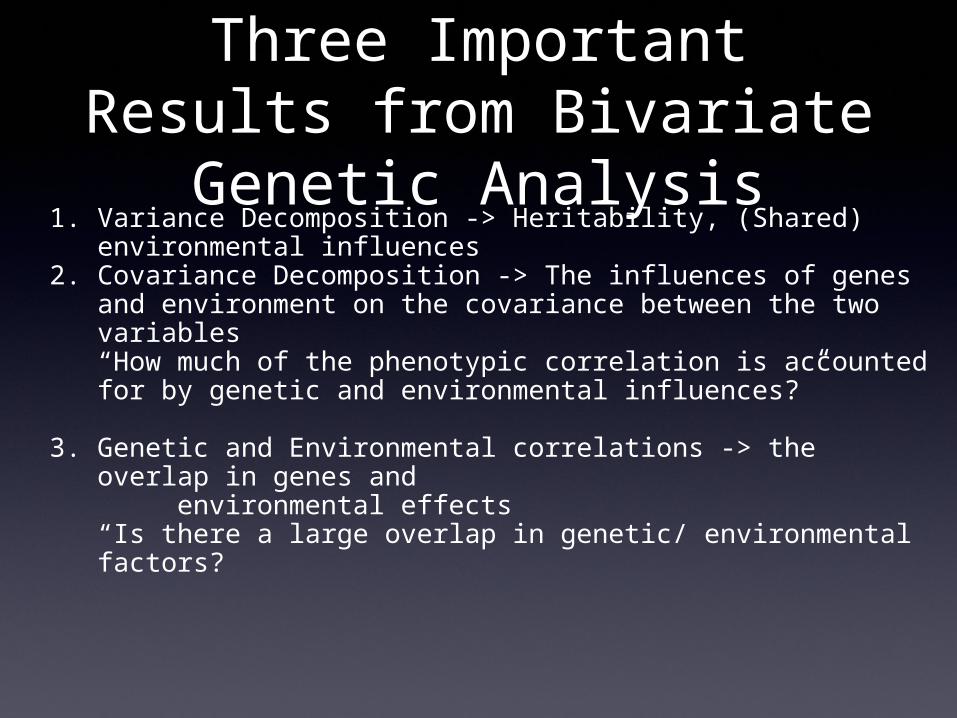
Three Important Results from Bivariate Genetic Analysis

1. Variance Decomposition -> Heritability, (Shared) environmental influences2. Covariance Decomposition -> The influences of genes and environment on

the covariance between the two variables“How much of the phenotypic correlation is accounted for by genetic and environmental influences?”

3. Genetic and Environmental correlations -> the overlap in genes and environmental effects

“Is there a large overlap in genetic/ environmental factors?

From Cholesky to Genetic Correlation

standardized solution = correlated factors solution

Genetic Covariance to Genetic Correlation

calculated by dividing genetic covariance by square root of product of genetic variances of two variables

# Calculate genetic and environmental correlationscorA <- mxAlgebra( expression=solve(sqrt(I*A))%&%A), name ="rA" )corD <- mxAlgebra( expression=solve(sqrt(I*D))%&%E), name ="rD" )corC <- mxAlgebra( expression=solve(sqrt(I*C))%&%C), name ="rC" )corE <- mxAlgebra( expression=solve(sqrt(I*E))%&%E), name ="rE" )

Genetic CorrelationAlgebra

72

Contribution to Phenotypic Correlation

if rg=1, then two sets of genes overlap completely

if however, a11 and a22 are near to zero, genes do not contribute much to phenotypic correlation

contribution to phenotypic correlation is function of both heritabilities and rg

Interpreting Results

• High genetic correlation = large overlap in genetic effects on the two phenotypes

• Does it mean that the phenotypic correlation between the traits is largely due to genetic effects?

• No: the substantive importance of a particular rG depends the value of the correlation and the value of the A

2 paths i.e. importance is also determined by the heritability of each phenotype

Interpretation of CorrelationsConsider two traits with a phenotypic correlation (rP) of 0.40 :

h2P1 = 0.7 and h2

P2 = 0.6 with rG = .3

• Correlation due to additive genetic effects = ?

• Proportion of phenotypic correlation attributable to additive genetic effects = ?

h2P1 = 0.2 and h2

P2 = 0.3 with rG = 0.8

• Correlation due to additive genetic effects = ?

• Proportion of phenotypic correlation attributable to additive genetic effects = ?

Correlation due to A:

Divide by rP to find proportion of phenotypic correlation.

Bivariate Cholesky Multivariate Cholesky

Fitting Bivariate Models October 21, 2014 Elizabeth Prom-Wormley & Hermine Maes [email protected]...

Documents

Transcript of Fitting Bivariate Models October 21, 2014 Elizabeth Prom-Wormley & Hermine Maes [email protected]...