Fitting B-spline Curves to Point Clouds by Curvature-Based ... · by Curvature-Based Squared...

Fitting B-spline Curves to Point Clouds

by Curvature-Based Squared Distance Minimization

Wenping Wang

University of Hong Kong

Helmut Pottmann

Vienna University of Technology

and

Yang Liu

University of Hong Kong

Computing a curve to approximate data points is a problem encountered frequently in many ap-plications in computer graphics, computer vision, CAD/CAM, and image processing. We present

a novel and efficient method, called squared distance minimization (SDM), for computing a planarB-spline curve, closed or open, to approximate a target shape defined by a point cloud, i.e., a set

of unorganized, possibly noisy data points. We show that SDM outperforms significantly otheroptimization methods used currently in common practice of curve fitting. In SDM a B-spline curvestarts from some properly specified initial shape and converges towards the target shape throughiterative quadratic minimization of the fitting error. Our contribution is the introduction of anew fitting error term, called the squared distance (SD) error term, defined by a curvature-basedquadratic approximant of squared distances from data points to a fitting curve. The SD error term

measures faithfully the geometric distance between a fitting curve and a target shape, thus leadingto faster and more stable convergence than the point distance (PD) error term, which is commonly

used in computer graphics and CAGD, and the tangent distance (TD) error term, which is oftenadopted in the computer vision community. To provide a theoretical explanation of the superiorperformance of SDM, we formulate the B-spline curve fitting problem as a nonlinear least squares

problem and conclude that SDM is a quasi-Newton method, which employs a curvature-basedpositive definite approximant to the true Hessian of the objective function. Furthermore, we show

that the method based on the TD error term is a Gauss-Newton iteration, which is unstable fortarget shapes with high curvature variations, whereas optimization based on the PD error term isthe alternating method that is known to have linear convergence.

Categories and Subject Descriptors: I.3.5 [Computer Graphics]: Computational Geometry and Object Modeling—Curve,

surface, solid, and object representations; J.6 [Computer-Aided Engineering]: Computer-aided design (CAD); G.1.6 [Nu-

merical Analysis]: Optimization—Least squares methods

General Terms: Shape reconstruction, scatter data approximation

Additional Key Words and Phrases: B-spline curve, curve fitting, point cloud, least squaresproblem, optimization, squared distance, Gauss-Newton method, quasi-Newton method

Authors’ address: Wenping Wang, Department of Computer Science, The University of Hong Kong, Pokfulam Road, HongKong, China; email [email protected]; Helmut Pottmann, Institute of Discrete Mathematics and Geometry, Vienna University

of Technology, Wien, Austria; email [email protected]; Yang Liu, Department of Computer Science, TheUniversity of Hong Kong, Pokfulam Road, Hong Kong, China; email: [email protected]. The work of the first author was

partially supported by a CRCG grant from The University of Hong Kong. The second author acknowledges support by theAustrian Science Fund under grant P16002-N05.Permission to make digital/hard copy of all or part of this material without fee for personal or classroom use provided that

the copies are not made or distributed for profit or commercial advantage, the ACM copyright/server notice, the title of thepublication, and its date appear, and notice is given that copying is by permission of the ACM, Inc. To copy otherwise, to

republish, to post on servers, or to redistribute to lists requires prior specific permission and/or a fee.c© 20YY ACM 0730-0301/20YY/0100-0001 $5.00

ACM Transactions on Graphics, Vol. V, No. N, Month 20YY, Pages 1–0??.

2 · Wenping Wang et al.

1. INTRODUCTION

We consider the following problem: Given a set of unorganized data points Xk, k = 1, 2, . . . , n, in the plane,compute a planar B-spline curve to approximate the points Xk. The data points Xk are assumed to representthe shape of some unknown planar curve, which can be open or closed, but not self-intersecting; this curve iscalled a target curve or target shape. We suppose that unorganized data points, often referred to as a pointcloud or scattered data points in literature, may have non-uniform distribution with considerable noise; thisassumption makes it difficult or impossible to order data points along the target curve. Hence, we assumethat such an ordering is not available.

The above problem can be formulated as a nonlinear optimization problem as follows. Consider a B-splinecurve P (t) =

∑mi=1 PiBi(t) with control points Pi. We assume throughout that the order and the knots of

the B-spline curve are fixed, so they are not subject to optimization. This simplifying assumption allowsus to give a clear explanation of the general idea of our new optimization scheme. The very same idea ofoptimization presented here can also be extended to the more general setting of fitting a NURBS curve withfree weights and knots to be optimized, by variable linearization and inequality constraints.

Given data points Xk, k = 1, 2, . . . , n, we want to find the control points Pi, i = 1, 2, . . . ,m, such that theobjective function

f =1

2

n∑

k=1

d2(P (t),Xk) + λfs (1)

is minimized, where d(P (t),Xk) = mint ||P (t) − Xk|| is the distance of the data point Xk to the curveP (t), fs is a regularization term to ensure a smooth solution curve and λ is a positive constant to modulatethe weight of fs. Here the distance d(P (t),Xk) is measured orthogonal to the curve P (t) from Xk. Theexceptional case where the shortest distance from Xk to an open curve P (t) occurs at an endpoint of P (t)will be discussed separately in Section 5.

We present a novel method that approximates unorganized data points with a B-spline curve that startswith some properly specified initial curve and converges through iterative optimization towards the targetshape of data points. One of our contributions is the introduction of a novel error term defined by a curvature-based quadratic approximant of squared distances from data points to the fitting curve. For brevity, this newerror term is called the squared distance error term or SD error term, and the resulting iterative minimizationscheme will be referred to as squared distance minimization or SDM. Because the SD error term measuresfaithfully the geometric distance between data points and the fitting curve, SDM converges fast and stably,in comparison with other commonly used error terms, as will be discussed shortly.

The remainder of the paper is organized as follows. We first review related previous work. Then weintroduce the SD error term, outline our SDM method, and use some test examples to show the superiorperformance of SDM in comparison with two other commonly used methods — point distance minimization(PDM) and tangent distance minimization (TDM). We will also discuss the B-spline curve fitting problemfrom the viewpoint of optimization to provide insights into the superior performance of SDM. We will showthat SDM is, in fact, a quasi-Newton method which employs a carefully chosen positive definite approximantto the true Hessian of the objective function. We will also show that TDM is a variant of the Gauss-Newtonmethod. Furthermore, PDM is, in fact, the alternating method for solving a separable problem and is knownto have only linear convergence [Ruhe and Wedin 1980; Bjorck 1996; Speer et al. 1998]. This systematic studyof the relationship between these geometrically motivated curve fitting methods and standard optimizationtechniques is another contribution of our work.

ACM Transactions on Graphics, Vol. V, No. N, Month 20YY.

Fitting B-spline Curves by SDM · 3

2. RELATED WORK

2.1 Spline curve fitting techniques

Fitting a curve to a set of data points is a fundamental problem in graphics (e.g., [Pavlidis 1983; Plass andStone 1983; Pratt 1985; Walton and Xu 1991; Goshtasby 2000]) and many other application areas. Insteadof attempting a comprehensive review, we will only discuss some main results in the literature to provide abackground for our work.

Let Xk ∈ R2, k = 1, 2, . . . , n, be unorganized data points representing a target shape, which is to beapproximated by a closed or open planar B-spline curve P (t) =

∑mi=1 Bi(t)Pi, where the Bi(t) are the B-

spline basis functions of a fixed order and knots, and the Pi are the control points. Since f in Eqn. (1) is anonlinear objective function, iterative minimization comes as a natural approach. Suppose that we have aspecific B-spline curve Pc(t) =

∑mi=1 Bi(t)Pc,i with control points Pc = (Pc,1, Pc,2, . . . , Pc,m), which can be

an initial fitting curve or the current fitting generated from the last iteration. Let D = (D1,D2, ..,Dm) bethe variable updates to Pc to give the new control points P+ = Pc + D. Let P+(t) =

∑mi=1 Bi(t)(Pc,i + Di)

denote the B-spline curve with updated control points P+.Many existing B-spline curve fitting methods invoke a data parameterization procedure to assign a pa-

rameter value tk to each data point Xk. In some methods dealing with ordered data points, the chordlength method or the centripetal method [Lee 1989; Hoschek and Lasser 1993; Farin 1997] are used for dataparameterization. Then, with the fixed tk, the function

f =1

2

∑

k

||P+(tk) − Xk||2 + λfs, (2)

which is a local quadratic model of f in (1), is minimized by solving a linear system of equations to yieldupdated control points P+, and hence the updated fitting curve P+(t).

A commonly used data parameterization method is to choose tk such that Pc(tk) is the closest point fromthe current fitting curve to the data point Xk; (Pc(tk) is also called the foot point of Xk on the curve Pc(t)).Then an iterative method can be developed by interleaving this step of foot point computation with theminimization of the local quadratic model f in (2) to compute the updated control points P+. Note that theerror term ||P+(tk)−Xk||

2 in (2) measures the squared distance between the data point Xk and a particularpoint P+(tk) on the fitting curve to be determined; therefore, we will call this error term the point distanceerror term or the PD error term, and denote it by

ePD,k = ||P+(tk) − Xk||2. (3)

(The PD error term is illustrated in Figure 1.) This minimization scheme will be called the point distanceminimization or PDM for short. Note that, since the ordering of data points is not required for dataparameterization via foot point projection, PDM is applicable to fitting a curve to a point cloud.

Hoschek [Hoschek 1988] proposes an iterative scheme, called intrinsic parameterization, which also usesthe PD error term but performs parameter correction using a formula that is a first-order approximationto exact foot point computation. Bercovier and Jacob [Bercovier and Jacob 1994] prove that the intrinsicparameterization method is equivalent to Uzawa’s method for solving a constrained minimization problem,but they do not establish the convergence rate of the intrinsic parameterization method or that of PDM.Higher order approximation or accurate computation of foot points for data parameterization are discussedin [Hoschek and Lasser 1993; Saux and Daniel 2003; Hu and Wallner 2005].

PDM, or its simple variants, are the most commonly applied method for curve fitting in computer graphicsand CAD [Plass and Stone 1983; Hoschek 1988; Goshtasby 2000; Saux and Daniel 2003]. The same idea ofPDM is also widely used for surface fitting [Hoppe et al. 1994; Forsey and Bartels 1995; Hoppe 1996; Ma andKruth 1995; Haber et al. 2001; Wang and Phillips 2002; Djebali et al. 2002; Greiner et al. 2002; Weiss et al.



2002; Maekawa and Ko 2002; Taubin 2002], with B-spline surfaces as well as other types of surfaces. Thepopularity of PDM might be explained by its simplicity — the error term ePD,k in (3) is derived by simplysubstituting tk in the squared distance d2(P (t),Xk) in the original objective function f in (1). However,considering that P (tk) is a variable point depending on the variable control points, ePD,k is a rather poorapproximation to d2(P (t),Xk), thus causing slow convergence. As a matter of fact, the present paper is justabout how to use a better approximation of d2(P (t),Xk) to devise a more efficient optimization scheme.

Another error term, often used in the computer vision community (e.g., [Blake and Isard 1998]), is definedby

eTD,k = [(P+(tk) − Xk)T Nk]2, (4)

where Nk is a unit normal vector of the current fitting curve Pc(t) at the point Pc(tk). We will call eTD,k

the tangent distance error term or the TD error term, since eTD,k gives the squared distance from Xk to thetangent of Pc(t) at the foot point Pc(tk) when P+(t) is Pc(t). The TD error term is illustrated in Figure 2.

The TD error term eTD,k = [(P+(tk) − Xk)T Nk]2 can also be combined with data parametrization viafoot point projection to yield a B-spline curve fitting method, as used in [Blake and Isard 1998] for boundaryextraction in motion tracking. We will call this method tangent distance minimization or TDM. TDMminimizes in each iteration the function

fTD =1

2

∑

k

eTD,k + λfs. (5)

Treating the control points P+ as variables to be optimized, the TD error term measures the squareddistance from the point Xk to a moving straight line Lk that has the fixed normal vector Nk and passesthrough the moving point P+(tk). See Figure 3. The TD error eTD,k = [(P+(tk)−Xk) ·Nk]2 becomes zero ifthe point Xk is contained in the line Lk. On the other hand, the line Lk is a relatively poor approximationto the curve P+(t) in a neighborhood of a high-curvature point P+(tk) or if Xk is far from P+(tk). Hence, inthese cases, the point Xk may still be poorly approximated by the curve P+(t) even if Xk is nearly on Lk,i.e., when the TD error [(P+(tk) − Xk) · Nk]2 is nearly zero (see Figure 3).

PD error

Xk

d

P+(tk)

Fig. 1. Iso-values curves of the point distance (PD)

error term.

TD error

Xk

d

P+(tk)

Fig. 2. Iso-values curves of the tangent distance

(TD) error term.

This disparity between approximation quality and error measurement is the cause of the instability ofTDM near a high-curvature part of the target shape, as will be illustrated later with test examples. Thisunstable behavior of TDM is, in fact, the consequence of using an inappropriately large step size to solve anonlinear optimization problem; indeed, we will show that TDM uses Gauss-Newton iteration for solving a



nonlinear least-squares problem and its excessively large step size is due to omission of important curvaturerelated parts in the true Hessian.

Now let us consider the geometric interpretations of the PD error term and the TD error term. SincePc(tk) is fixed foot point on the current fitting curve Pc(t) of Xk, if P+(t) is the same as Pc(t) then bothePD,k and eTD,k give the same value of d2(Pc(tk),Xk). However, for optimization purpose, we need toregard d2(P+(tk),Xk) as a function of variable control points P+, and in this sense ePD,k and eTD,k givevery different approximations to d2(P+(tk),Xk).

If treating Xk as a free point, for any constant c > 0, the iso-value curve ePD,k ≡ ||P+(tk) − Xk||2 = c of

the PD error term is a circle (see Figure 1), and the iso-value curve eTD,k ≡ [(P+(tk) − Xk) · Nk]2 = c ofthe TD error term is a pair of parallel lines, which can be regarded as a degenerate ellipse (see Figure 2).Since PDM has relatively slow convergence and TDM tends to have fast but unstable convergence, one mayspeculate whether or not a new error term with ellipse-shaped iso-value curves can be devised to yield amore balanced performance between efficiency and stability. We will see that such an error term is naturallyprovided by a curvature-based quadratic approximation to the squared distance function.

2.2 Second order approximation to squared distance function

Given a curve C in E2, one may define the squared distance function that assigns to each point X inE2 the squared distance from X to C. The second order approximation to this distance function is givenin [Ambrosio and Montegazza 1998]. This approximation is then studied in detail and applied to solving anumber of shape fitting problems in [Pottmann et al. 2002; Pottmann and Hofer 2003]. Below we reviewthis work briefly.

Let O be the closest point on a twice differentiable curve C to a fixed point X0 (see Figure 4). Considerthe local Frenet frame of C with its origin at O and its two coordinate axes being the tangent vector and thenormal vector of the curve C at O. Let ρ > 0 be the curvature radius of C at O. We use an orientation ofthe curve normal such that K = (0, ρ)T is the curvature center of C at O. Let d be the signed distance fromX0 to O, i.e., |d| = ||X0 − O|| with d < 0 if X0 and K are on opposite sides of the curve C, and d > 0 if X0

and K are on the same side of C. We note that there is always d < ρ when d > 0, for otherwise O cannotbe the closest point on the curve C to X0.

P+(tk)

Xk

d

Pc(tk)

Xk

d

Lk Lk

Fig. 3. In a neighborhood of a high curvature point, the

true approximation error can be rather big even when the

TD error d is small.

(0,ρ)

x

y

X0

O

d

Fig. 4. A second order approximant of the squared distancefunction to the curve C at X0.

Consider a point X = (x, y)T in a neighborhood of X0. The second order approximant of the squared



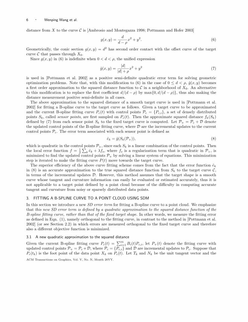
distance from X to the curve C is [Ambrosio and Montegazza 1998; Pottmann and Hofer 2003]

g(x, y) =d

d − ρx2 + y2. (6)

Geometrically, the conic section g(x, y) = d2 has second order contact with the offset curve of the targetcurve C that passes through X0.

Since g(x, y) in (6) is indefinite when 0 < d < ρ, the unified expression

g(x, y) =|d|

|d| + ρx2 + y2 (7)

is used in [Pottmann et al. 2002] as a positive semi-definite quadratic error term for solving geometricoptimization problems. Note that, with this modification to (6) in the case of 0 ≤ d < ρ, g(x, y) becomesa first order approximation to the squared distance function to C in a neighborhood of X0. An alternativeto this modification is to replace the first coefficient d/(d − ρ) by max{0, d/(d − ρ)}, thus also making thedistance measurement positive semi-definite in all cases.

The above approximation to the squared distance of a smooth target curve is used in [Pottmann et al.2002] for fitting a B-spline curve to the target curve as follows. Given a target curve to be approximatedand the current B-spline fitting curve Pc(t) with control points Pc = {Pc,i}, a set of densely distributedpoints Sk, called sensor points, are first sampled on Pc(t). Then the approximate squared distance fk(Sk)defined by (7) from each sensor point Sk to the fixed target curve is computed. Let P+ = Pc + D denotethe updated control points of the B-spline fitting curve, where D are the incremental updates to the currentcontrol points Pc. The error term associated with each sensor point is defined as

ek = g(Sk(P+)), (8)

which is quadratic in the control points P+, since each Sk is a linear combination of the control points. Thenthe local error function f = 1

2

∑k ek + λfs, where fs is a regularization term that is quadratic in P+, is

minimized to find the updated control points P+ by solving a linear system of equations. This minimizationstep is iterated to make the fitting curve P (t) move towards the target curve.

The superior efficiency of the above curve fitting scheme comes from the fact that the error function ek

in (8) is an accurate approximation to the true squared distance function from Sk to the target curve C,in terms of the incremental updates D. However, this method assumes that the target shape is a smoothcurve whose tangent and curvature information can easily be evaluated or estimated accurately, thus it isnot applicable to a target point defined by a point cloud because of the difficulty in computing accuratetangent and curvature from noisy or sparsely distributed data points.

3. FITTING A B-SPLINE CURVE TO A POINT CLOUD USING SDM

In this section we introduce a new SD error term for fitting a B-spline curve to a point cloud. We emphasizethat this new SD error term is defined by a quadratic approximation to the squared distance function of theB-spline fitting curve, rather than that of the fixed target shape. In other words, we measure the fitting erroras defined in Eqn. (1), namely orthogonal to the fitting curve, in contrast to the method in [Pottmann et al.2002] (or see Section 2.2) in which errors are measured orthogonal to the fixed target curve and thereforealso a different objective function is minimized.

3.1 A new quadratic approximation to the squared distance

Given the current B-spline fitting curve Pc(t) =∑m

i=1 Bi(t)Pc,i, let P+(t) denote the fitting curve withupdated control points P+ = Pc +D, where Pc = {Pc,i} and D are incremental updates to Pc. Suppose thatPc(tk) is the foot point of the data point Xk on Pc(t). Let Tk and Nk be the unit tangent vector and the



unit normal vector of the current fitting curve Pc(t) at the foot point Pc(tk), ρ > 0 is the curvature radius ofPc(t) at Pc(tk) and |d| = ‖Pc(tk) − Xk‖, with the same convention on the sign of d as made in Section 2.2.When the control points P+ change, with the same parameter tk, the foot point Pc(tk) becomes a variablepoint P+(tk), and the unit tangent vector Tk, the unit normal vector Nk and curvature radius ρ of the curveP+(t) at the point P+(tk) all vary with P+.

To obtain a quadratic approximation to the squared distance from Xk to the curve P+(t), we assume thatTk, Nk and ρ are fixed to be Tk, Nk and ρ, i.e., they do not vary with P+. This assumption implies that,locally at the point Pc(tk), we will only consider a differential translation of the curve Pc(t) into the curveP+(t). Since this translation is relative to the data point Xk, we may view, in a relative sense, that P+(t)is a fixed curve and Xk undergoes a translation. Therefore, we may use the formula (6) to approximate thesquared distance from Xk to the curve P+(t), expressed in the global coordinate system, as

hk(D) =d

d − ρ[(P+(tk) − Xk)T Tk]2 + [(P+(tk) − Xk)T Nk]2. (9)

Note that hk(D) may take a negative value when 0 < d < ρ. In order to obtain a positive semi-definiteerror metric, based on hk(D), we define the new error term as

eSD,k(D) =

{d

d−ρ [(P+(tk) − Xk)T Tk]2 + [(P+(tk) − Xk)T Nk]2, if d < 0,

[(P+(tk) − Xk)T Nk]2, if 0 ≤ d < ρ,

(10)

Clearly, eSD,k(D) is a positive semi-definite quadratic function of D in all cases. Since eSD,k(D) is derivedfrom a direct attempt to accurately approximate the squared distance function, we will call eSD,k(D) thesquared distance error term or SD error term for short. We stress that, due to the simplifications we havemade, eSD,k(D) is, in general, no longer a second order approximation to the squared distance function, butrather a first order approximation that is more accurate than the PD error term or the TD error term.

When d < 0, the level-set curve of eSD,k(D) = c is an ellipse centered at the point P+(tk), if the Xk

is treated as a variable point. When the control points P+ change, the ellipse is translated by keeping itscenter at P+(tk) but with its shape, size and orientation remaining unchanged (see Figure 5). The SD errorterm eSD,k becomes the TD error term eTD,k when 0 ≤ d < ρ, i.e., when (i) the data point Xk is sufficientlynear Pc(tk) relative to the magnitude of ρ; and (ii) Xk is on the convex side of the curve Pc(t), i.e., Xk andthe curvature center K are on the same side of the curve Pc(t). The use of the TD error term here will notcause instability, since in this case the tangent line is a relatively good approximation to the curve Pc(t) ina neighborhood of Pc(tk).

Iterative minimization of the squared distance using the SD error term (10), interleaved with foot pointcomputation for data parameterization, will be called squared distance minimization or SDM. Although thetangent and normal vectors Tk and Nk, as well as ρ, are kept fixed during an iteration, they are updated atthe beginning of each iteration to reflect the continual change of the shape of the fitting curve.

The above derivation of the SD error term is based on a geometric argument. Using a second order Taylorexpansion, we will reveal the relationship between this SD error term and the Newton iteration later inSection 6.3, thus providing another derivation of the SD error term.

3.2 Main steps of SDM

The main steps of the SDM method are as follows.

(1) Specify a proper initial shape of a B-spline fitting curve.

(2) Compute SD error terms for all data points to obtain a local quadratic approximation fSD of the objective



Xk

(a) (b)

Xk

PD(tk)

P(tk)

Fig. 5. The SD error term eSD,k(D) defined by (10) is shown via its iso-value curves in the case of d < 0. (a) Before updating

the control points P. (b) The translation of eSD,k(D) after updating P.

function f , defined by

fSD =1

2

∑

k

eSD,k + λfs.

(3) Solve a linear system of equations to minimize fSD to obtain an updated B-spline fitting curve.

(4) Repeat steps 2 and 3 until convergence, i.e., until a pre-specified error threshold is satisfied or theincremental change of the control points falls below a preset threshold.

4. EXPERIMENTS AND COMPARISON

In this section we use some test examples to compare SDM with PDM and TDM for fitting a closed B-splinecurve to unorganized data points in the plane. The quadratic function to be optimized in each iteration hasthe form

f =1

2

n∑

k=1

ek + αF1 + βF2, (11)

where ek is a particular error term (PD, TD or SD) for the data point Xk, F1 and F2 are energy termsdefined as

F1 =

∫‖P ′(t)‖2dt, F2 =

∫‖P ′′(t)‖2dt, (12)

and α, β ≥ 0 are constants. In our implementation F1 and F2 are integrated explicitly without numericalapproximation.

For a fixed B-spline fitting curve P (t), the Euclidean distance from data point Xk to P (t) is denoted bydk = ‖P (tk) − Xk‖, where P (tk) is the foot point of Xk on P (t). Then, for evaluating the approximationerror, we define the average error, which is the root mean square error, as

Error Ave =

[1

n

n∑

k=1

d2k

]1/2

,

and the maximum error as

Error Max =n

maxk=1

{dk}.

We present below the results of applying the three methods — PDM, TDM and SDM — to fitting a cubicB-spline curve with uniform knots to several sets of unorganized data points. The same values of energycoefficients α = 0 and β = 0.001 are used for all the examples in this section, unless specified otherwise.



(a) Data points on a circle

and an initial B-spline curve.

(b) The fitting curve gener-

ated by PDM in 10 iterations.

(c) The fitting curve gener-

ated by TDM in 10 iterations.

(d) The fitting curve gener-

ated by SDM in 10 iterations.

0.5 1 1.5 2 2.5

-1

log10

(Error_Ave)

log10

(# of iterations)

PDM

TDM

SDM

-1.5

-2

-2.5

-0.5

(e) The average error versus the number of iterations of

the three methods.

0.5 1 1.5 2 2.5

-2.5

-2

-1.5

-1

-0.5

PDM

TDM

SDM

log10

(Error_Max)

log10

(# of iterations)

(f) The maximum error versus the number of iterations

of the three methods.

Fig. 6. (Example 1) Comparison of the three methods on a set of 32 sparse data points on a circle. In this figure log scale (base10) is used for the iteration axis in Figures (e) and (f) in order to distinguish the error curves of TDM and SDM.

Example 1. Non-uniform data points on a circle. (See Figure 6.) TDM and SDM converge with roughlythe same speed, and both converge much faster than PDM does, as shown in Figures 6(e) and (f). PDMtakes about 100 iterations to reach the same small error values produced by SDM in fewer than 10 iterations.

Example 2. (See Figure 7.) For this set of data points, SDM again converges much faster than PDMdoes, while TDM is trapped in a local minimum, producing a curve with self-intersection. To visualizethe evolution of an iterative optimization process (PDM or SDM), we place the fitting curves generated insuccessive iterations at successive heights to form an evolution surface (see Figure 8). Data points or a subsetof them are displayed at the top of an evolution surface. A striped texture is used to depict the trajectoriesof points of fixed parameter values on the fitting curve. The trajectories of evolving control points are shownby white curves in space. Log scale (base 10) is used for the height axis in these figures to accommodate forthe large number of iterations needed by PDM. For size reference, a base square of size 2.2 × 2.2 is shownalong with these evolution surfaces.

The evolution surfaces generated by PDM and SDM (Figure 8), viewed from two different directions, showthat PDM experiences a slow convergence process, while SDM converges quickly with conspicuous tangentflow of the control points in the first 10 iterations.

Example 3. (See Figure 9.) This set of data points is extremely noisy. After 50 iterations, SDM hasalready produced an acceptable result, while PDM converges slowly and TDM becomes unstable. Herestrong tangential flow of control points is observed in SDM to move some control points at the bottom ofthe initial curve to the top in (d).



(a) Unorganized data points

on a “C” shape and an initial

B-spline curve.







100 200 300 400 500

-1.8

-1.6

-1.4

-1.2

-1

-0.8

log10

(Error_Ave)

# of iterations

PDM

TDM

SDM

(e) The average error versus the number of iterations of

the three methods.

100 200 300 400 500

-1.6

-1.4

-1.2

-0.8

-0.6

-0.4

log10

(Error_Max)

# of iterations

PDM

TDM

SDM

(f) The maximum error versus the number of iterations

of the three methods.

Fig. 7. (Example 2) Comparison of the three methods on a set of 102 data points. SDM converges faster than PDM does.TDM is trapped in a local minimum with self-intersection in the fitting curve.

Example 4. (See Figure 10.) The difficulty with this test lies in the corner points of the target shape andthe highly non-uniform distribution of the control points of the initial B-spline curve. After 20 iterations,PDM gets trapped in an unacceptable local minimum and TDM becomes divergent, while SDM convergessuccessfully. Again SDM exhibits strong tangential flow responsible for re-distributing control points initiallyclustered at one side on the initial curve over the target shape to well approximate the four corner points.

The four examples above are from numerous examples with which we have experimented. The followingobservations can be made from our experiments.

1) PDM exhibits the slowest convergence among the three methods, and is often trapped at a poor localminimum. Our experiments confirm the theoretical conclusion that PDM has, in general, only linearconvergence. This is further explained in Section 6.

2) TDM demonstrates fast convergence when the target shape is not so noisy (i.e., representing a small-residue problem) and the initial fitting curve is relatively near the target shape (i.e., |d| ≤ ρ), but oftenbecomes unstable or even develops self-intersection in a high curvature region of the target shape or if theinitial fitting curve is relatively far from the target shape. Increasing the value of the energy coefficientβ in (11) usually improve the stability of TDM, as well as the fairness of the fitting curve, but often atthe expense of a larger fitting error.

3) SDM exhibits much faster convergence than PDM does. The convergence of SDM is about as fast as



(a) PDM (b) SDM

(c) PDM (d) SDM

Fig. 8. The evolution surfaces of PDM and SDM for the data in Example 2 (Figure 7) — viewed from two different angles. (a)

The evolution surface of PDM; (b) The evolution surface of SDM with the same view angle as in (a); (c) The evolution surfaceof PDM from another view angle; (d) The evolution surface of SDM with the same view angle as in (c).

that of TDM; moreover, SDM is more stable than TDM, since TDM often does not converge for targetshapes with shape features. This is mainly due to the fact that TDM is a Gauss-Newton method withoutstep size control. We will discuss this in more detail in Section 6.

4) The iso-value curves of the SD error term are ellipses aligned with the tangent at a point of the fittingcurve. Therefore, at a low-curvature region of a B-spline fitting curve, the control points of the fittingcurve, as well as points on the fitting curve, can flow in the tangential direction to attain a betterdistribution without causing much penalty from the SD error term. Meanwhile, as desired, such a flow



(a) A closed target shape and

an initial B-spline curve.







Fig. 9. (Example 3) Comparison of the three methods for fitting an extremely noisy data set of 1, 630 points. After 50 iterations,SDM generates a satisfactory fitting curve (d), but TDM becomes unstable (c), and PDM is still improving at a slow rate (b);PDM needs about 400 iterations to produce a fitting curve similar to the one by SDM shown in (d).

(a) A square-shaped target

shape and an initial B-spline

curve.







Fig. 10. (Example 4) Comparison of the three methods for approximating a square-shaped target shape consisting of 33 datapoints. PDM is trapped in a poor local minimum (b), TDM eventually becomes divergent (c), and SDM converges successfully

in 20 iterations.

is dampened at a high-curvature region due to the role played by the curvature radius ρ and distance din the SD error term. In contrast, tangential flow of control points is inhibited by the PD error term,causing stagnant improvement. Meanwhile, this tangential flow is checked nowhere by the TD errorterm, since the TD error term ignores curvature variation on the fitting curve, thus leading to unstableconvergence in the presence of corner points in the target shape.

The ease of implementation and per-iteration computation time of SDM are nearly the same as thoseof PDM and TDM, since the three methods share the same framework but use different quadratic errorterms. The per-iteration computation time of SDM is mainly determined by the number of data points. Thedominant part of computation time is the computation of the foot points of all data points in each iteration.For example, for the set of 1,630 data points used in Example 3, computation of each iteration takes about0.15 seconds on a PC with Pentium IV 2.4GHz CPU and 256 MB RAM, with over 95% of this time spenton foot point computation.



5. IMPLEMENTATION ISSUES

In this section we discuss the following implementation issues for facilitating the convergence or improvingthe computational efficiency of SDM: 1) initialization and adjustment of control points; 2) fast setup of errorterms; and 3) adapting SDM to fit an open B-spline curve to data points.

5.1 Initialization and adjustment of control points

All the three methods we have discussed so far, PDM, TDM and SDM, are local minimization schemes; thatis to say, their convergence depends on the initial value, i.e., the initial fitting curve. We would like to pointout several possibilities of specification of the initial fitting curve, though this is not a focus of the presentpaper. The first obvious option is to let the user specify an initial B-spline fitting curve that is sufficientlyclose to the target shape and has an appropriate number of control points.

For a target shape defined by a set of dense points, an alternative is to compute a quadtree partition ofthe data points and then extract a sequence of points approximating the target shape from non-empty cells,i.e., those cells containing at least one data point. These extracted points can then be used as the controlpoints of an initial B-spline fitting curve. Our experience shows that this method tends to produce too manycontrol points at the beginning, so control point deletion is normally required during the fitting process inorder to obtain a fitting curve with a minimal number of control points while still meeting a prescribed errorthreshold.

Another approach under our current investigation is based the active contour model. In this method, asimple initial fitting curve is specified either automatically or by the user. Then some external energy/force isused in combination with SDM to drive the fitting curve to converge to a complex target shape in a mannerthat ensures global convergence. The key issues here are (i) proper design of the external force so thatfeatures and concavities of the target shape can be captured; and (ii) progressive insertion of control pointsat appropriate locations and stages so as to provide increasing shape flexibility to cope with the complexityof the target shape. The details of this procedure are beyond the scope of the present paper and we wish toreport on them in a separate paper. We refer to [Yang et al. 2004] for discussions on control point insertionand deletion in the context of a local B-spline curve fitting procedure.

5.2 Fast setup of error terms

Efficient computation of foot points on the fitting curve of data points is important, especially when theyare a large number of data points, since an error term needs to be computed for each data point in everyiteration. We use the following speedup method consisting of two phases: preprocessing and query. Inpreprocessing we first compute a uniform spatial partition of the data points with a proper cell size andrecord those nonempty cells. Next we sample a sufficient number of points on the fitting curve and computethe normal lines of the fitting curve at these sample points. Then we record the intersections between thesenormal lines and all the non-empty cells.

In the query phase, for each data point Xk, we find its containing cell and the two normal lines suchthat Xk is between the two lines and they are closest to Xk (see Figure 11). Let the two normal lines beassociated with parameter values t1 and t2 of the fitting curve. Let d1 and d2 denote the distances from Xk

to the two lines. Then, supposing that the current fitting curve is sufficiently close to the target shape, agood estimate P (tk) of the foot-point of Xk is given by linear interpolation tk = (d2t1 +d1t2)/(d1 +d2). Thepoint P (tk) is then used as an initial point in a Newton-like iterative procedure to find the foot point P (tk)of Xk.

Figure 13 shows an example of using SDM and PDM to fit a B-spline curve to the contour of a Chinesecharacter Tian, meaning sky. In this example, the procedures described above are used for initial fittingcurve specification and control point insertion. Again we see that, to achieve the same level of fitting quality,



PDM needs about the same number of control points but much more iterations than SDM does. TDMwithout step size control fails to converge for this example, because the font outline has a number of highcurvature feature points.

P(tk)

P(t2)

P(t1)

Xk

d1

d2

Fig. 11. Foot-point computation on a fitting curve.

P(t)

X0

θ T0

P0

Fig. 12. Deriving an error term for an outer data point X.

5.3 Fitting an open B-spline curve

SDM can also be used to fit an open curve to a point cloud that represents an open target curve, withsome necessary modifications to ensure that the endpoints of the fitting curve are properly determined. Weassume that the target curve is not self-intersecting and that a proper initial shape of an open fitting curveis provided. The data points near an end of the target curve are called target endpoints. There are two casesto consider: Case 1: some data points cannot be projected to inner points of the fitting curve; such pointsare called outer data points with respect to the fitting curve under consideration. Case 2: all data pointscan be projected to inner points of the fitting curve.

In the first case, the error term associated with an outer data point is derived by blending the SD errorterm and the PD error term. Specifically, referring to Figure 12, let T0 be the unit tangent vector of thefitting curve P (t) at its endpoint P0. Let X0 be an outer point such that P0 is the closest point from thecurve P (t) to X0. Let θ denote the angle between the tangent line of the curve P (t) at P0 and the vectorX0 −P0, with |θ| < π/2 (since X0 is an outer point). Then the error term eouter,0 to be used for X0 is givenby the following interpolation of the PD error term and SD error term,

eouter,0 = cos θ ePD,0 + (1 − cos θ)eSD,0. (13)

Here P0 is regarded as a function of the control points.The rationale behind the interpolation in (13) is to use the PD error term partially for outer data points

so that, through iterative optimization, the endpoint P0 of the fitting curve is pulled towards the targetendpoints; of course, the SD error terms are still used for all other non-outer points. Note that the outerpoints in a target shape are identified relative to the current fitting curve; therefore we may have differentdata points as outer points in every iteration.

In the second case where none of the data points is an outer point, we just use the standard SDM method— that is, use the SDM error term for each data point, to make the fitting curve to contract to fit the targetshape. A non-zero but small value of α for the energy term F1 in (12) may be used to speed up the speedof contraction.

We are going to present two examples of fitting open B-spline curves to data points, using the techniquedescribed above, in combination with SDM and PDM. The first example is shown in Figure 14. We notethat, in this example, PDM takes about 600 iterations to reach the same approximation error that is achievedby SDM in 20 iterations. This is again due to the strong tangential flow of B-spline control points that isaccommodated by the SDM error term. We note that TDM works effectively for this example as well.



(a) A Chinese character, tian.(b) The contour of the character (2,656 points).

(c) 42 control points of an initial B-spline curve. (d) The initial B-spline curve.

(e) Control points generated by SDM. (f) The B-spline fitting curve from (e).

(g) Control points generated by PDM. (h) The B-spline fitting curve from (g).

Fig. 13. SDM and PDM are applied to fitting a B-spline curve to the contour of a Chinese character in (a). Theinitial fitting curve in (d) has the control points in (c) that are extracted from a quad-tree partition of the contourdata points in (b). The coefficient of the smoothing term is λ = 0.005. SDM produces the fitting curve in (f) withthe 59 control points shown in (e) after 54 iterations and PDM produces the fitting curve in (h) with the 60 controlpoints in (g) after 352 iterations.



(a) An open target shape andan initial open B-spline curvewith 8 control points.

(b) The fitting curve gener-ated by PDM in 20 iterations.

(c) The fitting curve gener-ated by TDM in 20 iterations.

(d) The fitting curve gener-ated by SDM in 20 iterations.

Fig. 14. Comparison of the three methods for fitting an open curve to a set of 472 data points. PDM needs about 600 iterationsto reach the small approximation error of SDM as shown in (c).

(a) (b) (c)

Fig. 15. Reconstruction of a revolution surface from a point cloud using a B-spline profile curve computed by SDM. (a) A

revolution surface represented by a set of 5,077 points sampled from an original scan data of 423,697 points; (b) The thickplanar point cloud is fitted with a uniform cubic B-spline curve computed by SDM; (c) The reconstructed revolution surface.

The second example, shown in Figure 15, is an application to reconstructing a revolution surface from apoint cloud scanned in by a laser range scanner, following a method proposed in [Pottmann and Wallner2001]. The basic idea is as follows. First, the rotation axis of the revolution surface is estimated from thedata points. Then this axis is used to rotate the input data points in 3D (Figure 15(a)) into data pointslying on a 2D plane (Figure 15(b)), from which the B-spline profile curve is reconstructed using SDM. Thenthis profile curve is used to generate a revolution surface (Figure 15(c)) approximating the input 3D datapoints.

6. DISCUSSION FROM VIEWPOINT OF OPTIMIZATION

In this section we discuss SDM, as well as PDM and TDM, for B-spline curve approximation from theviewpoint of optimization. The B-spline curve fitting problem, as formulated in (1), can also be seen as thenonlinear optimization problem of minimizing

f =1

2

n∑

k=1

||P (tk) − Xk||2 + λfs, (14)



where P (tk) is a normal foot point of Xk, i.e.,

(P (tk) − Xk)T P ′

t (tk) = 0, k = 1, 2, . . . , n. (15)

We note that, treating P = {Pi} and T = {tk} as two separable groups of variables and Eqn. (15) asconstraints, this curve fitting problem is an instance of a separable and constrained nonlinear least squaresproblem for which the variable projection method using Gauss-Newton iteration often provides an efficientalgorithm [Bjorck 1996]. This viewpoint will be helpful below in the computation of gradient and Hessian ofthe objective function f . For simplicity of discussion, in the following we will ignore the regularization termfs; our conclusion is still applicable with fs being taken into consideration, since fs is independent of the tkand quadratic in the Pi, assuming that λ is a fixed constant throughout all iterations.

In the rest of this section we will first explain why PDM has linear convergence, by viewing it as analternating method. We will then investigate the standard algorithms for nonlinear least squares problems,namely Gauss-Newton iteration and the Levenberg-Marquart method [Kelley 1999], in connection with TDM.We will show that the Gauss-Newton method based on variable projection [Bjorck 1996] is exactly the sameas TDM, which is used in [Blake and Isard 1998]. From this we conclude on scenarios where TDM workswell: a good initial position of the fitting curve and a small residual problem (i.e., data points are close tothe final fitting curve); for a zero residual problem, optimization theory tells us that this method exhibitseven quadratic convergence. The Levenberg-Marquart method is seen as a regularized version of TDM.

Our SDM scheme is finer than these standard methods (i.e., gradient descent and Gauss-Newton) for curvefitting as a nonlinear least squares problem. Although SDM is not a full Newton method because we do notuse the complete Hessian, it comes close to it; in SDM we approximate the complete Hessian by a quadraticapproximation to the squared distance to a fitting curve in a manner that makes SDM adaptable to localcurvature variation.

In fact, all the methods above can be seen as gradient descent schemes in some appropriate metric.Whereas SDM chooses carefully the metric and TDM does this at least close to the target shape, PDM usesa metric which is not well adapted at all. Finally, we mention step size control [Kelley 1999] as a means ofglobal convergence improvement of the three methods.

6.1 PDM as an alternating method

We now explain why PDM is a variant of the steepest descent method, and therefore has a linear convergencerate. Given a planar B-spline fitting curve P (t) with control points Pi and data points Xk, PDM minimizesthe error function f(P, T ) defined by (14), which is a function in the Euclidean space E2m+n spanned by Pand T , where P = {Pi}

mi=1 are the control points of the fitting curve and T = {tk}

nk=1 are the parameter

values associated the data points Xk.PDM has the following two steps that are carried out in each iteration (see Figure 16): (1) For fixed

parameter values T0 = {tk,0} and current control points P0 = {Pi,0}, find new control points P1 = {Pi,1} byminimization of the quadratic function f(P, T0); (2) Considering the control points P1 produced in step 1 asfixed, find new parameter values T1 = {tk,1} by minimization of the error function f(P1, T ); this is done bycomputing the foot points P (tk) of the data points Xk on the fitting curve P (t) with the control points P1.Thus, PDM minimizes the objective function in two subspaces parallel to P and T , respectively, leading toa zigzag path near a local minimum as shown in Figure 16, which is reminiscent of the crawling behavior ofthe gradient descent method.

Due to the separate and alternate minimization of the P and T variables in each iteration, PDM is analternating method, which is a typical optimization technique for solving a separable nonlinear least squaresproblem and is known to have only linear convergence [Bjorck 1996].



6.2 TDM – Gauss-Newton iteration and its variants

First we will derive an expression of the gradient of the objective function in (14), which can also be regardedas a function of the m control points P = (P1, P2, . . . , Pm), i.e., a function f : R2m → R; the dependenceof T on P is built through the constraints in (15). For a fixed k, to indicate the dependence of tk on P, wewrite tk = t(P), omitting the subscript for simplicity. Denote F = P (tk) − Xk and fk = ‖F‖. Then theconstraints (15) can be re-written, for each k, as

FTt F = 0. (16)

Here and in the sequel we will denote partial derivatives with a subscript, e.g., F t := ∂F/∂t, F tt := ∂2F/∂t2.We first compute the gradients of f2

k and fk. Since f2k = FTF , by (16), we have

∇f2k = ∇(FTF) = 2

(FT

P + ∇tFTt

)F = 2FT

PF . (17)

Here, ∇t is the gradient of tk with respect to P, and FP is the matrix representing the partial derivative ofF with respect to P, not taking into account the dependency of tk on P. Since ∇f2

k = 2fk∇fk, we obtain

∇fk = FTP

F

fk= FT

P

F

||F||= −FT

PNk, (18)

where Nk = −F/||F|| is a unit normal vector of the curve P (t) at P (tk). Then the gradient of f is found tobe

∇f =1

2

∑

k

∇f2k =

(n∑

k=1

B1(tk)(P (tk) − Xk), . . . ,

n∑

k=1

Bm(tk)(P (tk) − Xk)

)T

.

Each component of the above gradient vector, i.e.,

(∇f)i =

n∑

k=1

Bi(tk)(P (tk) − Xk),

stands for a 2D vector associated with the i-th control point Pi, which is a weighted sum of the error vectorsP (tk) − Xk, where the weights are given by the i-th basis function Bi, evaluated at the parameter tk of thefoot point; of course, only those error vectors in the support of Bi have influence.

At some places, it will be convenient to represent the B-spline curve in matrix form,

P (t) = B(t)P, (19)

where B(t) is the 2 × 2m matrix (B1(t)I2, . . . , Bm(t)I2) with I2 being the 2 × 2 identity matrix. Then thegradient vector ∇f ∈ R2m can be written as

∇f =

n∑

k=1

BT (tk)(P (tk) − Xk) =

n∑

k=1

BT (tk)B(tk)P −

n∑

k=1

BT (tk)Xk. (20)

Now let us consider the Gauss-Newton method. A Newton method minimizes the second-order approxi-mant of the objective function at the current position xc to obtain the next iterate x+. To find this quadraticapproximant for a nonlinear least squares problem with f = 1

2

∑k f2

k , one needs to compute the Hessian off , which is

∇2f =

n∑

k=1

∇fk · (∇fk)T +

n∑

k=1

fk∇2fk. (21)



Since the computation of ∇2fk is usually too costly, the Gauss-Newton method uses only the first part in(21) to approximate the Hessian ∇2f . This amounts to computing the minimizer x+ of the linear leastsquares problem

min1

2

∑

k

[fk(xc) + ∇(fk(xc))T · (x − xc)]

2.

That is, a linear approximation of fk is used in the Gauss-Newton method.In the B-spline curve fitting problem, the update step x+ − xc is given by the displacement vectors

D = (D1, . . . ,Dm) of the m control points. From Eqn. (18) and Eqn. (19), since F = P (tk) − Xk, we have

∇fk = −FTPNk = −BT (tk)Nk.

Therefore the Gauss-Newton iteration for B-spline curve fitting performs iterative minimization of

fGN =1

2

∑

k

[fk −∑

i

Bi(tk)DTi Nk]2,

which is interleaved with the step of foot point computation in order to satisfy the constraints (15). SinceNk = (Xk − P (tk))/‖P (tk) − Xk‖, we have fk = (Xk − P (tk))T Nk. Noting that P (tk) =

∑i Bi(tk)Pi, we

obtain

fGN =1

2

∑

k

[(Xk − P (tk))T Nk −∑

i

Bi(tk)DTi Nk]2 =

1

2

∑

k

[(Xk −∑

i

Bi(tk)(Pi + Di))T Nk]2

=1

2

∑

k

[(Xk − P+(tk))T Nk]2 =1

2

∑

k

eTD,k, (22)

where eTD,k is defined in Eqn. (4). Hence, the minimization of the TD error function in (5) in TDM isequivalent to Gauss-Newton iteration.

The TD error term eTD,k, unlike the SDM error term proposed in this paper, counts for neither thedistance from the data point Xk to the curve P (t) nor the curvature of the curve P (t), reflecting the factthat the Gauss-Newton method omits the term fk∇

2fk in (21).Strictly speaking, TDM is not the standard Gauss-Newton method, since there is a step of foot point

computation interleaved with Gauss-Newton iteration. In TDM the Gauss-Newton step is applied in thetangent plane to the constraint surface defined by the constraints (16). Such an algorithm is called avariable projection method using a Gauss-Newton method for solving a separable and constrained nonlinearleast squares problem and can be shown [Ruhe and Wedin 1980; Bjorck 1996] to have the same asymptoticconvergence behavior as the full Gauss-Newton method applied to all variables (i.e., P and T in our case).

TDM also shares the same framework of the so called generalized reduced gradient (GRG) method [Luen-berger 1984] for solving a nonlinear constraint problem with two separable groups of variables; the steepestgradient direction is used in the tangent plane of the constraint surface in the GRG method, while a Gauss-Newton step in used in TDM.

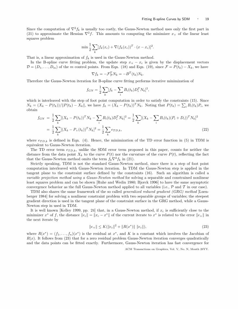
It is well known [Kelley 1999, pp. 24] that, in a Gauss-Newton method, if xc is sufficiently close to theminimizer x∗ of f , the distance ‖ec‖ = ‖xc − x∗‖ of the current iterate to x∗ is related to the error ‖e+‖ inthe next iterate by

‖e+‖ ≤ K(‖ec‖2 + ‖R(x∗)‖ ‖ec‖), (23)

where R(x∗) = (f1, . . . , fn)(x∗) is the residual at x∗, and K is a constant which involves the Jacobian ofR(x). It follows from (23) that for a zero residual problem Gauss-Newton iteration converges quadraticallyand the data points can be fitted exactly. Furthermore, Gauss-Newton iteration has fast convergence for



good initial data and a small residual problem. For a large residual problem, the Gauss-Newton iterationmay not converge at all.

Some variants of the Gauss-Newton method are possible. If only a scalar multiple of the Gauss-Newtonstep, s(x+ − xc), usually with 0 < s < 1, is used for stepping to the next solution, then one obtains thedamped Gauss-Newton method [Kelley 1999].

Another way to modify Gauss-Newton is a regularization with the Levenberg-Marquart method [Kelley1999], in which a scalar multiple of the identity matrix is added to the approximate Hessian. In our setting,this method requires the minimization of

fLM =1

2

∑

k

[(Xk − P+(tk))T Nk]2 + νc

∑

i

||Di||2.

Thus, the regularization term penalizes large changes Di in the control points. It can be shown that usinga regularization parameter νc of the order of the norm of the residual, i.e., O(‖R(xc)‖), one obtains stillquadratic convergence for a zero residual problem. A drawback of the Levenberg-Marquart method in thesetting of curve fitting is that the same magnitude of regularization is applied to every control point, withouttaking into account the curvature variation at different locations.

By writing the fitting error as a function of the parameter values tk, the Levenberg-Marquart method isused in [Sarkar and Menq 1991] to iteratively update the tk, and faster convergence of this method than avariant of PDM is reported. However, although the foot point computation is avoided, it is noted in [Sarkarand Menq 1991] that this variant of the L-M method is about 10 times slower than PDM per iteration.

A global Gauss-Newton method is implemented in [Speer et al. 1998] to update the control points Pi andthe parameter values tk together, therefore avoiding the costly step of computing foot points of data points.However, a relatively large linear system of equations needs to be solved, since now the parameter values of alarge number of data points also enter optimization. The comparison of TDM with this global Gauss-Newtonmethod, as well as other variants of the L-M method, is an interesting problem but beyond the scope of thepresent paper.

6.3 SDM – a quasi-Newton method

In this section we will derive the expression of the Newton method and then reveal the difference betweenour SDM scheme and the Newton method to show that SDM is, in fact, a quasi-Newton method. The keyto this analysis is deriving a suitable expression of the Hessian of the objective function.

For a fixed k, consider the term f2k = FTF . Denote F = (Fx,Fy)

T. By (17), we have ∇f2

k = 2FTPF . The

derivative of ∇f2k yields the Hessian

1

2∇2f2

k = FTPFP + (FT

PF t + FTPtF)∇tT + ∇t(FT

t FP + FTFPt) + (FTttF + FT

t F t)∇t∇tT

+FxF xPP + FyF y PP

= FTPFP + (FT

PF t + FTPtF)∇tT + ∇t(FT

t FP + FTFPt) + (FTttF + FT

t F t)∇t∇tT (24)

Here we used the fact that F xPP = 0,F y PP = 0, since F is linear in P.Again, ∇t stands for the gradient of tk = t(P) with respect to P.On the other hand, we need to find the relationship between ∇t and FP . Differentiating the constraint

(16), we obtain(FT

Pt + ∇tFTtt

)F +

(FT

P + ∇tFTt

)F t = 0. (25)

Solving for ∇t yields

∇t = −FT

PtF + FTPF t

FTttF + FT

t F t.



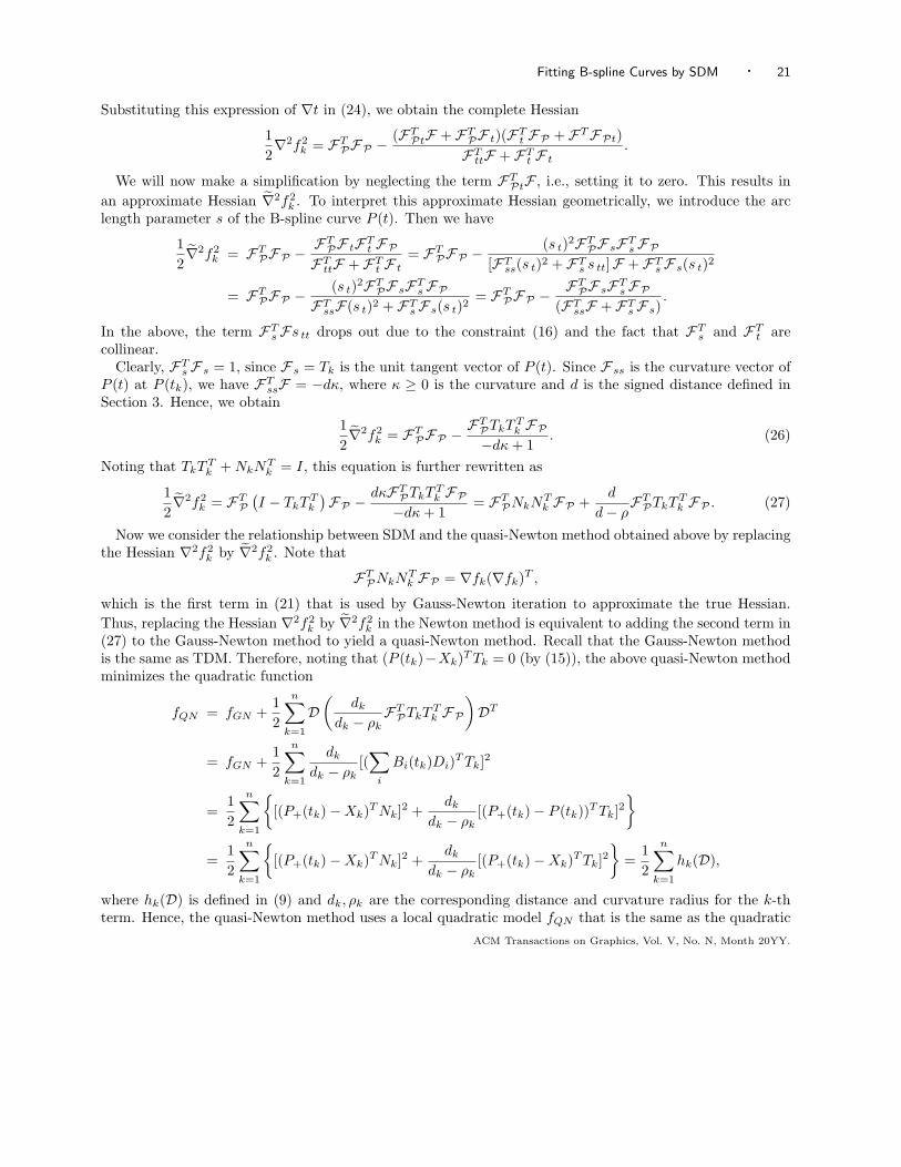
Substituting this expression of ∇t in (24), we obtain the complete Hessian

1

2∇2f2

k = FTPFP −

(FTPtF + FT

PF t)(F

Tt FP + FTFPt)

FTttF + FT

t F t.

We will now make a simplification by neglecting the term FTPtF , i.e., setting it to zero. This results in

an approximate Hessian ∇2f2k . To interpret this approximate Hessian geometrically, we introduce the arc

length parameter s of the B-spline curve P (t). Then we have

1

2∇2f2

k = FTPFP −

FTPF tF

Tt FP

FTttF + FT

t F t= FT

PFP −(s t)

2FTPF sF

Ts FP

[FTss(s t)2 + FT

s s tt]F + FTs F s(s t)2

= FTPFP −

(s t)2FT

PF sF

Ts FP

FTssF(s t)2 + FT

s F s(s t)2= FT

PFP −FT

PF sF

Ts FP

(FTssF + FT

s F s).

In the above, the term FTs Fs tt drops out due to the constraint (16) and the fact that FT

s and FTt are

collinear.Clearly, FT

s F s = 1, since F s = Tk is the unit tangent vector of P (t). Since F ss is the curvature vector ofP (t) at P (tk), we have FT

ssF = −dκ, where κ ≥ 0 is the curvature and d is the signed distance defined inSection 3. Hence, we obtain

1

2∇2f2

k = FTPFP −

FTP

TkTTk FP

−dκ + 1. (26)

Noting that TkTTk + NkNT

k = I, this equation is further rewritten as

1

2∇2f2

k = FTP

(I − TkTT

k

)FP −

dκFTP

TkTTk FP

−dκ + 1= FT

PNkNTk FP +

d

d − ρFT

PTkTTk FP . (27)

Now we consider the relationship between SDM and the quasi-Newton method obtained above by replacingthe Hessian ∇2f2

k by ∇2f2k . Note that

FTPNkNT

k FP = ∇fk(∇fk)T ,

which is the first term in (21) that is used by Gauss-Newton iteration to approximate the true Hessian.

Thus, replacing the Hessian ∇2f2k by ∇2f2

k in the Newton method is equivalent to adding the second term in(27) to the Gauss-Newton method to yield a quasi-Newton method. Recall that the Gauss-Newton methodis the same as TDM. Therefore, noting that (P (tk)−Xk)T Tk = 0 (by (15)), the above quasi-Newton methodminimizes the quadratic function

fQN = fGN +1

2

n∑

k=1

D

(dk

dk − ρkFT

PTkTTk FP

)DT

= fGN +1

2

n∑

k=1

dk

dk − ρk[(∑

i

Bi(tk)Di)T Tk]2

=1

2

n∑

k=1

{[(P+(tk) − Xk)T Nk]2 +

dk

dk − ρk[(P+(tk) − P (tk))T Tk]2

}

=1

2

n∑

k=1

{[(P+(tk) − Xk)T Nk]2 +

dk

dk − ρk[(P+(tk) − Xk)T Tk]2

}=

1

2

n∑

k=1

hk(D),

where hk(D) is defined in (9) and dk, ρk are the corresponding distance and curvature radius for the k-thterm. Hence, the quasi-Newton method uses a local quadratic model fQN that is the same as the quadratic



approximant hk(D) used by the SD error term before it is turned into the semi-definite form in (10). Hence,we have shown that the SDM method is a quasi-Newton method obtained by discarding the term FTFPt,which amounts to disregarding the change FPt of the tangent vector P ′

t (tk) caused by the change of thecontrol points.

SDM does not fall into the category of the quasi-Newton methods that fulfill the so-called secant equation[Kelley 1999]. Instead, SDM uses another positive definite approximant of the Hessian, based on geometricconsiderations. Although SDM is not a standard optimization procedure, it is a computationally attractiveand effective compromise between a full Newton scheme and Gauss-Newton – it picks up more contributionsof the true Hessian than the Gauss-Newton iteration (or TDM) does, but ignores the remaining part forreasons of computational efficiency and simplicity. Indeed, SDM is an optimization scheme that is particularlysuited for solving shape fitting problems, because it uses an intuitively simple error metric that is adaptableto local curvature variation of a target shape.

Each term f2k in the objective function in (14) is the squared distance function. Because the exact Hessian

in the second order Taylor expansion of f2k is modified in order to derive the SD error term, we conclude that,

in general, the SD error term is not a second order approximation to the squared distance, even without themodification in (10) to make the error term positive semi-definite. This is in contrast to the previous squareddistance minimization method by Pottmann et al [Pottmann et al. 2002] where the quadratic approximantin (6) is always a second order approximation to the squared distance function, before the modification toturn it into the positive semi-definite error term in (7).

6.4 Step size control

We have tested step size control on PDM, TDM, and SDM, using the Armijo rule [Kelley 1999]. It is foundthat step size control does not help much with PDM and SDM — PDM still converges slowly, and theper-iteration computation of SDM becomes much longer with moderate degree of improvement in stability.It is found that the stability of TDM improves greatly with the help of step size control, however, at the costof much longer per–iteration time, especially when approaching a local minimum, since, due to the “flat”gradient near a local minimum, it normally gets more time-consuming to select an appropriate step size viarepetitive evaluations of the fitting error.

Figure 17 shows the result of applying step size control (the Armijo rule) to TDM on the same datapoints and initial B-spline curves as shown in Figures 7(a) and 10(a); now both data sets are satisfactorilyapproximated by B-spline curves computed with TDM. For comparison, refer to Figures 7(c) and 10(c) tosee the unacceptable fitting curves generated by TDM without step size control.

P

T

(P0, T0)

Hessian

Fig. 16. The alternating minimization steps of PDMnear a local minimum. P and T stand for the linear

subspaces spanned by the control points and the dataparameters, respectively.

(a) (b)

Fig. 17. TDM using the Armijo rule for step size control. (a)The fitting curve by TDM in 20 iterations for the data set in Fig-

ure 7(a); (b) The fitting curve by TDM in 20 iterations for thedata set in Figure 10(a).



7. CONCLUDING REMARKS

PDM is widely used in practice for parametric curve and surface fitting [Farin 1997]. As we have shown,PDM has linear convergence in theory, converges slowly in practice, and is often trapped in a poor localminimum. TDM is a method often used for curve fitting in computer vision (e.g., [Blake and Isard 1998]).TDM converges faster than PDM, but its convergence is highly unstable. Against this backdrop, we haveproposed a novel and efficient method, called SDM, for fitting B-spline curves to point cloud data. Wehave shown empirically that SDM converges faster than PDM and that SDM is more stable than TDM.In addition, SDM is easy to implement and has similar per-iteration computation time to PDM and TDM,since they share the same framework. All this suggests that SDM is a favorable alternative to PDM or TDMfor B-spline curve fitting.

In order to gain a better understanding of the above geometrically motivated schemes, we have studiedthe B-spline curve fitting problem from the optimization viewpoint. We note that PDM is a gradient descentmethod in a metric that is not well chosen. We have also shown that TDM uses a Gauss-Newton step forsolving a nonlinear least squares problem, and its instability at high curvature regions is thus due to itsomission of important parts in the true Hessian of the objective function and the lack of step size control.Finally, we have shown that our proposed SDM scheme is a quasi-Newton method using a carefully chosenapproximate Hessian, and thus its superior performance in both convergence and stability does not comeas a surprise. Interestingly, unlike most other quasi-Newton methods, the approximate Hessian used bySDM is not explicitly computed; it arises naturally as the consequence of using the simple SDM error termdevised out of entirely geometric considerations, i.e., making use of curvature information to give a closeapproximation of the squared distance function. This contributes to the simplicity and efficiency of SDM.

We expect to see more studies on SDM and related problems, both theoretically and from the viewpoint ofapplications. An immediate extension is to apply SDM to optimize the weights and knots of a NURBS fittingcurve, an issued discussed in [Laurent-Gengoux and Mekhilef 1993; Goldenthal and Bercovier 2004]. Othersignificant problems include the analysis of the convergence rate of SDM and the improvement of the globalconvergence to the target shape from a very simple “seed” shape; the latter topic has a close connection tothe work on active contours [Kass et al. 1988; Malladi et al. 1995; Osher and Fedkiw 2003; Sethian 1999].

Our ongoing research shows that SDM can be applied to a large class of shape reconstruction and geo-metric optimization problems, such as fitting B-spline surfaces or subdivision surfaces, optimization over ananalytical surface or a mesh surface, and surface registration. This extension of SDM to the surface casewould be of great practical importance, in view of the current use of PDM as a predominant optimizationmethod for surface fitting in graphics and CAD.

REFERENCES

Ambrosio, L. and Montegazza, C. 1998. Curvature and distance function from a manifold. Journal of Geometric Analysis 8,

723–748.

Bercovier, M. and Jacob, M. 1994. Minimization, constraints and composite bezier curves. Computer Aided Geometric

Design 11, 533–563.

Bjorck, A. 1996. Numerical Methods for Least Squares Problems. Mathematics Society for Industrial and Applied Mathe-

matics, Philadelphia.

Blake, A. and Isard, M. 1998. Active Contours. Springer, New York.

Djebali, M., Melkemi, M., and Sapidis, N. 2002. Range-image segmentation and model reconstruction based on a fit-and-

merge strategy. In Proceedings of the Seventh ACM Symposium on Solid Modeling and Applications. 127–138.

Farin, G. 1997. Curves and Surfaces for Computer Aided Geometric Design: A Practical Guide, 4th ed. Academic Press,

New York.

Forsey, D. R. and Bartels, R. H. 1995. Surface fitting with hierarchical splines. ACM Transactions on Graphics 14, 134–161.

Goldenthal, R. and Bercovier, M. 2004. Spline curve approximation and design by optimal control over the knots. Com-puting 72, 53–64.



Goshtasby, A. A. 2000. Grouping and parameterizing irregularly spaced points for curve fitting. ACM Transactions onGraphics 19, 185–203.

Greiner, G., Kolb, A., and Riepl, A. 2002. Scattered data interpolation using data dependant optimization techniques.Graphical Models 64, 1–18.

Haber, J., Zeilfelder, F., Davydov, O., and Seidel, H. P. 2001. Smooth approximation and rendering of large scattereddata sets. In Proceedings of Visualization’01. 341–348.

Hoppe, H. 1996. Progressive meshes. In Proceedings of SIGGRAPH’96. 99–108.

Hoppe, H., DeRose, T., Duchamp, T., Halstead, M., Jin, H., McDonald, J., Schweitzer, J., and Stuetzle, W. 1994.Piecewise smooth surface reconstruction. In Proceedings of SIGGRAPH’94. 295–302.

Hoschek, J. 1988. Intrinsic parameterization for approximation. Computer Aided Geometric Design 5, 27–31.

Hoschek, J. and Lasser, D. 1993. Fundamentals of Computer Aided Geometric Design. AK Peters.

Hu, S. M. and Wallner, J. 2005. second order algorithm for orthogonal projection onto curves and surfaces. Computer AidedGeometric Design 22, 251–260.

Kass, M., Witkin, A., and Terzopoulos, D. 1988. Snakes: active contour models. International Journal of ComputerVision 1, 321–331.

Kelley, C. T. 1999. Iterative Methods for Optimization. Society for Industrial and Applied Mathematics, Philadelphia.

Laurent-Gengoux, P. and Mekhilef, M. 1993. Optimization of a nurbs representation. Computer-aided Design 25, 699–710.

Lee, E. T. Y. 1989. Choosing nodes in parametric curve interpolation. Computer-aided Design 21, 363–370.

Luenberger, D. 1984. Linear and Nonlinear Programming. Addision-Wesley.

Ma, W. Y. and Kruth, J. P. 1995. Parameterization of randomly measured points for least squares fitting of b-spline curvesand surfaces. Computer-aided Design 27, 663–675.

Maekawa, I. and Ko, K. 2002. Surface construction by fitting unorganized curves. Graphical Models 64, 316–332.

Malladi, R., Sethian, J., and Vemuri, B. C. 1995. Shape modeling with front propagation: A level set approach. IEEE

Transactions on Pattern Analysis and Machine Intelligence 17, 158–175.

Osher, S. and Fedkiw. 2003. Level Set Methods and Dynamic Implicit Surfaces. Springer-Verlag, New York.

Pavlidis, T. 1983. Curve fitting with conic splines. ACM Transactions on Graphics 2, 1–31.

Plass, M. and Stone, M. 1983. Curve-fitting with piecewise parametric cubics. Computer Graphics 17, 3, 229–239.

Pottmann, H. and Hofer, M. 2003. Geometry of the squared distance function to curves and surfaces. In Visualization andMathematics III, H. Hege and K. Polthier, Eds. 223–244.

Pottmann, H., Leopoldseder, S., and Hofer, M. 2002. Approximation with active b-spline curves and surfaces. In Pro-ceedings of Pacific Graphics 2002. IEEE Computer Society Press, 8–25.

Pottmann, H. and Wallner, J. 2001. Computational Line Geometry. Springer-Verlag, Berlin.

Pratt, V. 1985. Techniques for conic splines. In Proceedings of SIGGRAPH’85. 151–160.

Ruhe, A. and Wedin, P. 1980. Algorithms for separable nonlinear least squares problems. SIAM Review 22, 318–337.

Sarkar, B. and Menq, C.-H. 1991. Parameter optimization in approximating curves and surfaces to measurement data.

Computer Aided Geometric Design 8, 267–290.

Saux, E. and Daniel, M. 2003. An improved hoschek intrinsic parametrization. Computer Aided Geometric Design 20,

513–521.

Sethian, J. A. 1999. Level Set Methods and Fast Marching Methods. Cambridge University Press.

Speer, T., Kuppe, M., and Hoschek, J. 1998. Global reparameterization for curve approximation. Computer Aided GeometricDesign 15, 869–877.

Taubin, G. 2002. Dual mesh resampling. Graphical Models 64, 94–113.

Walton, D. J. and Xu, R. 1991. Turning point preserving planar interpolation. ACM Transactions on Graphics 10, 297 –

311.

Wang, X. C. and Phillips, C. 2002. Multi-weight enveloping: least-squares approximation techniques for skin animation. In

Proceedings of the 2002 ACM SIGGRAPH/Eurographics Symposium on Computer animation. 129 – 138.

Weiss, V., Andor, L., Renner, G., and Varady, T. 2002. Advanced surface fitting techniques. Computer Aided GeometricDesign 19, 19–42.

Yang, H. P., Wang, W., and Sun, J. G. 2004. Control point adjustment for b-spline curve approximation. Computer-aidedDesign 36, 639–652.


Fitting B-spline Curves to Point Clouds by Curvature-Based ... · by Curvature-Based Squared...

Documents

Transcript of Fitting B-spline Curves to Point Clouds by Curvature-Based ... · by Curvature-Based Squared...