Governors State UniversityOPUS Open Portal to University Scholarship

All Student Theses Student Theses

Summer 2017

Fitting a Linear Regression Model and Forecastingin R in the Presence of Heteroskedascity withParticular Reference to Advanced RegressionTechnique Dataset on kaggle.com.Samuel Mbah NdeGovernors State University

Follow this and additional works at: http://opus.govst.edu/theses

Part of the Numerical Analysis and Computation Commons

For more information about the academic degree, extended learning, and certificate programs of Governors State University, go tohttp://www.govst.edu/Academics/Degree_Programs_and_Certifications/

Visit the Governors State Mathematics DepartmentThis Thesis is brought to you for free and open access by the Student Theses at OPUS Open Portal to University Scholarship. It has been accepted forinclusion in All Student Theses by an authorized administrator of OPUS Open Portal to University Scholarship. For more information, please contactopus@govst.edu.

Recommended CitationNde, Samuel Mbah, "Fitting a Linear Regression Model and Forecasting in R in the Presence of Heteroskedascity with ParticularReference to Advanced Regression Technique Dataset on kaggle.com." (2017). All Student Theses. 99.http://opus.govst.edu/theses/99

Fitting a Linear Regression Model and Forecasting in R in the Presence of Heteroskedascity

with Particular Reference to Advanced Regression Technique Dataset on kaggle.com.

By

Nde, Samuel Mbah

BSc. Mathematics and Statistics, University of Bamenda, 2014.

Bed. Mathematics, University of Bamenda, 2013.

Thesis

Submitted in partial fulfillment of the requirements

For the Degree of Master of Science,

With a Major in Mathematics.

Governors State University

University Park, IL 60484.

2017

i

ABSTRACT

Since ancient times, men have built and sold houses. But just how much is a house worth?

The challenge is to be able to use information about a house such as its location, and the

area on which it is built to predict its price. Such predicted prices can be of great

importance to any participant in the real estate business be it an agent, a buyer, seller or a

bank to make intelligent decisions and the profit that come with such decisions. Since every

company’s success depends on its ability to accurately predict financial outcomes, its

profitability will depend on how well it can forecast economic outcomes. The goal of this

thesis is to demonstrate how to use the forecasting tools of the software R to forecast house

prices. To achieve this, we use random forest, correlation plots and scatter plots to select

variables to include to use in building a model using the information in one of the data sets

(training data set) and then test the effectiveness of the model on another set (test data

set). Then, we explore the relationships between these variables and decide whether it is

appropriate to build linear models(lm) or a generalized linear models(glm). Finally, we

build our model on the dataset making sure to avoid an overly complex or overfit model.

Noting that our model suffers from unconditional heteroskedasticity, we discuss its

goodness of fit. Then we use the model to predict sales prices for the point in the testing

data set.

Key Words: Forecasting, Training, Testing, Linear Model, Overfit, Heteroskedasticity,

Goodness of Fit.

ii

Dedication This work is dedicated to Mr. Albert Cox and his wife Mrs. Joyce Ache for their continual

support and encouragement. Special thanks to statistics community on YouTube and the R

bloggers on StackOverflow. I could not have done much without you.

iii

Contents ABSTRACT ................................................................................................................................................... i

Dedication ................................................................................................................................................................ ii

List of Tables ........................................................................................................................................................... v

List of Figures ........................................................................................................................................................ vi

CHAPTER 1 .............................................................................................................................................................. 1

INTRODUCTION ......................................................................................................................................... 1

1.1 Problem Statement ......................................................................................................................... 1

1.2 Goal Of this Thesis ........................................................................................................................... 2

1.3 Outline of the Thesis. ...................................................................................................................... 3

CHAPTER 2 .............................................................................................................................................................. 5

NATURE AND USES OF FORECASTS ........................................................................................................... 5

2.1 Why Should We Forecast? .............................................................................................................. 6

2.2 What is Regression? ........................................................................................................................ 8

2.3 What is Multiple Linear Regression? ............................................................................................ 10

2.4 Assumptions of a Linear Regression Model. ................................................................................. 12

2.5 How do we select the variables to include in our model? ............................................................ 13

2.5.1 Selecting variables using Correlation Plots ............................................................................ 14

2.5.2 Selecting Variables using Random Forest. ............................................................................. 17

2.5.3 Selecting Variables using the “glmulti” function. .................................................................. 19

CHAPTER THREE ............................................................................................................................................... 23

DETECTING AND FIXING PROBLEMS ASSOCIATED WITH LINEAR REGRESSION MODELS ....................... 23

3.1 What is Cross Validation? ............................................................................................................. 23

3.2 Different Methods of Cross Validation ......................................................................................... 24

3.3 The Problem of Heteroskedascity ................................................................................................. 26

3.4 Tests for Heteroskedasticity ......................................................................................................... 28

3.5 The Problem of Overfitting and Underfitting................................................................................ 31

iv

3.6 Interpreting Linear Model Results ................................................................................................ 34

3.7 Interpreting Diagnostic plots for Linear Regression Models. ....................................................... 37

CHAPTER FOUR .................................................................................................................................................. 42

METHOD. ................................................................................................................................................. 42

4.1 A quick look at the data. ............................................................................................................... 42

4.2 How do we Handle Missing Values and Typos (data cleaning)? ................................................... 42

4.3 How to Select the variables to Include in the Model .................................................................... 43

4.3.1 How to use Correlation Plots to Select the variables to include in a model. ......................... 44

4.3.2 How to use “glmulti” to select variables to include in a model. ............................................ 49

4.3.3 How to use Random Forest to select variables to include in a model. .................................. 51

4.4 Building and Discussing Model1 ................................................................................................... 53

4.6 Building and Discussing Model3 ................................................................................................... 65

CHAPTER 5 ........................................................................................................................................................... 73

USING THE MODEL .................................................................................................................................. 73

CHAPTER 6 ........................................................................................................................................................... 76

FINDINGS AND CONCLUSION .................................................................................................................. 76

REFERENCES ....................................................................................................................................................... 80

References ............................................................................................................................................................ 80

v

List of Tables

Table 1: Summary of all three models. ...................................................................................................... 71

Table 2: Ranking of variables by their importance. .............................................................................. 78

vi

List of Figures

Figure 2.1: glmulti displaying different models and their support ................................................ 20

Figure 2.2 Correlation Plot for all the variables in my data frame. ................................................ 16

Figure 2.3: Correlation plot for some of the variables in my dataset ........ Error! Bookmark not

defined.

Figure 3.1: Plots displaying heteroskedastic and homoscedastic trends .................................... 27

Figure 3.2: Overfitting and Underfitting. .................................................................................................. 32

Figure 4.1: Variable Importance Plot Using Random Forest ............................................................. 52

Figure 4.2: Correlation Plot ............................................................................................................................ 45

Figure 4.3 (a)Correlation plot of the first 21 variables ....................................................................... 46

Figure 4.3 (b) Correlation plot of the second 21 variables................................................................ 47

Figure 4.3 (c) Correlation plot of the third 21 variables .................................................................... 48

Figure 4.3 (d) Correlation plot of the last 21 variables ...................................................................... 49

Figure 4.4 Correlation plot variables that are highly correlated with SalePrice ....................... 54

Figure 4.5: Residual analysis plots of the results of model1. ....... Error! Bookmark not defined.

Figure 4.6: Correlation Plot for the variables in model1 .................................................................... 61

Figure 4.7Correlation plot for the variables in model2 ...................................................................... 62

Figure 4.8: Plot summary of model2 .......................................................................................................... 64

Figure 4.9 (a) SalePrice vs Other variables of Model3 ........................................................................ 67

vii

Figure 4.9 (b) SalePrice vs Other variables of Model3 ........................................................................ 67

Figure 4.9 (c) SalePrice vs Other variables of Model3 ................... Error! Bookmark not defined.

Figure 4.10 Plot of model3. ............................................................................................................................ 70

1

CHAPTER 1

INTRODUCTION

Housing is one to the biggest problems of modern society. Almost every adult must at some

point decide whether to buy a house or to pay rents. But with the society becoming

increasingly complex, resources becoming scarcer, and construction cost skyrocketing,

almost everything from the location, size, year built etc. to government policies and social

amenities like parks and libraries have had to influence the value of real estate. In general,

the factors that influence the value of real estate can be grouped into economic, social,

governmental and physical/environmental (Carr, Lawson, & Schultz, 2010).

1.1 Problem Statement

Many banks, real estate agents and individuals often need to valuate a home before giving

out a loan, buying or selling it. Even the government is interested in knowing how much

every home is worth for taxation purposes. Other businesses need to know just how much

they should put for a new location or to extend their parking lot. In all these instances, a

good forecast of the best price of the property in question would be a pricy piece of jewelry.

However, getting such a forecast might not be possible because of the following reasons

discussed in (Fawumi, 2015);

• Unavailability of skilled analyst to perform detailed analysis

• Need for frequent updates to the analyses

• Large amount of data to be handled for every property

• Need to discover and understand the appropriate statistical models for analysis.

2

Because every individual’s knowledge and experience is limited to a certain level their

ability to analyze any given data will still be limited. As of now, such data tasks are

performed by technical experts, professional statisticians, data analysts etc. using advanced

methodologies which might not be comprehensible to the lay man. Thus, many institutions

pay highly for professionals and tools to manage and analyze their data, a cost that is even

higher for real estate dealer that must frequently call for expert services. It is amidst these

difficulties that the goal of this thesis arises.

1.2 Goal Of this Thesis

The goal of this thesis is to use the free software R to design code that can be used by

individuals and/or businesses having data pertaining to real estate to predict house prices

by fitting a linear regression line to the data. To achieve this goal, this thesis aims to answer

the following questions.

• What is linear regression? When and how should it be used?

• How do we fill missing values (empty and/or incorrectly filled cells) in a data set?

• What variables should we use in our linear regression model and why? What causes

Heteroskedasticity and how can it be fixed?

• What techniques can we use to verify whether a model is a good fit to the data?

• How do we predict a variable from other variables in a data set (data frame) in R?

I answer the above questions in this thesis as described in the following outline.

3

1.3 Outline of the Thesis.

To answer the questions asked above and meet the stated goal, this thesis has been

arranged in the following order.

Chapter one is the introduction in which I have stated the problem and objective and asked

the questions that I intent to answer in the rest of this document. It also includes a brief

description of all the steps that I intend to go through to answer the questions I have asked

and meet the stated goal.

Chapter two starts with the nature of forecasting and the reasons for forecasting. It

contains a theoretical background in which we discuss linear regression. Though we briefly

mention other types of regression analysis, such as generalized linear regression, its focus

linear regression. Here, we discuss how to choose the variables to include in our model and

how to build the model in R.

Chapter three focuses on the results of the linear regression model. Here, we talk about the

problems associated with linear regression models and how to fix them. Specifically, we

talk about the problems of heteroskedasticity and overfitting – how to detect and fix these

problems. In statistical terms, we may say chapter three is about cross validating the

model.

In chapter four, we put together all the ideas discussed in the first three chapters. Here,

using the Advanced Regression Technique Dataset on kaggle.com, we explore the data set

to see if there are any missing values and if there are, we fill them. Then, we use correlation

plots and random forest as well as scatter plots to select the variables to include in our

linear model. Then we build various models and using cross validation techniques, some

4

variables are scaled out till we get the best model. This chapter contains a lot of graphs and

the interpretation of the results from the model we build. It is the chapter for those who are

interested in the coding and testing of hypotheses about linear regression models.

Chapter five discusses the results of the predicted sales prices for the test data set.

Chapter six gives the conclusion and discusses other possible softwares that could be used

for the data set. Finally, the R-code I made for this thesis is attached at the appendix.

5

CHAPTER 2

NATURE AND USES OF FORECASTS

According to BusinessDictionary.com, a forecast is “a planning tool that helps management

in its attempts to cope with the uncertainty of the future, relying mainly on data from the

past and present and analysis of trends” (IAC, 2017). Dealing with data is usually not an

easy task, especially when using the data to predict the future. One reason why forecasts

are so difficult to make is that they are based on historical data and trend and the forecasts

are usually made with the hope that those past trends will reoccur in the future. However,

this is not usually the case. Forecasts are even worsened by the fact that they usually

involve human behavior which is subject to change. The famous scientist Isaac Newton

learnt this the hard way. After losing £20,000 (more than $3,000,000 in 2003 dollars) in his

South Sea shares, he lamented “I can calculate the motion of heavenly bodies, but not the

madness of people.” Paul Lemberg emphasizes this in his article Why Predict the Future?

when he says;

“Predicting the future is hard. It’s so hard that a 50% success rate is considered

extraordinary for a professional futurist. In other words, the professionals are wrong at

least half of the time. Yet we need these predictions; we need to make plans.” (Lemberg,

2001)

Because of the importance of forecasting, it has found its way into many fields of studies

and is being applied in almost every industry. In the finance industry, actuaries are using

forecasts to determine insurance premiums. In environmental science, forecasts are being

used daily to tell what the weather would be. Politicians are using forecasts to determine

6

their chances of success in an election and to improve their strategies. As these examples

have indicated, almost all forecasts are related to planning for the future and this is only

natural because failing to plan is planning to fail.

According to (Montgomery, 2008, pp. 2-3), forecasting problems can be classified into

three groups - short, medium and long terms. Short term forecasts such as weather

forecasts are those that deal with events or processes that last for minutes, hours, days or

weeks. Medium term forecasting problems deal with forecasts that last for one or two year.

Long term forecasts usually require a lot of effort and are related to making big decisions.

An example of a long-term forecasting problem would be forecasting the number of barrels

of oil that would be used in the United States in the year 2030.

2.1 Why Should We Forecast?

Knowledge of the future is the one sure way to having a bright future. To forecast means to

have knowledge about the future and this can be very helpful to individuals and businesses.

To illustrate how forecasts can be helpful to a company, let us consider a company called

PostCards that produces post cards. By analyzing past sales data, the marketing

department of PostCards might note that there is a high demand for her products during

the festive months of February (valentine’s day), November (Thanksgiving Day) and

December (end of year festivals). She (PostCards) might then use this information in the

following ways.

1. Operations Management. PostCards’ management will be aware that there shall be a

higher demand during the festive months and thus schedule for the production and

distribution of more cards during those months.

7

2. Marketing. Since the analysis of past transaction data reveals that there shall be more

demand for her products during the festive month, the marketing department of PostCards

will push for more advertisements during that time. They might even organize seasonal

sales and other promotions to boost their sales. They might even need to hire more sales

staff or allow overtime for the marketers.

3. Finance and Risk Management. Forecasts can also be used for risk management and

financial planning. Since investors in PostCards are interested in how much return they can

get from their investment, they could use the forecasts of PostCards future sales to

determine whether the potential sales would meet the level of returns that they seek from

their investments. PostCard’s management may also use such information to determine

how much to spend on research and what salaries workers should be paid.

4. Economics. Forecasts of future sales would help the human resource department of

PostCards to determine how many workers would be needed to produce as enough goods

to meet the forecasted future demand. This will also help that company evaluate its growth

and set production targets.

5. Industrial Process Control. Forecasts of the future sales would influence the type of

production process the company would choose. In the case of PostCards, forecast of future

sales can influence the production process as follows. If historical data proves that 2 out of

every 100 postcards made are of a low quality and cannot be sold, and suppose PostCards

has forecasted that 10000 postcards would be needed for a certain period, then, she would

have to manufacture 10203 postcards to meet the forecasted demand. This is because it

8

would be expected that 203 postcards would not meet the quality requirements for a

postcard to be sold.

6. Demography. Understanding demography can be very important for a business in

determining where and how to distribute her products. Knowing where the demand for the

products is high will help the business determine how much quantity of goods to go to

every shopping center. For the PostCards company that we have been talking about, if they

discover that a high demand for their products comes from the city centers, it will be logical

for management to arrange for more cards to be sent to the city centers. They might even

want to consider a post card shop in areas of great demand.

2.2 What is Regression?

Regression is a statistical process for estimating relationship between two or more

variables. Regression can be linear or nonlinear. In linear regression, the relationship is

modeled by functions which are linear combinations of variable. In nonlinear regression,

the relationship is modeled by functions of nonlinear combinations of variables. In

regression, we generally use one or more variables to predict another variable. The

simplest form of regression involves two variables, the explanatory or independent

variable (usually denoted 𝑋) which is used to predict another variable called the response

or dependent variable (usually denoted 𝑌). Thus, the simplest regression problem involves

two variables, the variable that is being predicted(𝑌) which serves as a response from the

model (reason why it is called the response variable) and the explanatory variable (𝑋) that

9

explains the prediction (reason why it is called the explanatory variable). In this case, we

assume that the explanatory variable (𝑋) and a response variable (𝑌), are related by;

𝑌 = 𝛽0 + 𝛽1𝑋 + 𝜀

where 𝛽0 and 𝛽1 are unknown model parameters which we must estimate and ε is an error

term which cannot be modeled. Here, 𝛽0 gives the Y- intercept and 𝛽1 gives the slope and

direction of the regression line. To estimate these parameters, we leave out the error term

(since it cannot be modeled) and model the relationship by;

Ŷ = 𝑏0 + 𝑏1𝑋

Where Ŷ is the predicted or theoretical value given by the model, 𝑏0 and 𝑏1 are estimates of

𝛽0 and 𝛽1 respectively. The residual 𝑒 shows the difference between the observed and the

predicted value of the model. It is calculated as follows

𝑅𝑒𝑠𝑖𝑑𝑢𝑎𝑙 = 𝑒 = 𝑌 − Ŷ = 𝑌 − (𝑏0 + 𝑏1𝑋).

The regression coefficient (𝑅2) shows how well the values fit the data, that is how much of

the variation in Y is explained by model Ŷ = 𝑏0 + 𝑏1𝑋.

This means that regression can tell us how much change we should expect in one variable if

we change the other by a certain amount. However, what causes the change is not known.

This means that regression does not show us causation. To illustrate, suppose one does a

regression on the prices of houses in a neighborhood against the salaries of the home

owners, the regression analysis will give a high positive coefficient of correlation but this is

not to say high salaries cause high home prices. The high correlation coefficient and the

total lack of causation speaks to the fact that correlation is involved in determining the

10

strength of the relationship between two variables by quantifying the association while

regression is more concern with explaining how much change one to expect in one variable

when the other changes by a given amount.

It is very important to understand the difference between correlation and regression

analysis. Regression attempts to identify the relationship between two or more variables

while correlation determines the strength of the relationship between two variables. (see

(Hood & Green, 2006))

Since no single straight line can pass through all the data points in most real-world

situations (as is the case with the data set I use for this thesis), we tend to find the line that

best fits our data set. Such a line is called the line of “best fit”. The Ordinary Least Squares

(OLS) regression procedure will compute the values of the parameters 𝑏0 and 𝑏1

(respectively the intercept and slope of the regression line) that best fit the observations.

The vertical distance between each observation and the line of “best fit”—the regression

line—is called the residual. To learn more about how ordinary least squares are derived,

see (Benoit, 2010).

2.3 What is Multiple Linear Regression?

Multiple linear regression is used to model situations where the response variable is

linearly dependent on more than one explanatory variable. Suppose we have four

explanatory 𝑋1, 𝑋2, 𝑋3, and 𝑋4, variables and one response variable Y, the observed process

would be;

𝑌 = 𝛽0 + 𝛽1𝑋1 + 𝛽2𝑋2 + 𝛽3𝑋3 + 𝛽4𝑋4 + 𝜀 = 𝛽0 + ∑ 𝛽𝑗 𝑋𝑗

4

𝑗=1

+ 𝜀

11

which we can model by;

Ŷ = 𝑏0 + 𝑏1𝑋1 + 𝑏2𝑋2 + 𝑏3𝑋3 + 𝑏4𝑋4 = 𝑏0 + ∑ 𝑏𝑗 𝑋𝑗

4

𝑗=1

where 𝑏0 and ε are the slope and error terms and the 𝑏𝑗′𝑠, 𝑗 ∊ 1. .4 are the estimated

coefficients of the 𝑋𝑗′𝑠, 𝑗 ∊ 1. .4. The equation displayed above is the multiple linear

regression equation when we have 4 explanatory variables. The generalized multiple linear

regression is given by;

Ŷ = 𝑏0 + 𝑏1𝑋1 + 𝑏2𝑋2 + ⋯ + 𝑏𝑛𝑋𝑛 = 𝑏0 + ∑ 𝑏𝑗 𝑋𝑗

𝑛

𝑗=1

where like before, 𝑏0 is the intercept, ε is the error term and the 𝑏𝑗′𝑠, 𝑗 ∊ 1. . 𝑛 are the

coefficients of the 𝑛 independent variables 𝑋𝑗′𝑠, 𝑗 ∊ 1. . 𝑛. The residuals would be calculated

by;

𝑒𝑖 = 𝑌𝑖 − Ŷ𝑖 = 𝑌 − (𝑏0 + 𝑏1𝑋1 + 𝑏2𝑋2 + ⋯ + 𝑏𝑛𝑋𝑛)

where 𝑌𝑖 is the actual or observed value of the response value and Ŷ𝑖 is the fitted value in

the 𝑖𝑡ℎ instance (𝑖 ∈ 1. . 𝑁 where 𝑁 is the number of data points in the data set). In multiple

linear regression, we fit a linear relationship between independent variables and the

dependent variable. However, the slope and coefficients cannot be interpreted as those of

the simple linear model of Ŷ = 𝑏0 + 𝑏1𝑋 with one intercept 𝑏0 and one slope 𝑏1. The

coefficients 𝑏𝑗, 𝑗 ∊ 1. . 𝑛 could be viewed as the link relating every 𝑋𝑗, 𝑗 ∊ 1. . 𝑛 to 𝑌. We have

made mention of the fact that we use ordinary least squared (OLS) procedure to estimate

the parameters 𝑏𝑗′𝑠 but our choice for this procedure is not for nothing. For one thing, OLS

has some very nice mathematical properties, for example it presents a function that can be

12

differentiated and its errors are normally distributed errors. For more information on

ordinary least squares, see (Giordano, Fox, & Horton, 2015, pp. 121-128). These are

desirable characteristics, however, to apply ordinary least squares technique, certain

conditions must be met.

2.4 Assumptions of a Linear Regression Model.

Certain criteria must be met to build a linear regression model based on ordinary least

squares technique. These assumptions are outlined in (Dan Campbell, 2008, p. 6) together

with the penalties and discussed below;

1. The proposed linear model is the correct model. This means that the technique may not

produce its best estimates of the parameters 𝛽𝑗 , 𝑗 ∊ 0. . 𝑛 if the model is misspecified. We

can misspecify the model by not including (a) variable(s) that are highly related to the

independent variable. For example, modelling the frequency of a pendulum without

using its length.

2. The mean of the error term should be independent of the observed dependent

variables. If this is not the case, it would likely be the case that at least a variable is

missing and in the model and is being represented by the errors.

3. The error terms are uncorrelated with each other and exhibit constant variance that

does not depend on the observed X variables i.e. 𝑉𝑎𝑟(𝑌𝑖|𝑋𝑖) = 𝜎2 (homoskedasticity).

Violating this requirement would lead to a situation where the error terms are related

to the independent variables (heteroskedasticity) i.e. 𝑉𝑎𝑟(𝑌𝑖|𝑋𝑖) = 𝜎𝑖2. This often

shows itself by trends in the scatter plots of the residuals.

13

4. No independent variable exactly predicts another. When an independent variable

predicts another independent variable in a model, the model would be adding extra

weight to the variable. It would be as though the variable were used in the model twice.

One could violate this requirement by for example putting the age of a person and the

date he/she was born in the same model.

If the four assumptions listed above are met, then the Gauss-Markov Theorem states that

the Ordinary Least Squares regression estimator of the coefficients of the model is the Best

Linear Unbiased Estimator (BLUE) of the effect of X on Y. Essentially this means that it is

the most accurate estimate of the effect of X on Y. See (Flinn, 2004) for a proof of the Gauss-

Markov Theorem.

2.5 How do we select the variables to include in our model?

In our discussion, thus far, we have assumed that the response variables in our model are

known. But just how exactly are these variables selected? The fourth assumption for

building a linear model (Dan Campbell, 2008, p. 6) listed above is very helpful in choosing

which variable to include in our model. According to this assumption, none of the

independent variables should exactly predict the other. Though we may have all the

variables in our data frame standing right in front of us, it might not be easy to tell which

variable predicts the other. Traditionally, one would have to use their knowledge and

experience to choose the best variables one feels would be appropriate for the model but as

but this method would become useless when one has a very large set of data with

thousands of variables. Many techniques including correlation plots and random forests

have proven to be very helpful in solving this problem.

14

2.5.1 Selecting variables using Correlation Plots

Correlation plots can be used in selecting variables to include in Model. This method uses

the idea that the ‘best’ model should be one with explanatory variables that are highly

correlated with the response variable. This is true because variables that exactly predict

each other will have a high correlation and would violate the assumption of independence

of variables to include in a linear model. Thus, a correlation plot that displays graphically,

the correlations among the various variables can be used to select the variables that are

highly correlated with the response variable and not so well correlated amongst

themselves to include in the model.

Though this method is very good for small data set, it becomes a problem understanding a

correlation matrix for data sets with large number of variables. Note that one can only get a

correlation plot for data that is numerical. Thus, one must convert all the categorical

variables to numerical variables before doing a correlation plot. Correlation plots do not

produce good results with categorical variables because each category is treated as

separate variable with unknown values where the category is missing. For example, if a

dataset consists one 100 points and a categorical variable in that dataset has 5 levels of 20

points each, then, upon converting the variable to a numerical variable, we would have 5

variables each having 80 zeroes. The new variables created are called dummy variables.

Note that categorical variables are actually converted to a numerical code. For example, the

categorical variable Gender with two levels Male and Female could be converted to a

numerical variable by creating two new variables (GenderMale and GenderFemale, say)

GenderMale would have ones to those points that were male in gender and zeroes for every

other point. Similarly, GenderFemale would have 1 for those points that were female in

15

gender and zeroes for every other point. This means that a dummy variable can take only

one of two possibilities, 0 or 1. The creation of dummy variables during the conversion

process results in lower correlations for categorical variables. For this reason, we rely more

on random forests to select the categorical variables to include in the model. Below is a

correlation plot for all the variables in the data set that I am using for this thesis.

Figure 2.1: The correlation plot for all the variables in my data frame

16

Figure 2.2 Correlation Plot for some of the variables in the dataset.

The first correlation plot (figure 2.1) shows the correlations of all the variables in the data

set. It shows us just how messy a correlation plot might become when the number of

variables is too large. The second correlation plot above (figure 2.2) indicates to us just

how good a correlation plot with the right number of variable may be.

One thing to keep in mind about correlation plots is that all the correlations on the leading

diagonal must be one. This is because every variable is perfectly correlated with itself. The

color column on the right of each plot shows the level of correlation. It is some form of scale

17

that tells us how much correlation there is between any given two variables. Also, notice

that the correlation matrix is symmetric about the leading diagonal. This is so because

every variable on the horizontal axis is also on the vertical axis.

Since we are interested in knowing the correlations between the dependent variable and

every other variable in our data set, we will always concentrate on the column or row that

that contains the dependent variable. To select the variables to include in our model, we

must set a minimum require correlation level. For example, if we set the minimum required

correlation level to 70% (𝑖𝑒 |𝑟| ≥ 0.7) then all variables whose correlation with our

dependent variable is at least 0.7 would be included in the first model that we build. But

this does not mean that these variables must be in the model. We might do a correlation

matrix on these variable and find that some of them are highly correlated. In such a case,

we must remove one variable in every pair of highly correlated variables.

2.5.2 Selecting Variables using Random Forest.

Random forests can be used for regression. The random algorithm works by fitting a

regression model to the response variable using one explanatory variable at a time. The

mean square error of the predictions of each model (and therefore each explanatory

variable) is calculated. Mean square error is calculated by;

𝑀𝑆𝐸 =∑ (Y − Ŷ)

2 𝑁

1

𝑁

where N is the number of data points in the dataset. The data set is then split into several

subsets and the sum of square errors on each subset is calculated (the sum of square errors

is calculated on each subset by 𝑆𝑆𝐸 = ∑(𝑌 − Ŷ)2

). On each of the subsets, the variable with

18

the smallest 𝑆𝑆𝐸 is counted as a node for that variable. The total number of nodes for each

variable is counted. The total count of the nodes for each variable would be its node purity.

The variable with the highest number of nodes is the most important predictor judging by

the “IncNodePurity”.

In R, it is imperative to install the random forest package (“randomForest”) and load its

library to be able to access the algorithm. We must also specify the target variables and

data set before running the algorithm. The results of the algorithm can be displayed

through a variable importance plot (“varImpPlot”) which orders the explanatory variables

in order of decreasing predictive ability of the response variable. When using this method,

the importance of the variables can be given in two ways – using a percentage mean square

error contribution (“%incMSE”) or a node purity (“IncNodePurity”). The “%incMSE” of a

variable is the increase in predictive power of a model as that results from randomly

changing its value (if it is a numerical variable) or category (if it is a categorical variable) of

the variable. It is calculated using the mean square error of prediction. The IncNodePurity

of a variable refers how well the explanatory variable performs on the several splits of the

data.

In addition to being time saving, random forests have the extra advantage that they can

handle missing values. If a variable is categorical, a new category for the missing data is

introduced. The case of numerical variables is quite different. The algorithm weighs the

neighboring points and assigns a value to the target missing point (Hastie, Tibshirani, &

Friedman, 2008, pp. 616-620). For more information on the use of random forests for

variable selection, see (Breiman & Cutler, 2004).

19

2.5.3 Selecting Variables using the “glmulti” function.

To solve the problem that arises when the data set is large, several alternatives have been

brought forward. Vincent Calcagno of McGill University, Canada developed the “glmulti”

package for use in the free software R for automated model selection. The package comes

with a function “glmulti” that is designed to use a list of explanatory variables to build all

possible unique models involving these variables. Since we may not want a particular

variable to be in the model, the function allows us to put restrictions to specify the type of

model we want by excluding or excluding specific terms. The package “glmulti” is

compatible with standard R functions such as “lm” (Calcagno, Package 'glmulti', 2013). The

𝑛 best models and their support (such as the Akaike Information Criteria (AIC)) are

returned, allowing model selection and multi-model inference (using the information

criteria to make generalizations about the ‘best’ model).

We must at this point note that “glmulti” does not fit any model to a data set. All it does is

internally run various combinations of models that could fit the data and then ranks the

results by the preset information criterion. When using this function, one can set the

number of variables to include in the model and the level of interaction between terms. It is

also possible to force the resulting models to always include a particular variable which

one might think is of great importance to the process being modeled. Another good thing

about the package is that its internal organization allows for it to do quick combinations

without wasting much time even when using large data sets. The most fun part of it is that

the results of running this function could be displayed graphically to enhance visibility and

understanding. For example, one could set “plotty” argument of the “glmulti” function to

TRUE to enable plots of the information criteria (IC) profile for the various models as the

20

function runs. A horizontal line is drawn to separate the models with IC less than 2 time the

IC of the best model that the function has generated (see figure 2.1). For more information

about this package, see (Calcagno & Claire, glmulti: An R Package for Easy Automated

Model Selection with (Generalized) Linear Models, 2010). The following two graphs from

his article glmulti: An R Package for Easy Automated Model Selection with (Generalized)

Linear Models tells us just how nice the model results could look.

Figure 2.3: glmulti displaying different models and their support

Displaying different models and their support as well as the weights distribution attributed to the various variables from using a glmulti for model and variable selection

Credit: (Calcagno & Claire, glmulti: An R Package for Easy Automated Model Selection with (Generalized) Linear Models, 2010, p. 23)

The support for a method is the likelihood that that method is the most appropriate for the

process. In this case, the method is the model used to predict the price of a house. The

support tells us how often that model would predict the sales price correctly compared to

other models that the algorithm gives. It can be calculated as a probability by;

21

𝑆𝑢𝑝𝑝𝑜𝑟𝑡𝑚𝑜𝑑𝑒𝑙 =𝑁𝑢𝑚𝑏𝑒𝑟 𝑜𝑓 𝑡𝑖𝑚𝑒𝑠 𝑡ℎ𝑒 𝑚𝑜𝑑𝑒𝑙 𝑝𝑟𝑒𝑑𝑖𝑐𝑡𝑠 𝑡ℎ𝑒 𝑠𝑎𝑙𝑒 𝑝𝑟𝑖𝑐𝑒 𝑐𝑜𝑟𝑟𝑒𝑐𝑡𝑙𝑦

𝑇𝑜𝑡𝑎𝑙 𝑁𝑢𝑚𝑏𝑒𝑟 𝑜𝑓 𝑡𝑖𝑚𝑒𝑠 𝑡ℎ𝑒 𝑚𝑜𝑑𝑒𝑙 𝑝𝑟𝑒𝑑𝑖𝑐𝑡𝑠 𝑠𝑎𝑙𝑒 𝑝𝑟𝑖𝑐𝑒,

In the above definition of support, a model is considered to have predicted correctly if the

predicted value is within 2.5% error of the true or observed value. Support can also be

calculated as log(likelihood) also known as AIC by;

𝑆𝑢𝑝𝑝𝑜𝑟𝑡𝐴𝐼𝐶 = 2𝑘 − 𝑙𝑜𝑔(𝑙𝑖𝑘𝑒𝑙𝑖ℎ𝑜𝑜𝑑 𝑜𝑓 𝑚𝑜𝑑𝑒𝑙)2

where k is the number of parameters being estimated. Here, we define likelihood of a

model as the chance that a model is the true model given (for the) observed data (For

example, given a set of n data points, if we decide to build a model M, then its likelihood

would be calculated by;

𝑙(𝑀) = 𝑃(𝑀 𝑖𝑠 𝑡ℎ𝑒 𝑡𝑟𝑢𝑒 𝑚𝑜𝑑𝑒𝑙 𝑔𝑖𝑣𝑒𝑛 𝑡ℎ𝑒 𝑠𝑒𝑡 𝑜𝑓 𝑝𝑜𝑖𝑛𝑡𝑠 𝑥1, 𝑥2, … , 𝑥𝑛

𝑖. 𝑒. 𝑙(𝑀) = 𝑃(𝑀|𝑥1, 𝑥2, … , 𝑥𝑛)

where 𝑙 is the likelihood function and 𝑃 stands for probability. The statement “the model is

the true model” assumes that the observed data comes from a process that follows a

probability distribution and therefore can be modeled correctly. For more information on

the use of AIC in R, see (Mazerolle, 2016).

A model with a high support would be more appropriate to use in modelling a process. On

the other hand, a small support could mean that the process could likely occur by chance

alone. The graph to the left of figure 2.1 above shows supports as likelihoods (not

probabilities) and the one to the right shows the importance or the contribution of each

variable as the weight attributed to it.

22

The final task is to fit the model. There are inbuilt functions in R such as the “lm” and “glm”

functions from the “stats” package that enable us to do so with ease. All we need is to is

input our parameters correctly. For example, if we suggest that the 𝑊𝑒𝑖𝑔ℎ𝑡 and 𝐻𝑒𝑖𝑔ℎ𝑡 is

directly proportional to the 𝐴𝑔𝑒 of children (aged 1-16) in a dataset called 𝐷𝑎𝑡𝑎, we may

want to build a linear model in which we will use the age of children to predict their age.

We can simply do so as follows;

𝐴𝑔𝑒~𝑙𝑚(𝑊𝑒𝑖𝑔ℎ𝑡 + 𝐻𝑒𝑖𝑔ℎ𝑡, 𝐷𝑎𝑡𝑎)

In this case, Age is the dependent variable while Weight and Height are the independent

variables.

23

CHAPTER THREE

DETECTING AND FIXING PROBLEMS ASSOCIATED WITH LINEAR

REGRESSION MODELS

When we fit a linear model, we might sometimes miss a variable resulting in an underfit

model. Or we might fit the wrong type of model (model misspecification). Other times, the

model may be made from variables that are skewed resulting in heteroskedasticity. We

might also fit a model that is too complex resulting in an overfit. We must therefore cross

validate our model to be sure it accurately captures the trend in the process we are

modelling.

3.1 What is Cross Validation?

When we fit a model in R, the summary of the model displays parameters such as R-

Squared and Adjusted R-Squared which have been calculated using the residuals. However,

since it is always possible to build a model that passes through every point in a data set,

that is to overfit, residuals are not always the best criteria to evaluate a model. Cross

validation comes in to solve this problem. “Cross-Validation is a statistical method of

evaluating and comparing learning algorithms by dividing data into two segments: one

used to learn or train a model and the other used to validate the model" (Refaeilzadeh,

Tang, & Lui, 2008). One could use the residuals from a model to evaluate its performance

but residuals have one big problem. It always seems the smaller the residuals, the better

the model. However, it is also true that the model with the smallest (zero residual) is the

perfect overfit. Cross validation goes beyond residuals and takes into consideration how

well the model would perform on data that has not been previously used in the training

24

process. Residuals always work on the training set but one never knows how well they will

work on the test set. Cross validation helps us get an idea of how well the model would

perform on a test set. The next section is devoted to explaining the various methods of

cross validation.

3.2 Different Methods of Cross Validation

Cross validation can be done in three main ways. These are discussed below.

1. Hold Out Cross Validation Method: This is the easiest and most used method of cross

validation. In the hold out cross validation method, a data set is randomly divided into

two sets – the training and the testing set (this division of a dataset into testing and

training sets is called supervised learning. Supervised because we chose the dataset to

use for training and the dataset to use for testing the model). The training set is used to

build the model and the testing set is used to evaluate how well the model fits the data.

It is very important that the dataset be randomly divided because any trends that may

result from not randomly dividing the data into two would affect the performance of the

model on new data. The division is usually done in such a way that 60% to 80% of the

data set goes for training and 40% to 20% is left for testing the model. This method is

advantageous over using residuals because it does not take long to divide the data set

into two. The disadvantage of using this method is that it may heavily rely on which

data points end up in the training and which one ends in the testing set. Also, failing to

randomly divide the dataset would result in trends that may not be captured by the

algorithm leading to poor predictions.

25

2. K-fold cross validation: This method is very like the hold out method in that the data set

is divided into k subsets, and the holdout method is repeated 𝑘 times. Each time, one of

the k subsets is used as the test set and the other 𝑘 − 1 subsets are put together to form

a training set. Then the average error across all 𝑘 trainings is computed. This method is

superior to the hold out method in that the division of the dataset into testing and

training sets does not matter since every data point gets in the training exactly 𝑘 − 1

times or testing set exactly once. Thus, the variation of the resulting parameter

estimates is reduced as 𝑘 is increased. However, when 𝑘 is too large, an overfitted

model would result (it would indeed be 0 when 𝑘 equals the number of sample data

points). However, the training algorithm must be rerun 𝑘 each time we change the

training and testing datasets, which means it takes 𝑘 times as much computation as a

holdout cross validation process would need to make an evaluation. Another form of

this method is to randomly divide the data into a testing and training sets k different

times rerunning the algorithm each time. To validate my model, I would use a 10-fold

cross validation.

3. Leave-one-out cross validation: In this method, a dataset with n points is randomly

divided into two disjoint subsets, one made of 𝑛 − 1 points (used for training) and the

other consists of the nth point (is used for testing the algorithm). Then the algorithm is

applied on the training set. This process is repeated 𝑛 times so that the algorithm is

tests and trains every point exactly 𝑛 − 1 times. The average error over the 𝑛 times is

then computed and used to evaluate the model. For more information about these

methods of cross validation, see (Schnieder, 1997).

26

3.3 The Problem of Heteroskedascity

Heteroskedasticity (also spelled heteroscedasticity) refers to the situation in which the

variability of a variable is unequal across the range of values of a second variable or group

of other variables that predicts it. A fundamental question that is often asked when dealing

with models that have heteroskedasticity is what causes a model to suffer from

heteroskedasticity? There are many several reasons for the existence of heteroskedasticity

in models.

➢ Model misspecification: The major reason for conditional heteroskedasticity is

model misspecification. One may fit a linear model to a process that should have

been modeled by a quadratic model. This misspecification will lead to errors that

seem to follow a quadratic trend. The best way to fix this problem would be

applying a different model that will best capture the process.

➢ Nature of the data (Skewness of data): In probability theory and statistics,

skewness is a measure of the asymmetry of the probability distribution of a real-

valued random variable about its mean. Most models that include factors like

income and expertise are skewed right. While one’s income could not be lower than

$0, it could be as high as billions and there is always going to be that one billionaire.

Skewed data usually causes unconditional heteroskedasticity. Richer folks tend to

be less stringent with their spending resulting to higher spread in spending

compared to less rich people.

Heteroskedasticity can occur in one of two forms, conditional and unconditional.

Unconditional heteroskedasticity is present when variation of the residual terms is not

related to the values of the explanatory variables (that is it does not depend on the

27

increasing or decreasing the value of the explanatory variable but comes inherent to the

explanatory variable). This means it does not pose any problems as the variance of the

does not changes systematically. On the other hand, conditional heteroskedasticity is

present when the variance of the residual terms is related to the values of the independent

variables. It poses a big problem because its presence indicates the presence of other

independent variables which were not included in our model. Both types of

heteroskedasticity can easily be detected from the scatter plot of the residuals. However,

while unconditional heteroskedasticity cannot be fixed, conditional heteroskedasticity can

be fixed. The following two graphs display heteroskedastic and a homoscedastic trend.

Note that a homoscedastic situation is one in which variability in the trend is constant

throughout the whole process.

Figure 3.1: Plots displaying heteroskedastic and homoscedastic trends

The first plot displays heteroskedasticity while the second plot displays homoscedasticity.

In the first plot, there is unconditional heteroskedasticity. Though the fitted line captures

the trend, the errors in the model would still increase from left to right because the x values

increase in spread from left to right. This is just inherent to the natural to the data and

28

cannot be fixed. The second plot shows a homoscedastic trend. The line accurately captures

the trend the residuals would have no visible trend.

Note that whether heteroskedasticity is present or not, the estimates of the 𝛽𝑖′𝑠 are still

linear and unbiased. This must be so because homoscedasticity is not a precondition for

OLS to be unbiased. Notwithstanding, homoskedasticity is a precondition to show the

efficiency of OLS (By efficiency of ordinary least squares estimates, we mean that OLS

estimates can easily be gotten using only a small number of data points). Hence,

heteroskedasticity deprives OLS estimates of being BLUE.

3.4 Tests for Heteroskedasticity

In R, the package “lmtest” (linear model test) comes with a variety of tests for

heteroskedasticity, with results being of the class “htest” (hypothesis test).

1. One can run the Breusch-Pagan (bptest) chi squared test wherein, the squared

residuals are regressed with the independent variables to check whether the

independent variables explain a significant proportion of the square residuals or not.

If the test reveal that independent variables explain a significant proportion of the squared

residuals, then we conclude that conditional heteroskedasticity is present. Otherwise, there

might still be unconditional heteroskedasticity (Hothorn, et al., 2017, pp. 6-8). The

Breusch-Pagan test hypotheses are:

𝐻0: 𝑇ℎ𝑒 𝑠𝑞𝑢𝑎𝑟𝑒𝑑 𝑟𝑒𝑠𝑖𝑑𝑢𝑎𝑙𝑠 𝑎𝑟𝑒 𝑛𝑜𝑡 𝑟𝑒𝑙𝑎𝑡𝑒𝑑 𝑡𝑜 𝑡ℎ𝑒 𝑒𝑥𝑝𝑙𝑎𝑛𝑎𝑡𝑜𝑟𝑦 𝑣𝑎𝑟𝑖𝑎𝑏𝑙𝑒𝑠.(NULL)

𝐻1: 𝑇ℎ𝑒 𝑠𝑞𝑢𝑎𝑟𝑒𝑑 𝑟𝑒𝑠𝑖𝑑𝑢𝑎𝑙𝑠 𝑎𝑟𝑒 𝑟𝑒𝑙𝑎𝑡𝑒𝑑 𝑡𝑜 𝑡ℎ𝑒 𝑒𝑥𝑝𝑙𝑎𝑛𝑎𝑡𝑜𝑟𝑦 𝑣𝑎𝑟𝑖𝑏𝑙𝑒𝑠. (ALTERNATIVE)

The Breusch-Pagan test statistic (BP) follows a chi squared (𝜒2) distribution with 𝑘

degrees of freedom where k is the number of independent variables and it is calculated as

29

𝐵𝑃 𝑐ℎ𝑖 𝑠𝑞𝑢𝑎𝑟𝑒𝑑 𝑡𝑒𝑠𝑡 𝑠𝑡𝑎𝑡 = 𝑛 ∗ 𝑅𝑟𝑒𝑠2 where n is the number of observations and 𝑅𝑟𝑒𝑠

2 is the

coefficient of determination when the residuals are regressed with the explanatory

variables. The equation used for this regression is

𝜀𝑖2 = 𝑏0 + 𝑏1𝑋1 + 𝑏2𝑋2 + ⋯ + 𝑏𝑛𝑋𝑛 + 𝜈𝑖

Where ν is an error term, the 𝑏𝑗 ‘𝑠, 𝑗 ∊ 1. . 𝑛 are the estimated coefficients and the 𝑋𝑖‘𝑠 are

the explanatory variables.

The Breusch-Pagan test has the advantage of letting the analyst to select the 𝑚 explanators

to include in the auxiliary equation (the equation of the linear model with squared errors

above). This becomes very helpful when the analyst has some idea about which variables

could be the potentially cause for heteroskedasticity. However, because there is no rule

governing the choice of variables, which explanators to include becomes a matter of

judgment. A good judgment call leads to a more powerful test than other tests such as the

White test. A poor judgment call leads to a poor test. (By the power or sensitivity of a

binary hypothesis test, we mean the probability that the test correctly rejects the null

hypothesis (H0) when the alternative hypothesis (H1) is true.)

2. White Test: The white test is fundamentally a Breusch-Pagan-log test performed on the

original repressors as well as their squares and all possible interactions in auxiliary

Breusch-Pagan regression. For example, if our original model was;

𝑦𝑖 = 𝑏0 + 𝑏1𝑋1𝑖 + 𝑏2𝑋2𝑖

then the white test would be done on

𝑒𝑖2 = (𝑦𝑖 − (𝑏0 + 𝑏1𝑋1𝑖 + 𝑏2𝑋2𝑖 + 𝑏3𝑋1𝑖

2 + 𝑏4𝑋2𝑖2 + 𝑏5𝑋1𝑖 ∗ 𝑋2𝑖))

2

resulting in 6 degrees of freedom (from the estimation of 6 parameters) compared to 3 for

the first model. The fact that this is a general test (i.e. does not make any assumption about

30

the distribution of the variance of the errors) makes it less powerful. Moreover, the

possibility of interacting terms such as the term with coefficient 𝑏5 in the above equation

makes the number of degrees of freedom increase at a very fast rate. Adding one more

variable to the model above will take the degrees of freedom to 19! However, the test is the

most widely used and this may be because it is very appropriate for large sample sizes. For

more information on this test, see (Hothorn, et al., 2017, pp. 14-16)

3. The Goldfeld–Quandt Test (“gqtest”): The Goldfeld–Quandt test or “gqtest” compares

the variance of error terms across discrete subgroups (Hothorn, et al., 2017, pp. 18-20).

To apply the test, the analyst must divide the data into ℎ discrete subgroups on which

the variance comparison takes place. Its null and alternative hypotheses are:

𝐻0: 𝑉𝑎𝑟(𝜀𝑗) = 𝜎2 ∀𝑗 ∊ {1, 2, 3, … , 𝑚} i.e. the variance is constant in all the m groups

𝐻1: 𝑉𝑎𝑟(𝜀𝑗) ≠ 𝜎2 ∀𝑗 ∊ {1, 2, … , 𝑚} i.e. the variances change for different groups.

If at least one of the variances of the error terms is different from that of the other groups,

the Goldfeld–Quandt Test will tell us. For example, if we divide the sample into two groups

of sizes 𝑚1 𝑎𝑛𝑑 𝑚2 𝑠𝑜 𝑡ℎ𝑎𝑡 𝑚 = 2, and suppose 𝑆𝑆𝑅1 𝑎𝑛𝑑 𝑆𝑆𝑅2 are the sum of squared

residuals for those groups. If 𝑆𝑆𝑅1

𝑚1−𝑘≥

𝑆𝑆𝑅2

𝑚2−𝑘, then the Goldfeld–Quandt test statistic 𝐺 would

be given by;

G =

𝑆𝑆𝑅1

𝑚1 − 𝑘𝑆𝑆𝑅2

𝑚2 − 𝑘

𝑤ℎ𝑒𝑟𝑒 𝑘 𝑖𝑠 𝑡ℎe 𝑛𝑢𝑚𝑏𝑒𝑟 𝑜𝑓 𝑐𝑜𝑒𝑓𝑓𝑖𝑐𝑖𝑒𝑛𝑡𝑠 𝑒𝑠𝑡𝑖𝑚𝑎𝑡𝑒𝑑 𝑏𝑦 𝑡ℎ𝑒 𝑚𝑜𝑑e𝑙.

The gqtest test statistic follows an F-distribution with (𝑚1 − 𝑘) 𝑎𝑛𝑑 (𝑚2 − 𝑘) degrees of

freedom. For more information on the application of this test see the document on

heteroskedasticity by (Williams, 2015, pp. 9-16).

31

Conditional heteroskedasticity can be corrected by either using Robust Standard Errors or

applying Generalized Least Square Models (GLS). Robust Standard Errors correct the

standard errors of the coefficients estimated from the linear regression model to account

for conditional heteroskedasticity. Generalized Least Squares models modify the original

least square regression equation to account for heteroskedasticity. These two methods are

nicely covered in (Yamano, 2009, pp. 1-8). Thanks to technology, statistical softwares such

as 𝑅 come with packages that can compute robust standard errors for us. All we need do is

interpret!

3.5 The Problem of Overfitting and Underfitting

The most common reason to fit a model is to be able to make reliable predictions. However,

it is sometimes the case that the model describes the random error or noise instead of the

underlying process it seeks to predict. Such a model is said to be an overfit. Since an overfitted

model captures the noise and not the process, it would work almost perfectly on trained data

(points that were used in building the model) but does a poor job in predicting for new (untrained)

data. To illustrate, a child might be shown various types of laptops and flat screen televisions to

help him learn the differences between a laptop and a television. After the exposition, the child

might then think every flat screen desktop computer to be a television.

Underfitting occurs when a model is too superficial to capture the underlying trend of the

data. This can occur when we use fewer variables than are needed to model the process. It

might also occur when we use a lower degree polynomial to model a process that should be

modelled with a higher degree polynomial. Underfitting would occur, for example, when

fitting a linear model to non-linear data. Such a model would have poor predictive

performance. To illustrate, to explain to a child what a television is, he might be told that

32

every television has a decoder. He might then think that every desktop is a television with a

large decoder (CPU).

Figure 3.2: Overfitting and Underfitting.

The above two graphs display overfitting and underfitting. In the first graph, a linear model

would be a good fit. However, I decided to fit an interpolating polynomial of degree 14 to

15 distinct points. This captures all the 15 training data points but does not captures the

trend at all. For one thing, the tails all point nearly vertical! For the second graph, it is

apparent that a quadratic would do a better job in capturing the trend than a linear model

does. However, I fitted a line to the dataset to illustrate underfitting. One way to avoid

underfitting would be collecting more data as this will enable us to get better insight into

the process you are trying to model.

The above two cases illustrate the fact that increasing the complexity (for example, by

using higher other polynomials or too many explanators relative to the number of data

points used in building the model), is most likely to result in an overfitted model.

Underfitting on the other hand is usually caused by fitting a model that is too simple to be a

good representation of the process being modeled. This is illustrated in the second graph

33

above where a line has been fit to a data set that could better be modeled by a quadratic or

some higher polynomial.

Overfit models can be detected during the process of cross validation in which we try to

determine how well our model generalizes to other data sets by partitioning the data into a

training and a testing set. The aim of cross validation is to determine how well our model fit

on new data, that is how well our model works on new untrained data (Lantz, 2015). R

software provides a great cross-validation solution for linear models by calculating R-

squared and adjusted R-squared. While these statistics are themselves great, they do not

give us insight into whether a model is an overfit. In fact, most overfitted models will give a

higher R-squared. Therefore, judging a model by its R-squared value alone is not sufficient.

Our goal in modeling is to fit models that both generalize well on untrained data and which

do not overfit the process. This is because instead of capturing the process (or trend) being

modeled, an overfitted model captures the points (or the noise in the process) being

modeled. Thus, an overfitted model will produce very low error rates on the training set

and very high error rates on the test set. The error rate on the training set is called in-

sample error and the error rate on the test set is called out-of-sample error (Abu-Mostafa,

Magdon-Ismail, & Lin, 2012). In regression, the root mean square error (the root mean

square error is the square root of the mean square error which we have seen in section

2.5.2) can be used as a measure of the in-sample and out-sample error.

𝑅𝑀𝑆𝐸Ŷ = √𝑀𝑆𝐸Ŷ = √∑ (Ŷ − Y)2

𝑁1

𝑁 .

34

Our goal is to produce model that minimizes both in-sample and out-of-sample errors.

Since there are many different possibilities of models that can be fitted on the data set, the

model with the smallest root mean square error on the training set should be our best

choice. However, because the root mean square error will always depend on which points

we used for training and testing each model, we must do well to make sure that we use the

same data points in while testing and training for each model.

According to (Frost, 2015), “To avoid overfitting your model in the first place, we collect a

sample that is large enough so that we can safely include all the predictors, interaction

effects, and polynomial terms that our response variable requires.” However, because it

might not be practically possible to get such a large sample, getting all these interactions

and polynomial terms might need some penalty (in the form of adjusted R-squared for

example). The scientific process involves plenty of research before one can even begin to

collect data. One must identify the important variables, the model(s) that is (are) likely to

be specified, and use this information to estimate a good sample size.

3.6 Interpreting Linear Model Results

The R function “summary” is used to get the results of the model. The results include;

Coefficient: Serves as an ID which gives us the variable name whose other parameters are

included in the same row.

Intercept: The intercept is the estimated value for the response variable when all the

explanatory variables are set to zero.

35

Estimate: This is the estimated value (coefficient of Coefficient) of the model. These are the

values of the 𝑏𝑗′𝑠 of the model estimated using ordinary least squares.

Std Error: That is how far each coefficient 𝑏𝑗 varies from its mean value. Its mean value is

obtained by fitting the model many times on the different data sets that contain the same

variables (usually subsets of the training data set) and calculating the mean of the 𝑗𝑡ℎ

coefficients given by each of those models. (in other words, a sampling distribution of the

coefficient). It is calculated by 𝑆𝐸𝑗 =𝑆𝑗

√𝑁 where 𝑆𝑗 is the estimated standard deviation of the

𝑗𝑡ℎ coefficient and N is the number of points in the data set. We generally want this value to

be small.

t-Value: This is the ratio of each coefficient to its standard error, 𝑖. 𝑒. 𝑡𝑗 = 𝑏𝑗/𝑆𝐸𝑗 . It is the t-

statistic for testing the null hypothesis that the 𝛽𝑗′𝑠 are all zeroes. This test statistic follows

a (student) t-distribution with 𝑁 − 1 degrees of freedom where N is the number of points

in the data set. For more information on t-distribution, see (Sullivan, 2014, pp. 405-427)

Prob>|t|: The p-value is the probability of achieving a value of t-value as large or larger

than the absolute value of 𝑡, (|𝑡|) if the null hypothesis were true (that is the coefficient

occurred by chance alone). Here the null hypothesis is the 𝛽𝑗′𝑠 are individually 0 in many

repeated sampling in which the model is built. In general, a p-value less than some

threshold 𝛼 (called the level of significance), like 0.05 or 0.01, will mean that the Coefficient

is “statistically significant.” Statistical significant coefficients are those that are unlikely to

be observed by chance alone. Statistical significance is very different from practical

significance that deals with what any change may mean practically. Unless stated

36

otherwise, significance shall be used to mean statistical significance through the rest this

thesis.

Confidence interval: The 95% confidence interval for the estimated parameter, 𝑏𝑗 .

Signif. codes: These are codes that tell us how significant the coefficient of each variable is.

For instance, the code *** means the estimated coefficient is highly significant.

F -Statistic: To test the overall significance of the model, the following hypothesis test is

done on the regression model

𝐻0: 𝛽0 = 𝛽1 = ⋯ = 𝛽𝑘 = 0,

𝐻1: 𝑇ℎ𝑒 𝛽𝑗′𝑠 𝑎𝑟𝑒 𝑛𝑜𝑡 𝑎𝑙𝑙 𝑧𝑒𝑟𝑜𝑒𝑠.

The F – Statistic is calculated by 𝐹 =𝑀𝑒𝑎𝑛 𝑅𝑒𝑔𝑟𝑒𝑠𝑠𝑖𝑜𝑛 𝑆𝑢𝑚 𝑜𝑓 𝑆𝑞𝑢𝑎𝑟𝑒𝑠

𝑀𝑒𝑎𝑛 𝐸𝑟𝑟𝑜𝑟 𝑆𝑢𝑚 𝑜𝑓 𝑆𝑞𝑢𝑎𝑟𝑒𝑠. It follows an F

distribution with 𝑘 and 𝑁 − 𝑘 degrees of freedom. The p-value is the probability that all the

estimated coefficients of the model are all zeroes, that is the probability that the null

hypothesis is true.

Multiple R-square and Adjusted R-Squared: This statistic represents the proportion of

variation in the response variable that is explained by the model (the remainder represents

the proportion that is present in the error). In the case of regression with one explanatory

variable, it is also the square of the correlation coefficient (hence the name). For 𝑛 sample

data points and 𝑘 independent regressors, 𝑅2 is given by;

𝑅2 =∑ (Ŷ𝑘 − Ȳ)

2𝑛𝑘=1

∑ (𝑌𝑘 − Ȳ)2𝑛𝑘=1

=𝐸𝑥𝑝𝑙𝑎𝑖𝑛𝑒𝑑 𝑉𝑎𝑟𝑖𝑎𝑡𝑖𝑜𝑛

𝑇𝑜𝑡𝑎𝑙 𝑉𝑎𝑟𝑖𝑎𝑡𝑖𝑜𝑛

37

And the Adjusted R-Squared is calculated from 𝑅2 by;

𝐴𝑑𝑗𝑢𝑠𝑡𝑒𝑑 𝑅2 = 1 −(1 − 𝑅2)(𝑛 − 1)

𝑛 − 𝑘 − 1.

Adjusted R-squared is the R-Square statistic adjusted to include the effect of the presence

of other regressors (independent variables) in a model. It provides an adjustment to the R-

squared statistic such that a response variable that is more correlated to the predicted

variable Y increases adjusted R-squared and any variable without a strong correlation will

makes adjusted R-squared decrease. That is the desired property of a goodness-of-fit

statistic. When dealing with a multiple regression problem as the one we are currently

doing, it is important to use adjusted R-squared for the reason just mentioned.

3.7 Interpreting Diagnostic plots for Linear Regression Models.

Model diagnostic plots are designed to tell us just how well our model fits the data. This

section is devoted to understanding and interpreting those diagnostic plots.

Residuals vs Fitted plot: This plot tells us how much our fitted values differ from the actual

values. On the vertical axis, we have the residual 𝑌𝑖 − Ŷ𝑖 and on the horizontal axes, we

have the fitted or predicted values of the response variable Ŷ𝑖. The residual vs fitted plot is

good when the residuals are randomly scattered along a (near) horizontal line about zero

of the vertical axis. The plot is not good when the there is any other trend in the plot.

38

Figure 3.3: Interpreting the Residuals vs Fitted plot

Notice the difference in trend in the errors in first and second graphs. The first graph

suffers from unconditional heteroskedasticity. We know this because the data that was

used to generate the plot was linear (see model001 and model002 of the thesis code). In

both graphs, the residuals are randomly distributed about the zero of the residual axis. This

tells us that both models are good for the data.

Normal Q-Q Plot: This plot tells us whether the residuals are normally distributed. If the

residuals are normally distributed, then most of them will fall on an approximately straight

line (in this case, the dotted line). In other words, if the model is right fit for the process

being modeled, most of the standardized residuals will likely fall on the dotted line.

Otherwise, most of the residuals will fall off the dotted line. The normal qq-plot is just an

approximate test for normality of residuals. It is not a good test for normality.

39

Figure 3.4: Interpreting the Normal Q-Q plot

In the first graph, the residuals are fall on a near straight line. This tells us that the model is

a good fit. The second plot has thick tails but most of the points fall on a near straight line.

This is so because the data used for the second model has larger errors (see code).

Scale-Location Plot: This plot shows how the residuals are spread. It is ideal when we have

residuals randomly spread about a (near) horizontal red line.

Figure 3.5: Interpreting the Scale -Location plot

Notice how the residuals are randomly spread along the red horizontal line in the second

graph. In the first graph, the red line is increasing form left to right. This is because the

residuals are increasing from left to right. The red line shows the trend of variation of

residuals.

Residuals vs Leverage Plot: This plot is designed to help us find influential cases in the

model (influential cases are sometimes referred to as outliers but in linear regression,

outliers are not necessarily influential cases.) A typical residuals vs leverage plot should

have a solid horizontal line originating from about zero and dotted lines indicating

boundaries for acceptable Cook’s distances. The Cook’s distance of a point is a measure of

how influential the point is in determining the coefficients of the model. Points within the

acceptable boundary (between the lower and upper dashed lines) are not influential while

40

points that fall out of the acceptable boundary are influential and may be taken out of the

data set to get a model free of the influence of such points.

Figure 3.4: Interpreting the Residuals vs Fitted Plot.

In the first plot, there are three points of high leverage but no influential points. In the

second plot, there are also three points of high leverage, but no influential. In both plots,

the red line is nearly horizontal and about zero. We cannot see the boundary of the Cooks’

distances in either case. These are signs that the models are all good fits for the data and

give us more reason to conclude that the heteroskedasticity seen in the residual plot is

unconditional.

In linear regression, some points may be outliers but not influential. This is because

influential points are those that highly affect the value of the model parameters which we

want to estimate. The following diagram illustrates this.

41

Figure 3.5: In regression, some outliers are not influential points.

This data set has four outliers but only two of them are influential. The other two outliers

follow the same trend as the general data and could be modeled by the regression line

without much error. Influential points usually have high residuals. This is because they

tend to be generally far from the model or fitted line.

42

CHAPTER FOUR

METHOD.

The datasets that I shall use to demonstrate the use of regression for forecasting in R can be

obtained at the following link;

https://www.kaggle.com/c/house-prices-advanced-regression-techniques/data

In our case, “House Prices: Advanced Regression Techniques”, the data has been divided

into two sets, the training and testing sets. This division tells us that cross validation should

be done using the hold out method.

4.1 A quick look at the data.

The datasets, both training and testing are of the class data frames. The test data set is a

data frame with 81 variables and the training data is a data frame with 80 variables. The

difference in the number of variables is due to the face that the variable “SalePrice” which

is to be forecasted on the test data set is not in test data set.

4.2 How do we Handle Missing Values and Typos (data cleaning)?

A quick look at the summary of the test and training data sets reveals that some of the

variables have missing values. Luckily for us, the data sets also have an attached

description file that explains the various variables. For example, a house with an “Alley”

value of NA means there is No Alley Access to the house and not that alley access is

unknown. Similarly, an NA for “TotalBsmtSF” (total basement surface area in square feet)

means the house in question has no basement. We must fix these by assigning houses with

NA “Alley” to a new category called “NoAlley”. We must also assign a zero to the total

basement area for those houses with NA as the “TotalBsmtSF”. Some numerical data might

43

be wrongly entered in the data set or some data might be missing. In such a case, we must

decide how to correct the data. We may decide to impute the data by assigning the missing

or wrongly entered value to the average value. This process of correcting typos in a data set

is called data cleaning.

We know that we will need to use correlation plots at some point, but correlation plots can

only be gotten from numeric variables with no NA’s. Thus, we must also convert the

categorical variables to numeric type (however, we must be sure to reconvert the variable

to categorical before building our model.)

If we call a summary of the test dataset, we see that the variable GarageYrBlt has a

maximum value of 2207. This is probably a typo. Since the data is for houses built till 2010,

it is most probable that this garage was built in 2007. To confirm this, we first draw a

contingency table for the test variable “GarageYrBlt” to see if there are more values greater

than 2010.

The contingency table reveals that only one value is greater than 2010. We can therefore

view the other attributes (variables) for this particular house with the hope that the year it

was built or remodeled would give us a clue to the correct year its garage was built.

test[which(test$GarageYrBlt==2207),]

Running this line of code tells us that this house was built in 2006 and remodeled in 2007.

It is most likely then that the garage was built in 2007 when the house was remodeled.

Thus, we can change the “GarageYrBlt” of this house to 2007.

4.3 How to Select the variables to Include in the Model

There is a variety of methods that could be used to select the variables to include in a

model. Here, we will consider two methods of selection.

44

4.3.1 How to use Correlation Plots to Select the variables to include in a model.

In the correlation plot approach, the correlation between variables is used as a proxy to

choosing the variables to include in the model. A correlation plot of the data set will give us

the correlations which can then be used to determine the variables to include in the model.

However, as we discussed in chapter 3, the correlation plot is not always a good candidate

when there are many variables. One way around this problem is to divide the dataset into 𝑘

subgroups and draw correlation plots for each subgroup. However, for this to be effective,

we must make sure that the dependent variable appears in each of the k subgroups. This

option seems to be more appealing to me and thus I take it. To do this, we need to know the

index of the variable “SalePrice”. We can get this value through the following line of code;

which(names(train)=="SalePrice").

Running this code gives us 81. Since we have 84 variables, three of which we have

computed (namely HouseSpace, plotArea, and Rooms), we can now divide the dataset into

4 sets of 21 variables. Note that we will exclude the variable Id because it does not relate to

the price of the house at all. The following lines of code will do that for us.

m<-cor(train)

m1<-cor(train[,c(2:22,81)])

corrplot(m, method="square")

corrplot(m1, method = "number")

Note the difference in correlation methods for the objects m1 and m. The square method is

more like a heat map while the number method gives the correlation values and is suitable

for smaller data sets.

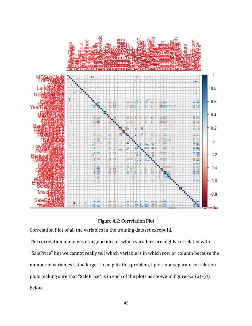
45

Figure 4.2: Correlation Plot

Correlation Plot of all the variables in the training dataset except Id.

The correlation plot gives us a good idea of which variables are highly correlated with

“SalePrice” but we cannot really tell which variable is in which row or column because the

number of variables is too large. To help fix this problem, I plot four separate correlation

plots making sure that “SalePrice” is in each of the plots as shown in figure 4.2 (a)-(d)

below.

46

Figure 4.3 (a)Correlation plot of the first 21 variables in the training data set with

“SalePrice”.

The plot has been modified to show correlations unlike in Figure 4.1 where the

correlations were displayed as colored squares.

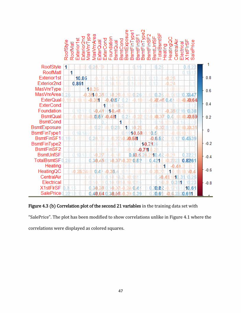
47

Figure 4.3 (b) Correlation plot of the second 21 variables in the training data set with

“SalePrice”. The plot has been modified to show correlations unlike in Figure 4.1 where the

correlations were displayed as colored squares.

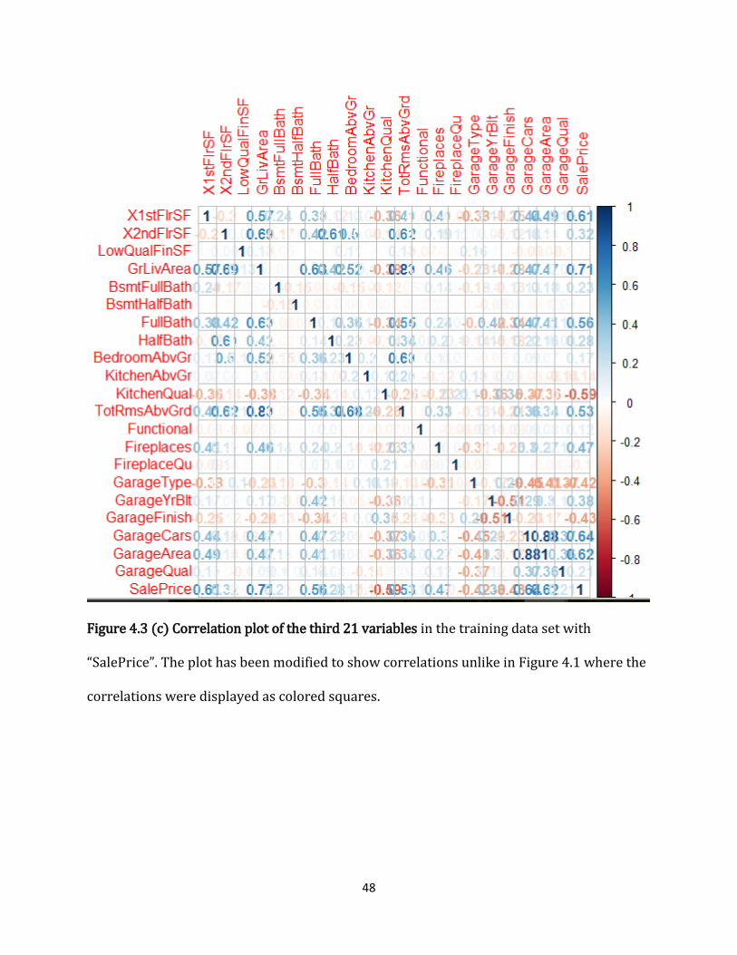
48

Figure 4.3 (c) Correlation plot of the third 21 variables in the training data set with

“SalePrice”. The plot has been modified to show correlations unlike in Figure 4.1 where the

correlations were displayed as colored squares.

49

Figure 4.3 (d) Correlation plot of the last 21 variables in the training data set with

“SalePrice”. The plot has been modified to show correlations unlike in Figure 4.1 where the

correlations were displayed as colored squares.

4.3.2 How to use “glmulti” to select variables to include in a model.

The results running the random forest algorithm above gives us a clue about which

variables are most important in determining the SalePrice of a house on individual bases.

50

For example, using the 𝐼𝑛𝑐𝑁𝑜𝑑𝑒𝑃𝑢𝑟𝑖𝑡𝑦 importance as criteria, we found that OverallQual is

the most important predictor. This means that if we had to build a model with only one

predictor, the one predictor should be OverallQual. However, we are interested in building

a model with more than one variable. To select the model with more than one variable, we

would feed the most important variables gotten from the random forest algorithm into the

“glmulti” function and run it. The results are the ‘best’ models with their support (by

default, the support is the Akaike Information Criteria (AIC), the relative quality of the

model judged by log likelihood) as well as the plot of their IC profile. The IC profile plot

shows how the IC changes from model (the one with the highest IC) the best to the worse

model (the one with the lowest IC). Below is the code for generating the best model, the

best model generated and the IC profile plot.

model.glmulti <- glmulti(SalePrice ~ Neighborhood + OverallQual +

YearBuilt + YearRemodAdd + MasVnrArea + Foundation + ExterQual +

Foundation + BsmtQual + BsmtFinSF1 + TotalBsmtSF + HeatingQC +

FullBath + CentralAir + KitchenQual + Fireplaces + GarageType +

GarageYrBlt + GarageCars + HouseSpace + BathRooms, data = train,

chunk=1, chunks=10, level = 1, minsize = 6, maxsize = 19, method =

"g", fitfunction = lm, confsetsize=90, crit = aicc)

best.model.glmulti <- lm(SalePrice ~ Neighborhood + ExterQual +

BsmtQual + CentralAir + KitchenQual + GarageType + OverallQual +

YearRemodAdd + BsmtFinSF1 + TotalBsmtSF + Fireplaces + GarageCars +

HouseSpace + BathRooms, train)

51

Figure 4.2: IC profile of best model using “glmulti”.

We see that the best model consists of those variables with high importance on the variable

importance plot which we had from random forest.

4.3.3 How to use Random Forest to select variables to include in a model.

This approach uses random forest to select the variables that are most related to

“SalePrice”. The variables are ranked by their ‘importance’ and a plot of the variables and

their importance can easily be gotten. This approach is especially helpful because it can

rank categorical and numeric variables alike. To use random forest to choose the most

related variables to “SalePrice”, we can run the following code.

install.packages(“randomForest”)

library(randomForest)

rf<-randomForest(SalePrice~.,data=train, importance=TRUE)

varImpPlot(rf)

importance(rf)

52

Figure 4.1: Variable Importance Plot Using Random Forest

Using Random Forests to Select the most important variables in building a model to predict

“SalePrice”.

The graph displays the variables in order of “importance” in a model used in predicting

“SalePrice”. The importance of each variable is given by the value on the horizontal axis

corresponding to the red circle on the line along the same horizon as the variable. Both

charts serve the same function only that one uses mean square error of prediction as the

criterion for choosing the variables while the other uses the loss function. It is still a matter

of debate which one to use in building a model- %𝐼𝑛𝑐𝑀𝑆𝐸 or 𝐼𝑛𝑐𝑁𝑜𝑑𝑒𝑃𝑢𝑟𝑖𝑡𝑦. Because of

this ambiguity, I choose to use the correlation plot of the variables to choose which

variables to include in my model.

53

4.4 Building and Discussing Model1

To build the first model, I set the minimum acceptable correlation coefficient to 0.35. This

means that any variable whose correlation with “SalePrice” is at least 0.35 can potentially

be included in the model. Looking back at the correlation plots in Figure 4.2 (a)-(d), we see

that following this criterion, the following variables are potential candidates for the model.

“OverallQual”, “YearBuilt”, “YearRemodAdd”, “ExterQual”, “BsmtQual”, “BsmtFinSF1”,

“TotBsmtSf”, “HeatingQC”, “1stFlrSF”, “GrLivArea”, “FullBath”, “TotRmsAbvGrg”,

“MasVnrArea”, “KitchenQual”, “Fireplaces”, “GarageType”, “GarageYrBlt”, “GarageFinish”,

“GarageCars”, “GarageArea”, “HouseSpace”, “BathRooms”. Below is the correlation plot for

these variables.

54

Figure 4.4 Correlation plot variables that are highly correlated with SalePrice

Correlation plot of all the variables that are highly correlated with “SalePrice”

Suppose we decide to fit a linear model called “model1” with all these variables, then we

will use the following line of code.

55

model1<- lm(SalePrice ~ Neighborhood + OverallQual + YearBuilt +

YearRemodAdd + MasVnrArea + Foundation + ExterQual + Foundation +

BsmtQual + BsmtFinSF1 + TotalBsmtSF + HeatingQC + FullBath +

CentralAir + KitchenQual + Fireplaces + GarageType + GarageYrBlt +

GarageCars + HouseSpace + BathRooms, data = train)

From the plot, we see that HouseSpace and GrdLivArea (quality living area on the first and

second floors) are perfectly correlated. There is also a high positive correlation between

HouseSpace and TotRoomsAbvGrd. For this reason, we exclude GrdLivArea and

TotRoomsAbvGrd from the first model. Since GarageCars and GarageArea are highly

correlated, we exclude GarageArea from, the model. Similarly, we exclude 1stFlrSF because

it is highly correlated with TotalBsmtSF. Besides, 1stFlrSF is included in the calculation of

HouseSpace. Though Neighborhood is not highly correlated with SalePrice, we include it in

the model. It is important to note that the reason why Neighborhood is not highly

correlated with SalePrice is because Neighborhood is a categorical variable with many

levels and suffers from the effect discussed earlier in section 2.5.3. For similar reasons, we

add CentralAir. And a summary of the model gives;

Residuals: Min 1Q Median 3Q Max -416260 -13469 496 12943 226513 Coefficients: Estimate Std. Error t value Pr(>|t|) (Intercept) -2.763e+05 2.025e+05 -1.364 0.172784 NeighborhoodBlueste -2.120e+04 2.391e+04 -0.887 0.375448 NeighborhoodBrDale -1.812e+04 1.209e+04 -1.499 0.134173 NeighborhoodBrkSide 8.438e+03 1.007e+04 0.838 0.402100 NeighborhoodClearCr 2.439e+04 1.031e+04 2.366 0.018120 * NeighborhoodCollgCr 1.714e+04 8.219e+03 2.085 0.037210 * NeighborhoodCrawfor 2.951e+04 9.889e+03 2.985 0.002889 ** NeighborhoodEdwards -8.183e+03 9.223e+03 -0.887 0.375109 NeighborhoodGilbert 9.357e+03 8.736e+03 1.071 0.284321 NeighborhoodIDOTRR -3.426e+03 1.072e+04 -0.320 0.749359 NeighborhoodMeadowV -1.515e+04 1.160e+04 -1.306 0.191720 NeighborhoodMitchel -1.738e+03 9.435e+03 -0.184 0.853838

56

NeighborhoodNAmes 1.626e+03 8.929e+03 0.182 0.855532 NeighborhoodNoRidge 6.968e+04 9.655e+03 7.217 8.68e-13 *** NeighborhoodNPkVill -1.583e+04 1.361e+04 -1.163 0.245002 NeighborhoodNridgHt 3.727e+04 8.856e+03 4.209 2.73e-05 *** NeighborhoodNWAmes -4.046e+02 9.205e+03 -0.044 0.964947 NeighborhoodOldTown -8.598e+03 9.760e+03 -0.881 0.378468 NeighborhoodSawyer 1.960e+03 9.369e+03 0.209 0.834297 NeighborhoodSawyerW 9.340e+03 8.974e+03 1.041 0.298134 NeighborhoodSomerst 2.245e+04 8.496e+03 2.643 0.008311 ** NeighborhoodStoneBr 5.735e+04 1.017e+04 5.639 2.06e-08 *** NeighborhoodSWISU -4.135e+02 1.134e+04 -0.036 0.970924 NeighborhoodTimber 2.038e+04 9.433e+03 2.160 0.030944 * NeighborhoodVeenker 3.688e+04 1.249e+04 2.952 0.003206 ** OverallQual 1.029e+04 1.201e+03 8.564 < 2e-16 *** YearBuilt -4.842e+01 8.314e+01 -0.582 0.560389 YearRemodAdd 1.994e+02 6.307e+01 3.161 0.001604 ** MasVnrArea 3.905e+00 5.839e+00 0.669 0.503733 FoundationCBlock 7.691e+03 3.930e+03 1.957 0.050548 . FoundationPConc 3.151e+03 4.363e+03 0.722 0.470241 FoundationSlab 8.414e+02 1.171e+04 0.072 0.942723 FoundationStone 7.495e+03 1.344e+04 0.558 0.577159 FoundationWood -4.407e+03 1.920e+04 -0.229 0.818522 ExterQualFa -1.904e+04 1.177e+04 -1.617 0.106015 ExterQualGd -2.123e+04 6.016e+03 -3.529 0.000430 *** ExterQualTA -2.131e+04 6.694e+03 -3.183 0.001490 ** BsmtQualFa -3.468e+04 7.784e+03 -4.455 9.06e-06 *** BsmtQualGd -3.213e+04 4.185e+03 -7.677 3.05e-14 *** BsmtQualNoBasement -2.629e+04 1.088e+04 -2.417 0.015782 * BsmtQualTA -3.114e+04 5.164e+03 -6.029 2.10e-09 *** BsmtFinSF1 1.003e+01 2.615e+00 3.836 0.000131 *** TotalBsmtSF 1.208e+01 3.330e+00 3.628 0.000296 *** HeatingQCFa -3.294e+03 5.344e+03 -0.616 0.537738 HeatingQCGd -4.126e+03 2.649e+03 -1.557 0.119640 HeatingQCPo -1.169e+04 3.227e+04 -0.362 0.717303 HeatingQCTA -4.406e+03 2.540e+03 -1.734 0.083050 . FullBath 1.907e+03 2.533e+03 0.753 0.451760 CentralAirY 8.992e+03 4.271e+03 2.105 0.035463 * KitchenQualFa -3.270e+04 7.660e+03 -4.269 2.09e-05 *** KitchenQualGd -2.745e+04 4.434e+03 -6.192 7.79e-10 *** KitchenQualTA -3.192e+04 4.983e+03 -6.405 2.04e-10 *** Fireplaces 6.319e+03 1.664e+03 3.798 0.000152 *** GarageTypeAttchd 4.019e+04 1.353e+04 2.970 0.003026 ** GarageTypeBasment 3.840e+04 1.544e+04 2.488 0.012974 * GarageTypeBuiltIn 4.436e+04 1.409e+04 3.150 0.001670 ** GarageTypeCarPort 1.897e+04 1.734e+04 1.094 0.273982 GarageTypeDetchd 3.513e+04 1.351e+04 2.601 0.009394 ** GarageTypeNoGarage 5.520e+04 1.540e+04 3.585 0.000349 *** GarageYrBlt -8.956e+01 7.055e+01 -1.270 0.204463 GarageCars 1.577e+04 2.056e+03 7.673 3.13e-14 *** HouseSpace 3.557e+01 3.200e+00 11.115 < 2e-16 *** BathRooms 4.473e+03 1.630e+03 2.745 0.006131 ** --- Signif. codes: 0 ‘***’ 0.001 ‘**’ 0.01 ‘*’ 0.05 ‘.’ 0.1 ‘ ’ 1 Residual standard error: 31420 on 1397 degrees of freedom Multiple R-squared: 0.8502, Adjusted R-squared: 0.8435 F-statistic: 127.9 on 62 and 1397 DF, p-value: < 2.2e-16

57

Judging by the Signif. Codes, we see that the most significant variables in model1 are;

“OverallQual, “YearRemodAdd”, “ExterQual”, “BsmtQual”, “BsmtFinSF1”, “KitchenQual”,

“Neighborhood”, “TotalBsmtSF”, “Fireplaces”, “GarageFinish”, “GarageCars”, “HouseSpace”.

Of course, we do not expect all the variables in the model to be significant because the

response variables are not really independent variables in the true sense of independence.

For example, “GarageCars” which is the number of cars that can fit in the garage is

supposed to be highly correlated with “GarageArea” because the number of cars that can fit

in a garage is a function of the area of the garage. The model produces an R-squared value

of 0.8502 and an adjusted R-squared value of 0.8435. This is not too bad but the standard

error of the residuals is too high. We can also see that the minimum and maximum

residuals are very large in value (respectively -416260 and 226513). The F-statistic of this

model is not as large as one should expect for a model with over 20 variables. It is but

normal to expect these extremes because the model includes a lot of variables with

insignificant coefficients. Further diagnosis of the model can be obtained by plotting the

model results. A plot of the model results can be obtained by the following line of code;

Plot(model1)

58

Figure 4.5: Residual analysis plots of the results of model1.

From the scale-location plot, we see that there is a trend in the residuals (the residuals

follow a quadratic trend which is difficult to see on the residuals vs fitted plot partly

because some points have very large residuals). This means that the model suffers from

heteroskedasticity. We can run a bptest on the model to be sure that our observation is

correct. We must do well to recall that the “bptest” uses null and alternative hypotheses;

𝐻0: 𝑇ℎ𝑒 𝑠𝑞𝑢𝑎𝑟𝑒𝑑 𝑟𝑒𝑠𝑖𝑑𝑢𝑎𝑙𝑠 𝑎𝑟𝑒 𝑛𝑜𝑡 𝑟𝑒𝑙𝑎𝑡𝑒𝑑 𝑡𝑜 𝑡ℎ𝑒 𝑟𝑒𝑠𝑝𝑜𝑛𝑠𝑒 𝑣𝑎𝑟𝑖𝑎𝑏𝑙𝑒𝑠.(NULL)

𝐻1: 𝑇ℎ𝑒 𝑠𝑞𝑢𝑎𝑟𝑒𝑑 𝑟𝑒𝑠𝑖𝑑𝑢𝑎𝑙𝑠 𝑎𝑟𝑒 𝑟𝑒𝑙𝑎𝑡𝑒𝑑 𝑡𝑜 𝑡ℎ𝑒 𝑟𝑒𝑠𝑝𝑜𝑛𝑠𝑒 𝑣𝑎𝑟𝑖𝑏𝑙𝑒𝑠. (ALTERNATIVE)

bptest(model1)

studentized Breusch-Pagan test

data: model1BP = 567.15, df = 62, p-value < 2.2e-16

59

We see that the p-value is almost zero (𝑝 − 𝑣𝑎𝑙𝑢𝑒 < 2.2 ∗ 10−16). This means that the

probability of having a result in which the squared residuals are not related to the response

variables using model1 is almost zero. Thus, we must conclude that the squared residuals

of results of model1 are related to the response variables in the model. We should

therefore reject the null hypothesis and conclude that model1 suffers from

heteroskedasticity. To see how the variance of the errors changes, that is whether it is

increasing or decreasing along segments of the data set from left to right, we can run a

“gqtest” on model1. The results of a “gqtest” on model1 are right below.

𝐻0: 𝑇ℎ𝑒 𝑣𝑎𝑟𝑖𝑎𝑡𝑖𝑜𝑛 𝑖𝑛 𝑚𝑜𝑑𝑒𝑙1 𝑟𝑒𝑠𝑖𝑑𝑢𝑎𝑙𝑠 𝑖𝑠 𝑐𝑜𝑛𝑠𝑡𝑎𝑛𝑡 𝑓𝑟𝑜𝑚 𝑠𝑒𝑔𝑚𝑒𝑛𝑡 1 𝑡𝑜 2.

𝐻1: 𝑇ℎ𝑒 𝑣𝑎𝑟𝑖𝑎𝑡𝑖𝑜𝑛 𝑖𝑛 𝑚𝑜𝑑𝑒𝑙1 𝑟𝑒𝑠𝑖𝑑𝑢𝑎𝑙𝑠 𝑖𝑛𝑐𝑟𝑒𝑎𝑠𝑒𝑠 𝑓𝑟𝑜𝑚 𝑠𝑒𝑔𝑚𝑒𝑛𝑡 1 𝑡𝑜 2.

gqtest(model1)

Goldfeld-Quandt testdata: model1

GQ = 1.0946, df1 = 667, df2 = 667, p-value = 0.1216

alternative hypothesis: variance increases from segment 1 to 2

The p-value for this test is 0.1216 which is greater than the level of significance 𝛼 = .05.

This means there is not enough reason to conclude that the variance increases from

segment 1 (left) to segment 2 (right). Therefore, we must not reject the null hypothesis

meaning there is no heteroskedasticity. The conclusion from one test contradicts the

conclusion from the other. This might mean there is undetectable (unconditional)

heteroskedasticity. Notice that the trend in the residuals is such that higher sales prices

produce higher residual. This might be conditional heteroskedasticity caused by

misspecification of the model or unconditional heteroskedasticity relating to the fact that

those who buy large houses are usually the richer folks and corporations which are not too

60

restricted by money and have a higher variability in spending. Notice that all four graphs

indicate the presence of outliers. A look at the normal Q-Q plot shows that most of the

points lie on the theoretical line though a few of them are quite off the line. These are the

outliers. They show themselves on all four plots. Apart from the outliers, most of the points

in the residuals vs leverage plot have small cook distance. Since scale locations greater than

2.5 are generally not good, we may need to remove the outliers and the insignificant

variables, build another model and evaluate it. Let us call this new model model2.

4.5 Building and Discussing Model2

It is possible that we might have missed certain trends of the variables, to fix this, we will

need to plot the graphs of the relationship between the variables and “SalePrice”. To get

these correlations, we must first get the indices (row numbers corresponding to variable

names) of these variables. The following line of code does this for us.

which(names(train)=="OverallQual")

which(names(train)=="YearBuilt")

For simplicity, I have included only the line of code for “OverallQual” and “YearBuilt” but

similar one could do the same for every other variable. We use R to get the correlation plot.

The resulting correlation plot is below. It is important to keep in mind that we are using the

correlation plot to determine which numerical variables to include in our model. As for

categorical variables, our judgement will come from the random forest plot and the models

that glmulti would generate for us.

61

Figure 4.6: Correlation Plot for the variables in model1

I order to fully utilize this correlation plot, we will need to choose a criterion for judging

whether any variable predicts the other. Setting the correlation level to 65% (𝑖𝑒 |𝑟| ≥

0.65), and taking the more correlated variable with SalePrice, we see that the following

variables would be excluded- “YearBuilt” and “GarageYrBlt”. Thus, our new model, model2

shall include only the following variables. “Neighborhood”, “OverallQual”,

“YearRemodAdd”, “MasVnrArea”, “ExterQual”, “Foundation”, “BsmtQual”, “TotBsmtSF”,

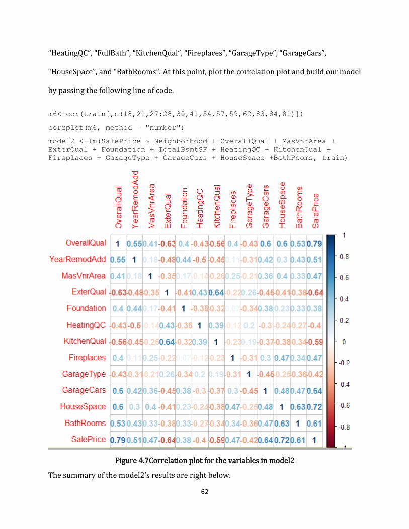
62

“HeatingQC”, “FullBath”, “KitchenQual”, “Fireplaces”, “GarageType”, “GarageCars”,

“HouseSpace”, and “BathRooms”. At this point, plot the correlation plot and build our model

by passing the following line of code.

m6<-cor(train[,c(18,21,27:28,30,41,54,57,59,62,83,84,81)])

corrplot(m6, method = "number")

model2 <-lm(SalePrice ~ Neighborhood + OverallQual + MasVnrArea +

ExterQual + Foundation + TotalBsmtSF + HeatingQC + KitchenQual +

Fireplaces + GarageType + GarageCars + HouseSpace +BathRooms, train)

Figure 4.7Correlation plot for the variables in model2

The summary of the model2’s results are right below.

63

Summary(model2)

Residuals: Min 1Q Median 3Q Max -121108 -13545 186 12979 201312 Coefficients: Estimate Std. Error t value Pr(>|t|) (Intercept) -5.097e+05 1.054e+05 -4.837 1.46e-06 *** NeighborhoodBlueste -7.356e+03 2.038e+04 -0.361 0.718226 OverallQual 1.038e+04 1.007e+03 10.312 < 2e-16 *** YearRemodAdd 2.455e+02 5.243e+01 4.682 3.12e-06 *** MasVnrArea 1.315e+01 4.997e+00 2.632 0.008571 ** ExterQualFa -3.601e+04 9.968e+03 -3.613 0.000314 *** FoundationCBlock 8.687e+03 3.129e+03 2.776 0.005571 ** TotalBsmtSF 3.357e+01 2.540e+00 13.217 < 2e-16 *** HeatingQCFa -3.189e+03 4.388e+03 -0.727 0.467511 KitchenQualFa -3.602e+04 6.473e+03 -5.565 3.14e-08 *** Fireplaces 6.052e+03 1.392e+03 4.347 1.48e-05 *** GarageTypeAttchd 4.590e+04 1.146e+04 4.007 6.48e-05 *** GarageCars 1.236e+04 1.674e+03 7.388 2.55e-13 *** HouseSpace 3.944e+01 2.432e+00 16.213 < 2e-16 *** BathRooms 6.596e+03 1.167e+03 5.652 1.92e-08 *** --- Signif. codes: 0 ‘***’ 0.001 ‘**’ 0.01 ‘*’ 0.05 ‘.’ 0.1 ‘ ’ 1 Residual standard error: 26820 on 1401 degrees of freedom Multiple R-squared: 0.8796, Adjusted R-squared: 0.875 F-statistic: 193.1 on 53 and 1401 DF, p-value: < 2.2e-16 #Note: I have only shown the first level, for every categorical variable.

Notice that we have succeeded in removing 8 variables from the first model. Yet, the R-

squared and adjusted R-Squared have significantly increased (more than 3 percentage

points). Further, only three of the 14 variables in the model display insignificant

coefficients. The F statistic has also increased from 127.9 to 193.1 and the residual

standard error has dropped from 31420 to 26820. The range of the residuals has also

greatly reduced (from 642773 to 322420). Let us look at the plot of the model. The

following lines of code will help get the plots for us.

Plot(model2)

64

Figure 4.8: Plot summary of model2

From the Residuals vs Fitted plot, we see that the residuals not only increase in spread

from left to right, but also seem to follow a C-like quadratic trend. This means that the

model still suffers from heteroskedasticity. Running a Breusch-Pagan and a Goldfeld-

Quandt tests on model2 yields the following results.

bptest(model2)

studentized Breusch-Pagan test

data: model2

BP = 234.61, df = 53, p-value < 2.2e-16

gqtest(model2)

Goldfeld-Quandt test

data: model2

GQ = 0.83435, df1 = 674, df2 = 673, p-value = 0.9906

alternative hypothesis: variance increases from segment 1 to 2

65

Notice that the two test again result in conflicting conclusions. While the studentized

Breusch-Pagan says, there is heteroskedasticity, the Goldfeld-Quandt says there is no

heteroskedasticity. We can now be sure that the trend in the errors that we are seeing is

likely due to increasing spreads in the variables from left to right and thus cannot be fixed.

Though we have taken out the initial set of outliers that model1 displayed, other outliers

have resurfaced. This will always be the case till a perfect model is fitted. But there is no

such thing as a perfect model meaning we will always have outliers showing up. Though

the Q-Q plot has improved (we no longer have any standardized residuals greater than 10

in absolute value), the large curve in its right end suggests that we have a problem in

predicting the prices for houses that cost more money. This supports the fact that the

errors in the model are increasing from left to right. We can also see that the cook distances

have reduced (we no longer have points with cook distances greater than 0.5) and the F-

statistic has increased by over 60 points. Overall, the model has improved, but more work

needs to be done to make it even better.

4.6 Building and Discussing Model3

Let us return to the model suggested by glmulti algorithm that we ran earlier. Recall that

the algorithm had suggested that the best linear model would be the following.

model.best.glmulti<-lm(SalePrice ~ Neighborhood + ExterQual + BsmtQual

+ CentralAir + KitchenQual + GarageType + OverallQual + YearRemodAdd +

BsmtFinSF1 + TotalBsmtSF + Fireplaces + GarageCars + HouseSpace + Bath

Rooms, train)

Going back to model2 above, we see that the two models have many variables in common.

The only conflicting variables in these models are CentralAir, BsmtFinSF1, Foundation,

66

MasVnrArea, and HeatingQC. The summary of model2 already revealed to us that

HeatingQC and Foundation were not significant variables. Running a summary of

model.best.glmulti also reveals that Bathrooms is not significant. Thus, we can exclude

BathRooms, HeatingQC and Foundation from our next model.

To deal with the reoccurring problem of heteroskedasticity, we will plot some scatter plots

to see if we are missing some trend in the data.

par(mfrow=c(2,2))

plot(SalePrice ~ OverallQual, col='blue', train)

abline(lm(SalePrice ~ OverallQual, col='red', train))

plot(SalePrice ~ MasVnrArea, col='blue', train)

plot(SalePrice ~ ExterQual, col='blue', train)

plot(SalePrice ~ CentralAir, col='blue', train)

plot(SalePrice ~ HeatingQC, col='blue', train)

plot(SalePrice ~ KitchenQual, col='blue', train)

plot(SalePrice ~ Fireplaces, col='blue', train)

plot(SalePrice ~ GarageFinish, col='blue', train)

plot(SalePrice ~ GarageCars, col='blue', train)

plot(SalePrice ~ HouseSpace, col='blue', train)

abline(lm(SalePrice ~ HouseSpace, col='red', train))

plot(SalePrice ~ YearRemodAdd, col='blue', train)

plot(SalePrice ~ FullBath, col='blue', train)

Below are the plots. From the plots, we see that “HouseSpace” and “OverallQual” seem to

display quadratic trends. We will include these trends in our third model and call it model3.

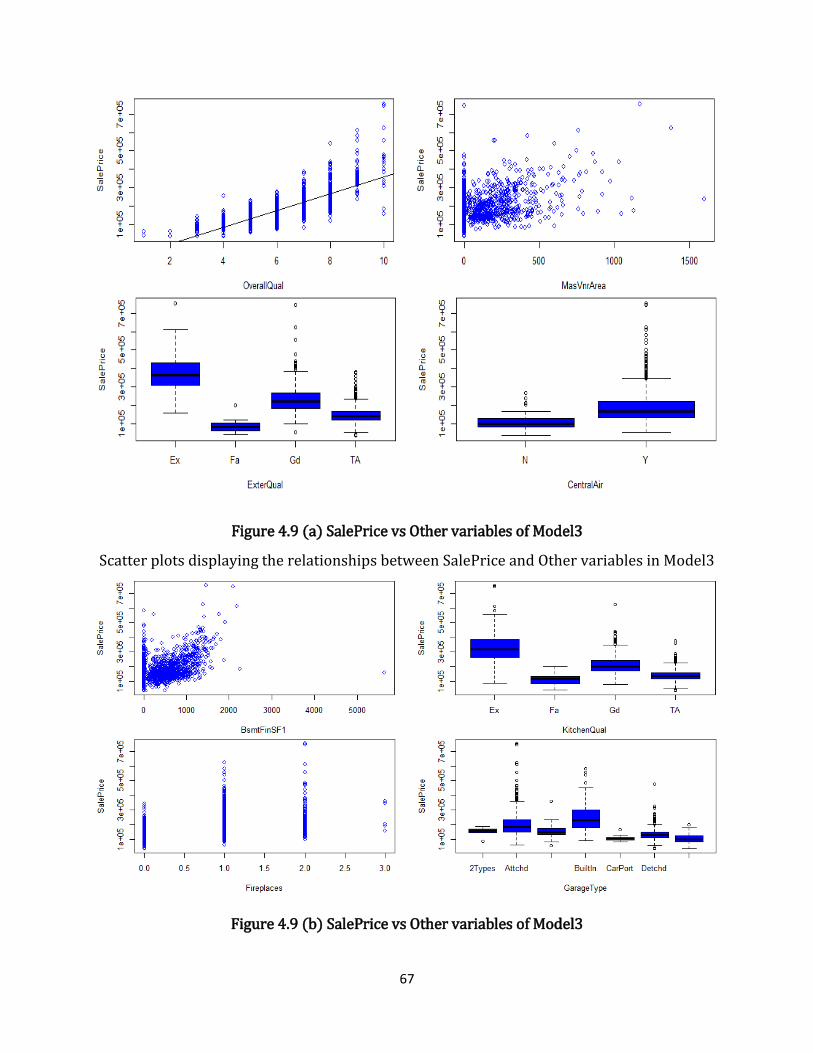
67

Figure 4.9 (a) SalePrice vs Other variables of Model3

Scatter plots displaying the relationships between SalePrice and Other variables in Model3

Figure 4.9 (b) SalePrice vs Other variables of Model3

68

Scatter plots displaying the relationships between SalePrice and Other variables in Model3

Figure4.9 (c) SalePrice vs. HouseSpace and Neighborhood.

Scatter plots displaying the relationships between SalePrice and Other variables in Model3

The shape of the scatter plot of SalePrice vs OverallQual seems more like a parabola than a

line. This means OverallQual would be best represented by a quadratic than a line. Since we

did not include quadratic terms for OverallQual in model2, it was likely an underfit. The

plots that look like series of box plots are the scatter plots for categorical variables. For

69

those plots, each box plot is drawn for a level of the variable. For instance, CentralAir has

two categories, Y and N. (A box plot consists of the minimum value, first quartile, median,

third quartile and the maximum value. Any outliers are also indicated on the box plot above

the maximum value or below the minimum value). Thus, we have two box plots in the

scatter plot of SalePrice vs. CentralAir. Below is the summary and plot of model3.

Summary(model3)

plot(model3)

Residuals: Min 1Q Median 3Q Max -129964 -13068 948 12364 154396 Coefficients: Estimate Std. Error t value Pr(>|t|) (Intercept) -4.604e+05 9.654e+04 -4.768 2.05e-06 *** NeighborhoodBlueste 6.247e+02 1.919e+04 0.033 0.974041 NeighborhoodBrDale -7.277e+03 9.424e+03 -0.772 0.440113 NeighborhoodBrkSide 1.038e+04 7.501e+03 1.383 0.166791 NeighborhoodClearCr 3.245e+04 8.122e+03 3.995 6.81e-05 *** NeighborhoodCollgCr 1.928e+04 6.600e+03 2.922 0.003537 ** NeighborhoodCrawfor 3.228e+04 7.459e+03 4.328 1.61e-05 *** NeighborhoodEdwards 7.931e+03 7.178e+03 1.105 0.269381 NeighborhoodGilbert 1.929e+04 6.970e+03 2.767 0.005724 ** NeighborhoodIDOTRR 2.127e+02 8.026e+03 0.027 0.978860 NeighborhoodMeadowV -9.122e+03 9.249e+03 -0.986 0.324186 NeighborhoodMitchel 1.123e+04 7.475e+03 1.503 0.133129 NeighborhoodNAmes 9.665e+03 6.846e+03 1.412 0.158229 NeighborhoodNoRidge 3.806e+04 7.819e+03 4.867 1.26e-06 *** NeighborhoodNPkVill 2.844e+03 1.074e+04 0.265 0.791202 NeighborhoodNridgHt 3.376e+04 7.149e+03 4.722 2.57e-06 *** NeighborhoodNWAmes 9.234e+03 7.191e+03 1.284 0.199299 NeighborhoodOldTown -8.014e+03 7.097e+03 -1.129 0.259013 NeighborhoodSawyer 1.010e+04 7.272e+03 1.389 0.165066 NeighborhoodSawyerW 1.547e+04 7.153e+03 2.163 0.030732 * NeighborhoodSomerst 2.482e+04 6.839e+03 3.629 0.000295 *** NeighborhoodStoneBr 5.180e+04 8.168e+03 6.342 3.04e-10 *** NeighborhoodSWISU 3.593e+03 8.537e+03 0.421 0.673911 NeighborhoodTimber 2.713e+04 7.520e+03 3.608 0.000319 *** NeighborhoodVeenker 4.668e+04 9.907e+03 4.712 2.69e-06 *** I(OverallQual) -2.499e+04 4.052e+03 -6.168 9.01e-10 *** I(OverallQual^2) 3.061e+03 3.357e+02 9.120 < 2e-16 *** YearRemodAdd 3.119e+02 4.810e+01 6.485 1.22e-10 *** MasVnrArea 1.177e+01 4.716e+00 2.495 0.012709 * ExterQualFa -3.529e+04 9.265e+03 -3.809 0.000146 *** ExterQualGd -2.202e+04 4.969e+03 -4.432 1.00e-05 *** ExterQualTA -2.193e+04 5.533e+03 -3.964 7.75e-05 *** TotalBsmtSF 3.041e+01 2.138e+00 14.224 < 2e-16 *** KitchenQualFa -2.908e+04 6.114e+03 -4.757 2.17e-06 ***

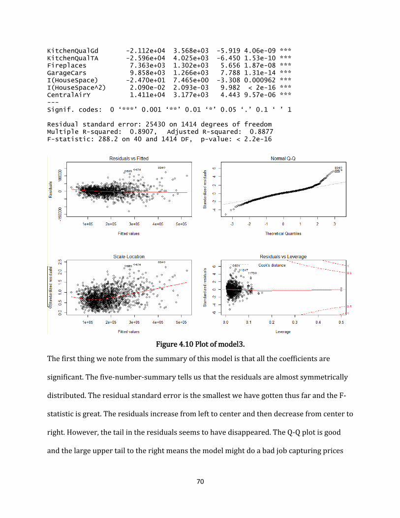
70

KitchenQualGd -2.112e+04 3.568e+03 -5.919 4.06e-09 *** KitchenQualTA -2.596e+04 4.025e+03 -6.450 1.53e-10 *** Fireplaces 7.363e+03 1.302e+03 5.656 1.87e-08 *** GarageCars 9.858e+03 1.266e+03 7.788 1.31e-14 *** I(HouseSpace) -2.470e+01 7.465e+00 -3.308 0.000962 *** I(HouseSpace^2) 2.090e-02 2.093e-03 9.982 < 2e-16 *** CentralAirY 1.411e+04 3.177e+03 4.443 9.57e-06 *** --- Signif. codes: 0 ‘***’ 0.001 ‘**’ 0.01 ‘*’ 0.05 ‘.’ 0.1 ‘ ’ 1 Residual standard error: 25430 on 1414 degrees of freedom Multiple R-squared: 0.8907, Adjusted R-squared: 0.8877 F-statistic: 288.2 on 40 and 1414 DF, p-value: < 2.2e-16

Figure 4.10 Plot of model3.

The first thing we note from the summary of this model is that all the coefficients are

significant. The five-number-summary tells us that the residuals are almost symmetrically

distributed. The residual standard error is the smallest we have gotten thus far and the F-

statistic is great. The residuals increase from left to center and then decrease from center to

right. However, the tail in the residuals seems to have disappeared. The Q-Q plot is good

and the large upper tail to the right means the model might do a bad job capturing prices

71

for houses that are supposed to be high. Scale Locations are good and Cook’s distances are

short. Testing for heteroskedasticity for the model gives the following results.

bptest(model3) studentized Breusch-Pagan test data: model3 BP = 258.19, df = 40, p-value < 2.2e-16 gqtest(model3) Goldfeld-Quandt test data: model3 GQ = 0.81556, df1 = 687, df2 = 686, p-value = 0.9962 alternative hypothesis: variance increases from segment 1 to 2

The two tests still conflict. The Breusch – Pagan test says the model suffers from

heteroskedasticity while the Goldfeld - Quandt teat says it does not. This difference arises

because both tests are using different criteria for testing heteroskedasticity. But this

usually happens when a model suffers from unconditional heteroskedasticity. We can

therefore conclude that the model suffers from unconditional heteroskedasticity. The

following table shows a summary of all three models.

Table 1: Summary of all three models.

R-Squared Adj R-Squared Number of Parameters (F-Stat, DF1, DF2) Residual Standard Error

model1 0.8502 0.8435 63 (127.9,62,1397) 31420

model2 0.8796 0.875 54 (193.1,53,1401) 26820

model3 0.8907 0.8877 41 (288.2,40,1414) 25430

P-value, BP test P-value, GQ test Min Residual Max Residual Residual Range

model1 < 2.2e-16 0.1216 -416260 226513 642773

model2 < 2.2e-16 0.9906 -121108 201312 322420

model3 < 2.2e-16 0.9962 -129964 154396 284360

72

The table helps us see that the models are generally improving from the first to the third.

For example, the adjusted R-squared value increases from 0.8435 in model1 through

0.8750 in model2 and ends at 0.8877 for model three. This is especially remarkable given

that the number of parameters being estimated (and therefore the number of predictors)

have also decreased from 63 in model1 through 54 in model2 to 41 in the third model.

The p-value for the Breusch Pagan test is the one exception to the trend of improving

attributes of the model. This p-value is less than 2.2 ∗ 10−16 in all three models while its

brother Goldfeld Quandt test p-value increases from model1 to model3. The conflicting

conclusions that results from these two tests is proof of unconditional heteroskedasticity.

In the next chapter, we explore how to use our model.

73

CHAPTER 5

USING THE MODEL

As was pointed out in chapter 1, one of the goals of this thesis is build a model that can be

used to predict sales prices for houses. Having built our model, it remains to use this model

to predict sales prices on the testing data set. This can easily be done using software but

before doing so, one must make sure all the variables in the test data set are of the same

class and structure as those in the training data set that was used in building the model.

This means that one must go through the following process again

• Fill the missing values in the test data, for example

test$BsmtCond<-as.character(test$BsmtCond)

test$BsmtCond[is.na(test$BsmtCond)]<-"NoBasement"

test$BsmtCond<-as.factor(test$BsmtCond)

test$BsmtCond<-as.numeric(test$BsmtCond)

• Convert variables to the appropriate form that the built model can use,

test$BsmtHalfBath[is.na(test$BsmtHalfBath)]<-0

test$BsmtFullBath[is.na(test$BsmtFullBath)]<-0

test$BsmtUnfSF[is.na(test$BsmtUnfSF)]<-0

• Calculate all the new variables that were calculated for the training set,

test$HouseSpace<-as.numeric(test$X1stFlrSF+test$X2ndFlrSF+test$

TotalBsmtSF)

• Include the variable “SalePrice” that was in the training set but not in the test set.

test<-data.frame(SalePrice=rep("0", nrow(test)), test[,])

test$SalePrice<-as.numeric(test$SalePrice)

After all this must have been done, the following lines of code can be applied to predict the

“SalePrice” for the data in the test data set.

test$SalePrice<-predict(model3,test)#to predict the sale prices

summary(test$SalePrice)#view five number summary of these sale prices

results<-data.frame(Id=test$Id, SalePrice=test$SalePrice)

summary(results)

write.csv(results,"Mode3_results.csv")#Export these results as csv.

74

This completes the goal of forecasting house prices using the model we just built. However,

it would not make sense for an individual looking to predict the price of a house he wants

to buy or sell by casting the points into a data frame. In such a case, one would only get the

coefficients for the variables and insert them in a calculator to get the price. For instance,

suppose we wanted to predict the worth of a house having the following parameters;

Neighborhood = “Gilbert”,

“OverallQual” rating of 8,

“YearRemodAdd” = 2006,

“MasVnrArea” = 180,

“ExterQual” rated as “Gd”,

“TotalBsmtSF” = 1060,

“KitchenQual” rated as “Gd”,

“Fireplaces” = 2,

“GarageCars” = 2,

“HouseSpace” = 2000,

“CentralAir” = “Y”

There are several ways to put these values into the model for prediction. One would have

to copy the model coefficients (from the model summary or by passing coef(model3)) and

use these coefficients to calculate the predicted price. In the case of the above figures, we

would get;

MyPrice<- coef(model3)[1]+coef(model3)[9]+ coef(model3)[26]*8+ coef(mo

del3)[27]*8^2+coef(model3)[28]*2006+ coef(model3)[29]*180+coef(model3)

[31]+ coef(model3)[33]*1060+coef(model3)[35]+ coef(model3)[37]*2+coef(

75

model3)[38]*2+ coef(model3)[39]*2000+coef(model3)[40]*2000^2+ coef(mod

el3)[41]

MyPrice

254554.3.

This means a house with the above parameters should be worth about $250,000 by our

model. Anyone can then be able to change the parameters to suite their situation. This

completes the task of forecasting with the model we built.

It is important to note that the model that we have built is mostly mathematical. We have

used mathematical techniques to determine which variables have a high effect on the sale

price of a house and used those variables in determining the price of a house. This does not

in any way mean the other variables are not as important. We know the type of foundation

and the roof materials are very important price determinants but these did not prove to be

important in our case. Those variables which we did not include in our model, but which

influence the house prices are called lurking variables. Since our final model included 3

variables, we had at least 70 lurking variables.

76

CHAPTER 6

FINDINGS AND CONCLUSION

The main motivation for this thesis is related to the fact that many individuals and

businesses must make decisions about buying houses and business quarters but they are

often unable to make these decisions without the intervention of experts because a large

volume of information must be processed to determine the price of each property. This

thesis was aimed at helping people with little or no experience to understand just which

variables are important in determining the price of a house and how to use those variables

to determine the price of the given house. In the following table shows the importance of

each variables in determining the price of a house and the weight attributed to each

variable. An additional column called Variable Description has be included to help readers

understand the variables.

Variable Name Variable Description Importance %IncMSE

Importance IncNodePurity

HouseSpace Total area of 1st and 2nd floor plus basement 37.47 2.18E+12 OverallQual 1 to 10 rating of the overall quality of the house 24.91 1.86E+12 GrLivArea Total living area above basement 19.37 5.81E+11 X1stFlrSF Area of first floor 16.87 2.01E+11 YearBuilt Original year the house was built 16.26 3.64E+11 GarageCars Maximum garage capacity in number of cars 14.90 4.42E+11 GarageArea Total area of garage 14.72 2.78E+11 TotalBsmtSF Total area of the basement 13.55 1.43E+11 plotArea Total area of the plot 13.41 9.61E+10 GarageType The type of Garage (attached or detached from ho

use 13.21 5.53E+10

ExterQual Quality of Materials on the exterior of the house 13.17 5.02E+11 YearRemodAdd Year the house was remodeled (if applicable) 13.13 9.27E+10 Rooms Total number of rooms in the house 12.86 2.49E+11 MSZoning Economic activity associated with the location of t

he house 12.41 1.56E+10

OverallCond 1 to 10 rating of the overall condition of the house 12.08 3.31E+10 GarageYrBlt Year the garage was built 11.83 4.51E+10 BsmtFinSF1 Total finished area of basement (1st rating) 11.63 7.40E+10 LotArea Lot Area of the property 11.58 8.51E+10 MSSubClass Type of dwelling involved with the sale 11.54 1.94E+10

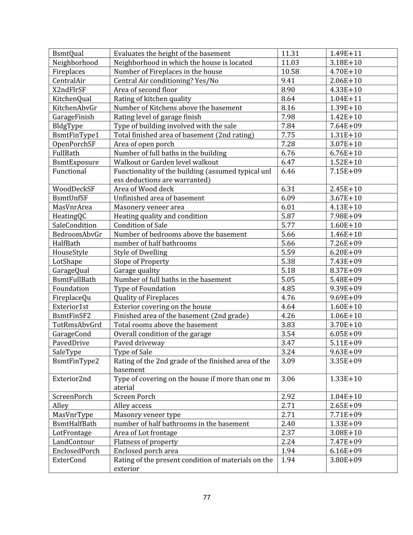
77

BsmtQual Evaluates the height of the basement 11.31 1.49E+11 Neighborhood Neighborhood in which the house is located 11.03 3.18E+10 Fireplaces Number of Fireplaces in the house 10.58 4.70E+10 CentralAir Central Air conditioning? Yes/No 9.41 2.06E+10 X2ndFlrSF Area of second floor 8.90 4.33E+10 KitchenQual Rating of kitchen quality 8.64 1.04E+11 KitchenAbvGr Number of Kitchens above the basement 8.16 1.39E+10 GarageFinish Rating level of garage finish 7.98 1.42E+10 BldgType Type of building involved with the sale 7.84 7.64E+09 BsmtFinType1 Total finished area of basement (2nd rating) 7.75 1.31E+10 OpenPorchSF Area of open porch 7.28 3.07E+10 FullBath Number of full baths in the building 6.76 6.76E+10 BsmtExposure Walkout or Garden level walkout 6.47 1.52E+10 Functional Functionality of the building (assumed typical unl

ess deductions are warranted) 6.46 7.15E+09

WoodDeckSF Area of Wood deck 6.31 2.45E+10 BsmtUnfSF Unfinished area of basement 6.09 3.67E+10 MasVnrArea Masonery veneer area 6.01 4.13E+10 HeatingQC Heating quality and condition 5.87 7.98E+09 SaleCondition Condition of Sale 5.77 1.60E+10 BedroomAbvGr Number of bedrooms above the basement 5.66 1.46E+10 HalfBath number of half bathrooms 5.66 7.26E+09 HouseStyle Style of Dwelling 5.59 6.20E+09 LotShape Slope of Property 5.38 7.43E+09 GarageQual Garage quality 5.18 8.37E+09 BsmtFullBath Number of full baths in the basement 5.05 5.48E+09 Foundation Type of Foundation 4.85 9.39E+09 FireplaceQu Quality of Fireplaces 4.76 9.69E+09 Exterior1st Exterior covering on the house 4.64 1.60E+10 BsmtFinSF2 Finished area of the basement (2nd grade) 4.26 1.06E+10 TotRmsAbvGrd Total rooms above the basement 3.83 3.70E+10 GarageCond Overall condition of the garage 3.54 6.05E+09 PavedDrive Paved driveway 3.47 5.11E+09 SaleType Type of Sale 3.24 9.63E+09 BsmtFinType2 Rating of the 2nd grade of the finished area of the

basement 3.09 3.35E+09

Exterior2nd Type of covering on the house if more than one material

3.06 1.33E+10

ScreenPorch Screen Porch 2.92 1.04E+10 Alley Alley access 2.71 2.65E+09 MasVnrType Masonry veneer type 2.71 7.71E+09 BsmtHalfBath number of half bathrooms in the basement 2.40 1.33E+09 LotFrontage Area of Lot frontage 2.37 3.08E+10 LandContour Flatness of property 2.24 7.47E+09 EnclosedPorch Enclosed porch area 1.94 6.16E+09 ExterCond Rating of the present condition of materials on the

exterior 1.94 3.80E+09

78

BsmtCond Rating of the present condition of materials on the basement

1.57 3.47E+09

Condition1 Proximity to various conditions 1.57 3.94E+09 PoolArea Area of Pool (if applicable) 1.36 1.48E+08 YrSold Year the house was sold 1.29 9.53E+09 Fence Type of Fence 1.27 3.55E+09 PoolQC Pool quality 1.18 3.15E+08 MoSold Moth the house was sold 0.93 1.93E+10 Id Id associated with the sale 0.92 2.62E+10 LandSlope Slope of Property 0.87 6.93E+09 RoofStyle Style of Roof 0.51 8.38E+09 Electrical Type of electrical system in the house 0.43 1.54E+09 Heating Type of Heating 0.29 1.07E+09 X3SsnPorch Three season porch area 0.17 1.36E+09 Utilities Type of utilities available 0.00 1.81E+06 LotConfig Lot Configuration -0.04 5.09E+09 MiscFeature Any miscellaneous features -0.29 5.67E+08 LowQualFinSF Area of low quality finished areas -0.31 1.46E+09 MiscVal $value of miscellaneous features -0.97 5.83E+08 Street Type of road access to property -1.08 2.76E+08 RoofMatl Type Roof Material -1.13 2.28E+09 Condition2 Proximity to various conditions if more than one i

s present -1.34 1.68E+08

Table 2: Ranking of variables by their importance.

Rankings of variables in decreasing order of importance in predicting SalePrice

From the table, we see that the most important variable in determining the price of a house

is “HouseSpace” which is the sum of the areas of the basement and the floors. Judging by

these rankings, we see that a fence is not as important as the neighborhood in determining

the price of a house. Other very important contributors to the sales price of the house that

are not very popular include the major economic activity associated with the location of the

house, the type of garage and the year it was built.

There are also some factors that are usually highly appraised but which do not contribute a

lot to the general value of the house. Two of these factors are the presence of a pool and a

fence. One of the reasons why our model might not have seen these factors as important is

79

that only few houses have them. For example, in the training set, only four houses had a

pool. This makes modelling difficult.

In this thesis, I have used the free programming language R to build my models and do my

analysis but other softwares such as MATLAB, and Python could also be used. I have also

built a linear model but one could also build a generalized linear model. Finally, compared

to the amount of large dataset out there, the dataset that I used is a small dataset. However,

the method and processes can still be applied to big data without much effort.

80

REFERENCES

References

Abu-Mostafa, Y. S., Magdon-Ismail, M., & Lin, H.-T. (2012). Learning from Data.

AMLbook.com.

Benoit, K. (2010, November 24). Ordinary Least Squares Regression. Retrieved from

http://www.kenbenoit.net/courses/quant1/Quant1_Week8_OLS.pdf

Breiman, L., & Cutler, A. (2004, 06 15). Random Forests. Retrieved 04 19, 2017, from

http://www.stat.berkeley.edu/~breiman/RandomForests/cc_home.htm

Calcagno, V. (2013, 04 10). Package 'glmulti'. Retrieved from https://cran.r-

project.org/web/packages/glmulti/glmulti.pdf

Calcagno, V., & Claire, M. (2010, 05). glmulti: An R Package for Easy Automated Model

Selection with (Generalized) Linear Models. Journal of Statistical Software, 34(12),

1.

Carr, D. H., Lawson, J. A., & Schultz, J. C. (2010, 02 21). Influences of Real Estate. In D. H.

Carr, J. A. Lawson, & J. C. Schultz, Mastering Real Estate Appraisal. Retrieved from

http://www.ctrealtor.com/unprotected/Ch01.pdf

Dan Campbell, S. C. (2008). Introduction to Regression and Data Analysis. Introduction to

Regression and. Data Analysis with. Dan Campbell and Sherlock Campbel (p. 6). Yale

Statlap. Retrieved 02 14, 2017, from

http://statlab.stat.yale.edu/workshops/IntroRegression/StatLab-

IntroRegressionFa08.pdf

81

Edwards, A. W. (1992). Likelihood Expanded Edition. Baltimore: John Hopkins university

Press. Retrieved from Wikipedia.

Fawumi, K. (2015, 12 05). DESIGN OF AN INTERACTIVE AND WEB-BASED SOFTWARE FOR

THE MANAGEMENT, ANALYSIS AND TRANSFORMATION OF TIME SERIES.

Retrieved from Sebis Public Website:

https://wwwmatthes.in.tum.de/pages/2n64q4x31bo/Master-s-Thesis-Kehinde-

Fawumi

Flinn, C. (2004, 10 01). Discussion of the Gauss-Markov Theorem. Retrieved from

econ.nyu.edu: http://www.econ.nyu.edu/user/flinnc/courses/0266-06/gauss-

markov-theorem.pdf

Frost, J. (2015, 09 03). The Danger of Overfitting a Regression Model. Retrieved from

Minintab.com: http://blog.minitab.com/blog/adventures-in-statistics-2/the-

danger-of-overfitting-regression-models

Giordano, F. R., Fox, W. P., & Horton, S. B. (2015). A First Course in Mathematical Modeling.

India: Cengage Learning.

Hood, K., & Green, J. (2006, 10 26). Intruduction to Regression and Data Analysis - Statlab

Workskop. 1. Retrieved from

http://statlab.stat.yale.edu/help/workshops/IntroRegression/StatLabIntroRegressi

on2006.pdf

82

Hoper, T. (2014, 05 16). Can We do Better than R-Squared? Retrieved from Competitive

organizations through high-performance learning:

https://tomhopper.me/2014/05/16/can-we-do-better-than-r-squared/

Hothorn, T., Zeileis, A., Farebrother, R. W., Cummins, C., Millo, G., & Mitchell, D. (2017, 02

11). Testing Linear Regression Models. Retrieved from https://cran.r-

project.org/web/packages/lmtest/lmtest.pdf

IAC. (2017, 03 30). Forecasting. Retrieved from BusinessDictionary.com:

http://www.businessdictionary.com/definition/forecasting.html

Lantz, B. (2015). Introduction to Machine Learning with R. Packt Publishing Ltd.

Lemberg, P. (2001). Why Predict the Future? Nonprofit World, 19, 1-2. Retrieved from

https://www.snpo.org/samples/V190337.pdf

Mazerolle, M. J. (2016, 11 17). Model Selection and Multimodel Inference Based on

(Q)AIC(c). Retrieved from https://cran.r-

project.org/web/packages/AICcmodavg/AICcmodavg.pdf

Montgomery, J. K. (2008). Intruduction to Time Series Analysis and Forecasting . Hoboken.

New Jersey. : John Wiley & Sons. Inc .. Hoboken.

Pareto, A. (2015, 08 16). Predicted R-Squared According to Tom Hoper. Retrieved from

Rpubs.com: https://rpubs.com/RatherBit/102428

Price, T. (2017, 04 30). How Isaac Newton went flat broke chasing a stock bubble.

Retrieved from Sovereign Man: https://www.sovereignman.com/finance/how-

isaac-newton-went-flat-broke-chasing-a-stock-bubble-13268/

83

Refaeilzadeh, P., Tang, L., & Lui, H. (2008, 11 08). Cross Validation. Retrieved from

http://leitang.net/papers/ency-cross-validation.pdf

Rhaskett. (2016, 04 16). Cross Validated. Retrieved from Stackexchange.com:

http://stats.stackexchange.com/users/64185/rhaskett

Schnieder, J. (1997, 02 07). Cross Validation. Retrieved from

https://www.cs.cmu.edu/~schneide/tut5/node42.html

Sullivan, M. (2014). Fundamentals of Statistics. Boston: Pearson.

Taylor, M. (2015). California's High Housing Costs, Causes and Consequences. California:

An LAO REPORT. Retrieved 03 20, 2017, from

http://www.lao.ca.gov/reports/2015/finance/housing-costs/housing-costs.pdf

Williams, R. (2015). Heteroskedasticity. Notre Dame: University of Notre Dame. Retrieved

from https://www3.nd.edu/~rwilliam/stats2/l25.pdf

Yamano, T. (2009). Heteroskedasticity and Robust Estimators., (pp. 1-8). Retrieved 02 15,

2017, from

http://www3.grips.ac.jp/~yamanota/Lecture_Note_9_Heteroskedasticity