Fission Track Studio - Trinity College, Dublin Track... · Both programs contain a common set of...

Fission Track StudioSoftware Manual

Andrew J W Gleadow

School of Earth SciencesUniversity of Melbourne

Version 1.1

December 2010

CONTENTS

Chapter ! Title! Page

Chapter 1! Getting Started! 1

Chapter 2! Sample Preparation for Automated Counting! 7

Chapter 3! Setting Up and Operating the Microscope! 17

Chapter 4! Selecting and Marking Grains! 25

Chapter 5! External Detector Mode! 31

Chapter 6! Measuring Track Dimensions! 37

Chapter 7! Capturing Digital IMages! 45

Chapter 8! Automatic Track Counting in FastTracks! 53

1. GETTING STARTEDIntroduction to Fission Track Studio:

Fission Track Studio is a flexible software suite for the collection and analysis of fission track data. The suite consists of two separate programs, TrackWorks for the control of a motorized digital microscope and the autonomous capture of high quality digital imagery, and FastTracks for the automatic counting of fission tracks and final review of the results. Both programs contain a common set of manual measurement tools that can be used for measurement of track lengths, orientations, and other track dimensions.

The software suite has been written in Java for cross-platform operation and will operate on all major operating systems using a Java Virtual Machine. It is essential that Java be installed on the host computer, but this is normally automatic with all modern operating systems. While the Fission Track Studio suite will operate on all platforms, some of the required hardware drivers for TrackWorks are currently available only for some versions of the Microsoft Windows operating system. Control of microscope and camera operations are therefore restricted to those operating systems. A simulation mode is available in TrackWorks, however, that allows the software to be used without actually being connected to the relevant hardware. This simulation mode is very useful for learning how to use TrackWorks and is available on all platforms.

Operating System TrackWorks FastTracks

Mac OS X 10.5+ No* Yes

Windows XP Yes Yes

Windows 7 (32bit) Yes Yes

Windows 7 (64bit) No* Yes

*! Hardware drivers are not yet available for this platform. TrackWorks will still operate in a simulation mode, for training and testing purposes.

TrackWorks

TrackWorks provides a comprehensive control system for all major functions of a motorized digital microscope such as one of the instruments in the Zeiss Axio Imager series. The software supports a range of configuration and calibration options, switching between light sources, changing objectives, stage control and image capture using the digital microscope camera.

In addition TrackWorks supports a number of functions specific to the requirements of fission track analysis and thermochronology. These include location of coordination marks on a slide, generating a series of points for counting on a standard mica, labeling grain positions for counting or image capture, an alignment routine for pairing grain and mica locations using the external detector method (EDM), and a series of tools for interactively measuring c-axis directions, track lengths, other track dimensions, as well as counting manually-selected track positions, if desired.

The primary function of TrackWorks, however, is to acquire and save comprehensive image sets which record all of the optical information available to an observer, for later processing and analysis in the companion package, FastTracks. The software therefore includes a series of options for saving and retrieving files, as well as recording and exporting various data sets to hard disc.

The TrackWorks Main Window

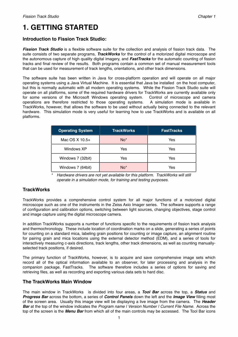
The main window in TrackWorks is divided into four areas, a Tool Bar across the top, a Status and Progress Bar across the bottom, a series of Control Panels down the left and the Image View filling most of the screen area. Usually this image view will be displaying a live image from the camera. The Header Bar at the top of the window indicates the Program name | Version Number | Current File Name. Across the top of the screen is the Menu Bar from which all of the main controls may be accessed. The Tool Bar icons

Fission Track Studio! Chapter 1

1

are shortcuts to the most useful functions which will mostly be covered in detail in later sections. Hovering the mouse over a toolbar item causes a description of its function to be shown in the tooltip.

File Control buttons in the Tool Bar enable a New file to be set up, an old file to be Opened from disc or the current file saved to disc. These functions are short cuts to some of the items in the File Menu, and operate like similar controls in most software packages. TrackWorks uses a structured data storage file system that is automatically generated when images sets are captured, because of the sheer size of the data required for all the images.

The file system for each sample is controlled by a master xml format file that contains all of the sample information and numerical data, as well as controlling the sub-directories containing all of the images. Details of the directories created may be found in the program Help Files. Opening a New file establishes the master xml file for a particular sample and it is important that this be set up in a new directory/folder for that particular sample, as all sub-directories are assigned the same names, such as Grain01, Grain02 etc. Open will open a previously saved xml file, and Save will update a file at any time.

The Image View shows a live image from the digital microscope camera and also displays other information in various overlays, such as a scale bar, a central cross hair, a user definable grid, and various measurement data. A useful feature of the Image View is that the mouse can be used to move around the local area. Clicking at any point in the Image View will bring that point to the centre, and the mouse scroll wheel can be used for fine focussing of the image. The scales of these movements are automatically adjusted for the currently selected objective. These functions are detailed in chapter 3.

The Go To Panel enables any x,y,z coordinate set to be entered and moved to by pressing the Go button. Alternatively, this panel will display the current x,y,z position of the microscope stage by pressing Get.

The Coordination Panel includes tools for setting the positions of two permanent marks on a slide that provide a permanent frame of reference. Once these locations have been set, as described in chapters 4 and 5, all position details can be recalled at a later time, or accessed on another instrument.

The Camera Panel, provides real time controls for the current exposure of the digital camera, and the camera resolution to be selected. A camera exposure in milliseconds can be set by typing a number into the box, or by pressing the up and down arrows which rapidly vary the exposure in 10 ms increments.

The small Enlarge/Reduce arrows under the Camera Panel may be used to collapse or expand the top three panels to make more room for the Grain panel below. A similar set of arrows to the right of the Go To panel allows the whole side bar to be collapsed to make more room for the Image Window.


2

The Grain List panel is an important area that shows a table of all of the currently marked grain locations. When using the EDM, this list shows a parallel set of cells for the corresponding mica positions. A series of control buttons are arranged across the bottom of the Grain List. Grains are added to the list by moving to a suitable position using the microscope controls and pressing the Add button. Once the grains are marked it is possible to move to any one of them simply by double-clicking on its cell in the Grain List, or by selecting it and pressing Go To. Other functions are detailed in chapter 5.

The TrackWorks Menu Bar

The Menu Bar gives access to various settings options, and initiates various actions available in the operation of TrackWorks. Details of these may be found in the online Help files, which are opened by selecting Help under the Windows Menu. The various settings required are also explained mainly in the relevant chapters 3 and 7.

FastTracks

FastTracks is designed to open image sets that have been captured and stored by TrackWorks, and to provide a virtual microscope interface in which these can be examined. The real power and purpose of FastTracks, however, is the automatic fission track counting system that it contains. These image processing algorithms provide a radical new approach to the counting and measurement of fission tracks in natural minerals. The analysis and measurement of fission tracks with this system is now separated from the microscope and can be conducted on a computer anywhere.

FastTracks changes the role of the operator from one of counting all of the tracks manually, to one of reviewing the automatic count results, and correcting these where necessary. The automated counting system and how to use it are described in chapter 8. FastTracks also includes the various track measurement tools that are found in TrackWorks, but in this case they are for use on the captured images.

The FastTracks Main Window

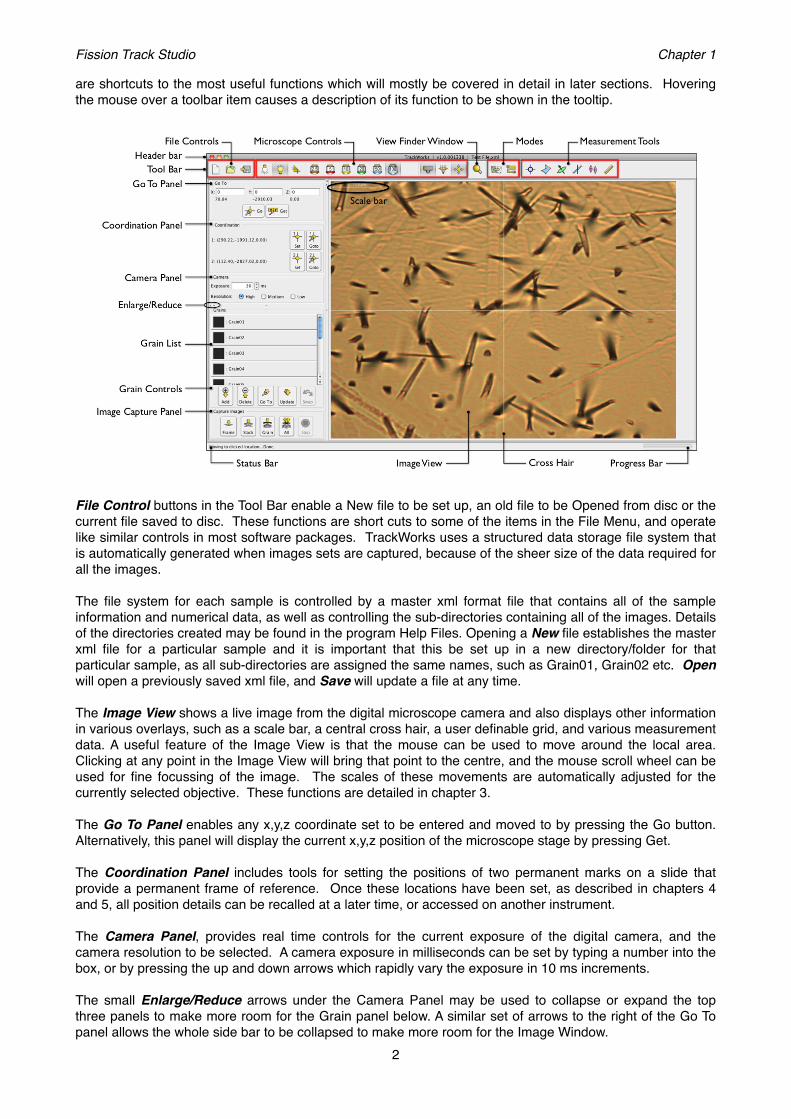
The main window in FastTracks is divided into five areas, as shown, and has many features in common with TrackWorks. The Status Bar and Progress Bar at the bottom have the same functions as in TrackWorks, as have many components of the Tool Bar at the top. The Tool Bar includes File Controls, Measurement Tools and Mode Windows, but with the addition of Automatic Counting Controls. No microscope controls are necessary in FastTracks.

On the left side is the Grain List, which shows all of the grains in the image set. As with TrackWorks, these also include a small thumbnail image of the grain. In the case of EDM samples, the grain list in this case shows either the Grains or the Micas, with two small buttons appearing in the Tool bar to enable selection between the two.

On the right side bar are three panels, the top one controlling the various images and layers that may be placed in the overlay on the central Image View, giving a range of viewing options, not possible with a real microscope. The middle panel summarizes the count results for the currently selected grain (or mica), and the lower panel shows the same results for the entire batch.


3

The Image View window shows as its base layer the image stack captured in transmitted light. This stack can be focused by using the mouse scroll wheel, or by dragging the slider across the bottom of the image. The reflected light image can be overlaid over this image and its transparency set using the relevant slider in the Overlay Controls panel. The reflected light image can be toggled on and off using a right-click of the mouse or by selecting and deselecting it with the button in the Overlay Controls. These options give the operator a complete view of the fission tracks as they would be observed under the microscope.

A left-click of the mouse in the Image View will superimpose the counting results from the automatic counting once this has been carried out. A counting grid may also be overlaid to assist in scanning across the image for any errors in the automatic count results. This grid, unlike that in the real microscope, can be of a variable number of squares and colours, selected in the Overlay Controls panel. The area of counting may be restricted to a polygonal or rectangular Region of Interest (RoI), which is used to select the actual area for counting and remove any undesirable features of the field of view. This RoI can be quite complex to avoid features such as cracks and inclusions, and FastTracks always keeps track of the actual area being counted. Again this is much more flexible than what can be conveniently carried out using a real microscope.

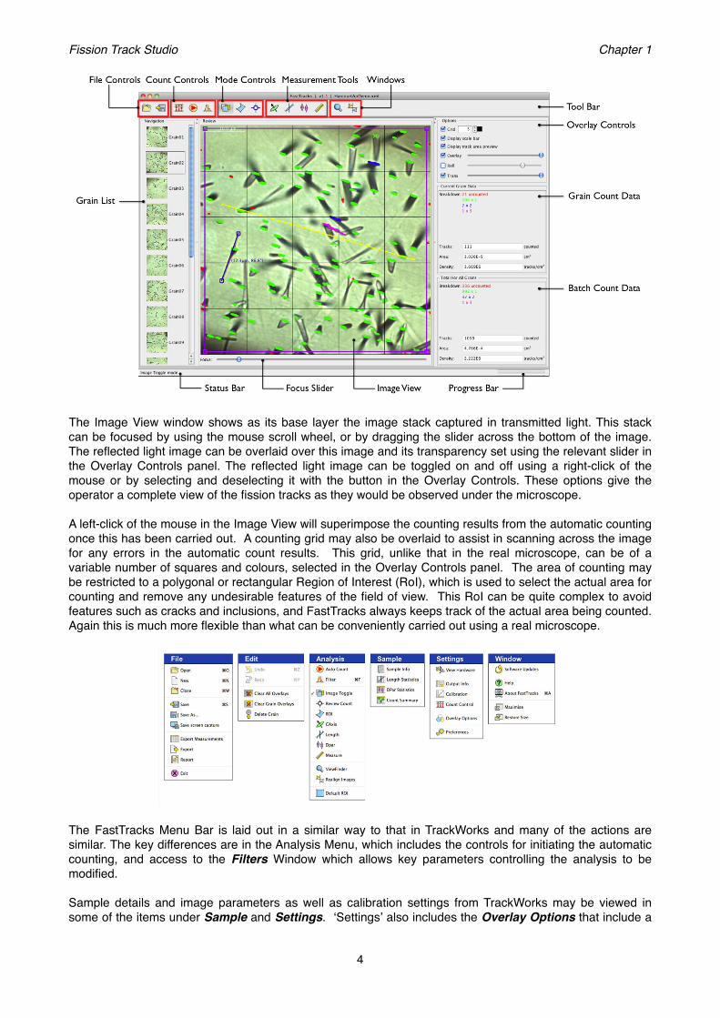
The FastTracks Menu Bar is laid out in a similar way to that in TrackWorks and many of the actions are similar. The key differences are in the Analysis Menu, which includes the controls for initiating the automatic counting, and access to the Filters Window which allows key parameters controlling the analysis to be modified.

Sample details and image parameters as well as calibration settings from TrackWorks may be viewed in some of the items under Sample and Settings. ʻSettingsʼ also includes the Overlay Options that include a


4

number of important settings controlling appearance of the various overlays and a selection of different cursors for use on screen.

Various actions and options in the fastTracks Menu bar are explained in more detail in chapter 8, and also in the online Help files, accessed by selecting ʻHelpʼ in the Window menu.

Updating TrackWorks and FastTracks

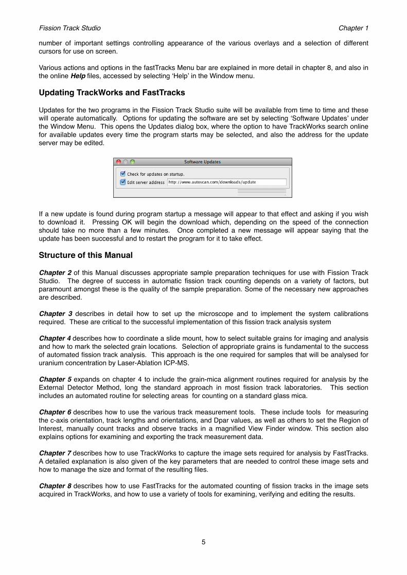
Updates for the two programs in the Fission Track Studio suite will be available from time to time and these will operate automatically. Options for updating the software are set by selecting ʻSoftware Updatesʼ under the Window Menu. This opens the Updates dialog box, where the option to have TrackWorks search online for available updates every time the program starts may be selected, and also the address for the update server may be edited.

If a new update is found during program startup a message will appear to that effect and asking if you wish to download it. Pressing OK will begin the download which, depending on the speed of the connection should take no more than a few minutes. Once completed a new message will appear saying that the update has been successful and to restart the program for it to take effect.

Structure of this Manual

Chapter 2 of this Manual discusses appropriate sample preparation techniques for use with Fission Track Studio. The degree of success in automatic fission track counting depends on a variety of factors, but paramount amongst these is the quality of the sample preparation. Some of the necessary new approaches are described.

Chapter 3 describes in detail how to set up the microscope and to implement the system calibrations required. These are critical to the successful implementation of this fission track analysis system

Chapter 4 describes how to coordinate a slide mount, how to select suitable grains for imaging and analysis and how to mark the selected grain locations. Selection of appropriate grains is fundamental to the success of automated fission track analysis. This approach is the one required for samples that will be analysed for uranium concentration by Laser-Ablation ICP-MS.

Chapter 5 expands on chapter 4 to include the grain-mica alignment routines required for analysis by the External Detector Method, long the standard approach in most fission track laboratories. This section includes an automated routine for selecting areas for counting on a standard glass mica.

Chapter 6 describes how to use the various track measurement tools. These include tools for measuring the c-axis orientation, track lengths and orientations, and Dpar values, as well as others to set the Region of Interest, manually count tracks and observe tracks in a magnified View Finder window. This section also explains options for examining and exporting the track measurement data.

Chapter 7 describes how to use TrackWorks to capture the image sets required for analysis by FastTracks. A detailed explanation is also given of the key parameters that are needed to control these image sets and how to manage the size and format of the resulting files.

Chapter 8 describes how to use FastTracks for the automated counting of fission tracks in the image sets acquired in TrackWorks, and how to use a variety of tools for examining, verifying and editing the results.


5

Online Help Files

Comprehensive online Help files are included in both TrackWorks and FastTracks, accessible from the Window menu in each. The complete Help files are included as Appendices to this Manual in chapters 9 and 10.


6

2. SAMPLE PREPARATION FOR AUTOMATED ! FISSION TRACK COUNTINGIntroduction:

Automated counting of fission tracks, especially when combined with laser-ablation ICP-MS for direct analysis of uranium, requires a somewhat different approach to sample preparation to that used with conventional fission track dating techniques. The following describes some of the procedures that we have found effective in the Fission Track Laboratory at the University of Melbourne. These notes are not exhaustive but are offered as a guide to assist getting started with automated fission track counting.

Most of the methods described here are explicitly for making grain mounts of apatite in epoxy on glass slides. However many of the techniques will also be suitable for processing zircons, or other minerals. As always, some experimentation will be required to adapt the suggested procedures to your local conditions.

For the greatest success in automatic counting of fission tracks it is essential that sample preparation be carried out to the highest standards. Many of the polishing practices and shortcuts that have served well in fission track mount preparation over many years are no longer suitable for the new automated imaging and analysis procedures. The aim in mount preparation for automated counting is to produce completely flat and horizontal polished surfaces of the highest quality, with as few fractures, polishing scratches or other defects as possible. While the new imaging and automatic counting methods are able to discriminate tracks from most of these defects, the methods will clearly work best where they are minimized, or even eliminated. It follows, therefore, that careful attention to detail in sample preparation will produce the best outcomes.

Polishing defects and their causes

There are many different reasons why a polished grain mount may end up with a less than satisfactory polished surface, and, in some cases, these may combine to give a result that is almost unusable. For automated counting it is important that care be taken at every stage of mount preparation, to give the best quality polished surface.

Contributing factors to poor polishing results may include the following:• cracking of grains induced by rock crushing• inadequately mixed or cured resins• grain shatter during grinding• grinding the grains too thinly• contaminated polishing laps• production of excessive surface relief

Few of these factors have received systematic study but the following notes will include advice on how to minimise their effects and ensure the best quality results. For the first of these, it is not really known to what degree the common cracks and cleavage fractures observed in apatites are simply an inherent feature of the grains, or are induced during crushing. Certainly the presence of such cracks varies significantly from sample to sample, so it is likely that some, at least, are a geological characteristic of the grains, but it is equally plausible that some may be induced by mechanical crushing. The advent of high voltage pulsed fragmentation (SelFrag) methods may provide an important new opportunity to test this possibility, and perhaps to release apatites from their host rocks with less cracking.

Grain size and sieving:

The range of grain sizes present in a mineral separate depends on a variety of factors, and is highly variable. However in any particular separate, the largest grains will generally be the most suitable for providing large clear areas for imaging and analysis. It may therefore be appropriate to sieve the separate to extract the most suitable grain size range for mounting. Some labs carry out sieving to produce various size fractions prior to mineral separation, but it is difficult to know at that stage in which size fraction the best grains will occur. It is often more useful to make the separation on unsized material and then to sieve the final concentrate once it can be seen what size range is present.


7

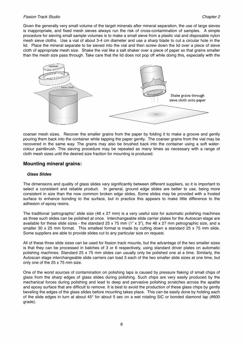
Given the generally very small volume of the target minerals after mineral separation, the use of large sieves is inappropriate, and fixed mesh sieves always run the risk of cross-contamination of samples. A simple procedure for sieving small sample volumes is to make a small sieve from a plastic vial and disposable nylon mesh sieve cloths. Use a vial of about 3-4 cm diameter and use a sharp blade to cut a circular hole in the lid. Place the mineral separate to be sieved into the vial and then screw down the lid over a piece of sieve cloth of appropriate mesh size. Shake the vial like a salt shaker over a piece of paper so that grains smaller than the mesh size pass through. Take care that the lid does not pop off while doing this, especially with the

coarser mesh sizes. Recover the smaller grains from the paper by folding it to make a groove and gently pouring them back into the container while tapping the paper gently. The coarser grains from the vial may be recovered in the same way. The grains may also be brushed back into the container using a soft water-colour paintbrush. This sieving procedure may be repeated as many times as necessary with a range of cloth mesh sizes until the desired size fraction for mounting is produced.

Mounting mineral grains:

Glass Slides

The dimensions and quality of glass slides vary significantly between different suppliers, so it is important to select a consistent and reliable product. In general, ground edge slides are better to use, being more consistent in size than the now common broken edge slides. Some slides may be provided with a frosted surface to enhance bonding to the surface, but in practice this appears to make little difference to the adhesion of epoxy resins.

The traditional ʻpetrographicʼ slide size (46 x 27 mm) is a very useful size for automatic polishing machines as three such slides can be polished at once. Interchangeable slide carrier plates for the Autoscan stage are available for these slide sizes - the standard 25 x 75 mm (1” x 3”), the 46 x 27 mm petrographic size, and a smaller 30 x 25 mm format. This smallest format is made by cutting down a standard 25 x 75 mm slide. Some suppliers are able to provide slides cut to any particular size on request.

All of these three slide sizes can be used for fission track mounts, but the advantage of the two smaller sizes is that they can be processed in batches of 3 or 6 respectively, using standard driver plates on automatic polishing machines. Standard 25 x 75 mm slides can usually only be polished one at a time. Similarly, the Autoscan stage interchangeable slide carriers can load 3 each of the two smaller slide sizes at one time, but only one of the 25 x 75 mm size.

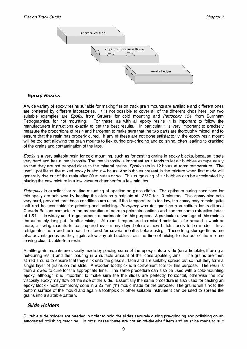
One of the worst sources of contamination on polishing laps is caused by pressure flaking of small chips of glass from the sharp edges of glass slides during polishing. Such chips are very easily produced by the mechanical forces during polishing and lead to deep and pervasive polishing scratches across the apatite and epoxy surface that are difficult to remove. It is best to avoid the production of these glass chips by gently beveling the edges of the glass slides before mounting takes place. This can be easily done by holding each of the slide edges in turn at about 45° for about 5 sec on a wet rotating SiC or bonded diamond lap (#600 grade).


8

Epoxy Resins

A wide variety of epoxy resins suitable for making fission track grain mounts are available and different ones are preferred by different laboratories. It is not possible to cover all of the different kinds here, but two suitable examples are Epofix, from Struers, for cold mounting and Petropoxy 154, from Burnham Petrographics, for hot mounting. For these, as with all epoxy resins, it is important to follow the manufacturers instructions exactly to get the best results. In particular it is very important to precisely measure the proportions of resin and hardener, to make sure that the two parts are thoroughly mixed, and to ensure that the resin has properly cured. If any of these are not done satisfactorily, the epoxy resin mount will be too soft allowing the grain mounts to flex during pre-grinding and polishing, often leading to cracking of the grains and contamination of the laps.

Epofix is a very suitable resin for cold mounting, such as for casting grains in epoxy blocks, because it sets very hard and has a low viscosity. The low viscosity is important as it tends to let air bubbles escape easily so that they are not trapped close to the mineral grains. Epofix sets in 12 hours at room temperature. The useful pot life of the mixed epoxy is about 4 hours. Any bubbles present in the mixture when first made will generally rise out of the resin after 30 minutes or so. This outgassing of air bubbles can be accelerated by placing the new mixture in a low vacuum chamber for a few minutes.

Petropoxy is excellent for routine mounting of apatites on glass slides. The optimum curing conditions for this epoxy are achieved by heating the slide on a hotplate at 135°C for 10 minutes. This epoxy also sets very hard, provided that these conditions are used. If the temperature is too low, the epoxy may remain quite soft and be unsuitable for grinding and polishing. Petropoxy was designed as a substitute for traditional Canada Balsam cements in the preparation of petrographic thin sections and has the same refractive index of 1.54. It is widely used in geoscience departments for this purpose. A particular advantage of this resin is the extremely long pot life after mixing. At room temperature the mixed resin lasts for around a week or more, allowing mounts to be prepared over many days before a new batch needs to be made. In a refrigerator the mixed resin can be stored for several months before using. These long storage times are also advantageous as they again allow any air bubbles from the time of mixing to rise out of the mixture leaving clear, bubble-free resin.

Apatite grain mounts are usually made by placing some of the epoxy onto a slide (on a hotplate, if using a hot-curing resin) and then pouring in a suitable amount of the loose apatite grains. The grains are then stirred around to ensure that they sink onto the glass surface and are suitably spread out so that they form a single layer of grains on the slide. A wooden toothpick is a convenient tool for this purpose. The resin is then allowed to cure for the appropriate time. The same procedure can also be used with a cold-mounting epoxy, although it is important to make sure the the slides are perfectly horizontal, otherwise the low viscosity epoxy may flow off the side of the slide. Essentially the same procedure is also used for casting an epoxy block - most commonly done in a 25 mm (1”) mould made for the purpose. The grains will sink to the bottom surface of the mould and again a toothpick or other suitable instrument can be used to spread the grains into a suitable pattern.

Slide Holders

Suitable slide holders are needed in order to hold the slides securely during pre-grinding and polishing on an automated polishing machine. In most cases these are not an off-the-shelf item and must be made to suit


9

the particular slide format being used. A simple and effective method for holding the slides during these procedures is to make a cylindrical aluminium block that will fit into a standard driver plate on the pressure and rotation head of the polishing machine. A recess is cut into the surface of the block into which the wet slide is held by surface tension. A hole drilled through the block near one corner enables a rod to be inserted to help remove the slide from the holder. It is important that such blocks are precisely made to fit both the driver plate and the slide type being used without too much play so that they are held firmly in the mounting block during polishing.

In the example shown the slide should fit precisely into the recess with a tolerance of only about 50 µm. This means that the slide sizes should be highly consistent and that the blocks are accurately made to fit that particular size. If a larger tolerance is allowed it is likely that the glass slides will produce small chips as they are moved forcefully from side to side in the block during polishing. This will contaminate the polishing laps and seriously degrade the quality of the resulting mounts.

The blocks are made to fit within the driver plate of the polishing machine The holes in the plates come in various sizes and numbers. Struers make plates with three 61 mm diameter holes or six 41 mm holes, which fit mounting blocks that comfortably accommodate 46 x 27 mm and 30 x 25 mm slides sizes, allowing batch processing of three or six at one time. The tolerance between the blocks and the driver plates does not have to be so close, and block diameters about 0.5 mm smaller than the holes are suitable. Such blocks are easily made by local workshops to fit the dimensions of the particular mounting scheme adopted.

Pre-grinding:

The pre-grinding stage is one of the most important as it is often here that otherwise high-quality mounts are damaged, and no amount of polishing can make up for this. The purpose of pre-grinding is to grind the surface of the mount down to expose the grains, and to establish a flat surface parallel to the underlying slide in preparation for polishing. Pre-grinding may include several steps usually involving controlled down-cutting on a #600 grade SiC paper or comparable resin-bonded diamond lap (eg Struers MD Piano) under running water. An even coarser (eg #320 grade) stage may be used first and the surface is usually finished in preparation for polishing at #1200 grade.

The rate of down-cutting decreases with the grain size of the grinding lap, so it follows that the form of the surface will be largely established at the earlier, coarser grades. It is at this stage that it is particularly important to establish a flat surface that is as near as possible parallel to the underlying glass surface. Practice varies as to the amount of epoxy to use on a slide mount, but experience has shown that using more, rather than less, epoxy is useful because it is easier to control ʻwedgingʼ of the mount during pre-grinding. Wedging occurs when the surface of the mount is at an angle to the glass slide surface usually leading to feathering and over-grinding of one edge of the mount. The consequence is that grains near that edge are ground too thin, whereupon they tend to crack up and fall out to contaminate the laps during


10

polishing. A small area of epoxy (<15 mm across) on a slide is much more prone to wedging during pre-grinding than a larger area 20-30 mm across.

A useful procedure to establish a perfectly flat and parallel surface is to use an automated cut-off machine such as the Struers Accutom. This can be used either with a fine diamond saw blade or a diamond cup wheel of various grades. The diamond cup wheel can be very accurately controlled to produce a precisely flat surface at any desired distance above the glass slide. Cutting this surface at 250 µm above the slide surface is an excellent thickness without actually exposing the grains in most samples. The diamond cup wheel is particularly aggressive and tends to shatter the grains it comes in contact with, so it is important to keep the thickness just enough to leave the grains covered. However, establishing a flat surface at this stage allows for controlled down cutting with a #600 grade and finishing with a #1200 resin-bonded diamond lap without wedging. The resin-bonded diamond laps are excellent for grinding a surface through the grains without further cracking. The same effect can be achieved by hand on rotating wet SiC paper laps, but this requires considerable skill to avoid wedging.

Sample Polishing:

Mineral mounts should be produced with no, or at least minimal, surface relief. In practice this means carrying out polishing entirely with diamond polishing compounds and the most accurate and reproducible results are obtained using an automated polishing machine. Alumina and Colloidal Silica slurries should not be used at all as they result in significant surface relief being produced due to the relative hardness difference between the mineral grains and the epoxy mount. Diamond compounds minimize relief production because diamond is relatively so much harder than either the grains or the epoxy mount.

Pre-grinding should be followed by polishing using an automated polishing machine that accurately and consistently controls the parameters of pressure, rotation speed, polishing time and lubricant supply rate. The best results are obtained using a closely spaced sequence of diamond polishing compounds on a suitable rotating cloth lap (eg Struers MD-Dac). Polishing is then carried out using 6 µm, 3 µm, and then 1 µm diamond compounds on cloth laps with 5 Nt pressure for one sample at 150 rpm lap speed. With multiple slide holders the pressure is increased proportionately for the number of slides (e.g. 15 Nt for three slides at a time). A final 0.25µm diamond step may be included (using the same kind of cloth lap), although our experience is that this makes little difference to the final result, and may increase surface relief. Each step should only take about 3 minutes if the preparation has been completed adequately at the previous step. The surface should appear optically perfect after the 1 µm stage with no obvious polishing scratches. A good practice is to polish at the 1µm stage until the surface appears perfect, and then continue for as much time again on the same lap. This doubling of the polishing time at the 1 µm stage significantly decreases residual strain in the surface that appears as polishing scratches after etching.


11

Surface Coating

Why is coating needed?

Apatite and muscovite mica have very low surface reflectivities (~5%), unlike some other uranium-enriched accessory minerals such as zircon and titanite. This low reflectivity has a number of deleterious consequences for the automated counting system based on coincidence mapping of reflected and transmitted light images. One minor reason is that the reflected light image requires a much longer exposure time than the transmitted light image. While the automatic exposure is able to compensate for this to some degree, low-light reflected light images tend to be very noisy thereby degrading image quality and possibly introducing artifacts into the processing.

A much more important reason is that the low surface reflectivity makes the reflected light image prone to interference from internal reflections. In apatite, most of the incident light is actually transmitted through the surface and may be returned by reflections from shallow dipping tracks (particularly problematic at high track densities), fractures or crystal faces below the surface. This gives rise to a ʻreflectedʼ light image that actually includes a significant component of transmitted light. This negates the basic principle of coincidence mapping and causes the automatic counting routine to fail. A third, related, problem is that reflections from some shallow-dipping tracks interfere with light reflected from the surface to produce a series of interference bands along their length. These ʻbandedʼ or ʻzebra-stripedʼ tracks can also cause problems for their detection by automatic counting, although this seldom affects more than a few percent of the total number of tracks. For some, the bright first interference maximum overlaps with the dark etch pit of the track entrance in reflected light so that it is not detected. For others, the first interference minimum can be so dark as to appear like a second etch pit in the reflected light image and cause a false count.

We have found two effective solutions to this major problem of internal reflections in low reflectivity minerals, particularly apatite. The first and most generally useful method is to artificially enhance the surface reflectivity of an apatite mount by applying a thin metal coating, usually aluminium. The second is to double-polish the mount, so that both upper and lower surfaces of the grains are parallel. This is effective in many cases but may be impractical as it requires a significant increase in the number of sample preparation steps. Double-polishing is most effective for low to medium track densities, where internal reflections from crystal faces and fractures are the major contributors, but does not work with high track densities where internal reflections from the tracks themselves are the main problem. Surface coating is effective across all track densities.

Mica surfaces also benefit from coating but the much more uniform nature of the substrate means that internal reflections are seldom much of a problem in this mineral. Reasonable automatic counting results may be obtained from micas even without surface coating.

Vacuum coating

A suitable surface coating can be achieved using a vacuum coating unit, such as those commonly used for sample preparation for Scanning Electron Microscopy. A turbo-pumped coating unit is required to achieve the high vacuum necessary for evaporation of metals from an incandescent filament. The coating is applied using a small amount of aluminium foil placed in a tungsten basket in the vacuum chamber. Ordinary 13 µm thick cooking foil is a suitable source allowing simple control of the amount of Al used by measuring the area of the foil. The measured amount (typically 1.0 cm2) is screwed up into a small ball, placed into the filament basket and the pump-down sequence initiated. Once a high vacuum has been achieved, typically in about 5 minutes, evaporation can begin by gently turning up the filament power. When turning up the power to the filament it is important to do this slowly until the small foil ball has melted onto the filament at a red heat. Turning the power up too quickly usually causes the foil ball to jump out of the basket, so that no coating is possible. Once the foil has melted and spread over the tungsten coils the power level can be turned up until the filament is incandescent.

The coated surface should ideally produce an enhanced reflectivity such that the exposure required for the reflected light image is roughly comparable to that for the transmitted light image. Too thick a coating and the transmitted light image will be degraded and too thin a coating and the internal reflections and banded tracks will still be a problem. Some coating units are fitted with a piezo crystal thickness monitor located beside the sample. Using the thickness monitor, the ideal thickness of Al deposited at the sample surface is


12

about 5-7 nm, which gives optimum enhancement of the surface reflectivity with only minimal reduction in transmissivity.

Some experimentation will be required to get the thickness right for any given coating unit. Two methods have proved useful for controlling the thickness of the film. One is to control the amount of Al placed in the basket and evaporate this entirely each time. We have found that completely evaporating 0.5 cm2 of foil at a distance of 9 cm from the sample produces a coating of about the right thickness. The second is to place an excess of aluminium into the tungsten basket and to control the amount using a mechanical shutter, available on some coating units. With experience this can be done by timing the opening of the shutter, or by monitoring the increasing thickness on a thickness meter, if available.

To become familiar with the most suitable thickness of coating, it is best to practice on a blank slide. The thickness is easier to judge if one end of the slide is shielded so that you can see the contrast between uncoated and coated slide. In this way a set of reference slides with different coating thicknesses can be produced, allowing a quick visual comparison to be made with the results from subsequent experiments. The coated slide should look something like a neutral density filter in terms of its light transmission – a similar light transmission to a 50% neutral density filter, or a polarizing filter, is about what is needed – probably a bit less, and certainly no darker than these.

One advantage of using aluminium for the metal coating is that is can very easily be removed by immersing the coated mount in a dilute solution of NaOH for 20-30 sec, if this should be necessary. A possible disadvantage is that over time (weeks to months) some degradation of the coating may occur due to oxidation producing a patchy and uneven surface. A similar NaOH solution can be used periodically to remove the buildup of aluminium on the glass vacuum chamber, so that the filament can be seen during evaporation. Alternatively the inside of the glass chamber may be rubbed down with a tissue after each run so that a clear window is left to monitor the progress of each evaporation experiment. The vacuum deposited coatings are quite fragile, so care must be taken to only handle slides by their edges after they have been coated.

Gold coatings also produce a suitable enhancement of surface reflectivity but can only be removed by very light re-polishing of the surface. This is likely to have some effect on the track openings at the surface, but in routine operation there should be no necessity to remove the coating. Gold coatings can also be produced by sputter coating units which may be more easily controlled than evaporative coaters. Coating may not be required for zircon and titanite (and possibly monazite), but no experimental results are yet available for these minerals.

Double Polished Mounts

Double polished mounts also produce acceptable results from automatic counting in many cases. These can be produced by first mounting the apatite grains in an epoxy block using a standard 25 mm diameter cylindrical mould and a cold-setting epoxy, such as Epofix. The grains settle to the bottom of the mould and can be spread out into a suitable pattern, as for mounting on a slide. After the epoxy has set, the surface of the block can be ground and polished to expose the grains, and then remounted face-down on a glass slide. It is advisable to again use a cold-setting epoxy for this purpose as differential expansion of the various components can cause problems with hot setting resins at this stage, including breakage of the slide. The block is then reduced in thickness using a cut-off saw and the new surface ground and polished to expose the other side of the grains. In this way grains in the mount have a plate-like form and internal reflections are largely removed. This sequence is illustrated below.


13

It takes significantly longer to make these double polished mounts compared to normal slide mounts and the technique is really only practical for larger grain sizes, but the results can be excellent. The method is also unsuitable for grains with high spontaneous track densities as the problem of internal reflections in such cases is largely caused by the tracks themselves.

Re-cementing mounts for LA-ICP-MS Analysis

One problem that arises when using laser ablation ICP-MS analysis for uranium is that a significant fraction of the grains is lost by jumping out of the mount or cracking up under the laser beam. This does not happen with unetched grains so it appears the etching process loosens the grains in the mount by etching out around the grain boundary. This effect is exacerbated by using a large laser beam diameter (>40 µm) and is minimised by small beam diameters of 20 µm or less. Even so, it is still possible to lose around 20% of grains this way, and for larger beam diameters the fraction lost can be as high as 50%. Clearly this rate of loss is unacceptable, but it is possible to solve the problem by a simple re-cementing procedure using ʻSuperglueʼ (cyanoacrylate) adhesive1. The cement will obviously obscure the details of the tracks, so it is essential that all images have been captured on the coated surfaces before it is applied.

The first step is to squeeze a small drop of Superglue onto the surface of the etched fission track mount after the track images have been acquired. This drop is then spread thinly and evenly across all of the exposed grains on the surface using a small square of teflon sheet as a spreader. We have successfully used a small (~1x1 cm) square of FEP teflon for this purpose, holding the teflon spreader in a pair of forceps. Any excess superglue can be wiped over the edge of the slide onto a tissue underneath. Once the glue is dry any excess


14

1 IMPORTANT: Follow all of the precautions indicated on the superglue tube or packaging and take care not to get any of the adhesive on the skin or eyes as it will stick on contact. However if some does get onto your skin then it can be removed easily using acetone. It is a good idea to have some acetone nearby just in case.

on the side or underneath the slide can be removed with a sharp blade or with a tissue moistened with acetone.

In this way it is possible to spread the superglue into fractures and grain boundaries but leave almost no excess on the surface. Initially, we tried cleaning up any remnant superglue on the surface by lightly polishing on a 0.25 µm diamond lap, but this is usually not necessary as any residual thin film provides no impediment to the laser probe. With practice the re-cementing can be carried out with almost no residue left on the surface. One necessary caution is to ensure that any re-coordination marks on the slide are not covered and obscured by the superglue.

Re-coordination Marks

A set of precise reference marks need to be added to each mount so that the coordinates of analysed grains can be transferred to the stage system of another instrument such as a Laser-Ablation ICP-MS or an Electron Microprobe. Similarly for an EDM mount it is important to have reference marks on the slide, so that the slide can be reinserted on the stage at a later time and stored locations recalled from file. The current automated Fission Track system uses two ʻRe-coordinationʼ points for this purpose.

A variety of methods have been used for marking reference points on a fission track slide. These consist of either scribing or cementing a suitable marker to the slide surface. The simplest method is scribing a mark on the glass or epoxy surface with a diamond scriber or other hard point. Such scribed marks suffer from being not very reproducible and are rather large and irregular when observed under a microscope. They are therefore not the most suitable for use as precise location points. If a laser ablation system is available, the laser itself may be used to scribe a precise location mark on the slide surface using a beam width as small as 5µm.

Perhaps the most precise method of making reference marks is to glue one or more electron microscope grids to the surface of the slide., an approach now used in a number of laboratories. One type of grid that is widely used consists of a 3mm diameter copper disc with an interior grid and a small letter “A” at the centre. This is the Athene 200 mesh, centre mark grid. These copper electron microscope grids are very easy to locate on the slide and offer a very precise and reproducible location mark at the centre of the disc.

The exact centre of the circular grid can be easily identified as being at the midline of the central cross hairs of the grid, highlighted in red in the illustration. This central point in the letter “A” can be used as an exactly repeatable reference location to provide an internal reference point on the slide itself. Note that for this particular grid, the exact centre of the circular grid is either in the middle of the cross-bar of the “A”, as shown, or in the middle of the triangular gap within the “A”. Many other EM grids patterns are also available which could be used.

Two re-coordination points should be used on each slide. Electron microscope grids can be simply glued to the slide using a small drop of cyanoacrylate cement (Superglue) or epoxy. It is best to use a very small amount of the adhesive - dropping directly from the bottle puts too much glue onto the slide. A simple way to get the right amount is to first squeeze out a drop of superglue onto a blank slide as a palette, and then use a toothpick to transfer a small amount to the actual mount. Spread the glue into a small circle about 2 mm in diameter with the toothpick and then carefully lower the EM grid on top of this using fine-tipped forceps. This works best by lowering one edge of grid down into the glue first and then dropping it so that it settles down neatly onto the surface with the glue spreading by capillary action to the edge of the disc. Again it is


15

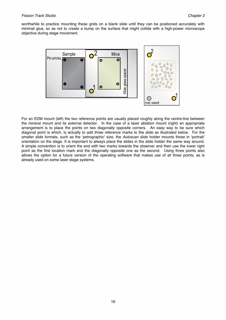
worthwhile to practice mounting these grids on a blank slide until they can be positioned accurately with minimal glue, so as not to create a bump on the surface that might collide with a high-power microscope objective during stage movement.

For an EDM mount (left) the two reference points are usually placed roughly along the centre-line between the mineral mount and its external detector. In the case of a laser ablation mount (right) an appropriate arrangement is to place the points on two diagonally opposite corners. An easy way to be sure which diagonal point is which, is actually to add three reference marks to the slide as illustrated below. For the smaller slide formats, such as the ʻpetrographicʼ size, the Autoscan slide holder mounts these in ʻportraitʼ orientation on the stage. It is important to always place the slides in the slide holder the same way around. A simple convention is to orient the end with two marks towards the observer and then use the lower right point as the first location mark and the diagonally opposite one as the second. Using three points also allows the option for a future version of the operating software that makes use of all three points, as is already used on some laser stage systems.


16

3. SETTING UP AND OPERATING THE MICROSCOPEIntroduction:

TrackWorks is designed to provide a convenient operating environment to control an advanced, fully motorized microscope, such as the Zeiss Axio Imager series, coupled with an Autoscan stage. The software provides control over all of the major microscope functions and the image capture sequence for automated fission track analysis. It is important for the best performance of the Fission Track Studio suite that the microscope is properly adjusted and calibrated.

Microscope Adjustment

It is very important in preparation for digital imaging to ensure that the microscope is correctly adjusted to provide the best possible illumination conditions for image capture. It is worthwhile spending some time with the manufacturerʼs manual for the microscope and become familiar with all of its functions and adjustments. If the microscope is not correctly adjusted then the optical system may be operating at significantly less than its optimal performance, and captured digital images will be poorer in quality.

Modern research microscopes are all equipped with a sub-stage condenser and field and aperture diaphragms required to produce Koehler illumination1 providing the most uniform illumination across the field of view and and the maximum optical resolution for a particular objective lens. For brightfield transmitted light observation the first step in setting up is to ensure that the microscope is properly adjusted with the substage condenser lens at the correct height, properly centred, and having the field stop and condenser aperture diaphragms stopped down to the correct degree to provide Koehler illumination. In reflected light the field diaphragm should be adjusted to be just at the limit of the visible field to reduce glare and maximise contrast in the image. It is important to set up the optimum illumination conditions for the particular objective which is to be used for image capture. Almost always this will be the 100x lens.

Selecting Hardware

The software is able to be configured for various hardware options. These are selected under ʻSelect Devicesʼ in the ̒ Hardwareʼ menu. Choose the appropriate Microscope, Stage and Camera for your particular hardware set up using the pull-down menus under each of these categories. There is also a category for an

ʻOptovarʼ feature, which is a variable magnification changer fitted to some microscopes. The list under ʻOptovarʼ can also include c-mount adaptors of different magnification factors in the c-mount adaptor used to connect the digital microscope camera. A simulated option is also available for Microscope, Stage and Camera, that enables TrackWorks to be used even when the computer is not connected to these hardware items. This is valuable for enabling the user to become familiar with the software and its various functions. The software performs all of its normal functions in Sim mode, simply without a live camera image or actual responses from the microscope and stage.

Microscope Configuration Controls

TrackWorks includes a series of controls for changing the objectives, for switching the illumination between transmitted and reflected light, adjusting the reflector position, controlling the digital camera and


17

1 http://www.olympusmicro.com/primer/anatomy/kohler.htmlhttp://www.zeiss.de/c1256b5e0047ff3f/Contents-Frame/b5a0494cdab43f2ac1256c3e00365e5e

http://www.olympusmicro.com/primer/anatomy/kohler.html

http://www.olympusmicro.com/primer/anatomy/kohler.html

http://www.zeiss.de/c1256b5e0047ff3f/Contents-Frame/b5a0494cdab43f2ac1256c3e00365e5e

http://www.zeiss.de/c1256b5e0047ff3f/Contents-Frame/b5a0494cdab43f2ac1256c3e00365e5e

automatically focussing the image. A range of settings are also available for these functions which are accessed under the ʻHardwareʼ menu.

The group at the left reconfigure the microscope illumination, the centre groups selects the objectives and the right pair controls the live image from the camera and autofocus routine. The left pair toggle between reflected and transmitted light respectively, while the prism symbol ensures that the reflector cube for reflected light operation is positioned correctly.

Illumination Controls

# Select Reflected Light

# Select Transmitted Light

# Position Reflector Cube

Objective Controls

# Select Objective

One objective lens button will be present for each objective installed on the microscope nosepiece. These must be configured using the Objective Settings under the Hardware menu, as described below.

Action Controls

The remaining three microscope control buttons are as follows

# Live Camera Image

The default setting for this control is for the live camera image to be selected, which is the most appropriate setting for most operations. The colour of the cross hair shows the current status: white = live, black = static.

# Autofocus


18

Press this button to select Reflected light observation. The button opens the reflected light shutter and closes that for transmitted light. This option also rotates the reflector into the correct position.

Press this button to select Transmitted light observation. The button opens the transmitted light shutter and closes that for reflected light

Press this button when the reflector to allow reflected light observation is not in the correct position

There is one objective lens button for each objective installed. Press the relevant lens button to rotate that objective into position

Toggles a live image from the digital microscope camera on and off. If the live image is off, the main window displays a static image of the field of view

Operates the autofocus routine on the current field of view, according to the parameters defined in Autofocus Settings Preferences

The Autofocus routine is mostly used during image capture, when the microscope is operating under autonomous control. When the observer is at the microscope it is much faster to simply focus manually, or for fine focus, the mouse scroll wheel may also be used, provided this has been enabled in ʻMicroscope Settingsʼ.

# Movement Control

The movement control button is grouped in the right hand cluster on the tool bar, adjacent to the measurement tools as it is often used in conjunction with these tools. Under movement control using the computer mouse, the stage moves in a click to centre mode. Simply click on any point and that point will move to the centre of the screen. This movement function scales automatically whenever the objectives are changed. The scroll wheel on the mouse can also be used to make fine focus adjustments, and again the amount of focus movement for a given rotation of the scroll wheel is scaled to the particular objective being used.

Hardware Settings

The Hardware menu gives access to various hardware settings, apart from ʻSelect Devicesʼ described above. These include the Camera Control, Objective Settings, Stage Settings and Microscope Settings.

# Camera Control

Some of the camera controls (the current exposure and the resolution) are also displayed in the Camera Panel of the main window. The exposure allows the current exposure of the digital microscope camera, in milliseconds, to be adjusted. To change the exposure, enter a numerical value into the box and press ʻEnterʼ., or press the up and down arrows until the desired value is reached. The arrows increase or decrease the current exposure levels by 10 milliseconds at a time. The Gain is set at 10 by default and it is seldom necessary to change this value. Higher values of the gain may be used but tend to increase the noise levels in the digital images if too high, which is undesirable.

Many digital microscope cameras can be operated in high, medium or low resolutions and in some the frame rate increases at the lower resolutions, which may be useful for adjusting the focus or moving the stage while looking at the screen. However it is usually best to capture digital images using the high resolution setting.

Some cameras, notably the Olympus SIS family, also enable the colour balance of the camera to be adjusted. This is useful for correcting colours in the image due to the colour temperature of the lamp, for example. The adjustments are made by adjusting Red, Green and Blue values in the dialog box.

# Stage Settings

The direction the stage moves in response to input from the joystick, or mouse commands can be set in this panel. Individual operators vary in their preferred movement modes and different microscope optics make movements in either x or y directions, or both, that appear to be in the opposite directions to the actual movements. Being able to invert the movement direction in response to commands makes the microscope more intuitive to use for different observers. Choose + or - options for x, y and z movements in the Stage Settings panel to adjust the movement directions according to your own preferences.


19

This is the default option when moving the stage. When this is selected the mouse can be used to control stage movement in addition to using the joystick.

Camera control sets the exposure, gain and resolution for the digital microscope camera.

Sets the default movement directions for stage x, y and z directions, and two stage movement parameters

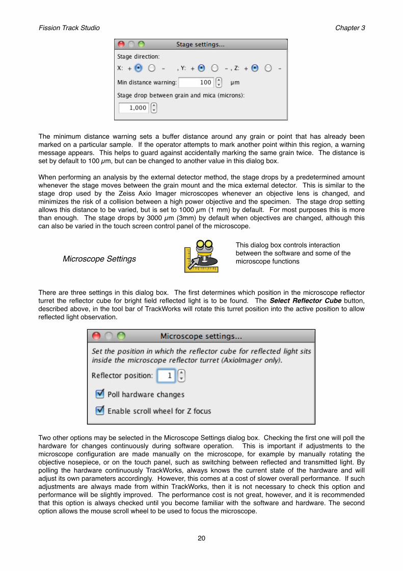
The minimum distance warning sets a buffer distance around any grain or point that has already been marked on a particular sample. If the operator attempts to mark another point within this region, a warning message appears. This helps to guard against accidentally marking the same grain twice. The distance is set by default to 100 µm, but can be changed to another value in this dialog box.

When performing an analysis by the external detector method, the stage drops by a predetermined amount whenever the stage moves between the grain mount and the mica external detector. This is similar to the stage drop used by the Zeiss Axio Imager microscopes whenever an objective lens is changed, and minimizes the risk of a collision between a high power objective and the specimen. The stage drop setting allows this distance to be varied, but is set to 1000 µm (1 mm) by default. For most purposes this is more than enough. The stage drops by 3000 µm (3mm) by default when objectives are changed, although this can also be varied in the touch screen control panel of the microscope.

# Microscope Settings

There are three settings in this dialog box. The first determines which position in the microscope reflector turret the reflector cube for bright field reflected light is to be found. The Select Reflector Cube button, described above, in the tool bar of TrackWorks will rotate this turret position into the active position to allow reflected light observation.

Two other options may be selected in the Microscope Settings dialog box. Checking the first one will poll the hardware for changes continuously during software operation. This is important if adjustments to the microscope configuration are made manually on the microscope, for example by manually rotating the objective nosepiece, or on the touch panel, such as switching between reflected and transmitted light. By polling the hardware continuously TrackWorks, always knows the current state of the hardware and will adjust its own parameters accordingly. However, this comes at a cost of slower overall performance. If such adjustments are always made from within TrackWorks, then it is not necessary to check this option and performance will be slightly improved. The performance cost is not great, however, and it is recommended that this option is always checked until you become familiar with the software and hardware. The second option allows the mouse scroll wheel to be used to focus the microscope.


20

This dialog box controls interaction between the software and some of the microscope functions

Objective Calibration Dialog

The Objective Calibration Dialog box is revealed by selecting ʻHardware>Objective Settingsʼ. This is one of the most important settings panels as it controls the arrangement of objective lenses in the microscope nosepiece, the calibration of each objective for the particular digital camera in use, the alignment of the objectives relative to each other and the default camera exposure settings for each objective. The Objective Calibration Dialog is divided into five different panels corresponding to these functions.

# Objective Settings

Identifying Objective Positions

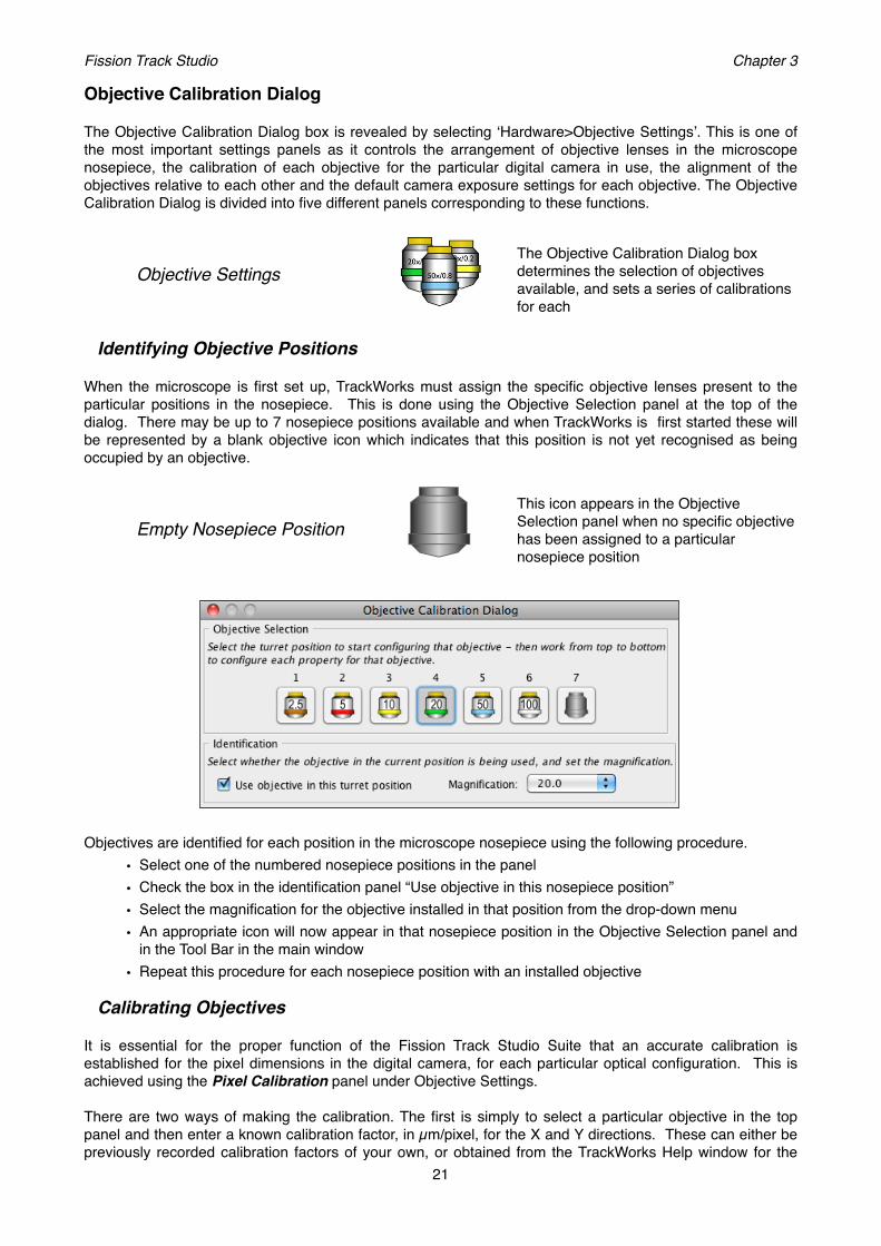
When the microscope is first set up, TrackWorks must assign the specific objective lenses present to the particular positions in the nosepiece. This is done using the Objective Selection panel at the top of the dialog. There may be up to 7 nosepiece positions available and when TrackWorks is first started these will be represented by a blank objective icon which indicates that this position is not yet recognised as being occupied by an objective.

# Empty Nosepiece Position

Objectives are identified for each position in the microscope nosepiece using the following procedure.• Select one of the numbered nosepiece positions in the panel• Check the box in the identification panel “Use objective in this nosepiece position”• Select the magnification for the objective installed in that position from the drop-down menu • An appropriate icon will now appear in that nosepiece position in the Objective Selection panel and

in the Tool Bar in the main window• Repeat this procedure for each nosepiece position with an installed objective

Calibrating Objectives

It is essential for the proper function of the Fission Track Studio Suite that an accurate calibration is established for the pixel dimensions in the digital camera, for each particular optical configuration. This is achieved using the Pixel Calibration panel under Objective Settings.

There are two ways of making the calibration. The first is simply to select a particular objective in the top panel and then enter a known calibration factor, in µm/pixel, for the X and Y directions. These can either be previously recorded calibration factors of your own, or obtained from the TrackWorks Help window for the


21

The Objective Calibration Dialog box determines the selection of objectives available, and sets a series of calibrations for each

This icon appears in the Objective Selection panel when no specific objective has been assigned to a particular nosepiece position

most common cameras in use by the system. These factors are found under Windows>Help> Configuration>Pixel Calibration. They are calculated from the known pixel dimensions for each camera type and the magnification for each particular lens. They are accurate to better than 1%. The calibration factors are automatically recorded for future use when TrackWorks is closed, so it should not be necessary to re-enter the calibrations every time the system is used.

The second method is to carry out a calibration for each objective using a stage micrometer. TrackWorks contains a convenient tool for this purpose. Detailed instructions on how to do this are also contained in the TrackWorks online Help files. The first step is to insert a stage micrometer slide in the stage slide holder. For each objective, focus on the graduations on the slide and make sure that the graduations are precisely aligned with the left and right edges of the image. Adjust the alignment of the graduations by rotating the digital camera on the c-mount adapter.

In the Pixel Calibration panel select the known interval to be measured on the stage micrometer from the drop-down ʻDistanceʼ menu micrometer, such as 100 µm, and press ʻRecordʼ. The measurement tool will now be active and will measure the pixel dimensions between two mouse clicks on the screen image. Simply click on one graduation and then on another and a horizontal line will appear between the two points with its length in pixels beside it. The measurement tool is constrained to move either in the X-axis or the Y-axis on screen. Once drawn, the length of the line can be adjusted by clicking and dragging on one of the handles at each end, or the line can be removed by right-clicking on it and selecting ʻDeleteʼ. Repeat the calibration measurement in this direction as many times as desired across the area of the screen. Twenty or more measurements should provide a stable calibration. The routine will keep a running average of the calibration in µm/pixel and enters the X-calibration factor into the box when ʻSaveʼ is pressed.

Then rotate the camera through 90°, once again taking care that the graduation lines are precisely aligned with the top and bottom edges of the image. Make another series of measurements this time moving the cursor in the vertical direction to calibrate the dimensions in the Y-direction. Once a suitable calibration has been achieved, press ʻSaveʼ to record the final calibration factor for Y.


22

The colour of the calibration lines can be changed to enhance their visibility by selecting the Colour options tab in Preferences>Overlay Options. Simply choose a particular overlay feature (ʻcalibration linesʼ in this case) and a colour selection palette will appear. Click on a new colour and this will become the colour on the screen overlay. A choice of three colour spaces is available: swatches, HSB and RGB.

Objective Offsets

TrackWorks enables you to correct for the small offsets in x, y and z that exist between objective lenses in the nosepiece, such that a particular object at the exact centre of the field of view for one objective is no longer exactly centred or perfectly in focus for another. These offsets are determined using the Objective offsets panel in the Objective Settings Dialog box. Start this procedure by selecting ʻEnable Objective Offsetsʼ.

To record the offsets set a reference point by focussing on a well resolved fine feature using the most powerful objective, usually the 100x, and centering this precisely on the screen cross-hairs. Click on the ʻSet Referenceʼ button. Change to the 50x objective and again centre and focus on the same point. Press ʻSetʼ to record the offsets for this objective. Repeat for the next lowest objective and so on down to the lowest power, and then close then Objective Settings Dialog box. From then on the system will adjust for these offset amounts every time the objective is changed.

Exposure Presets

For each objective and illumination mode it is important to set the correct camera exposure so that captured images will be suitable for image analysis. The current exposure setting for the camera is displayed and may be adjusted, in ʻCamera Panelʼ on the left of the main window. Preset exposure values may also be set for each objective lens for both reflected and transmitted light, and these preset values will be used during automatic control of an image capture sequence. These presets are set using the ʻPresets Exposure Valuesʼ panel in the ʻObjective Settingsʼ Dialog box.


23

To enable this option, first choose the particular objective in the ʻObjective Selection panelʼ at the top of the dialog, or on the main Tool bar, and then select ʻUse preset exposuresʼ. Select an appropriate exposure in the box and this will become the new preset value. Moving the up and down arrows will increase or decrease the current exposure value in 10 ms increments, or a specific value can be typed into the exposure setting box. These changes will operate on the current live image, so a suitable value can be selected for the current sample.

This process is repeated for both reflected and transmitted light to set the preset values for each illumination mode. The camera gain setting may also be set in the same way, although, the default value of 10 is suitable for most purposes.

Saving the Current Settings

Once appropriate calibrations and settings have been set, the current values may be saved as the default settings for future reference. Select Preferences>Defaults and choose the “Select Current Settings as Default” option. This will save the current settings which may then be restored at any time in the future by selecting “Restore Default Settings” in the same Dialog panel. It is highly advisable to do this, so that if the preferences and calibrations are lost for any reason, they can be very simply recovered without having to reset each one individually. It may also be wise to save a backup copy of this file (called ʻdefaults.xmlʼ in the TrackWorks folder) at a different location on the hard disc so that a permanent record of the default values is held in case these are lost.

Inserting a Slide

The first step in preparing for work on a sample mount is to ensure that the slide is correctly inserted into the slide holder. The Autoscan Stage system uses interchangeable slide holders that are held firmly into the x-axis caliper by a powerful magnet. This arrangement has advantages in simplifying the process of changing slides and catering for a variety of slide formats. The slides are held in these carrier plates by pressure on their sides, which means it is possible for the inserted slides to come to rest above the underlying glass carrier plate. This will cause problems for the focus level if the slide is reinserted into the holder for inspection of marked points at a later date, as the focus level is likely to be different to that recorded. It is therefore important to make sure that the slides are firmly pressed down onto the glass plate of the slide

carrier. The correct slide insertion sequence is illustrated. Once the slide, or slides, are inserted, the carrier plate can be slid into place on the stage. Be sure that the carrier is securely fitted into the caliper and that the magnetic catch has engaged. You are now ready to begin observation and image capture.


24

4. Selecting and Marking GrainsTrackWorks can be used either for grain mounts for the LA-ICP-MS method, or paired grain/mica mounts being used for the traditional External Detector Method (EDM). For uranium determination by the LA-ICP-MS method no neutron irradiation is required and therefore a larger grain mount is possible. In addition, only a single track density (for the spontaneous tracks) is required and so the slide marking and grain handling procedure is simpler than for the EDM. The following describes procedures as they apply to the LA-ICP-MS approach sequence.

The steps involved are:

• Slide Coordination

• Selecting suitable grains

• Marking the selected grains

Slide Layout

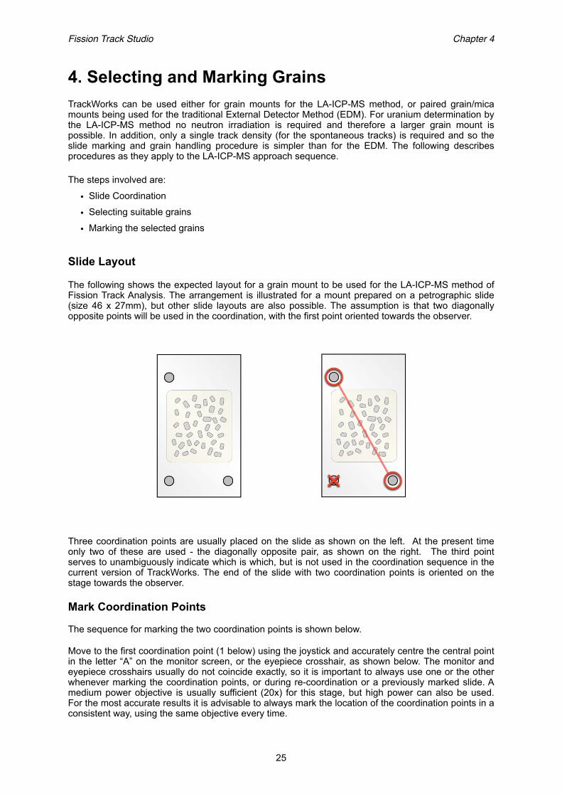
The following shows the expected layout for a grain mount to be used for the LA-ICP-MS method of Fission Track Analysis. The arrangement is illustrated for a mount prepared on a petrographic slide (size 46 x 27mm), but other slide layouts are also possible. The assumption is that two diagonally opposite points will be used in the coordination, with the first point oriented towards the observer.

Three coordination points are usually placed on the slide as shown on the left. At the present time only two of these are used - the diagonally opposite pair, as shown on the right. The third point serves to unambiguously indicate which is which, but is not used in the coordination sequence in the current version of TrackWorks. The end of the slide with two coordination points is oriented on the stage towards the observer.

Mark Coordination Points

The sequence for marking the two coordination points is shown below.

Move to the first coordination point (1 below) using the joystick and accurately centre the central point in the letter “A” on the monitor screen, or the eyepiece crosshair, as shown below. The monitor and eyepiece crosshairs usually do not coincide exactly, so it is important to always use one or the other whenever marking the coordination points, or during re-coordination or a previously marked slide. A medium power objective is usually sufficient (20x) for this stage, but high power can also be used. For the most accurate results it is advisable to always mark the location of the coordination points in a consistent way, using the same objective every time.


25

Mark this point using the ‘set first reference’ button in the Coordination panel in TrackWorks. A dialog box will open called ‘First Reference’ and asking you whether you wish to set the first reference point at the current location. Click ‘Yes’ and then move the stage with the joystick until the second, diagonally opposite, point is exactly centred. Mark this point using the ‘set second reference’ button. Again click ‘yes’ in the ‘Second Reference’ dialog box that opens. The baseline coordination sequence is now complete.

Grain Selection

It is very important that only grains with polished surfaces parallel to their crystallographic c-axes should be selected. This is because the coincidence mapping and multiple correction technique, which is central to the automatic counting procedure, only works successfully for grains with c-parallel surfaces. This is comparable to the procedure used in traditional manual counting methods, but needs to be applied rigorously in the case of automatic counting. The following criteria should be used to select suitable grains:

• Surfaces should display sharp polishing scratches

• Long axes of track etch pits in reflected light should be parallel

The form of track etch pits in reflected light and the appearance of polishing scratches for different orientations of the polished surface relative to the c-axis are illustrated diagrammatically below.


26

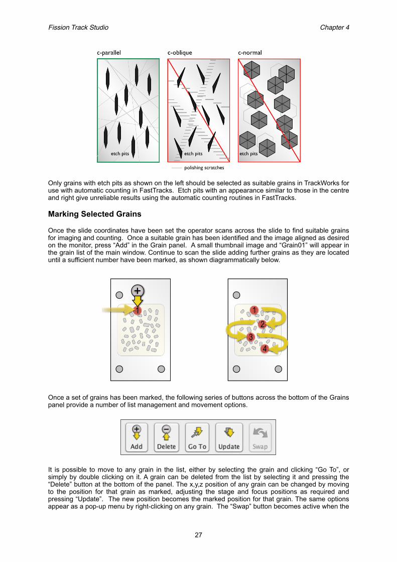
Only grains with etch pits as shown on the left should be selected as suitable grains in TrackWorks for use with automatic counting in FastTracks. Etch pits with an appearance similar to those in the centre and right give unreliable results using the automatic counting routines in FastTracks.

Marking Selected Grains

Once the slide coordinates have been set the operator scans across the slide to find suitable grains for imaging and counting. Once a suitable grain has been identified and the image aligned as desired on the monitor, press “Add” in the Grain panel. A small thumbnail image and “Grain01” will appear in the grain list of the main window. Continue to scan the slide adding further grains as they are located until a sufficient number have been marked, as shown diagrammatically below.

Once a set of grains has been marked, the following series of buttons across the bottom of the Grains panel provide a number of list management and movement options.

It is possible to move to any grain in the list, either by selecting the grain and clicking “Go To”, or simply by double clicking on it. A grain can be deleted from the list by selecting it and pressing the “Delete” button at the bottom of the panel. The x,y,z position of any grain can be changed by moving to the position for that grain as marked, adjusting the stage and focus positions as required and pressing “Update”. The new position becomes the marked position for that grain. The same options appear as a pop-up menu by right-clicking on any grain. The “Swap” button becomes active when the


27

External Detector Method Mode is being used. An additional “Save” option that appears in the pop-up menu allows a new image set for that particular grain to recaptured, below.

Re-coordination of a Slide

After it has been processed, a slide can always be placed back in the slide holder and re-coordinated. Previously marked points can then be recalled by opening the saved file, and repeating the coordination sequence described above under 2. Moving to the two coordination points in turn and selecting the respective “Set Point” buttons will reset the reference frame for that slide to its new position in the slide holder. From then on all previously marked points should be accessible from the grain list, just as they were when the slide was first labelled. Any small adjustments in position that may be needed can be made by moving the stage, refocussing and then pressing update in the Grains panel of the main window.

Export Grain Coordinates

In order to transfer the coordinates of the marked grains into another analytical system, such as a laser ablation stage system for ICP-MS analysis, or an Electron Microprobe, the coordinates need to be exported from TrackWorks. This is done with the “Export DCD…” command under the File menu, which saves the x, y and z coordinates to a disc file for the two Coordination Points and for all grain locations that have been marked. For grains, the coordinates refer to the centre of the marked area.

Enter a suitable file name in the standard file save dialog box that opens, and save the file to a suitable disc location. The file is saved in the DCD format with a .dcd file type extension. There is no header line within the DCD format, so it is very important to use a file name that clearly identifies the sample.

The DCD format is a 9-column Tab-delimited text file designed for import into a number of laser ablation stages. The first two lines of the table are for the coordination points P1 and P2, and assigned the label RecMark (for Re-coordination Mark). This is followed by one line for each grain location that has been marked using the following format.


28

In the example below, only the part highlighted in colour comprises the actual DCD file.

X Y Z Label Name Display Kind Group Element

7126.45 6294.87 2470 RecMark P1 P1 1 1 1-8183.34 -5307.67 2270 RecMark P2 P2 1 1 2-5437.75 127.76 3350 MISCELL GRAIN 1 0 0 0-8057.9 5897.67 3420 MISCELL GRAIN 2 0 0 0

-9925.46 1939.56 2850 MISCELL GRAIN 3 0 0 0-4643.34 1149.8 3360 MISCELL GRAIN 4 0 0 0

The first three columns record x, y and z coordinates in microns. Z may be zero if this is not used by the laser stage. The remaining columns are text labels and information about the marked locations. TrackWorks assigns GRAIN and a sequential number for each marked grain location in columns 5 and 6 ('Name' and 'Display'). The last three columns are not used by TrackWorks for the marked grains.

If desired, the file can be imported into Excel for conversion to another format by changing the filename extension from .dcd to .csv (comma separated values). Some stage systems may require the X and Y columns to be in the reverse order, which can be selected as an option in TrackWorks by selecting “Swap X and Y in DCD export” under “Miscellaneous” in the Preferences Menu.


29


30

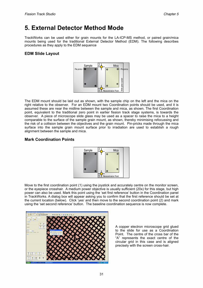
5. External Detector Method ModeTrackWorks can be used either for grain mounts for the LA-ICP-MS method, or paired grain/mica mounts being used for the traditional External Detector Method (EDM). The following describes procedures as they apply to the EDM sequence

EDM Slide Layout

The EDM mount should be laid out as shown, with the sample chip on the left and the mica on the right relative to the observer. For an EDM mount two Coordination points should be used, and it is assumed these are near the midline between the sample and mica, as shown. The first Coordination point, equivalent to the traditional zero point in earlier fission track stage systems, is towards the observer. A piece of microscope slide glass may be used as a spacer to raise the mica to a height comparable to the surface of the sample grain mount, as shown, thereby minimising refocussing and the risk of a collision between the objectives and the grain mount. Pin-pricks made through the mica surface into the sample grain mount surface prior to irradiation are used to establish a rough alignment between the sample and mica.

Mark Coordination Points

Move to the first coordination point (1) using the joystick and accurately centre on the monitor screen, or the eyepiece crosshair. A medium power objective is usually sufficient (20x) for this stage, but high power can also be used. Mark this point using the ‘set first reference’ button in the Coordination panel in TrackWorks. A dialog box will appear asking you to confirm that the first reference should be set at the current location (below). Click ‘yes’ and then move to the second coordination point (2) and mark using the ‘set second reference’ button. The baseline coordination sequence is now complete.


31

A copper electron microscope grid glued to the slide for use as a Coordination Point. The centre of the cross bar of the “A” represents the exact centre of the circular grid in this case and is aligned precisely with the screen cross-hair.

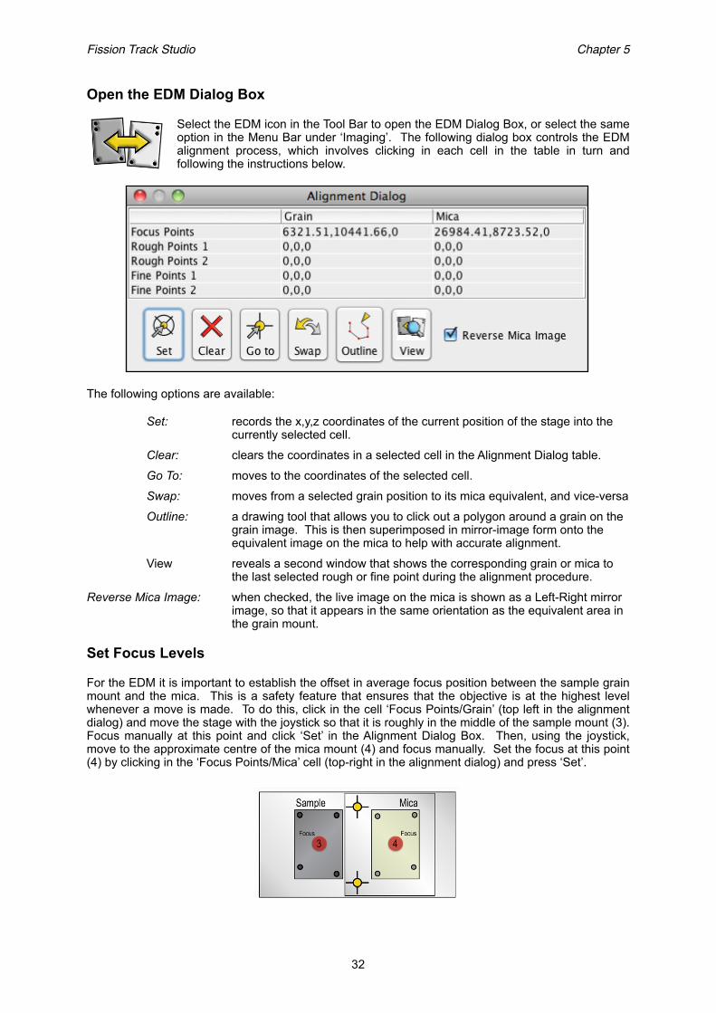
Open the EDM Dialog Box

Select the EDM icon in the Tool Bar to open the EDM Dialog Box, or select the same option in the Menu Bar under ‘Imaging’. The following dialog box controls the EDM alignment process, which involves clicking in each cell in the table in turn and following the instructions below.

The following options are available:

Set: records the x,y,z coordinates of the current position of the stage into the currently selected cell.

Clear: clears the coordinates in a selected cell in the Alignment Dialog table.

Go To: moves to the coordinates of the selected cell.

Swap: moves from a selected grain position to its mica equivalent, and vice-versa

Outline: a drawing tool that allows you to click out a polygon around a grain on the grain image. This is then superimposed in mirror-image form onto the equivalent image on the mica to help with accurate alignment.

View reveals a second window that shows the corresponding grain or mica to the last selected rough or fine point during the alignment procedure.

Reverse Mica Image: when checked, the live image on the mica is shown as a Left-Right mirror image, so that it appears in the same orientation as the equivalent area in the grain mount.

Set Focus Levels

For the EDM it is important to establish the offset in average focus position between the sample grain mount and the mica. This is a safety feature that ensures that the objective is at the highest level whenever a move is made. To do this, click in the cell ‘Focus Points/Grain’ (top left in the alignment dialog) and move the stage with the joystick so that it is roughly in the middle of the sample mount (3). Focus manually at this point and click ‘Set’ in the Alignment Dialog Box. Then, using the joystick, move to the approximate centre of the mica mount (4) and focus manually. Set the focus at this point (4) by clicking in the ‘Focus Points/Mica’ cell (top-right in the alignment dialog) and press ‘Set’.


32

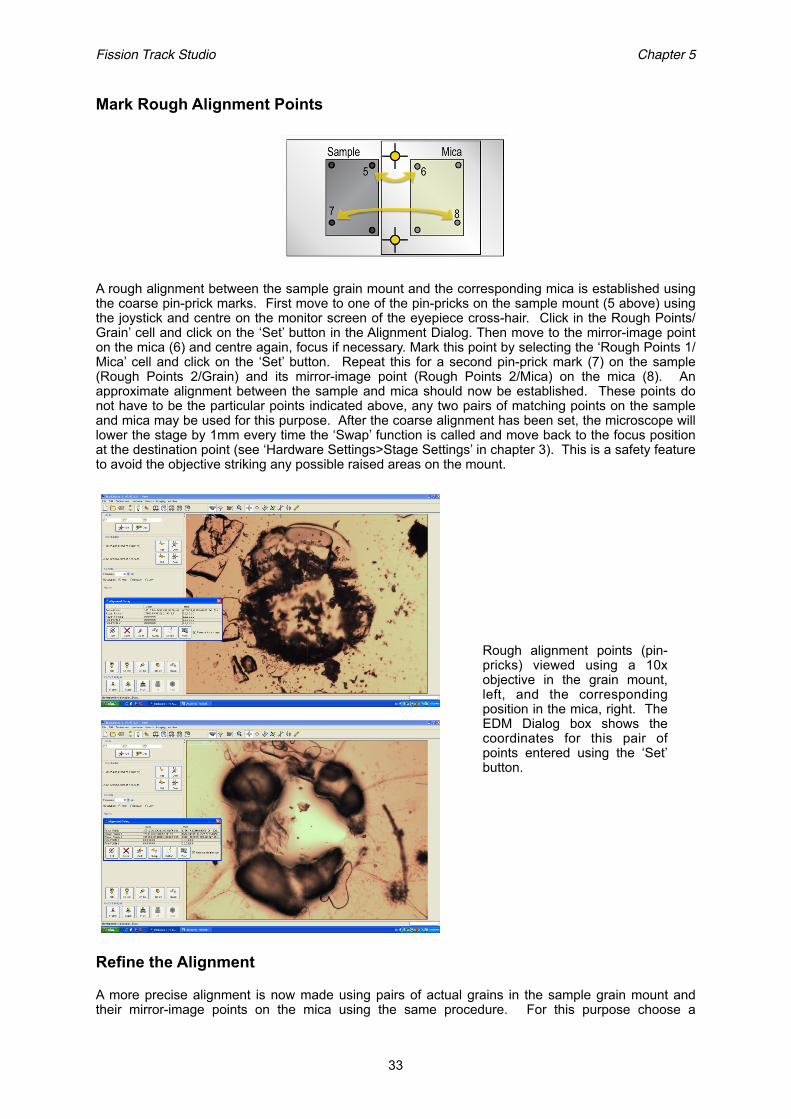
Mark Rough Alignment Points

A rough alignment between the sample grain mount and the corresponding mica is established using the coarse pin-prick marks. First move to one of the pin-pricks on the sample mount (5 above) using the joystick and centre on the monitor screen of the eyepiece cross-hair. Click in the Rough Points/Grain’ cell and click on the ‘Set’ button in the Alignment Dialog. Then move to the mirror-image point on the mica (6) and centre again, focus if necessary. Mark this point by selecting the ‘Rough Points 1/Mica’ cell and click on the ‘Set’ button. Repeat this for a second pin-prick mark (7) on the sample (Rough Points 2/Grain) and its mirror-image point (Rough Points 2/Mica) on the mica (8). An approximate alignment between the sample and mica should now be established. These points do not have to be the particular points indicated above, any two pairs of matching points on the sample and mica may be used for this purpose. After the coarse alignment has been set, the microscope will lower the stage by 1mm every time the ‘Swap’ function is called and move back to the focus position at the destination point (see ‘Hardware Settings>Stage Settings’ in chapter 3). This is a safety feature to avoid the objective striking any possible raised areas on the mount.

Refine the Alignment

A more precise alignment is now made using pairs of actual grains in the sample grain mount and their mirror-image points on the mica using the same procedure. For this purpose choose a


33

Rough alignment points (pin-pricks) viewed using a 10x objective in the grain mount, left, and the corresponding position in the mica, right. The EDM Dialog box shows the coordinates for this pair of points entered using the ‘Set’ button.

distinctive, and preferably isolated, small grain in the sample mount, precisely centre it and mark its position by selecting the ‘Fine Points1/Grain’ cell and pressing the ‘Set’ button. This is usually performed at high magnification (50x or 100x) and you can also click out a polygon to show the grain outline using the ‘Outline’ tool to help see the equivalent area on the mica.

Once the first fine point is set, pressing the ‘Swap’ button will take you to the approximate location of the image of this grain on the mica, based on the coarse alignment. Any outline drawn on the grain will be mirror-imaged at the mica position to help. Refine the position of this point by centering it on the monitor screen (the mouse ‘click to centre’ function is usually the easiest way to do this, but the joystick may also be used) and refocussing with the microscope focus controls. Once properly centred, mark the position by selecting the appropriate cell in the EDM Dialog box and pressing ‘Set’.

Repeat this process for a second fine point on the sample and mica. A new fine alignment has now been established that replaces the earlier rough alignment. The alignment can be checked by marking any point on the sample grain mount with the ‘add grain’ function, and pressing ‘Swap’. Alternatively click in one of the cells and use the ‘Go To’ button to go to the position of any of the marked points. Additional pairs of fine points can be added to further improve the alignment. Any additional pairs of fine alignment points will add to the first fine alignment in a progressive average, but the initial rough alignment is deleted.


34

Fine alignment points (a small zircon crystal in an apatite mount) viewed using a 100x objective in the grain mount in reflected light, left, and the corresponding position in the mica in transmitted light, right. The EDM Dialog box shows the coordinates for this pair of fine points as entered using the ‘Set’ button. An outline of the grain has been drawn using the ‘outline’ tool around the grain image and transferred to the mica image to assist with the alignment. In this case the mica image has been reversed (mirror-imaged) so as to match the appearance in the grain mount. The option to reverse the mica image can be selected in the EDM Dialog box, which can be reopened at any time.

Using the EDM system

Once a satisfactory alignment is established, the Alignment Dialog can be closed. TrackWorks will now automatically generate coordinates for the mica position equivalent to every grain marked on the sample using the ‘Add’ button. The ‘Grain’ list will now include the equivalent ‘Mica’ points for each grain that has been marked. The ‘Swap’ button will move back and forth between these pairs as needed, from grain to mica or from mica to grain. In addition, double clicking on any grain or its mica equivalent in the grain list will automatically move the microscope to that position.

Fission tracks in the grain and mica can now be measured in one of three ways depending on the sample quality and the preferences of the operator. The tracks may be counted manually looking down the microscope, and tallying the track count in the conventional manner, by defining a Region of Interest using the ‘RoI’ tool and clicking individual tracks on screen using the count tracks tool, or by capturing complete image sets using the Capture image option ‘All’. Captured images are then counted automatically and reviewed in FastTracks.

In the EDM mode, the capture ‘All’ option in the ‘Capture Images’ panel will capture image sets at both grain and mica localities for each marked grain position in the batch and save these to disc. If the position of a point on the mica needs to be updated, then the updated position becomes the new mica position rather than the originally calculated position, so it is possible to refine individual mica positions in the same way as for grain positions. The grain and mica images are saved as they appear under the microscope, without reversal of the mica images. They can be reversed again in FastTracks if desired.

Generating Points for Standard Micas

TrackWorks includes a tool for generating a grid of uniformly spaced points across a sample with a large area of uniform track density, such as that in a mica external detector over a standard glass. It is assumed that the track density is uniform over the large area of the mica and that a regular grid will therefore provide a suitable sampling strategy. This tool is activated by pressing the grid generator icon in the tool bar. The following dialog box will appear.

The tool generates a uniform grid in a rectangular area defined by two corner points. SImply move to one corner of the desired area and press the ‘Set Corner 1’ button. Then move to the second (opposite) corner and press the ‘Set Corner 2’ button. Now indicate how many grid lines are desired across the width and height of this rectangular area using the selection boxes and press Generate Points. A 5 x 5 grid is generated in this example, i.e. 25 points. The generated points will automatically appear in the Grain List in the side bar. It is wise to quickly visit each point by double-clicking on it, refining the focus, and position if desired, and pressing update. You can also step through the sequence by pressing Control + Arrow keys on the keyboard. Simply delete or adjust any unsuitable points using the ‘Delete’ button below the grain list.


35


36

6. MEASURING TRACK DIMENSIONSIntroduction:

Fission Track Studio contains a number of tools to assist in the measurement of track dimensions and orientations. These tools are available in both TrackWorks, for measurements on live images, and in FastTracks for measurement on captured images. There are four tools that are used for this purpose each represented by a different icon on the tool bar. They are, the c-axis tool, the track length tool, the Dpar tool and the Dimension tool.

The c-axis Tool

This tool is used for measuring the azimuth c-axis direction in grains that have their c-axes lying in the horizontal plane of the polished surface. The tool only works satisfactorily for such grains. The orientation of the c-axis in the vertical plane may be judged from the appearance of polishing scratches on the surface and the degree to which the track etch pits are parallel to each other, as observed in reflected light. The c-axis tool is therefore best used in reflected light at high magnification and should only be used for grains that have a strong alignment of

their track etch pits under these conditions..

Each grain in a mount will have a different c-axis direction, so the c-axis tool can only be used when at least one grain has been marked. If no grain has been marked, then an error message saying ʻNo grain selectedʼ will appear. If no grain has yet been marked, click on ʻAddʼ in the Grains panel. If a number of grains have already been marked, then select the particular grain for which a measurement is required by clicking that grain in the grain list.

The tool is activated by clicking on the icon in the tool bar. Proceed by clicking at one point on the image and moving the pointer away from it. A line will be dragged out to the current position of the pointer, with a set of parallel lines on each side of it. Move the pointer so that the lines are parallel to the long axes of the track etch pits. The spacing between the parallel lines can be varied by moving the scroll wheel to make it easier to judge how parallel all of the features are. Once a satisfactory alignment has been established, click again at a second point well away from the first. The parallel lines will disappear leaving the centre line as a reference direction for the c-axis. The c-axis direction can be removed by right-clicking on the line and selecting ʻDelete c-axisʼ. It is also possible to pick up one of the ̒ handleʼ boxes at either end of the marked c-axis line, and realign it should this be necessary.

Fission Track Studio# Chapter 6

37

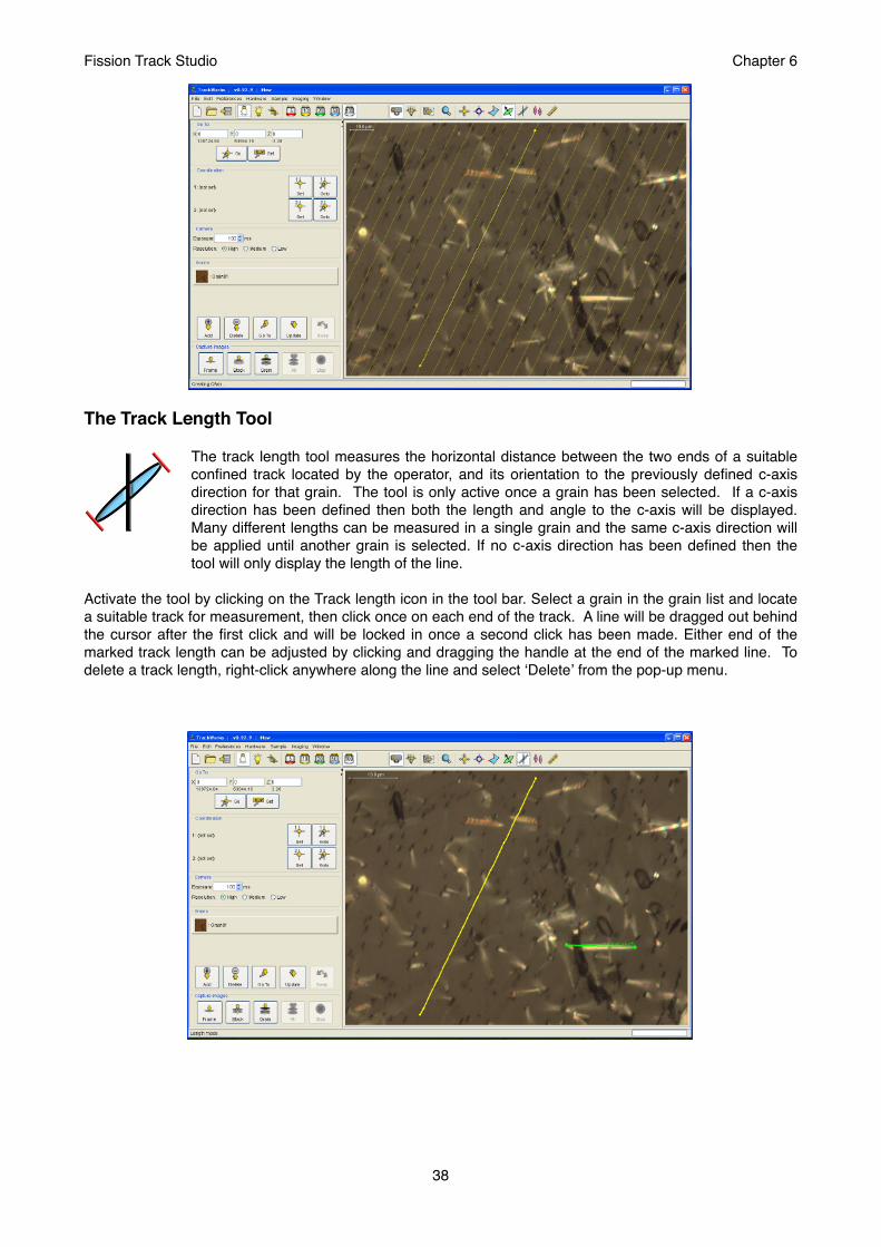
The Track Length Tool

The track length tool measures the horizontal distance between the two ends of a suitable confined track located by the operator, and its orientation to the previously defined c-axis direction for that grain. The tool is only active once a grain has been selected. If a c-axis direction has been defined then both the length and angle to the c-axis will be displayed. Many different lengths can be measured in a single grain and the same c-axis direction will be applied until another grain is selected. If no c-axis direction has been defined then the tool will only display the length of the line.

Activate the tool by clicking on the Track length icon in the tool bar. Select a grain in the grain list and locate a suitable track for measurement, then click once on each end of the track. A line will be dragged out behind the cursor after the first click and will be locked in once a second click has been made. Either end of the marked track length can be adjusted by clicking and dragging the handle at the end of the marked line. To delete a track length, right-click anywhere along the line and select ʻDeleteʼ from the pop-up menu.


38

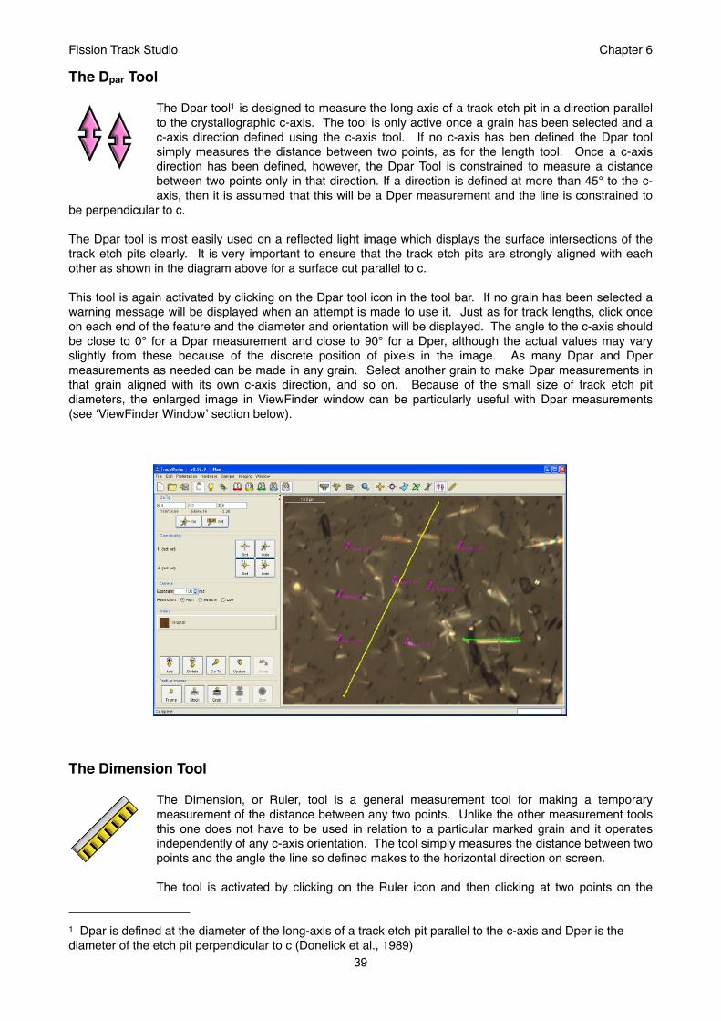
The Dpar Tool

The Dpar tool1 is designed to measure the long axis of a track etch pit in a direction parallel to the crystallographic c-axis. The tool is only active once a grain has been selected and a c-axis direction defined using the c-axis tool. If no c-axis has ben defined the Dpar tool simply measures the distance between two points, as for the length tool. Once a c-axis direction has been defined, however, the Dpar Tool is constrained to measure a distance between two points only in that direction. If a direction is defined at more than 45° to the c-axis, then it is assumed that this will be a Dper measurement and the line is constrained to

be perpendicular to c.

The Dpar tool is most easily used on a reflected light image which displays the surface intersections of the track etch pits clearly. It is very important to ensure that the track etch pits are strongly aligned with each other as shown in the diagram above for a surface cut parallel to c.

This tool is again activated by clicking on the Dpar tool icon in the tool bar. If no grain has been selected a warning message will be displayed when an attempt is made to use it. Just as for track lengths, click once on each end of the feature and the diameter and orientation will be displayed. The angle to the c-axis should be close to 0° for a Dpar measurement and close to 90° for a Dper, although the actual values may vary slightly from these because of the discrete position of pixels in the image. As many Dpar and Dper measurements as needed can be made in any grain. Select another grain to make Dpar measurements in that grain aligned with its own c-axis direction, and so on. Because of the small size of track etch pit diameters, the enlarged image in ViewFinder window can be particularly useful with Dpar measurements (see ʻViewFinder Windowʼ section below).

The Dimension Tool

The Dimension, or Ruler, tool is a general measurement tool for making a temporary measurement of the distance between any two points. Unlike the other measurement tools this one does not have to be used in relation to a particular marked grain and it operates independently of any c-axis orientation. The tool simply measures the distance between two points and the angle the line so defined makes to the horizontal direction on screen.

The tool is activated by clicking on the Ruler icon and then clicking at two points on the


39

1 Dpar is defined at the diameter of the long-axis of a track etch pit parallel to the c-axis and Dper is the diameter of the etch pit perpendicular to c (Donelick et al., 1989)

screen. A line is displayed between these points with its length and angle to the horizontal labelled beside it. Only one such dimension is active at any one time and the dimension so measured is not stored or tabulated for export. As before, the line is deleted by right clicking on it and selecting ʻDeleteʼ in the pop-up menu. An existing line must be deleted before another measurement can be made.

Region of Interest

The area within which tracks are counted may be restricted to a particular ʻRegion of Interestʼ (RoI) within a field of view. The tool is activated by selecting the Region of Interest icon in the tool bar and will only work after a particular grain has been selected. After a RoI has been created it is revealed only when that particular grain is selected and is relevant only at the magnification for which it was defined.

There are several modes of use associated with this tool, the simplest being merely to click out a polygon on the screen. A polygon can be of any shape and may even cross back on itself, with only tracks within the RoI being counted. The area of the RoI is calculated to be just the area, or areas, that is enclosed within the polygon. The polygon is closed either by double clicking at any point, or by clicking again on the first point defined.

If no region of Interest is already marked, then simply dragging the cursor will define a rectangular RoI on the screen between the start and end points. Also a default region of interest can be defined by right-clicking on the screen and selecting ʻDefault ROIʼ from the pop-up menu. The Default RoI is a rectangle inset a short distance from the edge of the image field, with the degree of inset being defined in pixels in the ʻOverlay Optionsʼ item under the ʻPreferencesʼ menu.

A region of interest can easily be adjusted after it is defined by simply clicking and dragging on the handles marking the vertices or on any of the lines. Additional points can be added by right-clicking on a line and selecting ʻAdd point in this segmentʼ in the pop-up menu. The right-click menu also contains options to ʻDelete All Points” and to mark the ʻDefault ROIʼ.

Manually Counting Tracks

Tracks may be counted manually onscreen by selecting the ʻManually Edit Tracksʼ tool on the menu bar. This tool has two functions, the one described here is to manually mark counted tracks on screen in TrackWorks, and the other is to edit the results of automatic counting in FastTracks. When this tool is active, the mouse cursor becomes a red cross over the main image window (the colour many be changed). Clicking on a track leaves a small ʻxʼ mark on the screen and tracks to be counted are selected by clicking on each one in turn. Right clicking on a point produces a pop-up menu with a number of options for

multiple tracks at a certain point, as may be found with overlapping tracks. A track can be deleted from the count by moving the cursor over its cross mark and clicking on it. The marked cross will disappear and the count will be reduced by one. It can also be deleted by selectingʼ0ʼ in the right-click menu.


40

A grid of user selectable size can be overlaid on the screen to facilitate scanning the field of view, by selecting this option under ʻOverlay Optionsʼ item under the ʻPreferencesʼ menu. If a Region of Interest has been defined, only those tracks within the RoI will be counted. The program constantly keeps track of the number of tracks and the area being counted and the count data can be viewed in Count Summary item under the Sample Menu.

Overlay Options

All of these data measurements are displayed as individual layers in the Overlay layer, which is shown superimposed on the live or stored screen image. These include both manual track counts and c-axis, track length and Dpar measurements. A cross hair and scale bar can also be made visible int eh Overlay. All of these layers may be selected din the Overlay Options window under the Preferences menu.

Images vary significantly in colour and brightness, so that some colours in the overlay may not be clearly visible. It may be necessary to change the colour scheme to enhance Overlay visibility on screen. The colours assigned to various features in the Overlay, such as the RoI, may be changed simply in the ʻColor Optionsʼ pane of the Overlay Options Dialog box. Simply select the ʻColor Optionsʼ Tab in the ʻOverlay Optionsʼ Dialog under the ʻPreferencesʼ Menu, and click on the colour of any of the features in the list. A colour palette will appear in which a new colour can be chosen to replace the previous colour.

The third tab of the Overlay Options Dialog presents a series of different Cursors that can be selected for use when making measurements on tracks in the Overlay. Both the shape and colour of the cursor may be selected in order to enhance the visibility of the cursor against the background in a particular sample and also to enable the maximum visibility of the object underneath the cursor.


41

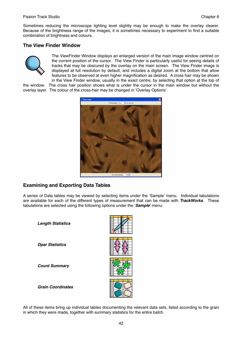
Sometimes reducing the microscope lighting level slightly may be enough to make the overlay clearer. Because of the brightness range of the images, it is sometimes necessary to experiment to find a suitable combination of brightness and colours.

The View Finder Window

The ViewFinder Window displays an enlarged version of the main image window centred on the current position of the cursor. The View Finder is particularly useful for seeing details of tracks that may be obscured by the overlay on the main screen. The View Finder image is displayed at full resolution by default, and includes a digital zoom at the bottom that allow features to be observed at even higher magnification as desired. A cross hair may be shown in the View Finder window, usually in the exact centre, by selecting that option at the top of

the window. The cross hair position shows what is under the cursor in the main window but without the overlay layer. The colour of the cross-hair may be changed in ʻOverlay Optionsʼ.

Examining and Exporting Data Tables

A series of Data tables may be viewed by selecting items under the ʻSampleʼ menu. Individual tabulations are available for each of the different types of measurement that can be made with TrackWorks. These tabulations are selected using the following options under the ʻSampleʼ menu:

! Length Statistics

! Dpar Statistics

! Count Summary

! Grain Coordinates

All of these items bring up individual tables documenting the relevant data sets, listed according to the grain in which they were made, together with summary statistics for the entire batch.


42

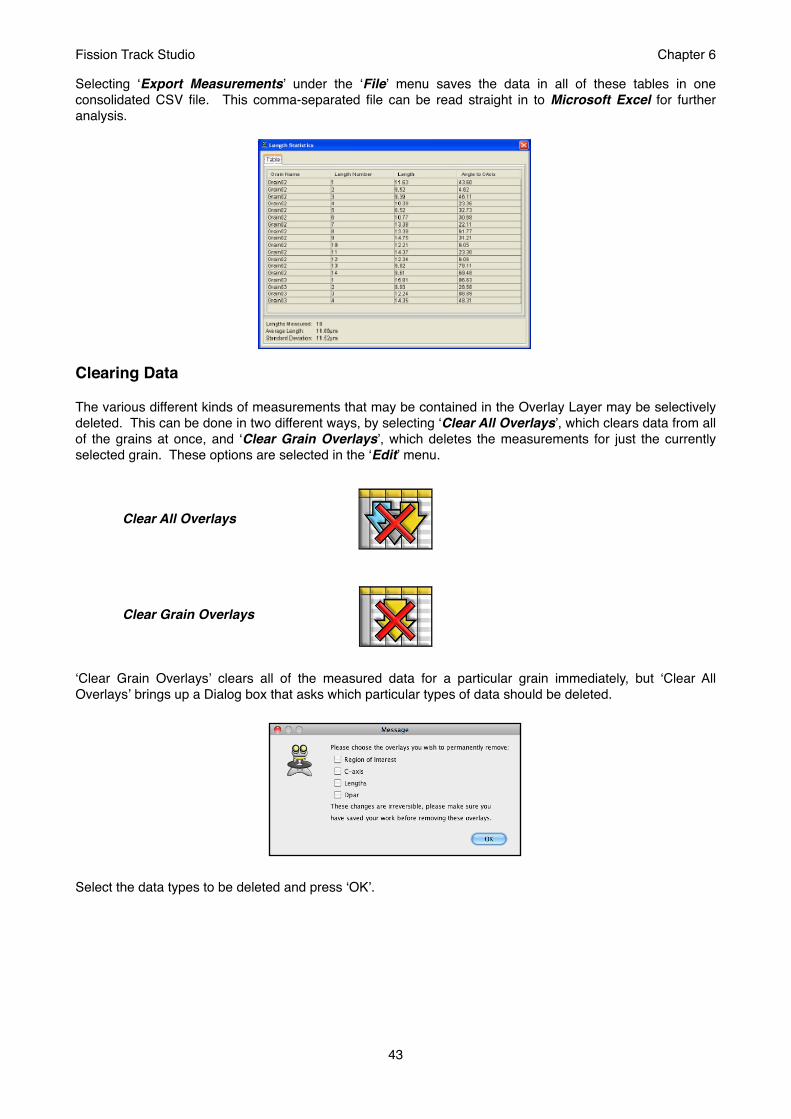
Selecting ʻExport Measurementsʼ under the ʻFileʼ menu saves the data in all of these tables in one consolidated CSV file. This comma-separated file can be read straight in to Microsoft Excel for further analysis.

Clearing Data

The various different kinds of measurements that may be contained in the Overlay Layer may be selectively deleted. This can be done in two different ways, by selecting ̒ Clear All Overlaysʼ, which clears data from all of the grains at once, and ʻClear Grain Overlaysʼ, which deletes the measurements for just the currently selected grain. These options are selected in the ʻEditʼ menu.

# Clear All Overlays

# Clear Grain Overlays

ʻClear Grain Overlaysʼ clears all of the measured data for a particular grain immediately, but ʻClear All Overlaysʼ brings up a Dialog box that asks which particular types of data should be deleted.

Select the data types to be deleted and press ʻOKʼ.


43


44

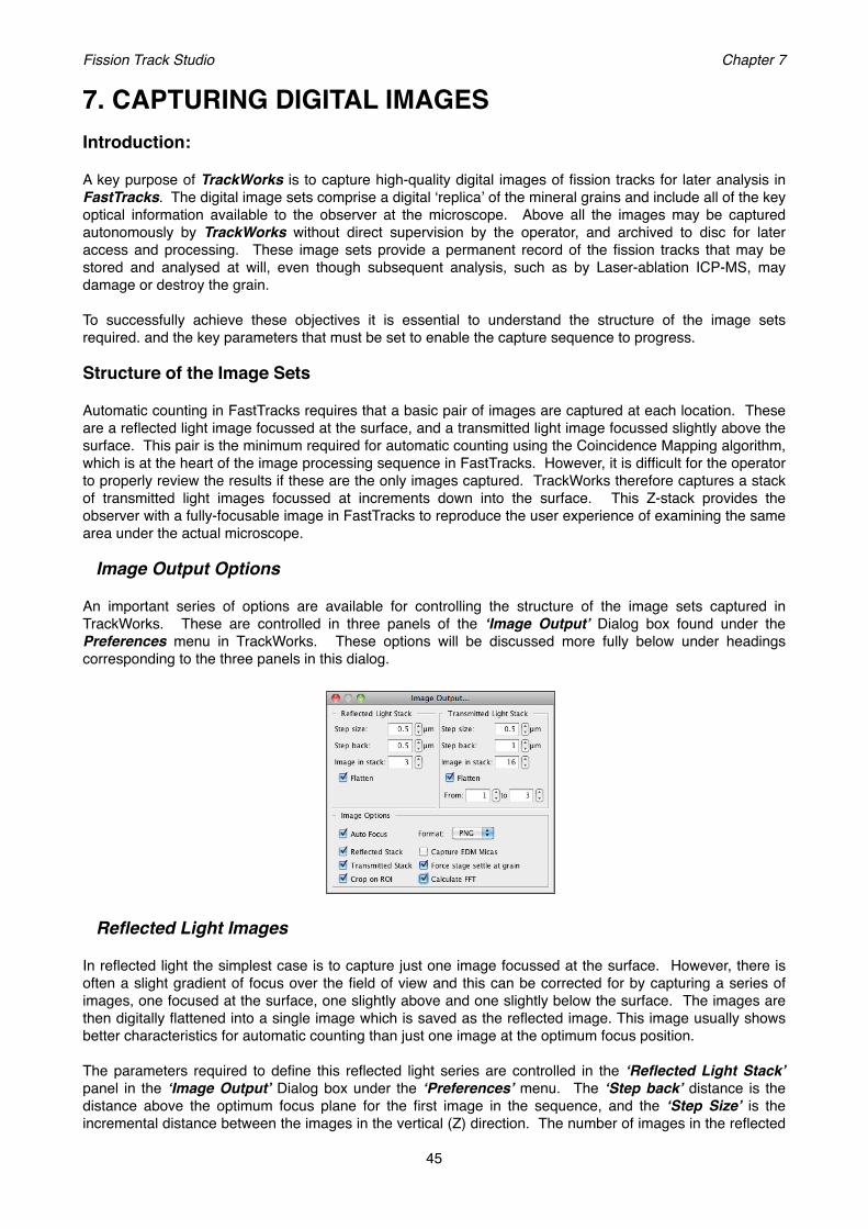
7. CAPTURING DIGITAL IMAGESIntroduction:

A key purpose of TrackWorks is to capture high-quality digital images of fission tracks for later analysis in FastTracks. The digital image sets comprise a digital ʻreplicaʼ of the mineral grains and include all of the key optical information available to the observer at the microscope. Above all the images may be captured autonomously by TrackWorks without direct supervision by the operator, and archived to disc for later access and processing. These image sets provide a permanent record of the fission tracks that may be stored and analysed at will, even though subsequent analysis, such as by Laser-ablation ICP-MS, may damage or destroy the grain.

To successfully achieve these objectives it is essential to understand the structure of the image sets required. and the key parameters that must be set to enable the capture sequence to progress.

Structure of the Image Sets

Automatic counting in FastTracks requires that a basic pair of images are captured at each location. These are a reflected light image focussed at the surface, and a transmitted light image focussed slightly above the surface. This pair is the minimum required for automatic counting using the Coincidence Mapping algorithm, which is at the heart of the image processing sequence in FastTracks. However, it is difficult for the operator to properly review the results if these are the only images captured. TrackWorks therefore captures a stack of transmitted light images focussed at increments down into the surface. This Z-stack provides the observer with a fully-focusable image in FastTracks to reproduce the user experience of examining the same area under the actual microscope.

Image Output Options

An important series of options are available for controlling the structure of the image sets captured in TrackWorks. These are controlled in three panels of the ʻImage Outputʼ Dialog box found under the Preferences menu in TrackWorks. These options will be discussed more fully below under headings corresponding to the three panels in this dialog.

Reflected Light Images

In reflected light the simplest case is to capture just one image focussed at the surface. However, there is often a slight gradient of focus over the field of view and this can be corrected for by capturing a series of images, one focused at the surface, one slightly above and one slightly below the surface. The images are then digitally flattened into a single image which is saved as the reflected image. This image usually shows better characteristics for automatic counting than just one image at the optimum focus position.

The parameters required to define this reflected light series are controlled in the ʻReflected Light Stackʼ panel in the ʻImage Outputʼ Dialog box under the ʻPreferencesʼ menu. The ʻStep backʼ distance is the distance above the optimum focus plane for the first image in the sequence, and the ʻStep Sizeʼ is the incremental distance between the images in the vertical (Z) direction. The number of images in the reflected


45

light sequence is selected in theʻImages in Stackʼ option. Three is normally the default number selected, but it is also possible to capture more images in this sequence if required. If the focus is satisfactory over the whole field of view than it is possible to simply capture a single reflected light image. Simply reduce the number of ʻImages in Stackʼ to one, change ʻStep sizeʼ and ʻStep backʼ to zero, and deselect the ʻFlattenʼ option.

Transmitted Light Images

For the transmitted light sequence, the parameters to be set are found in the ʻTransmitted Light Stackʼ panel at the top right of the ʻImage Outputʼ Dialog. These parameters are similar to those for reflected light. As before, the ʻStep Sizeʼ determines the vertical distance between successive image planes and the ʻImages in Stackʼ determines the total number of images to be captured. The capture sequence begins at the optimal focus position and then defocuses a small distance above the surface to capture the Step back image.

For the transmitted light stack the number of images in the stack will be much larger, so that the operator can focus down through the region where most of the tracks are. Fifteen images in the stack at a spacing of 0.5 µm will provide a sufficient sense of smooth and continuous focusing to a depth of 7.5µm below the surface. This contains the depth information for the great majority of tracks and it is the near-surface component of this sequence that is most useful in enabling the operator to discriminate tracks and to resolve overlaps. The minimum useful step size is about 0.3 µm and there is no useful depth resolution to be gained by going to an even smaller step size. More images can also be captured in the stack if desired, but at the significant penalty of a substantial increase in the already very large file size, which can have a deleterious effect on performance.

The distance above the surface for the Step back image is a key parameter in the success of the Coincidence mapping process and should normally be set by an amount in the range 0.5 to 1.0 µm. The aim is to produce a slightly defocused image of the tracks which has no bright spots in the centre of the tracks, as shown below for fission tracks in mica.

It is also possible to produce a flattened image derived from the upper few images in the sequence, which will be used as the step back image. This may be useful when there is a focus gradient across the field of view, and is captured in an analogous way to the reflected light sequence. This option is activated by selecting ʻFlattenʼ in the ʻTransmitted Light Stackʼ panel in the ʻImage Outputʼ dialog and then selecting the range of images in the overall stack to be flattened to make this image. Three images starting with the stepback image (images 1-3) is usually sufficient, but it is worth experimenting with the results of flattening


46

more than this and perhaps increasing the stepback distance to get the best output. Unlike the case with the reflected light stack the flattened transmitted light image is saved independently of the images in the main stack, so that all of the focus information remains available.

Autofocus Settings

The key reference plane for the image sequence captured at each location is the etched surface, all other image planes being captured at controlled intervals above and below this surface. TrackWorks therefore contains an autofocus routine that will find the optimum focus surface as the first step to capturing images at each location. The autofocus routine works by searching for the plane with the maximum image contrast, and therefore will only work where there are features in the field of view, such as fission tracks, and polishing scratches, that relate to the surface. The routine is likely to fail to find a focus position if the field is entirely blank, as may happen, for example on a mica surface with no fission tracks visible.

To activate this option select ʻAutofocusʼ in the ʻImage Optionsʼ panel of the ʻImage Outputʼ dialog. The parameters controlling the autofocus routine are set in the ̒ Autofocus Settingsʼ dialog box found under the ʻPreferencesʼ menu. The autofocus routine progresses by defocussing by a predetermined distance above the expected focus position and moving in coarse increments to a similar distance below it. By default the focus range is set to 10 µm and the ʻCoarse stepʼ size is set to 1 µm. Once this sequence is completed the region near the best focus position is explored again at a fine step size (0.3 µm by default) to ascertain the optimum focus position. The maximum brightness for this search may also be set here and is set at a grey scale value of 255 by default, so that this covers the entire possible range from black to white. Normally this does not need adjustment.


47

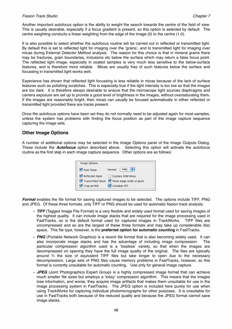
Another important autofocus option is the ability to weight the search towards the centre of the field of view. This is usually desirable, especially if a focus gradient is present, so this option is selected by default. The centre weighting conducts a linear weighting from the edge of the image (0) to the centre (1.0).

It is also possible to select whether the autofocus routine will be carried out in reflected or transmitted light. By default this is set to reflected light for imaging over the ʻgrainsʼ, and to transmitted light for imaging over micas during External Detector Method analysis. The reason for this choice is that in mineral grains there may be fractures, grain boundaries, inclusions etc below the surface which may return a false focus point. The reflected light image, especially in coated samples is very much less sensitive to the below-surface features, and is therefore more reliable. Micas are usually free of such features below the surface and focussing in transmitted light works well.

Experience has shown that reflected light focussing is less reliable in micas because of the lack of surface features such as polishing scratches. This is especially true if the light intensity is too low so that the images are too dark. It is therefore always desirable to ensure that the microscope light sources diaphragms and camera exposure are set up to provide a good level of brightness in the images, without oversaturating them. If the images are reasonably bright, then micas can usually be focused automatically in either reflected or transmitted light provided there are tracks present.

Once the autofocus options have been set they do not normally need to be adjusted again for most samples, unless the system has problems with finding the focus position as part of the image capture sequence capturing the image sets.

Other Image Options

A number of additional options may be selected in the Image Options panel of the Image Outputs Dialog. These include the Autofocus option described above. Selecting this option will activate the autofocus routine as the first step in each image capture sequence. Other options are as follows:

Format enables the file format for saving captured images to be selected. The options include TIFF, PNG and JPEG. Of these three formats, only TIFF or PNG should be used for automatic fission track analysis.

• TIFF (Tagged Image File Format) is a very flexible and widely used format used for saving images of the highest quality. It can include image stacks that are required for the image processing used in FastTracks, so is the default format used for captured images in TrackWorks. TIFF files are uncompressed and so are the largest of these three formats and may take up considerable disc space. This file type, however, is the preferred option for automatic counting in FastTracks.

• PNG (Portable Network Graphics) is a recent file format that is also becoming widely used. It can also incorporate image stacks and has the advantage of including image compression. The particular compression algorithm used is a ʻlosslessʼ variety, so that when the images are decompressed on opening they have the full image quality of the original. The files are typically around ⅓ the size of equivalent TIFF files but take longer to open due to the necessary decompression. Large sets of PNG files cause memory problems in FastTracks, however, so this format is currently unsuitable for automatic counting. Use only for general image capture.

• JPEG (Joint Photographics Expert Group) is a highly compressed image format that can achieve much smaller file sizes but employs a ʻlossyʼ compression algorithm. This means that the images lose information, and worse, they acquire image artifacts that makes them unsuitable for use in the image processing system in FastTracks. The JPEG option is included here purely for use when using TrackWorks for capturing individual photomicrographs for other purposes. It is unsuitable for use in FastTracks both because of the reduced quality and because the JPEG format cannot save image stacks.


48

Reflected Stack - select this option to capture a z-stack in reflected light, using the parameters selected in the Reflected Light Stack panel. At present this option simply leads to a single flattened image from the reflected stack.

Transmitted Stack - select this option to capture a z-stack in transmitted light, using the parameters selected in the Transmitted Light Stack panel. In this case the full stack is saved along with the step-back image and, if selected in the transmitted stack panel, a flattened version of the indicated number of images from the upper part of the stack.

Crop on RoI - when selected, this option crops the captured images before saving them to the smallest bounding rectangle that will enclose the Region of Interest, where this has been marked. Using this option is the best way of reducing image size to include just that part of the visible field that contains the target information. Use it to decrease the amount of extraneous clutter in the images, such as grain boundaries or major defects, and also to minimize the size of the images, so as to improve processing performance.

Capture EDM Micas - when using the External Detector method, select this option to capture paired image sets on the grain mount and the mica external detector. The same sequence of images indicated in the Transmitted and Reflected Light Stack Panels in Image Outputs will be applied to both the marked grains and their paired mica equivalents.

Force Stage Settle at Grain - this option should normally be selected so that any residual backlash in the stage position (or possibly movement of the reflector cube) is removed before image capture begins. Forcing stage settle works by rapidly switching the light shutters on the microscope before image capture begins. The resulting small vibration of the microscope relieves any residual backlash, so that subsequent shutter operations do not produce any further movement. The option is necessary because movement of the reflected and transmitted shutters when changing illumination modes can induce a slight movement of the stage because of this backlash. Such movements are small, usually only 1-2 µm, but can lead to a systematic misalignment of the reflected and transmitted images, so that the coincidence mapping algorithm in FastTracks does not work properly. There is a tool for correcting any remaining mismatch in the images in FastTracks should this be necessary.

Calculate FFT - one of the important steps in the image processing sequence is a correction for variations in the background intensity across each image. This procedure uses a Fast Fourier Transform Bandpass Filter (ʻFFTʼ). Selecting this option in the Image Output panel of TrackWorks will apply the FFT filter to all of the images before they are saved to disc. This is usually selected because the FFT filter is the single most time-consuming step in the image processing sequence. By selecting this option here in TrackWorks, this slow step is completed during autonomous image capture sequence, making subsequent processing in FastTracks much faster. If this option is not selected in TrackWorks, the FFT filter will still be applied during processing in FastTracks.

Final Adjustment before image capture

Once a series of grains have been chosen, and if appropriate, an EDM alignment completed, it is good practice to quickly check all of the marked locations for any final adjustment in position or focus. This is most simply done by double-clicking on each in turn in the grain list, or selecting a grain or mica and either clicking the Go To button, or selecting Go To in the right-click pop-up menu. For any grain or mica you can always click ʻSwapʼ to jump to the paired equivalent point. Once at each location you can adjust the position using the click to centre option (best) or using the joystick and refocussing manually or with the mouse scroll wheel. Once you are satisfied with position and focus, press the Update button, or select Update in the right-click pop-up menu. Such adjustments should always be carried out using the 100x objective that will be used for image capture.

The final step before capturing images is to ensure that suitable default camera exposure values are set to appropriate values in both transmitted and reflected light using the objective to be used for image capture, almost always the 100x. The exposure levels are set using the ʻPreset Exposure Valuesʼ panel in the ʻObjective settingsʼ dialog under the ʻHardwareʼ menu, as described under ʻExposure Presetsʼ in Chapter 3, ʻSetting Up and Operating the Microscopeʼ.


49

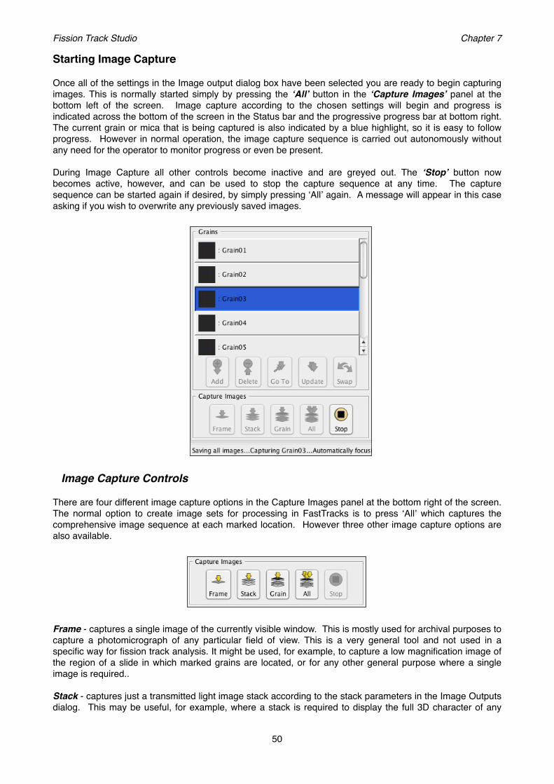
Starting Image Capture

Once all of the settings in the Image output dialog box have been selected you are ready to begin capturing images. This is normally started simply by pressing the ʻAllʼ button in the ʻCapture Imagesʼ panel at the bottom left of the screen. Image capture according to the chosen settings will begin and progress is indicated across the bottom of the screen in the Status bar and the progressive progress bar at bottom right. The current grain or mica that is being captured is also indicated by a blue highlight, so it is easy to follow progress. However in normal operation, the image capture sequence is carried out autonomously without any need for the operator to monitor progress or even be present.

During Image Capture all other controls become inactive and are greyed out. The ʻStopʼ button now becomes active, however, and can be used to stop the capture sequence at any time. The capture sequence can be started again if desired, by simply pressing ʻAllʼ again. A message will appear in this case asking if you wish to overwrite any previously saved images.

Image Capture Controls

There are four different image capture options in the Capture Images panel at the bottom right of the screen. The normal option to create image sets for processing in FastTracks is to press ʻAllʼ which captures the comprehensive image sequence at each marked location. However three other image capture options are also available.

Frame - captures a single image of the currently visible window. This is mostly used for archival purposes to capture a photomicrograph of any particular field of view. This is a very general tool and not used in a specific way for fission track analysis. It might be used, for example, to capture a low magnification image of the region of a slide in which marked grains are located, or for any other general purpose where a single image is required..

Stack - captures just a transmitted light image stack according to the stack parameters in the Image Outputs dialog. This may be useful, for example, where a stack is required to display the full 3D character of any


50

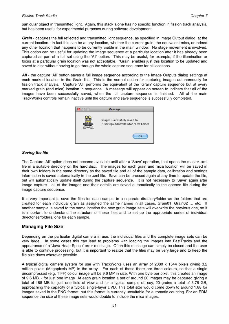
particular object in transmitted light. Again, this stack alone has no specific function in fission track analysis, but has been useful for experimental purposes during software development.

Grain - captures the full reflected and transmitted light sequence, as specified in Image Output dialog, at the current location. In fact this can be at any location, whether the current grain, the equivalent mica, or indeed any other location that happens to be currently visible in the main window. No stage movement is involved. This option can be useful for updating the image sequence at a particular location after it has already been captured as part of a full set using the ʻAllʼ option. This may be useful, for example, if the illumination or focus at a particular grain location was not acceptable. ʻGrainʼ enables just this location to be updated and saved to disc without having to go through the whole capture sequence for all locations.

All - the capture ʻAllʼ button saves a full image sequence according to the Image Outputs dialog settings at each marked location in the Grain list. This is the normal option for capturing images autonomously for fission track analysis. Capture ʻAllʼ performs the equivalent of the ʻGrainʼ capture sequence but at every marked grain (and mica) location in sequence. A message will appear on screen to indicate that all of the images have been successfully saved, when the full capture sequence is finished. All of the main TrackWorks controls remain inactive until the capture and save sequence is successfully completed.

Saving the file

The Capture ʻAllʼ option does not become available until after a ʻSaveʼ operation, that opens the master .xml file in a suitable directory on the hard disc. The images for each grain and mica location will be saved in their own folders in the same directory as the saved file and all of the sample data, calibration and settings information is saved automatically in the .xml file. Save can be pressed again at any time to update the file, but will automatically update itself during the capture sequence. It is not necessary to ʻSaveʼ again after image capture - all of the images and their details are saved automatically to the opened file during the image capture sequence.

It is very important to save the files for each sample in a separate directory/folder as the folders that are created for each individual grain as assigned the same names in all cases, Grain01, Grain02 … etc. If another sample is saved to the same location the new grain image sets will overwrite the previous one, so it is important to understand the structure of these files and to set up the appropriate series of individual directories/folders, one for each sample.

Managing File Size

Depending on the particular digital camera in use, the individual files and the complete image sets can be very large. In some cases this can lead to problems with loading the images into FastTracks and the appearance of a ʻJava Heap Spaceʼ error message. Often this message can simply be closed and the user is able to continue processing, but it is important to realize that the files may be very large and to keep the file size down wherever possible.

A typical digital camera system for use with TrackWorks uses an array of 2080 x 1544 pixels giving 3.2 million pixels (Megapixels MP) in the array. For each of these there are three colours, so that a single uncompressed (e.g. TIFF) colour image will be 9.6 MP in size. With one byte per pixel, this creates an image of 9.6 MB. - for just one image At each grain location a set of around 20 images may be captured giving a total of 188 MB for just one field of view and for a typical sample of, say, 20 grains a total of 3.76 GB, approaching the capacity of a typical single-layer DVD. This total size would come down to around 1.88 for images saved in the PNG format, but this format is currently unsuitable for automatic counting. For an EDM sequence the size of these image sets would double to include the mica images.


51

So it is clear that very large image sets may be created with TrackWorks. This is no longer a significant issue from the point of view of file storage, with very large capacity (1TB or more) hard disc drives, now available very cheaply, but it is not surprising that handling these large image files can cause problems in the software.

FastTracks only uses two images for each location in the automatic fission track counting system, which are processed rapidly and efficiently. Problems with large images usually come from handling large full resolution image stacks. FastTracks employs an efficient file loading method that only loads the image stacks for the currently selected grain.

There are a number of ways of managing the image size in TrackWorks:

• Limit the number of individual images in the image stacks. A total of 15 images at 0.5 µm spacing is more than enough to give the observer the experience of focussing on real tracks under the microscope. Remember that the image stacks are included only for this purpose, and are not required for automatic counting. The most important information in the stacks for identifying and discriminating tracks is actually near the surface, so it is possible to significantly reduce the number of images in the stacks, to perhaps only 8-10, with very little impact on the user experience. This will have a major effect, however, on reducing the overall file size and improving performance.

• Crop Images to a selected Region of Interest. Setting a Region of Interest in TrackWorks for each grain location, and selecting ʻCrop to RoIʼ in the Image Output dialog, dramatically reduces file size and generally leads to greatest improvement in performance. For example, selecting a RoI that has half the total image dimensions will reduce file size to one quarter of the full size image. These rectangular cropped images can also have any image proportions, so that they are very useful for selecting just the best area of a field of view for capture. The RoI selection is very flexible as each grain can have different proportions.

• Capture Images at Medium Resolution. This has a similar benefit to Cropping the images by reducing the number of pixels captured. Reducing the image resolution to medium works by capturing every second pixel from the camera array and therefore reduces file size to one quarter. Some recalibration will be required to use medium resolution images, however, and it is important to establish the appropriate settings in ʻObjective Settingsʼ dialog. Similarly, adjustments will be required in FastTracks to some of the image processing parameters, such as to the minimum and maximum track area in the Image Details dialog.

• (Save images in the PNG format). It is planned to introduce this option to reduce file size in a future version of the software. At the present time this option an be used to save images, but is not supported for automatic counting in FastTracks. The PNG format significantly reduces overall file size for storage, but does not actually improve performance in image handling. In fact it reduces overall performance slightly by introducing the additional step of decompression of the images when they are opened.


52

8. AUTOMATIC TRACK COUNTING IN FASTTRACKSIntroduction:

FastTracks enables the operator to view captured image sets made using TrackWorks, to run the automated counting routines, and to inspect the results. FastTracks operates as a virtual microscope enabling the captured imagery to be viewed in a manner similar to a real microscope. The captured z-stack can be scrolled to give a focusable image, observation can be switched between transmitted and reflected light, or these two modes can be overlaid using different degrees of transparency. The same track measurement tools available in TrackWorks are also present for use in FastTracks, the only difference being that in FastTracks these work on stored images rather than on the live image as in TrackWorks. In FastTracks the measurements remain stable with respect to the images, because there is no possibility of movement in the microscope. The use of these tools is described in Chapter 6 and is not repeated here.

Loading images

When FastTracks is first started, most of the tools in the Tool Bar are grayed out, leaving only the ʻNewʼ and ʻOpenʼ icons active. The first step in using FastTracks is to load an image set into the program using ʻOpenʼ under the File menu, or the equivalent icon in the Tool bar. Use the resulting ʻLoad Fileʼ Dialog box to navigate to the desired image set, select the .XML file for that set, and press ʻOpenʼ. The image set will then begin to load into FastTracks. This will load a series of thumbnail images, one for each grain, into the ʻNavigationʼ List on the left hand side bar. The currently active grain (the first grain in an unprocessed set) will also appear in the main widow. The images in the main ʻImage Viewʼ window are automatically scaled to fit to the window.

The image files generated by TrackWorks are very large, so FastTracks operates by loading the full image set for only one grain at a time. Once the images are loaded, the tool bar icons as well as the thumbnail images and the Focus Slider at the bottom of the main Image View window, will again become active. This will normally only take a few seconds, and the progress of loading the images can be monitored in the Status Bar and Progress Bar at the bottom of the main window (see Chapter 1). Importantly, the image set visible in the main Image View window will only be operational once the Focus Slider across the bottom has

become active. Once fully loaded the image can be focussed over the range of the captured z-stack using the mouse scroll-wheel, or by dragging on the Focus Slider across the bottom of the image window.

Move to any other grain by clicking on its thumbnail image in the ʻNavigationʼ List. While the new grain is loading the various tools will again be grayed out and the new grain set will only become active when the focus slider has returned to its normal active state. Remember that the images for each particular grain are only loaded into memory when that grain is selected, so this process takes almost the same time every time a new grain is selected. It is best not to attempt to carry out any other action until the new grain is fully loaded. This should only take a few seconds, so be patient!

When an EDM file is opened the Navigation Bar works somewhat differently to the paired sets of grain and mica thumbnails seen in TrackWorks. In FastTracks only a single set of thumbnail images appears at one time in the Navigation bar, either the grain images, or the mica images. Two radio buttons appear in theTool bar at the top of the main image window one for grains and one for micas. Selecting one of these options determines which set are displayed in the Navigation bar.

A file can be closed by selecting ʻCloseʼ under the File menu. Opening a new file will also automatically close the currently open file, so it is not necessary to explicitly close an open file in order to start work on a new one.


53

Viewing images

Once an image set for a particular grain, or its mica pair, has been loaded it is possible to switch between the focusable transmitted light stack and the reflected light image at will, as could be done under a real microscope. The transmitted light stack is focused either by using the mouse scroll wheel, but also by sliding the ʻFocusʼ slider across the bottom of the main window under the image. However, a variety of additional display settings are possible and these are selected using the ʻOptionsʼ panel at top right of the main window. These include the ability to overlay an adjustable grid on the image, to display a scale bar, to preview the area of a particular counted feature, and to show an overlay layer that will include the image analysis results once this has been performed. The transparency of the overlay, the reflected light image and the transmitted light image can also be adjusted, so that it is possible to view a partially transparent reflected light layer over the transmitted light image, for example. The transparency of these layers is adjusted by moving the slider bars in the ̒ Optionsʼ panel. The small arrow buttons on the left of the Options Dialog will close and open the right hand side panels to make more room for the main image window, if this is needed. Other options about which features are to be displayed in the overlay, are discussed below under ʻOverlay Optionsʼ.

Combining and switching between image states is carried out in the ʻToggle Imagesʼ mode which is the default state when a set of images are first opened. This mode can be selected at any time by clicking on the ʻToggle Imagesʼ icon in the tool bar. When in this mode a left-click in the main image window will toggle the overlay layer on and off, and a right-click will similarly toggle the reflected light image. This is generally more convenient and faster than selecting these options in the Options panel. These three layers are always

displayed in the order in which they appear in the ʻOptionsʼ panel, ie the transmitted light z-stack layer at the bottom, followed by the reflected light layer above, and the image analysis overlay on top.

The transmitted and reflected light images are displayed in full colour to best simulate their appearance under the microscope. In the overlay, the colours of all of the individual components in the image analysis and measurement layers are user-selectable in the ʻOverlay Optionsʼ dialog under the Settings menu (see below). The number of squares in the rectangular grid may be selected next to ̒ Gridʼ in the ʻʼOptions Panelʼ and the colour of the grid lines may also be selected to maximise contrast against the background image by clicking on the small colour box next to the grid square number. The grid colour may also be changed in the Overlay Options dialog.

An enlarged view of the section of the main window centred on the current cursor position

may be seen in the VIewFinder widow. This window operates in the same way as the same feature in TrackWorks as described in Chapter

6. Click on the ViewFinder icon in the tool bar to show the ViewFinder window. The magnification shown in this window can be set in the range 50-300% using the spinner box at the bottom of the window. A cross hair, in a user-selectable colour, can also be shown in the ViewFinder. As the cursor is moved around the main window the image moves in the ViewFinder so that the cross hair remains centred on the current cursor position in the main window, except where the cursor is near the edge, in which case the cross hairs themselves will move. The ViewFinder is useful when reviewing the results of automatic counting as it enables an enlarged view of features to be examined that may be obscured by the overlay in the main window.


54

Viewing microscope settings

The various settings used by TrackWorks when acquiring a particular image series may be shown under ʻOutput Infoʼ, and ʻView Hardwareʼ under the Settings Menu. Similarly the sample description details may be examined under ʻSample>Sample Infoʼ, or by clicking on the ʻSampleʼ tab in the Settings Dialog. This information is saved along with the image sets and may be updated if so desired, although normally these settings, such as the pixel calibrations used, are displayed here for reference only. The series of Tabs in the

Settings Window also includes the AutoFocus Settings and the Calibrations used. The Calibrations tab also allows the appropriate refractive index for various minerals to be selected. A custom name and refractive index can also be entered for a different material where necessary. (The refractive index will become useful in future versions of the software and is not currently necessary.)

Image Realignment

The core coincidence mapping routine which is at the heart of the automatic counting method relies on fission track features in the reflected and transmitted light images being precisely aligned with each other. Occasionally it is possible for the images to be very slightly mis-aligned which negates the fundamental assumption of coincidence mapping, ie that the target features will overlap in the two image modes. Such misalignment can happen due to slight movement of the stage between capture of the transmitted and reflected images. The ʻForce Stage Settle at Grainʼ option selected in the ʻImage Outputʼ Dialog box in TrackWorks (see Chapter 7) is usually sufficient to ensure that this will not happen. However, in the rare


55

situation that a slight misalignment between the images is apparent, a Realign Tool is provided in FastTracks to rectify this problem.

The Realign Tool is used as follows: Select the grain that needs to be realigned by clicking on that grain in the Navigation panel. The Realignment Window that opens shows a partly transparent reflected light image overlying the transparent light image. The degree of transparency of the reflected light image can be adjusted with the Transparency slider. Use the Zoom slider to zoom in on the image as required until any misalignment can be clearly seen. Adjust the position of the reflected light image by dragging it into alignment with the underlying transmitted light image. You can also click on the ʻAlign Imageʼ button and then use the keyboard arrow keys to jog the upper image one pixel at a time to refine the alignment. In the example shown, the upper image needs to be moved in the direction of the red arrow until it appears like the result on the right. Once you are satisfied with the alignment, click on the ʻSave Realigned Imageʼ button which will crop the images to the remaining common region and overwrite the previously misaligned grain images with the realigned set. The ʻResetʼ button can be used at any time until the images are saved to restore the images to their original state.

Principles of automatic counting

The sequence and principles of image analysis used for automatic counting of fission tracks in minerals is described in detail by Gleadow et al. (2009)1. The key steps in the analysis are as follows: The reflected light and step-back transmitted light images are first processed using a Fast Fourier Transform Bandpass filter (FFT) to flatten background variations. This is the single most computationally intensive step and is therefore usually done at the time of image capture using TrackWorks when the system is operating autonomously. In FastTracks the colour images are reduced to 8-bit grayscale images and then segmented using an optimised threshold routine to give a series of binary images with black features on a white background. Coincidence Mapping between these two binary images to produce the final image consisting only of those pixels that are black in both the reflected and transmitted light image. These coincident features (mostly fission tracks) are then measured using a ʻparticle countʼ routine that detects how many features are present, and determines a range of geometric properties, such as the area, maximum and minimum diameters etc, that may be useful in increasing the discrimination of track from non-track features. This final processed ʻcoincidence mapʼ forms the main layer within the image overlay, where the individual features are colour coded according to the number of tracks they represent. The distribution of track areas is used to automatically estimate which tracks are single tracks and which are multiples.

Performing an automatic track count in FastTracks is an interactive process that includes the following steps:

• Setting the Region of Interest• Using the Counting Control Panel• Running the Automatic Count routine• Adjusting the Area Filter in the Filters window• Manual correction of any remaining count errors in the final result

FastTracks always keeps track of how many fission tracks are counted, the area being counted and the resulting track density. In some cases it may be necessary to change the starting parameters in the Counting Control Panel and repeat the process to obtain the optimum counting results.

Setting the Region of Interest

The ʻRegion of Interestʼ mode (ROI) is selected from the tool bar and allows either a rectangular default region of interest, or an arbitrary polygon to be selected. Only features within the polygon or rectangle will be counted, and the area contained within the ROI is determined automatically. This tool works in the same way as the equivalent tool in

TrackWorks, which is described in Chapter 6. Use this tool to select a suitable area for counting within the grain and avoiding major defects within the grain such as cracks and

inclusions. The counting area should never include areas within one fission fragment range


56

1 Gleadow, et al., 2009. Coincidence Mapping a key strategy for automated counting in fission track dating. Geological Society of London Special Publication 324, 25-36. DOI: 10.1144/SP324.2

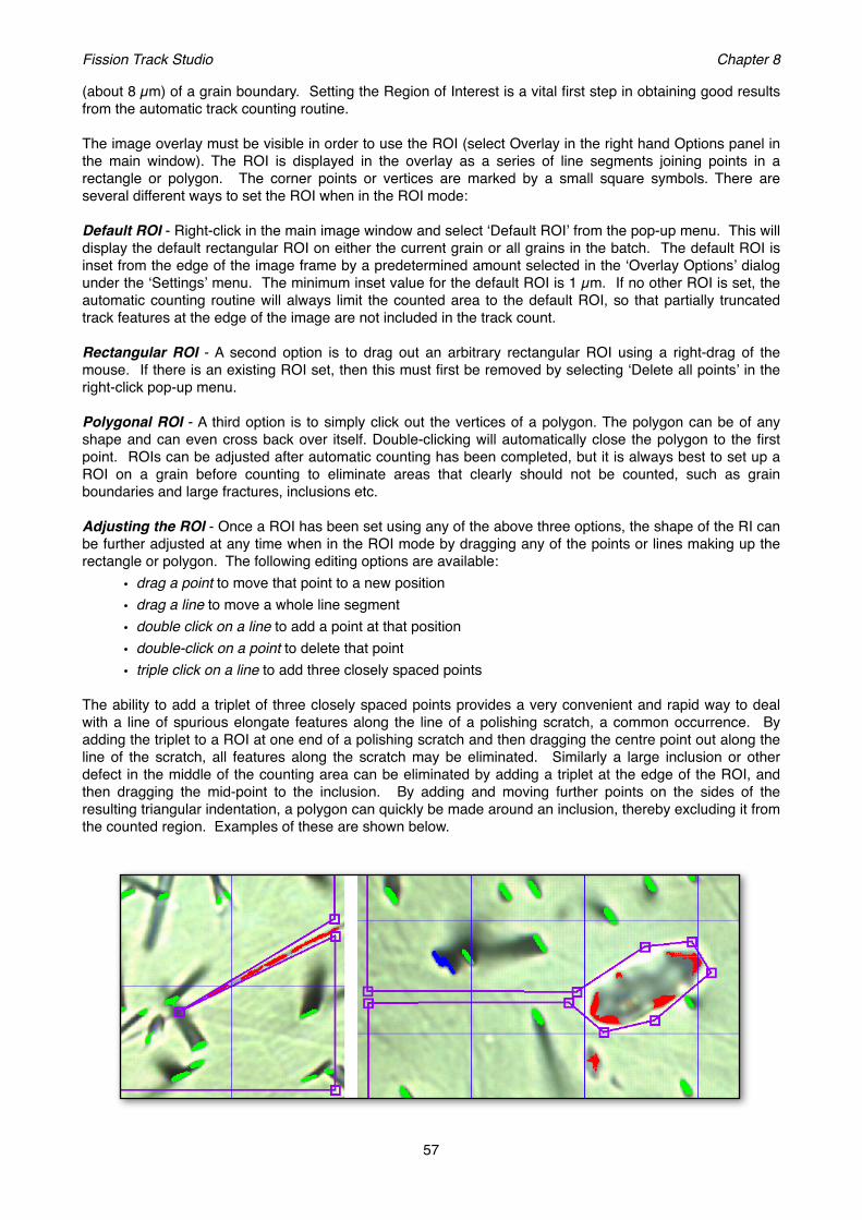
(about 8 µm) of a grain boundary. Setting the Region of Interest is a vital first step in obtaining good results from the automatic track counting routine.

The image overlay must be visible in order to use the ROI (select Overlay in the right hand Options panel in the main window). The ROI is displayed in the overlay as a series of line segments joining points in a rectangle or polygon. The corner points or vertices are marked by a small square symbols. There are several different ways to set the ROI when in the ROI mode:

Default ROI - Right-click in the main image window and select ̒ Default ROIʼ from the pop-up menu. This will display the default rectangular ROI on either the current grain or all grains in the batch. The default ROI is inset from the edge of the image frame by a predetermined amount selected in the ʻOverlay Optionsʼ dialog under the ʻSettingsʼ menu. The minimum inset value for the default ROI is 1 µm. If no other ROI is set, the automatic counting routine will always limit the counted area to the default ROI, so that partially truncated track features at the edge of the image are not included in the track count.

Rectangular ROI - A second option is to drag out an arbitrary rectangular ROI using a right-drag of the mouse. If there is an existing ROI set, then this must first be removed by selecting ʻDelete all pointsʼ in the right-click pop-up menu.

Polygonal ROI - A third option is to simply click out the vertices of a polygon. The polygon can be of any shape and can even cross back over itself. Double-clicking will automatically close the polygon to the first point. ROIs can be adjusted after automatic counting has been completed, but it is always best to set up a ROI on a grain before counting to eliminate areas that clearly should not be counted, such as grain boundaries and large fractures, inclusions etc.

Adjusting the ROI - Once a ROI has been set using any of the above three options, the shape of the RI can be further adjusted at any time when in the ROI mode by dragging any of the points or lines making up the rectangle or polygon. The following editing options are available:

• drag a point to move that point to a new position• drag a line to move a whole line segment• double click on a line to add a point at that position• double-click on a point to delete that point• triple click on a line to add three closely spaced points

The ability to add a triplet of three closely spaced points provides a very convenient and rapid way to deal with a line of spurious elongate features along the line of a polishing scratch, a common occurrence. By adding the triplet to a ROI at one end of a polishing scratch and then dragging the centre point out along the line of the scratch, all features along the scratch may be eliminated. Similarly a large inclusion or other defect in the middle of the counting area can be eliminated by adding a triplet at the edge of the ROI, and then dragging the mid-point to the inclusion. By adding and moving further points on the sides of the resulting triangular indentation, a polygon can quickly be made around an inclusion, thereby excluding it from the counted region. Examples of these are shown below.


57

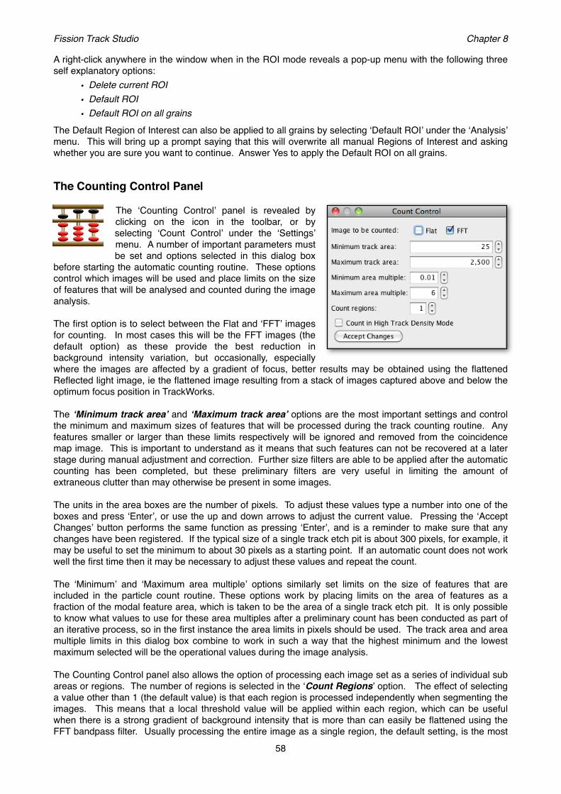
A right-click anywhere in the window when in the ROI mode reveals a pop-up menu with the following three self explanatory options:

• Delete current ROI• Default ROI• Default ROI on all grains

The Default Region of Interest can also be applied to all grains by selecting ̒ Default ROIʼ under the ̒Analysisʼ menu. This will bring up a prompt saying that this will overwrite all manual Regions of Interest and asking whether you are sure you want to continue. Answer Yes to apply the Default ROI on all grains.

The Counting Control Panel

The ʻCounting Controlʼ panel is revealed by clicking on the icon in the toolbar, or by selecting ʻCount Controlʼ under the ʻSettingsʼ menu. A number of important parameters must be set and options selected in this dialog box

before starting the automatic counting routine. These options control which images will be used and place limits on the size of features that will be analysed and counted during the image analysis.

The first option is to select between the Flat and ʻFFTʼ images for counting. In most cases this will be the FFT images (the default option) as these provide the best reduction in background intensity variation, but occasionally, especially where the images are affected by a gradient of focus, better results may be obtained using the flattened Reflected light image, ie the flattened image resulting from a stack of images captured above and below the optimum focus position in TrackWorks.

The ʻMinimum track areaʼ and ʻMaximum track areaʼ options are the most important settings and control the minimum and maximum sizes of features that will be processed during the track counting routine. Any features smaller or larger than these limits respectively will be ignored and removed from the coincidence map image. This is important to understand as it means that such features can not be recovered at a later stage during manual adjustment and correction. Further size filters are able to be applied after the automatic counting has been completed, but these preliminary filters are very useful in limiting the amount of extraneous clutter than may otherwise be present in some images.

The units in the area boxes are the number of pixels. To adjust these values type a number into one of the boxes and press ʻEnterʼ, or use the up and down arrows to adjust the current value. Pressing the ʻAccept Changesʼ button performs the same function as pressing ʻEnterʼ, and is a reminder to make sure that any changes have been registered. If the typical size of a single track etch pit is about 300 pixels, for example, it may be useful to set the minimum to about 30 pixels as a starting point. If an automatic count does not work well the first time then it may be necessary to adjust these values and repeat the count.

The ʻMinimumʼ and ʻMaximum area multipleʼ options similarly set limits on the size of features that are included in the particle count routine. These options work by placing limits on the area of features as a fraction of the modal feature area, which is taken to be the area of a single track etch pit. It is only possible to know what values to use for these area multiples after a preliminary count has been conducted as part of an iterative process, so in the first instance the area limits in pixels should be used. The track area and area multiple limits in this dialog box combine to work in such a way that the highest minimum and the lowest maximum selected will be the operational values during the image analysis.

The Counting Control panel also allows the option of processing each image set as a series of individual sub areas or regions. The number of regions is selected in the ʻCount Regionsʼ option. The effect of selecting a value other than 1 (the default value) is that each region is processed independently when segmenting the images. This means that a local threshold value will be applied within each region, which can be useful when there is a strong gradient of background intensity that is more than can easily be flattened using the FFT bandpass filter. Usually processing the entire image as a single region, the default setting, is the most


58

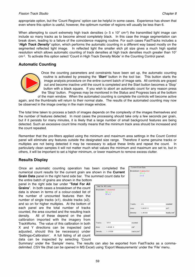
appropriate option, but the ʻCount Regionsʼ option can be helpful in some cases. Experience has shown that even where this option is useful, however, the optimum number of regions will usually be less than 6.

When attempting to count extremely high track densities (> 5 x 107 cm-2) the transmitted light image can include so many tracks as to become almost completely black. In this case the image segmentation can break down, leading to a failure of the coincidence mapping routine. For such cases FastTracks includes a ʻHigh Track Densityʼ option, which performs the automatic counting in a different way based mostly on the segmented reflected light image. In reflected light the smaller etch pit size gives a much high spatial resolution which allows automatic counting of track densities at high track densities much greater than 107 cm-2. To activate this option select ʻCount in High Track Density Modeʼ in the Counting Control panel.

Automatic Counting

Once the counting parameters and constraints have been set up, the automatic counting routine is activated by pressing the ʻStartʼ button in the tool bar. This button starts the image analysis procedure on the entire current batch of image sets. All controls are grayed out and become inactive until the count is completed and the Start button becomes a ʻStopʼ button with a black square. If you wish to abort an automatic count for any reason press

the ʻStopʼ button. Progress may be monitored in the Status and Progress bars at the bottom of the main window. When the automated counting is complete the controls will become active

again, and the thumbnails will return to their normal state. The results of the automated counting may now be observed in the image overlay in the main image window.

The total time taken to process a batch of images depends on the complexity of the images themselves and the number of features detected. In most cases the processing should take only a few seconds per grain, but if it persists for many minutes, it is likely that a large number of small background features are being detected. Such an excessive count time mostly means that the minimum track area should be increased and the count repeated.

Remember that the pre-filters applied using the minimum and maximum area settings in the Count Control panel will eliminate any features outside the designated size range. Therefore if some genuine tracks or multiples are not being detected it may be necessary to adjust these limits and repeat the count. In particularly clean samples it will not matter much what values the minimum and maximum are set to, but in others, it will be important to set a higher minimum, or lower maximum to remove excess clutter. #

Results Display

Once an automatic counting operation has been completed the numerical count results for the current grain are shown in the Current Grain Data panel in the right hand side bar. The summed count data for the entire batch of grains are shown in the bottom panel in the right side bar under “Total For All Grains”. In both cases a breakdown of the count data is shown in terms of a colour-coded list of the number of uncounted features then the number of single tracks (x1), double tracks (x2), and so on for higher multiples. At the bottom of each panel are the total number of tracks counted, the area counted and the resulting track density. All of these depend on the pixel calibration imported with the imagery from TrackWorks. The value of this calibration in both X and Y directions can be inspected (and adjusted, should this be necessary) under ʻSettings>Calibrationʼ. A full listing of all count data can be inspected by selecting ʻCount Summaryʼ under the ʻSampleʼ menu. The results can also be exported from FastTracks as a comma-delimited .CSV file (that can be opened in MS Excel) using ʻExport Measurementsʼ under the ʻFileʼ menu.


59

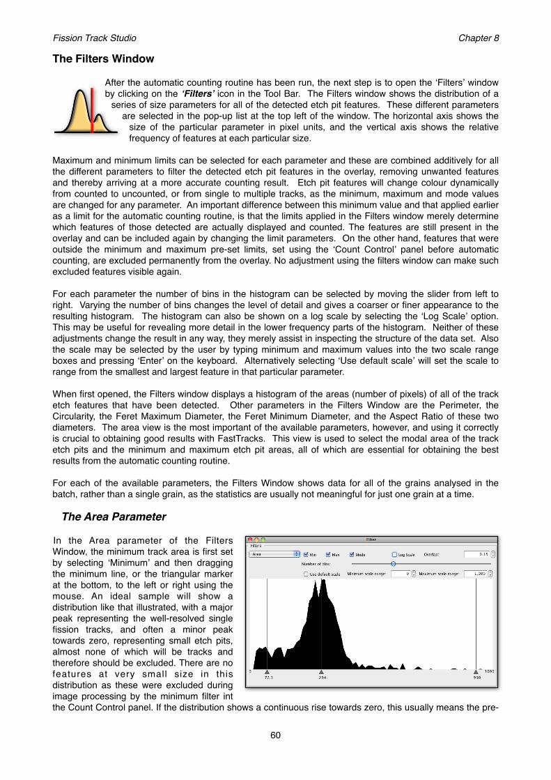
The Filters Window

After the automatic counting routine has been run, the next step is to open the ʻFiltersʼ window by clicking on the ʻFiltersʼ icon in the Tool Bar. The Filters window shows the distribution of a

series of size parameters for all of the detected etch pit features. These different parameters are selected in the pop-up list at the top left of the window. The horizontal axis shows the

size of the particular parameter in pixel units, and the vertical axis shows the relative frequency of features at each particular size.

Maximum and minimum limits can be selected for each parameter and these are combined additively for all the different parameters to filter the detected etch pit features in the overlay, removing unwanted features and thereby arriving at a more accurate counting result. Etch pit features will change colour dynamically from counted to uncounted, or from single to multiple tracks, as the minimum, maximum and mode values are changed for any parameter. An important difference between this minimum value and that applied earlier as a limit for the automatic counting routine, is that the limits applied in the Filters window merely determine which features of those detected are actually displayed and counted. The features are still present in the overlay and can be included again by changing the limit parameters. On the other hand, features that were outside the minimum and maximum pre-set limits, set using the ʻCount Controlʼ panel before automatic counting, are excluded permanently from the overlay. No adjustment using the filters window can make such excluded features visible again.

For each parameter the number of bins in the histogram can be selected by moving the slider from left to right. Varying the number of bins changes the level of detail and gives a coarser or finer appearance to the resulting histogram. The histogram can also be shown on a log scale by selecting the ʻLog Scaleʼ option. This may be useful for revealing more detail in the lower frequency parts of the histogram. Neither of these adjustments change the result in any way, they merely assist in inspecting the structure of the data set. Also the scale may be selected by the user by typing minimum and maximum values into the two scale range boxes and pressing ʻEnterʼ on the keyboard. Alternatively selecting ʻUse default scaleʼ will set the scale to range from the smallest and largest feature in that particular parameter.

When first opened, the Filters window displays a histogram of the areas (number of pixels) of all of the track etch features that have been detected. Other parameters in the Filters Window are the Perimeter, the Circularity, the Feret Maximum Diameter, the Feret Minimum Diameter, and the Aspect Ratio of these two diameters. The area view is the most important of the available parameters, however, and using it correctly is crucial to obtaining good results with FastTracks. This view is used to select the modal area of the track etch pits and the minimum and maximum etch pit areas, all of which are essential for obtaining the best results from the automatic counting routine.

For each of the available parameters, the Filters Window shows data for all of the grains analysed in the batch, rather than a single grain, as the statistics are usually not meaningful for just one grain at a time.

The Area Parameter

In the Area parameter of the Filters Window, the minimum track area is first set by selecting ʻMinimumʼ and then dragging the minimum line, or the triangular marker at the bottom, to the left or right using the mouse. An ideal sample will show a distribution like that illustrated, with a major peak representing the well-resolved single fission tracks, and often a minor peak towards zero, representing small etch pits, almost none of which will be tracks and therefore should be excluded. There are no features at very small size in this distribution as these were excluded during image processing by the minimum filter int the Count Control panel. If the distribution shows a continuous rise towards zero, this usually means the pre-


60

filter minimum should be set to a higher value and the automatic count run again see above under Counting Control Panel).

While looking at the track image and overlay in the main window, slide the minimum value to eliminate the smallest features in the overlay image that are clearly not fission tracks. These should turn red (the default colour for uncounted features) as the minimum value exceeds their actual areas. If the overlay visibility for ʻUncounted tracksʼ is not selected in ʻSettings >Overlay Optionsʼ, these tracks will disappear when they are less than the minimum area, rather than turning red.

Once the minimum track area has been set, the next step is to click on the Mode option to show a default estimate of the modal track pit area. This estimated mode is determined as the mid point of the main peak at half its height. Obviously this default mode estimate only works where there is a well-defined peak as illustrated. In some samples having a lot a small features, or perhaps a low track density, the mode may appear close to zero, in which case it will be important to set the minimum value first, and then adjust the mode manually by dragging the mode line or the small triangular handle at the bottom. The modal area value is a key parameter in determining which features are track multiples in the overlay. The mode should therefore be adjusted manually while looking at the track and overlay images in the main window so that clearly single tracks are represented that way, and double, or higher, multiples are also correctly identified. This method of discriminating multiples is very effective but does not work perfectly in every case, so there will always be some degree of mis-identification. A judgement is therefore needed as to which will be the optimum value for the mode for each sample so as to minimize any errors.

The area based multiple-discrimination works well because over the greater part of the range of countable track densities, the overlap of individual etch pits in the Coincidence map is actually quite small, although in most cases not zero. An average degree of track overlap may also be set in the Filters window the box in the top right of the panel, and the default value of 0.15 (15%) works well in most cases. For higher track densities a higher degree of average overlap may be appropriate. The image analysis assumes that double track etch pits will on average have an area twice the modal value for single tracks, less the overlap proportion. This simple technique, although effective, is not perfect and some manual adjustment of the results may be necessary at the final review and editing stage. It does not work at all well if grains have been selected that do not have their surfaces close to parallel to the c-axis. In such grains tracks lying in different orientations have very different etch pit areas, and this method of estimating multiples breaks down.

In the same way, a maximum value can be set for the etch pit area. This is useful to eliminate unwanted clutter from large defects in the grain images, such as fractures, inclusions and the like. In most samples, higher-order multiples will be rare, so it is possible to reduce the maxim limit to perhaps three or four times the modal value. For higher track densities with more higher-order multiples, a greater maximum limit will need to be used. For all of these parameters, it is good to check the result on several different grains to check that the parameters have been set in a way that correctly discriminates between tracks and non-track features and between single and multiple tracks. In a very diverse set of grains, the settings will necessarily be something of a compromise between the best settings for individual grains.

Using the Area Filter


61

Min Max

An example may help to illustrate the the importance and effectiveness of applying the Area Filters. The image on the left above shows a coincidence map resulting from a very noisy fission track image, including an unusually large number of polishing scratch features, a large inclusion (roughly hexagonal in outline at top centre), as well as several large fractures. On the right is the resulting Area filter histogram showing the size distribution of all the features in this image. Inspecting the histogram shows that three distinct components can be identified, with the large peak on the left hand side representing a numerous small features that have been detected, mostly relating to the polishing scratches. The much lower peak in the centre represents the fission tracks, and the third peak, on the far right shows several large defects made up of the fractures and features related to the inclusion. Setting the minimum filter as indicated in the histogram above deletes all of the smaller features resulting in the following image on the left below, and applying the maximum filter similarly eliminates all of the large features leaving the image on the right below. This final image consist mostly of fission tracks with a few remaining defects that can be removed by using the Region of Interest tool, by manual editing, or by using one of the other filter parameters as described below.

Feret Maximum, Feret Minimum

Selecting the Feret Maximum parameter in the Filters Window pop-up shows a different histogram summarizing the maximum diameters of all of the detected etch pits. The Feret diameters are defined as the distance between two parallel tangents to the perimeter of a particle, that are respectively the maximum and minimum possible. In a well selected apatite grain, with the surface cut closely parallel to c, the Feret Maximum diameters for the single track etch pits will all define a similar direction, representing azimuth direction of the c-axis in the section plane.

An important use for use for the Feret Maximum Filter is to select well-resolved, single track etch pits that are most useful for determining the kinetic parameter Dpar (etch pit diameter perpendicular to the c-axis). Dpar can be estimated automatically using this Filter window, or manually using the measurement tools described in Chapter 6. To make an automatic measurement the first step is to select and adjust the Mode in the Feret Maximum filter. Once the Mode is set, the value of Dpar is displayed in the window in microns, and will also appear in the data export file. A typical example is shown in which there is a well defined modal peak representing the most common Feret Maximum value. This value, 32.4 pixels in the example shown, multiplied by the pixel calibration, provides an estimate of Dpar, 1.79 microns in this particular case. In most cases this estimate will be based on a substantial number of individual tracks and is likely to be more precise than a manual measurement based on just a few etch pits.

If a manual Dpar measurement is to be made, the minimum and maximum values can be used to better define the lower and upper bounds of this peak and thereby to highlight the single track etch pits in the


62

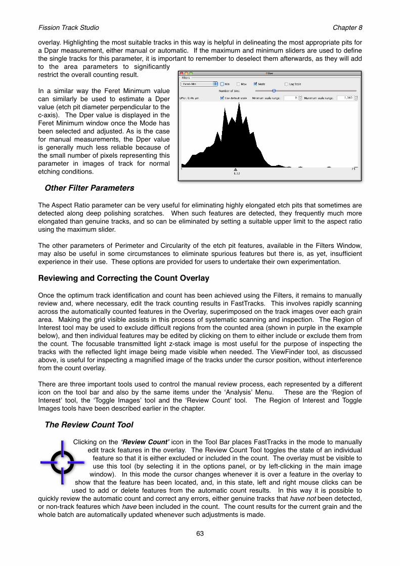
overlay. Highlighting the most suitable tracks in this way is helpful in delineating the most appropriate pits for a Dpar measurement, either manual or automatic. If the maximum and minimum sliders are used to define the single tracks for this parameter, it is important to remember to deselect them afterwards, as they will add to the area parameters to significantly restrict the overall counting result.

In a similar way the Feret Minimum value can similarly be used to estimate a Dper value (etch pit diameter perpendicular to the c-axis). The Dper value is displayed in the Feret Minimum window once the Mode has been selected and adjusted. As is the case for manual measurements, the Dper value is generally much less reliable because of the small number of pixels representing this parameter in images of track for normal etching conditions.

Other Filter Parameters

The Aspect Ratio parameter can be very useful for eliminating highly elongated etch pits that sometimes are detected along deep polishing scratches. When such features are detected, they frequently much more elongated than genuine tracks, and so can be eliminated by setting a suitable upper limit to the aspect ratio using the maximum slider.

The other parameters of Perimeter and Circularity of the etch pit features, available in the Filters Window, may also be useful in some circumstances to eliminate spurious features but there is, as yet, insufficient experience in their use. These options are provided for users to undertake their own experimentation.

Reviewing and Correcting the Count Overlay

Once the optimum track identification and count has been achieved using the Filters, it remains to manually review and, where necessary, edit the track counting results in FastTracks. This involves rapidly scanning across the automatically counted features in the Overlay, superimposed on the track images over each grain area. Making the grid visible assists in this process of systematic scanning and inspection. The Region of Interest tool may be used to exclude difficult regions from the counted area (shown in purple in the example below), and then individual features may be edited by clicking on them to either include or exclude them from the count. The focusable transmitted light z-stack image is most useful for the purpose of inspecting the tracks with the reflected light image being made visible when needed. The ViewFinder tool, as discussed above, is useful for inspecting a magnified image of the tracks under the cursor position, without interference from the count overlay.

There are three important tools used to control the manual review process, each represented by a different icon on the tool bar and also by the same items under the ʻAnalysisʼ Menu. These are the ʻRegion of Interestʼ tool, the ʻToggle Imagesʼ tool and the ʻReview Countʼ tool. The Region of Interest and Toggle Images tools have been described earlier in the chapter.

The Review Count Tool

Clicking on the ʻReview Countʼ icon in the Tool Bar places FastTracks in the mode to manually edit track features in the overlay. The Review Count Tool toggles the state of an individual

feature so that it is either excluded or included in the count. The overlay must be visible to use this tool (by selecting it in the options panel, or by left-clicking in the main image

window). In this mode the cursor changes whenever it is over a feature in the overlay to show that the feature has been located, and, in this state, left and right mouse clicks can be

used to add or delete features from the automatic count results. In this way it is possible to quickly review the automatic count and correct any errors, either genuine tracks that have not been detected, or non-track features which have been included in the count. The count results for the current grain and the whole batch are automatically updated whenever such adjustments is made.


63

When in the Count Tracks mode, the various editing options are as follows:• a left-click on an existing feature toggles it between the counted and uncounted states. This is most

commonly used to delete a spurious feature that has been included in the automatic count. Clicking again will restore that feature to the count.

• a left-click outside an existing feature will add a small cross in the overlay at that point and increase the count by one. Clicking on this cross again will delete the cross and reduce the count accordingly.

• a right-click on an existing feature displays a pop-up menu (illustrated below) enabling the multiple status of that feature to be seen, and another value chosen. Select 2 for a double track, 3 for a triple, etc. The status of a multiple track can be returned to a single by right-clicking on it and reducing its multiple status to 1.

• a right-click away from an existing feature will add a small cross at that point and display a pop-up menu allowing the multiple status to be selected.

During manual editing it is frequently useful to focus the z-stack image using the mouse scroll wheel and to switch the reflected light layer on and off, which is normally achieved with a right-click in the Toggle Images Mode. Because the Toggle Images and Count Tracks modes cannot be operated simultaneously, FastTracks has a series of keystroke commands that temporarily switch between these modes. This can be done by leaving FastTracks in the Toggle Images mode (by clicking the ʻToggle Imagesʼ icon in the Tool Bar) and pressing the Control key, to edit tracks. This will switch to the Count Tracks mode for as long as the Control key is depressed. Scanning can then be done in the Toggle Images mode, using left and right-clicks to switch the overlay and reflected light layers on and off, and then using the Control key to activate the Count Tracks mode when needed. WIth practice, this use of the Control key makes for the fastest means for quickly switching images views and manually editing track features.

Hot Keys

A number of other keystroke options are also available to quickly switch between the various viewing and measurement modes. These ʻHot Keysʼ and their resulting actions are listed in the following table.

Hot Key Action

Ctrl + Space Toggle overlay visibility on and off

Shift + Space Toggle reflected light image visibility on and off

Ctrl + Left-Click Toggle individual track or count new track

Ctrl + Right-Click Set multiple track count

Shift + Left-Click Measure length manually

Shift + Right-Click Delete a manual length

Ctrl + Shift + Left-Click Measure C-Axis manually

Ctrl + h Show/hide uncounted features

Ctrl + g Show/hide grid


64

Overlay Options

A number of different features and measurements may be shown in the Overlay layer and the set of features visible at any time may be controlled using the Overlay Options dialog box. This panel may be selected using the ʻSettings>Overlay Optionsʼ menu item. Mostly these options operate the same way in FastTracks as they do in TrackWorks, as described in Chapter 6. Using the overlay options it is possible to show or hide various features in the overlay and to set some overlay properties.

These options include:• ʻTracksʼ can be used to show/hide all track features in the overlay. Hiding the tracks may be useful

when making measurements of track lengths etc using the measurement tools.• ʻFill Track Overlayʼ - displays features as solid colour,

rather than outlines. This is the default setting and usually the most useful as it maximizes the visibility of the identified features.

• ʻUncounted tracksʻ - makes features that have been excluded using the filters or manual editing visible or invisible. If selected, uncounted features are visible (in the ʻuncountedʼ colour). This has no effect on the counting result, merely on the visibility.

• ʻRegion of Interest, CAxis, Lengths, and Dpars/Dpersʼ make these different content layers visible when selected.

• Display scale barʼ shows the scale bar.• ʻOverlay Line Width ̓ - adjusts the thickness of

different lines in the overlay, including the ROI, c-axis track lengths and Dpar measurements. This can aid visibility.

• ʻDefault ROI Insetʼ - changes the value in microns by which the default Region of Interest is set in from the edge of the image field. This value must be 1 or more.

Other tabs in the Overlay Options window allow the colours used for various different image features to be set and the cursor type to be selected, as described in detail in Chapter 6.

Problem tracks

While FastTracks does an excellent job of identifying and counting most fission tracks in typical apatite samples, there is a class of shallow-dipping tracks which it has trouble identifying accurately. These shallow-dipping tracks usually make up only a very small proportion of the total tracks present (~2.5%), but they are either missed by the automatic counting routine altogether in the most extreme cases, or are revealed as two separate etch pit features. The resulting counting errors from these ʻproblemʼ tracks are even less as the missed tracks partially compensate for the double features, giving an apparent error rate of only about 1.5% from these features if no correction were made. The characteristics of these shallow dipping tracks are illustrated below.

The upper row shows a idealized view of the tracks themselves at various angles from near vertical on the left to very shallow dipping on the right. The bottom row shows the features that result in the overlay from coincidence mapping during the automatic counting routine. In the case of the shallowest dipping tracks at the right, bright reflections are seen from the facets of the track edges in the wide mouth of the track opening. These sometimes result in such features not being

detected by the coincidence mapping routine, as highlighted on the right. For less shallow-dipping tracks two features will often be seen in the processed overlay as highlighted second from right. Two examples of


65

these double etch pit features are shown in the image overlay on the right, and several more may be seen in the main window illustrated above under ʻReview Count Toolʼ. Although the errors from miscounting such features are small and partly self-compensating, they are common enough, and distinctive enough, that it is quite simple to look out for them and to manually correct the errors that result, either by deleting one of the twin etch features or adding a count for those tracks that are missed entirely. Future developments will seek to find an automated solution to identifying this class of problematic track etch features.

View and Export Results

Once the observer is satisfied with the counting results they can be inspected in tabulated form using the ʻCount Summaryʼ command under the ʻSampleʼ menu. The counting results can then be exported using the ʻExportʼ command under the ʻFileʼ menu. This exports a comma-delimited .CSV file that can be opened in MS Excel for further processing and analysis. If other measurements have been made using the c-axis, track length and Dpar tools,then the entire data set may be exported in tabulated form as a .CSV file using the ʻExport Measurementsʼ command under the ʻFileʼ menu. These measurement tools operate exactly the same way as they do in TrackWorks as described in Chapter 6.


66

The software now comes with support for piercing proxies. If you cannot download the latest version of the software, it is likely that you are behind a proxy. To get around the proxy, you must first check the “Use proxy settings” box, and then fill the proxy address and proxy port fields. If you do not know the proxy address or port, request the assistance of the IT staff, who should be able to assist you. Once you have filled the “Proxy address” and “Proxy port” textbox, you can either restart the software, provided that “Check for updates on startup” is enabled, or click on the “Check for Updates” button if working in FastTracks.

In the “Enter authentication details” dialog box, you must enter your default username and password. This will be the same as the username and password you need to use the internet browser. Once this is completed, the updater should work correctly. If an error similar to “HTTP error: 407” displays, it is likely that the authentication details were inputted incorrectly.

Fission Track Studio - Trinity College, Dublin Track... · Both programs contain a common set of...

Documents

Transcript of Fission Track Studio - Trinity College, Dublin Track... · Both programs contain a common set of...