DP/90/2013

Fiscal Policy and EconomicGrowth in Bulgaria

Kristina Karagyozova-MarkovaGeorgi Deyanov

Viktor Iliev

DISCUSSION PAPERSDP/90/2013

December 2013

DISCUSSION PAPERS

Fiscal Policy and Economic Growth in Bulgaria

Kristina Karagyozova-Markova, Georgi Deyanov, Viktor Iliev

BULGARIANNATIONAL

BANK

2

DP

/90/

2013

DISCUSSION PAPERSEditorial Board:Chairman: Ass. Prof. Statty Stattev, Ph. D.Members: Kalin Hristov Tsvetan Manchev, Ph. D. Ass. Prof. Mariella Nenova, Ph. D. Ass. Prof. Pavlina Anachkova, Ph. D. Andrey Vassilev, Ph. D. Daniela Minkova, Ph. D.Secretary: Lyudmila Dimova

© Kristina Karagyozova-Markova, Georgi Deyanov, Viktor Iliev, 2013© Bulgarian National Bank, series, 2013

ISBN 978–954–8579–50–6

Printed in the BNB Printing Centre.

Elements of the 1999 banknote with a nominal value of 50 levs are used in cover design.

Send your comments and opinions to:Publications DivisionBulgarian National Bank1, Knyaz Alexander I Square1000 Sofia, BulgariaTel.: (+359 2) 9145 1351, 9145 1978Fax: (+359 2) 980 2425e–mail: Dimova.L@bnbank.orgWebsite: www.bnb.bg

3

DIS

CU

SS

ION

PA

PE

RS

Contents

Introduction ................................................................................... 5Overview of related literature ................................................. 6Definition of fiscal multipliers .................................................. 6Determinants of fiscal multipliers ........................................... 7Time-variation in fiscal multipliers .......................................... 8The size of fiscal multipliers ..................................................... 9

Overview of the estimation techniques ................................10Linear VAR Models ..................................................................11Non-linear VAR Models ..........................................................13

Data Description ........................................................................14

Models Description ...................................................................15The recursive approach ..........................................................15The approach of Blanchard and Perotti ..............................16Time-varying parameter VAR model ....................................18

Results ...........................................................................................19Time-invariant fiscal multipliers .............................................19Time-varying fiscal multipliers ...............................................21Conclusions, policy implications and further work ..........30

References ...................................................................................33

Appendix A. Details on data ....................................................37

Appendix B. Details on the econometric methodology ....39

Appendix C. Details on the derivation of tax revenue elasticity ........................................................................................44

Appendix D. Impulse responses from the baseline VAR models .................................................................................47

Appendix E. Robustness check ................................................51

Appendix F. Supplementary figures and tables....................57

4

DP

/90/

2013

SUMMARY: This paper analyses the impact of fiscal policy on economic activity in Bulgaria and provides a range of estimates for the tax and spend-ing multipliers. We compare the results of linear VAR models with the output from time-varying parameters Bayesian VAR with stochastic volatility. In all model specifications, first-year spending multipliers do not exceed 0.4, imply-ing that there is not much to gain in terms of economic output from demand stimulating fiscal policy in Bulgaria. There is a lot of uncertainty in regards to the size of the tax multipliers, given contrasting results from VARs with different identification techniques, but the overall output effect of tax meas-ures appears to be small and short-lived. The results from the linear models are largely consistent with the output from the time-varying parameters VAR model, which indicates that the size of first-year spending multiplier has dou-bled during the recent global crisis, but remains no larger than 0.3. These findings support the general view in the literature that fiscal multipliers are higher during periods of economic recession, but they are typically small in small open economies.

Keywords: Fiscal policy, Structural VAR models, Fiscal multipliers, Govern-ment spending, Bayesian estimation, Time-varying parameters

JEL Codes: C11, C32, E62

The authors would like to thank Mariella Nenova, Andrey Vassilev, Tsvetan Man-chev and the members of the editorial board of the Bulgarian National Bank Discus-sion Papers for their helpful comments and suggestions. They are especially indebted to Dr. Haroon Mumtaz for providing valuable technical guidance. Comments and feedback received at different stages from all colleagues at the Economic Research and Forecasting Department of the Bulgarian National Bank are also greatly acknowl-edged. Corresponding author e-mail: Kristina Karagyozova, Karagyozova.K@bnbank.org. The views expressed herein are those of the authors and do not necessarily rep-resent the views of the Bulgarian National Bank. All remaining errors in the paper are solely the responsibility of the authors.

5

DIS

CU

SS

ION

PA

PE

RS

IntroductionThe strand of literature researching the effect of fiscal policy on the

economy has gained momentum after the 2007/2008 global financial tur-moil. While initially the main question for the policy makers was about the size and appropriate mix of fiscal stimuli to counteract the severe economic downturn, sovereign debt sustainability issues soon moved the focus of the discussion on fiscal consolidation strategies and the quantification of the ex-pected negative effects on output. In both cases, however, the output ef-fects of fiscal policy, as measured by the fiscal multiplier, are in the center of the discussion. Broadly speaking, the fiscal multiplier is used to measure the overall effect of discretionary fiscal policy on economic output. In 2012 the debate on the size of the fiscal multipliers has become even more rele-vant, as the economic recovery was weaker than expected in most European countries and the euro area fell into recession for a second time.

Despite its high importance and the large number of research papers published in recent years, the discussion regarding the macroeconomic ef-fects of fiscal policy remains a highly controversial one. In fact, there is no theoretical consensus on the size and even the sign of the fiscal multipliers, with neoclassical and new Keynesian macroeconomic models predicting dif-ferent responses of private consumption, employment and real wages, fol-lowing a fiscal shock. The numerous studies published since the onset of the global crisis did not manage to provide firm support for either of the theoreti-cal models. On the contrary, the estimates of the size of the fiscal multipliers are now dispersed over an even broader range, which is largely due to the lack of consensus on the most appropriate way of their assessment.

The aim of this paper is to contribute to the analysis and the debate on the macroeconomic effects of fiscal policy by providing a range of estimates for the fiscal multipliers in Bulgaria. For the purpose, we estimate several linear and time-varying parameter vector autoregressive models. Our con-tribution to the existing body of literature is twofold. First, the paper adds to a small but growing literature on the effects of fiscal policy in Central and Eastern Europe and Bulgaria in particular, by applying methodologies that have been found useful in assessing fiscal multipliers in the more advanced European economies. Second, we contribute to the relatively new and so far limited research effort of employing time-varying parameter VAR models to study the output effects of fiscal policy over time. We consider the ap-plication of this methodology to be especially relevant for analyzing fiscal policy in Eastern European economies, where many factors for non-linearity and time-dependent effects of fiscal stimuli have been present in the last 15 years.

6

DP

/90/

2013

The rest of the paper is structured as follows: the next section provides a brief overview of the related literature, including useful definitions and list of the main factors that affect the multipliers’ size and their variation over time; Section 3 briefly presents the mostly widely used evaluation method-ologies for measuring fiscal multipliers and reviews the different techniques for identification of fiscal policy shocks; Section 4 and Section 5 describe the data and the models that we use in the empirical study; Section 6 presents the results, while Section 7 is dedicated to the concluding remarks and the policy implications of the results.

Overview of related literature

Definition of fiscal multipliers

A brief overview of the related publications points to the conclusion that the fiscal multipliers are found in many different forms in the academic lit-erature and their size varies considerably even if the analyses are focused on a specific economy, region and time span. In this study, along with the common practice, the fiscal multiplier is measured by the ratio of the change in GDP, or other measure of output, to the exogenous change in a fiscal variable that has caused the effect on output. For example, the spending multiplier represents the change of GDP due to a discretionary increase of government spending (fiscal shock). Thus, if the fiscal multiplier is higher or smaller than unity, fiscal expansion would respectively crowd-in or crowd-out some component of aggregate demand and consequently output. Depend-ing on the fiscal variable that is chosen for the assessment, the multiplier could be defined as government consumption multiplier, government invest-ment multiplier, tax multiplier (which can be further broken down to direct or indirect tax multiplier, net tax multiplier etc.), lump-sum transfers multiplier, etc. Also, the definition of the fiscal multipliers may differ according to the period of time considered in the assessment. For instance, the impact multi-plier refers to the estimated ratio in the first period (e.g. first quarter) follow-ing the fiscal shock, while the cumulative multiplier refers to the ratio of the cumulative changes in the output and the fiscal variable over a specified time horizon (Spilimbergo et al., 2009). Short-, medium- and long-term multipliers are also frequently used notions in the literature. Short-term multipliers usu-ally provide a measure of the output effects up to one year after the fiscal shock has taken place, while the medium-term multipliers are typically calcu-lated for a period between 1 and 3 years.

7

DIS

CU

SS

ION

PA

PE

RS

Determinants of fiscal multipliers

Overall, there is a broad consensus in the academic literature about the main factors that affect the size of the fiscal multipliers. Spilimbergo et al. (2009) have grouped the most relevant of them.

First, fiscal multipliers are considered to be larger when only a small part of the additional income generated by the fiscal stimulus is saved by the private sector or used for imported goods and services (thus limiting the negative effect on output resulting from lower consumption or higher im-ports). These conditions are particularly valid when: the economy is large or relatively closed (i.e. the marginal propensity to import is relatively small); the structure of the stimulus is such that it does not affect imports and it is mostly based on an increase in government expenditure, rather than a decrease in taxes;1 the marginal propensity to consume is high and the stimulus is tar-geted towards credit or liquidity constrained consumers (i.e. hand-to-mouth consumers); following fiscal stimulus the economic agents do not expect fu-ture offsetting measures due to short planning horizon or poorly formulated expectations for the future (i.e. non-Ricardian households);2 the automatic stabilizers are small3 and the efficiency of public spending is high.

Second, the size of the fiscal multiplier, at least theoretically, depends on the monetary policy response to the fiscal shock (expansion). The traditional argument in the literature follows the Mundell-Fleming proposition, which implies that fiscal multipliers are lower in economies with floating exchange rates regimes. Born et al. (2012) discuss the relevance of the Mundell-Flem-ing proposition in explaining the size of fiscal multipliers and its empirical validity. The authors conclude that the difference between the size of the spending multipliers in economies under fixed and floating exchange rate are smaller than what the traditional Mundell-Fleming analysis would suggest.

The sustainability of the fiscal stance after the stimulus is another impor-tant determinant of the multiplier’s size. Excessively high or rapidly rising gov-

1 The increase in government expenditure usually has a more direct effect on aggregate demand (increase in social transfers in kind, government purchases of goods and services etc.), while the additional income from a tax decrease might be saved by the consumers, thus limiting the second round effects on aggregate demand.

2 I.e., the economic agents do not expect an increase in taxes in the future as a result of fiscal stimulus today. Therefore, the agents would rather spend the additional income, resulting from the stimulus, rather than increase precautionary savings in anticipation of higher taxation in the future. In the case when the Ricardian equivalence is valid, private saving would offset the effects from the expansionary fiscal policy, especially if the fiscal shock is permanent.

3 Smaller automatic stabilizers are associated with relatively smaller output elasticity of govern-ment revenue and spending. Therefore, the automatic offset effect, resulting from the fiscal stimulus, would be more limited.

8

DP

/90/

2013

ernment debt levels might negatively affect the effectiveness of fiscal policy in stimulating economic output, as demonstrated by Kirchner et al. (2010) and Nickel and Tudyka (2013). Considering the increasing or already high level of public indebtedness, private agents would perceive the present fiscal situation as unsustainable. Therefore, the fiscal stimulus would lead to lower private consumption and higher precautionary savings, as agents expect higher taxes or lower government consumption in the future, as a result of the higher deficit today. Such argument is strongly supported in the literature on expansionary fiscal contractions (Giavazzi and Pagano, 1990)4 and it is to a large extent supported by the latest developments in the EU.

More recent studies have found that the degree of financial market de-velopment of the country could also affect the size of the fiscal multipliers. Limited credit availability would result in higher share of liquidity-constrained households and companies, which would spend the additional income, as-sociated with the fiscal stimulus, in order to smooth their consumption or investment needs.

Time-variation in fiscal multipliers

The assessment of the fiscal multipliers becomes even more complicated, especially in the current economic environment, by the fact that their size (and possibly the sign) varies over time. Indeed, subsample instability has often been observed in the recent empirical studies (e.g. Pereira and Lopes, 2010). Specifically, the size of the fiscal multipliers is found to be depend-ent on the underlying state of the economy, as argued by Spilimbergo et al (2009), Baum and Koester (2011, 2012) and Auerbach and Gorodnichenko (2010, 2011). In most cases, fiscal multipliers tend to be larger in downturns than in expansions. This asymmetry has important fiscal policy implications, especially regarding the choice between frontloading and back-loading the required fiscal consolidation effort. Nevertheless, there are several sources of the economic-state dependent character of the multipliers that should be considered when choosing the appropriate adjustment strategy.

On the one hand, fiscal multipliers might be larger in periods of econom-ic recessions since the negative output gap allows the monetary authority to accommodate the increase in demand (as a result of expansionary fiscal measures) without having to increase interest rates, which would otherwise

4 Giavazzi and Pagano (1990) find empirical relevance for expansionary effects of fiscal contrac-tion for the case of Denmark in the 80’s where cuts in government spending were associated with an increase in consumption even after controlling for wealth and income, and even in the presence of a substantial increase in current taxes.

9

DIS

CU

SS

ION

PA

PE

RS

offset part of the fiscal stimuli effects. In the opposite case, the monetary au-thority would not increase the money supply as a response to the increase in output due to the associated inflationary pressure. This, in turn would appre-ciate the local currency (due to increase in interest rates and capital inflows) and reduce net exports, hence, offsetting the initial fiscal expansion effect on output. Under a fixed exchange rate, however, the fiscal expansion would im-ply increase in money demand and a corresponding increase in money sup-ply, with no offsetting effect through a decrease in net exports. Moreover, the share of liquidity and/or credit constrained households and companies usually increases in downturns and allows for a much stronger effect of fiscal stimuli on private consumption and output, as greater part of the additional income would be consumed or invested, but not saved. On the contrary, periods of severe recession could trigger high levels of precautionary savings, given the heightened risk of unemployment and lower income. This would decrease the effect of the fiscal stimulus, due to the limited second round effects on private consumption. Similarly, the corporate sector may also post-pone or abandon investment projects in view of the uncertainty about the economic outlook.

The size of fiscal multipliers

The variation of the multiplier’s size over time is particularly relevant for the catching-up economies of the EU, such as Bulgaria, which have expe-rienced a number of significant structural changes that have undoubtedly influenced the output effects of fiscal policy. These episodes of structural reforms and the short data series pose challenges in quantifying the fiscal multipliers in these countries. To a large extend these are the reasons why the estimates on the fiscal multipliers in catching-up economies are scarce and mostly based on panel data approaches. Overall, the few existing studies suggest that spending and tax multipliers in the new Member States of the EU are very small5 or at least considerably lower as compared to the esti-mates for the large economies, such as the USA, Germany, France and UK,6 which is largely due to the high degree of economic openness in the smaller countries. In terms of magnitude, Spilimbergo et. al (2009) suggests a rule of thumb – 1.5 to 1 for spending multipliers in large countries, 1 to 0.5 for

5 E.g. Ilzetzki et al. (2010) conclude that fiscal multipliers are lower in small open economies because of the crowding out of net exports. More evidence on Central and Eastern European coun-tries can be found in Lendvai (2007) for Hungary, Benčík (2009) for Slovakia and Mirdala (2009) for Bulgaria, Romania, Poland, Czech Republic, Slovakia and Hungary.

6 Boussard et al. (2012) provide summary tables of results from VAR model-based expenditure and net taxes multipliers in US, Germany, France, Italy, Spain, UK, Portugal and the Euro area.

10

DP

/90/

2013

medium-sized countries, and 0.5 or less for small open countries. In all cases, tax multipliers are generally found to be lower. The results of the recent study of Muir and Weber (2013) are broadly in line with the approximation of Spilimbergo et. al (2009). The authors find that first-year spending multipliers in Bulgaria are around zero, while the first-year revenue multipliers are in the range of 0.3 – 0.4. Moreover, Muir and Weber (2013) find evidence that that during periods of recession, the first-year responses of output to a positive spending and a revenue shocks are close to 0.3 and ‐0.5, respectively. During expansions, the responses decrease to 0.2 and ‐0.4, respectively. These find-ings add to the empirical evidences, which suggest that active fiscal policy is more effective during downturns, but the effect of fiscal stimuli is generally small in small open economies, such as Bulgaria.

Overview of the estimation techniquesThe growing body of research studies on fiscal multiplies utilizes several

different approaches for assessing the impact of fiscal stimuli on macroe-conomic developments. The most widely used approaches are the empiri-cal estimates based on vector autoregressive (VAR) models and structural model-based evaluations, such as Dynamic Stochastic General Equilibrium (DSGE) models.

An often cited shortcoming of assessments based on simulations with structural models is that the estimated multiplier is largely dependent on their theoretical construction. Particularly, the results are significantly influ-enced by the forward looking features of the models, the assumptions about the utility function of the individuals, the production function of the firms, the source of nominal rigidities and the monetary policy reaction function (Spilimbergo et al, 2009, Perrotti, 2007, Christiano et al, 2010 and Coenen, 2012 for a review). On the other hand, DSGE models are suitable for assess-ing fiscal multipliers by instrument (i.e. specific budgetary item) since they are not subject to restrictions in the number of explanatory variables. Over-all, fiscal multipliers estimated by DSGE models are found to be lower as compared to empirical models, such as the VAR-based models. In the DSGE setup, the share of liquidity constrained households appears to be the most relevant parameter in influencing the size of the impact spending multipliers, as pointed out by the meta-analysis of Leeper et al. (2011).

The effects of discretionary fiscal policy can be also identified by case studies, based on well documented changes in tax policy or discretionary government spending. The advantage of this approach, followed by Romer and Romer (2010), is that the timing of the announcement of the fiscal meas-ure can be clearly identified. At this point of time the future expectations of

11

DIS

CU

SS

ION

PA

PE

RS

the economic agents are formed, which is considered to be the relevant mo-ment for assessing their reaction and the resulting output effect, rather than the moment of the actual implementation of the measure. This methodol-ogy offers certain advantages over the more commonly used approaches for identification of discretionary fiscal policy shocks, but it requires long data series with the presence of many such episodes of exogenous fiscal shocks. Data series of this kind, however, are rarely available.

Linear VAR Models

As compared to the DSGE models, VAR-based specifications have the advantage of being unrestricted by a predetermined theoretical construc-tion, but on the other hand, important structural features of the economy might be omitted by the empirical model. Another fundamental difference between the two most widely used techniques concerns the nature of the fiscal shock. In addition to the economic environment, the monetary regime and the other factors outlined in the introduction, the nature and the compo-sition of the fiscal shock significantly influences fiscal multipliers estimates. Typically, the VAR models rely on specific temporary fiscal shocks, while structural models allow for policy evaluations based on both temporary and permanent shocks. Therefore, a comparison between the results of the two techniques is not always appropriate.

In fact, the identification of the presumably exogenous fiscal shocks is a major issue in the VAR models. As demonstrated by Caldera and Camps (2008), different identification schemes of the fiscal shocks can significantly affect the estimates.

The most widely applied identification approaches in the linear VAR-based studies include:

– The recursive approach, introduced by Sims (1980) and later applied by Fatás and Mihov (2001), Giuliodori and Beetsma (2004), Alfonso and Sousa (2009) and many others. This approach is based on the recursive Cholesky decomposition of the variance-covariance matrix of the model residuals and requires strong and sometimes arguable assumptions about the contempora-neous relations between the variables in the model specification. The recursive identification scheme is used to evaluate fiscal policy effects in several studies on the new members of the EU (i.e. Mirdala, 2009 and Lendvai, 2007).

– The structural VAR approach proposed by Blanchard and Perotti (2002) and further extended in Perotti (2005). Especially in the recent years, this ap-proach is among the most widely applied fiscal shock identification schemes for empirical evaluation of fiscal multipliers. The technique of Blanchard and Perotti (2002) is based on out-of-the-model institutional information on the

12

DP

/90/

2013

automatic responses of government spending and taxes to economic activ-ity (budgetary output elasticities) and requires certain assumptions about the period of time, which is needed for the government to implement dis-cretionary fiscal measures in response to output innovations. This approach (henceforth BP approach) is extensively applied in studies on fiscal multipli-ers in the euro area countries,7 but it is also dominant in the analysis on the catching-up European economies.8

– The sign-restrictions approach developed by Uhlig (2005) and applied by Mountford and Uhlig (2005) and Caldara and Kamps (2008). This meth-odology involves simultaneous identification of business cycle and fiscal policy shocks by imposing sign restriction on the impulse responses. For instance, the business cycle shock is identified by restricting the impulse responses of output and net taxes to be positive for at least four quarters following the shock. The tax shock is identified by restricting the impulse responses of government taxes to be positive for at least four quarters fol-lowing the shock, etc. The advantage of this technique is that it controls for a frequently observed problem in empirical studies related to a puzzling result of an increase in output as a response to a positive tax shock. At the same time, however, the sign-restrictions approach9 tends to overestimate the negative response of output after a tax increase, as argued by Caldara and Kamps (2008).

– The event-study approach of Ramey and Shapiro (1998), which is used to analyze the output effects resulting from large unexpected increases in government spending (in this case – defence spending). Similar identification techniques have been applied by Perotti (2007), Ramey (2007) and Caldara and Kamps (2008). The application of an event-study technique may provide valuable information on the economic effects of fiscal shocks, but it requires long data series of well-documented exogenous spending shocks, which is rarely available. Therefore, its application is limited primarily to studies based on data for the United States.10

– The long-run restrictions approach, which imposes restrictions on the re-sponses of the variables in the VAR model, as in Blanchard and Quah (1998).

7 Caprioli and Momigliano (2011) provide a detailed comparison of studies and estimates on the euro area, Germany, France, Italy, Spain and the UK.

8 See for instance: Jemec et al (2011) for a study on Slovenia, Cuaresma et al (2011) for a study on five Central and Eastern European economies, Benčík (2009) for a study on Slovakia, Mançellari (2011) for a study on Albania and Muir and Weber (2013) for a study on Bulgaria.

9 The sign-restrictions approach has been applied by Benčík (2009) for an analysis on the Slova-kian economy.

10 See Caprioli and Momigliano (2011) for a more detailed reference.

13

DIS

CU

SS

ION

PA

PE

RS

The identification strategy imposes a long-run neutrality assumption on some of the variables.11 Mirdala (2009) follows this approach to analyze the output effects of fiscal policy shocks in the several of the new Member States of the EU, including the Czech Republic, Hungary, Poland, the Slovak republic, Bulgaria and Romania. The results are then compared to the outcome of a VAR model with a recursive identification scheme. The two approaches provide quite similar results for both the tax and the spending multipliers. Yet, to the extent that long-run neutrality assumptions seem to be quite argu-able and rarely used in the fiscal policy literature, we refrain from using this methodology in this paper.

Non-linear VAR Models

The VAR models provide valuable information about the output effects of fiscal policy, but the drawbacks and the caveats of the different estima-tion techniques should be always kept in mind. On the one hand, VAR esti-mates of fiscal multipliers are highly dependent on the type of identification scheme, which tend to diverge considerably, especially with respect to the output effects of tax changes, as shown by Caldara and Kapms (2008). On the other hand, most of the studies on the output effects of fiscal policy, es-pecially before the recent crisis, are based on linear vector auto-regressions, which ignore the state of the economy and assume that the fiscal multi-plier time invariant. As Parker (2011) points out, linear models (including linearized or close-to-linear structural models) provide weighted average es-timate between the ‘important multiplier’, which operates during economic downturn and the ‘less relevant’ multiplier, which applies during periods of economic expansion. Therefore, since the beginning of the crisis, the non-lin-ear effects of fiscal policy became subject to extensive research. The studies that provide evidence for a relationship between the size of the fiscal mul-tipliers and the underlying state of the economy are also based on several different econometric methodologies, including: threshold VAR models (e.g. Baum and Koester, 2011, for Germany, Baum et al., 2012, for the G7 coun-tries, except Italy, Muir and Weber, 2013, for Bulgaria), time-varying param-eter VAR models with stochastic volatility (Kirchner et al., 2010) and Smooth Transition Vector Autoregressive models (Auerbach and Gorodnichenko, 2010 and extended in Auerbach and Gorodnichenko, 2011).

11 Typically, it is assumed that government spending does not permanently affect tax revenues and vice versa, real output does not have a permanent effect on government expenditures and inflation , inflation does not have a permanent effect on government expenditures and real output and interest rates do not have a permanent effect on any other endogenous variable of the model.

14

DP

/90/

2013

Data DescriptionFor the purpose of this study we have chosen to use quarterly accrual fis-

cal data (based on ESA 9512 definition), rather than cash-based data, where longer data series are available. This is strongly justified as it enables us to compare results with other studies on European economies, most of which are based on ESA 95 data.13 In addition, fiscal data on accrual basis takes into account the payment lags in tax revenue, it offers a better treatment of EU funds related transfers and it accounts for the accumulation of public ar-rears. All fiscal variables are taken or derived from the quarterly non-financial accounts of the general government (QNFAGG) for the period Q1 1999 – Q3 2011. The fiscal variables have been deflated and log-transformed before being seasonally adjusted with TRAMO-SEATS in EViews.

A key issue in fiscal multipliers studies is the specific definition of tax and expenditure aggregates that are used in the models. In the study of Blan-chard and Perotti (2002) the net taxes aggregate is defined as total tax rev-enues minus social transfers and net interest payable, while the government spending variable is the sum of government consumption and government investment. The argument for not including social transfers in the expendi-ture aggregate and subtracting them from government revenues is that social transfers have similar redistributional effects as taxes do. This approach is perhaps the most universal one in the fiscal multipliers literature and it is also applied in Jemec et al. (2011) for Slovenia, Cuaresma et al. (2011) for five Central and Eastern European countries and Mirdala (2009) for Bulgaria, Romania, Poland, Czech Republic, Slovakia and Hungary. Alternatively, there are strong arguments for including social payments on the expenditure side as they account for a substantial part of total government spending, espe-cially in Bulgaria, and represent an important instrument for stimulating in-ternal demand. Therefore, we construct two different sets of government tax and expenditure aggregates. The one, which is based on the Blanchard and Perotti (2002) definition, is used in the baseline model, while the alternative one, which includes social payments, is used to check the robustness of the results from the baseline model.

Further details on the data, including the definition of the variables, their sources and treatment are presented in Appendix A.

12 European System of National and Regional Accounts.13 A notable exception is a paper by Caprioli, and Momigliano (2011) for Italy, who rely on cash-

based data for government wages and intermediate consumption.

15

DIS

CU

SS

ION

PA

PE

RS

Models DescriptionOur assessment on the multipliers in Bulgaria is based on two different

estimation approaches. First, we estimate linear vector auto-regression mod-els with two different identification schemes. As a starting point we estimate a standard VAR model with recursive identification scheme, similarly to Fatás and Mihov (2001). This specification allow us to compare results with the study of Mirdala (2009), which is based on the same identification scheme and includes estimates for the tax and spending multipliers in Bulgaria. In ad-dition, the results of the recursive VAR is often used as a benchmark, when compared to the output of models with a more sophisticated identification schemes, such as the one of Blanchard and Perotti (2002). The approach of Blanchard and Perotti (2002) is among the most widely used methods in the literature for measuring fiscal multipliers. Applying it for Bulgaria will allow us to compare results with other similar studies on European economies, in-cluding the recent study of Muir and Weber (2013) for Bulgaria. For the time being we refrain from estimating models with other identification schemes largely due to data availability constraints or reservations regarding the as-sumptions they require.

As a second step, we analyse the variation in the size of the spending consumption multiplier in Bulgaria by estimating a time-varying parameter VAR with stochastic volatility. We have chosen this approach for several rea-sons. First, VAR-based techniques are subject to much less computational challenges than structural models for capturing the non-linear nature of the multiplier’s size. Second, among the available techniques, the use of Bayes-ian methods to estimate time-varying parameter VAR models offers some advantages over sub-sample or rolling-sample estimates as it allows greater flexibility in modelling non-linearity and time heterogeneity (Pereira and Lopes, 2010). This approach allows us to test for non-linear output effects of the fiscal policy in Bulgaria, which might have been caused by structural changes that cannot be easily identified a priori, or they may take the form of processes that last a number of years (Kirchner at al., 2010). The alternative approach of including sub-sample or rolling-window estimation is not ap-propriate for the purposes of this study mainly due to the short length of the time series. In addition, the gradual nature of some of the structural changes in Bulgaria will not be properly captured by a sub-sample estimation.

The recursive approach

The baseline VAR model in this study uses the recursive identification ap-proach, which is based on the Cholesky decomposition of innovations that allows for the identification of the fiscal policy shocks. The model includes

16

DP

/90/

2013

three endogenous variables in real terms: government spending, GDP and net taxes. The definition of government spending and net taxes follows the one used in Blanchard and Perotti (2002). The ordering of the variables in the Cholesky decomposition has strong economic implications and requires that: (a) government spending does not react contemporaneously (in the same quarter) to any of the shocks in the other variables in the VAR mod-el, (b) output responds contemporaneously only to shocks in government spending, (c) taxes respond contemporaneously to shocks in both govern-ment spending and output. As exogenous variables we include a constant, a linear time trend and the log-transformed foreign demand for Bulgarian exports. The inclusion of the foreign demand variable is to account for the fact that Bulgaria is a small open economy and external shocks have a strong effect on domestic output. Similar approach has been also applied by Cap-rioli and Momigliano (2011) for the case of Italy. In their study, however, foreign demand is added to the list of endogenous variables, but due to the short data series in the case of Bulgaria and the large numbers of parameters that has to be estimated, this approach did not provide meaningful results.

In addition to the baseline model, we estimate two extended VAR mod-els, with recursive identification scheme, which are similar to the specifica-tions in the study of Fatás and Mihov (2001). In the first one, we add private consumption and investment, separately, as a fourth exogenous variable. First, the response of private consumption to a government spending and a tax shock is estimated. Then, we follow the same procedure by replacing pri-vate consumption with investment. As in Fatás and Mihov (2001) these two variables are ordered second – before aggregate GDP. The second exten-sion of the recursive VAR includes five endogenous (government spending, GDP, inflation, net taxes and interest rates) and three exogenous variables (constant, linear time trend and log-transformed foreign demand for Bulgar-ian exports). We also check whether the results of the models are robust to the alternative specification of government tax and spending aggregates. The results from the extended recursive VAR models are reported and discussed in the robustness check section in the Appendix.

All the details about the estimation methodology of the VAR models with recursive identification scheme are presented in section B1 in Appendix B.

The approach of Blanchard and Perotti

The approach of Blanchard and Perotti (2002) requires certain assump-tions about the tax and transfers system and utilizes supplementary estimates for the budgetary output elasticities (estimated outside the model) in order to identify structural government spending and revenue shocks in the VAR setup. Then, the response of output and its main components to a given ex-

17

DIS

CU

SS

ION

PA

PE

RS

ogenous fiscal impulses is estimated. The derivation of the tax revenue elas-ticity is based on the OECD methodology14 and as it is generally accepted in the literature we assume a zero elasticity of government spending to GDP. Net transfers are not included in the government spending aggregate, where-as they are netted out from tax revenues. Following Perrotti’s argument, an output elasticity of net transfers of -0.2 has been assumed.

In the baseline specification of the structural VAR (SVAR) model we fol-low the same fiscal variable definitions, as in Blanchard and Perotti (2002). This approach allows for comparison of results with other similar studies and it takes in consideration the plausible assumption that it usually takes more than one quarter for the government to implement changes in social pay-ments in the event of a shock in the other expenditure items. As in the base-line recursive VAR, we estimate the structural VAR model including three endogenous variables - net taxes, government spending and output.

As a robustness check, we also estimate a structural VAR with the alterna-tive definition of the fiscal variables used in Baum and Koester (2011). They define government spending as the sum of compensation of employees, in-termediate consumption, public investment, social payments and subsidies, net of unemployment benefits. Such a definition ensures that there are no items in the government spending aggregate that are automatically adjusted to the business cycle. There are two arguments for including social transfers in the expenditure aggregate. First, social payments represent a substantial part of total government expenditures and therefore they are a major instru-ment for conducting active fiscal policy. Second, we consider that social payments are more effective as compared to tax measures in stimulating economic activity as the associated ‘leakages’ of the fiscal stimulus, both in terms of increased demand for imports and increase of private savings, are generally more limited, given the hand-to-mouth characteristics of the targeted individuals.

Following the approach of Caprioli and Momigliano (2011) we also esti-mate the model by replacing aggregate output with private output. Estimat-ing the effects on private GDP in the linear VAR model is often consider to be more economically meaningful given that the main purpose on the analysis is to evaluate the effects on private consumption and investment decisions as a result of a fiscal policy shock. The results from the structural VAR models with the alternative specifications of the variables are reported and discussed in the robustness check section in the Appendix.

14 Details in Appendix C.

18

DP

/90/

2013

Further details on econometric methodology behind the structural VAR approach of Blanchard and Perotti (2002) are presented in section B2 of Ap-pendix B.

Time-varying parameter VAR model

The time-varying parameter VAR model with stochastic volatility (TVP-VAR) in this study is based on the specification of Blake and Mumtaz (2012).

The TVP-VAR model estimates are also based on quarterly national ac-count data,15 including real government consumption, real private consump-tion and real GDP, all seasonally adjusted with TRAMO SEATS. The input data is transformed in first-difference logarithms and then divided by the ratio of the variable of interest to GDP. Thus, we obtain impulse responses, ex-pressed in terms of percentage of GDP. The initial values of the parameters in the model are set using ordinary least squares (OLS) estimates over the full data sample. Due to the volatility of the data series and the need for theoretical consistency in the results we impose sign restrictions to the im-pulse responses. This translates into an always positive response of private consumption to a government spending shock. Thus, only the size of the response remains unknown.

We have estimated a TVP-VAR with net taxes, private consumption and output, but the results were not theoretically meaningful and therefore they are not reported in the study. This, however, is not surprising, given the con-trasting results in the linear VAR models. Generally, the empirical literature is less divided with respect to the size of the spending multipliers, while the es-timates for the tax multiplier cover a much broader range. The estimates for the tax multipliers are also found to be much more sensitive to the choice of fiscal shock identification technique. To some extend this is due to the fiscal foresight problem and the inability of the VAR models to properly account for the fact that changes in the tax rates for example, are often anticipated and known ahead of the actual change in the legislation.16

Detailed description of the TVP-VAR estimation procedure is provided in section B3 of Appendix B.

15 The time period of consideration for the TVP-VAR is extended to Q2 2012.16 See Caldara and Kamps (2008) and Leeper et al. (2008) for a discussion.

19

DIS

CU

SS

ION

PA

PE

RS

ResultsOverall, the impulse responses of the structural VAR are not considerably

different from the responses of the baseline VAR with the recursive identifica-tion scheme, especially in regards to the spending shocks (Figures D1 and D2 in Appendix D).

As shown in Figure D3 in Appendix D, the impulse response from the tax shock in the baseline VAR is an interesting exception. Specifically, the positive tax shock causes output to initially increase for eight quarters, before its response turns negative. This puzzling outcome is also found in Mirdala (2009) for Bulgaria. A possible explanation could be the fact that historically after a tax cut, government revenues actually increase as tax compliance significantly improves. Most recently, such an effect was observed after the introduction the flat tax rate in 2008. This observation, however, could be one factor for an omitted variable bias.

Nevertheless, the sign of the impact tax multiplier changes in the struc-tural VAR and the effect on output, following a tax increase becomes nega-tive and significant (Figure D4). As pointed out by Caldara and Kamps (2008) there are strongly diverging results as regards the economic effects of tax shocks, depending on the identification approach used in the VAR. In the case of Bulgaria, shocks in net taxes seem to be more persistent as compared to government spending shocks.

More detailed analysis and figures of the different impulse responses from the baseline models are provided in Appendix D.

Time-invariant fiscal multipliers

The estimated impulse response functions do not directly reveal the gov-ernment spending or tax multiplier because the estimated elasticities must be converted to unit equivalents (e.g. euro equivalents). In order to provide estimates for the absolute change in output, following a unit change in the fiscal variables we transform the original impulse responses of output by first dividing them by the standard deviation of the fiscal shock to normalize the initial impulse to 1% shock in the fiscal variable. Then, we multiply the im-pulse response by the ratio of the output to the fiscal variable. Since the impulse response functions are for the log-transformed variables, we use the following formula:

, ∆Xt+k ∆ ln Xt+k Xt+k = . ∆Ft ∆lnFk Ft

20

DP

/90/

2013

where k is the moment of time (i.e. the quarter), in which we evaluate the multiplier, X is output and F denotes the fiscal variable (net taxes or govern-ment spending).17

The next table summarizes the results for the tax and spending multipliers in the two standard 3-variable linear VAR models.

Table 1 CUMULATIVE TAX AND SPENDING MULTIPLIERS – LINEAR VAR

MODELS

Cumulative fiscal multipliers – effects on GDP QuartersVAR model with recursive identification: 1 4 8 12Government spending multiplier 0.03 0.17 0.48 0.70Net taxes multiplier 0.00 0.91 1.48 1.02SVAR model with BP identification: 1 4 8 12Government spending multiplier 0.01 0.41 0.87 0.92Net taxes multiplier -0.30* 0.19 0.43 -0.21

*denotes significance at the 5% level.

The results from both model specifications indicate that the size of the first-year cumulative government spending multiplier is in the range of 0.2 to 0.4. The outcome is broadly consistent with the findings of Muir and Weber (2013) who estimate first-year spending multipliers in Bulgaria to be close to 0.3.18 The spending multiplier in Bulgaria is also comparable to most of the studies on EU periphery countries and supports the argument that small open economies are usually characterized by small fiscal multipliers. These values are, however, much smaller than the spending multipliers in the USA and the larger (less open) euro area economies, which are usually found to be close to unity, on average.19 Burriel et al. (2010), for instance, estimate a SVAR model with BP identification scheme and find that the overall spending multiplier of the euro area is 0.87.

17 The same procedure is applied for evaluating the effects on private consumption or investment in the extended VAR specification with recursive identification, following Fatás and Mihov (2001).

18 The authors estimate a VAR model based on Blanchard and Perrotti (2002), using monthly cash-based data from 2003 to mid-2012 with industrial production as a proxy for GDP. For the whole sample, both first year spending multipliers and first year revenue multipliers are found to be 0.3. They also estimate the model with quarterly accrual-based data between 1999 and 2011 and find that first year spending multipliers lie around zero and first year revenue multipliers are 0.3. Both, however, are statistically insignificant.

19 Boussard et al. (2012) provide a summary table of VAR-based estimates of expenditure multipli-ers in large economies.

21

DIS

CU

SS

ION

PA

PE

RS

Again, there is a lot of uncertainty in regards to the size of the tax multi-pliers, given contrasting results from VARs with different identification tech-niques, but the overall output effect of tax measures appears to be small and short-lived.

This outcome is broadly in line with the existing VAR-based studies, signif-icant part of which point to highly diverging tax multipliers, depending on the choice of identification scheme. The estimate for the impact tax multiplier in the BP structural VAR specification (-0.3) is much smaller in magnitude as compared to Burriel et al (2010) for the euro area (-0.79), but somewhat above the estimates of Jemec et al (2011) for Slovenia (-0.08).20 The results of Muir and Weber (2013) for Bulgaria, based on monthly data, suggest that first-year tax multipliers are in the range of 0.3 - 0.4.21

Nevertheless, it should be stressed that the impulse responses in both VAR model specifications turn insignificant already in the second quarter after the shock. This statistical issue is to a large extent related to the short length of the time series. Therefore, all results should be considered with caution.

Details about the statistical properties of the VAR models, including unit root, co-integration and diagnostics tests can found in Appendix F.

Time-varying fiscal multipliers

The output of the TVP-VAR model is largely consistent with the results from linear VAR models, both pointing to a very limited and short-lived effect of fiscal policy shocks on economic activity.

The results in Figure 1 indicate that the first-year cumulative government spending multiplier22 is considerably larger in the years after the introduction of the currency board (0.3) compared to the period just before the 2008 cri-sis (0.15). As the global financial meltdown started, the size of the multiplier rapidly increases back to the levels from the beginning of the sample, before shrinking again along with the economic recovery. The effects on private consumption resulting from the government spending shock are larger as compared to the effects on GDP, which implies that other components of GDP have been affected as well. The responses of both variables, however,

20 Boussard et al. (2012) provide a summary table of VAR-based estimates of net tax multipliers in large economies.

21 Muir and Weber (2013) report the tax multiplier with a positive sign but this is only due to rep-resentation purposes, while the interpretation remains the following: an increase in tax collections decreases economic activity.

22 The government spending aggregate used for the estimation of TVP-VAR is the real seasonally-adjusted government consumption.

22

DP

/90/

2013

varied over time in a similar manner in terms of size and duration. The re-sponse of government spending itself is rather stable throughout the sample period (both in terms of size and duration), with small increases in the begin-ning of the sample and during the peak of the global financial crisis.

Figure 1TIME-VARYING IMPULSE RESPONSES

23

DIS

CU

SS

ION

PA

PE

RS

0.00.10.20.30.40.5

1999 2001 2003 2005 2007 2009 2011

as %

of G

DP

Cumulative output multipliers

1 year 2 years 5 years

24

DP

/90/

2013

The outcome of the TVP-VAR is in line with the threshold VAR study of Muir and Weber (2013) for Bulgaria, who find that during periods of eco-nomic expansion the first-year spending multiplier is around 0.15, while in downturns it increases up to 0.3.

The results of the TVP-VAR suggest that during the years of economic ex-pansion other components of aggregate demand would have been increas-ingly crowded-out by increases in government consumption. Specifically, the response of private consumption to government spending shocks has become weaker and shorter in duration in the period 1999 – 2007. Cor-respondingly, the size of the first-year cumulative government consumption multiplier has become nearly two times smaller.

Several factors might explain the dynamics in the size of the fiscal multi-pliers in the period before the recent economic downturn.

First, in the period 2004 – 2008 the Bulgarian economy experienced high economic growth, coupled with significant deepening of the financial sector. As shown in Figure 2, the competition of foreign-owned financial in-stitutions for expanding their market share led to rapid credit expansion. The external indebtedness of the private sector was also continuously rising due to the good investment opportunities offered by both the financial and non-financial corporations. Naturally, this led to a gradual decrease in the share of liquidity and credit constrained households and companies over the period.

Figure 2CREDIT TO PRIVATE SECTOR

Source: BNB

25

DIS

CU

SS

ION

PA

PE

RS

As Perotti (2005) argues relaxation of credit constraints is among the fac-tors that could explain a decline in the effectiveness of government spending in stimulating economic activity. Kirchner et al. (2010) also provide evidence for the view that households’ access to credit is among the most important determinants of the size of fiscal multipliers. In particular, the authors find that an increase in households’ credit as percent of GDP leads to lower mul-tipliers.

Second, the process of integration of Bulgaria into the EU single market has significantly increased the openness of the economy (Figures 3 and 4), which has certainly widened the so-called ‘import leakage’ of the fiscal stimu-lus. This ‘leakage’ results from the fact that part of the fiscal stimulus is spend on foreign goods and services. Thus, part of the positive impact on GDP attributable to the stimulus is offset by the increase in imports. Usually, the higher the openness of the economy, the higher this leakage is.

Figure 3IMPORTS AND EXPORTS, SEASONALLY ADJUSTED

Source: BNB

26

DP

/90/

2013

Figure 4OPENNESS INDICATOR

Source: Authors’ calculationsNote: Openness is measured by import penetration, that is Imports/(GDP – Exports + Im-

ports)*100. All series are seasonally adjusted. Identical measure is used in Appendix 1 ‘Fiscal Multi-pliers in Expansions and Contractions’, IMF, Fiscal Monitor – April 2012.

Third, it is generally accepted that the size of the fiscal multiplier is larger if the fiscal position of the country remains sustainable after the stimulus. There-fore, it is reasonable to expect that in the years after the introduction of the currency board arrangement in 1997, the effects of fiscal policy would have been non-Keynesian in nature, as these were years of economic recovery and regaining confidence in the fiscal framework. Moreover, the high level of gov-ernment debt in the beginning of the sample period would have made expan-sionary fiscal stimuli intolerable. Nevertheless, government debt sustainability issues were successfully mitigated in the last fifteen years as the debt-to-GDP ratio declined from over 100% in 1997 to below 20% in 2012 (Figure 5), which was largely attributable to the budget surpluses in the years before the recent crisis (Figure 6). As suggested by the literature (e.g. Perotti, 1999) debt sustainability issues are among the important factors in determining the output effect of government spending. Perotti (1999) argues that high debt levels acts as a signal for required future fiscal adjustment, resulting from current increases in government expenditures. The anticipation of the future fiscal tightening (i.e. increase in taxation) would cause a decline in private consumption today, thus offsetting the expansionary impact of government consumption.

27

DIS

CU

SS

ION

PA

PE

RS

Figure 5CONSOLIDATED GOVERNMENT DEBT

Source: BNB

Figure 6GENERAL GOVERNMENT DEFICIT (-) / SURPLUS (+)

Source: Eurostat

28

DP

/90/

2013

As the global financial crisis started, the output gap rapidly deteriorated (Figure 7), both consumer and corporate credit growth declined (Figure 2) and imports contracted (Figure 3). These developments might explain the fact that the size of the fiscal multipliers has nearly doubled at the peak of the crisis.

Figure 7OUTPUT GAP

Source: Authors’ calculationsNote: The trend is obtained using the Hodrick-Prescott filter (Lambda = 1600).

As shown by Galí et al. (2007) and Corsetti et al. (2011) a government spending shock can have a larger effect on aggregate consumption to the extent that the financial crisis raises the share of credit-constrained agents. Moreover, the traditional crowing-out argument is also less applicable during periods of recession, given that the economic slowdown usually results in higher degree of firms’ excess capacities, which can be brought in use by additional public expenditure.

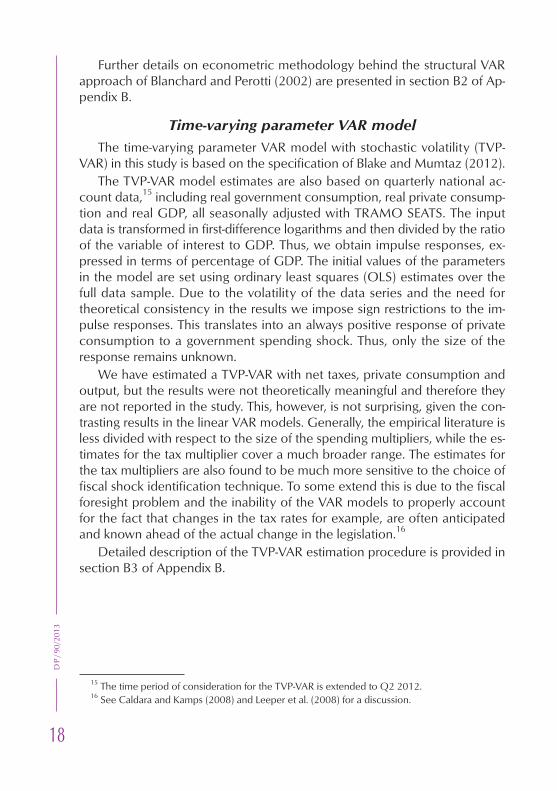
Despite the observed increase, however, the size of the spending mul-tiplier in Bulgaria remained as low as 0.4 at the peak of the financial crisis. Perhaps, the significant increase in the level of domestic savings during the crisis, induced mainly as a result of precautionary incentives, has been a rel-evant factor for limiting the increase in the multiplier’s size (Figure 8).

29

DIS

CU

SS

ION

PA

PE

RS

Figure 8HOUSEHOLD PROPENSITY TO SAVE

Sources: NSI Household Budget Survey, BNBNote: LHS – Quarterly change, seasonally adjusted data, available since 2004; RHS – Share of

disposable income, average per household member, seasonally adjusted data.

In the period 2010 – 2011 economic growth stabilized, imports recov-ered to their pre-crisis levels and public financing sustainability concerns were largely mitigated. Companies managed to improve the utilization of the excess capacities by redirecting the production towards the external market. These developments and the continuous growth of domestic savings have probably been relevant factors for the decline of the fiscal multiplier back to levels as low as 0.2.

Overall, the TVP-VAR model results reveal important information about the changes in the output effects of government consumption shocks in Bul-garia over the last fifteen years. It appears that the effectiveness of spending shocks in stimulating economic activity varies over time according to the underlying state of the economy. This relationship is found to be valid in a number of recent empirical studies, which analyse the links between fiscal multipliers and the state of the economy.23

23 Baum et al. (2012) provide a summary of results from selected studies on fiscal multipliers that employ non-linear approaches.

30

DP

/90/

2013

Conclusions, policy implications and further workThis paper analyses the impact of fiscal policy on real economic activity

in Bulgaria and provides a range of estimates for the tax and spending multi-pliers. We compare the results from linear structural VAR models with recur-sive identification and structural identification following Blanchard and Per-otti (2002) to the estimates from a time-varying parameters Bayesian SVAR, with the aim of investigating changes in the effectiveness of fiscal shocks in Bulgaria over the period 1999 – 2011.

The results of the linear VAR models indicate that the effectiveness of fis-cal policy in stimulating economic activity is generally low as first-year spend-ing multipliers do not exceed 0.4. The results regarding the tax multiplies are subject to a lot of uncertainty, as seen by the contrasting results in the esti-mated VAR models with different identification techniques, but the overall effect of tax measures on economic activity appears to be small and short-lived. These findings are in line with most of the studies on the catching-up EU Member State and support the general view that fiscal multipliers are usually small in small open economies.

The results of the two linear VAR models are broadly confirmed by the output of the TVP-VAR model, both pointing to a very limited effect of gov-ernment spending shocks on economic activity. However, TVP-VAR model reveals important information regarding the variations of the government consumption multiplier over time. Since the beginning of the sample (1999) the size of the first-year spending multiplier has been gradually decreasing from levels of around 0.3, down to a level of nearly 0.15 in 2007. As the global financial crisis started, the size of the multiplier doubled in less than two years, before decreasing again back to its pre-crisis levels, along with the economic recovery period (2010-2011). These results indicate that the underlying state of the economy appears to be a relevant factor for the non-linear effects of fiscal policy on economic growth in Bulgaria, even though further research is needed to support this view.

In terms of policy implications, the results imply that the effect of discre-tionary fiscal expansion on real economic activity in Bulgaria seems to be relatively small and short-lived, even during times of economic downturn. Analogously, if required, fiscal contractions are not expected to weigh heav-ily on economic activity, even in the short-run. Therefore, it is reasonable for the size of the fiscal multipliers to be taken into consideration when policy makers design fiscal consolidation or expansionary strategies. Even though the appropriate pace and effectiveness of a fiscal adjustment depends on a number of other factors, the small size of the fiscal multipliers in Bulgaria

31

DIS

CU

SS

ION

PA

PE

RS

imply that frontloaded consolidation would be in most cases preferable than back-loading the adjustment process, given the limited effects on output and the favourable impact on government debt dynamics, interest payments and fiscal sustainability. Back-loading the required fiscal consolidation effort is often motivated by the anticipation of lower multipliers in the future, associ-ated with improvement in the economic outlook. Such a strategy, however, entails certain risks, as fiscal multipliers are unobservable variable and there is a lot of uncertainty about their magnitude. This uncertainty is even further amplified given that the assessment of the multipliers’ size is based on fore-casts. In addition, back-loading fiscal adjustment requires much larger cumu-lative consolidation effort in the medium term, which in turn leads to a high level of public debt and correspondingly higher interest expenditure. In ad-dition, the postponement of the consolidation process is usually associated with a significant implementation risks related to the uncertainties about the materialization of the expected economic recovery as well as larger political risks associated with the postponement of the consolidation measures for the next election cycle.

The results are rather inconclusive in regards to the composition of the preferred consolidation strategy, but at least on impact it appears that ex-penditure restraints would have less negative effect on growth than increase in taxes. Nevertheless, more research is needed to understand the size of the multipliers of the different subcomponents of government expenditure and their dependence of the state of the economy. It plausible to assume that dis-cretionary increase or decrease in certain expenditure items might have larg-er output effects than others. Extending the research in this direction would provide valuable information about the preferable budget composition over the economic cycle. In addition, exploring the factors behind the dynamics of the fiscal multiplier over time is a natural subsequent step in researching the functioning of the fiscal transmission mechanism in Bulgaria. For these purposes, evaluations based on structural models, such as DSGE models, could provide a valuable input. Data constraints and the significant structural changes in the Bulgarian economy during the last fifteen years are other rel-evant arguments for further research based on structural model evaluations.

Nevertheless, the findings in this study have important policy implications for the desired fiscal policy over the cycle in the case of Bulgaria. Overall, the results of the empirical models suggest that there is little to gain in terms of economic output from active fiscal policy, even during periods of economic downturn.

In view of the small size of the fiscal multipliers and the limited scope of the monetary policy in Bulgaria to support economic growth, the fiscal

32

DP

/90/

2013

policy makers should concentrate on enhancing the quality of the govern-ment expenditure structure. Therefore, the fiscal adjustment strategies in the future should be based on cuts in inefficient public expenditure and coupled with the implementation of structural reforms in the ineffective public entities and loss-making state-owned companies, while preserving or even fostering growth-enhancing spending items. Heightening the role of the cost-benefit analysis as an analytical tool for weighing the benefits against the costs of certain legislative or regulatory proposals and larger public investment pro-jects could also increase the efficiency of public spending and the positive effects on economic output.

33

DIS

CU

SS

ION

PA

PE

RS

ReferencesAlfonso, A. and R. M. Sousa (2009), ‘The Macroeconomic Effects of

Fiscal Policy in Portugal: a Bayesian SVAR Analysis’, NIPE WP3/2009. Univer-sidade do Minho.

Alfonso, A. and R. M. Sousa (2009), ‘The Macroeconomic Effects of Fis-cal Policy’, ECB Working Paper Series No. 991

Auerbach Alan. J., and Yuriy Gorodnichenko, (2010), ‘Fiscal Multipliers in Recession and Expansion’, NBER Working Papers 17447.

Auerbach, Alan, J. and Yuriy Gorodnichenko, (2011), ‘Measuring the Output Responses to Fiscal Policy’, forthcoming in American Economic Jour-nal: Economic Policy.

Baum, A. and Koester, G. (2011), ‘The impact of fiscal policy on eco-nomic activity over the business cycle – evidence from a threshold VAR analysis’, Deutsche Bundesbank Discussion paper No. 03.2011

Baum A., Poplawski-Ribeiro M., and Weber A. (2012), ‘Fiscal Multipliers and the State of the Economy’, IMF Working Paper, WP/12/286

Benčík, M. (2009), ‘The Analysis of the Effects of Fiscal Policy on Busi-ness Cycle – A SVAR Application’, NBS Working Paper 2/2009. Národná Banka Slovenska.

Blake A. and Mumtaz H. (2012), ‘CCBS Technical Handbook – No.4 Ap-plied Bayesian econometrics for central bankers’, Centre for Central Banking Studies, Bank of England, September 2012

Blanchard, O. and Leigh D. (2013), ‘Growth Forecast Errors and Fiscal Multipliers’, IMF Working Paper, WP/13/1

Blanchard, O. and Quah, D. (1989), ‘The Dynamic effects of aggregate Demand and Supply Disturbances’, The American economic review , Vol 79, 1989, No.4, pp. 655-673

Blanchard, O. and Perotti R. (2002), ‘An Empirical Characterization of the Dynamic Effects of Changes in Government Spending and Taxes on Out-put’, Quarterly Journal of Economics, No. 117, pp. 1329-68.

Born, B., Juessen, F., Müller, G. J. (2012) ‘Exchange rate regimes and fiscal multipliers’, Journal of Economic Dynamics and Control, Volume 37, Issue 2, February 2013, Pages 446–465

Boussard, Jocelyn, Francisco de Castro and Matteo Salto (2012), ‘Fiscal Multipliers and Public Debt Dynamics in Consolidations’, European Econo-my Economic Papers 460 | July 2012

Burriel P., F. de Castro, D. Garrote, E. Gordo, J. Paredes and J. J. Perez (2009), ‘Fiscal policy shocks in the euro area and the US: an empirical as-sessment’, Working Paper No. 1133, European Central Bank.

34

DP

/90/

2013

Caldara, D. and C. Kamps (2008), ‘What Are the Effects of Fiscal Policy Shocks? A VAR-based Comparative Analysis’, ECB, Working Paper, No. 877, March.

Caprioli, F. and Momigliano, S. (2011), ‘The effects of Fiscal Shocks with Debt-Stabilizing Budgetary Policies in Italy’, Bank of Italy Working Paper No. 839

Castro F. and Hernández de Cos P., (2006), ‘The economic effects of ex-ogenous fiscal shocks in Spain: a SVAR approach’, Working paper No. 647, European Central Bank.

Coenen G., Erceg C., Freedman C., Furceri D., Kumhof M., Lalonde, R., Laxton D., Linde J., Mourougane A., Muir D., Mursula S., Roberts J., Roeger W., Resende C., Snudden S., Trabandt M. and Veld J., (2012), ‘Ef-fects of Fiscal Stimulus in Structural Models’, American Economic Journal: Macroeconomics 2012, 4 (1): 22–68.

Corsetti G., Kuester K., and Muller G. J., (2011), ‘Pegs, floats and the transmission of fiscal policy’, CEPR Discussion paper 8180

Cuaresma J., Eller M. and Mehrotra A., (2011), ‘The Economic Transmis-sion of Fiscal Policy Shocks from Western to Eastern Europe’, OeNB’s Focus on European Economic Integration (FEEI) 2/2011

Fatás, A., and I. Mihov (2001), ‘The Effects of Fiscal Policy on Consump-tion and Employment: Theory and Evidence’, CEPR Discussion Paper 2760. London.

Galí, J., J. D. López-Salido, and J. Vallés (2007), ‘Understanding the Ef-fects of Government Spending on Consumption,’ Journal of the European Economic Association, 5, 227–270

Giavazzi F. and M. Pagano (1990), ‘Can Severe Fiscal Contractions be Expansionary: Tales of Two Small European Countries’, NBER Macroeconom-ics Annual, 75-122.

Giordano, R., S. Momigliano, S. Neri and R. Perotti (2007), ‘The Effects of Fiscal Policy in Italy: Evidence from a VAR Model’, European Journal of Political Economy, No. 23, pp. 707-33.

Giorno C., P. Richardson, D. Roseveare and P. van den Noord, (1995),‘Potential output, output gaps and structural budget balances’, OECD Eco-nomic Studies No. 24, 1995/1.

Giuliodori M. and R. Beetsma (2004), ‘What are the spill-overs from fiscal shocks in Europe? An empirical analysis’,. Working Paper No. 325. Eu-ropean Central Bank.

Ilzetzki E., Mendoza E. G. and C. A. Vegh (2010), ‘How Big (Small?) are Fiscal Multipliers?’, NBER Working Paper No. 16479.

35

DIS

CU

SS

ION

PA

PE

RS

International Monetary Fund, 2012b, World Economic Outlook: Coping with High Debt and Sluggish Growth (Washington: International Monetary Fund, October).

Jemec, N. Kastelec, A. Delakorda, A. (2011), ‘How do fiscal shocks af-fect the macroeconomic dynamics in the Slovenian economy’, Working Pa-per No. 2/2011. Bank of Slovenia

Kirchner, M., J. Cimadomo, and S. Hauptmeier (2010), ‘Transmission of fiscal shocks in the euro area: time variation and driving forces’, Research Paper 21/2, Tinbergen Institute

Leeper E. M., N. Traum, and T.B. Walker (2011). ‘Clearing up the fiscal multiplier morass.’ NBER Working Paper 17444.

Leeper, E. M. (2010), ‘Monetary Science, Fiscal Alchemy,’ NBER Working Paper 16510

Leeper, E. M., T.B. Walker and S.S. Yang (2008). ‘Fiscal foresight: analyt-ics and econometrics.’ NBER Working Paper 14028.

Lendvai, J. (2007), ‘The Impact of Fiscal Policy in Hungary’, European Commission, Directorate General for Economic and Financial Affairs. Coun-try Focus IV(11). November.

Mançellari, A. (2011), ‘Macroeconomic effects of fiscal policy in Albania: a SVAR approach’, Bank of Albania Working Paper 5/2011

Mirdala, Rajmund (2009), ‘Effects of Fiscal Policy Shocks in the European Transition Economies’, Journal of Applied Research in Finance, Vol. 1, No. 2 (2009): pp. 141-155.

Mountford, A. and H. Uhlig (2009), ‘What are the effects of fiscal poli-cy shocks?’, Journal of Applied Econometrics, John Wiley & Sons, Ltd., vol. 24(6), pages 960-992.

Mountford, A. and H. Uhlig (2005), ‘What Are the Effects of Fiscal Policy Shocks?’, A SFB 649 Discussion Paper 2005-039. Humboldt University, Berlin.

Muir D., and Weber A., (2013), ‘Fiscal Multipliers in Bulgaria: Low But Still Relevant’, IMF Working Paper WP/13/49, February 2013

Nickel, C. and Tudyka, A. (2013), ‘Fiscal Stimulus in times of high debt. Reconsidering multipliers and twin deficits’, ECB Working Paper Series No 1513, February 2013)

Parker, J. (2011). ‘On Measuring the Effects of Fiscal Policy in Reces-sions,’ Journal of Economic Literature, American Economic Association, vol. 49 (3), pages 703-18, September

Pereira, M. and Lopes, A. (2010), ‘Time varying fiscal policy in the U.S’, Working Papers 201021, Banco de Portugal, Economics and Research De-partment.

36

DP

/90/

2013

Perotti, R. (1999): ‘Fiscal Policy in Good Times and Bad’, Quarterly Jour-nal of Economics, 138, 1399–1435.

Perotti, R. (2005), ‘Estimating the Effects of Fiscal Policy in OECD Coun-tries’, CEPR Discussion Paper 168, Center for Economic Policy Research, London.

Perotti, R. (2007), ‘In Search of the Transmission Mechanism of Fiscal Policy’, NBER Working Paper No. 13143, NBER Macroeconomics Annual 2007, Volume 22 (2008), University of Chicago Press.

Ramey, V. A. (2007), ‘Identifying Government Spending Shocks: It’s All in the Timing’, University of California, San Diego.

Ramey, V. A., and M.D. Shapiro (1998), ‘Costly Capital Reallocation and the Effects of Government Spending’, Carnegie-Rochester Conference Series on Public Policy 48 (June): 145-194.

Romer, C. and D.H. Romer (2010), ‘The Macroeconomic Effects of Tax Changes: Estimates Based on a New Measure of Fiscal Shocks,’ American Economic Review, 100, 763-801.

Rzonca, A. and P. Cizkovicz (2005), ‘Non-Keynesian Effects of Fiscal Contraction in New Member States’, ECB Working Papers No.519. Septem-ber 2005.

Spilimbergo A., Symansky S. and Schindler M. (2009), ‘Fiscal Multipli-ers’, IMF Staff Position Note. SPN/09/11, International Monetary Fund.

Uhlig, H. (2005), ‘What Are the Effects of Monetary Policy on Output? Results from an Agnostic Identification Procedure’, Journal of Monetary Eco-nomics 52 (2): 381-419.

37

DIS

CU

SS

ION

PA

PE

RS

GD

P at

200

5 pr

ices

GD

P at

200

5 pr

ices

- Re

al G

over

n-m

ent C

onsu

mpt

ion

-Rea

l Gov

ernm

ent

Inve

stm

ent (

defla

ted

with

the

inve

stm

ent

defla

tor)

Fina

l Con

sum

ptio

n of

Hou

seho

lds

and

NPI

SH’s

at 2

005

pric

es

Gro

ss F

ixed

Cap

ital F

orm

atio

n at

200

5 pr

ices

Gov

ernm

ent C

onsu

mpt

ion

at 2

005

pric

es

Out

put

Y

Priv

ate

outp

ut

YPR

Con

sum

ptio

n C

ON

Inve

stm

ent

INV

Gov

ernm

ent

GC

Con

sum

ptio

n

log

mill

ions

of

dom

estic

cu

rren

cy

log

mill

ions

of

dom

estic

cu

rren

cy

log

mill

ions

of

dom

estic

cu

rren

cy

log

mill

ions

of

dom

estic

cu

rren

cy

log

mill

ions

of

dom

estic

cu

rren

cy

Seas

onal

ad

just

men

t

Seas

onal

ad

just

men

t

Seas

onal

ad

just

men

t

Seas

onal

ad

just

men

t

Seas

onal

ad

just

men

t

Nat

iona

l Sta

tistic

al In

sti-

tute

- N

atio

nal A

ccou

nts

data

Nat

iona

l Sta

tistic

al In

sti-

tute

- N

atio

nal A

ccou

nts

data

and

Qua

rter

ly N

on-

Fina

ncia

l Acc

ount

s of

the

Gen

eral

Gov

enm

ent

Nat

iona

l Sta

tistic

al -

Inst

i-tu

te N

atio

nal A

ccou

nts

data

Nat

iona

l Sta

tistic

al In

sti-

tute

- N

atio

nal A

ccou

nts

data

Nat

iona

l Sta

tistic

al In

sti-

tute

- N

atio

nal A

ccou

nts

data

Appe

ndix

A. D

etai

ls on

dat

a

Va

riab

les

Cod

e D

escr

iptio

n an

d ca

lcul

atio

n U

nit

Trea

tmen

t So

urce

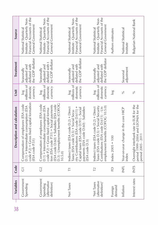
38

DP

/90/

2013

Com

pens

atio

n of

em

ploy

ees

(ESA

cod

e D

.1) +

Inte

rmed

iate

con

sum

ptio

n (E

SA

code

P.2

) + G

ross

fixe

d ca

pita

l for

mat

ion

(ESA

cod

e P.

51)

Com

pens

atio

n of

em

ploy

ees

(ESA

cod

e D

.1) +

Inte

rmed

iate

con

sum

ptio

n (E

SA

code

P.2

) + G

ross

fixe

d ca

pita

l for

ma-

tion

(ESA

cod

e P.

51) +

Soc

ial p

aym

ents

(E

SA c

ode

D.6

0) +

Sub

sidi

es (E

SA c

ode

D.3

) - U

nem

ploy

men

t ben

efits

(CO

FOG

10

.5.0

)

Indi

rect

taxe

s (E

SA c

ode

D.2

) + D

irect

Ta

xes

(ESA

cod

e D

.5) +

Soc

ial S

ecu-

rity

Con

trib

utio

ns (E

SA c

ode

D.6

11) +

C

apita

l tax

es (E

SA c

ode

D.9

1) -

Soci

al

paym

ents

(ESA

cod

e D

.60)

- Su

bsid

ies

(ESA

cod

e D

.3)

Indi

rect

taxe

s (E

SA c

ode

D.2

) + D

irect

Ta

xes

(ESA

cod

e D

.5) +

Soc

ial S

ecur

ity

Con

trib

utio

ns (E

SA c

ode

D.6

11)

- Un-

empl

oym

ent b

enef

its (C

OFO

G 1

0.5.

0)

Inde

x 20

05 =

100

Year

-on-

year

cha

nge

in th

e co

re H

ICP

inde

x

Ove

rnig

ht in

terb

ank

rate

in E

UR

for t

he

perio

d 19

99 -2

004

and

LEO

NIA

for t

he

perio

d 20

05 -

2011

Gov

ernm

ent

G1

Spen

ding

Gov

ernm

ent

G2

Spen

ding

(a

ltern

ativ

e de

finiti

on)

Net

Tax

es

T1

‘Net

Tax

es

T2(a

ltern

ativ

e de

finiti

on)’

Fore

ign

FD

dem

and

Infla

tion

INFL

Inte

rest

rate

s IN

TS

log

mill

ions

of

dom

estic

cu

rren

cy

log

mill

ions

of

dom

estic

cu

rren

cy

log

mill

ions

of

dom

estic

cu

rren

cy

log

mill

ions

of

dom

estic

cu

rren

cy

log % %

Seas

onal

ly

adju

sted

and

de

flate

d w

ith

the

GD

P de

flato

r

Seas

onal

ly

adju

sted

and

de

flate

d w

ith t

he G

DP

defla

tor

Seas

onal

ly

adju

sted

and

de

flate

d w

ith

the

GD

P de

flato

r

Seas

onal

ly

adju

sted

and

de

flate

d w

ith

the

GD

P de

flato

r

Seas

onal

ad

just

men

t

Nat

iona

l Sta

tistic

al

Inst

itute

- Q

uart

erly

Non

-Fi

nanc

ial A

ccou

nts

of th

e G

ener

al G

oven

men

t

Nat

iona

l Sta

tistic

al

Inst

itute

- Q

uart

erly

Non

-Fi

nanc

ial A

ccou

nts

of th

e G

ener

al G

oven

men

t

Nat

iona

l Sta

tistic

al

Inst

itute

- Q

uart

erly

Non

-Fi

nanc

ial A

ccou

nts

of th

e G

ener

al G

oven

men

t

Nat

iona

l Sta

tistic

al

Inst

itute

- Q

uart

erly

Non

-Fi

nanc

ial A

ccou

nts

of th

e G

ener

al G

oven

men

t

Aut

hors

est

imat

es

Nat

iona

l Sta

tistic

al

Inst

itute

Bulg

aria

n N

atio

nal B

ank

Va

riab

les

Cod

e D

escr

iptio

n an

d ca

lcul

atio

n U

nit

Trea

tmen

t So

urce

39

DIS

CU

SS

ION

PA

PE

RS

Appendix B. Details on the econometric methodologyB.1. The recursive approachThe baseline VAR model in our study includes three endogenous varia-

bles in real terms: government spending (g), GDP (y) and net taxes (). Apart from the endogenous variables, we also include a constant (), a linear time trend (t) and the log-transformed foreign demand (fd) for Bulgarian exports as exogenous variables.

The reduced-form VAR model can be expressed in the following way:

Xt = μ0 + μ1t + μ2 fdt + A(L) Xt −1 + ut , (1)

where Xt = [gt yt t] is a three-dimensional vector of endogenous variables, A(L) is a 4th-order lag polynomial and ut is a vector of residuals (innovations). As in Blanchard and Perotti (2002) we choose a lag length of four quarters in order to ensure serially uncorrelated residuals.24 The inclusion of four lags is a common practice in the estimation of models with quarterly data (Caldara and Kamps, 2008).

Notice that in the first extended (4-variable) recursive VAR, the vector of variables would be augmented to: Xt = [gt yt cont /invt], where cont /invt indicates either private consumption or investment. In the second extension of the recursive VAR (5-variable), the vector becomes: Xt = [gt yt t t intrst], where t is inflation and intrst is short-term interest rates.

In order to recover the structural shocks that affect the endogenous vari-ables of the model we use the recursive identification approach, which is based on Cholesky decomposition of the variance-covariance matrix of the model residuals. As the reduced form residuals ut are usually contemporane-ously correlated, it is necessary to transform them into structural shocks. For the purpose we multiply equation (1) by the matrix A0, which is a diagonal one. Thus, the new (structural) shocks et = A0ut are no longer correlated and they can be economically interpreted. The resulting equation is the following:

A0Xt = A0 + A0t + A0fdt + A0A(L)Xt-1 + Bet (2)The equation A0ut = Bet gives us the relation between the reduced-form

residuals (ut), which we observe and the structural shocks (et), which we want to identify.

In order to identify the structural model, the parameters in A0 and B have to be restricted. In the recursive identification approach, the Cholesky de-

24 Formal tests as the Akaike information criterion (AIC) and other information criteria (FPE, HQ, SC suggest the inclusion of two lags.

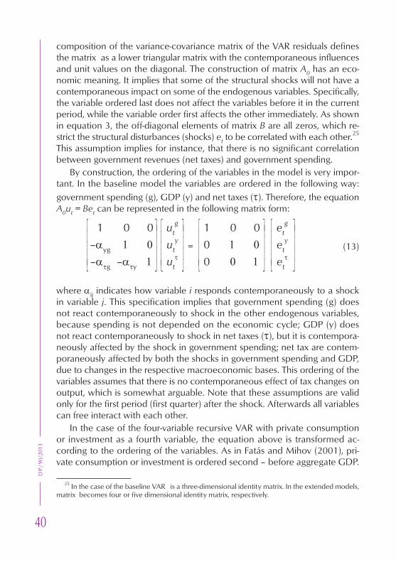
40

DP

/90/

2013

composition of the variance-covariance matrix of the VAR residuals defines the matrix as a lower triangular matrix with the contemporaneous influences and unit values on the diagonal. The construction of matrix A0 has an eco-nomic meaning. It implies that some of the structural shocks will not have a contemporaneous impact on some of the endogenous variables. Specifically, the variable ordered last does not affect the variables before it in the current period, while the variable order first affects the other immediately. As shown in equation 3, the off-diagonal elements of matrix B are all zeros, which re-strict the structural disturbances (shocks) et to be correlated with each other.25

This assumption implies for instance, that there is no significant correlation between government revenues (net taxes) and government spending.

By construction, the ordering of the variables in the model is very impor-tant. In the baseline model the variables are ordered in the following way: government spending (g), GDP (y) and net taxes (). Therefore, the equation A0ut = Bet can be represented in the following matrix form:

= (13)

where ij indicates how variable i responds contemporaneously to a shock in variable j. This specification implies that government spending (g) does not react contemporaneously to shock in the other endogenous variables, because spending is not depended on the economic cycle; GDP (y) does not react contemporaneously to shock in net taxes (), but it is contempora-neously affected by the shock in government spending; net tax are contem-poraneously affected by both the shocks in government spending and GDP, due to changes in the respective macroeconomic bases. This ordering of the variables assumes that there is no contemporaneous effect of tax changes on output, which is somewhat arguable. Note that these assumptions are valid only for the first period (first quarter) after the shock. Afterwards all variables can free interact with each other.

In the case of the four-variable recursive VAR with private consumption or investment as a fourth variable, the equation above is transformed ac-cording to the ordering of the variables. As in Fatás and Mihov (2001), pri-vate consumption or investment is ordered second – before aggregate GDP.

25 In the case of the baseline VAR is a three-dimensional identity matrix. In the extended models, matrix becomes four or five dimensional identity matrix, respectively.

1 0 0 –yg –g –y

1 0 0 0 0

utg

uty

ut

etg

ety

et

41

DIS

CU

SS

ION

PA

PE

RS

Thus, the equation A0ut = Bet would consist of four by four matrices and four-variable vectors.

In the second extended VAR model with five variables - government spending, GDP, inflation, net taxes and interest rates, the equation would be represented in the following form:

=

The ordering of the variables is the same as in Fatás and Mihov (2001), namely, government spending (g), GDP (y), inflation (), net taxes () and interest rates (r). The implications of the ordering and the associated eco-nomic interpretation are discussed in Fatás and Mihov (2001) and Caldara and Kamps (2008).

B.2. The approach of Blanchard and Perotti In the application of the approach of Blanchard and Perotti (2002) we

start again from the reduced form VAR specification from equation (1),

Xt = μ0 + μ1t + μ2 fdt + A(L) Xt −1 + ut ,where Xt = [t gt yt] is a three-dimensional vector of endogenous variables, which includes net taxes, government spending and output. Again, as in the recursive identification approach, we need to identify matrices A0 and B, which provide the relation between the reduced-form residuals ut and the structural disturbances et : A0ut = Bet. We follow a four step approach as in Jemec et al. (2011) and Gordano et al. (2007). First, after the reduced form VAR model is estimated, we decompose the reduced-form residuals of taxes ut ut and government spending ut

g in the following way: ut

= yuty + get

g + et(4)

ut g = gyut

y + gt et+ et

g (5)

The coefficients y and gy are elements of the matrix A0 and represent the response (both automatic and discretionary) of taxes and government spending to a shock in the economic activity. The coefficients g and gt capture how the structural shock in government spending affects contempo-raneously taxes and vice versa.

1 0 0 0 0 –yg –g–y –g–y– –rg –ry –r –r

1 0 0 0 0 0 0 0 0

etg

ety

et

et

etr

utg

uty

ut

ut

utr

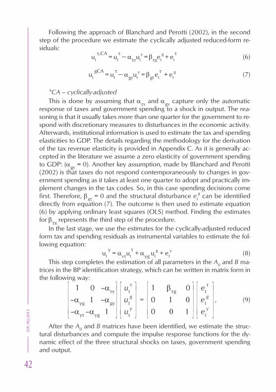
42

DP

/90/

2013

Following the approach of Blanchard and Perotti (2002), in the second step of the procedure we estimate the cyclically adjusted reduced-form re-siduals:

ut CA = ut

yuty = get

g + et(6)

ut gCA = ut

gyuty = gt et

+ etg (7)

*CA – cyclically-adjustedThis is done by assuming that y and gy capture only the automatic

response of taxes and government spending to a shock in output. The rea-soning is that it usually takes more than one quarter for the government to re-spond with discretionary measures to disturbances in the economic activity. Afterwards, institutional information is used to estimate the tax and spending elasticities to GDP. The details regarding the methodology for the derivation of the tax revenue elasticity is provided in Appendix C. As it is generally ac-cepted in the literature we assume a zero elasticity of government spending to GDP: (gy = 0). Another key assumption, made by Blanchard and Perotti (2002) is that taxes do not respond contemporaneously to changes in gov-ernment spending as it takes at least one quarter to adopt and practically im-plement changes in the tax codes. So, in this case spending decisions come first. Therefore, g = 0 and the structural disturbance et

g can be identified directly from equation (7). The outcome is then used to estimate equation (6) by applying ordinary least squares (OLS) method. Finding the estimates for g represents the third step of the procedure.

In the last stage, we use the estimates for the cyclically-adjusted reduced form tax and spending residuals as instrumental variables to estimate the fol-lowing equation:

ut y = yut

+ yg utg+ et

y (8)This step completes the estimation of all parameters in the A0 and B ma-

trices in the BP identification strategy, which can be written in matrix form in the following way:

= , (9)

After the A0 and B matrices have been identified, we estimate the struc-tural disturbances and compute the impulse response functions for the dy-namic effect of the three structural shocks on taxes, government spending and output.

1 0 –y

–yg –gy

–y–yg

1 g 0 0 0

ut

utg

uty

et

etg

ety

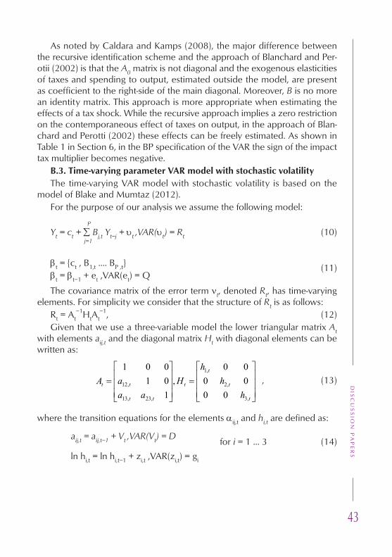
43

DIS

CU

SS

ION

PA

PE

RS

As noted by Caldara and Kamps (2008), the major difference between the recursive identification scheme and the approach of Blanchard and Per-otii (2002) is that the A0 matrix is not diagonal and the exogenous elasticities of taxes and spending to output, estimated outside the model, are present as coefficient to the right-side of the main diagonal. Moreover, B is no more an identity matrix. This approach is more appropriate when estimating the effects of a tax shock. While the recursive approach implies a zero restriction on the contemporaneous effect of taxes on output, in the approach of Blan-chard and Perotti (2002) these effects can be freely estimated. As shown in Table 1 in Section 6, in the BP specification of the VAR the sign of the impact tax multiplier becomes negative.

B.3. Time-varying parameter VAR model with stochastic volatilityThe time-varying VAR model with stochastic volatility is based on the

model of Blake and Mumtaz (2012). For the purpose of our analysis we assume the following model:

PYt = ct + Bj,t Yt−j + t ,VAR(t) = Rt (10) j=1

t = {ct , B1,t .... BP ,t}t = t−1 + et ,VAR(et) = Q

(11)

The covariance matrix of the error term t, denoted Rt, has time-varying elements. For simplicity we consider that the structure of Rt is as follows:

Rt = At−1HtAt

−1, (12)Given that we use a three-variable model the lower triangular matrix At

with elements aij,t and the diagonal matrix Ht with diagonal elements can be written as:

, (13)

where the transition equations for the elements ij,t and hi,t are defined as:

aij,t = aij,t−1 + Vt ,VAR(Vt) = D for i = 1 ... 3 (14) ln hi,t = ln hi,t−1 + zi,t ,VAR(zi,t) = gi

44

DP

/90/

2013

Appendix C. Details on the derivation of tax revenue elasticityIn line with the OECD approach, the net tax elasticity is a weighted aver-

age of the elasticities of four tax categories (personal income tax, corporate income tax, indirect taxes and social security contributions) and net transfers (taken with a minus sign). More formally:

where i is the elasticity of tax category i to the respective macro tax base,

i,y is the elasticity of the tax base to GDP and is the share of respective

tax category in the tax aggregate. The latter variable is positive for the four tax categories and negative for net transfers (unemployment benefits in the alternative specification). The elasticities of the various categories to the re-spective tax bases are calibrated on the basis of the tax legislation and are summarized in Table C1. For all categories, the elasticity is equal or close to 1 as the Bulgarian tax system is proportional with flat direct tax rates. It should be mentioned that for personal income tax we assume a higher elas-ticity until 2008, when the tax was progressive and afterwards when a flat tax rate with no minimum non-taxable income was introduced. Since only data for aggregate direct taxes is available at the quarterly frequency, we have used quarterly cash-data profiles to interpolate the annual data for personal income tax and other direct taxes. Corporate income tax receivables are estimated as a residual variable.

Table C1BUDGETARY ELASTICITIES RELATIVE TO CORRESPONDING

MACROECONOMIC BASES

Budget item Macroeconomic base Budgetary elasticity

Direct taxes on households Average compensation per employee 1.2 up to 2007,

1.0 afterwards

Employment 1.0

Social security contributions Average compensation per employee 1.0

Employment 1.0

Direct taxes on companies Operating surplus 1.05

Indirect taxes Private consumption 1.0

Net transfers GDP -0.2

iyiy ii ,

i

45

DIS

CU

SS

ION

PA

PE

RS

The elasticity of different tax bases with respect to output has been evalu-ated econometrically by using error-correction specifications. The next table summarizes these elasticities together with the information on the average share of the different tax categories in aggregate net taxes.

Table C2

DERIVATION OF THE NET TAX ELASTICITY

Elasticity with Average share in net Weighted

respect to GDP taxes 1999-2011 elasticity

Corporate income tax 0.82 0.17 0.14

Personal income tax* 0.27 0.20 0.05

Indirect taxes 1.03 0.92 0.95

Social Security Contributions 0.27 0.55 0.15

Elasticity of tax revenues 1.29

Net transfers -0.2 0.85 -0.17

Elasticity net taxes 1.12

Our estimate is somewhat lower than the average elasticity, estimated by Burriel et al (2009) for the EU (1.54) and slightly higher than the one, estimat-ed by Jemec and Delakorda (2011) for Slovenia (0.87). If we apply the alter-native definition for net taxes (current taxes minus unemployment benefits), applied by Baum and Koester (2011), our elasticity estimate is 0.87, which is also lower than the identical estimate for Germany (1.02). However, what we observe from the data is that the net tax elasticity is changing over time (Figure C1). This can be attributed to the impact of the economic cycle as well as to the gradual movement from a more progressive to a more propor-tional tax system and to the constantly increasing share of indirect taxes. The time-variation of the tax elasticity is another argument to take an advantage of a time-varying parameter VAR model.

46

DP

/90/

2013

Figure C1TIME VARYING ELASTICITY OF NET TAXES

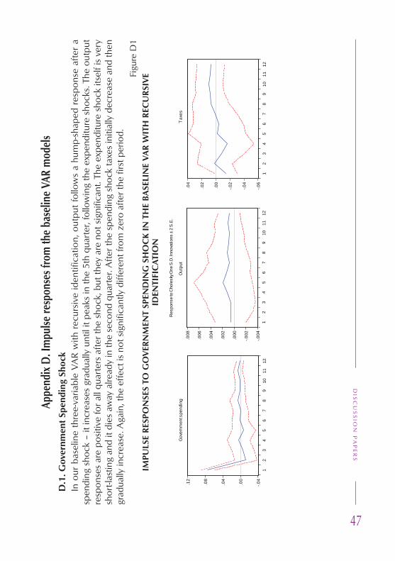
47

DIS

CU

SS

ION

PA

PE

RS

-.04

.00

.04

.08

.12

12

34

56

78

910

1112

-.004

-.002

.000

.002

.004

.006

.008

12

34

56

78

910

1112

Res

pons

e to

Cho

lesk

y One

S.D

. Inn

ovat

ions

± 2

S.E

.

-.06

-.04

-.02

.00

.02

.04

12

34

56

78

910

1112

Out

put

Gov

ernm

ent s

pend

ing

Tax

es

Appe

ndix

D. I

mpu

lse re

spon

ses f

rom

the

base

line

VAR

mod

els

D.1

. Gov

ernm

ent S

pend

ing

Shoc

kIn

our

bas

elin

e th

ree-

varia

ble

VAR

with

rec

ursi

ve id

entif

icat

ion,

out

put

follo

ws

a hu

mp-

shap

ed r

espo

nse

afte

r a

spen

ding

sho

ck –

it in

crea

ses

grad

ually

unt

il it

peak

s in

the

5th

quar

ter,

follo

win

g th

e ex

pend

iture

sho

cks.

The

out

put

resp

onse

s ar

e po

sitiv

e fo

r all

quar

ters

afte

r the

sho

ck, b

ut th

ey a

re n

ot s

igni

fican

t. Th

e ex

pend

iture

sho

ck it

self

is v

ery

shor

t-las

ting

and

it di

es a

way

alre

ady

in th

e se

cond

qua

rter

. Afte

r the

spe

ndin

g sh

ock

taxe

s in

itial

ly d

ecre

ase

and

then

gr

adua

lly in

crea

se. A

gain

, the

effe

ct is

not

sig

nific

antly

diff

eren

t fro

m z

ero

afte

r the

firs

t per

iod.

Fi

gure

D1

IMPU

LSE

RES

PON

SES

TO G

OV

ERN

MEN

T SP

END

ING

SH

OC

K IN

TH

E BA

SELI

NE

VAR

WIT

H R

ECU

RSI

VE

IDEN

TIFI

CAT

ION

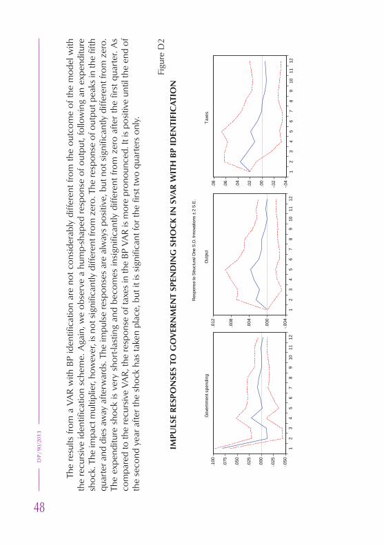
48

DP

/90/

2013

The

resu

lts fr

om a

VA

R w

ith B

P id

entif

icat

ion

are

not c

onsi

dera

bly

diffe

rent

from

the

outc

ome

of th

e m

odel

with

th

e re

curs

ive

iden

tific

atio

n sc

hem

e. A

gain

, we

obse

rve

a hu

mp-

shap

ed re

spon

se o

f out

put,

follo

win

g an

exp

endi

ture

sh

ock.

The

impa

ct m

ultip

lier,

how

ever

, is

not s

igni

fican

tly d

iffer

ent f

rom

zer

o. T

he re

spon

se o

f out

put p

eaks

in th

e fif

th

quar

ter a

nd d

ies

away

afte

rwar

ds. T

he im

pulse

resp

onse

s ar

e al

way

s po

sitiv

e, b

ut n

ot s

igni

fican

tly d

iffer

ent f

rom

zer

o.

The

expe

nditu

re s

hock

is v

ery

shor

t-las

ting

and

beco

mes

insi

gnifi

cant

ly d

iffer

ent f

rom

zer

o af

ter

the

first

qua

rter

. As

com

pare

d to

the

recu

rsiv

e VA

R, th

e re

spon

se o

f tax

es in

the

BP V

AR

is m

ore

pron

ounc

ed. I

t is

posi

tive

until

the

end

of

the

seco

nd y

ear a

fter t

he s

hock

has

take

n pl

ace,

but

it is

sig

nific

ant f

or th

e fir

st tw

o qu

arte

rs o

nly.

Figu

re D

2IM

PULS

E R

ESPO

NSE

S TO

GO

VER

NM

ENT

SPEN

DIN

G S

HO

CK

IN S

VAR

WIT

H B

P ID

ENTI

FIC

ATIO

N

-.04

-.02

.00

.02

.04

.06

.08

12

34

56

78

910

1112

-.050

-.025

.000

.025

.050

.075

.100

12

34

56

78

910

1112

Gov

ernm

ent s

pend

ing

-.004

.000

.004

.008

.012

12

34

56

78

910

1112

Res

pons

e to

Stru

ctur

al O

ne S

.D. I

nnov

atio

ns ±

2 S

.E.

Out

put

Tax

es

49

DIS

CU

SS

ION

PA

PE

RS

D.2

. Tax

Sho

ckTh

e ba

selin

e VA

R m

odel

pro

vide

s an

inte

rest

ing

resu

lt. T

he ta

x sh

ock

caus

es o

utpu

t to

initi

ally

incr

ease

for

eigh

t qu

arte

rs, b

efor

e its

res

pons

e tu

rns

nega

tive.

Aga

in, t

he im

pulse

res

pons

e is

not

sig

nific

antly

diff

eren

t fro

m z

ero

afte

r th

e se

cond

qua

rter

. Ove

rall,

sho

cks

in n

et t

axes

see

m to

be

mor

e pe

rsis

tent

as

com

pare

d to

spe

ndin

g sh

ocks

. The

du

ratio

n of

the

tax

shoc

k is

aro

und

two

year

s an

d th

e re

spon

se is

sig

nific

antly

pos

itive

for

the

first

four

qua

rter

s. F

ol-

low

ing

a ta

x in

crea

se, g

over

nmen

t spe

ndin

g do

es s

eem

to re

act p

ositi

vely

and

sub

stan

tially

. To

som

e ex

tent

this

is d

ue

to th

e re

stric

tions

impo

sed

by th

e re

curs

ive

spec

ifica

tion.

The

res

pons

e of

spe

ndin

g pe

aks

in th

e fo

urth

qua

rter

and

di

es a

way

afte

rwar

ds.

Figu

re D

3IM

PULS

E R

ESPO

NSE

S TO

GO

VER

NM

ENT

TAX

SHO

CK

IN T

HE

BASE

LIN

E VA

R W

ITH

REC

UR

SIV

E ID

ENTI

FIC

ATIO

N

-.04

-.02

.00

.02

.04

.06

12

34

56

78

910

1112

-.008

-.004

.000

.004

.008

12

34

56

78

910

1112

Resp

onse

to C

hole

sky

One

S.D

. Inn

ovat

ions

± 2

S.E

.

-.08

-.04

.00

.04

.08

.12

12

34

56

78

910

1112

Gove

rnm

ent s

pend

ing

Out

put

Taxe

s

50

DP

/90/

2013

In t

he V

AR

mod

el w

ith B

P id

entif

icat

ion,

the

sig

n of

the

impa

ct ta

x m

ultip

lier

chan

ges

and

the

effe

ct o

n ou

tput

, fo

llow

ing

a ta

x in

crea

se, b

ecom

es n

egat

ive

and

sign

ifica

nt. T

he o

utpu

t res

pons

e be

com

es in

sign

ifica

nt a

lread

y in

the

seco

nd q

uart

er, i

t rem

ains

pos

itive

for

thre

e qu

arte

rs b

efor

e it

turn

s ne

gativ

e. T

he re

spon

se o

f gov

ernm

ent s

pend

ing

afte

r a ta

x sh

ock

is v

ery

sim

ilar t

o th

e ba

selin

e m

odel

. It t

akes

thre

e qu

arte

rs b

efor

e go

vern

men

t exp

endi

ture

incr

ease

s fo

llow

ing

a ta

x in

crea

se a

nd th

e re

spon

se p

eaks

in th

e fif

th q

uart

er. A

fterw

ards

, the

res

pons

e slo

wly

die

s aw

ay. T

his

mod

el a

lso c

onfir

ms

the

fact

that

tax

shoc

ks a

re u

sual

ly m

ore

pers

isten

t tha

n sh

ocks

in g

over

nmen

t spe

ndin

g. Figu

re D

4IM

PULS

E R

ESPO

NSE

S TO

GO

VER

NM

ENT

TAX

SHO

CK

IN T

HE

VAR

WIT

H B

P ID

ENTI

FIC

ATIO

N

-.10

-.05

.00

.05

.10

12

34

56

78

910

1112

-.04

-.02

.00

.02

.04

.06

12

34

56

78

910

1112

-.008

-.004

.000

.004

.008

.012

12

34

56

78

910

1112

Resp

onse

to S

truct

ural

One

S.D

. Inn

ovat

ions

± 2

S.E

.

Gove

rnm

ent s

pend

ing

Out

put

Taxe

s

51

DIS

CU

SS

ION

PA

PE

RS

Appendix E. Robustness checkE.1. Effects on Private Consumption and InvestmentThe results from the extended recursive VAR model with private con-

sumption or investment as fourth variable show that the responses of the other endogenous variables do not change significantly after the tax or the spending shock. Private consumption reacts positively to a government spending shock in the first period and its response turns negative afterwards (Figure E1). The effect on investment is much stronger and always positive, but becomes significant in the 3rd quarter after the shock (Figure E2). Both consumption and investment react in a similar way to a tax shock with a tem-porary increase in the first two quarters. Overall, it appears that these results are more in support of the Real Business Cycle models, which predicts a drop in private consumption as a result of expansionary fiscal policy. Never-theless, the statistical significance of the results from the VAR model do not allow for any strong conclusions.

Figure E1IMPULSE RESPONSE OF CONSUMPTION AFTER GOVERNMENT

SPENDING AND A TAX SHOCK IN VAR WITH RECURSIVE IDENTIFICATION

-.015

-.010

-.005

.000

.005

.010

.015

1 2 3 4 5 6 7 8 9 10 11 12

Response of consumption after a spending shock

-.015

-.010

-.005

.000

.005

.010

.015

1 2 3 4 5 6 7 8 9 10 11 12

Response of consumption after a tax shock

Response to Cholesky One S.D. Innovations ± 2 S.E.

52

DP

/90/

2013

Figure E2IMPULSE RESPONSE OF INVESTMENT AFTER GOVERNMENT

SPENDING AND A TAX SHOCK IN VAR WITH RECURSIVE IDENTIFICATION

E.2. Alternative specification of government spending and net taxesTo check the robustness of the linear VAR model results as we opt for a

different classification of expenditures and net taxes. As stated in the data description section of the paper, there are strong arguments for including social payments on the expenditure side as these account for a substantial part of total government spending in Bulgaria and represent an important instrument for stimulating internal demand.

We estimate two separate models with an alternative specification of gov-ernment spending and net taxes - one five-variable VAR with recursive identi-fication scheme and one three-variable structural VAR with BP specification. In the case of the structural VAR, the use of the different net tax aggregate requires re-estimation of the net tax elasticity, which is somewhat lower with the alternative specification.

The outcome (Figures E3, E4, E5 and E6) shows that the effects of a spending and a tax shock on output are not considerably different as com-pared to the results of the baseline models. Regarding the recursive VAR, the only significant response that we observe in respect to inflation and interest rate is the impact rise of interest rates after a spending shock (Figure E3). In fact, the reduced VAR residuals are normally distributed only when the alter-native definition for government spending and net taxes is used.

-.04

-.02

.00

.02

.04

.06

.08

1 2 3 4 5 6 7 8 9 10 11 12

Response of investment after a spending shock

-.04

-.02

.00

.02

.04

.06

.08

1 2 3 4 5 6 7 8 9 10 11 12

Response of investment after a tax shock

Response to Cholesky One S.D. Innovations ± 2 S.E.

53

DIS

CU

SS

ION

PA

PE

RS

Figu

re E

3EX

TEN

DED

FIV

E-VA

RIA

BLE

VAR

WIT

H R

ECU

RSI

VE

IDEN

TIFI

CAT

ION

– R

ESPO

NSE

S A

FTER

GO

VER

NM

ENT

SPEN

DIN

G S

HO

CK

Figu

re E

4EX

TEN

DED

FIV

E-VA

RIA

BLE

VAR

WIT

H R

ECU

RSI

VE

IDEN

TIFI

CAT

ION

– R

ESPO

NSE

S A

FTER

GO

VER

NM

ENT

TAX

SHO

CK

54

DP

/90/

2013

Figu

re E

5SV

AR

WIT

H A

LTER

NAT

IVE

DEF

INIT

ION

OF

GO

VER

NM

ENT

SPEN

DIN

G A

ND

TA

XES

– R

ESPO

NSE

S A

FTER

G

OV

ERN

MEN

T TA

X SH

OC

K

Figu

re E

6SV

AR

WIT

H A

LTER

NAT

IVE

DEF

INIT

ION

OF

GO

VER

NM

ENT

SPEN

DIN

G A

ND

TA

XES

– R

ESPO

NSE

S A

FTER

G

OV

ERN

MEN

T SP

END

ING

SH

OC

K

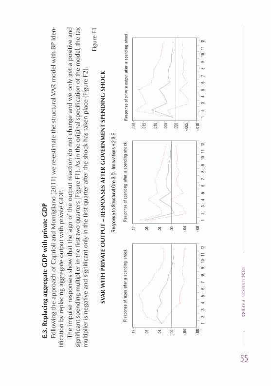
55

DIS

CU

SS

ION

PA

PE

RS

E.3.

Rep

laci

ng a

ggre

gate

GD

P w

ith p

riva

te G

DP

Follo

win

g th

e ap

proa

ch o

f Cap

rioli

and

Mom

iglia

no (2

011)

we

re-e

stim

ate

the

stru

ctur

al V

AR

mod

el w

ith B

P id

en-

tific

atio

n by

repl

acin

g ag

greg

ate

outp

ut w

ith p

rivat

e G

DP.

The

impu

lse

resp

onse

s sh

ow t

hat t

he s

ign

of t

he o

utpu

t rea

ctio

n do

not

cha

nge

and

we

only

get

a p

ositi

ve a

nd

sign

ifica

nt s

pend

ing

mul

tiplie

r in

the

first

two

quar

ters

(Fig

ure

F1).

As

in th

e or

igin

al s

peci

ficat

ion

of th

e m

odel

, the

tax

mul

tiplie

r is

nega

tive

and

sign

ifica

nt o

nly

in th

e fir

st q

uart

er a

fter t

he s

hock

has

take

n pl

ace

(Fig

ure

F2).

Figu

re F

1SV

AR

WIT

H P

RIV

ATE

OU

TPU

T –

RES

PON

SES

AFT

ER G

OV

ERN

MEN

T SP

END

ING

SH

OC

K

56

DP

/90/

2013

Figu

re F

2SV

AR

WIT

H P

RIV

ATE

OU

TPU

T –

RES

PON

SES

AFT

ER G

OV

ERN

MEN

T TA

X SH

OC

K

57

DIS

CU

SS

ION

PA

PE

RS

Appe

ndix

F. Su

pple

men

tary

figu

res a

nd ta

bles

Figu

re F

3ST

ABI

LITY

OF

VAR

SPE

CIF

ICAT

ION

Ba

selin

e 3-

varia

ble

VAR

5-va

riabl

e VA

R

VA

R w

ith p

rivat

e ou

tput

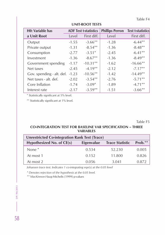
58

DP

/90/

2013

Table F4UNIT-ROOT TESTS

H0: Variable has ADF Test t-statistics Phillips Perron Test t-statistics a Unit Root Level First diff. Level First diff. Output -1.55 -3.66** -1.28 -6.44** Private output -1.31 -8.54** -1.36 -8.48** Consumption -2.77 -3.51* -2.45 -6.41** Investment -1.36 -8.67** -1.36 -8.49** Government spending -1.17 -10.31** -1.62 -16.66** Net taxes -2.45 -4.19** -2.12 -7.17** Gov. spending - alt. def. -1.23 -10.56** -1.42 -14.49** Net taxes - alt. def. -2.02 -3.54** -2.76 -5.71** Core Inflation -1.74 -3.09* -1.89 -4.71** Interest rate -2.17 -3.59** -1.51 -3.66**

* Statistically significant at 5% level.

** Statistically significant at 1% level.

Table F5CO-INTEGRATION TEST FOR BASELINE VAR SPECIFICATION – THREE

VARIABLES

Unrestricted Co-integration Rank Test (Trace) Hypothesized No. of CE(s) Eigenvalue Trace Statistic Prob.**

None * 0.534 52.230 0.005 At most 1 0.152 11.800 0.826 At most 2 0.056 3.041 0.872

Johansen trace test. Indicates 1 co-integrating eqn(s) at the 0.05 level

* Denotes rejection of the hypothesis at the 0.05 level. ** MacKinnon-Haug-Michelis (1999) p-values

59

DIS

CU

SS

ION

PA

PE

RS

Table F6DIAGNOSTIC TESTS OF THE BASELINE VAR SPECIFICATION

Baseline Extended Extended

Diagnostic Tests 3-variable VAR 5-variable VAR VAR with private GDP

P-value P-value P-value Normality: Cholesky (Lutkepohl) - J.Bera1 0.317 0.326 0.701

Normality: Residual Corr. (Doornik-Hansen) - J.Bera1 0.194 0.027 0.673 Heteroskedasticity Test2 0.528 0.012 0.269 Serial Correlation LM Tests3 Lag 1 0.471 0.414 0.191 Lag 2 0.271 0.263 0.401 Lag 3 0.683 0.602 0.401 Lag 4 0.304 0.015 0.211

1 Null Hypothesis: residuals are multivariate normal.2 Null Hypothesis: no heteroskedasticity.3 Null Hypothesis: no serial correlation at lag order h.

60

DP

/90/

2013

DP/1/1998 The First Year of the Currency Board in BulgariaVictor Yotzov, Nikolay Nenovsky, Kalin Hristov, Iva Petrova, Boris Petrov

DP/2/1998 Financial Repression and Credit Rationing under Currency Board Arrange-ment for BulgariaNikolay Nenovsky, Kalin Hristov

DP/3/1999 Investment Incentives in Bulgaria: Assessment of the Net Tax Effect on the State Budget Dobrislav Dobrev, Boyko Tzenov, Peter Dobrev, John Ayerst

DP/4/1999 Two Approaches to Fixed Exchange Rate CrisesNikolay Nenovsky, Kalin Hristov, Boris Petrov

DP/5/1999 Monetary Sector Modeling in Bulgaria, 1913–1945Nikolay Nenovsky, Boris Petrov

DP/6/1999 The Role of a Currency Board in Financial Crises: The Case of BulgariaRoumen Avramov

DP/7/1999 The Bulgarian Financial Crisis of 1996–1997Zdravko Balyozov

DP/8/1999 The Economic Philosophy of Friedrich Hayek (The Centenary of his Birth)Nikolay Nenovsky

DP/9/1999 The Currency Board in Bulgaria: Design, Peculiarities and Management of Foreign Exchange CoverDobrislav Dobrev

DP/10/1999 Monetary Regimes and the Real Economy (Empirical Tests before and after the Introduction of the Currency Board in Bulgaria)Nikolay Nenovsky, Kalin Hristov

DP/11/1999 The Currency Board in Bulgaria: The First Two YearsJeffrey B. Miller

DP/12/2000 Fundamentals in Bulgarian Brady Bonds: Price DynamicsNina Budina, Tzvetan Manchev

DP/13/2000 Currency Circulation after Currency Board Introduction in Bulgaria (Trans-actions Demand, Hoarding, Shadow Economy)Nikolay Nenovsky, Kalin Hristov

DP/14/2000 Macroeconomic Models of the International Monetary Fund and the World Bank (Analysis of Theoretical Approaches and Evaluation of Their Effective Implementation in Bulgaria)Victor Yotzov

DP/15/2000 Bank Reserve Dynamics under Currency Board Arrangement for BulgariaBoris Petrov

DISCUSSION PAPERS

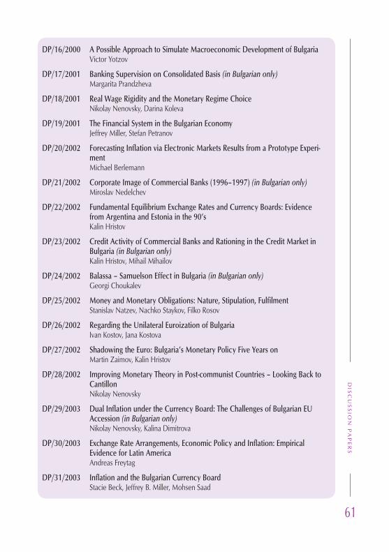
61

DIS

CU

SS

ION

PA

PE

RS

DP/16/2000 A Possible Approach to Simulate Macroeconomic Development of BulgariaVictor Yotzov

DP/17/2001 Banking Supervision on Consolidated Basis (in Bulgarian only)Margarita Prandzheva

DP/18/2001 Real Wage Rigidity and the Monetary Regime ChoiceNikolay Nenovsky, Darina Koleva

DP/19/2001 The Financial System in the Bulgarian EconomyJeffrey Miller, Stefan Petranov

DP/20/2002 Forecasting Inflation via Electronic Markets Results from a Prototype Experi-mentMichael Berlemann

DP/21/2002 Corporate Image of Commercial Banks (1996–1997) (in Bulgarian only)Miroslav Nedelchev

DP/22/2002 Fundamental Equilibrium Exchange Rates and Currency Boards: Evidence from Argentina and Estonia in the 90’sKalin Hristov

DP/23/2002 Credit Activity of Commercial Banks and Rationing in the Credit Market in Bulgaria (in Bulgarian only)Kalin Hristov, Mihail Mihailov

DP/24/2002 Balassa – Samuelson Effect in Bulgaria (in Bulgarian only)Georgi Choukalev

DP/25/2002 Money and Monetary Obligations: Nature, Stipulation, FulfilmentStanislav Natzev, Nachko Staykov, Filko Rosov

DP/26/2002 Regarding the Unilateral Euroization of BulgariaIvan Kostov, Jana Kostova

DP/27/2002 Shadowing the Euro: Bulgaria’s Monetary Policy Five Years on Martin Zaimov, Kalin Hristov

DP/28/2002 Improving Monetary Theory in Post-communist Countries – Looking Back to CantillonNikolay Nenovsky

DP/29/2003 Dual Inflation under the Currency Board: The Challenges of Bulgarian EU Accession (in Bulgarian only)Nikolay Nenovsky, Kalina Dimitrova

DP/30/2003 Exchange Rate Arrangements, Economic Policy and Inflation: Empirical Evidence for Latin AmericaAndreas Freytag

DP/31/2003 Inflation and the Bulgarian Currency BoardStacie Beck, Jeffrey B. Miller, Mohsen Saad

62

DP

/90/

2013

DP/32/2003 Banks – Firms Nexus under the Currency Board: Empirical Evidence from BulgariaNikolay Nenovsky, Evgeni Peev, Todor Yalamov

DP/33/2003 Modelling Inflation in Bulgaria: Markup Model (in Bulgarian only)Kalin Hristov, Mihail Mihailov

DP/34/2003 Competitiveness of the Bulgarian EconomyKonstantin Pashev

DP/35/2003 Exploring the Currency Board Mechanics: a Basic Formal ModelJean-Baptiste Desquilbet, Nikolay Nenovsky

DP/36/2003 A Composite Tendency Indicator for Bulgaria’s Industry (in Bulgarian only)Tsvetan Tsalinsky

DP/37/2003 The Demand for Euro Cash: A Theoretical Model and Monetary Policy ImplicationsFranz Seitz

DP/38/2004 Credibility Level of the Bulgarian Exchange Rate Regime, 1991–2003: First Attempt at Calibration (in Bulgarian only)Georgi Ganev

DP/39/2004 Credibility and Adjustment: Gold Standards Versus Currency BoardsJean-Baptiste Desquilbet, Nikolay Nenovsky

DP/40/2004 The Currency Board: ‘The only game in town’ (in Bulgarian only)Kalin Hristov

DP/41/2004 The Relationship between Real Convergence and the Real Exchange Rate: the Case of BulgariaMariella Nenova

DP/42/2004 Effective Taxation of Labor, Capital and Consumption in Bulgaria (in Bulgarian only)Plamen Kaloyanchev

DP/43/2004 The 1911 Balance of Payments of the Kingdom of Bulgaria(in Bulgarian only)Martin Ivanov

DP/44/2004 Beliefs about Exchange Rate Stability: Survey Evidence from the Currency Board in BulgariaNeven T. Valev, John A. Carlson

DP/45/2005 Opportunities of Designing and Using the Money Circulation Balance (in Bulgarian only)Metodi Hristov

DP/46/2005 The Microeconomic Impact of Financial Crises: The Case of Bulgaria Jonathon Adams-Kane, Jamus Jerome Lim

63

DIS

CU

SS

ION

PA

PE

RS

DP/47/2005 Interest Rate Spreads of Commercial Banks in Bulgaria (in Bulgarian only)Mihail Mihailov

DP/48/2005 Total Factor Productivity Measurement: Accounting of Economic Growth in Bulgaria (in Bulgarian only)Kaloyan Ganev

DP/49/2005 An Attempt at Measurement of Core Inflation in Bulgaria (in Bulgarian only)Kalina Dimitrova

DP/50/2005 Economic and Monetary Union on the HorizonDr Tsvetan Manchev, Mincho Karavastev

DP/51/2005 The Brady Story of Bulgaria (in Bulgarian only)Garabed Minassian

DP/52/2005 General Equilibrium View on the Trade Balance Dynamics in BulgariaHristo Valev

DP/53/2006 The Balkan Railways, International Capital and Banking from the End of the 19th Century until the Outbreak of the First World WarPeter Hertner

DP/54/2006 Bulgarian National Income between 1892 and 1924Martin Ivanov

DP/55/2006 The Role of Securities Investor Compensation Schemes for the Development of the Capital Market (in Bulgarian only)Mileti Mladenov, Irina Kazandzhieva

DP/56/2006 The Optimal Monetary Policy under Conditions of Indefiniteness (in Bulgarian only)Nedyalka Dimitrova

DP/57/2007 Two Approaches to Estimating the Potential Output of Bulgaria Tsvetan Tsalinski

DP/58/2007 Informal Sources of Credit and the ‘Soft’ Information Market (Evidence from Sofia)Luc Tardieu

DP/59/2007 Do Common Currencies Reduce Exchange Rate Pass-through? Implications for Bulgaria’s Currency Board Slavi T. Slavov

DP/60/2007 The Bulgarian Economy on Its Way to the EMU: Economic Policy Results from a Small-scale Dynamic Stochastic General Equilibrium FrameworkJochen Blessing

DP/61/2007 Exchange Rate Control in Bulgaria in the Interwar Period: History and Theo-retical ReflectionsNikolay Nenovsky, Kalina Dimitrova

64

DP

/90/

2013

DP/62/2007 Different Methodologies for National Income Accounting in Central and Eastern European Countries, 1950–1990Rossitsa Rangelova

DP/63/2008 A Small Open Economy Model with a Currency Board Feature: the Case of BulgariaIordan Iordanov, Andrey Vassilev

DP/64/2008 Potential Output Estimation Using Penalized Splines: the Case of BulgariaMohamad Khaled

DP/65/2008 Bank Lending and Asset Prices: Evidence from BulgariaMichael Frömmel, Kristina Karagyozova

DP/66/2008 Views from the Trenches: Interviewing Bank Officials in the Midst of a Credit BoomNeven Valev

DP/67/2008 Monetary Policy Transmission: Old Evidence and Some New Facts from BulgariaAlexandru Minea, Christophe Rault

DP/68/2008 The Banking Sector and the Great Depression in Bulgaria, 1924–1938: Interlocking and Financial Sector ProfitabilityKiril Danailov Kossev

DP/69/2008 The Labour Market and Output in the UK – Does Okun’s Law Still Stand?Boris Petkov

DP/70/2008 Empirical Analisys of Inflation Persistence and Price Dynamics in BulgariaZornitsa Vladova, Svilen Pachedjiev

DP/71/2009 Testing the Weak-form Efficiency of the Bulgarian Stock MarketNikolay Angelov

DP/72/2009 Financial Development and Economic Growth In Bulgaria (1991–2006). An Econometric Analysis Based on the Logic of the Production Function)Statty Stattev

DP/73/2009 Autonomy vs. Stability: the Relationship between Internal and External Money in Bulgaria (1879–1912)Luca Fantacci

DP/74/2009 The Size of the Shadow Economy in Bulgaria: A Measurement Using the Monetary Method Hildegart Ahumada, Facundo Alvarado, Alfredo Canavese, NicolЎs Grosman

DP/75/2009 Efficiency of commercial banks in Bulgaria in the wake of EU accessionKiril Tochkov, Nikolay Nenovsky

DP/76/2009 Structural Current Account Imbalances: Fixed Versus Flexible Exchange Rates?Slavi T. Slavov

65

DIS

CU

SS

ION

PA

PE

RS

DP/77/2009 Econometric Forecasting of Bulgaria’s Export and Import FlowsGrigor Stoevsky

DP/78/2009 Explanations for the Real Exchange Rate Development in the New EU Mемber States in TransitionGalina Boeva

DP/79/2009 The Great Depression in the Eyes of Bulgaria’s Inter-war Economists (How History of Economic Thought Could Matter for Today’s Policy Advice)Stefan Kolev

DP/80/2010 Modeling Interest Rates on Corporate Loans in Bulgaria (in Bulgarian only)Mihail Mihailov

DP/81/2010 A Small Open Economy Model with Financial Accelerator for Bulgaria: The Role of Fiscal Policy and the Currency BoardIvan Lozev

DP/82/2010 The Impact of the Global Economic Crisis on Bulgaria’s Accession to the Euro Area (in Bulgarian only)Tsvetelina Marinova

DP/83/2011 Are Long-term Inflation Expectations Well-anchored? Evidence from the Euro Area and the United StatesTsvetomira Tsenova

DP/84/2011 Relative Inflation Dynamics in the EU Accession Countries of Centraland Eastern EuropeHiranya K Nath Kiril Tochkov

DP/85/2011 Trade, Convergence and Exchange Rate Regime: Evidence from Bulgaria and RomaniaEmilia Penkova-Pearson

DP/86/2011 Short-Term Forecasting of Bulgarian GDP Using a Generalized Dynamic Factor ModelPetra Rogleva

DP/87/2011 Wage-setting Behaviour of Bulgarian Firms: Evidence from Survey DataIvan Lozev, Zornitsa Vladova, Desislava Paskaleva

DP/88/2012 The Predictive Power of Some Market Liquidity Risk Measures: An Empirical ApproachAssoc. Prof. Tsvetan Manchev, Ph. D. Daniel Simeonov, Hristo Ivanov, Christian Hausmann

DP/89/2012 Survey Evidence on Price-setting Behaviour of Firms in BulgariaZornitsa Vladova