I N T E R N A T I O N A L M O N E T A R Y F U N D

I M F S T A F F P O S I T I O N N O T E

Antonio Spilimbergo, Steve Symansky, and Martin Schindler

Fiscal Multipliers

SPN/09/11

May 20, 2009

INTERNATIONAL MONETARY FUND

Fiscal Multipliers

Prepared by the Research Department (Antonio Spilimbergo, Steve Symansky, and Martin Schindler)

May 20, 2009

Note: The views expressed herein are those of the authors and should not be attributed to the IMF, its Executive Board, or its management.

2

This note provides background information for policymakers on fiscal multipliers, including quantitative estimates (see table at the end). What is the fiscal multiplier? The fiscal multiplier is the ratio of a change in output (∆Y) to an exogenous change in the fiscal deficit (∆G is used here as a shortcut, it could be also -∆T) with respect to their respective baselines (often potential output and structural deficit, respectively, even though authors use variations of these concepts).1 Depending on the time frame considered (usually a quarter or a year), different multipliers are used:

• The impact multiplier ( )( )

Y tG t

⎛ ⎞Δ≡⎜ ⎟Δ⎝ ⎠

.

• The multiplier at some horizon N ( )( )

Y t NG t

⎛ ⎞Δ +≡⎜ ⎟Δ⎝ ⎠

.

• The peak multiplier, defined as the largest ( )max( )N

Y t NG t

⎛ ⎞Δ +≡⎜ ⎟Δ⎝ ⎠

over any horizon N.

• The cumulative multiplier, defined as the cumulative change in output over the

cumulative change in fiscal expenditure at some horizon N 0

0

( )

( )

N

jN

j

Y t j

G t j=

=

⎛ ⎞Δ +⎜ ⎟≡⎜ ⎟Δ +⎝ ⎠

∑∑

.

The cumulative multiplier, which is often the most appropriate measure, is typically larger than the impact or peak multipliers, but is rarely reported. Unless specified differently, this note refers to the impact or the peak multiplier, but its implications are broader.2 What determines the size of the multipliers? The size of the multiplier is larger if: a) “leakages” are few (i.e., only a small part of the stimulus is saved or spent on imports), b) the monetary conditions are accommodative (i.e., the interest rate does not increase as a consequence of the fiscal expansion), and c) the country’s fiscal position after the stimulus is sustainable. a) “Leakages” are minimized if: • The stimulus package has a higher government spending component, relative to tax

cuts, as the first round effect on demand is immediate, while individuals may save (part of) a tax cut.

• The marginal propensity to consume is large. • The measures are targeted toward liquidity constrained consumers. • The consumers do not take fully into account large increases in future taxes to

compensate for the debt increase, either because of finite life considerations, or simple myopia (i.e., they do not increase current saving).

1 Unless otherwise indicated, the discussion in this note refers to a temporary change in fiscal policy. 2 Many empirical studies listed in the table below report multipliers at selected horizons without necessarily taking a stance on the value of the peak multiplier.

3

• The propensity to import is small (so large countries and/or countries only partially open to trade have larger multipliers).3

• The automatic stabilizers are small, thereby limiting the revenue and spending offsets to the output response.4

• The size of the output gap is large, and thus the monetary authority can accommodate the increase in demand without having to increase interest rates. Fiscal expansion undertaken when the economy is at, or near, full employment will have limited overall real effects.

b) Monetary conditions are accommodative if: • The nominal interest rate does not increase in response to fiscal expansion, so that

there is less displacement (crowding out) of domestic investment and/or consumption. • The exchange rate is fixed. Accommodative monetary conditions can increase the size of multipliers by a factor of 2 to 3. On the contrary, under plausible assumptions the multiplier is zero if monetary policy is firmly targeting inflation or nominal income. c) Fiscal sustainability reduces the effects that the higher debt has on the long-term interest rates. Can the fiscal multiplier be negative? Yes, fiscal expansions can be contractionary if they decrease consumers’ and investors’ confidence, especially if the fiscal expansion raises, or reinforces, fiscal sustainability concerns.5 What is the size of the fiscal multiplier? The size of the fiscal multiplier is country-, time-, and circumstance-specific. In the March 2009 IMF staff note prepared for the G-20 Ministerial Meeting, a range of multipliers was used.6 The low set of multipliers included 0.3 on revenue, 0.5 on capital spending, and 0.3 on other spending. The high set of multipliers included 0.6 on revenue, 1.8 on capital spending, and 1 for other spending. Cross-country VAR estimates of fiscal multipliers in LICs range from negative to 0.5, in part because of higher fiscal sustainability concerns in LICs. However, these estimates can be downward biased because the lack of accurate data leads to attenuation bias. The table below provides a detailed survey of the estimated multipliers. Which multipliers should be used in specific applications and projections? Fiscal multipliers have been calculated for some countries but should be carefully re-examined in light of the current events. The table below summarizes estimates of multipliers, mostly for advanced countries. Country circumstances, however, should be

3 Investment in public infrastructure that is labor intensive is likely to have a lower import content. 4 However, during downturns, the stabilizers will result in automatic fiscal stimulus, which can compensate for the lower multipliers. 5 There is a large literature on the symmetric case, namely expansionary fiscal contractions. 6 Available at http://www.imf.org/external/np/g20/pdf/031909a.pdf

4

taken into account in arriving at the multiplier for a specific country. The factors mentioned at the beginning should be considered. A rule of thumb is a multiplier (using the definition ∆Y/∆G and assuming a constant interest rate) of 1.5 to 1 for spending multipliers in large countries, 1 to 0.5 for medium sized countries, and 0.5 or less for small open countries. Smaller multipliers (about half of the above values) are likely for revenue and transfers while slightly larger multipliers might be expected from investment spending. Negative multipliers are possible, especially if the fiscal stimulus weakens (or is perceived to weaken) fiscal sustainability. Does the size of the multipliers depend on the degree of financial market development? The degree of financial market development has an ambiguous effect on multipliers, depending on a) how the degree of financial development affects liquidity constraints and b) the government’s ability to finance the fiscal deficit. a) Poorly developed financial markets limit the ability for consumption (and investment) smoothing, which should increase multipliers. b) The effect of government deficits on interest rates depends on the degree of financial development: • In countries with limited access to financial markets, governments can issue debt to

finance a deficit only at very high interest rates, which decreases the size of multipliers.7

• However, in financially repressed countries, governments can issue bonds to ‘captive’ domestic savers, thereby lowering the costs of financing, which raises the size of multipliers.

How does the financial crisis impact the size of multipliers? The impact of the crisis on the size of multipliers is uncertain because: • The uncertainty has probably induced consumers to increase precautionary saving

(e.g., based on aggregate data, the 2008 U.S. tax rebate appears to have been largely saved), reducing the marginal propensity to consume and the size of multipliers.

• The ongoing deleveraging has likely increased the proportion of credit constrained consumers and firms, raising the size of multipliers.

• Monetary policy is extremely accommodative, with the short rate close to zero, and a commitment to keep it there for as long as needed, increasing considerably the size of multipliers.

Do institutional features influence the size of fiscal multipliers? Yes, but taking these features into account generally requires additional information about the specific policy measures. For example, policies vary in efficiency (e.g., developing a new social safety net is more difficult than enhancing existing ones) and 7 In particular, in emerging markets that have just begun developing their financial markets, investors are quite sensitive to assessments of government sustainability, resulting in possibly strong increases in interest rates in government bonds.

5

time of implementation (e.g., new investment projects take longer than speeding up the delivery of existing investment projects). Do temporary or permanent changes in fiscal policy produce larger multipliers? It depends on the fiscal measure. Temporary reductions in income taxes reduce concerns about sustainability (and adverse impact on risk premia) but, to the extent that consumers are forward looking, have less effect on consumption. However, temporary measures that trigger intertemporal reallocation, such as temporary decreases in taxes on automobiles, or in VAT rates, or investment tax credits for firms, can be powerful (although small VAT cuts may not be “visible enough” to prompt a reaction; moreover, the effect of any cut in indirect taxes would depend on the extent to which it is passed through). As a rule of thumb, permanent measures give a higher multiplier than temporary measures in interventions that work through income (e.g., tax cuts), while the reverse is true for interventions that work through prices (e.g., VAT reductions, investment tax credits) because changes in relative intertemporal prices are more likely to affect intertemporal consumption patterns.8 Are multipliers reliable? How are they calculated? The profession disagrees on the reliability of the multipliers, partly because of methodological differences, and partly because the range of estimates, even for similar methodologies, is often quite large. The main empirical challenge is simultaneity bias. For example, a successful fiscal expansion in response to a negative exogenous shock would result in an increase in the deficit with little change in output (leading inappropriately to the conclusion that multipliers are low). The use of higher frequency data, in the presence of implementation lags in fiscal policy with respect to the output shock, reduces the risk of simultaneity bias. There are four broad methodologies to calculate fiscal multipliers: • Model simulations. Models with an underlying ISLM structure and little or no

forward looking behavior result in positive multipliers by construction. An increase in the deficit leads to an increase in demand, which leads to an increase in output. The multipliers are small or negative only if fiscal sustainability is in question, economic agents are forward looking, or monetary policy is not accommodative.

• Case studies. The crucial point is identifying good ‘experiments’, i.e., episodes of truly exogenous fiscal expansion. A good example is the Romer and Romer (2008) study on tax policy changes. An important drawback of case studies is that the results are specific to the type of fiscal measure studied, the prevailing macroeconomic conditions at the time of implementation, etc.

• Vector auto-regressions (VARs). The crucial point is again to correctly identify exogenous movement in public expenditure or taxes. As case studies, VARs give the response of the economy, taking implicitly into account the monetary policy response, and thus the effects on the interest rates (whether or not interest rates are

8 The Elasticity of Intertemporal Substitution (EIS) (i.e., the percentage by which current consumption increases relative to future consumption in response to a percentage change in the ratio between present and future prices) can be assumed to equal 1 for nondurable goods.

6

included in the VAR). Structural model simulations, by contrast, can deliver multipliers given interest rates.

• Econometric studies of consumer behavior in response to fiscal shocks. When these focus on the response of individual consumption to the change in income, they give only the direct, partial equilibrium, effect of the fiscal measure on spending.

All methodologies have shortcomings and caveats. Any estimate of a multiplier should have in mind the assumptions under which it is valid. Is it a good idea to re-estimate the size of fiscal multipliers in the present situation? Probably not, as the current economic situation is unique and the structural parameters have changed, negating a crucial estimation assumption. Past research on multiplier estimates, such as the studies summarized in the table below, can provide guidance in developing multiplier estimates, but judgment, based on current conditions, is important.

Survey of Fiscal Multipliers in the Literature (G= government spending. T= taxes. Z= government investment. VAR= vector auto regression.)

Source Methodology Country Fiscal Shock

One quarter One year Two

yearsThree years

Cumulative over two years (where

applicable)

France Indirect tax 0.3 0.2 0.5Corporate tax lump sum 0.0 0.2 0.2Corporate tax rate 0.2 0.4 0.5Direct tax 0.3 0.2 0.4Transfers 0.2 0.1 0.3

Germany Indirect tax 0.5 0.2 0.7Corporate tax lump sum 0.1 0.6 0.7Corporate tax rate 0.2 0.7 0.8Direct tax 0.7 0.2 0.9Transfers 0.5 0.1 0.6

Italy Indirect tax 0.2 0.2 0.4Corporate tax lump sum 0.0 0.2 0.3Corporate tax rate 0.2 0.4 0.6Direct tax 0.2 0.2 0.3Transfers 0.1 0.1 0.3

Spain Indirect tax 0.2 0.1 0.3Corporate tax lump sum 0.0 0.1 0.2Corporate tax rate 0.2 0.2 0.5Direct tax 0.2 0.1 0.2Transfers 0.1 0.1 0.2

United States G, DT 0.8 0.5 0.5 1.1 1.1G, ST 0.9 0.6 0.7 0.7 1.3T, DT 0.7 0.7 0.7 0.4 1.4T, ST 0.7 1.1 1.3 1.3 2.3

Broda and Parker (2008) /2 Econometric case study of the 2008 tax rebate.

United States Tax rebate 0.2

Implicit control for interest rates through fixed effects.

Bryant and others (1988) /3 United States G 0.6 to 2 0.5 to 2.1 0.5 to 1.7 1.1 to 4.1

Multipliers at Different Horizons

Quarterly structural VAR. No explicit control for interest rates or money supply. Sample: 1960:Q1–1997:Q4.

Comparison of various frameworks (econometric, VAR, and model- simulations). Varying assumptions about the interest rate response.

NiGEM model with one-year shock. Taylor interest rate rule assumed to meet domestic inflation targets.

Blanchard and Perotti (2002) /1

Al-Eyd and Barrell (2005)

7

Source Methodology Country Fiscal Shock

One quarter One year Two

yearsThree years

Cumulative over two years (where

applicable)

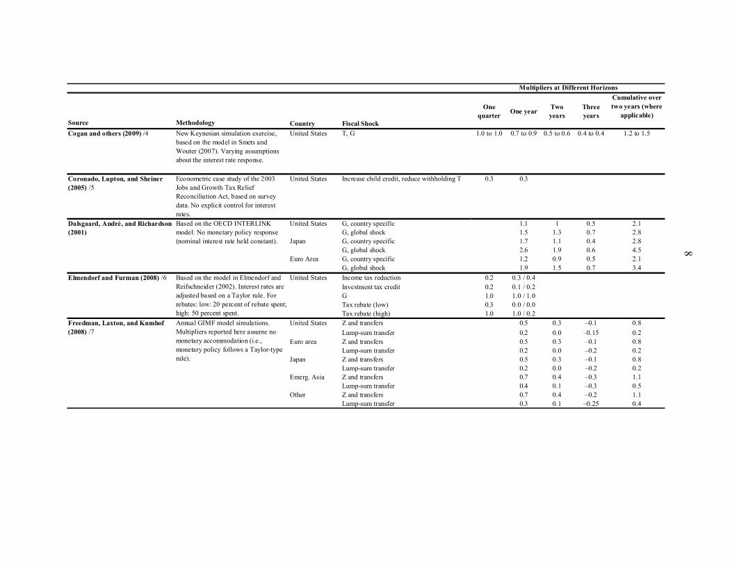
Cogan and others (2009) /4 New Keynesian simulation exercise, based on the model in Smets and Wouter (2007). Varying assumptions about the interest rate response.

United States T, G 1.0 to 1.0 0.7 to 0.9 0.5 to 0.6 0.4 to 0.4 1.2 to 1.5

Coronado, Lupton, and Sheiner (2005) /5

Econometric case study of the 2003 Jobs and Growth Tax Relief Reconciliation Act, based on survey data. No explicit control for interest rates.

United States Increase child credit, reduce withholding T 0.3 0.3

United States G, country specific 1.1 1 0.5 2.1G, global shock 1.5 1.3 0.7 2.8

Japan G, country specific 1.7 1.1 0.4 2.8G, global shock 2.6 1.9 0.6 4.5

Euro Area G, country specific 1.2 0.9 0.5 2.1G, global shock 1.9 1.5 0.7 3.4

United States Income tax reduction 0.2 0.3 / 0.4Investment tax credit 0.2 0.1 / 0.2G 1.0 1.0 / 1.0Tax rebate (low) 0.3 0.0 / 0.0Tax rebate (high) 1.0 1.0 / 0.2

United States Z and transfers 0.5 0.3 –0.1 0.8Lump-sum transfer 0.2 0.0 –0.15 0.2

Euro area Z and transfers 0.5 0.3 –0.1 0.8Lump-sum transfer 0.2 0.0 –0.2 0.2

Japan Z and transfers 0.5 0.3 –0.1 0.8Lump-sum transfer 0.2 0.0 –0.2 0.2

Emerg. Asia Z and transfers 0.7 0.4 –0.3 1.1Lump-sum transfer 0.4 0.1 –0.3 0.5

Other Z and transfers 0.7 0.4 –0.2 1.1Lump-sum transfer 0.3 0.1 –0.25 0.4

Multipliers at Different Horizons

Annual GIMF model simulations. Multipliers reported here assume no monetary accommodation (i.e., monetary policy follows a Taylor-type rule).

Dalsgaard, André, and Richardson (2001)

Elmendorf and Furman (2008) /6

Freedman, Laxton, and Kumhof (2008) /7

Based on the OECD INTERLINK model. No monetary policy response (nominal interest rate held constant).

Based on the model in Elmendorf and Reifschneider (2002). Interest rates are adjusted based on a Taylor rule. For rebates: low: 20 percent of rebate spent; high: 50 percent spent.

8

Source Methodology Country Fiscal Shock

One quarter One year Two

yearsThree years

Cumulative over two years (where

applicable)

Heathcote (2005) /8 Calibrated (real) model with distortionary taxation and capital market imperfections. No modeling of monetary policy.

United States T (temporary proportional income tax reduction)

0.4

Germany T 0.2G 0.4

Spain T 0.1G 0.5

France T 0.1G 0.5

Ireland T 0.1G 0.4

Italy T 0.1G 0.5

Netherlands T 0.1G 0.4

Portugal T 0.0 to 0.1G 0.7

Sweden T 0.3G 0.4

United Kingdom T 0.2G 0.3

High-income G 0.4 0.7 0.9 0.8 1.5Developing G 0.6 0.4 0.1 –0.11 0.5

IMF (2008) /11 Advanced T 0.4 / 0.0 0.6 / 0.4G –0.1 / 0.2 –0.3 / 0.5

Emerging T 0.2 / 0.1 0.2 / 0.2G 0.2 / 0.1 –0.2 / –0.2

Multipliers at Different Horizons

Quarterly panel VAR on 27 developing and 22 high-income countries. No explicit control for (country-specific) interest rates (only U.S. interest rate included).Regression analysis using annual panel data for advanced and emerging economies. Two alternative measures of the fiscal impulse (elasticity/regression based.) Real money growth is included as a control for monetary policy.

European Commission's QUEST model.Interest rates respond to meet EU area inflation targets (except Sweden and the UK, which are assumed to target their own inflation rates).

HM Treasury (2003) /9

Ilzetzki and Végh (2008) /10

9

Source Methodology Country Fiscal Shock

One quarter One year Two

yearsThree years

Cumulative over two years (where

applicable)

Johnson, Souleles, and Parker (2006) /12

Survey data used to study the effect of the 2001 tax rebate. Authors consider household impact responses. Any effect from interest rates would come through household expectations.

United States Tax rebates 0.2 to 0.4 0.7

Australia G –0.1 / 0.4 1.4 / 0.7T –1.5 / –.6 –1.7 / –.9

Canada G 1.0 / –0.3 0.6 / –1.1T –0.4 / 0.4 –0.2 / 1.6

Germany G 0.6 / 0.5 –0.8 / –1.1T –0.3 / 0.0 0.1 / –0.6

United Kingdom G 0.5 / –0.3 0.0 / –0.9T 0.2 / –0.4 0.2 / –0.7

United States G 1.3 / 0.4 1.7 / 0.1T 1.4 / –0.7 23.9 / –1.6

Australia G 0.6 0.9 0.9Z –0.3 0.0 0.5

Canada G 0.6 0.7 0.9Z 0.4 –0.2 –0.7

Germany G 0.8 0.8 0.9Z 5.1 4.4 3.8

United Kingdom G 0.6 0.9 1.0Z 0.0 –0.1 –0.1

United States G 1.4 1.9 2.2Z 1.2 0.5 0.2

Ramey (2008) /15 Quarterly VAR. Narrative approach to identify military buildups. No explicit control for interest rates. Sample: 1947:Q1–2003:Q4.

United States Military spending ≈ 1.5 ≈ 0 < 0 1.5

Multipliers at Different Horizons

Perotti (2005) /13 Quarterly VAR. Ten-year nominal interest rate included in the VAR. Time coverage varies by country as follows: Australia: 1960:Q1–2001:Q2, Canada: 1961:Q1–2001:Q4, Germany: 1960:Q1–1989:Q4, UK: 1963:Q1–2001:Q2, US: 1960:Q1–2001:Q4.Multipliers reported are cumulative.

Perotti (2006) /14 Quarterly VAR. Ten-year nominal interest rate included in the VAR. Time coverage varies by country as follows: Australia: 1960:1 2001:2, Canada: 1961:1-2001:4, Germany: 1960:1-1989:4, UK: 1963:1-2001:2, US: 1960:1-2001:4. Multipliers reported are cumulative.

10

Source Methodology Country Fiscal Shock

One quarter One year Two

yearsThree years

Cumulative over two years (where

applicable)

Romer and Romer (2008) /16 Narrative, single equations and VARs. Explicit control for interest (federal funds) rates in some specifications. Sample: 1945–2007.

United States T 1.2 2.8 2.7 4.0

Zandi (2008) United States Tax rebate 1.0 / 1.3Payroll tax holiday 1.3Tax cut 1.0Accelerated depreciation 0.3Extension of alternative minimum tax patch 0.5Bush income tax cuts permanent 0.3Dividend and capital gains tax cuts permanent 0.4Cut corporate tax rate 0.3

1.61.71.4

Infrastructure spending 1.6

Moody’s Economy.com macro model. (Details of the model are not specified.) The two tax rebate multipliers are from nonrefundable and refundable rebates.

Extension of unemployment insurance benefitsTemporary increase of food stampsGeneral aid to state governments

Multipliers at Different Horizons

Note: Prepared by Lone Christiansen and Martin Schindler. “Fiscal multiplier” here refers to ∆Y(t+N)/∆G(t), where N can be one quarter (impact multiplier), one year, two years, or three years. Unless noted otherwise, the multipliers indicate the output response at different horizons, relative to the baseline, without a fiscal stimulus, as a result of a given temporary fiscal shock at time t, to be interpreted as the dollar increase in output at time t+N for each $1 of fiscal stimulus at time t. The last column shows staff calculations of the two-year cumulative output response, approximated by the (weighted) sum of the fiscal multipliers in the “one quarter,” “one year,” and “two years” columns. Where no data are available at either the one- or the two-year horizon, no cumulative multiplier is calculated. For an additional overview of multipliers, see Hemming and others (2002). /1 DT = deterministic trend; ST = stochastic trend. See Tables 3 and 4 in Blanchard and Perotti (2002). /2 The within-quarter numbers are numbers for nondurable goods spending within the first month after receipt of the tax rebate. This estimate is extrapolated from estimates by Johnson, Souleles, and Parker (2006) on the 2001 U.S. tax rebates. /3 Comparison of several different models. Foreign monetary aggregates are held unchanged from the baseline. Numbers are approximate readings from a graph. The study also reports results from the Minneapolis World VAR Model. This model has a one-year multiplier close to zero. /4 The estimates from Cogan and others (2009) are based on the output effects in the Smets-Wouters (2007) model, assuming a permanent 1 percent increase in G. The range of values arises from different assumptions regarding the interest rate response. /5 The within-quarter estimates are within two quarters of the change. /6 The one-year responses are responses in the second and third quarters after the stimulus.

11

/7 Year one is the first year with output effects. The shock is a global fiscal expansion. The combination shock (Z and transfers) is a combination of government investment and lump-sum transfers. Numbers are approximate, based on readings from an impulse response function. The authors also report multipliers when monetary policy is more accommodative (with policy rates held constant for one or two years following the fiscal impulse)—output responses are larger in those cases. /8 The output multiplier is calculated by IMF staff based on Tables 1 and 8 in Heathcote (2005) according to: –ΔY/ΔT = –%ΔY/%ΔT·Y/T = –.62/(–6.24)·1/.26 = .38. /9 The multipliers from taxes result from a combination of labor, corporate profits, and value-added taxes. /10 G refers to government consumption. Most of the multipliers reported are based on elasticity readings from a graph, translated to multipliers, with the authors’ reported government consumption shares according to ΔY/ΔG = %ΔY/%ΔG·Y/G. /11 The two numbers in each cell are based on elasticity- and regression-based fiscal impulse measures, respectively. The T measure is a revenue-based policy change,and the G measure denotes an expenditure-based policy change. See Table 5.4 in IMF (2008). /12 Study of the effect on nondurable consumption. The one-year multiplier estimate is for the three-month period of rebate receipt and the following three-month period. /13 Perotti (2005) reports cumulative cyclically adjusted multipliers (i.e., the ratio of the cumulative response of GDP at quarter t to the cumulative response of cyclically adjusted government spending at the same quarter) at annual rates. The two multipliers reported are for the early and the late part of his sample, respectively. The high value for the United States should be interpreted with caution, since the standard error bands around the estimate include zero. /14 Perotti (2006) reports cumulative multipliers (i.e., the cumulative response of GDP to a fiscal shock divided by the sum of the cumulative responses of the fiscal variable itself) at annual rates. G denotes government consumption. /15 The estimates reported in Ramey (2008, Figure 5A, second column) are “fiscal elasticities,” corresponding to %ΔY/%ΔG in our notation. Fiscal multipliers are derived by multiplying the “fiscal elasticity” by Y/G, which at the peak of Ramey’s estimated impulse response function (four quarters) corresponds to %ΔY/%ΔG·Y/G ≈ 0.3·5 = 1.5. /16 Numbers are approximate, based on readings from an impulse response function (Romer and Romer, 2008, Figure 5) and for the case without controls for interest rates or other monetary policy indicators. When those are controlled for, the fiscal multipliers are about 20 to 30 percent smaller.

12

13

References Al-Eyd, Ali J., and Ray Barrell, 2005, “Estimating Tax and Benefit Multipliers in

Europe,” Economic Modelling, Vol. 22, pp. 759–76.

Blanchard, Olivier, and Roberto Perotti, 2002, “An Empirical Characterization of the Dynamic Effects of Changes in Government Spending and Taxes on Output,” Quarterly Journal of Economics, Vol. 117, pp. 1329–1368.

Broda, Christian, and Jonathan Parker, 2008, “The Impact of the 2008 Tax Rebate on Consumer Spending: Preliminary Evidence” (unpublished: University of Chicago Graduate School of Business).

Bryant, Ralph, Dale Henderson, Gerald Holtham, Peter Hooper, and Steven Symansky, 1988, Empirical Macroeconomics for Interdependent Economies, Supplemental Volume (Washington: Brookings Institution).

Cogan, John F., Tobias Cwik, John B. Taylor, and Volker Wieland, 2009, “New Keynesian versus Old Keynesian Government Spending Multipliers,” NBER Working Paper No. 14782 (Cambridge: NBER).

Coronado, Julia Lynn, Joseph P. Lupton, and Louise M. Sheiner, 2005, “The Household Spending Response to the 2003 Tax Cut: Evidence from Survey Data,” Federal Reserve Board Discussion Paper No. 2005-32 (Washington).

Dalsgaard, Thomas, Christophe André, and Pete Richardson, 2001, “Standard Shocks in the OECD Interlink Model,” OECD Economics Department Working Paper No. 306 (Paris: Organization for Economic Cooperation and Development).

Elmendorf, Douglas W., and Jason Furman, 2008, “If, When, How: A Primer on Fiscal Stimulus,” Hamilton Project Strategy Paper (Washington: Brookings Institution).

Freedman, Charles, Douglas Laxton, and Michael Kumhof, 2008, “Deflation and Countercyclical Fiscal Policy” (unpublished; Washington, International Monetary Fund).

Heathcote, Jonathan, 2005, “Fiscal Policy with Heterogeneous Agents and Incomplete Markets,” Review of Economic Studies, Vol. 72, pp. 161–88.

Hemming, Richard, Michael Kell, and Selma Mahfouz, 2002, “The Effectiveness of Fiscal Policy in Stimulating Economic Activity—A Review of the Literature,” IMF Working Paper No. 02/208 (Washington, International Monetary Fund).

HM Treasury, 2003, “Fiscal Stabilisation and EMU,” discussion paper (London).

14

Ilzetzki, Ethan, and Carlos A. Végh, 2008, “Procyclical Fiscal Policy in Developing Countries: Truth or Fiction?” NBER Working Paper No. 14191 (Cambridge, Massachusetts: National Bureau of Economic Research).

International Monetary Fund (IMF), 2008, “Fiscal Policy as a Countercyclical Tool,” Chapter 5 in World Economic Outlook (Washington, October), pp. 159–96.

Johnson, D., Nicolas Souleles, and Jonathan Parker, 2006, “Household Expenditure and the Income Tax Rebates of 2001,” American Economic Review, Vol. 96, pp. 1589–1610.

Perotti, Roberto, 2005, “Estimating the Effects of Fiscal Policy in OECD Countries,” CEPR Discussion Paper No. 4842 (London: Centre for Economic Policy Research).

———, 2006, “Public Investment and the Golden Rule: Another (Different) Look,” IGIER Working Paper No. 277 (Milan: Bocconi University Innocenzo Gasparini Institute for Economic Research).

Ramey, Valerie, 2008, “Identifying Government Spending Shocks: It’s All in the Timing” (unpublished; University of California, San Diego).

Romer, Christina, and David Romer, 2008, “The Macroeconomic Effects of Tax Changes: Estimates Based on a New Measure of Fiscal Shocks” (unpublished; University of California, Berkeley).

Smets, Frank, and Raf Wouters, 2007, “Shocks and Frictions in U.S. Business Cycles: A Bayesian DSGE Approach,” American Economic Review, Vol. 97, pp. 506–606.

Zandi, Mark, 2008, “A Second Quick Boost From Government Could Spark Recovery,” edited excerpts from July 24, 2008, testimony by Mark Zandi, chief economist of Moody’s Economy.com, before the U.S. House of Representatives Committee on Small Business.