Fiscal Federalism and Legislative Malapportionment:

Causal Evidence from Independent but Related Natural Experiments1

Sebastian Galiani2

University of Maryland

Iván Torre3

Sciences Po

Gustavo Torrens4

Indiana University

January, 2015

Abstract: We exploit three natural experiments in Argentina in order to study the role of legislative

malapportionment on the biased federal tax sharing scheme prevalent in the country. We do not find

support to attribute it to legislative malapportionment during periods when democratic governments were

in place; nor did we find any evidence that the tax sharing distribution pattern became less biased under

centralized military governments. We argue that these results are attributable to two of Argentina’s

institutional characteristics: first, the predominance of the executive branch over the legislature; and,

second, the lack of any significant difference in the pattern of geographic representation in the executive

branch under democratic and autocratic governments. Thus, the observed biases in the distribution of tax

revenues among the Argentine provinces are not caused by legislative malapportionment, but are instead

the result of a more structural political equilibrium.

Keywords: Malapportionment; Fiscal Federalism and Natural Experiments.

JEL-Codes: D72; D78 and H3.

1 We would specially like to thank Daron Acemoglu, Michael Alexeev, Marcela Eslava, John Wallis and seminar participants in various places for insightful comments. 2 Email address: galiani@econ.umd.edu 3 Email address: ivan.torre@sciencespo.fr 4 Email address: gtorrens@indiana.edu

1

1. Introduction

Many legislatures are not well apportioned, with some constituencies having a larger or smaller share of

seats than would be dictated by the relative sizes of their populations. According to the mainstream

literature on legislative bargaining, malapportionment should lead to the formulation of biased policies

that mirror the overrepresentation or underrepresentation of different constituencies. However, these

same biases could also be generated by other economic and institutional factors. This paper explores the

question as to whether certain policy biases are actually caused by legislative malapportionment or are the

outcome of a more structural type of political equilibrium. In particular, we exploit three natural

experiments that occurred in Argentina in order to estimate the extent of the effects of legislative

malapportionment on the Argentine federal tax sharing scheme.

Baron and Ferenjohn (1989), in their seminal model of legislative bargaining, show that political outcomes

in a legislature are determined by the distribution of bargaining power among different legislators.

Consequently, any shift in the balance of bargaining power in favor of (or against) a particular legislator

will result in a change in the equilibrium point toward (or against) her constituency’s bliss point. If we

apply this model to a federal State or, indeed, to any polity made up of several political entities (states,

provinces, local governments), the inevitable conclusion is that overrepresented political entities can be

expected to receive favorable treatment5. This is the malapportionment hypothesis.

A few papers exploit plausible exogenous variation in legislative representation to test the

malapportionment hypothesis. Horiuchi and Saito (2003) find empirical support for the hypothesis that

malapportionment leads to policy outcomes that favor overrepresented districts. Using municipal-level

data from Japan, they show that municipalities in overrepresented districts received higher subsidies per

capita than those located in underrepresented ones. They exploit the fact than in 1994 an electoral reform

bill significantly altered the geographical allocation of seats in the national legislature, which provided a

source of exogenous variation in the degree of representation of each district. Ansolabehere, Gerber and

Snyder (2002) provide similar evidence for legislative districts in the United States using court-ordered

redistricting in the 1960s as a source of an exogenous variation in the distribution of geographic

5 In bicameral legislatures where one chamber is malapportioned and the other is not this result will depend on which chamber initiates the legislative process (Ansolabehere, Snyder and Ting, (2003) ).

2

representation6. Dragu and Rodden (2011) focus on resource allocation at the state level in countries with

federal governments and find that overrepresentation has a positive effect on the size of fund transfers. In

order to overcome potential endogeneity problems, they exploit the fact that new states were added to

many federations over time. The idea is that, unlike the states that were originally a part of a federal system,

these new states did not participate in the formulation of the representation rule that was put in place and,

therefore, their funding allocations can be expected to correspond more to the rule itself rather than to

what the authors refer to as the “original bargaining” terms arranged upon by founding states7.

Our study introduces three distinguishing features in order to control for potential endogeneity problems.

First, we exploit the fact that, in Argentina, on three occasions (1960, 1973 and 1983) changes were made

in the minimum number of legislators per district. These changes increased the number of seats in the

smaller districts and modified the total number of seats, thereby altering the legislative representation of

each district. Second, as in Dragu and Rodden (2011), we exploit the fact in 1953, 1955, 1958 and 1991

new provinces were added to the Argentine federation by focusing on the effect that these additions had

on the legislative representation of the original 15 provinces8. Using this strategy, we obtain exogenous

variations for the legislative representation of those 15 provinces. Third, we exploit the country’s

exceptional degree of institutional volatility, which induces a radical exogenous variation in the level of

legislative representation. Specifically, during the time covered by our dataset, there were numerous

military coups (five in total: 1943, 1955, 1962, 1966 and 1976 – the first coup in Argentina in 1930 is out

of our sample) that gave rise to several autocracies. In each of these periods, Congress was shut down and

the president, who was appointed by the military, centralized legislative power. Thus, under military

governments, legislative malapportionment was eliminated completely. Moreover, the civil governors of

6 Gordin (2010) and Turgeon and Cavalcante (2012) present evidence of a positive association between malapportionment and transfers from the central government in Argentina and Brazil respectively. Gibson, Calvo and Faletti (2004) present similar findings for a bigger group of countries with federal systems of government. 7 On a different perspective, Bruhn, Gallego and Onorato (2010) argue that legislative malapportionment may be the result of a strategy devised by pre-democratic elites to retain political influence in democracy, and using data from Latin America they show that overrepresented districts usually vote for the elites’ parties. 8 Actually they were 14 provinces and the City of Buenos Aires, which is not a province but has a large degree of autonomy. Throughout this paper we will refer to them, for the sake of simplicity, as 15 provinces.

3

the provinces were mostly replaced by members of the armed forces, which acted as delegates of the

central government9.

We have built up a database that covers the changes that have occurred in the Argentine tax sharing scheme

since its inception in 1935 up to 2011. We have also collected data on the legislative representation of the

Argentine provinces from 1935 to 2011. Thus, we have a panel dataset that encompasses both trends in

the transfers received by each province through the tax sharing scheme and trends in the representation

of each province. We use our dataset to estimate the effect of changes in legislative representation on the

transfers received by the provinces. We find that there is no statistical evidence to support the idea that

legislative malapportionment has a causal effect on the federal tax sharing scheme in the country studied.

We also find that there is no evidence to support the thesis that, under centralized military governments,

the distribution of revenues under the tax sharing scheme reverted to a more proportional pattern in the

absence of malapportionment.

We then also explore potential explanations for our results. First, we develop a very simple politico-

economic model based on two socioeconomic groups (the rich and the poor), three political jurisdictions

(the federal government and two local government), and one national and two local public goods whose

production is financed by a proportional income tax. We consider two political regimes (democracy and

autocracy) and, following Acemoglu and Robinson (2006), we assume that, under democracy (autocracy),

the poor (rich) are better represented. We show that although democracies and autocracies differ in terms

of the level of taxation and provision of public goods (bigger governments under democracy), they may not

differ to any significant degree in terms of the distribution of resources among districts. In particular, we

show that the share of public revenues received by each local government is the same under a democracy

dominated by the executive branch and under an autocracy, while overrepresented districts receive more

resources under a democracy in which a malapportioned Congress wields power than under an autocracy.

Second, we argue that the executive branch has much more power than the legislative branch in Argentina

and, hence, malapportionment does not have as great an impact as we would otherwise expect when

9 There is little literature on the nature of the institutional relationship between the executive power and the provinces during military regimes in Argentina, but the evidence indicates that many of the delegates had little relationship with the provinces which they were sent to govern.

4

democratic governments are in place. However, the predominance of the executive branch cannot by itself

account for the persistence of these biases or explain why military governments did not revert to a more

proportional pattern of distribution, unless the bargaining process that determines the distribution of tax

revenues among the provinces does not differ very much from one political regime to the next. In order to

further explore this vein, we build an index of geographic representation in the executive branch under

democracy and under military governments. We find that there is no significant difference between

democratic and autocratic government in the ratings, but there is a significant difference between the

degree of geographic representativeness of the executive and legislative branches. This leads us to

conjecture that the biases evident in the Argentine tax sharing system are not a function of legislative

malapportionment, but are instead the outcome of a deeper equilibrium which is robust to the geographic

distribution of legislative representation and the political regime. Nevertheless, further research will be

needed to shed light on this issue.

The rest of this paper is organized as follows. In Section 2, we summarize historical trends in the Argentine

federal tax sharing scheme. In Section 3, we describe the malapportionment of the Argentine Congress. In

Section 4, we explain the estimation strategy, and in Section 5, we present and interpret the main results.

In Section 6, we develop a very simple politico-economic model of fiscal policy in a federation. In Section

7, we explore the question as to why legislative malapportionment does not have an effect on the federal

tax sharing scheme and why the presence of military governments does not significantly change the

scheme. Finally, Section 8 concludes.

2. The Argentine Federal Tax Sharing Scheme

In this section we first briefly summarize the institutional development of fiscal federalism in Argentina,

focusing on the federal tax sharing scheme that was launched in 1935. We then describe the ways in which

the scheme has changed over time.

Following Porto (1990), we can divide the history of fiscal federalism in Argentina into three distinct

periods: (i) the division of tax sources; (ii) competitive federalism; and (iii) the federal tax sharing scheme.

The first period goes from 1853 –when the modern Argentine Constitution was promulgated- to 1890.

During this period, there was a constitutional mandate for a division of tax revenue sources between the

national government and the provinces. The national government collected taxes only on foreign trade,

5

while the provinces collected domestic taxes on consumption and production. Between 1890 and 1934,

there was a period of “competitive federalism” in which both the national government and the provinces

collected taxes on consumption and production. Until that time, intergovernmental transfers had been very

limited in scale and were confined to discretionary transfers from the national government to the

provinces. The last period, from 1935 until the present day, started with the creation of the federal tax

sharing scheme (coparticipación federal de impuestos). Under this scheme, specified types of taxes have

been centralized and are thus collected by the national government, which then redistributes the revenues

among the provinces. See the Online Appendix A for a narrative of the evolution of federal tax sharing

scheme.

2.1. Historical Trends in the Argentine Federal Tax Sharing Scheme

We have built a database that covers trends in the tax sharing scheme since its inception in 1935 up until

2011, which is the last year for which annual data are available. This includes all 24 subnational districts

of the country. In particular, our database registers the amount of money each district has received every

year under the tax sharing scheme and the associated laws. Discretionary transfers have not been taken

into account. All the information comes from official sources, which are all detailed in Appendix B.

A convenient and systematic way of summarizing the aggregate biases in the tax sharing scheme is to

compute the Gini coefficient associated with the distribution of the transfers per capita. Let 𝑡𝑡𝑡𝑡𝑡𝑡𝑡𝑡𝑡𝑡𝑡𝑡𝑡𝑡𝑡𝑡𝑡𝑡𝑖𝑖,𝑡𝑡𝑝𝑝𝑝𝑝𝑝𝑝𝑝𝑝𝑝𝑝𝑡𝑡𝑡𝑡𝑝𝑝𝑝𝑝𝑡𝑡𝑖𝑖,𝑡𝑡

be

the transfers per capita received by province 𝑖𝑖 in year 𝑡𝑡 and suppose that we order provinces according to

this ratio, where 𝑖𝑖 = 1 indicates the province with the lowest transfers per capita and 𝑖𝑖 = 𝑁𝑁 the one with

the highest. Let 𝑝𝑝𝑝𝑝𝑝𝑝𝑝𝑝𝑝𝑝𝑡𝑡𝑡𝑡𝑝𝑝𝑝𝑝𝑡𝑡𝑖𝑖,𝑡𝑡𝑝𝑝𝑝𝑝𝑝𝑝𝑝𝑝𝑝𝑝𝑡𝑡𝑡𝑡𝑝𝑝𝑝𝑝𝑡𝑡𝑡𝑡

be the proportion of the total population that lives in province 𝑖𝑖. Then, the Gini

coefficient of the transfers per capita can be computed as follows:

𝐺𝐺𝑡𝑡𝑇𝑇𝑡𝑡𝑡𝑡𝑡𝑡𝑡𝑡𝑡𝑡𝑡𝑡𝑡𝑡𝑡𝑡 = 1 −

∑ �𝑝𝑝𝑝𝑝𝑝𝑝𝑝𝑝𝑝𝑝𝑝𝑝𝑡𝑡𝑖𝑖𝑝𝑝𝑝𝑝𝑖𝑖,𝑡𝑡𝑝𝑝𝑝𝑝𝑝𝑝𝑝𝑝𝑝𝑝𝑝𝑝𝑡𝑡𝑖𝑖𝑝𝑝𝑝𝑝𝑡𝑡

��𝑆𝑆𝑖𝑖−1,𝑡𝑡+𝑆𝑆𝑖𝑖,𝑡𝑡�𝑁𝑁𝑖𝑖=1

𝑆𝑆𝑁𝑁,𝑡𝑡

where 𝑆𝑆𝑝𝑝,𝑡𝑡 = ∑ �𝑝𝑝𝑝𝑝𝑝𝑝𝑝𝑝𝑝𝑝𝑡𝑡𝑡𝑡𝑝𝑝𝑝𝑝𝑡𝑡𝑗𝑗,𝑡𝑡

𝑝𝑝𝑝𝑝𝑝𝑝𝑝𝑝𝑝𝑝𝑡𝑡𝑡𝑡𝑝𝑝𝑝𝑝𝑡𝑡𝑡𝑡� � 𝑡𝑡𝑡𝑡𝑡𝑡𝑡𝑡𝑡𝑡𝑡𝑡𝑡𝑡𝑡𝑡𝑡𝑡𝑗𝑗,𝑡𝑡

𝑝𝑝𝑝𝑝𝑝𝑝𝑝𝑝𝑝𝑝𝑡𝑡𝑡𝑡𝑝𝑝𝑝𝑝𝑡𝑡𝑗𝑗,𝑡𝑡�𝑝𝑝

𝑗𝑗=1 , and 𝑆𝑆0,𝑡𝑡 = 0.

(1.)

6

𝐺𝐺𝑡𝑡𝑇𝑇𝑡𝑡𝑡𝑡𝑡𝑡𝑡𝑡𝑡𝑡𝑡𝑡𝑡𝑡𝑡𝑡 is a measure of the degree of inequality of the distribution of tax revenues among the provinces

under the federal tax sharing system. Note that if each province receives the same transfer per capita, then

𝐺𝐺𝑡𝑡𝑇𝑇𝑡𝑡𝑡𝑡𝑡𝑡𝑡𝑡𝑡𝑡𝑡𝑡𝑡𝑡𝑡𝑡 = 0, while, at the other extreme, if only one province concentrates all the transfers, then

𝐺𝐺𝑡𝑡𝑇𝑇𝑡𝑡𝑡𝑡𝑡𝑡𝑡𝑡𝑡𝑡𝑡𝑡𝑡𝑡𝑡𝑡 = 1. Figure 1.a shows the trends in 𝐺𝐺𝑡𝑡

𝑇𝑇𝑡𝑡𝑡𝑡𝑡𝑡𝑡𝑡𝑡𝑡𝑡𝑡𝑡𝑡𝑡𝑡 for all the provinces, while Figure 1.b shows

𝐺𝐺𝑡𝑡𝑇𝑇𝑡𝑡𝑡𝑡𝑡𝑡𝑡𝑡𝑡𝑡𝑡𝑡𝑡𝑡𝑡𝑡 for the original 15 provinces.

Figure 1: Gini Coefficient for Per Capita Transfers

As Figure 1 shows, inequality in per capita transfers decreased during the early years of the federal tax

sharing scheme, falling to its lowest point in the early 1950s, and then started to rise again. The same

pattern is observed if we restrict the analysis to the original 15 provinces in the scheme.

The trend in 𝐺𝐺𝑡𝑡𝑇𝑇𝑡𝑡𝑡𝑡𝑡𝑡𝑡𝑡𝑡𝑡𝑡𝑡𝑡𝑡𝑡𝑡 points to major changes in the transfers per capita received by each province

relative to the average transfer per capita (some provinces won and others lost as the tax sharing system

became more or less unequal). In fact, there has been a great deal of variability in the figures for different

provinces. For instance, take the case of Catamarca: from a share of 0.5% of total transfers in 1935, its share

rose to 1.9% in 1973 and 2.7% in 2011. An opposite trend was seen in the case of Mendoza, which had had

7

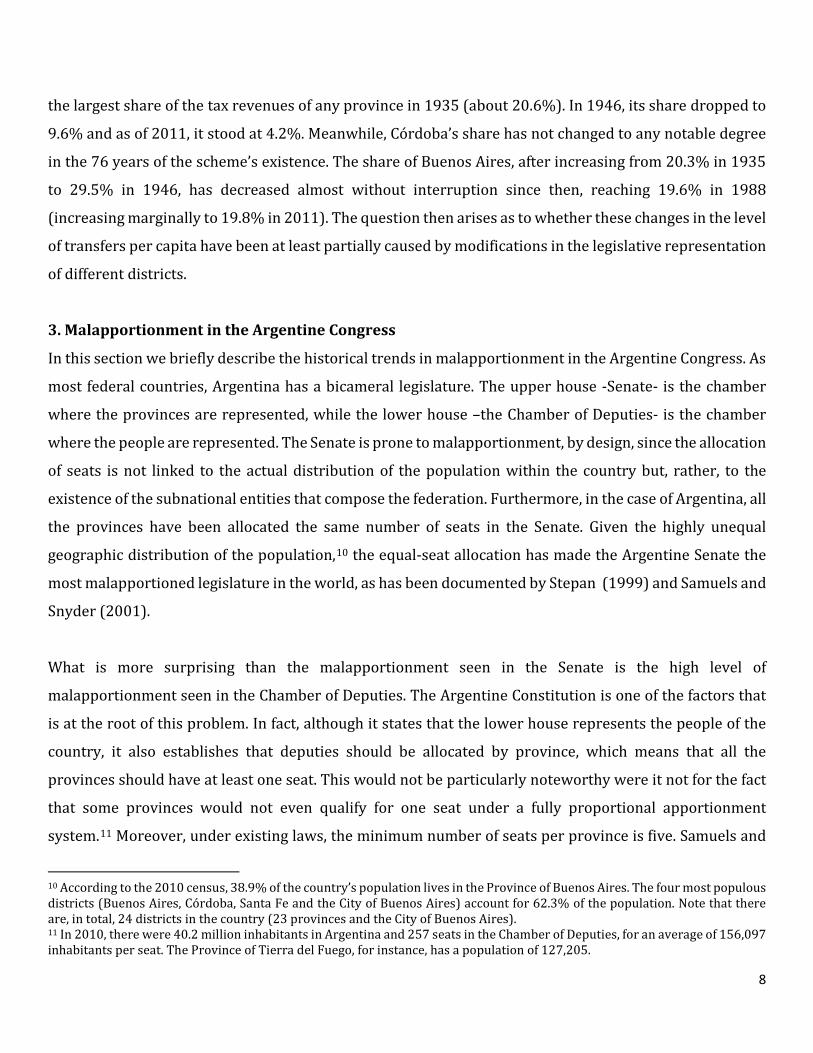
the largest share of the tax revenues of any province in 1935 (about 20.6%). In 1946, its share dropped to

9.6% and as of 2011, it stood at 4.2%. Meanwhile, Córdoba’s share has not changed to any notable degree

in the 76 years of the scheme’s existence. The share of Buenos Aires, after increasing from 20.3% in 1935

to 29.5% in 1946, has decreased almost without interruption since then, reaching 19.6% in 1988

(increasing marginally to 19.8% in 2011). The question then arises as to whether these changes in the level

of transfers per capita have been at least partially caused by modifications in the legislative representation

of different districts.

3. Malapportionment in the Argentine Congress

In this section we briefly describe the historical trends in malapportionment in the Argentine Congress. As

most federal countries, Argentina has a bicameral legislature. The upper house -Senate- is the chamber

where the provinces are represented, while the lower house –the Chamber of Deputies- is the chamber

where the people are represented. The Senate is prone to malapportionment, by design, since the allocation

of seats is not linked to the actual distribution of the population within the country but, rather, to the

existence of the subnational entities that compose the federation. Furthermore, in the case of Argentina, all

the provinces have been allocated the same number of seats in the Senate. Given the highly unequal

geographic distribution of the population,10 the equal-seat allocation has made the Argentine Senate the

most malapportioned legislature in the world, as has been documented by Stepan (1999) and Samuels and

Snyder (2001).

What is more surprising than the malapportionment seen in the Senate is the high level of

malapportionment seen in the Chamber of Deputies. The Argentine Constitution is one of the factors that

is at the root of this problem. In fact, although it states that the lower house represents the people of the

country, it also establishes that deputies should be allocated by province, which means that all the

provinces should have at least one seat. This would not be particularly noteworthy were it not for the fact

that some provinces would not even qualify for one seat under a fully proportional apportionment

system.11 Moreover, under existing laws, the minimum number of seats per province is five. Samuels and

10 According to the 2010 census, 38.9% of the country’s population lives in the Province of Buenos Aires. The four most populous districts (Buenos Aires, Córdoba, Santa Fe and the City of Buenos Aires) account for 62.3% of the population. Note that there are, in total, 24 districts in the country (23 provinces and the City of Buenos Aires). 11 In 2010, there were 40.2 million inhabitants in Argentina and 257 seats in the Chamber of Deputies, for an average of 156,097 inhabitants per seat. The Province of Tierra del Fuego, for instance, has a population of 127,205.

8

Snyder (2001), using data from the late 1990s, show that Argentina’s lower house is the 14th most

malapportioned chamber in their sample of 78 countries.

The extent of malapportionment in the Argentine Chamber of Deputies has also changed over time, partly

as a result of population growth and partly as a result of changes in the number of seats assigned to each

province. The first Chamber of Deputies of Argentina, established in 1853, had only 50 seats. The number

was raised to 86 in 1873, to 120 in 1898 and to 158 in 1920, each time following the results of different

population census. In 1953, two new provinces –Chaco and La Pampa- were incorporated into the Congress

at the expense of seats from pre-existing provinces. In 1955 two additional seats were introduced for the

new province of Misiones. In 1958 a single seat for each of the new provinces of Chubut, Formosa, Neuquén

and Santa Cruz was included. Río Negro was incorporated into the Chamber with two seats. In 1960, the

minimum number of seats per province was raised to two. In 1973, the Chamber saw one of its largest

expansions ever when the minimum number of seats for each constituency was raised to four (except for

Tierra del Fuego, which was still a “national territory” and had two seats). The number of seats allocated

to the City of Buenos Aires was sharply reduced at the same time (down to 25 from 35). The return of

democracy in 1983 brought an additional increase in the minimum number of deputies per province to

five. The last change occurred in 1991, when three additional seats were added after Tierra del Fuego

became a province in 1990.

3.1. Historical Trends in Malapportionment in the Argentine Congress

We have collected information on the legislative representation of the provinces from 1935 to 2011. In

Appendix A, we list all the sources of information used. A convenient and systematic way of summarizing

the trends in the malapportionment of Argentina’s Chamber of Deputies is to compute the Gini coefficient

associated with the distribution of seats per number of inhabitants. Let 𝑡𝑡𝑡𝑡𝑡𝑡𝑡𝑡𝑡𝑡𝑖𝑖,𝑡𝑡𝑝𝑝𝑝𝑝𝑝𝑝𝑝𝑝𝑝𝑝𝑡𝑡𝑡𝑡𝑝𝑝𝑝𝑝𝑡𝑡𝑖𝑖,𝑡𝑡

be the seats per

inhabitants for province 𝑖𝑖 in year 𝑡𝑡 and suppose that we order provinces according to this ratio, with 𝑖𝑖 = 1

indicating the province with the lowest ratio and 𝑖𝑖 = 𝑁𝑁 the one with the highest. Then the Gini coefficient

for the seats per number of inhabitants is given by:

9

𝐺𝐺𝑡𝑡𝑆𝑆𝑡𝑡𝑡𝑡𝑡𝑡𝑡𝑡 𝑝𝑝𝑡𝑡𝑡𝑡 𝐼𝐼𝑡𝑡ℎ𝑡𝑡𝑎𝑎 = 1 −

∑ �𝑝𝑝𝑝𝑝𝑝𝑝𝑝𝑝𝑝𝑝𝑝𝑝𝑡𝑡𝑖𝑖𝑝𝑝𝑝𝑝𝑖𝑖,𝑡𝑡𝑝𝑝𝑝𝑝𝑝𝑝𝑝𝑝𝑝𝑝𝑝𝑝𝑡𝑡𝑖𝑖𝑝𝑝𝑝𝑝𝑡𝑡

��𝑆𝑆𝑖𝑖−1,𝑡𝑡+𝑆𝑆𝑖𝑖,𝑡𝑡�𝑁𝑁𝑖𝑖=1

𝑆𝑆𝑁𝑁,𝑡𝑡,

where 𝑆𝑆𝑝𝑝,𝑡𝑡 = ∑ �𝑝𝑝𝑝𝑝𝑝𝑝𝑝𝑝𝑝𝑝𝑡𝑡𝑡𝑡𝑝𝑝𝑝𝑝𝑡𝑡𝑖𝑖,𝑡𝑡𝑝𝑝𝑝𝑝𝑝𝑝𝑝𝑝𝑝𝑝𝑡𝑡𝑡𝑡𝑝𝑝𝑝𝑝𝑡𝑡𝑡𝑡

� � 𝑡𝑡𝑡𝑡𝑡𝑡𝑡𝑡𝑡𝑡𝑖𝑖,𝑡𝑡𝑝𝑝𝑝𝑝𝑝𝑝𝑝𝑝𝑝𝑝𝑡𝑡𝑡𝑡𝑝𝑝𝑝𝑝𝑡𝑡𝑖𝑖,𝑡𝑡

�𝑝𝑝𝑗𝑗=1 and 𝑆𝑆0,𝑡𝑡 = 0.

(2.)

𝐺𝐺𝑡𝑡𝑆𝑆𝑡𝑡𝑡𝑡𝑡𝑡𝑡𝑡 𝑝𝑝𝑡𝑡𝑡𝑡 𝐼𝐼𝑡𝑡ℎ𝑡𝑡𝑎𝑎 is a measure of the degree of inequality of legislative representation in Argentina’s Chamber

of Deputies. Figure 2.a shows the trend in 𝐺𝐺𝑡𝑡𝑆𝑆𝑡𝑡𝑡𝑡𝑡𝑡𝑡𝑡 𝑝𝑝𝑡𝑡𝑡𝑡 𝐼𝐼𝑡𝑡ℎ𝑡𝑡𝑎𝑎 for all the provinces, while Figure 2.b shows

𝐺𝐺𝑡𝑡𝑆𝑆𝑡𝑡𝑡𝑡𝑡𝑡𝑡𝑡 𝑝𝑝𝑡𝑡𝑡𝑡 𝐼𝐼𝑡𝑡ℎ𝑡𝑡𝑎𝑎 for the original 15 provinces.

Figure 2: Gini Coefficient for Seats per Inhabitants in the Chamber of Deputies

As Figures 2.a and 2.b show, inequality in representation in the Chamber of Deputies has generally been

increasing throughout the period under study, with the exception of two episodes, in 1953 and 1973,

during which the seat allocation system was reformed.

10

The trends in 𝐺𝐺𝑡𝑡𝑆𝑆𝑡𝑡𝑡𝑡𝑡𝑡𝑡𝑡 𝑝𝑝𝑡𝑡𝑡𝑡 𝐼𝐼𝑡𝑡ℎ𝑡𝑡𝑎𝑎 point up major changes in the representation of different provinces relative

to the average level of representation in the Chamber (some provinces gained in representation and others

lost as the overall level of representation in the Chamber became more or less unequal). Were these

modifications in the legislative representation of different districts the cause of the changes made in the

tax sharing system?

4. Empirical Strategy

In this section, we present our identification strategy. One approach to studying the effects of legislative

malapportionment on tax sharing is to rely on a cross-section analysis, i.e., run a regression between an

index of the legislative representation of a given district and an outcome variable related to the transfers

received by that district. There are, however, two main issues with this approach. First and foremost, the

existence of unobservable variables that may have an impact on the distribution of tax revenues results in

a potential omitted-variable bias. These variables could be, for example, qualitative characteristics of the

relationship between some provinces and the national government that could make some districts more

or less likely to be overrepresented in the legislature and to receive larger or smaller federal transfers.

Party affiliation –a regressor usually included in the cross-section regressions- is just one of the possible

qualitative dimensions involved. Other aspects of political affinity may not be quantifiable at all. In addition,

even if it were possible to include proxy regressors for all the relevant unobservable variables, the

existence of a finite number of observations –in a cross-section analysis of Argentina at province level there

cannot be more than 24- clearly limits the statistical feasibility of such an analysis.

A possible solution for the problems posed by cross-section studies would be to extend the analysis over

time by creating a panel database in which each province is followed over several years. An example of this

approach can be found in the work done by Pitlik, Schneider and Strotman (2006) on Germany’s

intergovernmental transfer system. To the extent that the omitted variables are time-invariant, a fixed-

effect analysis using panel data solves the endogeneity problem. However, this is not always the case:

whenever an unobservable variable changes over time, the endogeneity problem persists. For instance, if

the relationship between political elites in a province and the national government –a variable which is

very difficult to quantify- changes over time, this could independently affect both apportionment in

Congress and the share of resources channeled to that province. To control for this, an instrumental

11

variable approach needs to be adopted. The potentially endogenous regressor –in our case, the index of

legislative representation- has to be instrumented by an exogenous variable.

We use the last approach and exploit exogenous variations in our index of legislative representation. First,

during the period under study, there were several changes in the minimum number of seats per district,

which produced exogenous variations in the legislative representation of the provinces. Second, new

provinces were established, were given seats in the Chamber of Deputies and were incorporated into the

tax sharing system, and this induced exogenous variations in the legislative representation of the original

provinces.

In line with Porto and Sanguinetti (2001), our dependent variable is the per capita transfers received by

each district, expressed as a ratio with respect to the total country value, i.e., the total amount of tax

distributed to the provinces divided by the population of the country. The formula is (“𝑖𝑖” indicates the

district, “𝑁𝑁” is total number of provinces and 𝑡𝑡 is the year):

𝑦𝑦𝑝𝑝,𝑡𝑡 =

𝑡𝑡𝑡𝑡𝑡𝑡𝑡𝑡𝑡𝑡𝑡𝑡𝑡𝑡𝑡𝑡𝑡𝑡𝑝𝑝,𝑡𝑡𝑝𝑝𝑝𝑝𝑝𝑝𝑝𝑝𝑝𝑝𝑡𝑡𝑡𝑡𝑖𝑖𝑝𝑝𝑡𝑡𝑝𝑝,𝑡𝑡

∑ 𝑡𝑡𝑡𝑡𝑡𝑡𝑡𝑡𝑡𝑡𝑡𝑡𝑡𝑡𝑡𝑡𝑡𝑡𝑝𝑝,𝑡𝑡𝑁𝑁𝑝𝑝=1

∑ 𝑝𝑝𝑝𝑝𝑝𝑝𝑝𝑝𝑝𝑝𝑡𝑡𝑡𝑡𝑖𝑖𝑝𝑝𝑡𝑡𝑝𝑝,𝑡𝑡𝑁𝑁𝑝𝑝=1

=

𝑡𝑡𝑡𝑡𝑡𝑡𝑡𝑡𝑡𝑡𝑡𝑡𝑡𝑡𝑡𝑡𝑡𝑡𝑝𝑝,𝑡𝑡∑ 𝑡𝑡𝑡𝑡𝑡𝑡𝑡𝑡𝑡𝑡𝑡𝑡𝑡𝑡𝑡𝑡𝑡𝑡𝑝𝑝,𝑡𝑡𝑁𝑁𝑝𝑝=1𝑝𝑝𝑝𝑝𝑝𝑝𝑝𝑝𝑝𝑝𝑡𝑡𝑡𝑡𝑖𝑖𝑝𝑝𝑡𝑡𝑝𝑝,𝑡𝑡

∑ 𝑝𝑝𝑝𝑝𝑝𝑝𝑝𝑝𝑝𝑝𝑡𝑡𝑡𝑡𝑖𝑖𝑝𝑝𝑡𝑡𝑝𝑝,𝑡𝑡𝑁𝑁𝑝𝑝=1

(3.)

For an index of the legislative representation of district 𝑖𝑖, we use the seats per number of inhabitants in the

Chamber of Deputies in district 𝑖𝑖 over the seats per number of inhabitants for the whole country. The

formula is:

𝑥𝑥𝑝𝑝,𝑡𝑡 =

𝑡𝑡𝑡𝑡𝑡𝑡𝑡𝑡𝑡𝑡𝑝𝑝,𝑡𝑡𝑝𝑝𝑝𝑝𝑝𝑝𝑝𝑝𝑝𝑝𝑡𝑡𝑡𝑡𝑖𝑖𝑝𝑝𝑡𝑡𝑝𝑝,𝑡𝑡∑ 𝑡𝑡𝑡𝑡𝑡𝑡𝑡𝑡𝑡𝑡𝑝𝑝,𝑡𝑡𝑁𝑁𝑝𝑝=1

∑ 𝑝𝑝𝑝𝑝𝑝𝑝𝑝𝑝𝑝𝑝𝑡𝑡𝑡𝑡𝑖𝑖𝑝𝑝𝑡𝑡𝑝𝑝,𝑡𝑡𝑁𝑁𝑝𝑝=1

=

𝑡𝑡𝑡𝑡𝑡𝑡𝑡𝑡𝑡𝑡𝑝𝑝,𝑡𝑡∑ 𝑡𝑡𝑡𝑡𝑡𝑡𝑡𝑡𝑡𝑡𝑝𝑝,𝑡𝑡𝑁𝑁𝑝𝑝=1

𝑝𝑝𝑝𝑝𝑝𝑝𝑝𝑝𝑝𝑝𝑡𝑡𝑡𝑡𝑖𝑖𝑝𝑝𝑡𝑡𝑝𝑝,𝑡𝑡∑ 𝑝𝑝𝑝𝑝𝑝𝑝𝑝𝑝𝑝𝑝𝑡𝑡𝑡𝑡𝑖𝑖𝑝𝑝𝑡𝑡𝑝𝑝,𝑡𝑡𝑁𝑁𝑝𝑝=1

(4.)

In non-democratic regimes, we calculate 𝑥𝑥𝑝𝑝,𝑡𝑡 using the seat distribution in the last session of Congress.

12

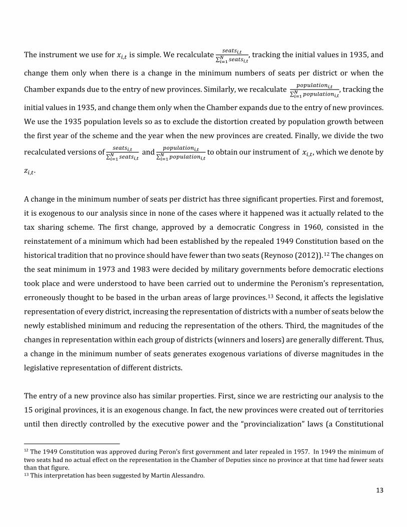
The instrument we use for 𝑥𝑥𝑝𝑝,𝑡𝑡 is simple. We recalculate 𝑡𝑡𝑡𝑡𝑡𝑡𝑡𝑡𝑡𝑡𝑖𝑖,𝑡𝑡∑ 𝑡𝑡𝑡𝑡𝑡𝑡𝑡𝑡𝑡𝑡𝑖𝑖,𝑡𝑡𝑁𝑁𝑖𝑖=1

, tracking the initial values in 1935, and

change them only when there is a change in the minimum numbers of seats per district or when the

Chamber expands due to the entry of new provinces. Similarly, we recalculate 𝑝𝑝𝑝𝑝𝑝𝑝𝑝𝑝𝑝𝑝𝑡𝑡𝑡𝑡𝑝𝑝𝑝𝑝𝑡𝑡𝑖𝑖,𝑡𝑡∑ 𝑝𝑝𝑝𝑝𝑝𝑝𝑝𝑝𝑝𝑝𝑡𝑡𝑡𝑡𝑝𝑝𝑝𝑝𝑡𝑡𝑖𝑖,𝑡𝑡𝑁𝑁𝑖𝑖=1

, tracking the

initial values in 1935, and change them only when the Chamber expands due to the entry of new provinces.

We use the 1935 population levels so as to exclude the distortion created by population growth between

the first year of the scheme and the year when the new provinces are created. Finally, we divide the two

recalculated versions of 𝑡𝑡𝑡𝑡𝑡𝑡𝑡𝑡𝑡𝑡𝑖𝑖,𝑡𝑡∑ 𝑡𝑡𝑡𝑡𝑡𝑡𝑡𝑡𝑡𝑡𝑖𝑖,𝑡𝑡𝑁𝑁𝑖𝑖=1

and 𝑝𝑝𝑝𝑝𝑝𝑝𝑝𝑝𝑝𝑝𝑡𝑡𝑡𝑡𝑝𝑝𝑝𝑝𝑡𝑡𝑖𝑖,𝑡𝑡∑ 𝑝𝑝𝑝𝑝𝑝𝑝𝑝𝑝𝑝𝑝𝑡𝑡𝑡𝑡𝑝𝑝𝑝𝑝𝑡𝑡𝑖𝑖,𝑡𝑡𝑁𝑁𝑖𝑖=1

to obtain our instrument of 𝑥𝑥𝑝𝑝,𝑡𝑡, which we denote by

𝑧𝑧𝑝𝑝,𝑡𝑡.

A change in the minimum number of seats per district has three significant properties. First and foremost,

it is exogenous to our analysis since in none of the cases where it happened was it actually related to the

tax sharing scheme. The first change, approved by a democratic Congress in 1960, consisted in the

reinstatement of a minimum which had been established by the repealed 1949 Constitution based on the

historical tradition that no province should have fewer than two seats (Reynoso (2012)).12 The changes on

the seat minimum in 1973 and 1983 were decided by military governments before democratic elections

took place and were understood to have been carried out to undermine the Peronism’s representation,

erroneously thought to be based in the urban areas of large provinces.13 Second, it affects the legislative

representation of every district, increasing the representation of districts with a number of seats below the

newly established minimum and reducing the representation of the others. Third, the magnitudes of the

changes in representation within each group of districts (winners and losers) are generally different. Thus,

a change in the minimum number of seats generates exogenous variations of diverse magnitudes in the

legislative representation of different districts.

The entry of a new province also has similar properties. First, since we are restricting our analysis to the

15 original provinces, it is an exogenous change. In fact, the new provinces were created out of territories

until then directly controlled by the executive power and the “provincialization” laws (a Constitutional

12 The 1949 Constitution was approved during Peron’s first government and later repealed in 1957. In 1949 the minimum of two seats had no actual effect on the representation in the Chamber of Deputies since no province at that time had fewer seats than that figure. 13 This interpretation has been suggested by Martin Alessandro.

13

requirement) were proposed to the Congress by the executive power and approved by unanimity. Second,

the entry of new provinces affects the legislative representation of every district. In particular, if the new

province obtains a number of seats relative to its population that is higher (lower) than the national pre-

entry ratio, the legislative representation of all the older provinces decreases (increases). Third, although

the direction of the change is the same for every older province, the magnitude of the changes are generally

different. Thus, the entry of a new province also generates exogenous variations of varying magnitudes in

the levels of legislative representation of the different districts.14

Finally, in our analysis we also exploit the political volatility of the country throughout the years covered

in our database; between 1935 and 2011, there were five separate military regimes that lasted from two

to seven years. Given the complete absence of an independent legislative power –the locus of

malapportionment- during military governments, each change in the political regime (from democracy to

military dictatorship or vice versa) produced a radical variation in the extent of legislative representation.

As Potash (1969) (1980) (1996) points out in his detailed work on the Argentine army, in none of the coups

was legislative malapportionment or the tax sharing system an issue and, thus, we can regard these

variations as exogenous for the purpose of our analysis. We use the changes in the political regime to

estimate whether military governments tend to increase (decrease) their transfers to previously

underrepresented (overrepresented) districts, at least partially reverting the biases in the tax revenue

transfers. The 1943 coup -the first one in our sample- was triggered by the efforts of the civil government

to exploit the military for partisan purposes and foreign policy considerations relating to the ongoing world

war. The 1955, 1962 and 1966 coups were all related to Peronism. The Peronist movement significantly

altered the political equilibrium in favor of the working class and against the interests of the land owner

aristocracy which had clear sympathies with the armed forces. Peronism had broad support across the

country so this was predominantly a class conflict rather than a geographical one. Lastly, the 1976 coup

came in the middle of a deep socio political crisis triggered, on the one hand, by the failure of the import

substitution industrialization Argentina had been carrying on since the 1930s and, on the other hand, by

the internal conflict between left wing and right wing Peronists.

14 An example of an endogenous change in legislative representation is a change in the number of seats that is associated with the publication of census results, which, of course, are clearly a reflection of changes in the size of the population of each district.

14

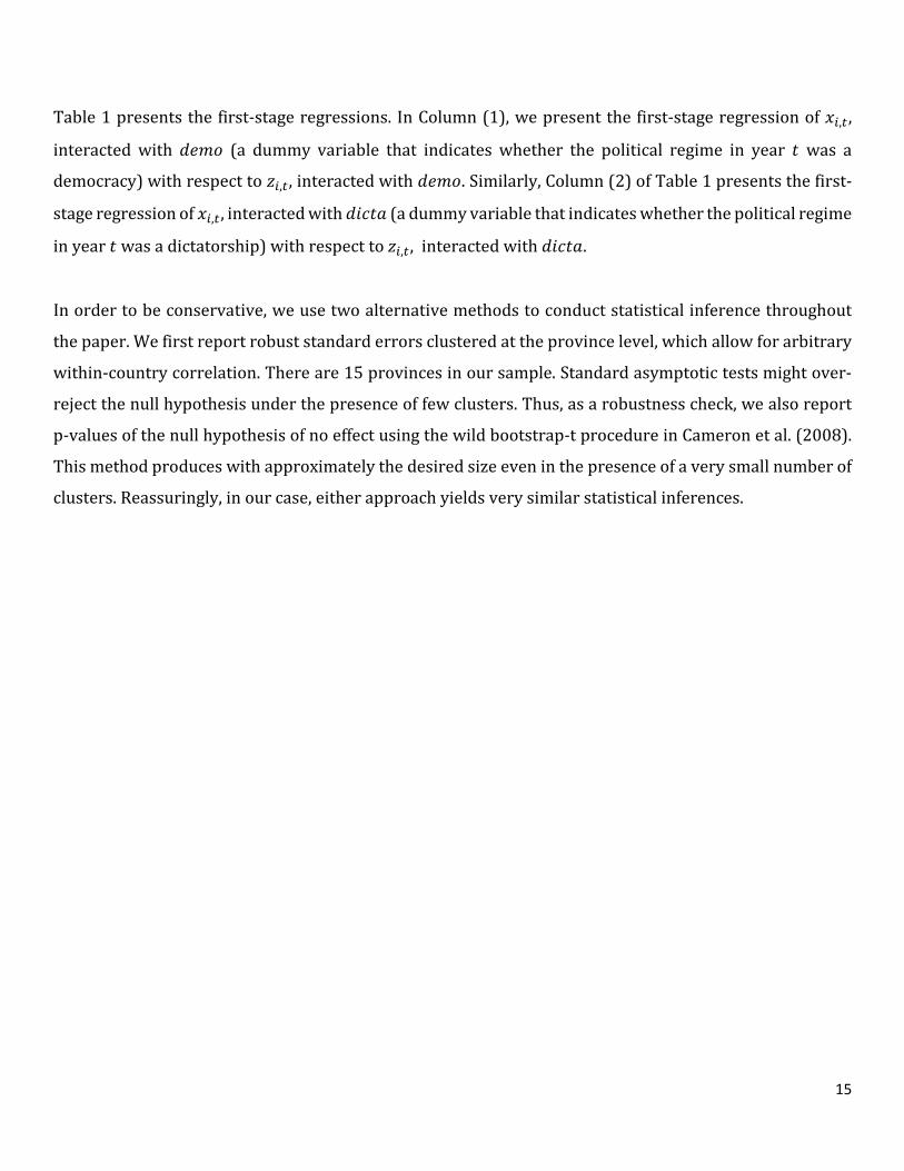
Table 1 presents the first-stage regressions. In Column (1), we present the first-stage regression of 𝑥𝑥𝑝𝑝,𝑡𝑡,

interacted with 𝑑𝑑𝑡𝑡𝑑𝑑𝑝𝑝 (a dummy variable that indicates whether the political regime in year 𝑡𝑡 was a

democracy) with respect to 𝑧𝑧𝑝𝑝,𝑡𝑡, interacted with 𝑑𝑑𝑡𝑡𝑑𝑑𝑝𝑝. Similarly, Column (2) of Table 1 presents the first-

stage regression of 𝑥𝑥𝑝𝑝,𝑡𝑡, interacted with 𝑑𝑑𝑖𝑖𝑑𝑑𝑡𝑡𝑡𝑡 (a dummy variable that indicates whether the political regime

in year 𝑡𝑡 was a dictatorship) with respect to 𝑧𝑧𝑝𝑝,𝑡𝑡, interacted with 𝑑𝑑𝑖𝑖𝑑𝑑𝑡𝑡𝑡𝑡.

In order to be conservative, we use two alternative methods to conduct statistical inference throughout

the paper. We first report robust standard errors clustered at the province level, which allow for arbitrary

within-country correlation. There are 15 provinces in our sample. Standard asymptotic tests might over-

reject the null hypothesis under the presence of few clusters. Thus, as a robustness check, we also report

p-values of the null hypothesis of no effect using the wild bootstrap-t procedure in Cameron et al. (2008).

This method produces with approximately the desired size even in the presence of a very small number of

clusters. Reassuringly, in our case, either approach yields very similar statistical inferences.

15

Table 1: First-Stage Regression

Dependent Variable All Provinces Excluding the

City of Buenos Aires

𝑥𝑥𝑝𝑝,𝑡𝑡 ∗ 𝑑𝑑𝑡𝑡𝑑𝑑𝑝𝑝

(1) 𝑥𝑥𝑝𝑝,𝑡𝑡 ∗ 𝑑𝑑𝑖𝑖𝑑𝑑𝑡𝑡𝑡𝑡 (2) 𝑥𝑥𝑝𝑝,𝑡𝑡 ∗ 𝑑𝑑𝑡𝑡𝑑𝑑𝑝𝑝

(3) 𝑥𝑥𝑝𝑝,𝑡𝑡 ∗ 𝑑𝑑𝑖𝑖𝑑𝑑𝑡𝑡𝑡𝑡 (4)

𝑧𝑧𝑝𝑝,𝑡𝑡 ∗ 𝑑𝑑𝑡𝑡𝑑𝑑𝑝𝑝 0.986*** -0.003 0.972*** -0.037

(0.121) [0.008]

(0.094) [0.928]

(0.121) [0.008]

(0.090) [0.644]

𝑧𝑧𝑝𝑝,𝑡𝑡 ∗ 𝑑𝑑𝑖𝑖𝑑𝑑𝑡𝑡𝑡𝑡 0.140*** 1.003*** 0.107** 0.978***

(0.050) [0.008]

(0.098) [0.000]

(0.049) [0.036]

(0.097) [0.000]

F-Test 66.83 97.79 64.02 96.43 Observations 1155 1155 1078 1078 Note: All regressions include year effects, province effects and province linear trends. These regressors are partialled out in the estimation.15 Province-clustered standard errors in parentheses; Wild clustered bootstrap p-values for t-statistics computed as proposed by Cameron et al. (2008) in italics. * significantly different from zero at 10%, ** at 5%, *** at 1%.

Note that the coefficients corresponding to the instruments in Table 1 are all statistically significant at the

1 percent level. More importantly, it is clear that only the variability in 𝑧𝑧𝑝𝑝,𝑡𝑡 is exogenous and that this

exogenous variability it is not correlated with other variability in legislative malapportionment such as

that induced by population change. The fact that the coefficient of 𝑧𝑧𝑝𝑝,𝑡𝑡 is very close to one indicates that the

variability of the instrumented variable will practically mimick that of the instrument, thus reassuring us

that we are only relying on exogenous variations for the purpose of our analysis. Therefore, our

instrumental variable approach is fundamental to obtain consistent estimates of the effects of legislative

malapportionment on federal tax transfers.

4.1. Regression Model

We estimate the following model:

𝑦𝑦𝑝𝑝,𝑡𝑡 = β1 ∗ 𝑥𝑥𝑝𝑝,𝑡𝑡 ∗ 𝑑𝑑𝑖𝑖𝑑𝑑𝑡𝑡𝑡𝑡t + β2 ∗ 𝑥𝑥𝑝𝑝,𝑡𝑡 ∗ 𝑑𝑑𝑡𝑡𝑑𝑑𝑝𝑝 t + δi + λt + μi ∗ 𝑝𝑝𝑡𝑡𝑝𝑝𝑝𝑝𝑡𝑡𝑡𝑡𝑡𝑡𝑡𝑡𝑑𝑑 + εi,t (5.)

15 See Baum, Schaffer and S. Stillman (2007).

16

where 𝑑𝑑𝑡𝑡𝑑𝑑𝑝𝑝 (𝑑𝑑𝑖𝑖𝑑𝑑𝑡𝑡𝑡𝑡) is a dummy variable that indicates whether the political regime in year 𝑡𝑡 was a

democracy (dictatorship) or not, δi and λt are province and year effects, respectively, and 𝑝𝑝𝑡𝑡𝑝𝑝𝑝𝑝𝑡𝑡𝑡𝑡𝑡𝑡𝑡𝑡𝑑𝑑 is a

province-specific linear trend.

Several remarks about this specification apply. First, we estimate this model for the 15 original districts in

the scheme. Second, the standard malapportionment theory would predict a positive sign for β2. The higher

the 𝑥𝑥𝑝𝑝,𝑡𝑡 of the district, the more represented the district is relative to other districts and, hence, the more

transfers per inhabitant relative to the average transfer per inhabitant it can be expected to receive. Under

non-democratic regimes, we calculate 𝑥𝑥𝑝𝑝,𝑡𝑡 using the seat distribution in the latest session of Congress.

Therefore, the standard malapportionment theory would suggest a negative sign for β1. Given the absence

of legislative malapportionment in military governments, we would expect that they try to shift the tax

sharing scheme toward a less biased distribution. Thus, the higher the 𝑥𝑥𝑝𝑝,𝑡𝑡 of a district in a non-democratic

period, the better represented the district would have been in the previous democratic period and the more

funds it can be expected to receive now.

5. Main Results

Table 2 presents the main results. Note that the coefficients associated with 𝑥𝑥𝑝𝑝,𝑡𝑡 ∗ 𝑑𝑑𝑖𝑖𝑑𝑑𝑡𝑡𝑡𝑡 and 𝑥𝑥𝑝𝑝,𝑡𝑡 ∗ 𝑑𝑑𝑡𝑡𝑑𝑑𝑝𝑝 are

statistically significant when they are not instrumented by 𝑧𝑧𝑝𝑝,𝑡𝑡 ∗ 𝑑𝑑𝑖𝑖𝑑𝑑𝑡𝑡𝑡𝑡 and 𝑧𝑧𝑝𝑝,𝑡𝑡 ∗ 𝑑𝑑𝑡𝑡𝑑𝑑𝑝𝑝 (column 1). However,

once 𝑥𝑥𝑝𝑝,𝑡𝑡 ∗ 𝑑𝑑𝑖𝑖𝑑𝑑𝑡𝑡𝑡𝑡 and 𝑥𝑥𝑝𝑝,𝑡𝑡 ∗ 𝑑𝑑𝑡𝑡𝑑𝑑𝑝𝑝 are instrumented by 𝑧𝑧𝑝𝑝,𝑡𝑡 ∗ 𝑑𝑑𝑖𝑖𝑑𝑑𝑡𝑡𝑡𝑡 and 𝑧𝑧𝑝𝑝,𝑡𝑡 ∗ 𝑑𝑑𝑡𝑡𝑑𝑑𝑝𝑝, the coefficients drop

steeply toward zero and are not statistically significant (column 3). Indeed, the 2SLS point estimates are

very small and also economically insignificant.

17

Table 2: Main Results

Instrumental Variable Regressions

All

Provinces

Excluding the City of

Buenos Aires All

Provinces

Excluding the City of

Buenos Aires (1) (2) (3) (4)

𝑥𝑥𝑝𝑝,𝑡𝑡 ∗ 𝑑𝑑𝑖𝑖𝑑𝑑𝑡𝑡𝑡𝑡 0.498*** 0.491*** 0.166 0.113 (0.141) (0.159) (0.188) (0.201) [0.064] [0.088] [0.464] [0.612] 𝑥𝑥𝑝𝑝,𝑡𝑡 ∗ 𝑑𝑑𝑡𝑡𝑑𝑑𝑝𝑝 0.513*** 0.495*** 0.102 0.031 (0.135) (0.152) (0.208) (0.220) [0.044] [0.056] [0.608] [0.848] F-Test (Kleinberg-Paap) 42.88 45.12 Observations 1155 1078 1155 1078 Note: All regressions include year effects, province effects and province linear trends. These regressors are partialled out in the IV estimation. Province-clustered standard errors are shown in parentheses; * significantly different from zero at 10%, ** at 5%, *** at 1%. Wild clustered bootstrap p-values for t-statistics computed as proposed by Cameron et al. (2008) in italics.

In line with the standard malapportionment hypothesis, Table 2 column (1) shows a positive correlation

between the legislative representation of a district and the per capita transfers received by the district

(both expressed as a ratio with respect to the total country value) in democratic periods. Contrary to the

standard malapportionment hypothesis, Table 2 column (1) shows that this positive correlation persists

under centralized military governments. Table 2 column (3) brings to the forefront the problems of

interpreting these correlations as causal relationships. Indeed, once we instrument 𝑥𝑥𝑝𝑝,𝑡𝑡 ∗ 𝑑𝑑𝑖𝑖𝑑𝑑𝑡𝑡𝑡𝑡 and 𝑥𝑥𝑝𝑝,𝑡𝑡 ∗

𝑑𝑑𝑡𝑡𝑑𝑑𝑝𝑝 with 𝑧𝑧𝑝𝑝,𝑡𝑡 ∗ 𝑑𝑑𝑖𝑖𝑑𝑑𝑡𝑡𝑡𝑡 and 𝑧𝑧𝑝𝑝,𝑡𝑡 ∗ 𝑑𝑑𝑡𝑡𝑑𝑑𝑝𝑝, respectively, the coefficients drop toward zero and they are not

statistically significant.

Although we have shown that there is no robust statistical evidence that legislative malapportionment has

a causal effect on the distribution of federal tax revenues, the positive correlation in Table (2) column (1)

is intriguing. One potential explanation is that this correlation captures the endogenous relationship

between legislative representation and the distribution of tax revenues that emerge from the country’s

deep-seated political equilibrium. For example, as the power of a province in the informal bargaining

18

process over fiscal revenues increases, the legislative representation and the funds received by the

province might also increase. The subtle point is that the increase in legislative representation is not

valuable because it enhances the power of the district in the legislature, thus increasing the likelihood of

future transfers. On the contrary, legislative representation has a value in itself as a rent for local

politicians. This may also explain the positive correlation between legislative representation in the last

democratic Congress and transfers received under centralized military governments. The districts that

were increasing their political power or becoming easier to please by the president before the coup, were

receiving more transfers and more political representation. The same districts continued receiving more

transfers after the coup because the autocrat must also take into account in his political calculus that it is

easier to grant the support of these districts.

One issue of concern in relation to the results in column (3) of Table 2 may be the potentially spurious

effect created by outliers such as the City of Buenos Aires, which is a district that has been overrepresented

since the late 1980s and, at the same time, receives a very small portion of tax revenues. This negative

effect of overrepresentation may potentially balance out a positive effect seen in other provinces and,

therefore, lead to a non-significant overall effect such as the one that is shown in our results. We re-

estimate our main regressions after excluding the City of Buenos Aires from our sample. As columns (2)

and (4) in Table 2 show, the results do not change.

Another potential concern is that when the federal tax sharing scheme was put in place in 1935, some

provinces depended heavily on domestic tax receipts. To accommodate this situation and to avoid

disrupting these provinces’ budgets, the law provided for a transitional period in which these provinces

would have a special status and receive a considerable share of total revenues. In order to factor out any

bias that might be generated by this transitional period, we re-estimated our regressions while excluding

the observations for the first years of the tax sharing scheme (1935-1940). The results did not change.16

To sum up, overall there is no robust statistical evidence to back up the argument that legislative

malapportionment has a causal effect on the distribution of federal tax revenues. Moreover, there is no

16 The coefficients of 𝑥𝑥𝑝𝑝,𝑡𝑡 ∗ 𝑑𝑑𝑖𝑖𝑑𝑑𝑡𝑡𝑡𝑡 and 𝑥𝑥𝑝𝑝,𝑡𝑡 ∗ 𝑑𝑑𝑖𝑖𝑑𝑑𝑡𝑡𝑡𝑡 are 0.373 and 0.497, respectively. The first one is statistically significant at 5%, while the second is statistically significant at 1%. However, once 𝑥𝑥𝑝𝑝,𝑡𝑡 ∗ 𝑑𝑑𝑖𝑖𝑑𝑑𝑡𝑡𝑡𝑡 and 𝑥𝑥𝑝𝑝,𝑡𝑡 ∗ 𝑑𝑑𝑖𝑖𝑑𝑑𝑡𝑡𝑡𝑡 are instrumented by 𝑧𝑧𝑝𝑝,𝑡𝑡 ∗ 𝑑𝑑𝑖𝑖𝑑𝑑𝑡𝑡𝑡𝑡 and 𝑧𝑧𝑝𝑝,𝑡𝑡 ∗ 𝑑𝑑𝑡𝑡𝑑𝑑𝑝𝑝, the coefficients are not statistically significant.

19

evidence to support the thesis that, under centralized military governments, the tax sharing arrangement

reverted to a less biased distribution because of the absence of malapportionment.

6. A Simple Model

In this section we develop a very simple politico-economic model of a tax sharing system. We show that a

democracy with a dominant executive branch and an autocracy can generate the same shares for each

district, while a democracy with a powerful, malapportioned Congress induces a bias toward

overrepresented districts. The model provides some theoretical foundations for our empirical results.

6.1 The Economy

Consider an economy that is made up of two districts indexed by 𝑗𝑗 = 1, 2. Each district is home to two

socioeconomic groups, the poor and the rich, which are indexed by 𝑖𝑖 = 𝑃𝑃,𝑅𝑅. The population in district 𝑗𝑗 is

𝑁𝑁𝑗𝑗 , and we normalize 𝑁𝑁1 + 𝑁𝑁2 = 1. The proportion of poor agents in each district is 𝑡𝑡𝑃𝑃. Denote by 𝑦𝑦𝑝𝑝𝑗𝑗 the

income of a member of socioeconomic group 𝑖𝑖 in district 𝑗𝑗 and assume that rich (poor) people in district 1

are wealthier than rich (poor) people in district 2. Specifically, assume 𝑦𝑦𝑅𝑅1 = (1 + 𝛽𝛽)𝑦𝑦𝑅𝑅2 and 𝑦𝑦𝑃𝑃1 = (1 + 𝛾𝛾)𝑦𝑦𝑃𝑃2,

where 0 < 𝛽𝛽 < 𝛾𝛾 < 𝑦𝑦𝑅𝑅2−𝑦𝑦𝑃𝑃

2

𝑦𝑦𝑃𝑃2 . 𝛽𝛽 > 0 and 𝛾𝛾 > 0 assures that district 1 is richer than district 2; 𝛽𝛽 < 𝛾𝛾 implies

that the level of inequality is lower in district 1 than in district 2; and 𝛾𝛾 < 𝑦𝑦𝑅𝑅2−𝑦𝑦𝑃𝑃

2

𝑦𝑦𝑃𝑃2 implies that rich agents in

district 2 are richer than poor agents in district 1.

We assume that there are four goods: a private good (𝑑𝑑𝑝𝑝𝑗𝑗), one national public good (𝑔𝑔), and two local public

goods (𝑔𝑔1 and 𝑔𝑔2). Public goods are financed by a proportional income tax (𝜏𝜏). As a consequence, the

individual budget constraint is simply:

𝑑𝑑𝑝𝑝𝑗𝑗 = (1 − 𝜏𝜏)𝑦𝑦𝑝𝑝

𝑗𝑗 (6.)

and the government budget constraint is given by:

𝜏𝜏𝑦𝑦 = 𝑔𝑔 + 𝑔𝑔1 + 𝑔𝑔2 (7.)

20

where 𝑦𝑦 = 𝑡𝑡𝑃𝑃(1 + 𝛾𝛾𝑁𝑁1)𝑦𝑦𝑃𝑃2 + (1 − 𝑡𝑡𝑃𝑃)(1 + 𝛽𝛽𝑁𝑁1)𝑦𝑦𝑅𝑅2 is the aggregate income.

Agents value the private good, the national public good, and the local public goods in their district.

Specifically, for 𝑖𝑖 = 𝑃𝑃,𝑅𝑅 and 𝑗𝑗 = 1, 2 and, after introducing the individual and government budget

constraints, we have:

𝑝𝑝𝑝𝑝𝑗𝑗(𝑔𝑔,𝑔𝑔1,𝑔𝑔2) = �1 −

𝑔𝑔 + 𝑔𝑔1 + 𝑔𝑔2

𝑦𝑦�𝑦𝑦𝑝𝑝

𝑗𝑗 + 𝐻𝐻�𝑔𝑔,𝑔𝑔𝑗𝑗� (8.)

where 𝐻𝐻�𝑔𝑔,𝑔𝑔𝑗𝑗� is strictly quasi-concave and satisfies the Inada conditions. For example,

𝐻𝐻�𝑔𝑔,𝑔𝑔𝑗𝑗� = 𝛼𝛼(𝑔𝑔)1−𝜎𝜎

1 − 𝜎𝜎+ (1 − 𝛼𝛼)

�𝑔𝑔𝑗𝑗�1−𝜐𝜐

1 − 𝜐𝜐, 𝑖𝑖𝑡𝑡 𝜎𝜎 ≠ 1 𝑡𝑡𝑡𝑡𝑑𝑑 𝜐𝜐 ≠ 1 (9.)

6.2 The Polity

We consider two possible political regimes: democracy and autocracy. Following Acemoglu and Robinson

(2006), we assume that, under democracy, the government represents the poor people, i.e., it maximizes a

social welfare function that only gives weight to the welfare of the two poor groups.17 More formally:

max(𝜏𝜏,𝑔𝑔,𝑔𝑔1,𝑔𝑔2)

�𝑊𝑊(𝐷𝐷) = 𝑡𝑡𝑃𝑃�𝜔𝜔1(𝐷𝐷)𝑝𝑝𝑃𝑃1 + �1 − 𝜔𝜔1(𝐷𝐷)�𝑝𝑝𝑃𝑃2�� (10.)

where 𝜔𝜔1(𝐷𝐷) = 𝑁𝑁1𝜑𝜑1

𝑁𝑁1𝜑𝜑1+1−𝑁𝑁1< 1 and 𝜑𝜑1 > 0. For a democracy in which the executive branch predominates

over the legislature or where there is no malapportionment in the legislature, the government assigns

weights to each poor group solely on the basis of its size, i.e., 𝜑𝜑1 = 1. For a democracy in which the

legislature wields power and there is malapportionment, then 𝜑𝜑1 > 1 if district 1 is overrepresented and

𝜑𝜑1 < 1 if district 1 is underrepresented.

17 It is possible to build a detailed electoral model that leads to this welfare function. For example, we can employ a probabilistic voting model (Grossman and Helpman 2001).

21

Under an autocracy, the government represents the rich groups, i.e., it maximizes a social welfare function

that assigns weights only to the welfare of the two rich groups.18 More formally,

max(𝜏𝜏,𝑔𝑔,𝑔𝑔1,𝑔𝑔2)

�𝑊𝑊(𝐴𝐴) = (1 − 𝑡𝑡𝑃𝑃)�𝜔𝜔1(𝐴𝐴)𝑝𝑝𝑅𝑅1 + �1 − 𝜔𝜔1(𝐴𝐴)�𝑝𝑝𝑅𝑅2�� (11.)

where 𝜔𝜔1(𝐴𝐴) = 𝑁𝑁1 < 1.

6.3 Fiscal Policy under Different Political Regimes

Denote by �𝑔𝑔(𝑅𝑅𝑅𝑅𝐺𝐺),𝑔𝑔1(𝑅𝑅𝑅𝑅𝐺𝐺),𝑔𝑔2(𝑅𝑅𝑅𝑅𝐺𝐺)� the allocation of public goods under political regime 𝑅𝑅𝑅𝑅𝐺𝐺 =

{𝐷𝐷,𝐴𝐴}, where 𝐷𝐷 is a democracy and 𝐴𝐴 is an autocracy. Denote by 𝑡𝑡𝑗𝑗(𝑅𝑅𝑅𝑅𝐺𝐺) the share of each district of the

resources that finance local public goods and by 𝑡𝑡𝐹𝐹(𝑅𝑅𝑅𝑅𝐺𝐺) the share of the federal government. Then:

𝑡𝑡𝑗𝑗(𝑅𝑅𝑅𝑅𝐺𝐺) =𝑔𝑔𝑗𝑗(𝑅𝑅𝑅𝑅𝐺𝐺)

𝑔𝑔1(𝑅𝑅𝑅𝑅𝐺𝐺) + 𝑔𝑔2(𝑅𝑅𝑅𝑅𝐺𝐺) , 𝑡𝑡𝐹𝐹(𝑅𝑅𝑅𝑅𝐺𝐺) =𝑔𝑔(𝑅𝑅𝑅𝑅𝐺𝐺)

𝑔𝑔1(𝑅𝑅𝑅𝑅𝐺𝐺) + 𝑔𝑔2(𝑅𝑅𝑅𝑅𝐺𝐺) + 𝑔𝑔(𝑅𝑅𝑅𝑅𝐺𝐺) (12.)

The following proposition characterizes fiscal policy under different political regimes.

Proposition 1: Suppose that 𝐻𝐻2�𝑔𝑔, 𝜆𝜆𝑔𝑔𝑗𝑗� = 𝜆𝜆𝜃𝜃𝐻𝐻2�𝑔𝑔,𝑔𝑔𝑗𝑗� for some 𝜃𝜃 < 0 and every 𝜆𝜆 > 0. Then, the revenue

share of each local district under a democracy with a dominant executive branch or in which there is no

legislative malapportionment will be the same as under an autocracy. Moreover, the overrepresented district

under a democracy not dominated by the Executive will obtain a larger share of the revenues than it will under

an autocracy. Formally:

𝑡𝑡1(𝐷𝐷)(𝜑𝜑1 < 1) < 𝑡𝑡1(𝐷𝐷)(𝜑𝜑1 = 1) = 𝑡𝑡1(𝐴𝐴) < 𝑡𝑡1(𝐷𝐷)(𝜑𝜑1 > 1) (13.)

Proof: See Appendix B. ∎

Formally, Propositions 1 give a conditions for preferences under which the distribution of tax revenues

among the districts does not vary with the political regime. Conceptually, Proposition 1 shows that military

18 The welfare function can be the outcome of a bargaining process between the two rich groups.

22

coups may not affect the distribution of tax revenues among districts in countries with a strong executive

branch during periods when a democratic system of government is in power. In other words, changes in

the political regime can modify the distribution between the poor and the rich without affecting the relative

position of different districts.

So far, we have implicitly assumed that an autocracy assigns the same weight to a rich person regardless

of his or her location. Analogously, a democracy dominated by the executive branch assigns the same

weight to every poor citizen. Of course, this is not necessarily the case. For example, in some districts,

patronage could be more likely to occur. The key point is, however, that the districts whose support is

easier for a strong president in a democratic system to buy are probably also the same districts that will be

more willing to sell their support to military governments. The supposition that democracies represent a

coalition of poor citizens and autocracies represent a coalition of rich people does not imply that

democracies and autocracies produce a different geographic pattern of representation. As a consequence,

changes in the political regime can be associated with changeovers in policy that may have a significant

effect on the relative well-being of poor and rich people without producing any major change in the shares

of resources obtained by each jurisdiction. Thus, biases in the geographic distribution of resources can

persist in the absence of a strong Congress because an autocrat that represents the rich must deal with

more or less the same political constraints between districts as a dominant Executive that represents the

poor19. Formally, we can rework Proposition 1 with 𝜔𝜔1(𝐷𝐷) = 𝑁𝑁1�𝜑𝜑1+𝜇𝜇1�𝑁𝑁1(𝜑𝜑1+𝜇𝜇1)+1−𝑁𝑁1

and 𝜔𝜔1(𝐴𝐴) = 𝑁𝑁1𝜇𝜇1

𝑁𝑁1𝜇𝜇1+1−𝑁𝑁1, where

𝜇𝜇1 is a measure of the overrepresentation (when 𝜇𝜇1 > 1) or sub-representation (when 𝜇𝜇1 < 1) of district

1 that is unrelated to legislative malapportionment. It is easy to show that analogous results will be

obtained.

19 A military government once tried to exclude a district from the sharing scheme –the city of Buenos Aires in 1981- but had to reverse its decision two years later, showing in fact the difficulty in altering the equilibrium.

23

7. Why Is Legislative Malapportionment Immaterial in Argentina?

As we have shown in Section 5, we cannot attribute the biases in the tax sharing system to

malapportionment during democratic periods. Why have changes in legislative malapportionment had no

effect on the shares of the different provinces? The model we have developed in Section 6 suggests that, in

democracies dominated by the executive branch, legislative malapportionment is not very relevant. In

Section 5, we have also shown that military governments did not reverse the distribution of federal tax

revenues among the provinces. Since military governments closed the Congress and concentrated

legislative power in their own hands, this result also deserves a more detailed explanation. Why did biased

distributions persist under non-democratic regimes? The model we have developed in Section 6 suggests

that geographic representation may not be very sensitive to the type of political regime that is in place. In

this section we further explore these questions.

7.1. Legislator Behavior, Party Discipline and Parliamentary Coalitions

A necessary condition in order for changes in malapportionment to have an effect on policy outcomes is

the existence of a correlation between legislator behavior and the preferences of the constituents whom

they represent at the district level. If party discipline is strong, then the geographic origin of legislators

may not be relevant, since their party affiliation is what will matter the most.

The evidence, however, shows that legislators respond to subnational interests, although in very different

ways. Members of the U.S. Congress exhibit a great deal of autonomy in choosing whether or not to follow

the party line on many issues, as Snyder and Groseclose (2000) show. Only on national issues such as the

debt ceiling, tax policy and budget resolutions is the vote mostly partisan. On issues which usually have a

clear geographic dimension, such as transportation, public works or agriculture, the party whip wields

much less power. The main reason for such behavior may be that U.S. legislators are very responsive to

electoral incentives at the constituency level because of the uninominal nature of congressional districts.

Concerning the case of Japan, Kato (1998) analyzes the split of the Liberal Democratic Party in 1993 and

shows that legislators with local support bases tended to be part of the “rebel” group that separated from

the party at that time.

24

Jones et al. (2002) analyze the situation in Argentina and show that the link between subnational interests

and legislators’ behavior is mediated by the fact that deputies are generally beholden to provincial

governors. Unlike the situation in the U.S., a seat in Congress is seen as a temporary stage in a person’s

political career. Indeed, most of the Argentine legislators remain in office for only one term: the reelection

rate in the Chamber of Deputies is around 20%. The careers of Argentine politicians are mostly province-

based and, as a result, legislators in Congress will tend to cater to the regional interests espoused by local

party bosses – especially governors. As Levitsky’s work (2003) has shown, this “territorialization” of

political incentives is clearly discernible in the most important party in Argentina – the Peronist (or

“Justicialista”) Party, which has governed Argentina during most of its periods of democracy since 1945.

A more subtle condition that is required in order for changes in malapportionment to have a significant

effect on the pattern of policy biases is that the changes must be large enough to destabilize the majority

coalition in Congress. For example, we could attribute the key biases of the Argentine tax sharing system

to the existence of a majority congressional coalition composed of poor provinces that have won out over

the richer Buenos Aires Province and capital district. Although the changes in the degree of legislative

malapportionment that have occurred during the existence of the tax sharing system have probably not

been dramatic enough to pose a challenge to this majority coalition, it is more difficult to argue convincingly

that the observed changes in legislative malapportionment have not been large enough to at least modify

the distribution of revenues among the members of that coalition. And yet, our results show that legislative

malapportionment has had no causal impact on the shares received by the various provinces.

7.2. The Predominance of the Executive Branch

A more compelling hypothesis to explain why legislative malapportionment does not matter is that, in

Argentina, key political decisions are the outcome of a bargaining process among executive authorities --

more specifically, between the president and the governors. In fact, Braun and Tommasi (2002) document

the fact that legislative representation of subnational entities in Argentina is relatively poor and that the

relationship between the central government and the provinces is scarcely institutionalized at all and

instead consists mainly in a direct dialogue between the national executive authority (the president) and

the provincial executives (the governors). In other words, Congress is not the locus of bargaining and, by

the time a bill reaches Congress, it has already been discussed with the governors. As a consequence, there

25

is no need to form a coalition to give expression to provincial interests in Congress because the preferences

of the provinces have already been taken into account.

The predominance of the Argentine executive branch can be traced back to a variety of factors. For

example, on several occasions, the Argentine Congress has delegated part of its legislative authority to the

executive branch. National legislators frequently leave their seats in order to become part of the executive

branch or to run for office at a local level, implicitly revealing their assessment of the relative importance

of a seat in Congress vis-à-vis a position in a ministry or the possibility of running for mayor. Even in the

case where a president has resigned, political power rests with the governors of the provinces rather than

with Congress. In point of fact, in 2001, during a profound economic and political crisis, the president of

Argentina did resign. Although, nominally, Congress was in charge of designating a new president, the

actual bargaining involved in that appointment was carried out among the governors. As it happened,

Congress temporarily selected the governor of San Luis as the president, but, in less than a week, he fell

out of favor with the other governors and was replaced by the governor of Buenos Aires.

7.3. Geographic Representativeness of the Executive Branch

The predominance of the executive branch is potentially a convincing explanation for why legislative

malapportionment does not affect the tax sharing system under democracies in Argentina. The

predominance of the executive branch cannot by itself explain why military governments have not

significantly altered the allocation of revenues among provinces, however. After all, we would tend to

expect that the powers of the executive branch under autocracies and democracies would differ in many

ways. Yet, in Argentina, the geographic representativeness of the federal executive branch does not appear

to change significantly from one political regime to the other.

In order to measure the geographic representativeness of the executive branch, we have created a database

with information on the province of birth of the main members of all the governments between 1935 and

2011.20 For democratic governments, we have gathered information referring to the president, vice-

president, minister of economic affairs and minister of the interior. For military governments, the

20 All the data refer to the members of the government as of June 30th of each year.

26

information corresponds to the military junta21 (the chiefs of the army, the navy and the air force), the

minister of economic affairs and the minister of the interior.

We have used this information to develop an index that quantifies the degree of geographic

representativeness of each government (i.e., how much of the population is actually “represented” in the

executive branch). To this end, we add up the proportions of the population corresponding to the districts

of origin of the above-mentioned government authorities.

Figure 3 shows our index of geographic representation. As can be seen from the graph, there have been

periods when the government has not been very representative in geographical terms. Take, for instance,

1992, when the President and the (acting) Vice-President were both from tiny La Rioja, the Minister of

Economic Affairs was from Córdoba and the Minister of the Interior was from Mendoza. The populations

of those three districts added up to only 13.5% of the population of Argentina. In contrast, in 1979, during

the last military government, the Chief of Staff of the Army was from Buenos Aires Province, the Chief of

Staff of the Navy was from the City of Buenos Aires, the Chief of Staff of the Air Force was from Santa Fe,

the Minister of Economic Affairs was from Salta and the Minister of the Interior was from Córdoba. The

populations of those districts added up to 69.3% of the total national population.

21 Some military governments used formal procedures to choose a president and vice-president. In those cases, the above information corresponds to those two positions.

27

Figure 3: Geographic Representation Index

Note: Shaded areas represent military governments.

Using our index of geographic representation, we can construct a test to see whether military governments

are more representative in geographical terms than democratic ones. In Table 3 we present the results of

an equal means test for democratic and military governments. As can be seen from the table, there is no

statistically significant difference between the mean values on our index for the two types of political

regimes.

Table 3: Equal Means Test Based on the Geographic Representation Index

Democracy Military Government Difference

GRI 0.429 0.474 0.045

(0.115) (0.149) (0.032)

T-test p-value 0.160

Observations 55 22

28

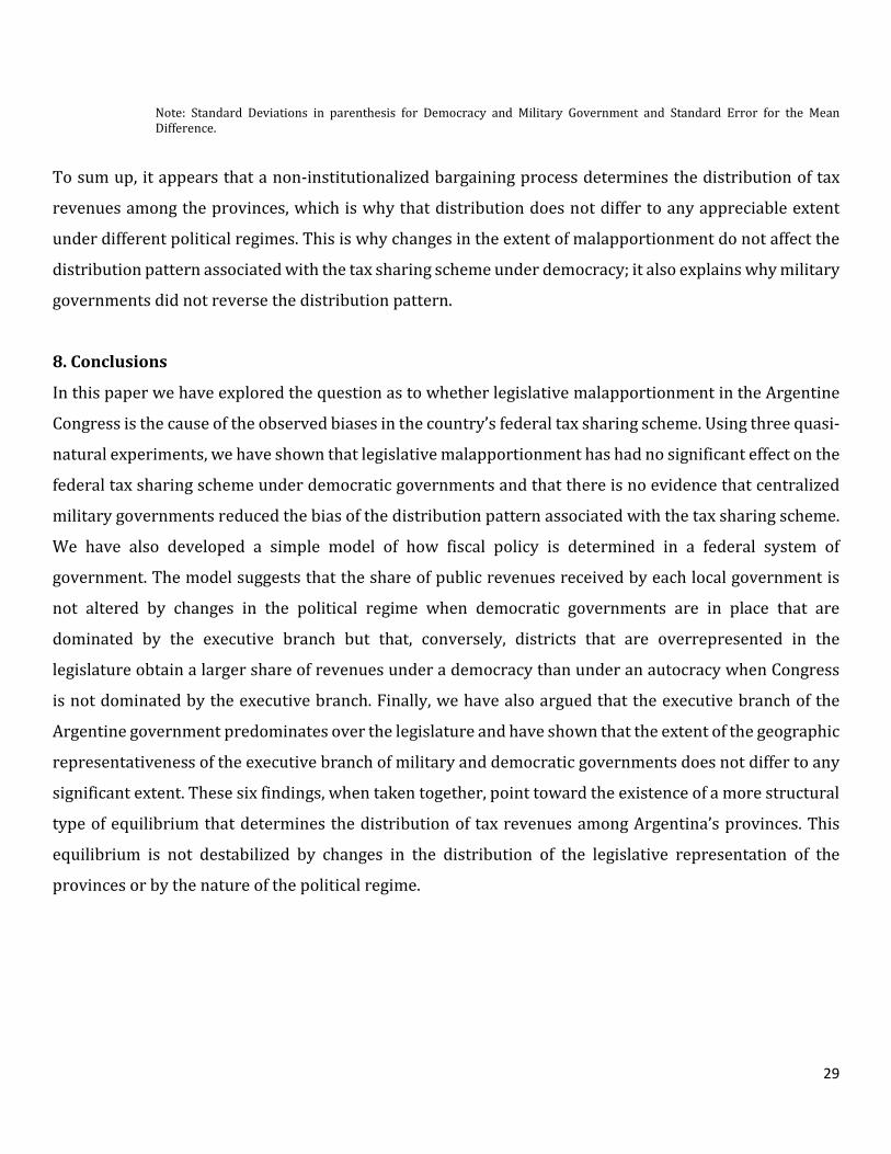
Note: Standard Deviations in parenthesis for Democracy and Military Government and Standard Error for the Mean Difference.

To sum up, it appears that a non-institutionalized bargaining process determines the distribution of tax

revenues among the provinces, which is why that distribution does not differ to any appreciable extent

under different political regimes. This is why changes in the extent of malapportionment do not affect the

distribution pattern associated with the tax sharing scheme under democracy; it also explains why military

governments did not reverse the distribution pattern.

8. Conclusions

In this paper we have explored the question as to whether legislative malapportionment in the Argentine

Congress is the cause of the observed biases in the country’s federal tax sharing scheme. Using three quasi-

natural experiments, we have shown that legislative malapportionment has had no significant effect on the

federal tax sharing scheme under democratic governments and that there is no evidence that centralized

military governments reduced the bias of the distribution pattern associated with the tax sharing scheme.

We have also developed a simple model of how fiscal policy is determined in a federal system of

government. The model suggests that the share of public revenues received by each local government is

not altered by changes in the political regime when democratic governments are in place that are

dominated by the executive branch but that, conversely, districts that are overrepresented in the

legislature obtain a larger share of revenues under a democracy than under an autocracy when Congress

is not dominated by the executive branch. Finally, we have also argued that the executive branch of the

Argentine government predominates over the legislature and have shown that the extent of the geographic

representativeness of the executive branch of military and democratic governments does not differ to any

significant extent. These six findings, when taken together, point toward the existence of a more structural

type of equilibrium that determines the distribution of tax revenues among Argentina’s provinces. This

equilibrium is not destabilized by changes in the distribution of the legislative representation of the

provinces or by the nature of the political regime.

29

References Acemoglu, Daron, and James A. Robinson. 2006. Economic Origins of Dictatorship and Democracy. New York: Cambridge

University Press.

Ansolabehere, Stephen, Alan Gerber, and James M. Snyder. 2002. "Equal Votes, Equal Money: Court-Ordered Redistricting and the Distribution of Public Expenditures in the American State." American Political Science Review 96(4):767-77.

Ansolabehere, Stephen, James M. Snyder, and Michael Ting. 2003. "Bargaining in Bicameral Legislatures: When and Why does malapportionment matter." American Political Science Review 97(3): 471-481.

Baron, David, and John Ferejohn. 1989. "Bargaining in Legislatures." American Political Science Review 83(4):1186-1206.

Baum, Christopher F., Schaffer, Mark E., Stillman, Steven. 2007. "Enhanced Routines for Instrumental Variables/Generalized Method of Moments Estimation and Testing." The Stata Journal 465:506.

Braun, Miguel, and Mariano Tommasi. 2002. "Fiscal Rules for Subnational Governments: Some Organizing Principles and Latin American Experiences." In Rules and Practice in Inter-governmental Fiscal Relations, by G. Kopits (comp.). Washington D.C.: IMF and World Bank, Washington.

Bruhn, Miriam, Francisco Gallego and Massimiliano Onorato. 2010. "Legislative Malapportionment and Institutional Persistence." Policy Research Working Paper 5467, World Bank, Washington D.C.

Dragu, Tiberiu, and Jonathan Rodden. 2011. "Representation and Redistribution in Federations." Proceedings of the National Academy of Science of the United States of America 108(21):8601–8604.

Gibson, Edward, Ernesto Calvo, and Tulia Falleti. 2004. "Reallocative Federalism: Legislative Overrepresentation and Public Spending in the Western Hemisphere." In Federalism and Democracy in Latin America, by E. Gibson (comp.). The Johns Hopkins University.

Gordin, Jorge P. 2010. "Patronage-Preserving Federalism? Legislative Malapportionment and Subnational Fiscal Policies." In Exploring New Avenues in Comparative Federalism, by Erk Jan and Wilfried (comp.) Swenden. London: Routledge.

Grossman, Gene M., and Elhanan Helpman. 2001. Special Interest Politics. Cambridge Massachusetts: MIT Press.

Horiuchi, Yusaku, and Saito Jun. 2003. "Reapportionment and Redistribution: Consequences of Electoral Reform in Japan." American Journal of Political Science 47(4):669-682.

Jones, Mark, Sebastián Saiegh, Pablo Spiller, and Mariano Tommasi. 2002. "Amateur Legislators – Professional Politicians: The Consequences of Party-Centered Electoral Rules in a Federal System." American Journal of Political Science 46(3): 656-669.

Kato, Junko. 1998. "When the Party Breaks Up: Exit and Voice among Japanese Legislators." American Political Science Review 92(4):857-870.

30

Levitsky, Steven. 2003. Transforming Labor-Based Parties in Latin America: Argentine Peronism in Comparative Perspective. New York: Cambridge University Press.

Molinelli, Guillermo, M. Valeria Palanza, and Gisela Sin. 1999. "Congreso, Presidencia y Justicia en Argentina: Materiales para su Estudio." CEDI – Fundación Gobierno y Sociedad, Buenos Aires.

Pitlik, Hans, Friedrich Schneider, and Harald Strotmann. 2006. "Legislative Malapportionment and the Politicization of Germany’s Intergovernmental Transfer System." Public Finance Review 34(6): 637-662.

Porto, Alberto. 1990. Federalismo Fiscal. El caso Argentino. Buenos Aires: Editorial Tesis.

Porto, Alberto, and Pablo Sanguinetti. 2001. "Political Determinants of Intergovernmental Grants: Evidence from Argentina." Economics & Politics 13(3):237-256.

Potash, Robert A. 1969. The Army and Politics in Argentina (vol. 1). Stanford, CA: Stanford University Press.

—. 1980. The Army and Politics in Argentina (vol. 2). Stanford, CA: Stanford University Press.

—. 1996. The Army and Politics in Argentina (vol. 3). Stanford, CA: Stanford University Press.

Reynoso, Diego. 2012. "El reparto de la representación. Antecedentes y Distorsiones de la Asignación de Diputados a las Provincias." Online Publication. Postdata 17 (1).

Samuels, David, and Richard Snyder. 2001. "The Value of a Vote: Malapportionment in Comparative Perspective." British Journal of Political Science 31 (4), 651–671.

Snyder, James M., and Tim Groseclose. 2000. "Estimating Party Influence in Congressional Roll-Call Voting." American Journal of Political Science 44(2):193-211.

Turgeon, Mathieu, and Pedro Cavalcante. 2012. "I am Over-Represented, Therefore I Get More: Malapportionment and Federal Transfers." 62nd Political Studies Association Conference Proceedings. Belfast, Northern Ireland, United Kingdom.

31

Online Appendix

Fiscal Federalism and Legislative Malapportionment:

Causal Evidence from Independent but Related Natural Experiments

Online Appendix A

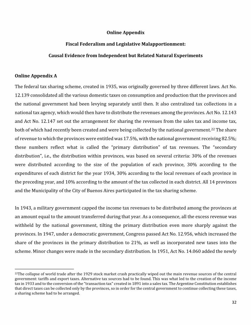
The federal tax sharing scheme, created in 1935, was originally governed by three different laws. Act No.

12.139 consolidated all the various domestic taxes on consumption and production that the provinces and

the national government had been levying separately until then. It also centralized tax collections in a

national tax agency, which would then have to distribute the revenues among the provinces. Act No. 12.143

and Act No. 12.147 set out the arrangement for sharing the revenues from the sales tax and income tax,

both of which had recently been created and were being collected by the national government.22 The share

of revenue to which the provinces were entitled was 17.5%, with the national government receiving 82.5%;

these numbers reflect what is called the “primary distribution” of tax revenues. The “secondary

distribution”, i.e., the distribution within provinces, was based on several criteria: 30% of the revenues

were distributed according to the size of the population of each province, 30% according to the

expenditures of each district for the year 1934, 30% according to the local revenues of each province in

the preceding year, and 10% according to the amount of the tax collected in each district. All 14 provinces

and the Municipality of the City of Buenos Aires participated in the tax sharing scheme.

In 1943, a military government capped the income tax revenues to be distributed among the provinces at

an amount equal to the amount transferred during that year. As a consequence, all the excess revenue was

withheld by the national government, tilting the primary distribution even more sharply against the

provinces. In 1947, under a democratic government, Congress passed Act No. 12.956, which increased the

share of the provinces in the primary distribution to 21%, as well as incorporated new taxes into the

scheme. Minor changes were made in the secondary distribution. In 1951, Act No. 14.060 added the newly

22The collapse of world trade after the 1929 stock market crash practically wiped out the main revenue sources of the central government: tariffs and export taxes. Alternative tax sources had to be found. This was what led to the creation of the income tax in 1933 and to the conversion of the “transaction tax” created in 1891 into a sales tax. The Argentine Constitution establishes that direct taxes can be collected only by the provinces, so in order for the central government to continue collecting these taxes, a sharing scheme had to be arranged.

32

created inheritance tax to the scheme, albeit with different distribution criteria: each district received

exactly the amount that had been collected within that district.

The 1950s brought changes in the federal organization of Argentina: new provinces were created out of

what had been known as the “national territories”, areas originally inhabited by indigenous populations

which were colonized in the late 19th century. The first new provinces were Chaco, in the northeast, and La

Pampa, in the center of the country, both created in 1951. Subsequently Misiones, also in the northeast,

was created in 1953 and Chubut, Formosa, Neuquén, Río Negro and Santa Cruz were created in 1955. All

these new provinces were gradually incorporated into the tax sharing scheme. Act No. 14.390 of 1954 –

which replaced Act No. 12.139- established a new criterion for the primary distribution of domestic tax

revenues which was based on the size of the populations of the provinces. Ultimately, when all the

remaining national territories, except Tierra del Fuego, were provincialized the following year, the share

of the provinces went up to 46% and that of the national government was reduced to 54%. In terms of the

secondary distribution, 98% of the revenues were distributed according to the population of each district;

this proportion fell to 84% in 1955, 82% in 1956 and 80% in 1957, while the proportions based on the

geographical location of the production of the taxed goods rose from 16% in 1955, to 18% in 1956 and to

20% in 1957. The remaining was distributed in inverse proportion to the size of the population.

With the advent of a new democratic government, Act No. 14.788 was passed in 1959, which gradually

increased the share of the provinces in the primary distribution to 40% (46% including the Municipality

of the City of Buenos Aires), up from 21%. The secondary distribution was as follows: 25% was distributed

according to the population, 25% according to the expenditures of each district, and 25% on the basis of

local revenues, while the other 25% was distributed equally among all the provinces. This regime remained

largely in place for more than a decade, although some changes were made in the primary distribution

during the military dictatorship of 1966-1973 that reduced the provinces’ share to 35%.

A major overhaul of the entire tax sharing scheme came in 1973 with the enactment of Act No. 20.221 by a

military government just days before the inauguration of a civilian government. This law created a single

scheme which covered all the taxes that had previously been administered separately. Under this new

scheme, the revenues from all the different taxes covered by the scheme were pooled into a single fund

that was then distributed, firstly, between the national government and the provinces and, secondly,

33

among the provinces. In terms of the primary distribution, the provinces and the national government each

received 48.5% of the revenues, while the remaining 3% was transferred to a regional development fund

created to finance infrastructure projects. The secondary distribution was based on three parameters:

population (65% of the revenues), development gap (25%) and population density (10%). The

development gap was defined as the average of the differences between indicators of housing quality, the

level of education and the number of motor vehicles relative to the size of the population in each district

and those of the Province of Buenos Aires and the City of Buenos Aires (taken together). This arrangement

clearly redistributed resources from the Buenos Aires region to the rest of the country. The population

density parameter (which measured the difference between each district’s population density and the

national average) was valid only for those districts whose density level was below the national average,

and six provinces (Buenos Aires, Córdoba, Entre Ríos, Misiones, Santa Fe and Tucumán) were therefore

excluded. Thus, scarcely populated provinces received a larger share than densely populated ones.

Act No. 20.221 was originally supposed to expire in 1980, but later in the same year that it was enacted

(1973), the democratically elected Congress voted to extend it to 1983. The scheme did not undergo any

major changes in the following years other than the inclusion of the value added tax, which was introduced

in 1975. However, in 1980, a military government decided to reform the system and reduced the share of

the provinces in the primary distribution to 32.6% (down from 48.5%) while, at the same time, it

incorporated social security contributions into the scheme. This led to changes in the secondary

distribution as well. The City of Buenos Aires was excluded from the sharing scheme in 1981 but was later

included again in 1983. Acts Nos. 22.923 and 22.924 incorporated these changes into the system, whose

expiry date was moved up to December 31st 1984.

In December 1983, a new democratic administration was elected. During 1984, the national government

and the provinces -now with elected governors- failed to reach an agreement on the design of a new tax

sharing scheme. On the first day of 1985, the scheme legally ceased to exist and the national government

had to resort to the use of national treasury contributions to transfer revenues to each province. Both the

primary and secondary distributions of tax revenues underwent significant changes. The Province of

Buenos Aires, for instance, received 17.1% of the share transferred to the provinces in 1985, while, in 1984,

the figure was 27.1%. A new law (Act No. 23.548) was not approved by the Congress until early 1988, and

the scheme that was enacted by that law was intended to be temporary. In fact, it was supposed to expire

34

at the end of 1989. In terms of the primary distribution, 43% of the revenues went to the national

government, while 57% went to the provinces.

The scheme created by Act No. 23.548 was automatically extended every year after 1989 and is still in

force. However, during the 1990s, several laws were passed that modified the scheme. There were also

sweeping changes in the relationship between the national government and the provinces, namely, the

complete decentralization of educational and health services together with a major reform in the social

security system. Thus, the parameters established in Act No. 23.548 provide no more than a very poor

indication of the actual shares received by each province in later years. During the 2000s, a further set of

regulations introduced more changes into the system. In December 2011, for instance, the revenues

covered by Act No. 23.548 represented 78% of the total transfers received by the provinces; the remaining

22% was transferred under the terms of another nine supplementary laws.

Online Appendix B

In this appendix we provide an overview of the sources of information on the relevant fiscal, political and

demographic variables that were used for this study.

For the fiscal variables, the sources were the annual reports of the Treasury Ministry (“Memorias del

Ministerio de Hacienda”) from 1935 to 1958, the statistical yearbooks of the General Tax Directorate

(“Boletines Estadísticos de la Dirección General Impositiva”) from 1958 to 1979, the annual reports of the

Treasury Department (“Memorias de la Secretaría de Hacienda”) from 1980 to 1984, and various

publications of the National Directorate for Provincial Fiscal Coordination (“Dirección Nacional de

Coordinación Fiscal con las Provincias”) from 1985 to 2011.

For every year, we computed the total amount of transfers received by each province under the terms of

the relevant legislation (see Table A.1) – that is, we excluded those transfers that corresponded to what are

known as “national treasury contributions” (aportes del tesoro nacional (ATN)), which are discretionary.

An exception was made for 1985-1987 when, because no tax sharing law was in force, all the revenues

were formally shared via national treasury contributions.

35

In the years between 1935 and 1940, the so-called “definitive” amounts of transfers were used. In that

period, the central government transferred a “provisional” amount of revenues during each year and, on

two occasions (1936 and 1942), later readjusted those amounts. These corrections were not significant in

most of the cases, however. In the 1990s, the amount of revenue transfers made under laws other than

Revenue Sharing Act No. 23.548 began to increase so significantly that, by the late 2000s, about 20% of the

tax revenue shared with the provinces were accounted for by those supplementary laws. We included all

these transfers in our computations since they are part of the overall tax sharing scheme.

36

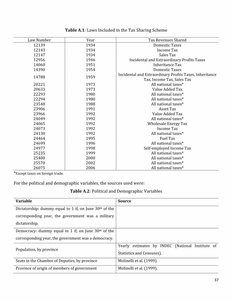
Table A.1: Laws Included in the Tax Sharing Scheme

Law Number Year Tax Revenues Shared 12139 1934 Domestic Taxes 12143 1934 Income Tax 12147 1934 Sales Tax 12956 1946 Incidental and Extraordinary Profits Taxes 14060 1951 Inheritance Tax 14390 1954 Domestic Taxes

14788 1959 Incidental and Extraordinary Profits Taxes, Inheritance Tax, Income Tax, Sales Tax

20221 1973 All national taxes* 20633 1973 Value Added Tax 22293 1980 All national taxes* 22294 1980 All national taxes* 23548 1988 All national taxes* 23906 1991 Asset Tax 23966 1992 Value Added Tax 24049 1992 All national taxes* 24065 1992 Wholesale Energy Tax 24073 1992 Income Tax 24130 1992 All national taxes* 24464 1995 Fuel Tax 24699 1996 All national taxes* 24977 1998 Self-employed Income Tax 25235 1999 All national taxes* 25400 2000 All national taxes* 25570 2002 All national taxes* 26075 2006 All national taxes*

*Except taxes on foreign trade.

For the political and demographic variables, the sources used were:

Table A.2: Political and Demographic Variables

Variable Source

Dictatorship: dummy equal to 1 if, on June 30th of the

corresponding year, the government was a military

dictatorship.

Democracy: dummy equal to 1 if, on June 30th of the

corresponding year, the government was a democracy.

Population, by province Yearly estimates by INDEC (National Institute of

Statistics and Censuses).

Seats in the Chamber of Deputies, by province Molinelli et al. (1999).

Province of origin of members of government Molinelli et al. (1999).

37

Online Appendix C

In this appendix we prove Proposition 1. We first prove two lemmas that characterize the solution of the

government’s problem under democracy and autocracy, respectively. Proposition 1 is a simple corollary of

these lemmas.

Lemma 1: Consider the public finance problem under democracy. Suppose that 𝐻𝐻2�𝑔𝑔, 𝜆𝜆𝑔𝑔𝑗𝑗� = 𝜆𝜆𝜃𝜃𝐻𝐻2�𝑔𝑔,𝑔𝑔𝑗𝑗�

for some 𝜃𝜃 and every 𝜆𝜆 > 0. Then, 𝑡𝑡1(𝐷𝐷) is given by:

𝑡𝑡1(𝐷𝐷) = �1 + �𝑁𝑁1𝜑𝜑1

1−𝑁𝑁1�

1𝜃𝜃�

−1

(14.)

Proof: Under democracy, the government’s problem is:

max(𝜏𝜏,𝑔𝑔,𝑔𝑔1,𝑔𝑔2)

�𝑊𝑊(𝐷𝐷) = 𝑡𝑡𝑃𝑃�𝜔𝜔1(𝐷𝐷)𝑝𝑝𝑃𝑃1 + �1 − 𝜔𝜔1(𝐷𝐷)�𝑝𝑝𝑃𝑃2��

where 𝜔𝜔1(𝐷𝐷) = 𝑁𝑁1𝜑𝜑1

𝑁𝑁1𝜑𝜑1+1−𝑁𝑁1 . The first-order conditions for welfare maximization are:

𝜕𝜕𝑊𝑊𝜕𝜕𝑔𝑔1

= 0 ⇒ 𝑁𝑁1𝜑𝜑1𝐻𝐻2�𝑔𝑔(𝐷𝐷),𝑔𝑔1(𝐷𝐷)� = ∆𝐷𝐷

𝜕𝜕𝑊𝑊𝜕𝜕𝑔𝑔2

= 0 ⇒ (1−𝑁𝑁1)𝐻𝐻2�𝑔𝑔(𝐷𝐷),𝑔𝑔2(𝐷𝐷)� = ∆𝐷𝐷

𝜕𝜕𝑊𝑊𝜕𝜕𝑔𝑔

= 0 ⇒ 𝑁𝑁1𝜑𝜑1𝐻𝐻1�𝑔𝑔(𝐷𝐷),𝑔𝑔1(𝐷𝐷)� + (1−𝑁𝑁1)𝐻𝐻1�𝑔𝑔(𝐷𝐷),𝑔𝑔2(𝐷𝐷)� = ∆𝐷𝐷

where ∆𝐷𝐷= �𝑁𝑁1𝜑𝜑1(1+𝛾𝛾)+(1−𝑁𝑁1)�𝑦𝑦𝑃𝑃2

𝑡𝑡𝑃𝑃(1+𝛾𝛾𝑁𝑁1)𝑦𝑦𝑃𝑃2+(1−𝑡𝑡𝑃𝑃)(1+𝛽𝛽𝑁𝑁1)𝑦𝑦𝑅𝑅

2. Since 𝐻𝐻 is strictly quasi-concave and satisfies the Inada conditions,

the first-order conditions are sufficient for a unique global maximum. After simple algebra we obtain:

𝑁𝑁1𝜑𝜑1𝐻𝐻2�𝑔𝑔(𝐷𝐷),𝑔𝑔1(𝐷𝐷)� = (1−𝑁𝑁1)𝐻𝐻2�𝑔𝑔(𝐷𝐷),𝑔𝑔2(𝐷𝐷)� =

= 𝑁𝑁1𝜑𝜑1𝐻𝐻1�𝑔𝑔(𝐷𝐷),𝑔𝑔1(𝐷𝐷)� + (1−𝑁𝑁1)𝐻𝐻1�𝑔𝑔(𝐷𝐷),𝑔𝑔2(𝐷𝐷)�

38

Since 𝐻𝐻2�𝑔𝑔, 𝜆𝜆𝑔𝑔𝑗𝑗� = 𝜆𝜆𝜃𝜃𝐻𝐻2�𝑔𝑔,𝑔𝑔𝑗𝑗�, from the first equality, we have:

𝑁𝑁1𝜑𝜑1�𝑔𝑔1(𝐷𝐷)�𝜃𝜃𝐻𝐻2(𝑔𝑔(𝐷𝐷), 1) = (1−𝑁𝑁1)�𝑔𝑔2(𝐷𝐷)�

𝜃𝜃𝐻𝐻2(𝑔𝑔(𝐷𝐷), 1)

Therefore, 𝑡𝑡1(𝐷𝐷) is given by:

𝑡𝑡1(𝐷𝐷) = �1 + �𝑁𝑁1𝜑𝜑1

1−𝑁𝑁1�

1𝜃𝜃�

−1

This completes the proof of Lemma 1. ∎

Lemma 2: Consider the public finance problem under an autocracy. Suppose that 𝐻𝐻2�𝑔𝑔, 𝜆𝜆𝑔𝑔𝑗𝑗� =

𝜆𝜆𝜃𝜃𝐻𝐻2�𝑔𝑔,𝑔𝑔𝑗𝑗� for some 𝜃𝜃 and every 𝜆𝜆 > 0. Then, 𝑡𝑡1(𝐷𝐷) depends only on (𝑁𝑁1,𝜑𝜑1), but 𝑡𝑡𝐹𝐹(𝐷𝐷) might depend on

�𝑦𝑦𝑃𝑃2,𝑦𝑦𝑅𝑅2,, 𝛾𝛾,𝛽𝛽� as well. Moreover, 𝑡𝑡1(𝐴𝐴) is given by:

𝑡𝑡1(𝐴𝐴) = �1 + �𝑁𝑁1

1 − 𝑁𝑁1�1𝜃𝜃�

−1

(15.)

Proof: Under autocracy, the government’s problem is:

max(𝜏𝜏,𝑔𝑔,𝑔𝑔1,𝑔𝑔2)

{𝑊𝑊(𝐴𝐴) = (1 − 𝑡𝑡𝑃𝑃)[𝑁𝑁1𝑝𝑝𝑅𝑅1 + 𝑁𝑁2𝑝𝑝𝑅𝑅2]}

The first-order conditions for this problem are: 𝜕𝜕𝑊𝑊𝜕𝜕𝑔𝑔1

= 0 ⇒ 𝑁𝑁1𝐻𝐻2�𝑔𝑔(𝐴𝐴),𝑔𝑔1(𝐴𝐴)� = ∆𝐴𝐴

𝜕𝜕𝑊𝑊𝜕𝜕𝑔𝑔2

= 0 ⇒ (1 − 𝑁𝑁1)𝐻𝐻2�𝑔𝑔(𝐴𝐴),𝑔𝑔2(𝐴𝐴)� = ∆𝐴𝐴

𝜕𝜕𝑊𝑊𝜕𝜕𝑔𝑔

= 0 ⇒ 𝑁𝑁1𝐻𝐻1�𝑔𝑔(𝐴𝐴),𝑔𝑔1(𝐴𝐴)� + (1 − 𝑁𝑁1)𝐻𝐻1�𝑔𝑔(𝐴𝐴),𝑔𝑔2(𝐴𝐴)� = ∆𝐴𝐴

39

where ∆𝐴𝐴= (1+𝛽𝛽𝑁𝑁1)𝑦𝑦𝑅𝑅2

𝑡𝑡𝑃𝑃(1+𝛾𝛾𝑁𝑁1)𝑦𝑦𝑃𝑃2+(1−𝑡𝑡𝑃𝑃)(1+𝛽𝛽𝑁𝑁1)𝑦𝑦𝑅𝑅

2. Therefore:

𝑁𝑁1𝐻𝐻2�𝑔𝑔(𝐴𝐴),𝑔𝑔1(𝐴𝐴)� = (1 − 𝑁𝑁1)𝐻𝐻2�𝑔𝑔(𝐴𝐴),𝑔𝑔2(𝐴𝐴)� = 𝑁𝑁1𝐻𝐻1�𝑔𝑔(𝐴𝐴),𝑔𝑔1(𝐴𝐴)� + (1 − 𝑁𝑁1)𝐻𝐻1�𝑔𝑔(𝐴𝐴),𝑔𝑔2(𝐴𝐴)�

Since 𝐻𝐻2�𝑔𝑔, 𝜆𝜆𝑔𝑔𝑗𝑗� = 𝜆𝜆𝜃𝜃𝐻𝐻2�𝑔𝑔,𝑔𝑔𝑗𝑗�, from the first equality, we have:

𝑁𝑁1�𝑔𝑔1(𝐴𝐴)�𝜃𝜃𝐻𝐻2(𝑔𝑔(𝐴𝐴), 1) = (1−𝑁𝑁1)�𝑔𝑔2(𝐴𝐴)�

𝜃𝜃𝐻𝐻2(𝑔𝑔(𝐴𝐴), 1)

Therefore, 𝑡𝑡1(𝐴𝐴) is given by:

𝑡𝑡1(𝐴𝐴) = �1 + �𝑁𝑁1

1 − 𝑁𝑁1�1𝜃𝜃�

−1

This completes the proof of Lemma 2. ∎

In order to prove Proposition 1, note that if 𝜑𝜑1 = 1, then expressions (14) and (15) are exactly the same,

while 𝑡𝑡1(𝐷𝐷) = �1 + � 𝜑𝜑1𝑁𝑁11−𝑁𝑁1

�1𝜃𝜃�−1

is increasing in 𝜑𝜑1. ∎

Example of Proposition 1: Assume �𝑔𝑔,𝑔𝑔𝑗𝑗� = 𝛼𝛼 (𝑔𝑔)1−𝜎𝜎

1−𝜎𝜎+ (1 − 𝛼𝛼) �𝑔𝑔

𝑗𝑗�1−𝜐𝜐

1−𝜐𝜐 , with 𝜎𝜎, 𝑝𝑝 ∈ (0,1). Note that

𝐻𝐻2�𝑔𝑔, 𝜆𝜆𝑔𝑔𝑗𝑗� = (1 − 𝛼𝛼)�𝜆𝜆𝑔𝑔𝑗𝑗�−𝜐𝜐

= (𝜆𝜆)−𝜐𝜐(1− 𝛼𝛼)�𝑔𝑔𝑗𝑗�−𝜐𝜐

= (𝜆𝜆)−𝜐𝜐𝐻𝐻2�𝑔𝑔,𝑔𝑔𝑗𝑗�. Hence, we can apply Proposition 1.

Under democracy, we have:

𝜕𝜕𝑊𝑊𝜕𝜕𝑔𝑔1

= 0 ⇒ 𝑁𝑁1𝜑𝜑1(1 − 𝛼𝛼)�𝑔𝑔1(𝐷𝐷)�−𝜐𝜐

= ∆𝐷𝐷

𝜕𝜕𝑊𝑊𝜕𝜕𝑔𝑔2

= 0 ⇒ (1−𝑁𝑁1)(1 − 𝛼𝛼)�𝑔𝑔2(𝐷𝐷)�−𝜐𝜐

= ∆𝐷𝐷

𝜕𝜕𝑊𝑊𝜕𝜕𝑔𝑔

= 0 ⇒ (𝑁𝑁1𝜑𝜑1 + 1−𝑁𝑁1)𝛼𝛼�𝑔𝑔(𝐷𝐷)�−𝜎𝜎

= ∆𝐷𝐷

40

where ∆𝐷𝐷= �𝑁𝑁1𝜑𝜑1(1+𝛾𝛾)+(1−𝑁𝑁1)�𝑦𝑦𝑃𝑃2

𝑡𝑡𝑃𝑃(1+𝛾𝛾𝑁𝑁1)𝑦𝑦𝑃𝑃2+(1−𝑡𝑡𝑃𝑃)(1+𝛽𝛽𝑁𝑁1)𝑦𝑦𝑅𝑅

2. Therefore, 𝑔𝑔1(𝐷𝐷) = �(1−𝛼𝛼)𝑁𝑁1𝜑𝜑1

∆𝐷𝐷�1𝜐𝜐, 𝑔𝑔2(𝐷𝐷) = �(1−𝛼𝛼)(1−𝑁𝑁1)

∆𝐷𝐷�1𝜐𝜐, and

𝑔𝑔(𝐷𝐷) = ��𝑁𝑁1𝜑𝜑1+1−𝑁𝑁1�𝛼𝛼∆𝐷𝐷

�1𝜎𝜎 and, hence:

𝑡𝑡1(𝐷𝐷) = �1 + �1−𝑁𝑁1𝑁𝑁1𝜑𝜑1

�1𝜐𝜐�−1

, 𝑡𝑡𝐹𝐹(𝐷𝐷)𝜏𝜏(𝐷𝐷)𝑦𝑦 = ��𝑁𝑁1𝜑𝜑1+1−𝑁𝑁1�𝛼𝛼∆𝐷𝐷

�1𝜎𝜎

𝜏𝜏(𝐷𝐷)𝑦𝑦 = ��𝑁𝑁1𝜑𝜑1+1−𝑁𝑁1�𝛼𝛼∆𝐷𝐷

�1𝜎𝜎 + �(1−𝛼𝛼)𝑁𝑁1𝜑𝜑1

∆𝐷𝐷�1𝜐𝜐 + �(1−𝛼𝛼)(1−𝑁𝑁1)

∆𝐷𝐷�1𝜐𝜐.

Under autocracy we have:

𝜕𝜕𝑊𝑊𝜕𝜕𝑔𝑔1

= 0 ⇒ 𝑁𝑁1(1 − 𝛼𝛼)�𝑔𝑔1(𝐷𝐷)�−𝜐𝜐

= ∆𝐴𝐴

𝜕𝜕𝑊𝑊𝜕𝜕𝑔𝑔2

= 0 ⇒ (1 − 𝑁𝑁1)(1 − 𝛼𝛼)�𝑔𝑔2(𝐷𝐷)�−𝜐𝜐

= ∆𝐴𝐴

𝜕𝜕𝑊𝑊𝜕𝜕𝑔𝑔

= 0 ⇒ 𝛼𝛼�𝑔𝑔(𝐷𝐷)�−𝜎𝜎

= ∆𝐴𝐴

where ∆𝐴𝐴= (1+𝛽𝛽𝑁𝑁1)𝑦𝑦𝑅𝑅2

𝑡𝑡𝑃𝑃(1+𝛾𝛾𝑁𝑁1)𝑦𝑦𝑃𝑃2+(1−𝑡𝑡𝑃𝑃)(1+𝛽𝛽𝑁𝑁1)𝑦𝑦𝑅𝑅

2. Therefore, 𝑔𝑔1(𝐴𝐴) = �(1−𝛼𝛼)𝑁𝑁1∆𝐴𝐴

�1𝜐𝜐, 𝑔𝑔2(𝐴𝐴) = �(1−𝛼𝛼)(1−𝑁𝑁1)

∆𝐴𝐴�1𝜐𝜐, and 𝑔𝑔(𝐴𝐴) =

� 𝛼𝛼∆𝐴𝐴�1𝜎𝜎 and, hence:

𝑡𝑡1(𝐴𝐴) = �1 + �1−𝑁𝑁1𝑁𝑁1

�1𝜐𝜐�−1

, 𝜏𝜏(𝐴𝐴)𝑦𝑦𝑡𝑡𝐹𝐹(𝐴𝐴) = � 𝛼𝛼∆𝐴𝐴�1𝜎𝜎

𝜏𝜏(𝐴𝐴)𝑦𝑦 = � 𝛼𝛼∆𝐴𝐴�1𝜎𝜎 + �(1−𝛼𝛼)𝑁𝑁1

∆𝐴𝐴�1𝜐𝜐 + �(1−𝛼𝛼)(1−𝑁𝑁1)

∆𝐴𝐴�1𝜐𝜐.

Suppose 1 < 𝜑𝜑1 < 1 + 𝛽𝛽. Then, 𝜑𝜑1

∆𝐷𝐷> 𝑁𝑁1𝜑𝜑1+1−𝑁𝑁1

∆𝐷𝐷> 1

∆𝐷𝐷> 1

∆𝐴𝐴. The proof of the first two inequalities is

immediate given that 𝜑𝜑1 > 1. The last inequality requires some extra work; in particular, we need to use

the assumption 𝛾𝛾 < 𝑦𝑦𝑅𝑅2−𝑦𝑦𝑃𝑃

2

𝑦𝑦𝑃𝑃2 . From 𝜑𝜑

1

∆𝐷𝐷> 𝑁𝑁1𝜑𝜑1+1−𝑁𝑁1

∆𝐷𝐷> 1

∆𝐷𝐷> 1

∆𝐴𝐴, we obtain:

41

𝑔𝑔1(𝐷𝐷) = �(1 − 𝛼𝛼)𝑁𝑁1𝜑𝜑1

∆𝐷𝐷�

1𝜐𝜐

> �(1 − 𝛼𝛼)𝑁𝑁1𝜑𝜑1

∆𝐷𝐷�

1𝜐𝜐

= 𝑔𝑔1(𝐴𝐴)

𝑔𝑔2(𝐷𝐷) = �(1 − 𝛼𝛼)(1 − 𝑁𝑁1)

∆𝐷𝐷�

1𝜐𝜐

> �(1 − 𝛼𝛼)(1− 𝑁𝑁1)

∆𝐴𝐴�

1𝜐𝜐

= 𝑔𝑔2(𝐴𝐴)

𝑔𝑔(𝐷𝐷) = �(𝑁𝑁1𝜑𝜑1 + 1−𝑁𝑁1)𝛼𝛼

∆𝐷𝐷�

1𝜎𝜎

> �𝛼𝛼∆𝐴𝐴�1𝜎𝜎

= 𝑔𝑔(𝐴𝐴)

𝜏𝜏(𝐷𝐷)𝑦𝑦 = 𝑔𝑔1(𝐷𝐷) + 𝑔𝑔2(𝐷𝐷) + 𝑔𝑔(𝐷𝐷) > 𝑔𝑔1(𝐴𝐴) + 𝑔𝑔2(𝐴𝐴) + 𝑔𝑔(𝐴𝐴) = 𝜏𝜏(𝐴𝐴)𝑦𝑦

Suppose that 1−𝑁𝑁11−𝑁𝑁1+𝛽𝛽𝑁𝑁1

< 𝜑𝜑1 < 1. Then, 1∆𝐷𝐷

> 𝑁𝑁1𝜑𝜑1+1−𝑁𝑁1∆𝐷𝐷

> 𝜑𝜑1

∆𝐷𝐷> 1

∆𝐴𝐴. The proof of the first two inequalities is

immediate given that 𝜑𝜑1 < 1. The last inequality requires some extra work; in particular, we need to use

the assumption 𝛾𝛾 < 𝑦𝑦𝑅𝑅2−𝑦𝑦𝑃𝑃

2

𝑦𝑦𝑃𝑃2 . From 1

∆𝐷𝐷> 𝑁𝑁1𝜑𝜑1+1−𝑁𝑁1

∆𝐷𝐷> 𝜑𝜑1

∆𝐷𝐷> 1

∆𝐴𝐴, we obtain:

𝑔𝑔1(𝐷𝐷) = �(1 − 𝛼𝛼)𝑁𝑁1𝜑𝜑1

∆𝐷𝐷�

1𝜐𝜐

> �(1 − 𝛼𝛼)𝑁𝑁1𝜑𝜑1

∆𝐷𝐷�

1𝜐𝜐

= 𝑔𝑔1(𝐴𝐴)

𝑔𝑔2(𝐷𝐷) = �(1 − 𝛼𝛼)(1 − 𝑁𝑁1)

∆𝐷𝐷�

1𝜐𝜐

> �(1 − 𝛼𝛼)(1− 𝑁𝑁1)

∆𝐴𝐴�

1𝜐𝜐

= 𝑔𝑔2(𝐴𝐴)

𝑔𝑔(𝐷𝐷) = �(𝑁𝑁1𝜑𝜑1 + 1−𝑁𝑁1)𝛼𝛼

∆𝐷𝐷�

1𝜎𝜎

> �𝛼𝛼∆𝐴𝐴�1𝜎𝜎

= 𝑔𝑔(𝐴𝐴)

𝜏𝜏(𝐷𝐷)𝑦𝑦 = 𝑔𝑔1(𝐷𝐷) + 𝑔𝑔2(𝐷𝐷) + 𝑔𝑔(𝐷𝐷) > 𝑔𝑔1(𝐴𝐴) + 𝑔𝑔2(𝐴𝐴) + 𝑔𝑔(𝐴𝐴) = 𝜏𝜏(𝐴𝐴)

Summing up, when 𝜑𝜑1 = 1, the shares of each jurisdiction under democracy and autocracy are the same,

but the share of the federal government, taxes and the level of public goods might differ. It is also immediate

that the share of district 1 is increasing in 𝜑𝜑1. As a consequence, we have: 𝑡𝑡1(𝐷𝐷)(𝜑𝜑1 < 1) <

𝑡𝑡1(𝐷𝐷)(𝜑𝜑1 = 1) = 𝑡𝑡1(𝐴𝐴) < 𝑡𝑡1(𝐷𝐷)(𝜑𝜑1 > 1). Finally, if 1−𝑁𝑁11−𝑁𝑁1+𝛽𝛽𝑁𝑁1

< 𝜑𝜑1 < 1 + 𝛽𝛽, then taxes and, hence, the

level of public goods, under democracy will be higher than under autocracy, i.e., 𝜏𝜏(𝐷𝐷) > 𝜏𝜏(𝐴𝐴).

This completes our example of Proposition 1. ∎

42