Fiscal Consolidation Policies and the Underground Economy:

The Case of Greece

Evi Pappa∗ Eugenia Vella†

December 9, 2014

Abstract

We revisit the effects of fiscal consolidation policies using a New Keynesian model withinvoluntary unemployment and an underground sector. We find that spending cuts inducea reallocation of production towards the formal sector, thus reducing tax evasion. On theother hand, tax hikes increase the incentives to produce in the less productive shadow sector,implying higher output and unemployment losses. We use the model to assess the recent fiscalconsolidation plans in Greece. Our results corroborate the evidence of increasing levels of taxevasion during these consolidations and point to significant output and welfare losses, whichcould be reduced substantially by combating the underground economy.

JEL classification: H3, E6Keywords: DSGE model, matching frictions, tax evasion, fiscal consolidation, policy

analysis.

∗Corresponding author, European University Institute, e-mail: evi.pappa@eui.eu†Jean Monnet Programme, European University Institute, e-mail: eugenia.vella@eui.eu

1

1 Introduction

The recent fiscal crisis has sparked a considerable amount of research measuring the macroeco-

nomic effects of fiscal consolidations.1 This literature, however, has left aside a crucial political

economy aspect, namely the presence of tax evasion. This is surprising, given that it is an im-

portant feature in many of the countries adopting consolidation policies, as Figure 1 shows. In

addition, there is growing evidence that tax evasion has increased in recent years. For example, a

recent report by the technical staff of the Spanish Finance Ministry (Gestha, 2014) indicates that

the shadow economy increased by 6.8 percentage points between 2008 and 2012, reaching 24.6%

of GDP. Using a model calibrated to firm-level data for Greece, Pappadà and Zylberberg (2014)

show that the increase in tax evasion can explain three quarters of the revenue leakages following

the 2010 VAT hikes, when only half of the expected increase in revenue was realized. Colombo et

al. (2014) also provide empirical evidence of a rise in the underground economy in recent years

by focusing on the role of the banking crisis. The aim of this paper is to revisit the effects of

government expenditure cuts and labor tax hikes on output, unemployment and welfare, when

tax evasion is present.

We treat tax evasion as synonymous with the shadow economy, which comprises “all market-

based, lawful production or trade of goods and services deliberately concealed from public authorities

in order to evade either payment of income, value added or other taxes, or social security con-

tributions” (Buehn and Schneider, 2012, p.175-176).2 Fiscal policy has an impact on the size of

the underground economy, since it affects the incentives to tax evade both directly, through the

tax burden, and indirectly, through its effects on the formal economy. Thus, a fiscal consolidation

can have important secondary effects if it generates a reallocation of resources between the formal

and informal sectors.

Many authors have studied whether it is preferable to rely on spending cuts or tax hikes when

consolidating deficit. Overall, the findings are not conclusive. Using multi-year fiscal consolidation

data for 17 OECD countries over the period 1980-2005, Alesina et al. (2013) show that expenditure-

based adjustments are typically associated with mild and short-lived recessions, and in some cases

with no recession at all, while tax-based corrections are followed by deep and prolonged recessions.

On the other hand, Erceg and Lindé (2013) reach a different conclusion. Using a two-country

Dynamic Stochastic General Equilibrium (DSGE) model of a currency union, they show that,

in the short run, a spending cut depresses output by more than a labor tax hike, because of the

limited accommodation by the central bank and the fixed exchange rate. However, this is reversed

in the long run as real interest and exchange rates adjust towards their flexible price levels.

We reassess the effects of fiscal consolidations in a model with price stickiness, search and

matching frictions, endogenous labor force participation, and tax evasion. The economy features

a regular and an informal sector, and the transactions in the latter sector are not recorded by the

government. Firms can hire informal labor to hide part of their production and evade payroll taxes.

1The implementation of the Maastricht Treaty in the mid 1990s initiated a wave of research on the effects ofconsolidations. For examples, see the survey in Perotti (1996).

2We use the terms "underground economy" and "shadow economy" interchangeably throughout the paper.

2

Households may also evade personal income taxation by reallocating their labor to the informal

sector. In each period, there is a positive probability that irregular employment is detected, in

which case the worker loses the job and the firm pays a fine. Following Erceg and Lindé (2013),

either labor tax rates or government consumption expenditures react to the deviation of the debt-

to-GDP ratio from a target value. Fiscal consolidation occurs when this target is hit by a negative

shock.

We calibrate the model for Greece. Our findings indicate that the presence of tax evasion

amplifies the negative effects of labor tax hikes on output and unemployment, while it mitigates

those of expenditure cuts. Tax evasion implies that a larger increase in the tax rate is needed to

reduce debt, and this amplifies the distortionary effects of the consolidation. Tax evasion further

increases the output losses after a tax hike because workers and firms reallocate resources to the

informal sector, increasing ineffi ciencies since this sector is less productive. On the other hand,

government spending cuts reduce tax evasion. The spending cut creates a positive wealth effect,

which increases consumption and investment and reduces labor force participation. This wealth

effect leads to an investment boom, and a subsequent rise in the capital stock, and agents reallocate

their labor search towards the formal sector, first, because it is more productive and, second,

because the formal labor market has a higher matching effi ciency and a lower job destruction rate.

Hence, the share of underground employment in total employment is reduced. Relative to standard

models, tax evasion increases the size of this wealth effect, thereby increasing the crowding-in of

private consumption, and reducing output losses. Labor tax hikes are costly in terms of welfare,

but spending cuts typically involve welfare gains, since private consumption increases and labor

supply decreases. The latter result is reversed, however, if government spending directly enters

the utility of households, or if agents are liquidity constrained.

We use our model to evaluate the impact of the recent consolidation policies in Greece. Despite

the fact that the consolidation plans rely heavily on spending cuts, the model predicts increasing

levels of tax evasion, as well as prolonged recessions and substantial welfare losses. There have

been considerable discussions in the policy arena about combating tax evasion. For example,

members of the European Parliament organized an event focusing on tax evasion in Ljubljana in

May 2013. The issue of reducing tax evasion also dominated the 2013 meeting of G8 leaders. To

quantitatively evaluate the welfare impact of fighting tax evasion, we perform a counterfactual

analysis of the consolidation plans when we increase the probability of tax audits. We find that

the battle is worth fighting as it significantly reduces the welfare losses from fiscal consolidation.

The remainder of the paper is organized as follows. In the next section we develop the model

and discuss the main theoretical results. Section 3 presents the policy evaluation exercise and

Section 4 concludes.

2 The Model

We construct a DSGE model featuring search and matching frictions, endogenous labor decisions,

and sticky prices in the short run. There are two types of firms in the economy: (i) competitive

firms that produce intermediate goods in either the formal or informal sector, and (ii) monopolistic

3

Figure 1: Shadow Economy Estimates in European Countries

Shadow Economy (% GDP), Average over 1999-2010Source: Schneider and Buehn (2012).

Note: The dotted line indicates the average for the countries considered.

retailers that use all intermediate varieties to produce differentiated retail goods, which are then

costlessly aggregated into a final consumption good. Price rigidities arise at the retail level,

while labor market frictions occur in the production of intermediate goods. Intermediate firms

can choose to produce in the informal sector in order to evade the payroll taxes paid on formal

employment. In each period, they face a probability of being inspected by the fiscal authorities

and convicted of tax evasion, in which case they pay a penalty, and the employment match is

terminated. There is a representative household consisting of formal and informal employees,

unemployed jobseekers and labor force non-participants. Jobseekers can choose to search in the

informal sector in order to evade income taxes. The household rents out its private capital to the

intermediate firms, and purchases the final consumption good. The government collects taxes from

the regular sector and uses them to finance public expenditures and the provision of unemployment

benefits.

2.1 Labor markets

We account for the imperfections and transaction costs in the labor market by assuming that jobs

are created through a matching function. For j = F, I denoting the formal and informal sectors,

let υjt be the number of vacancies and ujt the number of jobseekers in each sector. We assume

matching functions of the form:

mjt = µj1(υjt )

µ2(ujt )1−µ2 (1)

4

where we allow for differences in the effi ciency of the matching process, µj1, in the two sectors. In

each sector we can define the probability of a jobseeker being hired, ψhjt , and of a vacancy being

filled, ψfjt , as follows:

ψhjt ≡mjt

ujt, ψfjt ≡

mjt

υjt

In each period, jobs in the formal sector are destroyed at a constant fraction, σF , and mFt new

matches are formed. The law of motion of formal employment, nFt , is thus given by:

nFt+1 = (1− σF )nFt +mFt (2)

In the informal sector there is an exogenous fraction of jobs destroyed in each period, σI , as well

as a probability, ρ, that an informal employee loses their job due to an audit. The law of motion

of informal employment, nIt , is given by:

nIt+1 = (1− ρ− σI)nIt +mIt (3)

2.2 Households

The representative household consists of a continuum of infinitely lived agents. The members of

the household derive utility from leisure, which corresponds to the fraction of members that are

out of the labor force, lt, and a consumption bundle, cct, defined as:

cct = [α1(ct)α2 + (1− α1)(gt)

α2 ]1α2

where gt denotes public consumption, taken as exogenous by the household, and ct is private

consumption. The elasticity of substitution between the private and public goods is given by1

1−α2.3 The instantaneous utility function is given by:

U(cct, lt) =cc1−ηt

1− η + Φl1−ϕt

1− ϕ

where η is the inverse of the intertemporal elasticity of substitution, Φ > 0 is the relative preference

for leisure, and ϕ is the inverse of the Frisch elasticity of labor supply.

At any point in time, a fraction nFt (nIt ) of the household members are formal (informal)

employees. Campolmi and Gnocchi (2014), Brückner and Pappa (2012) and Bermperoglou et

al. (2014) have added a labor force participation choice in New Keynesian models of equilibrium

unemployment. Following Ravn (2008), the participation choice is modelled as a trade-offbetween

the cost of giving up leisure and the prospect of finding a job. In particular, the household chooses

the fraction of the unemployed actively searching for a job, ut, and the fraction which are out of

3When α2 approaches one, ct and gt are perfect substitutes. They are instead perfect complements if α2 tendsto minus infinity. α2 = 0 nests the Cobb-Douglas specification.

5

the labor force and enjoying leisure, lt, so that:

nFt + nIt + ut + lt = 1 (4)

The household chooses the fraction of jobseekers searching in each sector: a share st of jobseekers

look for a job in the informal sector, while the remainder, (1− st), seek employment in the formalsector. That is, uIt ≡ stut and uFt ≡ (1− st)ut.

The household owns the capital stock, which evolves over time according to:

kt+1 = it + (1− δ)kt −ω

2

(kt+1

kt− 1

)2

kt (5)

where it is investment, δ is a constant depreciation rate and ω2

(kt+1

kt− 1)2kt are adjustment costs.

The intertemporal budget constraint is given by:

(1 + τ ct)ct + it +Bt+1πt+1

Rt≤ rtkt + (1− τnt )wFt n

Ft + wIt n

It +$uFt +Bt + Πp

t − Tt (6)

where πt ≡ pt/pt−1 is the gross inflation rate, wjt , j = F, I, are the real wages in the two sectors, rt

is the real return on capital, $ denotes unemployment benefits, available only to formal jobseekers

(see e.g. Boeri and Garibaldi, 2007), Bt is the real government bond holdings, Rt is the gross

nominal interest rate, Πpt are the profits of the monopolistic retailers, discussed below, and τ

ct , τ

nt

and Tt represent taxes on private consumption, labor income and lump-sum taxes respectively.

The household maximizes expected lifetime utility subject to (1) for each j, (2), (3), (4), (5),

and (6). Taking as given njt , they choose ut, st (which together determine lt) and njt+1, as well as

ct, kt+1 and Bt+1.

It is convenient to define the marginal value to the household of having an additional member

employed in each sector, as follows:

V hnF t = λctw

Ft (1− τnt )− Φl−ϕt + (1− σF )λnF t (7)

V hnI t = λctw

It − Φl−ϕt + (1− ρ− σI)λnI t (8)

where λnF t, λnI t and λct are the multipliers in front of (2), (3) and (6) respectively.

2.3 Production

2.3.1 Intermediate goods firms

Intermediate goods are produced with two different technologies:

xFt = (AFt nFt )1−αF (kt)

αF (9)

xIt = (AItnIt )

1−αI (10)

6

where Ajt denotes total factor productivity in sector j. Following the literature, we assume that

the informal production technology uses labor inputs only (see e.g. Busato and Chiarini, 2004).

Firms maximize the discounted value of future profits, subject to (2) and (3). That is, they

take the number of workers currently employed in each sector, njt , as given and choose the number

of vacancies posted in each sector, υjt , so as to employ the desired number of workers next period,

njt+1. Here, firms adjust employment by varying the number of workers (extensive margin) rather

than the number of hours per worker (intensive margin). According to Hansen (1985), most of

the employment fluctuations arise from movements in this margin. Firms also decide the amount

of private capital, kt, needed for production. They face a probability, ρ, of being inspected by

the fiscal authorities, convicted of tax evasion and forced to pay a penalty, which is a fraction,

γ, of their total revenues. We assume that, once they are produced, there is no differentiation

between intermediate goods from the different sectors. In other words, we assume that formal and

informal goods are perfect substitutes, so that they are sold at the same price, pxt (see e.g. Orsi

et al., 2014). Hence the problem of an intermediate firm is summarized by the following Bellman

equation:

Q(nFt , nIt ) = max

kt,υFt ,υIt

{(1− ργ) pxt (xFt + xIt )− (1 + τ st )w

Ft n

Ft − wIt nIt − rtkt

− κFυFt − κIυIt + Et[Λt,t+1Q(nFt+1, n

It+1)

] }where τ st is a payroll tax, κ

j is the cost of posting a new vacancy in sector j, and Λt,t+1 ≡βUcc,t+1

Ucc,t= β

(cct+1

cct

)−ηis a discount factor. The first-order conditions are:

rt = (1− ργ) pxt

(αFxFtkt

)(11)

κF

ψfFt= EtΛt,t+1

[(1− ργ) pxt+1(1− αF )

xFt+1

nFt+1

− (1 + τ st+1)wFt+1 +(1− σF )κF

ψfFt+1

](12)

κI

ψfIt= EtΛt,t+1

[(1− ργ) pxt+1(1− αI)

xIt+1

nIt+1

− wIt+1 +(1− ρ− σI)κI

ψfIt+1

](13)

According to (11)-(13), the net value of the marginal product of private capital should equal the

real rental rate and the expected marginal cost of hiring a worker in each sector j should equal

the expected marginal benefit. The latter includes the net value of the marginal product of labor

minus the wage, augmented by the payroll tax in the formal sector, plus the continuation value.

For convenience, we define the value of the marginal formal and informal job for the interme-

diate firm:

V fnF t

= (1− ργ) pxt (1− αF )xFtnFt− (1 + τ st )w

Ft +

(1− σF )κF

ψfFt(14)

V fnI t

= (1− ργ) pxt (1− αI)xIt

nIt− wIt +

(1− ρ− σI)κI

ψfIt(15)

7

2.3.2 Retailers

There is a continuum of monopolistically competitive retailers indexed by i on the unit interval.

Retailers buy intermediate goods and differentiate them with a technology that transforms one

unit of intermediate goods into one unit of retail goods, and thus the relative price of intermediate

goods, pxt , coincides with the real marginal cost faced by the retailers. Let yit be the quantity of

output sold by retailer i. The final consumption good can be expressed as:

yt =

[∫ 1

0(yit)

ε−1ε di

] εε−1

(16)

where ε > 1 is the constant elasticity of demand for retail goods. The final good is sold at a price

pt =[∫ 1

0 p1−εit di

] 11−ε. The demand for each intermediate good depends on its relative price and on

aggregate demand:

yit =

(pitpt

)−εyt (17)

Following Calvo (1983), we assume that in any given period each retailer can reset its price with

a fixed probability (1− χ). Hence, the price index is given by:

pt =[(1− χ)(p∗t )

1−ε + χ(pt−1)1−ε] 11−ε (18)

Firms that are able to reset their price choose p∗it so as to maximize expected profits given by:

Et

∞∑s=0

χsΛt,t+s(p∗it − pxt+s)yit+s

The resulting expression for p∗it is:

p∗it =ε

ε− 1

Et∑∞

s=0 χsΛt,t+sp

xt+syit+s

Et∑∞

s=0 χsΛt,t+syit+s

(19)

2.4 Government

Government expenditure consists of consumption purchases and unemployment benefits, while

revenues come from the collected fines and the payroll, consumption, and labor income taxes, as

well as the lump-sum taxes. The government deficit is therefore defined by:

DFt = gt +$uFt − TRt − ργpxt (xFt + xIt ) (20)

where TRt ≡ (τnt + τ st )wFt n

Ft + τ ctct + Tt denotes tax revenues.

The government budget constraint is given by:

Bt +DFt = R−1t Bt+1πt+1 (21)

8

We assume that Tt, τ st , and τct are constant and fixed at their steady state levels, and we do not

consider them as active instruments for fiscal consolidation. In our model, the effects of payroll

taxes are very similar to labor income taxes. Consumption taxes can have different effects, but

they generally constitute a relatively small source of tax revenues. Thus, in line with Erceg and

Lindé (2013), the government has two potential fiscal instruments, g and τn. We consider each

instrument separately, assuming that if one is active, the other remains fixed at its steady state

value. For Ψ ∈ {g, τn}, we assume fiscal rules of the form:

Ψt = Ψ(1−βΨ0) ΨβΨ0t−1 exp{(1− βΨ0)[βΨ1(bt − b∗t ) + βΨ2(∆bt+1 −∆b∗t+1)]} (22)

where bt = Btytis the debt-to-GDP ratio, and b∗t is the target value for this ratio, given by the

AR(2) process:

log b∗t+1 − log b∗t = µb + ρ1(log b∗t − log b∗t−1)− ρ2 log b∗t − εbt (23)

where εbt is a white noise shock representing a fiscal consolidation.

2.5 Closing the model

Monetary Policy There is an independent monetary authority that sets the nominal interest

rate as a function of current inflation according to the rule:

Rt = R exp{ζπ(πt − 1)} (24)

where R is the steady state value of the nominal interest rate.

Goods Markets Total output must equal private and public demand. The aggregate resource

constraint is thus given by:

yt = ct + it + gt + κFυFt + κIυIt (25)

The aggregate price index, pt, is given by (18) and (19). The return on private capital, rt, adjusts

so that the capital demanded by the intermediate goods firm, given by (11), is equal to the stock

held by the household.

Bargaining over wages Wages in both sectors are determined by ex-post (after matching)

Nash bargaining. Workers and firms split rents and the part of the surplus they receive depends

on their bargaining power. We denote by ϑj ∈ (0, 1) the firms’bargaining power in sector j. The

Nash bargaining problem is to maximize the weighted sum of log surpluses:

maxwjt

{(1− ϑj) log V h

njt + ϑj log V fnjt

}

9

where V hnjt

and V fnjt

are defined in equations (7), (8), (14) and (15). As shown in the Appendix,

wages are given by:

wFt =(1− ϑF )

(1 + τ st )

((1− ργ) pxt (1− αF )

xFtnFt

+(1− σF )κF

ψfFt

)+

ϑF

λct(1− τnt )

(Φl−ϕt −(1−σF )λnF t

)(26)

wIt = (1−ϑI)(

(1− ργ) pxt (1− αI)xIt

nIt+

(1− ρ− σI)κI

ψfIt

)+ϑI

λct

(Φl−ϕt − (1−ρ−σI)λnI t

)(27)

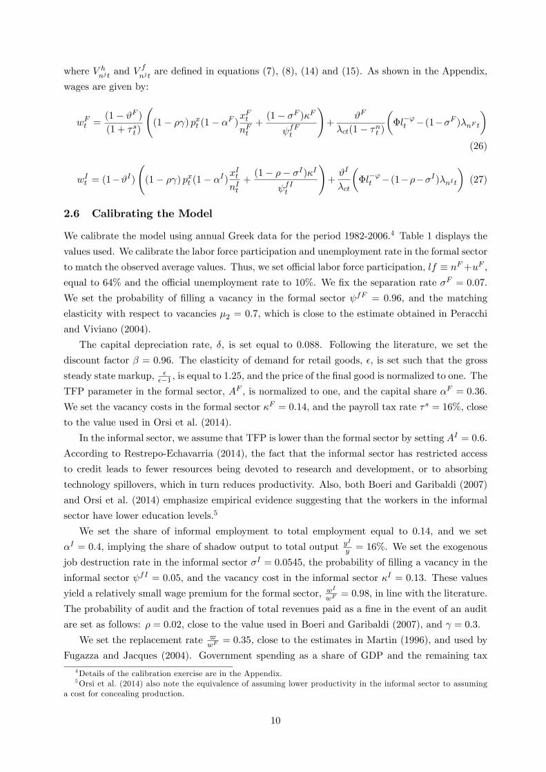
2.6 Calibrating the Model

We calibrate the model using annual Greek data for the period 1982-2006.4 Table 1 displays the

values used. We calibrate the labor force participation and unemployment rate in the formal sector

to match the observed average values. Thus, we set offi cial labor force participation, lf ≡ nF +uF ,

equal to 64% and the offi cial unemployment rate to 10%. We fix the separation rate σF = 0.07.

We set the probability of filling a vacancy in the formal sector ψfF = 0.96, and the matching

elasticity with respect to vacancies µ2 = 0.7, which is close to the estimate obtained in Peracchi

and Viviano (2004).

The capital depreciation rate, δ, is set equal to 0.088. Following the literature, we set the

discount factor β = 0.96. The elasticity of demand for retail goods, ε, is set such that the gross

steady state markup, εε−1 , is equal to 1.25, and the price of the final good is normalized to one. The

TFP parameter in the formal sector, AF , is normalized to one, and the capital share αF = 0.36.

We set the vacancy costs in the formal sector κF = 0.14, and the payroll tax rate τ s = 16%, close

to the value used in Orsi et al. (2014).

In the informal sector, we assume that TFP is lower than the formal sector by setting AI = 0.6.

According to Restrepo-Echavarria (2014), the fact that the informal sector has restricted access

to credit leads to fewer resources being devoted to research and development, or to absorbing

technology spillovers, which in turn reduces productivity. Also, both Boeri and Garibaldi (2007)

and Orsi et al. (2014) emphasize empirical evidence suggesting that the workers in the informal

sector have lower education levels.5

We set the share of informal employment to total employment equal to 0.14, and we set

αI = 0.4, implying the share of shadow output to total output yI

y = 16%. We set the exogenous

job destruction rate in the informal sector σI = 0.0545, the probability of filling a vacancy in the

informal sector ψfI = 0.05, and the vacancy cost in the informal sector κI = 0.13. These values

yield a relatively small wage premium for the formal sector, wI

wF= 0.98, in line with the literature.

The probability of audit and the fraction of total revenues paid as a fine in the event of an audit

are set as follows: ρ = 0.02, close to the value used in Boeri and Garibaldi (2007), and γ = 0.3.

We set the replacement rate $wF

= 0.35, close to the estimates in Martin (1996), and used by

Fugazza and Jacques (2004). Government spending as a share of GDP and the remaining tax4Details of the calibration exercise are in the Appendix.5Orsi et al. (2014) also note the equivalence of assuming lower productivity in the informal sector to assuming

a cost for concealing production.

10

Table 1: Calibration Values

Parameter Description Full Modelβ Discount Factor 0.96δ Depreciation Rate 0.088α1 Share of Private Consumption in Utility 1η Inverse Elasticity of Intertemporal Substitution 2ϕ Inverse Frisch Elasticity of Labor Supply 2Φ Relative Utility from Leisure 0.7lf Offi cial Labor Force Participation 0.64uF

lf Offi cial Unemployment Rate 0.1u

1−l Actual Unemployment Rate 0.09s Share of Informal Jobseekers to Total 0.10nI

n Share of Informal Employment to Total 0.14σF Exogenous Job Destruction Rate - Formal Sector 0.07σI Exogenous Job Destruction Rate - Informal Sector 0.0545ρ Auditing Probability 0.02µF1 Matching Effi ciency - Formal Sector 0.85µI1 Matching Effi ciency - Informal Sector 0.12µ2 Elasticity of Matching to Vacancies 0.7ψfF Probability of Filling a Vacancy - Formal Sector 0.96ψfI Probability of Filling a Vacancy - Informal Sector 0.05ψhF Probability of Finding a Job - Formal Sector 0.63ψhI Probability of Finding a Job - Informal Sector 0.91AF TFP - Formal Sector 1AI TFP - Informal Sector 0.6αF Capital Share - Formal Sector 0.36αI Production Function Parameter - Informal Sector 0.4yI

y Share of Underground Output in Total 0.16κF Vacancy Costs - Formal Sector 0.14κF

wFVacancy Costs/Wage 0.21

κI Vacancy Costs - Informal Sector 0.13ε Price Elasticity of Demand 5ϑF Firm’s Bargaining Power - Formal Sector 0.22ϑI Firm’s Bargaining Power - Informal Sector 0.80wI

wFFormal/Informal Wage Differentials 0.98

gy Government Expenditure-to-GDP Ratio 0.05$wF

Replacement Rate 0.35τn Labor Income Tax Rate 0.4τ s Payroll Tax Rate 0.16τ c Consumption Tax Rate 0.18γ Proportional Fine in Case of Auditing 0.3DFy Deficit-to-GDP Ratio -0.04b Debt-to-GDP Ratio 1.45

ρ1, ρ2 Debt-to-GDP Target Parameters 0.85, 0.0001χ Price Stickiness 0.25ω Capital Adjustment Costs 0.5ζπ Taylor Rule Parameter 1.5

11

rates are set as follows: gy = 5%, τn = 40%, in line with Orsi et al. (2014), and τ c = 18%. The

steady state debt-to-GDP ratio b = 145%.

We begin by assuming purely wasteful government expenditure, setting α1 = 1, and will

consider utility enhancing government spending as an extension. Regarding the inverse elasticity

of intertemporal substitution, η, much of the literature cites the econometric estimates of Hansen

and Singleton (1983), which place it “between 0 and 2”, and often choose a value greater than

unity. In our calibration, we set η = 2 and we perform sensitivity analysis by considering η equal

to 0.5 and 1. The inverse of the Frisch elasticity, ϕ, is set equal to 2. Finally, we set the inflation

targeting parameter in the Taylor rule ζπ = 1.5, the capital adjustment costs ω = 0.5 and the

price-stickiness parameter χ = 0.25.

2.7 Results

We present responses following a negative debt-target shock (see Erceg and Lindé, 2013). We

compare the effects of a 5% reduction in the desired long run debt target, which is achieved after

10 years, either through a fall in government consumption expenditure, or a hike in labor tax

rates.6

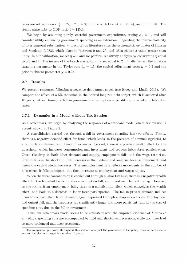
2.7.1 Dynamics in a Model without Tax Evasion

As a benchmark, we begin by analyzing the responses of a standard model where tax evasion is

absent, shown in Figure 2.

A consolidation carried out through a fall in government spending has two effects. Firstly,

there is a negative demand effect for firms, which leads, in the presence of nominal rigidities, to

a fall in labor demand and hence in vacancies. Second, there is a positive wealth effect for the

household, which increases consumption and investment and reduces labor force participation.

Given the drop in both labor demand and supply, employment falls and the wage rate rises.

Output falls in the short run, but increases in the medium and long run because investment, and

hence the capital stock, increases. The unemployment rate reflects movements in the number of

jobseekers: it falls on impact, but then increases as employment and wages adjust.

When the fiscal consolidation is carried out through a labor tax hike, there is a negative wealth

effect for the household which makes consumption fall, and investment fall with a lag. However,

as the return from employment falls, there is a substitution effect which outweighs the wealth

effect, and leads to a decrease in labor force participation. The fall in private demand induces

firms to contract their labor demand, again expressed through a drop in vacancies. Employment

and output fall, and the responses are significantly larger and more persistent than in the case of

spending cuts, due to the fall in investment.

Thus, our benchmark model seems to be consistent with the empirical evidence of Alesina et

al. (2013); spending cuts are accompanied by mild and short-lived recessions, while tax hikes lead

to more prolonged and deep recessions.

6For comparison purposes, throughout this section we adjust the parameters of the policy rules for each case toensure that the debt target is met after 10 years.

12

Figure2:ImpulseResponseFunctionsoftheBenchmarkModel(withoutTaxEvasion)

24

68

10

­1.5­1

­0.5

0

PAR

TIC

IPA

TIO

N R

ATE

24

68

10

­0.4

­0.2

0

0.2

PRIV

ATE

 CO

NSU

MPT

ION

24

68

10

­2­1012

INVE

STM

ENT

24

68

10

­0.05

0

0.05

GR

OSS

 REA

L IN

TER

EST 

RA

TE

24

68

10

­0.5

0

0.5

CA

PITA

L

24

68

10

­5­4­3­2­1012

VAC

AN

CIE

S

24

68

10

­2­101234JO

BSE

EKER

S

24

68

10­1

.2­1

­0.8

­0.6

­0.4

­0.2

0EM

PLO

YMEN

T

24

68

10

0

0.1

0.2

0.3

0.4

WA

GE

24

68

10

­0.8

­0.6

­0.4

­0.2

0

0.2

OU

TPU

T

24

68

10

­15

­10­505

AC

TIVE

 INST

RU

MEN

T

24

68

10

12345678TA

X R

EVEN

UE

24

68

10

­16

­14

­12

­10­8­6­4­2

DEF

ICIT

­TO

­GD

P R

ATI

O

24

68

10

­5­4­3­2­10D

EBT­

TO­G

DP 

RA

TIO

24

68

10

­2­101234

UN

EMPL

OYM

ENT 

RA

TE

SPEN

DIN

G C

UT

LAB

OR

 TA

X H

IKE

13

2.7.2 Dynamics in a Model with Tax Evasion

We now move to the full model with tax evasion. Figure 3 presents the responses of the formal

sector and of fiscal variables, and Figure 4 shows the responses in the informal sector.

To start with, notice that the response of the formal sector is qualitatively similar to the

benchmark model. However, there is an additional channel at play. For the case of tax hikes,

unemployed jobseekers reallocate their labor supply and the intermediate firms reallocate their

labor demand towards the informal sector. Tax hikes provide direct incentives for jobseekers to

search in the informal sector because of the higher tax rates in the formal sector. At the same time,

intermediate firms find it profitable to post vacancies in the informal sector because of the fall in

the informal wage. The fall in investment, and hence the capital stock, lowers the productivity

differential between the two sectors, and further provides incentives for agents to reallocate to the

informal sector. As a result, shadow employment as a share of total employment increases.

For the case of expenditure cuts, the negative demand effect of the spending cut affects both

formal and informal production, leading to a reduction in labor demand in both sectors. Similarly,

as labor force participation falls, there is a reduction in unemployed jobseekers in both sectors.

This causes a contraction in total employment. Moreover, there is a reallocation of labor towards

the formal sector; underground employment as a share of total employment falls. This happens

for two reasons. Firstly, the formal labor market has a higher matching effi ciency, and a lower

job destruction rate. Secondly, in addition to having a higher TFP level, the rise in the capital

stock further increases the productivity of the formal sector relative to the informal sector. In

order to take advantage of these effi ciency gains, and thus mitigate the negative effects of the

fiscal contraction, agents optimally choose to reallocate towards the formal sector.

2.7.3 A More Detailed Comparison

Figure 5 compares the responses of output, the unemployment rate and welfare in the two models.7

For spending cuts, shown in the top panel, the presence of tax evasion generates smaller losses

in output, a drop in the unemployment rate at all horizons, and larger welfare gains. With tax

evasion, the tax adjustments required to achieve a given change in deficit are larger, and thus,

following a spending cut, taxes in the future are expected to fall by more. In other words, there

is an amplification of the positive wealth effect. Hence the rise in consumption and the fall in

labor force participation are larger relative to the model without tax evasion, making welfare gains

larger. The increased crowding-in of private consumption mitigates the negative demand effect

for the firms, thereby mitigating output losses. The larger reduction in labor force participation

implies a fall in the number of formal jobseekers, and hence in the offi cial unemployment rate, at

all horizons.

For tax hikes, shown in the middle panel, the presence of tax evasion amplifies the output

losses, particularly in the long run. This is due to the loss of tax revenue from tax evasion,

implying that larger increases in tax rates are needed to reduce debt-to-GDP. This increases the

distortionary effects of the consolidation, leading to a larger drop in labor force participation,

7Welfare is computed as per-period steady state consumption equivalents.

14

Figure3:ImpulseResponseFunctionsoftheFullModel(withTaxEvasion)

24

68

10

­1.5­1

­0.5

0

PAR

TIC

IPA

TIO

N R

ATE

24

68

10

­1.5­1

­0.5

0

CO

NSU

MPT

ION

24

68

10

­10­50

INVE

STM

ENT

24

68

10­0

.4

­0.3

­0.2

­0.1

0

0.1

0.2

GR

OSS

 REA

L IN

TER

EST 

RA

TE

24

68

10­5­4­3­2­101

CA

PITA

L

24

68

10

­40

­30

­20

­10010

FOR

MA

L VA

CA

NC

IES

24

68

10

­40

­30

­20

­10010

FOR

MA

L JO

BSE

EKER

S

24

68

10­7­6­5­4­3­2­10

FOR

MA

L EM

PLO

YMEN

T

24

68

10

­1

­0.5

0

0.51

1.5

FOR

MA

L W

AG

E

24

68

10

­5­4­3­2­10

FOR

MA

L O

UTP

UT

24

68

10

­15

­10­5051015

AC

TIVE

 INST

RU

MEN

T

24

68

10

123456

TAX 

REV

ENU

E

24

68

10

­16

­14

­12

­10­8­6­4­2

DEF

ICIT

­TO

­GD

P R

ATI

O

24

68

10

­5­4­3­2­10

DEB

T­TO

­GD

P R

ATI

O

24

68

10

­40

­30

­20

­1001020O

FFIC

IAL 

UN

EMPL

OYM

ENT 

RA

TE

SPEN

DIN

G C

UT

LAB

OR

 TA

X H

IKE

15

Figure4:ImpulseResponseFunctionsoftheFullModel-UndergroundSector

12

34

56

78

91

01

1­2

0

­10010

20

30

40

50

UN

DE

RG

RO

UN

D V

AC

AN

CIE

S

12

34

56

78

91

01

1

­10010

20

30

40

50

60

UN

DE

RG

RO

UN

D J

OB

SE

EK

ER

S

12

34

56

78

91

01

1

­6­5­4­3­2­10

UN

DE

RG

RO

UN

D W

AG

E

12

34

56

78

91

01

10510

15

UN

DE

RG

RO

UN

D E

MP

LO

YM

EN

T

12

34

56

78

91

01

102468

UN

DE

RG

RO

UN

D O

UT

PU

T

SP

EN

DIN

G C

UT

LA

BO

R T

AX

 HIK

E

16

Figure 5: Comparison of Benchmark and Full Model

1 2 3 4 5 6 7 8 9 1 0 1 1

­0 .1 5

­0 .1

­0 .0 5

0

0 .0 5

0 .1

0 .1 5

0 .2

0 .2 5

0 .3

0 .3 5

FIN A L O U TP U T

1 2 3 4 5 6 7 8 9 1 0 1 1

­2

­1 .5

­1

­0 .5

0

0 .5

O FFIC IA L U N E M P LO Y M E N T R A TE

1 2 3 4 5 6 7 8 9 1 0 1 1

0 .2

0 .4

0 .6

0 .8

1

1 .2

W E LFA R E

B E N C H M A R K  M O D E L

FU LL M O D E L

Government Expenditure Cuts

1 2 3 4 5 6 7 8 9 1 0 1 1

­3

­2 .5

­2

­1 .5

­1

­0 .5

FIN A L O U TP U T

1 2 3 4 5 6 7 8 9 1 0 1 1

­4 0

­3 0

­2 0

­1 0

0

1 0

2 0

O FFIC IA L U N E M P LO Y M E N T R A TE

1 2 3 4 5 6 7 8 9 1 0 1 1

­0 .6

­0 .5 5

­0 .5

­0 .4 5

­0 .4

­0 .3 5

­0 .3

­0 .2 5

­0 .2

­0 .1 5

­0 .1

W E LFA R E

B E N C H M A R K  M O D E L

FU LL M O D E L

Labor Tax Hikes

1 2 3 4 5 6 7 8 9 1 0 1 1

­2

­1 . 5

­1

­0 . 5

0

0 . 5

FIN A L O U TP U T

1 2 3 4 5 6 7 8 9 1 0 1 1­2

­1 . 5

­1

­0 . 5

0

O FFIC IA L U N E M P LO Y M E N T R A TE

1 2 3 4 5 6 7 8 9 1 0 1 1

­0 . 0 5

0

0 . 0 5

0 . 1

0 . 1 5

0 . 2

W E LFA R E

B E N C H M A R K  M O D E L

FU LL M O D E L

Mixed Consolidation

17

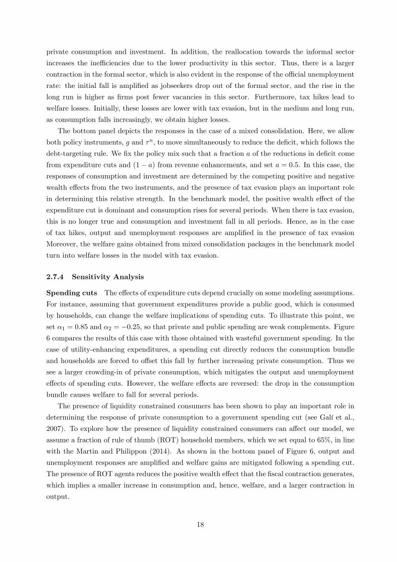
private consumption and investment. In addition, the reallocation towards the informal sector

increases the ineffi ciencies due to the lower productivity in this sector. Thus, there is a larger

contraction in the formal sector, which is also evident in the response of the offi cial unemployment

rate: the initial fall is amplified as jobseekers drop out of the formal sector, and the rise in the

long run is higher as firms post fewer vacancies in this sector. Furthermore, tax hikes lead to

welfare losses. Initially, these losses are lower with tax evasion, but in the medium and long run,

as consumption falls increasingly, we obtain higher losses.

The bottom panel depicts the responses in the case of a mixed consolidation. Here, we allow

both policy instruments, g and τn, to move simultaneously to reduce the deficit, which follows the

debt-targeting rule. We fix the policy mix such that a fraction a of the reductions in deficit come

from expenditure cuts and (1− a) from revenue enhancements, and set a = 0.5. In this case, the

responses of consumption and investment are determined by the competing positive and negative

wealth effects from the two instruments, and the presence of tax evasion plays an important role

in determining this relative strength. In the benchmark model, the positive wealth effect of the

expenditure cut is dominant and consumption rises for several periods. When there is tax evasion,

this is no longer true and consumption and investment fall in all periods. Hence, as in the case

of tax hikes, output and unemployment responses are amplified in the presence of tax evasion

Moreover, the welfare gains obtained from mixed consolidation packages in the benchmark model

turn into welfare losses in the model with tax evasion.

2.7.4 Sensitivity Analysis

Spending cuts The effects of expenditure cuts depend crucially on some modeling assumptions.

For instance, assuming that government expenditures provide a public good, which is consumed

by households, can change the welfare implications of spending cuts. To illustrate this point, we

set α1 = 0.85 and α2 = −0.25, so that private and public spending are weak complements. Figure

6 compares the results of this case with those obtained with wasteful government spending. In the

case of utility-enhancing expenditures, a spending cut directly reduces the consumption bundle

and households are forced to offset this fall by further increasing private consumption. Thus we

see a larger crowding-in of private consumption, which mitigates the output and unemployment

effects of spending cuts. However, the welfare effects are reversed: the drop in the consumption

bundle causes welfare to fall for several periods.

The presence of liquidity constrained consumers has been shown to play an important role in

determining the response of private consumption to a government spending cut (see Galí et al.,

2007). To explore how the presence of liquidity constrained consumers can affect our model, we

assume a fraction of rule of thumb (ROT) household members, which we set equal to 65%, in line

with the Martin and Philippon (2014). As shown in the bottom panel of Figure 6, output and

unemployment responses are amplified and welfare gains are mitigated following a spending cut.

The presence of ROT agents reduces the positive wealth effect that the fiscal contraction generates,

which implies a smaller increase in consumption and, hence, welfare, and a larger contraction in

output.

18

Figure 6: Sensitivity Analysis for Spending Cuts in the Full Model

1 2 3 4 5 6 7 8 9 1 0 1 1

­0 .1 5

­0 .1

­0 .0 5

0

0 .0 5

0 .1

0 .1 5

0 .2

0 .2 5

0 .3

0 .3 5

F IN A L  O U T P U T

1 2 3 4 5 6 7 8 9 1 0 1 1

­2

­1 .5

­1

­0 .5

0

0 .5

O F F IC IA L  U N E M P L O Y M E N T  R A T E

1 2 3 4 5 6 7 8 9 1 0 1 1­0 .4

­0 .2

0

0 .2

0 .4

0 .6

0 .8

1

1 .2

W E L F A R E

W A S T E F U L  S P E N D IN G

U T IL IT Y ­ E N H A N C IN G  S P E N D IN G

Utility-Enhancing Government Spending

1 2 3 4 5 6 7 8 9 1 0 1 1

­0 .1

0

0 .1

0 .2

0 .3

0 .4

0 .5

0 .6

0 .7

0 .8

FIN A L OU TP U T

1 2 3 4 5 6 7 8 9 1 0 1 1

­3 .5

­3

­2 .5

­2

­1 .5

­1

­0 .5

0

0 .5

OFFIC IA L U N E MP LOY ME N T R A TE

1 2 3 4 5 6 7 8 9 1 0 1 1

0 .2

0 .4

0 .6

0 .8

1

1 .2

W E LFA R E

ON LY  OP TIMIZIN G C ON S U ME R S

OP TIMIZIN G A N D  R OT C ON S U ME R S

Rule of Thumb (ROT) Consumers

19

Tax hikes A large body of the literature, initiated by Feldstein (1999), has argued that the

costs of labor taxes can be summarized by the elasticity of taxable income with respect to the net

of tax share. Given the complexity of our theoretical framework, calculating the magnitude of this

elasticity can yield further insights about the effects of tax hikes in the presence of tax evasion

and corruption. We compute the taxable income elasticity by dividing the cumulative response of

taxable income by the cumulative response of the net tax share up to the point that the responses

of tax rates return to zero in the two models. For the benchmark model, the elasticity of taxable

income equals 0.2, while incorporating tax evasion and corruption in the analysis almost doubles

this elasticity to 0.5.8 This is not surprising, given that we are allowing workers to move out of

taxable work, in the formal sector, not only by leaving the workforce but also by working in the

informal sector. Data also suggests higher estimates of the taxable income elasticity in countries

with more tax evasion and corruption. For example, Kleven and Schultz (2014) provide an estimate

for Denmark equal to 0.09 for this elasticity and, using the same methodology, Arrazola et al.

(2014) report a taxable income elasticity equal to 1.5 in Spain.

Of course many of our parameter choices affect the estimated value of the taxable income

elasticity and so, in turn, our conclusions about the effects of tax hikes in a model with tax

evasion and corruption. To investigate this, we first consider the inverse of the intertemporal

elasticity of substitution, η. Smaller values of η imply higher values of the long run elasticity of

taxable income. Accordingly, the higher values of the taxable income elasticity, implied by the

lower η, are associated with higher output and welfare losses, as well as higher unemployment in

the medium and long run, as seen in the top row of Figure 7.

Next, we use alternative values for the inverse of the Frisch elasticity of labor supply, ϕ. The

value of the labor supply elastictity determines the size of the substitution effect and this, in turn,

affects the taxable income elasticity in our model. Higher values of the labor supply elasticity,

meaning lower values of ϕ, are associated with higher values of the taxable income elasticity.

Results presented in the second row of Figure 7 indicate that output losses and medium and long

run unemployment increase with the Frisch elasticity.9

Finally, the incentives to tax evade are also affected by the probability of detection. We

investigate the role of the detection probability in the last row of Figure 7. Intuitively, a higher

probability of detection reduces the output, unemployment, and welfare losses after a consolidation

through tax hikes, since the incentives to reallocate to the informal sector are reduced. However,

this effect is mostly seen in the short and medium run; in the long run, the results are similar for

the different values of ρ.10

8Our estimates are broadly in line with those presented in recent studies that place the value of this elasticityin the (0.2,0.8) range. For a survey of the literature, see Saez et al. (2012).

9Welfare comparisons are more diffi cult when we change η and ϕ because these parameters have a direct impacton the relative weight of consumption and leisure in the utility function.10Since the auditing probability affects the reallocation of workers between sectors, it could also affect the consol-

idation through spending cuts. However, the results under the alternative values of ρ do not change substantiallycompared to the results of the baseline calibration.

20

Figure 7: Sensitivity Analysis for Labor Tax Hikes in the Full Model

2 4 6 8 10

­5

­4

­3

­2

­1

0

F IN A L  O U T P U T

2 4 6 8 10

­50

­40

­30

­20

­10

0

10

20

30

O F F IC IA L  U N E M P L O Y M E N T  R A T E

2 4 6 8 10­1

­0 .8

­0 .6

­0 .4

­0 .2

0

0 .2

W E L F A R E

in t e r t e m p o r a l e la s t ic it y =  1 /2

in t e r t e m p o r a l e la s t ic it y =  1

in t e r t e m p o r a l e la s t ic it y =  1 /0 .5

Intertemporal elasticity of substitution

2 4 6 8 10

­5

­4

­3

­2

­1

0FINAL OUTPUT

2 4 6 8 10

­50

­40

­30

­20

­10

0

10

20

30

OFFICIAL UNEMPLOYMENT RATE

2 4 6 8 10­1

­0.8

­0.6

­0.4

­0.2

0

0.2

WELFARE

Fr isch elasticity=1/2Fr isch elasticity=1/8Fr isch elasticity=1/5Fr isch elasticity=1/0.5

Frisch labor supply elasticity

2 4 6 8 10

­3.5

­3

­2.5

­2

­1.5

­1

­0.5

0FINAL OUTP UT

2 4 6 8 10

­50

­40

­30

­20

­10

0

10

20

OFFICIAL UNE MP LOY ME NT RATE

2 4 6 8 10­0.65

­0.6

­0.55

­0.5

­0.45

­0.4

W E LFARE

detection pr obability=2%detection pr obability=1%detection pr obability=3%

Detection probability

21

Table 2: Calibrated Values

Consolidation Volume - 2010 (% GDP) 7.8%Consolidation Volume - 2015 (% GDP) 18.5%Expenditure Share in Policy Mix 0.60

3 Policy Evaluation

We employ our DSGE model to analyze the effects of the recent consolidation packages imple-

mented in Greece. Using the information in OECD (2012), we adjust the size of the consolidation

to match the reduction in the deficit-to-GDP ratio implemented in 2010 and also replicate the an-

nounced consolidation volumes in the long run. Table 2 reports the consolidation in 2010 and the

intended consolidation to be implemented by 2015. In order to replicate the actual consolidation

packages, we allow both instruments to move simultaneously, again using OECD (2012) to fix the

relative contribution of the two instruments.11

The simulation results are shown in Figure 8. Despite the substantial use of expenditure cuts,

we see that tax evasion increases. With the use of tax hikes in the consolidation mix, the direct

incentive to produce in the informal sector dominates the effi ciency gains from producing in the

formal sector, leading to a reallocation towards the informal sector. The model predicts sizeable

and persistent output losses, unemployment increases in the long run and welfare losses following

the consolidation packages.

4 Conclusions

A New Keynesian DSGE model with involuntary unemployment and an informal sector demon-

strates that the presence of the latter amplifies the contractionary effects of labor tax hikes, while

mitigates the effects of expenditure cuts. It also shows that the instrument used to achieve fiscal

consolidation affects the incentives of agents to produce in the informal sector. Spending cuts

reduce the size of the informal economy, while tax hikes increase it.

We also analyze how current fiscal consolidation plans in Greece affect tax evasion, output,

unemployment, and welfare. The model predicts increasing levels of tax evasion during the consol-

idation, and prolonged output and welfare losses. Greece suffers heavy losses due to the severity of

the austerity package implemented. Furthermore, the welfare costs of these consolidations would

have been smaller if tax evasion had been reduced. Hence, reforms aimed at fighting tax evasion

should go hand-in-hand with austerity measures in order to mitigate the welfare costs of fiscal

consolidations.

Our exercise is the first attempt to analyze the effects of fiscal consolidation in the presence of

tax evasion. Since the model is stylized, it leaves out important aspects of reality that could affect

our conclusions. For example, in our economy there is a representative household, and so we cannot

assess the effects of tax evasion on income inequality. Also, we consider only cuts in government

consumption expenditures and not in other items of the government budget. Furthermore, our

11See the table on p.138 of OECD (2012).

22

Figure8:SimulationofFiscalConsolidationMix

12

34

56

78

­20

­15

­10­5

FIN

AL 

OU

TPU

T

12

34

56

78

­40

­30

­20

­100

OFF

ICIA

L U

NE

MP

LOY

ME

NT 

RA

TE

12

34

56

78

2468

UN

DE

RG

RO

UN

D O

UTP

UT

12

34

56

78

­0.6

­0.4

­0.20

0.2

0.4

WE

LFA

RE

12

34

56

78

­10010203040

FIS

CA

L IN

STR

UM

EN

TS

gov

.spe

ndin

gla

bor 

tax 

rate

12

34

56

78

­18

­16

­14

­12

­10­8

DE

FIC

IT­T

O­G

DP

 RA

TIO

23

model does not allow for evasion of consumption taxes, which is an important component of tax

evasion in southern European countries. We leave these extensions for future research.

24

References

[1] Alesina A., C. Favero and F. Giavazzi, 2013, ‘The Output Effect of Fiscal Consolidations’,

Working Papers 478, IGIER, Bocconi University.

[2] Bermperoglou D., E. Pappa and E. Vella, 2014, ‘Spending Cuts and Their Effects on Output,

Unemployment and the Deficit’, Unpublished Manuscript.

[3] Boeri T. and P. Garibaldi, 2007, ‘Shadow Sorting,’NBER International Seminar on Macro-

economics 2005, MIT Press, 125-163.

[4] Brückner, M. and E. Pappa, 2012, ‘Fiscal Expansions, Unemployment, and Labor Force

Participation: Theory and Evidence’, International Economic Review, 53(4), 1205-1228.

[5] Buehn A. and F. Schneider, 2012, ‘Corruption and the Shadow Economy: Like Oil and

Vinegar, Like Water and Fire?’, International Tax and Public Finance, 19(1), 172-194.

[6] Busato F. and B. Chiarini, 2004, ‘Market and Underground Activities in a Two-Sector Dy-

namic Equilibrium Model’, Economic Theory, 23(4), 831-861.

[7] Calvo, G. A., 1983, ‘Staggered Prices in a Utility-Maximizing Framework,’Journal of Mon-

etary Economics, 12(3), 383-398.

[8] Campolmi A. and S. Gnocchi, 2014, ‘Labor Market Participation, Unemployment and Mon-

etary Policy’, Bank of Canada Working Paper No. 2014/9.

[9] Colombo E., L. Onnis and P. Tirelli, 2014, ‘Shadow Economies at Times of Banking Crises:

Empirics and Theory’, Journal of Banking and Finance, forthcoming.

[10] Erceg, C. and J. Lindé, 2013, ‘Fiscal Consolidation in a Currency Union: Spending Cuts vs.

Tax Hikes,’Journal of Economic Dynamics and Control, 37(2), 422-445.

[11] Fugazza M. and J.-F. Jacques, 2004, ‘Labor Market Institutions, Taxation and the Under-

ground Economy,’Journal of Public Economics, 88, 395-418.

[12] Galí, J., J. D. López-Salido and J. Vallés, 2007, ‘Understanding the Effects of Government

Spending on Consumption,’Journal of the European Economic Association, 5(1), 227-270.

[13] Gestha, 2014, ‘La Economía Sumergida Pasa Factura. El Avance del Fraude en España

Durante la Crisis’, Madrid, enero de 2014.

[14] Hansen G., 1985, ‘Indivisible Labor and the Business Cycle,’Journal of Monetary Economics,

16, 309-27.

[15] Hansen L. P., and K. Singleton, 1983, ‘Stochastic Consumption, Risk Aversion and the

Temporal Behavior of Asset Returns’, Journal of Political Economy, 91, 249-265.

[16] Martin J., 1996, ‘Measures of Replacement Rates for the Purpose of International Compari-

son: A Note’, OECD Economic Studies, 26(1), 98-118.

25

[17] Martin, P. and T. Philippon, 2014, ‘Inspecting the Mechanism: Leverage and the Great

Recession in the Eurozone,’Unpublished Manuscript.

[18] OECD, 2012, Restoring Public Finances, 2012 Update, OECD Publishing.

http://dx.doi.org/10.1787/9789264179455-en

[19] Orsi R., D. Raggi and F. Turino, 2014, ‘Size, Trend, and Policy Implications of the Under-

ground Economy’, forthcoming in the Review of Economic Dynamics.

[20] Pappadà, F. and Y. Zylberberg, 2014, ‘Austerity Plans and Tax Evasion: Theory and Evi-

dence from Greece’, Unpublished Manuscript.

[21] Peracchi F. and E. Viviano, 2004, ‘An Empirical Micro Matching Model with an Application

to Italy and Spain’, Temi di discussione No. 538, Banca d Italia.

[22] Perotti, R., 1996, ‘Fiscal Consolidation in the Europe: Composition Matters’, American

Economic Review Papers and Proceedings, 86(2), 105-110.

[23] Ravn, M. O., 2008, ‘The Consumption-Tightness Puzzle’, NBER Chapters, NBER Interna-

tional Seminar on Macroeconomics 2006, 9-63.

[24] Restrepo-Echavarria P., 2014, ‘Macroeconomic Volatility: The Role of the Informal Economy,’

European Economic Review, 70, 454-469.

26

5 Derivations

5.1 Household’s maximization problem

We can write in full the Lagrangean for the representative household’s maximization problem.

Firstly, we can incorporate the composition of the household, as well as the definition of the total

effective consumption bundle, directly into the utility function of the household. Then, we can

plug the definition of the matches mjt = ψhjt u

jt into the law of motion of employment in each

sector, and also replace it in the budget constraint using the law of motion of private capital.

Then we are left with 3 constraints, and the following Lagrangean:

L = E0

∞∑t=0

βt

{[α1(ct)

α2 + (1− α1)(gt)α2 ]

1−ηα2

1− η + Φ

[1− ut − nFt − nIt

]1−ϕ1− ϕ

−λct[(1 + τ ct)ct + kt+1 − (1− δ)kt +

ω

2

(kt+1

kt− 1

)2

kt +Bt+1πt+1

Rt− rtkt

−(1− τnt )wFt nFt − wIt nIt −$(1− st)ut −Bt −Πp

t + Tt

]−λnF t

[nFt+1 − (1− σF )nFt − ψhFt (1− st)ut

]−λnI t

[nIt+1 − (1− ρ− σI)nIt − ψhIt stut

]}(28)

The controls are ct, kt+1, Bt+1, nFt+1, nIt+1, ut and st. The first order conditions are:

[wrt ct]

cc(1−η−α2)t α1c

(α2−1)t − λct(1 + τ ct) = 0 (29)

[wrt kt+1]

λct

[1 + ω

(kt+1

kt− 1

)]− βEtλct+1

[1− δ + rt+1 +

ω

2

((kt+2

kt+1

)2

− 1

)]= 0 (30)

[wrt Bt+1]

−λct1

Rt+ βEtλct+1

1

πt+1= 0 (31)

[wrt nFt+1]

−λnF t − βEt[Φl−ϕt+1 − λct+1(1− τnt+1)wFt+1 − λnF t+1(1− σF )

]= 0 (32)

[wrt nIt+1]

−λnI t − βEt[Φl−ϕt+1 − λct+1w

It+1 − λnI t+1(1− ρ− σI)] = 0 (33)

27

[wrt ut]

−Φl−ϕt + λct$ + λnF tψhFt (1− st) + λnI tψ

hIt st = 0 (34)

[wrt st]

−λnF tψhFt ut + λnI tψhIt ut − λct$ = 0 (35)

Equations (29)-(31) are the arbitrage conditions for the returns to consumption, private capital

and bonds. Equations (32) and (33) relate the expected marginal value from being employed in

the each sector to the wage, accounting for the income tax in the regular sector, the utility loss

from the reduction in leisure, and the continuation value, which depends on the separation prob-

ability. Equation (34) states that the value of being unemployed (rather than enjoying leisure),

λct$, should equal the marginal utility from leisure minus the expected marginal values of being

employed in each sector, weighted by the respective job finding probabilities and shares of jobseek-

ers. Equation (35) is an arbitrage condition according to which the choice of the share, st, is such

that the expected marginal values of being employed, weighted by the job finding probabilities,

are equal across the two sectors.

We can define the marginal value to the household of having an additional member employed

in the two sectors, as follows:

V hnF t ≡

∂L∂nFt

= λctwFt (1− τnt )− Φl−ϕt + (1− σF )λnF t (36)

= λctwFt (1− τnt )− Φl−ϕt + (1− σF )βEt(V

hnF t+1)

V hnI t ≡

∂L∂nIt

= λctwIt − Φl−ϕt + (1− ρ− σI)λnI t (37)

= λctwIt − Φl−ϕt + (1− ρ− σI)βEt(V h

nI t+1)

where the second equalities come from equations (32) and (33) respectively.

5.2 Derivation of the resource constraint

Consider the household’s budget constraint:

(1 + τ ct)ct + it +Bt+1πt+1

Rt≤ rtkt + (1− τnt )wFt n

Ft + wIt n

It +$uFt +Bt + Πp

t − Tt (38)

Recall the government’s budget constraint:

Bt+1πt+1

Rt−Bt = DFt

Plugging this into (38):

(1 + τ ct)ct + it +DFt ≤ rtkt + (1− τnt )wFt nFt + wIt n

It +$uFt + Πp

t − Tt (39)

28

Recall also the definition of the deficit:

DFt = gt +$uFt −[(τnt + τ st )w

Ft n

Ft + τ ctct + Tt

]− ργpxt xt

Plugging this directly into equation (39):

(1 + τ ct)ct + it + gt +$uFt −[τ ctct + (τnt + τ st )w

Ft n

Ft + Tt

]− ργpxt xt =

rtkt + (1 − τnt )wFt nFt + wIt n

It + $uFt + Πp

t − Tt

Cancelling out the taxes and unemployment benefits, we have:

ct + it + gt − ργpxt xt = rtkt + (1 + τ st )wFt n

Ft + wIt n

It + Πp

t (40)

Recall now that (i) the price of the final good is normalised to 1, (ii) the retail firms turn xt units

of the intermediate good into yt units of the final good, and (iii) the differentiated retail goods

are costlessly aggregated into the final consumption good. Then by definition, the profit from the

retail firm can be written as:

Πpt = yt − pxt xt (41)

Substituting this into equation (40), we obtain:

ct + it + gt = rtkt + (1 + τ st )wFt n

Ft + wIt n

It + yt − (1− ργ)pxt xt (42)

The price of the intermediate good, pxt , is determined by the zero-profit condition of the interme-

diate goods producing firm. That is, it satisfies:

(1− ργ) pxt xt︸ ︷︷ ︸Revenue of intermediate firms

−[(1 + τ st )w

Ft n

Ft + wIt n

It + rtkt + κFυFt + κIυIt

]︸ ︷︷ ︸Costs of intermediate firms

= 0

Plugging this into equation (42):

ct + it + gt = rtkt + (1τ st )wFt n

Ft

+wIt nIt + yt −

[(1 + τ st )w

Ft n

Ft + wIt n

It + rtkt + κFυFt + κIυIt

](43)

Cancelling terms we have:

ct + it + gt = yt −(κFυFt + κIυIt

)(44)

Rearranging terms we get the final expression:

yt = ct + it + gt + κFυFt + κIυIt

29

5.3 Derivation of the wages

For each sector j = F, I the Nash bargaining problem is to maximize the weighted sum of log

surpluses:

maxwjt

{(1− ϑj) lnV h

njt + ϑj lnV fnjt

}where V h

njtand V f

njtare defined as:

V hnF t = λctw

Ft (1− τnt )− Φl−ϕt + (1− σF )λnF t (45)

V hnI t = λctw

It − Φl−ϕt + (1− ρ− σI)λnI t (46)

V fnF t≡ ∂Q

∂nFt= (1− ργ) pxt (1− αF )

xFtnFt− (1 + τ st )w

Ft +

(1− σF )κF

ψfFt(47)

V fnI t≡ ∂Q

∂nIt= (1− ργ) pxt (1− αI)x

It

nIt− wIt +

(1− ρ− σI)κI

ψfIt(48)

The first order conditions of these optimization problems are:

ϑF (1 + τ st )VhnF t = (1− ϑF )λct(1− τnt )V f

nF t(49)

ϑIV hnI t = (1− ϑI)λctV f

nI t(50)

Plugging the expressions for the value functions into these FOCs, we can rearrange to find ex-

pressions for wFt and wIt . Using (45), (47) and (49), we can solve for w

Ft , which yields:

wFt =(1− ϑF )

(1 + τ st )

((1− ργ) pxt (1− αF )

xFtnFt

+(1− σF )κF

ψfFt

)+

ϑF

λct(1− τnt )

(Φl−ϕt −(1−σF )λnF t

)(51)

Similarly using (46), (48) and (50), we can solve for wIt , which yields:

wIt = (1−ϑI)(

(1− ργ) pxt (1− αI)xIt

nIt+

(1− ρ− σI)κI

ψfIt

)+ϑI

λct

(Φl−ϕt − (1−ρ−σI)λnI t

)(52)

30