Math 125: Calculus II - Dr. Loveless

Today

Syllabus/Intro

Section 4.9 - antiderivatives

Week 1 assignments Closing time is always 11pm.

- HW 1A,1B closes Wed - HW 1C closes Fri

(covers 4.9, 5.1, and 5.2) Expect 6-8 hrs of work, start today!

Essential Course Info My Course Website: math.washington.edu/~aloveles/ Homework Log-In (use UWNetID): webassign.net/washington/login.html Directions for Webassign code purchase: math.washington.edu/webassign Math Department 125 Course Page: math.washington.edu/~m125/

First week to do list 1. Read 4.9, 5.1, 5.2, and 5.3 of the book. Start attempting HW. 2. Print off the “worksheets” and bring them to quiz sections.

What we will do in this course: We learn integral calculus which provides the essential tools for engineering, science and economics. 1. Ch. 5 – Defining the Integral

- Def’n and basic techniques

2. Ch. 6 – Basic Integral Applications - Areas, Volumes - Average Value - Measuring Work

3. Ch. 7 – Integration Techniques - by parts, trig, trig sub, partial frac.

4. Ch. 8-9 – More Applications

- Arc Length, Center of Mass - Differential Equations

5. Practicing Algebra, Trig and Precalc Students often say: The hardest part of calculus is you have to know all your precalculus, and they are right. Improving your algebra, trig and precalculus skills will be one of the best benefits you will gain from this course. (Arguably as valuable as the course content itself). You will use these skills often in your other courses at UW, so embrace, practice, and hone your precalculus skills.

Entry Task: Differentiate

1. 𝐹(𝑥) =7

𝑥10 − 5√𝑥3 + 4ln (𝑥)

2. 𝐺(𝑥) = 𝑒6𝑥 + 5 tan(𝑥) + 𝜋

3. 𝐻(𝑥) = 2 tan−1(𝑥) − 𝑒

4. 𝐽(𝑥) = 𝑥3 cos(4𝑥) + ln(2)

4.9 Antiderivatives

Def’n: If g(x) = f’(x), then we say

g(x) = “the derivative of f(x)”, and

f(x) = “an antiderivative of g(x)”

Example:

Give an antiderivative of

𝑔(𝑥) = 𝑥2.

Examples (you do):

Find the general antiderivative of

1. 𝑓(𝑥) = 𝑥6

2. 𝑔(𝑥) = cos(𝑥) +1

𝑥+ 𝑒𝑥 +

1

1+𝑥2

3. ℎ(𝑥) =5

√𝑥+ √𝑥23

4. 𝑟(𝑥) =𝑥−3𝑥2

𝑥3

Initial Conditions

There is no way to know what “C” is

unless we are given additional

information. Such information is

called an initial condition.

Example: 𝑓’(𝑥) = 𝑒𝑥 + 4𝑥 and

𝑓(0) = 5

Find 𝑓(𝑥).

Example: 𝑓′′(𝑥) = 15√𝑥, and

𝑓(1) = 0, 𝑓(4) = 1 Find 𝑓(𝑥).

Example: Ron steps off the 10 meter high dive at his local pool. Find a formula for his height above the water. (Assume his acceleration is a constant 9.8 m/s2 downward)

5.1 Defining Area Calculus is based on limiting processes that “approach” the exact answer to a rate question. In Calculus I, you defined f’(x) = `slope of the tangent at x’

= limℎ→0

𝑓(𝑥 + ℎ) − 𝑓(𝑥)

ℎ

In Calculus II, we will see that antiderivatives are related to the area `under’ a graph

= lim𝑛→∞

∑ 𝑓(𝑥𝑖∗)∆𝑥

𝑛

𝑖=1

Calc. I Visual: Calc. II Visual:

Riemann sums set up: We build a procedure to get better and better approximations of the area “under” 𝑓(𝑥). 1. Break into n subintervals.

∆𝑥 = 𝑏−𝑎

𝑛 and 𝑥𝑖 = 𝑎 + 𝑖∆𝑥

2. Draw n rectangles.

Area of each rectangle = (height)(width) = 𝑓(𝑥𝑖

∗)∆𝑥

3. Add up rectangle areas.

Example: Approx. the area under 𝑓(𝑥) = 𝑥3 from x = 0 to x = 1 using n = 3 subdivisions and right-endpoints to find the heights.

You do: Approx. the area under 𝑓(𝑥) = 𝑥3 from x = 0 to x = 1 using n = 4 subdivisions and left-endpoints to find the heights.

I did this again with 100 subdivisions, then 1000, then 10000. Here is a summary of my findings:

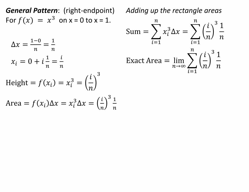
General Pattern: (right-endpoint) For 𝑓(𝑥) = 𝑥3 on x = 0 to x = 1.

∆𝑥 =1−0

𝑛=

1

𝑛

𝑥𝑖 = 0 + 𝑖1

𝑛=

𝑖

𝑛

Height = 𝑓(𝑥𝑖) = 𝑥𝑖3 = (

𝑖

𝑛)

3

Area = 𝑓(𝑥𝑖)∆𝑥 = 𝑥𝑖3∆𝑥 = (

𝑖

𝑛)

3 1

𝑛

Adding up the rectangle areas

Sum = ∑ 𝑥𝑖3∆𝑥

𝑛

𝑖=1

= ∑ (𝑖

𝑛)

3 1

𝑛

𝑛

𝑖=1

Exact Area = lim𝑛→∞

∑ (𝑖

𝑛)

3 1

𝑛

𝑛

𝑖=1

Definition of the Definite Integral We define the exact area “under” f(x) from x = a to x = b curve to be

lim𝑛→∞

∑ 𝑓(𝑥𝑖)∆𝑥

𝑛

𝑖=1

,

where ∆𝑥 = 𝑏−𝑎

𝑛 and

𝑥𝑖 = 𝑎 + 𝑖∆𝑥. We call this the definite integral of f(x) from x = a to x = b, and we write

∫ 𝑓(𝑥)𝑑𝑥𝑏

𝑎

= lim𝑛→∞

∑ 𝑓(𝑥𝑖)∆𝑥

𝑛

𝑖=1

Example: Write down this definition

for the function 𝑓(𝑥) = √𝑥 on the interval 𝑥 = 5 to 𝑥 = 7.