Physica A 390 (2011) 1841–1852

Contents lists available at ScienceDirect

Physica A

journal homepage: www.elsevier.com/locate/physa

First passage time statistics of Brownian motion with purely timedependent drift and diffusionA. Molini a,b,∗, P. Talkner c, G.G. Katul b,a, A. Porporato a,b

aDepartment of Civil and Environmental Engineering, Pratt School of Engineering, Duke University, Durham, NC, USA

bNicholas School of the Environment, Duke University, Durham, NC, USA

cInstitut für Physik, Universität Augsburg, Augsburg, Germany

a r t i c l e i n f o

Article history:

Received 2 September 2010Received in revised form 23 December 2010Available online 17 February 2011

Keywords:

Brownian motionTime-dependent drift and diffusionAbsorbing barrierSnowmelt

a b s t r a c t

Systems where resource availability approaches a critical threshold are common tomany engineering and scientific applications and often necessitate the estimation of firstpassage time statistics of a Brownian motion (Bm) driven by time-dependent drift anddiffusion coefficients. Modeling such systems requires solving the associated Fokker-Planck equation subject to an absorbing barrier. Transitional probabilities are derivedvia the method of images, whose applicability to time dependent problems is shownto be limited to state-independent drift and diffusion coefficients that only dependon time and are proportional to each other. First passage time statistics, such as thesurvival probabilities and first passage timedensities are obtained analytically. The analysisincludes the study of different functional forms of the time dependent drift and diffusion,including power-law time dependence and different periodic drivers. As a case study ofthese theoretical results, a stochastic model of water resources availability in snowmeltdominated regions is presented, where both temperature effects and snow-precipitationinput are incorporated.

© 2011 Elsevier B.V. All rights reserved.

1. Introduction

A wide range of geophysical and environmental processes occur under the influence of an external time-dependentand random forcing. Climate-driven phenomena, such as plant productivity [1], steno-thermal populations dynamics [2],crop production [3], the alternation between snow-storage and melting in mountain regions [4,5], the life cycle oftidal communities [6–8], and water-borne diseases outbreaks [9,10] offer a few such examples. In particular, severalenvironmental systems can be described by state variables representing the availability of a resource whose dynamics isforced by diverse environmental factors and climatic oscillations. Elevated regions water availability — mainly originatingfrom the melting of snow masses accumulated during the winter period (under the forcing of increasing temperatures),and precipitation (moving from the solid precipitation to the rainfall regime) — offers a relevant case study (presented inSection 4). All of these processes are now receiving increased attention in several branches of ecology, climate sciences andhydrology, due to their inherent sensitivity to climatic variability.

Analogous dynamical patterns can be found in slowly-driven, non-equilibrium systems with self organized criticality(SOC),where thedensity of potentially relaxable sites in the systemcanbedescribed via a randomwalkwith time-dependentdrift and diffusion terms [11–13]. In these systems, the time dependence in the diffusion term derives from a gradual

∗ Corresponding author at: Department of Civil and Environmental Engineering, Pratt School of Engineering, Duke University, Durham, NC, USA.Tel.: +1 919 668 3809; fax: +1 919 684 8741.

E-mail address: annalisa.molini@duke.edu (A. Molini).

0378-4371/$ – see front matter© 2011 Elsevier B.V. All rights reserved.doi:10.1016/j.physa.2011.01.024

1842 A. Molini et al. / Physica A 390 (2011) 1841–1852

decrease of susceptible sites, so that sites availability acts on the directionality and pathways (drift term) of the ‘‘avalanches’’until diffusion ‘‘kills’’ all the activity in the system [14, pp. 120–131]. Similar dynamics occur in systems displaying stochasticresonance, where noise becomes modulated by an external periodic forcing (see [15–18] and references therein).

In many instances, the above-mentioned processes are restricted to the positive semi-axis or to the time at which acertain critical threshold is reached, and are represented by a Fokker–Planck (FP) equation with an absorbing barrier. Themain focus here is on the first passage time statistics of the process, such as the survival probabilities and the first passagetime densities. In the following, a brief review of the general properties of the time-dependent drift and diffusion processeswith an absorbing barrier is presented. For constant drift and diffusion, the conditional probabilities are usually obtained viathemethod of images due to Lord Kelvin (see [19, p. 340]). The applicability of thismethod to the solution of time-dependentproblems and its limitations are discussed and a necessary and sufficient criterion is formulated in Section 2.2. The analysis isthen extended to different functional forms of the time-dependent drift and diffusion terms. Section 3.1 shows the analyticalresults for the first passage time statistics for a power-law time dependent drift and diffusion, while time-periodic driversare analyzed in Section 3.2 (see [20–22] and references therein, for a more comprehensive review of periodically-drivenstochastic processes). Finally, in Section 4, we present a stochastic model of the total mountain water equivalent duringthe apex phase of the melting season, incorporating both temperature effects and snow-precipitation input in the form of apower-law time-dependent Bm with an absorbing boundary.

2. Modeling framework

When a time-dependent random forcing is the dominant driver of the dynamics, a general representation for the statevariable x(t) can be formulated in the form of a stochastic differential equation given by

dx(t) = µ(t) dt + σ (t) dW (t) (1)where µ(t) and σ (t) are purely time-dependent drift and diffusion terms, and W (t) is a Wiener process with independentand identically Gaussian distributed (i.i.d.) increments W (t) − W (s) ∼ N (0, t − s) for all t � s � 0. By assuming t0 = 0,the solution of (1) takes the form

x(t) = x0 +�

t

0µ(s)ds +

�t

0[σ (s)dW (s)] (2)

where t is time and x0 = x(0) can be either a random or a non-random initial condition independent of W (t) − W (0). Theassociated FP equation describing the evolution of the probability density function (pdf) of x(t) can be expressed as

∂p(x, t|x0)∂t

= −µ(t)∂p(x, t|x0)

∂x+ 1

2σ 2(t)

∂2p(x, t|x0)

∂x2, (3)

where p(x, t|x0) is the transition pdf with initial condition δ(x − x0) at t0. Eq. (3) can also be expressed as a continuityequation for probability

∂

∂tp(x, t|x0) = − ∂

∂xj(x, t|x0), (4)

where

j(x, t|x0) = µ(t)p(x, t|x0) − 12σ 2(t)

∂p(x, t|x0)∂x

, (5)

is the probability current (or flux) and p(x, t|x0) is the conditional probability. The solution of the FP equation in (3), is usuallyapproached numerically (see for e.g., [23]). Whether this equation is analytically solvable for different functional forms ofµ(t) and σ (t) with an absorbing boundary, and whether these solutions can be applied in the study of the first passagestatistics at such boundary is the main focus of this work. Case studies that employ these solutions are also presented.

2.1. Solution with natural boundaries

Consider first the solution of the FP equation (3) in the unbounded case. Given that the drift and diffusion coefficientsdepend only on time, the parabolic Eq. (3) can still be reduced to a constant-coefficient equation of the form

∂p(z, τ )

∂τ= ∂2

p(z, τ )

∂z2(6)

by transforming the original variables x and t into

τ = 12

�σ 2(t)dt + A (7)

and

z = x −�

µ(t)dt + B (8)

A. Molini et al. / Physica A 390 (2011) 1841–1852 1843

where A and B are generic constants. The solution with natural boundaries is then p(z, τ ) = 12√

πτexp

�− z

2

4τ

�[24]. Hence,

given the initial conditionp(x, 0|x0) = δ(x − x0), (9)

the following normalized solution for an unrestricted process, starting from x0, can be obtained as

pu(x, t|x0) = 12√

πS(t)exp

�− (x − x0 − M(t))2

4S(t)

�, (10)

where, assuming the integrability of µ(t) and σ (t),

M(t) =�

t

0µ(s)ds (11)

and

S(t) = 12

�t

0σ 2(s)ds. (12)

It should be noted that the transformation in Eqs. (8) and (7) also applies to any boundary condition imposed at a finiteposition. Therefore, as will be seen, it is not directly helpful in solving first passage time problems, as in that case it wouldlead to a problem withmoving absorbing boundary conditions.

2.2. First passage time distributions

For a Bm process commencing at a generic position x0 at t = 0, the time at which this process reaches an arbitrarythreshold a for the first time (first passage time) is itself a random variable whose statistics are fundamental in manybranches of science such as chemistry, neural-sciences and econometrics. In the following, it is assumed that the processis starting at a certain state x0 > 0 and that it is bounded to the positive semi-axis via an absorbing barrier x = 0.This hypothesis does not imply any loss of generality, considering that the solution of Eq. (3) with an absorbing boundarycondition only depends on the distance of the initial point x0 from the threshold, but not separately on x0 and the thresholdposition. Eq. (3) is then solved with the boundary condition

p(0, t) = 0, (13)and the additional condition of x = +∞ being a natural boundary to ensure that j(+∞, t|x0) = 0. For such a system, thesurvival probability F(t|x0) is defined as the probability of the process trajectories not absorbed before time t , i.e.

F(t|x0) =� +∞

0p(x, t|x0) dx (14)

and the first passage probability density g(t|x0) is either the ‘‘rate of decrease’’ in time of F

g(t|x0) = − ∂

∂tF(t|x0) . (15)

or, alternatively, the negative probability current at the boundary

g(t|x0) = σ 2(t)

2∂

∂xp(x, t|x0)

����x=0

, (16)

since p(0, t|x0) = 0 from (13).

2.3. Method of images in time-dependent systems

When the drift and diffusion terms are independent of t and x, Eq. (3) with absorbing boundaries can be readily solvedby themethod of images, often adopted in problems of heat conduction and diffusion [25,26,14,27]. This method can also beused for solving boundary-value problems for a Bm with particular forms of time-dependent drift and diffusion. The basicpremise of this method is that given a linear PDE with a point source (or sink) subject to homogeneous boundary conditionsin a finite domain, its general solution can be obtained as a superposition of many ‘free space’ solutions (i.e. disregarding theboundary conditions) for a number of virtual sources (i.e. outside the domain) selected so as to obtain the correct boundarycondition. The image source (or sink) is placed as mirror image of the original source (or sink) from the boundary with astrength or intensity selected to match the boundary condition.

Consider Eq. (3) with the conditions (9) and (13). To solve this problem with the method of images, the barrier at 0 isreplaced by a mirror source located at a generic point x = y, with y < 0 such that the solutions of the Fokker–Planckequation emanating from the original and mirror sources exactly compensate each other at the position of the barrier ateach instant of time [14]. This implies the initial conditions in (9) must now be modified to

p(x, 0) = δ(x − x0) − exp (−η) δ(x − y), (17)

1844 A. Molini et al. / Physica A 390 (2011) 1841–1852

where η determines the strength of the mirror image source. Due to the linearity of the FP equation, the solution in thepresence of the initial condition (17) is the superposition of elementary solutions

p(x, t|x0) = pu(x, t|x0) − exp (−η) pu(x, t|y). (18)Since the condition (13) requires that p(0, t|x0) = 0, one obtains that

(M(t) + x0)2

4S(t)= η + (M(t) + y)2

4S(t)(19)

for all t > 0. By assuming t = 0, we have x20 = y2 and recalling that y < 0, the resulting image position is−x0. This, inserted

again in Eq. (19), yieldsM(t)

S(t)= η

x0= q, (20)

where the constant q is analogous to the Péclet number of the process—i.e. the ratio between the advection and diffusionrates [14].

After differentiating (20) with respect to t , it is seen that the method of images requires that the drift and the diffusionterms be proportional to each other. Namely, the intensity η of the image source must be constant in time. In fact, only inthis case it is still possible to transform the original time scale into a new one, for which the transformed process is governedby time-independent drift and diffusion terms. Hence, writing the drift and diffusion terms as

µ(t) = kh(t) andσ 2

2= lh(t), (21)

the associated FP equation is

∂p

∂t= h(t)

�−k

∂

∂x+ l

∂2

∂x2

�p. (22)

Transforming the original time t variable in

τ̃ =�

t

0h(s)ds (23)

Eq. (22) finally becomes

∂p

∂τ̃=

�−k

∂

∂x+ l

∂2

∂x2

�p. (24)

This condition is valid for any time-dependent diffusionwhen the drift is identically vanishing. Assuming the proportionalityin (20) between µ(t) and σ (t), the general solution for (3) under conditions (9) and (13) can be written as

p(x, t|x0) = 12√

πS(t)

�exp

�− (x − x0 − M(t))2

4S(t)

�− exp (−x0q) exp

�− (x + x0 − M(t))2

4S(t)

��, (25)

provided M(t) = qS(t). Substituting for constant drift and diffusion in (25) one recovers the well-known solution for abiased Bm [25]

p(x, t|x0) = 1√2π

√σ 2t

�exp

�− (x0 − x + µt)2

2σ 2t

�− exp

�−2x0µ

σ 2

�exp

�(x + x0 − µt)2

2σ 2t

��(26)

with survival function F(t|x0) given by

F(t|x0) = Φ

�µt + x0

σ√t

�− exp

�−2x0µ

σ 2

�Φ

�µt − x0

σ√t

�, (27)

where Φ is the standard normal integral, and first passage time distribution

g(t|x0) = x0

σ√2π t3/2

exp�− (x0 + µt)2

2σ 2t

�. (28)

Eq. (28) is theWald (or inverse Gaussian) density function, that for a zero drift becomes of order t−3/2 as t → +∞ (the firstpassage time has no finite moments for pure diffusion).

Similarly, the solution to the FP in Eq. (3) with a reflecting boundary at x = 0 can be obtained by the method of imagesprovided that drift and diffusion are proportional to each other. The solution then becomes

p(x, t|x0) = 12√

πS(t)

�exp

�− (x − x0 − M(t))2

4S(t)

�+ exp (−x0q) exp

�− (x + x0 − M(t))2

4S(t)

�

− 12M(t)

S(t)exp

�xη

x0

� �1 − erf

�x + x0 + M(t)

2√S(t)

���, (29)

A. Molini et al. / Physica A 390 (2011) 1841–1852 1845

with 12

�1 − erf

�x+x0+M(t)

2√S(t)

��being the Q -function representing the tail probability of a Gaussian distribution. Eq. (29)

generalizes the solution in Ref. [25] for a Bm with constant drift and diffusion and a reflecting boundary at 0.

3. Time dependent drift and diffusion

3.1. Power-law time dependence

As a first example of Bm with purely time-dependent drivers, the case of an unbiased diffusion (q = 0) and power-lawtime dependent diffusion term σ 2(t) = 2Atα and α > −1 are considered. For this process, the conditional probabilityp(x, t|x0) with absorbing barriers at 0, takes on the form

p(x, t|x0) =√1 + α

2√Aπ

t−(α+1)

�exp

�− t

−(α+1)(x − x0)2(1 + α)

4A

�− exp

�− t

−(α+1)(x + x0)2(1 + α)

4A

��, (30)

while the survival function becomes

F(t|x0) = erf

�x0(1 + α)

12

2√A

t− α+1

2

�

. (31)

Fig. 1(a) shows the conditional probability (30) at a fixed time instance t = 15 time steps for A = 15, x0 = 50, andα = −0.1 (bold line) 0.5 (thin line), and 1 (dotted line). Given the asymptotic properties of the error function [28], thelong-time behavior of F(t|x0) is then ∼ x0(1+α)1/2

2√A

t− α+1

2 , recovering for α = 0 the −1/2 tail decay of an unbiased constantdiffusion (see Fig. 1(b)). Also, by differentiating Eq. (31), one obtains

g(t|x0) = x0

2�

Aπ(α+1)3 t

(3+α)/2exp

�−x0(α + 1)t−(α+1)

4A

�(32)

whose tail behaves as ∼ t−

�3+α2

�

. Hence, Eq. (32) is an inverse Gaussian distribution — that for α = 0 becomes an inverseGamma distribution with shape parameter 1/2 [29, pp. 284–285]. These solutions characterize inter-arrival times betweenintermittent events when a system displays sporadic randomness [30–32].

The solutions in the case of proportional power-law diffusion and drift can be derived in an analogous manner. Forµ(t) = qAt

α and σ (t) =√2A1/2

tα/2, the conditional probability p(x, t|x0) takes the form

p(x, t|x0) =√

α + 1t−(α+1)/2

2√Aπ

exp

−(1 + α)t−(α+1)

�−x + Aqt

1+α

1+α+ x0

�2

4A

− exp

−qx0 −(1 + α)t−(α+1)

�x − Aqt

1+α

1+α+ x0

�2

4A

(33)

and the survival function, now incorporating the drift contribution, can be written as

F(t|x0) = Φ

�

t− (α+1)

2

�Aqt

α+1 + x0 + x0α�

2√A(α + 1)

�

− exp (−qx0) Φ

�

t− (α+1)

2

�Aqt

α+1 − x0 − x0α�

2√A(α + 1)

�

. (34)

For positive q’s, F(t|x0) tends in the long term to 1 − exp(−qx0), while for negative q’s, F(t|x0) ∼ 2√

α+1q

√A

t− α+1

2 exp�

− q

√At

α+12

2√

α+1

�. This fact implies that the probability for a trajectory to be eventually absorbed is 1 for the biased process

directed towards the barrier, and exp(−qx0) when the bias is away from the barrier (infinite aging). When the statevariable represents the availability of a resource in time, the sign of q determines if this resource is subject to continuousaccumulation (positive q), or it undergoes a total depletion (negative q) with probability 1. Such a result is analogous to theone of a simple biased Bm with constant drift and diffusion [14], with the difference that in this case, F(t|x0) decays to 0 or1 − exp(−qx0) with a rate that is governed by α.

As an example, Fig. 1(c) and (d) respectively show a negatively biased power-law time-dependent Bm and a positivelybiased one for the same set of parameters in (b) and q = −0.1 and q = 0.1, for A = 1, x0 = 1 and α = 0 (constant diffusion,bold line), −0.5 (thin dotted line), 0.5 (dashed line), and 1 (thin line). As evident in panel (c), F(t|x0) presents a faster decayto zero with increasing α, while for the positively biased Bm in panel (d) the decay to the asymptotic value 1 − exp(−qx0)is slower with decreasing α.

1846 A. Molini et al. / Physica A 390 (2011) 1841–1852

0.000

0.001

0.001

0.02

0.02

0.01

0.01

0.1

0.1

1

1

10 100 1000

0.05

0.10

0.20

0.50

1.00

0.005

0.010

0.015

0.020

0.025

0 50 100 150 200x

p(x,

t|x0)

F(t|x

0)

0.05

0.10

0.20

0.50

1.00

F(t|x

0)

F(t|x

0)

t

0.001 0.01 0.1 1 10 100 1000

t0.001 0.01

0.010.1 1 10 100 1000

t

a b

c d

~t–1/4

~t–1/2

~t–1

Fig. 1. Conditional probability p(x, t|x0) at different fixed times t (a) and survival function F(t|x0) (b) for the pure power-law time dependent processdescribed in Section 3.1, together with F(t|x0) for the negatively biased power-law process (c) and for the positively biased one (d). Panel (a) representsp(x, t|x0) at a fixed time t = 15 steps for A = 15, x0 = 50, and α = −0.1 (bold line), = 0.5 (thin line), and = 1 (dotted line). In (b) F(t|x0) is displayedas a function of t for A = 1, x0 = 1 and α = 0 (constant diffusion, bold line), α = −0.5 (thin dotted line), α = 0.5 (dashed line), and α = 1 (thin line).Panels (c) and (d) display respectively a negatively biased power-law time dependent Bm and a positively biased one for the same set of parameters in (b)and q = −0.1 and q = 0.1.

Finally, g(t|x0) can be obtained from (34) as

g(t|x0) = x0(1 + α)3/2

2√

πAt3+α2

exp

�

− t−(α+1)

�Aqt

α+1 + x0 + αx0�2

4A(1 + α)

�

(35)

where for α = 0 the decay of g(t|x0) recovers the constant diffusion t−3/2-law for t → ∞ and q = 0.

3.2. Periodic drift and diffusion

In this section, the case of a periodic diffusion in the form σ 2(t) = [2A cos(ωt)]2 and q = 0 is considered. For periodicallydriven diffusion, the conditional probability can be derived in the form

p(x, t|x0) =�

ω

πϑ(t)

� 12exp

�

−2ω�x2 + x0

�

ϑ(t)

� �exp

�ω(x + x0)

2

ϑ(t)

�− exp

�ω(x − x0)

2

ϑ(t)

��(36)

A. Molini et al. / Physica A 390 (2011) 1841–1852 1847

0 200 400 600 800 10000.0

0.2

0.4

0.6

0.8

1.0

t

F(t|x

0)

Fig. 2. Survival function F(t|x0) for the periodic purely diffusive process described in Section 3.2, and for A = 15 and x0 = 50. Upper, dashed and lowercurves represent F for ω = 0.0001, ω = 0.015, and ω = 0.045, respectively.

where ϑ(t) = A2[2ωt + sin(2ωt)] > 0. Thus, the solution becomes modulated in time with frequency ω. The survival

probability is in turn

F(t|x0) = erf�x0

�ω

ϑ(t)

�, (37)

that is represented in Fig. 2 for different values of the frequency ω. Finally, the first passage time density is an ω-modulatedinverse Gaussian distribution

g(t|x0) = 4x0A2√

π

ω3/2 cos(ωt)2

ϑ(t)3/2exp

�− ωx

20

ϑ(t)

�. (38)

In the case q �= 0, the conditional probability p(x, t|x0) becomes

p(x, t|x0) =√

ω√πqϑ(t)

exp

−ω

�x0 − x + qϑ(t)

4ω

�2

ϑ(t)

− exp

−qx0 −ω

�x0 + x − qϑ(t)

4ω

�2

ϑ(t)

, (39)

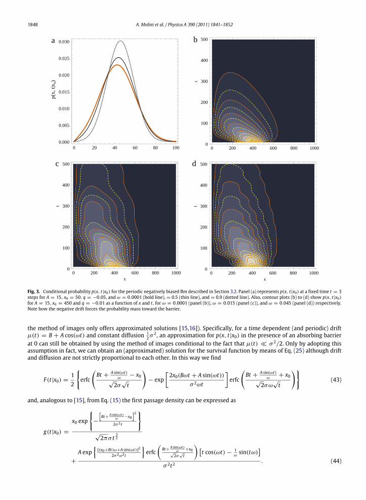
where, again, the absorption at the barrier represents a recurrent (q < 0) or a transient (q > 0) state, as was observed forthe power-law drift and diffusion process in Section 3.1. The recurrent case is illustrated in Fig. 3 (b)–(d), where we reportthe time-position evolution of p(x, t|x0) as a function of increasing ω. From (39), given ω/ϑ(t) > 0, the expression for thesurvival function can be derived and takes the form

F(t|x0) = 12

�1 + erf

�qϑ(t)+4x0ω4√

ωϑ(t)

�+ exp (−qx0) erfc

�qϑ(t)−4x0ω4√

ωϑ(t)

�− 2 exp (−qx0)

�, (40)

which, given the equality erfc(−x) = 2 − erfc(x), can be alternatively expressed as

F(t|x0) = Φ

�qϑ(t) + 4x0ω2√2ωϑ(t)

�− exp (−qx0) Φ

�qϑ(t) − 4x0ω2√2ωϑ(t)

�. (41)

The first passage time density g(t|x0) is given by

g(t|x0) = 4A2x0√π

ω3/2 cos(ωt)2

ϑ(t)3/2 exp

�− (qϑ(t) + 4x0ω)2

16ωϑ(t)

�. (42)

The method of images can also be applied to the solution of different forms of periodic drivers, such as the caseµ(t) = q(B+A cos(ωt)) and σ (t) = √

2(B + A cos(ωt)), with (B+A cos(ωt)) > 0. In this last case, the drift term is the sameas the one usually investigated in neuron dynamics by simple integrate-and-firemodels displaying stochastic resonance (seefor example the neuron dynamics case in [15,16]. In those models, the diffusion is usually constant so that the condition inEq. (20) is not satisfied. Thus, it is often implied that µ(t) � σ 2/2 approximately resembles a time dependent diffusionwith drift identically vanishing or that B � A (approximating the simpler constant drift and diffusion case). In these cases,

1848 A. Molini et al. / Physica A 390 (2011) 1841–1852

0.000

0.005

0.010

0.015

0.020

0.025

0.030

p(x,

t|x 0

)

0 20 40 60 80 100 00

100

200

300

400

500

200 400 600 800 1000

t

00

100

200

300

400

500

200 400 600 800 1000

t

00

100

200

300

400

500

200 400 600 800 1000

t

x x

a b

c d

Fig. 3. Conditional probability p(x, t|x0) for the periodic negatively biased Bm described in Section 3.2. Panel (a) represents p(x, t|x0) at a fixed time t = 3steps for A = 15, x0 = 50, q = −0.05, and ω = 0.0001 (bold line), = 0.5 (thin line), and = 0.9 (dotted line). Also, contour plots (b) to (d) show p(x, t|x0)for A = 15, x0 = 450 and q = −0.01 as a function of x and t , for ω = 0.0001 (panel (b)), ω = 0.015 (panel (c)), and ω = 0.045 (panel (d)) respectively.Note how the negative drift forces the probability mass toward the barrier.

the method of images only offers approximated solutions [15,16]). Specifically, for a time dependent (and periodic) driftµ(t) = B + A cos(ωt) and constant diffusion 1

2σ2, an approximation for p(x, t|x0) in the presence of an absorbing barrier

at 0 can still be obtained by using the method of images conditional to the fact that µ(t) � σ 2/2. Only by adopting thisassumption in fact, we can obtain an (approximated) solution for the survival function by means of Eq. (25) although driftand diffusion are not strictly proportional to each other. In this way we find

F(t|x0) = 12

�

erfc

�Bt + A sin(ωt)

ω− x0√

2σ√t

�

− exp�2x0(Bωt + A sin(ωt))

σ 2ωt

�erfc

�Bt + A sin(ωt)

ω+ x0√

2σω√t

��

(43)

and, analogous to [15], from Eq. (15) the first passage density can be expressed as

g(t|x0) =x0 exp

�

−�Bt+ A sin(ωt)

ω −x0�2

2σ 2t

�

√2πσ t

32

+A exp

�[(x0+Bt)ω+A sin(ωt)]2

2σ 2ω2t

�erfc

�Bt+ A sin(ωt)

ω +x0√2σ

√t

� �t cos(ωt) − 1

ωsin(tω)

�

σ 2t2. (44)

A. Molini et al. / Physica A 390 (2011) 1841–1852 1849

0.001

0.002

0.003

0.004

0.005

200 400 600 800 1000

200 400 600 800 1000

g(t|x

0)

0.010

0.002

0.004

0.006

0.008

t

0.001

0.002

0.003

0.004

0.005

0.006

200 400 600 800 1000

200 400 600 800 1000

0.010

0.002

0.004

0.006

0.008

t

a b

c d

g(t|x

0)

Fig. 4. First passage densities g(t|x0) (bold black line, Eq. (44)), and g̃(t|x0) (red dotted line, Eq. (45)), respectively for (a) µ = 0.065, σ = 0.5, x0 = 25,A = 0.032 and ω = 0.016; (b) µ = 0.065, σ = 0.35, x0 = 15.5, A = 0.025 and ω = 0.04; (c) µ = 0.065, σ = 0.2, x0 = 25, A = 0.03 and ω = 0.07,and (d) µ = 0.065, σ = 0.2, x0 = 25, A = 0.03 and ω = 0.15. The discrepancy between g̃(t|x0) and g(t|x0) clearly signifies the failure of the method ofimages for problems with time-dependent Péclet numbers. (For interpretation of the references to colour in this figure legend, the reader is referred to theweb version of this article.)

The approximated nature of the solution is evidenced by the fact that, the image source intensity is no longer constant intime, so that by evaluating the probability current in 0 we obtain

g̃(t|x0) = x0√2πσ t3/2

exp�− [ω(Bt − x0) + A sin(ωt)]2

2ω2σ 2t

�, (45)

which is different from (44). In any case, the first passage time pdf in Eq. (44) is in good agreement with the numericalsimulations in [15,16]. Also, when A → 0 both the (44) and the (45) tend to the first passage time pdf for a simple biasedBm.

As highlighted in Fig. 4, when the magnitude of µ(t) becomes significant, the two pdfs diverge due to the losses ofprobability density at the barrier (Eq. (45)). For this reason, the method of images cannot be considered a general approachto solving problems described by Eq. (3) with a time-dependent Péclet number.

4. A case study: snowmelt dynamics

Snowmelt represents one of the paramount sources of freshwater for many regions of the world, and is sensitive toboth temperature and precipitation fluctuations [33–38]. Snow dynamics is characterized by an accumulation phase duringwhich snow water equivalent (i.e. the amount of liquid water potentially available by totally and instantaneously meltingthe entire snowpack) increases until a seasonal maximum h0 is reached, followed by a depletion phase in which the snowmantle gradually decays (and releases the stored water content) due to the increasing air temperature. Such a dynamicsis complex and its general description requires numerous physical parameters that are rarely measured or available. Inthis section, we focus on a stochastic model describing the total water equivalent from both snow and rainfall during themelting season, as forced/fed by both precipitation (moving from the solid to the liquid precipitation regime) and increasingair temperature.

Due to the simplified nature of our stochastic model, we will consider the total potential water availability (interms of water equivalent) as the key variable, thus neglecting any further effects connected with snow percolation andmetamorphism [39]. Snowfalls are here assumed to become more sporadic progressing into the warm season and thepredominant controls over fresh water availability during the melting period are increasing air temperature and liquidprecipitation. Accordingly, the melting phase is described by a power-law time dependent drift directed towards the totaldepletion of the snow mantle and by a power-law diffusion whose positive and negative excursions represent respectivelyprecipitation events and pure melting periods. The melting process is often described by a linear function of time by using

1850 A. Molini et al. / Physica A 390 (2011) 1841–1852

00

0

2

4

6

0

0

0.02

0.04

0.06

50 100

0.2

0.2

0.4

0.4

0.6

0.6

0.8

0.8

1

t[days]

0 50 100

t[days] t[days]

h (s

imul

ated

) [m

]g(

t | h

0)

h[m]

p(h,

t | h

0)

100

101 102

10-5

F(t |

h0)

a b

c d

Fig. 5. Sample trajectories of specificwater equivalent from elevated regions during themelting season (a), and analytical results for the coupled stochasticmelting-precipitation process of Eq. (46) (panels (b) to (d)). Numerical results were obtained by simulating Eq. (46) by means of an Euler algorithm withstep 10−2 days. Panel (a) shows a few sample trajectories of the process together with the curve of maximum values (upper curve) and minimum values(lower curve) over an ensemble of 10000 simulations, for α = 0.25 and k = 0.24 mm2/daysα . Analytical results for the conditional probability p(h, t|h0)at different instants, the first passage time density g(t|h0), and the survival function F(t|h0), are also shown in panels (b)–(d).

the so called ‘‘degree-day’’ approach with time-varying melting-rate coefficients [39]. Considering that temperature variesseasonally and increases during the melting season, a power-law form for drift and diffusion during the spring season, stillrepresents a parametrically-parsimonious and effective approximation of the basic driver of the process.

Under these assumptions, the dynamics of the total water equivalent depth for unit of area h — i.e. the amount offresh water potentially available from both snow accumulation and rainfall [40] — at a given point in space can be canbe reasonably described by the Langevin equation

dh = −qktαdt +

√2ktαdW (t) (46)

where k (with dimension L2/Tα+1) represents the accumulation/ablation rate. Note that here h includes both the rainfall and

snowmelt contributions. Also, we hypothesize that both the drift and the diffusion scale with the same exponent α. This isa reasonable assumption given that variability of the process is expected to increase proceeding into the warm season.The initial condition is given by the snow water equivalent (SWE) h0, accumulated during the cold season. The survivalprobability F(t|h0) for a given initial SWE and the first passage time density g(t|h0) can be respectively calculated from (34)and (35). Fig. 5 shows few sample trajectories of the process (panel (a)) obtained by the numerical simulation of Eq. (46) bymeans of a forward Euler algorithmwith a time step of 10−2 days. The conditional probability p(h, t|h0) at different instants,the first passage time density g(t|h0), and the survival function F(t|h0), for the case α = 0.25 and k = 0.24 mm2/daysα arealso shown in panels (b)–(d). Here,we calibrated the parameters to obtain themode of the first passage time at about 40 daysafter reaching the maximum SWE of the season h0. The first passage time statistics presented offer important clues aboutthe timing between melting and summer fresh-water availability under different climatic scenarios (consider for examplethe FPT pdf in Fig. 5(c)).

A. Molini et al. / Physica A 390 (2011) 1841–1852 1851

5. Conclusions

The first passage time properties of Brownian motion with purely time-dependent drift and diffusion coefficientssubjected to an absorbing barrier were investigated. These processes can be used to mimic a variety of environmental andgeophysical phenomena, representing the availability of a resource and its dynamics in time (e.g. the ablationphase of a snowmass accumulated during the winter period and forced by temperature and precipitation). Survival functions and pdfs forthe first passage times at the barrier were derived for power-law and periodic forcing time-dependent drift and diffusionterms for the associated Fokker–Planck equation using the method of images. The general properties and limitations ofthis method were also reviewed, with reference to previous results obtained in the field of neural sciences and stochasticresonance. Particularly, we discussed how the applicability of the method of images to a Bmwith time-dependent drift anddiffusion is limited to the case of a process with constant Péclet number, i.e. with a time-independent ratio of drift anddiffusion.

Where the time-dependence is of the power-law type, the derived first passage time density and survival functions sharemany analogies with the statistics of inter-arrival times between intermittent events when the considered system displayssporadic randomness. In the case of a periodic time-dependence, first passage time statistics appear to be modulated by thefrequency of the forcing. The periodic forcing case has been also used to show the approximate nature of solutions obtainedby the method of images, when time-dependent drift and diffusion terms are not linearly related. We finally show howa Bm with power-law decaying drift and diffusion can be used to describe the warm season dynamics of the total waterequivalent in mountainous regions.

Acknowledgements

This study was supported, in part, by the National Science Foundation (NSF EAR 1063717, NSF-EAR 0628342, NSF-EAR0635787 and NSF-ATM-0724088), and the Bi-national Agricultural Research and Development (BARD) Fund (IS-3861-96).We wish to thank Adi Bulsara for the helpful suggestions. We also thank Demetris Koutsoyiannis and the other threeanonymous reviewers for their helpful suggestions.

References

[1] J. Ehleringer, T. Cerling, B. Helliker, C-4 photosynthesis, atmospheric CO2 and climate, Oecologia 112 (1997) 285–299.[2] T. McClanahan, J. Maina, Response of coral assemblages to the interaction between natural temperature variation and rare warm-water events,

Ecosystems 6 (2003) 551–563.[3] C. Rosenzweig, M. Parry, Potential impact of climate-change on world food supply, Nature 367 (1994) 133–138.[4] D. Marks, J. Kimball, D. Tingey, T. Link, The sensitivity of snowmelt processes to climate conditions and forest cover during rain-on-snow: a case study

of the 1996 Pacific Northwest flood, Hydrol. Process. 12 (1998) 1569–1587.[5] A. Hamlet, D. Lettenmaier, Effects of climate change on hydrology and water resources in the Columbia river basin, J. Am. Water Resour. Assoc. 35

(1999) 1597–1623.[6] C. Barranguet, J. Kromkamp, J. Peene, Factors controlling primary production and photosynthetic characteristics of intertidalmicrophytobenthos, Mar.

Ecol. Prog. Ser. 173 (1998) 117–126.[7] M. Bertness, G. Leonard, The role of positive interactions in communities: lessons from intertidal habitats, Ecology 78 (1997) 1976–1989.[8] H. Charles, J.S. Dukes, Effects of warming and altered precipitation on plant and nutrient dynamics of a new england salt marsh, Ecol. Appl. 19 (2009)

1758–1773.[9] M. Pascual, M. Bouma, A. Dobson, Cholera and climate: revisiting the quantitative evidence, Microbes Infect. 4 (2002) 237–245.

[10] J. Patz, D. Campbell-Lendrum, T. Holloway, J. Foley, Impact of regional climate change on human health, Nature 438 (2005) 310–317.[11] C. Adami, Self-organized criticality in living systems, Phys. Lett. A 203 (1995) 29–32.[12] P. Bak, M. Paczuski, Complexity, contingency, and criticality, Proc. Natl. Acad. Sci. USA 92 (1995) 6689–6696.[13] H.J. Jensen, Self-Organized Criticality: Emergent Complex Behavior in Physical and Biological Systems, in: Cambridge Lecture Notes in Physics,

Cambridge University Press, Cambridge, UK, New York, NY, USA, 1998.[14] S. Redner, A Guide to First Passage Processes, Cambridge University Press, Cambridge, UK, 2001.[15] A.R. Bulsara, S.B. Lowen, C.D. Rees, Cooperative behavior in the periodically modulatedWiener process: noise-induced complexity in a model neuron,

Phys. Rev. E 49 (1994) 4989–5000.[16] A.R. Bulsara, S.B. Lowen, C.D. Rees, Reply to coherent stochastic resonance in the presence of a field, Phys. Rev. E 52 (1995) 5712–5713.[17] L. Gammaitoni, P. Hanggi, P. Jung, F. Marchesoni, Stochastic resonance, Rev. Modern Phys. 70 (1998) 223–287.[18] M. McDonnell, N. Stocks, C. Pearce, D. Abbott, Stochastic Resonance: From Suprathreshold Stochastic Resonance to Stochastic Signal Quantization,

Cambridge University Press, Cambridge, UK, 2008.[19] W. Feller, An Introduction to Probability Theory and its Applications, 3rd ed., vol. 2, Wiley, 1971.[20] C. Kim, P. Talkner, E.K. Lee, P. Haenggi, Rate description of Fokker–Planck processes with time-periodic parameters, Chem. Phys. 370 (2010) 277–289.[21] P. Jung, Periodically driven stochastic-systems, Phys. Rep. 234 (1993) 175–295.[22] P. Talkner, L. Machura, M. Schindler, P. Hanggi, J. Luczka, Statistics of transition times, phase diffusion and synchronization in periodically driven

bistable systems, New J. Phys. (2005) 7.[23] M. Schindler, P. Talkner, P. Hanggi, Escape rates in periodically driven Markov processes, Physica A 351 (2005) 40–50.[24] A. Polyanin, Handbook of Linear Partial Differential Equations for Engineers and Scientists, Chapman and Hall/CRC, New York, NY, USA, 2002.[25] D.R. Cox, H.D. Miller, The Theory of Stochastic Processes, Chapman & Hall, CRC, Boca Raton, Florida, USA, 1965.[26] H. Daniels, Sequential tests constructed from images, Ann. Statist. 10 (1982) 394–400.[27] V. Lo, G. Roberts, H. Daniels, Sequential tests constructed from images, Bernoulli 8 (2002) 53–80.[28] M. Abramowitz, I.A. Stegun, Handbook of Mathematical Functions with Formulas, Graphs, and Mathematical Tables, ninth dover printing, tenth GPO

printing ed., Dover, New York, 1964.[29] N. Johnson, S. Kotz, N. Balakrishnan, Continuous Univariate Distributions, vol. 1, Wiley and Sons, New York, USA, 1994.[30] P. Gaspard, X. Wang, Sporadicity—between periodic and chaotic dynamical behaviors, Proc. Natl. Acad. Sci. USA 85 (1988) 4591–4595.[31] A. Molini, G.G. Katul, A. Porporato, Revisiting rainfall clustering and intermittency across different climatic regimes, Water Resour. Res. 45 (2009).[32] J.R. Rigby, A. Porporato, Precipitation, dynamical intermittency, and sporadic randomness, Adv. Water Resour. 33 (2010) 923–932.

1852 A. Molini et al. / Physica A 390 (2011) 1841–1852

[33] T. Barnett, R. Malone, W. Pennell, D. Stammer, B. Semtner, W.Washington, The effects of climate change on water resources in the west: introductionand overview, Clim. Change 62 (2004) 1–11.

[34] T.P. Barnett, J.C. Adam, D.P. Lettenmaier, Potential impacts of a warming climate on water availability in snow-dominated regions, Nature 438 (2005)303–309.

[35] T.P. Barnett, D.W. Pierce, Sustainable water deliveries from the Colorado river in a changing climate, Proc. Natl. Acad. Sci. USA 106 (2009) 7334–7338.[36] P. Perona, P. D’Odorico, A. Porporato, L. Ridolfi, Reconstructing the temporal dynamics of snow cover from observations, Geophys. Res. Lett. 28 (2001)

2975–2978.[37] N.C. Pepin, J.D. Lundquist, Temperature trends at high elevations: patterns across the globe, Geophys. Res. Lett. 35 (2008).[38] Q.L. You, S.C. Kang, N. Pepin, W.A. Flugel, Y.P. Yan, H. Behrawan, J. Huang, Relationship between temperature trend magnitude, elevation and mean

temperature in the tibetan plateau from homogenized surface stations and reanalysis data, Glob. Planet. Change 71 (2010) 124–133.[39] D. De Walle, A. Rango, Principles of Snow Hydrology, Cambridge University Press, Cambridge, UK, 2008.[40] R.L. Bras, Hydrology: An Introduction to Hydrological Science, Addison-Wesley, Reading, MA, 1990.