First-Passage-Time Prototypes for Precipitation Statistics

First-Passage-Time Prototypes for Precipitation Statistics

SAMUEL N. STECHMANN

Department of Mathematics, and Department of Atmospheric and Oceanic Sciences, University of

Wisconsin—Madison, Madison, Wisconsin

J. DAVID NEELIN

Department of Atmospheric and Oceanic Sciences, University of California, Los Angeles, Los Angeles, California

(Manuscript received 29 August 2013, in final form 27 December 2013)

ABSTRACT

Prototype models are presented for time series statistics of precipitation and column water vapor. In these

models, precipitation events begin when the water vapor reaches a threshold value and end when it reaches

a slightly lower threshold value, asmotivated by recent observational andmodeling studies. Using a stochastic

forcing to parameterize moisture sources and sinks, this dynamics of reaching a threshold is a first-passage-

time problem that can be solved analytically. Exact statistics are presented for precipitation event sizes and

durations, for which the model predicts a probability density function (pdf) with a power law with exponent

23/2. The range of power-law scaling extends from a characteristic small-event size to a characteristic large-

event size, both of which are given explicitly in terms of the precipitation rate and water vapor variability.

Outside this range, exponential scaling of event-size probability is shown. Furthermore, other statistics can be

computed analytically, including cloud fraction, the pdf of water vapor, and the conditional mean and vari-

ance of precipitation (conditioned on thewater vapor value). These statistics are comparedwith observational

data for the transition to strong convection; the stochastic prototype captures a set of properties originally

analyzed by analogy to critical phenomena. In a second prototype model, precipitation is further partitioned

into deep convective and stratiform episodes. Additional exact statistics are presented, including stratiform

rain fraction and cloud fractions, that suggest that even very simple temporal transition rules (for stratiform

rain continuing after convective rain) can capture aspects of the role of stratiform precipitation in observed

precipitation statistics.

1. Introduction

Cloud and precipitation processes are initiated at

a natural threshold when water vapor reaches a satura-

tion value. In addition, clouds and precipitation involve

turbulent variability that can often be modeled sto-

chastically. Taken together, a stochastic process with a

threshold is a first-passage-time problem (Redner 2001;

Gardiner 2004). The main purpose of this paper is to

present first-passage-time prototype models for precip-

itation and water vapor statistics. A key aspect of the

models here is that they are exactly solvable.

Thresholds arise in various ways in conjunction with

clouds and precipitation. On small scales, for instance,

the Clausius–Clapeyron equation provides a threshold

for saturation. In large-scale models, convective pa-

rameterizations include a threshold for convective on-

set, such as the one used by the Betts–Miller adjustment

scheme (Betts 1986).

In recent studies, a threshold has been identified em-

pirically for the transition to strong convection as a

function of bulk environmental variables such as column

water vapor (CWV) and tropospheric vertical-average

temperature, on scales of O(20) km or larger, as sum-

marized in Fig. 1a. When CWV is below the threshold,

mean precipitation is small, and when CWV exceeds the

threshold, mean precipitation increases rapidly. Peters

and Neelin (2006) noted that in certain respects the

threshold resembles a critical point in statistical physics

terminology, and used this well-studied prototype for

statistics of ensembles of interacting elements near

a transition, along with related self-organized criticality

prototypes (Christensen and Moloney 2005), to suggest

Corresponding author address: Samuel N. Stechmann, University

of Wisconsin—Madison, Department of Mathematics, 480 Lincoln

Dr., Madison, WI 53706.

E-mail: [email protected]

SEPTEMBER 2014 S TECHMANN AND NEEL IN 3269

DOI: 10.1175/JAS-D-13-0268.1

� 2014 American Meteorological Society

mailto:[email protected]

a set of properties to examine in observations. These

include power-law ranges in spatial and temporal cor-

relation and in event-size distributions (Peters et al.

2001, 2010); see Fig. 1b. Furthermore, the ‘‘critical

point’’ is similar to the equilibrium state envisioned by

the theory of convective quasi equilibrium (Arakawa

and Schubert 1974), in that it is associated with the onset

of conditional instability (Holloway and Neelin 2009),

and the resulting dissipation of entraining convective

available potential energy above critical results in prob-

ability density functions (pdfs) of CWV for precipitating

points that peak just below the critical point (Figs. 1a,c).

Such statistics can potentially serve to constrain or im-

prove convective parameterizations in general circulation

models (GCMs) (Neelin et al. 2008). For this, it can be

useful to have more precise prototype models that relate

directly to the equations of atmospheric models and that

can explicitly examine how such pdfs arise, including

contributions of large-scale and subgrid-scale processes.

To this end, Stechmann and Neelin (2011, hereafter

SN11) designed a simple stochastic model for the evo-

lution of CWV and precipitation. In that model,

a prognostic equation for CWVwas driven by stochastic

forcing representing large-scale moisture convergence

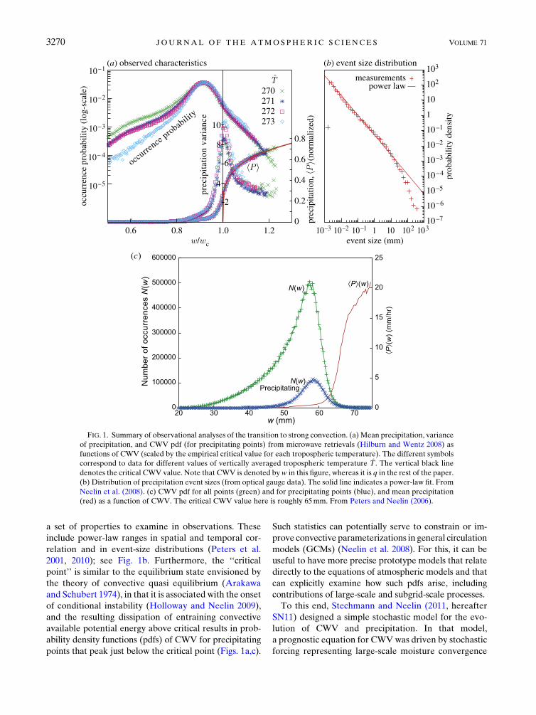
FIG. 1. Summary of observational analyses of the transition to strong convection. (a) Mean precipitation, variance

of precipitation, and CWV pdf (for precipitating points) from microwave retrievals (Hilburn and Wentz 2008) as

functions of CWV (scaled by the empirical critical value for each tropospheric temperature). The different symbols

correspond to data for different values of vertically averaged tropospheric temperature T̂. The vertical black line

denotes the critical CWV value. Note that CWV is denoted byw in this figure, whereas it is q in the rest of the paper.

(b) Distribution of precipitation event sizes (from optical gauge data). The solid line indicates a power-law fit. From

Neelin et al. (2008). (c) CWV pdf for all points (green) and for precipitating points (blue), and mean precipitation

(red) as a function of CWV. The critical CWV value here is roughly 65mm. From Peters and Neelin (2006).

3270 JOURNAL OF THE ATMOSPHER IC SC IENCES VOLUME 71

and (in the precipitating state) a stochastic contribution

to precipitation, and furthermore a stochastic threshold

was used: when CWV reaches the critical value, precip-

itation is allowed to begin with some probability, but it

does not necessarily begin precisely at the critical value.

This stochastic threshold was motivated by the statistical

nature of the observed threshold (Neelin et al. 2009) and

by earlier use of stochastic jump processes for parame-

terizing convective transitions (Majda and Khouider

2002;Majda and Stechmann 2008).At the critical value of

CWV, the model of SN11 reproduced the transition in

mean precipitation and the peak in precipitation vari-

ance. The mean and variance are also captured by the

model of Muller et al. (2009), which uses a simpler setup

that neglects evolution in time but does consider sto-

chastic effects in the presence of an onset boundary. In

the time-evolving model of SN11, the additional statistics

in Fig. 1 were also reproduced, including the pdf of CWV

and the distribution of precipitation event sizes.

To better understand some of the processes that are

captured numerically in SN11, themodel presented here

uses a number of simplifications including a fixed

threshold rather than a stochastic threshold. While this

simplification may come at the expense of some realism,

it allows analytical solutions to be found. Consequently,

errors from statistical sampling of Monte Carlo realiza-

tions are absent, and exact statistics can be presented

unambiguously. Furthermore, interesting relationships

are revealed by comparing formulas for different sta-

tistics. For example, the same characteristic CWV value,

P*/D21, will appear as an important element of both the

precipitation-event–size distribution and the CWV pdf;

and, in addition, this characteristic value is related to

a precipitation rate P* and a water vapor forcing vari-

anceD21. Through these statistical relationships and this

type of insight, the present paper is aimed at two ques-

tions: What is the simplest prototype model for pre-

cipitation and water vapor statistics? What does the

model reveal about the underlying physical processes?

Among the various types of rainfall models in exis-

tence, the models presented here are most similar to

those that use renewal processes (Cox 1962; Green 1964;

Roldán and Woolhiser 1982; Foufoula-Georgiou and

Lettenmaier 1987; Schmitt et al. 1998; Bernardara et al.

2007), although many of these previous models apply to

daily precipitation, whereas the present focus includes

subdaily time scales. A distinguishing feature of the

present paper is that the renewal process for precip-

itation events is not an isolated process; rather, it arises

from the dynamics of the water vapor.

Furthermore, regarding precipitation–water vapor

relationships, the models here are aimed at the suite of

observational analyses (Peters and Neelin 2006; Neelin

et al. 2009) summarized above. In providing tractable

solutions that imitate this set of properties in a first-

passage setting, it should be possible to make more

precise statements about the relationship of the con-

vective transition to properties of self-organized criti-

cality (Peters and Neelin 2006; Christensen and Moloney

2005), which can sometimes be described in terms of first-

passage problems (Redner 2001; Sornette 2004). Further

studies of these topics have been undertaken with cloud-

resolvingmodels (Yano et al. 2012; S.K.Krueger andA.K.

Kochanski 2013, personal communication). In the present

study, by reproducing a suite of the observed statistics in

an exactly solvable model, the aim is to better understand

the underlying physical processes. An aspect of particular

interest is the distribution of sizes of precipitation events

(Peters et al. 2001, 2010). As shown in Fig. 1b, the event-

size distribution follows a power law over a wide range

of event sizes. As a further surprise, similar event-size dis-

tributions are seen at many locations around the world,

despite major differences in their local climates. This uni-

versality suggests that, even across awide range of climates,

some common aspects exist in disparate classes of pre-

cipitation events.

The partitioning of precipitation into deep convective

and stratiform components has long been investigated

(Cheng and Houze 1979; Steiner et al. 1995; Short et al.

1997; Rickenbach and Rutledge 1998; Schumacher and

Houze 2003; Yuter et al. 2005). The importance of this

partitioning is multifaceted; as one example, these

components have different profiles of vertical heating,

which has important consequences for atmospheric dy-

namics (Houze 1989; Mapes 1993, 2000; Schumacher

et al. 2004; Khouider andMajda 2006; Tulich et al. 2007;

Khouider and Majda 2008; Majda and Stechmann 2009;

Stechmann and Majda 2009). One of the models in the

present paper will include these two components—

deep convective and stratiform—and will have exactly

solvable statistics for stratiform rain fraction and con-

vective rain fraction. This permits examination in the

temporal domain of the role transitions to and from

stratiform precipitation can play near the critical point

of Fig. 1.

In short, the aim here is to ask what aspects of the

observed statistics can be imitated in a model that only

contains time evolution of column-integrated water va-

por and simple onset thresholds that switch among

precipitation states, including a dependence on the di-

rection of the threshold is crossed. In the two-state

model, there is a nonprecipitating state in which an

evaporation-like source term creates an upward drift

in moisture toward the precipitation onset threshold,

and a precipitating state in which precipitation creates

a drift toward lower moisture, with the cessation of


precipitation occurring at a slightly smaller value than

the onset threshold. In both states, moisture con-

vergence and/or divergence by fluctuating large-scale

dynamics is represented by a stochastic term. In the three-

state model, the consequences of distinguishing between

a deep convective and a stratiform precipitating state are

analyzed, with the stratiform state occurring within a cer-

tain range asmoisture decreases from the deep convective

state. In observations or three-dimensional models, there

can be spatial interactions that potentially affect evolution

in realistic states corresponding to these. The analysis here

indicates the statistics for a fairly extensive set of phe-

nomenon can be at least qualitatively captured with sim-

ple time-evolution rules.

A complementary relationship may be noted to

advection–condensationmodels or time-of-last-saturation

analysis (e.g., Pierrehumbert 1998; Galewsky et al. 2005;

O’Gorman and Schneider 2006; Pierrehumbert et al.

2007; Sukhatme and Young 2011; O’Gorman et al.

2011). These examine the pdf or other statistics of water

vapor—for instance, under stochastic advection on an

isentropic surface—taking the last saturation as a

boundary at which the humidity is set to saturation.

Here, evolution is similarly driven by a stochastic rep-

resentation of advection effects, but the threshold cor-

responds to the onset of conditional instability in the

column, rather than to saturation, and thus water vapor

can continue to exhibit nontrivial dynamics in the in-

terval above the threshold. Quantities of interest thus

include statistics such as the pdfs of precipitating points

on both sides of the threshold and event-size distri-

butions. Evolution on the nonprecipitating side is

analogous to the advection–condensation models. For

instance, Pierrehumbert et al. (2007) note a scaling range

for the distribution of intervals between encounters with

the saturation boundary that corresponds to that found

for dry spells in the present model.

The paper is organized as follows. In sections 2–4,

a two-state model is presented for convective onset and

shutdown. After the model description in section 2, the

distributions of event sizes and durations are presented

in section 3, and further statistics are presented in sec-

tion 4. In section 5, a three-state model is presented that

partitions precipitation events into deep convective and

stratiform episodes. Discussion and conclusions follow

in sections 6 and 7, and the appendixes describe some of

the calculations.

2. Two-state model for convective onset

In this section a two-state model is presented for onset

and shutdown of convective events. The two states are

wet spells and dry spells, where the wet spells are times

of precipitation. This is the simpler of the two prototype

models considered here.

The model involves the stochastic evolution of the

water vapor q(t) for a single atmospheric column. The

dynamics of q(t) depends on whether the column is

nonprecipitating or precipitating:

dq

dt5E*1D0

_j if nonprecipitating, (1)

dq

dt52P*1D1

_j if precipitating. (2)

Here _j is Gaussian white noise, E* is a constant

‘‘evaporation’’ rate, P* is a constant precipitation rate,

and D0 and D1 are constants that measure the variance

of water vapor forcing. While E* is referred to as an

evaporation rate for simplicity, it represents a mean

moisture source due to all relevant processes, such as

surface fluxes and moisture advection. Similarly, P* is

the net moisture sink in the precipitating state and so

strictly speaking would be precipitation minus evapo-

ration and mean moisture convergence. For simplicity,

we discuss it as a precipitation rate here. While it is

a crude simplification to treat these moisture sources

and sinks as constants, it will allow analytic solutions,

and it can be evaluated a posteriori by comparing the

statistics from the model and observations.

The values of the model parameters are listed in

Table 1. At the moment, the parameter values are

chosen based on a comparison between observed sta-

tistics and exact theoretical statistics, the latter of which

is presented below. In the future, it would be interesting

to directly estimate these parameters from observations

or model data.

Whether the column is precipitating or nonprecipitating

is determined by two thresholds, as illustrated in Fig. 2. If

the column is nonprecipitating and q(t) increases to the

critical value qc, then precipitation begins. The dynamics

of q(t) switches from (1) to (2). The column remains in

the precipitating state until q(t) decreases to a different,

lower threshold qnp. Upon reaching qnp, the column is

nonprecipitating again, and the cycle repeats:

TABLE 1. Parameters for the two-state model for convective onset.

Symbol Description Value

P* Precipitation rate 3mmh21

E* Evaporation rate 0.4mmh21

D21 Forcing variance (s 5 1) 64mm2h21

D20 Forcing variance (s 5 0) 8mm2h21

qc Critical CWV 65mm

qnp Low-threshold CWV 62mm

b qc 2 qnp 3mm


dq

dt5E*1D0

_j until q5qc ,

dq

dt52P*1D1

_j untilq5 qnp ,

dq

dt5E*1D0

_j until q5 qc ,

dq

dt52P*1D1

_j untilq5 qnp ,

..

.(3)

To keep track of the state of the column as non-

precipitating or precipitating, an indicator variable s(t)

is assigned the value of 0 or 1, respectively:

nonprecipitating s(t)5 0 untilq5 qc ,

precipitating s(t)5 1 untilq5 qnp ,

nonprecipitating s(t)5 0 untilq5 qc ,

precipitating s(t)5 1 untilq5 qnp ,

..

.(4)

Notice that knowledge of q(t) alone is not always

sufficient to determine whether the column is precipi-

tating or nonprecipitating. If CWV is in the intermediate

range qnp , q , qc between the two thresholds, the

column could be either precipitating or nonprecipitating,

and it is the variable s(t) that records the ‘‘memory’’ of

whether the column is precipitating.

Also notice that it is possible for q(t) to increase be-

yond qc during a precipitation event, despite P*. This

can happen if the stochastic source–sink term D1_j,

which can be either positive or negative, over-

compensates for the loss due P*; see Fig. 2 at roughly

time t 5 10 h for an example. In nature, such a strong

moisture source would typically be due to moisture

convergence that is crudely represented here by D1_j.

SN11 identified such excursions of q(t) . qc with the

longest-lasting precipitation events in their model. They

also identified a portion of the source–sink termwith the

precipitation process itself; for the sake of analytic so-

lutions in certain precipitation statistics this is omitted

here (although it is a straightforward extension for many

aspects of the model).

One of the main differences between this model and

the model of SN11 is that here precipitation events al-

ways start immediately when q(t) increases to qc and

always end immediately when q(t) decreases to qnp. In

contrast, in the model of SN11, the start and end of

precipitation events were governed by a stochastic jump

process. The model in (3) can be viewed as a limiting

case of themodel of SN11: in the limit that the stochastic

jump rates become infinite, the system transitions im-

mediately when the threshold qc or qnp is reached.

A second difference from themodel of SN11 is thatP*and D1 are constants in (1) and (2). In contrast, in the

model of SN11, P*(q) and D1(q) were taken to be q-

dependent functions as a way to allow both intense and

moderate stages of a precipitation event, to represent

deep convective and stratiform rainfall, respectively.

Later, in section 5, a three-state model is presented that

includes both deep convective and stratiform precipita-

tion. As a simpler prototype, the two-state model in (1)

and (2) is presented here first, and it will already display

many of the main desired features. Its precipitation rate

of P* 5 3mmh21 is meant to be an average or typical

precipitation rate during precipitation events (i.e., much

higher than the long-term average precipitation rate),

characteristic of neither deep convection nor stratiform

precipitation exclusively, yet closer to characteristics of

stratiform precipitation (Nesbitt et al. 2006).

FIG. 2. Sample time series of (top) CWV q(t) and (bottom) precipitation indicator s(t) for 24 h. Dashed lines in the

top panel denote the threshold values qc and qnp. Water vapor is shown in black during dry spells and in gray during

wet spells.


We note that in SN11 numerical tests of correspond-

ing simplifications were carried out; these identified the

features maintained in this model as able to capture key

properties such as the power-law range in the event-size

distribution. These two simplifications allow exact ana-

lytic calculation of the precipitation and water vapor

statistics, as shown below.

3. Event-size pdf

An interesting statistic to consider is the event size,

which is defined as the total amount of precipitation

(mm) to fall during a precipitation event. Observational

analyses have shown that small events aremost probable

and that the distribution of event sizes decays like a

power law (Peters et al. 2001, 2010). See Fig. 1 for a re-

production of observational analysis.

For the two-state model, the event size is propor-

tional to the event duration, with proportionality con-

stant P*. Furthermore, the distributions can be found

analytically.

a. Analytic solution

The pdf pt1(t) of precipitation event durations comes

from solving the following first-passage-time problem:

given that q is initially at the critical value q 5 qc at the

start of the event, how long does it take q to decrease to

the low threshold qnp? The pdf for the event durations is

pt1(t)

5bffiffiffiffiffiffiffiffiffiffiffiffi2pD2

1

q exp

P*b

D21

!exp

2

b2

2D21t

!exp

2P2*t

2D21

!t23/2,

(5)

where b 5 qc 2 qnp. The derivation is given in the

appendix. Similarly, the distribution pt0(t) of dry-spell

durations is

pt0(t)

5bffiffiffiffiffiffiffiffiffiffiffiffi2pD2

0

q exp

E*b

D20

!exp

2

b2

2D20t

!exp

2E2*t

2D20

!t23/2 .

(6)

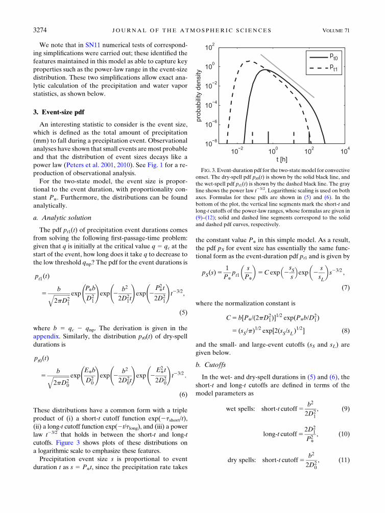
These distributions have a common form with a triple

product of (i) a short-t cutoff function exp(2tshort/t),

(ii) a long-t cutoff function exp(2t/tlong), and (iii) a power

law t23/2 that holds in between the short-t and long-t

cutoffs. Figure 3 shows plots of these distributions on

a logarithmic scale to emphasize these features.

Precipitation event size s is proportional to event

duration t as s 5 P*t, since the precipitation rate takes

the constant value P* in this simple model. As a result,

the pdf pS for event size has essentially the same func-

tional form as the event-duration pdf pt1 and is given by

pS(s)51

P*pt1

�s

P*

�5C exp

�2sSs

�exp

�2

s

sL

�s23/2 ,

(7)

where the normalization constant is

C5 b[P*/(2pD21)]

1/2 exp(P*b/D21)

5 (sS/p)1/2 exp[2(sS/sL)

1/2] (8)

and the small- and large-event cutoffs (sS and sL) are

given below.

b. Cutoffs

In the wet- and dry-spell durations in (5) and (6), the

short-t and long-t cutoffs are defined in terms of the

model parameters as

wet spells: short-t cutoff5b2

2D21

, (9)

long-t cutoff52D2

1

P2*

, (10)

dry spells: short-t cutoff5b2

2D20

, (11)

FIG. 3. Event-duration pdf for the two-statemodel for convective

onset. The dry-spell pdf pt0(t) is shown by the solid black line, and

the wet-spell pdf pt1(t) is shown by the dashed black line. The gray

line shows the power law t23/2. Logarithmic scaling is used on both

axes. Formulas for these pdfs are shown in (5) and (6). In the

bottom of the plot, the vertical line segments mark the short-t and

long-t cutoffs of the power-law ranges, whose formulas are given in

(9)–(12); solid and dashed line segments correspond to the solid

and dashed pdf curves, respectively.


long-t cutoff52D2

0

E2*

. (12)

For the parameters in Table 1, the power-law ranges are

then approximately given by

wet spells: 0:070, t, 14 h, (13)

dry spells: 0:56, t, 100 h. (14)

These cutoffs are indicated in Fig. 3 by the vertical line

segments in the bottom of the plot.

While the pdfs for wet- and dry-spell durations have

the same functional form, there is a clear asymmetry

between them: dry spells last longer than wet spells. A

simple quantification of this is in (13) and (14): the dry-

spell cutoffs are roughly 10 times longer than the wet-

spell cutoffs. This is roughly in agreement with the

observational analyses of Peters et al. (2010) and similar

to the analysis of daily data by Ratan and Venugopal

(2013). In the model here, the asymmetry can be related

to the model parameters. In (9)–(12), the exponential

cutoffs are related to characteristic time scales in terms

of the threshold separation, b5 qc 2 qnp; the variances,

D20 and D2

1; and the mean source and sink, E* and P*.

However, the ratios of the dry and wet cutoffs are in-

dependent of b. For the short-time cutoffs, the ratio is

D21/D

20; hence the cutoff for dry spells is longer because

the variance is smaller. Similarly, for the long-time cutoffs,

the ratio is (P2*/E

2*)/(D

21/D

20); hence the cutoff for dry

spells is longer because P2*/E

2* is even larger thanD2

1/D20.

Since pS is related to pt1 as shown in (7), its cutoff time

scales are related to characteristic water vapor values as

well. The relationship is a direct proportionality, withP*as the proportionality constant, which leads to

precipitation event sizes: small-s cutoff5b2P*2D2

1

, (15)

large-s cutoff52D2

1

P*, (16)

where the precipitation event size is measured in

millimeters. For the parameters in Table 1, the power-

law range is then approximately given by

precipitation event sizes: 0:21, s, 42mm. (17)

In (15) and (16), notice that the same characteristic

water vapor scale,D21/P*, appears in the expressions for

both the small-s and large-s cutoffs. Furthermore, as

shown below, this same characteristic scale appears in

the water vapor pdf as well.

To summarize, the pdfs of event duration and event

size have power-law scalingwith exponent23/2. However,

this scaling only holds over a finite range of durations and

sizes. Outside the power-law range, exponential scaling is

seen. In combination, these features characterize the ex-

treme events in this model. Not only does D21/P* appear

as the cutoff between power-law and exponential scaling,

but it also is the decay rate of the exponential scaling for

large events. This characteristic scale is a ratio of the

water vapor forcing variance and precipitation rate, and it

is the first of many statistical relationships that will be

suggested by the models.

c. Heuristic scaling

Why does the exponent 23/2 arise? And why is the

exponent independent of all model parameters? The

following heuristic argument addresses these questions

in relation to probability flux. In brief, probability den-

sity is proportional to t21/2, and probability flux inherits

an addition factor of t21 and is proportional to t23/2.

Consider the simpler case with P* 5 0 and with-

out thresholds. For this case, given q 5 0 ini-

tially, the probability density at a later time is

(2pD21t)

21/2 exp[2q2/(2D21t)], which is a Gaussian func-

tion with variance D21t. From this function, the probabil-

ity flux is obtained by Fick’s law and is proportional

to the derivative with respect to q—that is, it is pro-

portional to2(D21t)

23/2(q/ffiffiffiffiffiffi2p

p) exp[2q2/(2D2

1t)]. This is

the power lawwith exponent23/2.What is the connection

between the flux and the first-passage-time problem? By

definition, the flux indicates the probability that point q is

being passed at time t, and this is essentially the same as

the probability that a threshold is passed.

This heuristic argument indicates how the 23/2 expo-

nent arises and how it is related to probability flux. See

the appendix for a proper derivation including pre-

cipitation and a true threshold.

d. Mean and second moment of event-sizedistribution

The mean and second moments of the event-size

distribution are

hsi5b , (18)

hs2i5 bD2

1

P*1 hsi2 . (19)

The second moment diverges as expected as the large-

event-size cutoff goes to infinity—for example, for large

D21 or small P2

*. An interesting illustration of the use-

fulness of a physically based prototype is that the mean

remains finite in this limit. This is contrary to expectations


for a power law with exponent between 21 and 22,

such as the first-passage time in the limit as drift goes to

zero (Redner 2001, p. 84). Indeed, the mean duration

diverges as D21P

21* in this limit in the two-state model,

but the normalization for the event size includes the

drift rate P* in such a way that the mean event size

remains finite. To see directly from the equations why

this must occur, consider a time integral of (2) in the

precipitating regime. Over the duration of an event, the

dq/dt term integrates to2b, while the event size comes

fromÐ(2P*) dt. If one further takes an expectation

over all event sizes, theD1_j term drops out, yielding the

mean event size above.

The characteristics of the event-size distribution can

change in a way that is independent of the mean pre-

cipitation for the model, which is set by long-time av-

erage budget considerations and thus depends only on

P*E*/(P* 1 E*) (see section 4). If moisture conver-

gence variability, measured by D21, becomes large com-

pared to the P* and E* drift terms, a long power-law

range and large event-size variance can result even for

fixed mean rainfall.

As background for comparison to observations, the

two-state model ratio of first and second moments is

hs2ihsi 5

D21

P*1 b’

D21

P*} sL . (20)

This ratio for observational distributions in Peters et al.

(2010) was taken as an indicator of the large-s cutoff and

used to rescale event size at each of several instrument

locations. The two-state model confirms the usefulness

of this procedure while suggesting that (hs2i 2 hsi2)/hsimight be a slightly better measure.

In observations, the very-small-event-size portion of

the distribution is typically not reliably observed owing

to finite observation intervals and instrumentation error

at low rain rates. While in nature a small-event-size

cutoff might be affected by many processes including

temporal autocorrelation, the two-state model provides

a succinct case to examine potential impacts of not ob-

serving the cutoff regime. Consider integrals over an

interval of event sizes [s1, ‘). For the mean,ð‘s1

spS(s) ds5 b[12 �(sS, sL, s1)] , (21)

using (7), where � is small in both of the two most rele-

vant cases. First, �/ 0 for s1/ 0 (i.e., the full solution).

Furthermore, if we consider s1 to occur in the power-law

range as occurs in the data (i.e., s1/sS� 1), and that there

is a well distinguished power-law range [i.e., (sS/sL)1/2 �

1], we have

�’ 2p21/2(s1/sL)1/2 . (22)

Thus, if (sS/sL)1/2 � 1, � is small (i.e., the contribution to

the integral comes from the large-s end), and omission

of values less than s1 has little direct impact on the mean

or higher moments. The normalization is affected, since

forÐ ‘s1pS(s) ds, the dominant contribution is from close

to s1. However, a ratio such as (20) would not be.

e. Relation to observational data

We now turn to the question of how directly the

simple prototype can be compared to observations.

Peters et al. (2001) found a long power-law range in the

event-size distributions observed in radar data, with an

exponent of 21.36 while Neelin et al. (2008) estimated

an exponent of 21.3 from tropical data. Peters et al.

(2010) systematically examined event-size distributions

from Atmospheric Radiation Measurement Program

data. The power-law range for data from various loca-

tions is reasonably well fit by exponents of around21.2,

although some midlatitude cases yield individual esti-

mates from 21 to 21.4. Peters et al. (2010) also esti-

mated exponents of around 21.3 for power-law ranges

in dry period durations. For wet-spell-event durations,

the power-law range was much shorter; they suggested

an exponent of around 22, although examination of

their figures suggests that an exponent of 21.5 would

not be excluded. Andrade et al. (1998) show figures with

dry-spell exponents of around 21.8 and 21.9, noting

a wider range of exponents when examining other lo-

cations, and an exponent of about21.6 for rain duration

based on daily data. They discuss fits of both a second

power-law range and an exponential to the large-

duration cutoff.

In the two-state model as formulated here, wet-

period duration and event-size distributions have the

same functional form. This places a significant caveat

on how detailed the comparison to observations should

be, for instance, in terms of the exact value of the ex-

ponent. However, the two-state model does suggest

that even a very simple system with a threshold for

rainfall onset can yield a power-law range with an ex-

ponent that is in the range of those noted in observa-

tions and arguably lies between typical values of the

exponents for the event size and for the duration. It

further appears to provide a qualitative explanation for

the difference in length of power-law range between

the wet- and dry-spell durations. Finally, it is appealing

as a prototype for a feature of the observations noted in

Peters et al. (2010), in which the exponent remained

approximately constant in different regions, while the

cutoff changed [with the cutoff value approximately


normalized by the ratio (20)]. The two-state model

indicates how the parameters of the system affecting

such processes as rain rate and moisture convergence

should be expected to most strongly affect the cutoffs

at the ends of the power-law range, while the expo-

nent of this range is set by what might be termed geo-

metric considerations (in the state space of the random

process).

Regarding the similarity of the observed exponent

in different observational regions, including both re-

gions dominated by convective rainfall and those that

might have substantial large-scale contributions, the

two-state model is simple enough that it can be

regarded as a prototype for either regime. The setup

has been phrased here in terms of exceeding a column

water vapor threshold corresponding to the onset of

conditional instability and convective rainfall. How-

ever, it could work equally well for q interpreted as

total water mixing ratio (including condensate) in

a particular layer exceeding a critical value for the

onset of aggregation and rainout. The fact that the

exponent is independent of the model parameters

suggests that while the details of the precipitation

process differ in different meteorological regimes,

affecting the event-size cutoff, the exponent would

simply come from the importance of the threshold

process. It is currently not known if climate models

can reproduce aspects of the observed event-size dis-

tribution. If they can, then this prototype suggests

that constraints on model parameters will be associ-

ated with correctly producing the changes as a func-

tion of the region or meteorological regime in the

large-event-size cutoff as measured—for example, by

(hs2i 2 hsi2)/hsi.The simplicity of the two-state model offers advan-

tages, notably analytic solutions, but one might ask

what alterations could bring it closer to observations.

One obvious aspect is the nature of the noise process,

since large-scale moisture convergence has nontrivial

temporal autocorrelation as well as two-way interac-

tions with the convective heating. In discrete-time

random walk models, introducing a time step and

step increment given by a random variable drawn from

a power-law distribution can yield exponents between

21.5 and 21 for the first-passage time (Redner 2001,

p. 90), so it is plausible that a climate model producing

more complex moisture transport ‘‘noise’’ could yield

exponents differing from 21.5. One could further

postulate that revised precipitation moisture depen-

dence or inclusion of a stochastic precipitation term

could create the distinction between duration and

event-size distributions seen in the observations, al-

though the exponent seen numerically in SN11 that

included these effects is well explained by 21.5. Of

further interest are the extent to which distributions of

various quantities as function of water vapor are re-

produced by this model and a simple three-state ex-

tension that also admits analytic solutions. This will be

addressed in the sections 4 and 5, respectively.

4. Water vapor pdfs, pickup, and variance

In addition to the distributions of event sizes and

durations, the stationary pdfs of water vapor and pre-

cipitation can be found analytically. These statistics

are related to the set of properties of tropical con-

vection summarized in Fig. 1. With the simplifications

of the two-state model, we can expect these to be

only a rough sketch of the properties captured in SN11,

but they can nonetheless provide insight into how

much a simple large-scale forcing across a threshold

can capture.

The stationary pdfs are denoted p0(q) and p1(q),

which correspond to the nonprecipitating and precip-

itating states, respectively. The overall normalization

condition is

ð[p0(q)1 p1(q)] dq5 1. (23)

By solving a stationary Fokker–Planck equation, as

shown in appendixA, one finds that p0(q) and p1(q) have

a piecewise exponential form, as illustrated in Fig. 4.

Explicitly, the formulas are

FIG. 4. CWV pdfs for the two-state model for convective onset.

The pdf p1 for the precipitating state is shown with the solid line,

and the pdf p0 for the nonprecipitating state is shown with the

dashed line. Formulas for these pdfs are shown in (24)–(27).


p0(q)51

b

P*E*1P*

"12 exp

22E*D2

0

b

!#exp

"2E*D2

0

(q2 qnp)

#for q, qnp , (24)

p0(q)51

b

P*E*1P*

(12 exp

"2E*D2

0

(q2 qc)

#)for qnp ,q, qc , (25)

p1(q)51

b

E*E*1P*

(12 exp

"22P*D2

1

(q2 qnp)

#)for qnp, q, qc , (26)

p1(q)51

b

E*E*1P*

"exp

2P*D2

1

b

!2 1

#exp

"22P*D2

1

(q2 qnp)

#for qc, q , (27)

where b 5 qc 2 qnp. These pdfs have the shapes shown

in Fig. 4 for essentially any parameter choices with

small E*/P* and small qc 2 qnp. The pdf p0 for non-

precipitating points is similar to that seen in observa-

tional analyses: the peak occurs just below qc, and

decay is seen for low CWV values; see Peters and

Neelin (2006) as reproduced here in Fig. 1. However,

the pdf p1 for precipitating points is mostly concen-

trated above qc, which is not what is seen in the ob-

servational analyses shown in Fig. 1; this aspect will

be rectified in section 5 by partitioning precipitation

into deep convective and stratiform components. In

observations and full atmospheric models, the onset

of conditional instability for convective plumes will

depend on vertical structures not captured by CWV,

which will tend to act like a stochastic effect on qc. It

is thus worth noting briefly how a simple case of a sto-

chastic threshold would affect these pdfs. Consider an

average over an ensemble of realizations in which qchas a random component—for example, over an en-

semble of spatial points as in the observational analysis

(not time varying on the scales considered here, which

would require more detailed treatment). This would

tend to smooth the pdfs in Fig. 4. While this might

somewhat improve the comparison to the pdfs from

the microwave retrievals, it would not compare as well

as the three-state model or SN11 cases. The rudimen-

tary pdf here serves as a baseline against which to

compare these.

It is illuminating to assume a particular column water

vapor value q and to examine the precipitation statis-

tics for such a column. This approach has been used by

Bretherton et al. (2002) for daily data and Peters and

Neelin (2006) and Neelin et al. (2009) for instantaneous

retrievals. In the two-state model here, the conditional

mean and variance of precipitation are respectively

given by

hprecipi(q)5 P*p1(q)

p0(q)1 p1(q), (28)

hprecip2i(q)2 hprecipi2(q)5P2*p1(q)

p0(q)1 p1(q)

2 hprecipi2(q) . (29)

Figure 5 shows plots of these quantities. The critical

value marks a rapid increase in mean precipitation,

as expected from the model assumptions, and a ‘‘foot’’

of width proportional to D21/P* leads up to this, associ-

ated with the hysteresis of temporal onset and termi-

nation. A similar scale appears in SN11 but is strongly

modified by the stochastic jump process in that model,

and vertical structure variations are not included here,

so the two-state representation should be taken as very

rough when comparing to the observations in Fig. 1,

where a qualitatively similar foot region may be seen

below the critical value. For the simplest assumptions,

a peak in precipitation variance occurs just below qc in

Fig. 5. If a small portion of D1_j in (2) is taken to be

a random component of the precipitation, as in SN11,

the precipitation variance above qc increases accord-

ingly. Themicrowave retrievals in the high-precipitation

range should be treated with due caution, since they are

based on cloud water, variance of which may differ from

that of surface precipitation, so constraints on the par-

tition of the D1 term are limited. However, as in SN11,

the two-state model makes clear that the important

properties, including event-size distributions and pdfs of

precipitating points, are essentially independent of this

partition.

The precipitating fraction Pfs 5 1g in this model is

the fractional time spent in the precipitating state, s5 1,

and is defined by integrating over all possible water

vapor values:


Pfs5 0g5ðq

c

2‘p0(q) dq , (30)

Pfs5 1g5ð‘qnp

p1(q) dq , (31)

where the nonprecipitating fraction Pfs 5 0g is definedsimilarly. These can be computed analytically using

(24)–(27), and one finds

Pfs5 0g5 P*E*1P*

, (32)

Pfs5 1g5 E*E*1P*

. (33)

Equivalently, one can obtain these from the long-time

average of (1) and (2) and Pfs 5 0g 5 1 2 Pfs 5 1g,showing that these are simply set by moisture balance.

For the particular parameter values from Table 1, the

numerical values are Pfs 5 0g 5 0.88 and Pfs 5 1g 50.12. Furthermore, the mean precipitation can be com-

puted from these quantities as

hprecipi5P*Pfs5 1g5 P*E*E*1P*

. (34)

For the particular parameter values used here, the nu-

merical value is hprecipi 5 8.5mmday21.

In short, the two-state model is a simple prototype

for dynamics of water vapor and precipitation, and its

statistics can be found analytically. The formulas offer

null hypotheses for many statistical relationships. For

example, the exponential decay rate of the water vapor

pdf is related to the mean E* and variance D20 of water

vapor forcing as 2E*/D20. While not all aspects of the

model are in agreement with the observational analyses

in Fig. 1, it has efficient explanatory power, and it can

be viewed as a null hypothesis against which any more

complex model should be compared. In the next sec-

tion, a more realistic prototype is introduced that parti-

tions precipitation into deep convective and stratiform

episodes.

5. Three-state model with stratiform precipitation

In this section a three-state model is presented that

not only includes wet spells and dry spells but also par-

titions wet spells into episodes of deep convective and

stratiform precipitation. This will allow additional sta-

tistics to be computed, including deep convective and

stratiform rain fractions.

a. Model description

In the three-state model, the dynamics of q(t) depends

on whether there is no precipitation, deep convective

precipitation, or stratiform precipitation:

dq

dt5E*1Dnp

_j if nonprecipitating, (35)

dq

dt52Pd 1Dd

_j if deep convective, (36)

dq

dt52Ps 1Ds

_j if stratiform. (37)

Here the constants Pd and Ps are the deep convective

and stratiform precipitation rates, respectively, and D2d

and D2s are the water vapor forcing variances for those

two states (parameter settings will be discussed below).

The state of the column—nonprecipitating, deep con-

vection, or stratiform—is determined by three thresh-

olds, as illustrated in Fig. 6. As before, qc and qnpdemarcate the start and end of precipitation events.

Here, in addition, a threshold at qc2 q�marks the end of

a deep convective episode and the beginning of a strati-

form precipitation episode. Subsequently, two outcomes

are possible: (i) if q(t) increases to qc again, then another

deep convective episode begins, or (ii) if, instead, q(t)

decreases to qnp, then the stratiform episode ends and so

does the precipitation event. These transitions are il-

lustrated schematically in Figs. 6 and 7.

FIG. 5. Precipitation mean (dashed) and variance (solid), con-

ditioned on each CWV value q, for the two-state model for con-

vective onset. Formulas for these conditional statistics are shown in

(28) and (29), and their maximum values are indicated in the plot:

P* for the mean and P2*/4 for the variance. See text for discussion

of variance above qc.


In terms of the dynamics of q(t), the cycle prog-

resses as

dq

dt5E*1Dnp

_j untilq5 qc ,

dq

dt52Pd 1Dd

_j untilq5 qc 2 q� ,

dq

dt52Ps 1Ds

_j untilq5 qnp or qc .

If q5 qnp first, then enter nonprecipitating state.

If q5 qc first, then enter deep convection state.

(38)

To keep track of the state of the column, the variables

sd(t) and ss(t) are assigned values of 0 or 1 accordingly:

sd(t)5 0,ss(t)5 0 for nonprecipitating state,

sd(t)5 1,ss(t)5 0 for deep convection state,

sd(t)5 0,ss(t)5 1 for stratiform state. (39)

Notice that knowledge of q(t) alone is not always

sufficient to determine whether the column is pre-

cipitating or nonprecipitating. This is illustrated in

Fig. 6, which shows the sd and ss values that are possible

for each q value. For instance, if qnp , q , qc 2 q�, the

column could be either nonprecipitating or in a strati-

form state, and it is the variable ss(t) that records the

memory of these two possibilities. Also notice that

a precipitation event is now composed of an alternating

sequence of deep convective and stratiform precip-

itation episodes, where the number of repetitions is

random. Figures 8a and 8b show four examples with one

deep convective episode within each precipitation

event, and it shows one example with two deep con-

vective episodes.

The values of the model parameters are listed in

Table 2. The rain rates for deep convection, Pd 510mmh21, and for stratiform,Ps5 2mmh21, are chosen

to be somewhat similar to those found in observational

analyses (Nesbitt et al. 2006) and distinct from the range

already examined in the two-state model. These and

other parameters are essentially the same as those used in

SN11. Besides the rain-rate parameters Pd and Ps, the

other parameters are chosen to match the model CWV

pdf and the observed CWV pdf. Such a comparison is

easy to carry out using the exact pdf formulas that are

presented below. It would be interesting to obtain in-

dependent estimates of the parameters based on other

observational data or model data.

Before examining the results using the Table 2 pa-

rameter choices in the rest of this section, it is useful to

briefly consider the limit in which the three-state model

reduces to the two-state model and the impacts of the

parameter choices on the power-law range. When Ps 5Pd and Ds 5 Dd, there is no difference between the

dynamics in the stratiform and deep ranges. The model

effectively becomes the two-state model with b 5 qc 2qnp, and the ss, sd variables simply track precipitating

states with the same parameters. If one starts with pa-

rameter values matching those in Table 1, and perturbs

the values in small increments, the three-state results

evolve smoothly away from those obtained from the

two-state model. We do not currently have analytic re-

sults for the duration or event-size distributions in the

three-state model, but expressions (9)–(12) from the

two-state model provide a rough sense of what happens

to the power-law range as onemoves away from the two-

state case. Using the values for Pd and Dd from Table 2

in (10) yields a wet-duration long-t cutoff that is smaller

by a factor of 11 than for the parameters of Table 1.

Using the values of qc 2 qnp and Ds for b and D1 in (9)

yields a wet-duration short-t cutoff that is larger by

a factor of 64 than the Table 1 case. Thus, the choices of

parameters in Table 2, chosen to widen the moisture

range over which the stratiform and deep convective

FIG. 6. Range of q values for each state and input q value for each

state.

FIG. 7. Transitions between the three states: nonprecipitating,

deep convection, and stratiform. Arrows indicate allowed

transitions.


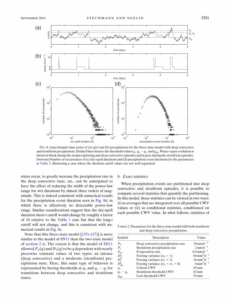
states occur, to greatly increase the precipitation rate in

the deep convective state, etc., can be anticipated to

have the effect of reducing the width of the power-law

range for wet durations by almost three orders of mag-

nitude. This is indeed consistent with numerical results

for the precipitation event duration seen in Fig. 8d, in

which there is effectively no detectable power-law

range. Similar considerations suggest that the dry-spell

duration short-t cutoff would change by roughly a factor

of 16 relative to the Table 1 case but that the long-t

cutoff will not change, and this is consistent with nu-

merical results in Fig. 8c.

Note that this three-state model [(35)–(37)] is more

similar to the model of SN11 than the two-state model

of section 2 is. The reason is that the model of SN11

allowedP*(q) andD1(q) to be q dependent with nearly

piecewise constant values of two types: an intense

(deep convective) and a moderate (stratiform) pre-

cipitation state. Here, this same type of behavior is

represented by having thresholds at qc and qc 2 q� for

transitions between deep convective and stratiform

states.

b. Exact statistics

When precipitation events are partitioned into deep

convective and stratiform episodes, it is possible to

compute several statistics that quantify the partitioning.

In this model, these statistics can be viewed in two ways:

(i) as averages that are integrated over all possible CWV

values or (ii) as conditional statistics, conditioned on

each possible CWV value. In what follows, statistics of

FIG. 8. (top) Sample time series of (a) q(t) and (b) precipitation for the three-state model with deep convective

and stratiform precipitation. Dashed lines denote the threshold values qc, qc2 q�, and qnp.Water vapor evolution is

shown in black during the nonprecipitating and deep convective episodes and in gray during the stratiformepisodes.

(bottom)Number of occurrences of (c) dry-spell durations and (d) precipitation event durations for the parameters

in Table 2, illustrating a case where the duration cutoff values are not well separated.

TABLE 2. Parameters for the three-statemodel with both stratiform

and deep convective precipitation.

Symbol Description Value

Pd Deep convective precipitation rate 10mmh21

Ps Stratiform precipitation rate 2mmh21

E* Evaporation rate 0.4mmh21

D2d Forcing variance (sd 5 1) 64mm2h21

D2s Forcing variance (ss 5 1) 16mm2h21

D2np Forcing variance (sd 5 ss 5 0) 8mm2h21

qc Critical CWV 65mm

qc 2 q� Stratiform threshold CWV 62mm

qnp Low-threshold CWV 53mm


these two types are presented in succession. (Derivations

are shown mostly in the appendix.)

As a first example of an integrated statistic, one can

consider the amount of time spent in each of the three

states. This is similar to a ‘‘cloud fraction’’ for each state

but computed over time domain without spatial con-

siderations, and only for precipitating cloud. For sim-

plicity, we use cloud fraction for this below (noting that

this would not be the same as cloud fraction treated in

a climate model radiative code). One obtains

nonprecipitating fraction5Pfsd 5 0,ss 5 0g

5FsPs/np

qc 2 qnp

Enp

, (40)

deep convection cloud fraction5Pfsd 5 1g5Fs

q�Pd

,

(41)

stratiform cloud fraction5Pfss5 1g

5FsPs/np

qc2 q� 2qnp

Ps

2FsPs/d

q�Ps

, (42)

where Fs enforces the normalization condition that

(40)–(42) sum to 1. For the parameters in Table 2, the

numerical values are Pfsd 5 0, ss 5 0g 5 0.89, Pfsd 51g5 0.016, and Pfss 5 1g5 0.098. From this, one finds

that the occurrence fraction of precipitation is Pfsd 51g1 Pfss5 1g5 0.11; of these occurrences, in turn, the

stratiform fraction Pfss 5 1g/(Pfsd 5 1g 1 Pfss 5 1g)is 0.86, which is close to the value of 0.84 reported by

Nesbitt et al. (2006) for mesoscale convective systems

over the ocean.

The quantities Ps/np and Ps/d that enter in (40)–(42)

are interesting statistics in and of themselves; they are

the probabilities of transition from the stratiform state

to either the nonprecipitating state or deep convection

state, respectively:

Ps/np 512 exp[2(2Ps/D

2s )q�]

12 exp[2(2Ps/D2s )(qc 2 qnp)]

, (43)

Ps/d5exp[2(2Ps/D

2s )q�]2 exp[2(2Ps/D

2s )(qc 2 qnp)]

12 exp[2(2Ps/D2s )(qc 2 qnp)]

,

(44)

which satisfy Ps/np 1 Ps/d 5 1. For the parameters

in Table 2, the numerical values are Ps/np 5 0.56 and

Ps/d5 0.44. The authors are not aware of any estimates

of these quantities from observational data.

In addition, the mean precipitation rate and the

stratiform rain fraction can be computed from (41) and

(42) as

hprecipi5PsPfss 5 1g1PdPfsd5 1g5FsPs/np(qc 2 qnp) (45)

and

stratiform rain fraction5PsPfss5 1ghprecipi . (46)

For the parameters in Table 2, the numerical values are

hprecipi 5 8.5mmday21 and stratiform rain fraction of

0.55. The hprecipi value is larger than the 5.4mmday21

recorded during Tropical Ocean and Global Atmo-

sphere Coupled Ocean–Atmosphere Response Experi-

ment (TOGA COARE) (Short et al. 1997) and the

5.3mmday21 recorded during the Kwajalein Experi-

ment (KWAJEX; Yuter et al. 2005), but it is similar to

the 9.9mmday21 measured during a particularly active

2-week period of TOGA COARE (Short et al. 1997).

The stratiform rain fraction of 0.55 is quite close to the

0.56 for the oceanic rainfall from Nesbitt et al. (2006);

however, this fraction can vary significantly in nature

[see Schumacher and Houze (2003) and references

therein].

A common aspect of the statistics (40)–(46) is that

they are averages over all possible water vapor values.

Specifically, they are related to the integrals

Pfsd5ss 5 0g5ðq

c

2‘pnp(q) dq , (47)

Pfsd 5 1g5ð‘qc2q

�

pd(q) dq , (48)

Pfss 5 1g5ðq

c

qnp

ps(q) dq , (49)

where pnp(q), pd(q), and ps(q) are the q-dependent

(stationary) probability densities of the three states. The

densities satisfy the overall normalization conditionð[pnp(q)1 pd(q)1ps(q)] dq5 1. (50)

Derivations of (40)–(46) are shown in the appendix.

Explicit formulas for pnp(q), pd(q), and ps(q) are derived

in the appendix, and they have a piecewise exponential

form, as shown in Fig. 9. To facilitate comparison with

Peters and Neelin (2006) and Neelin et al. (2009), Fig. 9

also shows the overall pdf of CWV [pnp(q) 1 pd(q) 1ps(q)] and the pdf of precipitating points [pd(q) 1 ps(q)].


These latter two pdfs are comparable to those from ob-

servational analyses, which are reproduced here in Fig. 1.

From these pdfs, one can see that the CWV is typically

below qc 5 65mm, even while precipitating, and the pdf

has a ‘‘long tail’’ with exponential decay above the critical

value. If a stochastic component to the transition threshold

were included, there would be a tendency to smooth out

these pdfs, similar to the discussion of Fig. 4. If the pre-

cipitation rate increased smoothly as a function of q over

the stratiform range, this would likewise yield a smoother

pdf. The presence of the lower-rain-rate stratiform range

(forDs as specified in Table 2) does produce an increase in

the pdf for precipitating points just below qc.

While (45) described the mean precipitation in-

tegrated over all possible q values, analogous statistics

can be found for particular q values. The mean and

second moment of precipitation, conditioned on column

water vapor value q, are

hprecipi(q)5 Psps(q)1Pdpd(q)

pnp(q)1 ps(q)1 pd(q), (51)

hprecip2i(q)5 P2s ps(q)1P2

dpd(q)

pnp(q)1 ps(q)1 pd(q). (52)

Figure 10 shows plots of the mean and the variance,

hprecip2i(q) 2 hprecipi2(q). The form has the same qual-

itative features as in the observational analysis of Peters

and Neelin (2006) and Neelin et al. (2009), as reproduced

here in Fig. 1: qc marks a rapid transition in the mean

precipitation and a peak in precipitation variance.

FIG. 9. CWV pdfs for the three-state model. (top) CWV pdfs

for the nonprecipitating state (gray), deep convection (solid

black), and stratiform (dashed black). (middle) Total pdf of CWV

(dashed) and pdf of CWV for the precipitating states (solid).

(bottom) As in (middle), except plotted with log-linear axis

scaling.

FIG. 10. Precipitation mean (dashed) and variance (solid) for the

three-state model with stratiform and deep convective pre-

cipitation. Similar considerations for precipitation variance above

qc apply as in Fig. 5.


Furthermore, the contributions to the mean pre-

cipitation [see (45)] can be displayed for each CWV:

How much rain falls at a given CWV value q? This

quantity could perhaps be called a ‘‘precipitation dis-

tribution function’’:

precipitation distribution5Psps(q)1Pdpd(q) . (53)

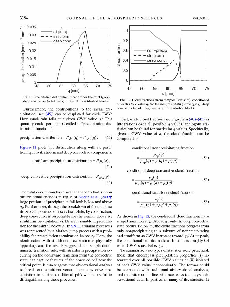
Figure 11 plots this distribution along with its parti-

tioning into stratiform and deep convective components:

stratiform precipitation distribution5Psps(q) ,

(54)

deep convective precipitation distribution5Pdpd(q) .

(55)

The total distribution has a similar shape to that seen in

observational analyses in Fig. 6 of Neelin et al. (2009):

large portions of precipitation fall both below and above

qc. Furthermore, through the breakdown of the total into

its two components, one sees that while, by construction,

deep convection is responsible for the rainfall above qc,

stratiform precipitation yields a reasonable representa-

tion for the rainfall below qc. In SN11, a similar hysteresis

was represented by a Markov jump process with a prob-

ability for precipitation termination below qc. Here, the

identification with stratiform precipitation is physically

appealing, and the results suggest that a simple deter-

ministic transition rule, with stratiform precipitation oc-

curring on the downward transition from the convective

state, can capture features of the observed pdf near the

critical point. It also suggests that observational analysis

to break out stratiform versus deep convective pre-

cipitation in similar conditional pdfs will be useful to

distinguish among these processes.

Last, while cloud fractions were given in (40)–(42) as

integrations over all possible q values, analogous sta-

tistics can be found for particular q values. Specifically,

given a CWV value of q, the cloud fraction can be

computed as

conditional nonprecipitating fraction

5pnp(q)

pnp(q)1 ps(q)1 pd(q), (56)

conditional deep convective cloud fraction

5pd(q)

pnp(q)1 ps(q)1 pd(q), (57)

conditional stratiform cloud fraction

5ps(q)

pnp(q)1 ps(q)1 pd(q). (58)

As shown in Fig. 12, the conditional cloud fractions have

a rapid transition at qc. Above qc, only the deep convective

state occurs. Below qc, the cloud fractions progress from

only nonprecipitating to a mixture of nonprecipitating

and stratiform as CWV increases toward qc. At its peak,

the conditional stratiform cloud fraction is roughly 0.4

when CWV is just below qc.

To summarize, two types of statistics were presented:

those that encompass precipitation properties (i) in-

tegrated over all possible CWV values or (ii) isolated

at each CWV value independently. The former could

be connected with traditional observational analyses,

and the latter are in line with new ways to analyze ob-

servational data. In particular, many of the statistics fit

FIG. 11. Precipitation distribution functions for the total (gray),

deep convective (solid black), and stratiform (dashed black). FIG. 12. Cloud fractions (from temporal statistics), conditioned

on each CWV value q, for the nonprecipitating state (gray), deep

convection (solid black), and stratiform (dashed black).


within the theme of the ‘‘transition to strong convec-

tion’’ (Neelin et al. 2009), and they also suggest, in ad-

dition to considering the temporal onset associated with

convective conditional instability, the importance of

also considering the reverse transition from strong con-

vection to stratiform precipitation upon moving down-

ward across the critical point.

6. Discussion

a. Additional statistics

In addition to the statistics presented here, further

statistics could also be computed analytically. Examples

include the event-size distribution for the three-state

model, the stratiform event-size distribution, and auto-

correlation functions. These statistics can be found an-

alytically using Laplace transforms, and they will be

presented elsewhere in the future.

b. Relation to renewal processes

As stated in section 1, the prototype models have the

form of renewal processes (Cox 1962). In such a process,

a state variable [here s(t) or sd(t) and ss(t)] makes

random transitions between states. The time intervals

between state transitions are determined by the event-

duration pdfs, which are pt0(t) and pt1(t) here for the

two-state model. In many precipitation models that can

be found in the literature, the form of these pdfs is as-

signed empirically based on observed data for pre-

cipitation alone. Here, in contrast, the form of pt0(t) and

pt1(t) arises from joint precipitation–water vapor dy-

namics. In other words, it is the water vapor dynamics,

interacting with a threshold, that is fundamental in the

prototype models here. The characterization as a re-

newal process is secondary, and it applies only to the

precipitation indicator s(t), not to the detailed water

vapor dynamics of q(t). Nevertheless, this characteriza-

tion as a renewal process can be useful for computing

marginal statistics of precipitation that do not rely on the

detailed evolution of the CWV; examples include the

precipitation-event-size distribution, the precipitation

autocorrelation function, etc.

c. Relation to ISCCP cloud regimes obtained fromcluster algorithms

It is tempting to compare the present paper’s model

statistics to empirically defined cloud regime data, such

as that defined from a cluster analysis of data from the

International Satellite Cloud Climatology Project

(ISCCP) (Jakob andTselioudis 2003; Rossow et al. 2005;

Jakob and Schumacher 2008). However, that cloud re-

gime analysis was based on data with a relatively large

footprint of O(280) km, whereas the present model

was aimed at analyses of data with a smaller footprint

ofO(20) km (Peters andNeelin 2006; Neelin et al. 2009).

In the future, perhaps this scale gap could be closed

somehow to allow a meaningful comparison.

d. Implications for convective parameterizations inGCMs

One interesting feature of the prototype models is the

element of hysteresis: after water vapor crosses above

qc, the precipitation event does not end when water

vapor returns to qc; instead, CWVmust fall to a second,

lower threshold qnp in order for precipitation to end.

This dynamics with two distinct thresholds—one for

onset and one for shutdown—is different from the trig-

gers used in many GCM convective parameterizations.

In many GCMs, a single threshold is used for both onset

and shutdown. The prototype models here offer simple

ways to include the hysteresis and multiple-threshold

behavior of convection.

A second interesting feature of the prototypes is the

important role of stratiform precipitation. In the two-

state model, with no distinction between deep con-

vective and stratiform precipitation, the CWVpdf gives

only a qualitative sketch of the observed features. For

instance, the maximum in Fig. 4 for precipitating points

occurs at the critical value rather than below. In the

three-state model, by partitioning deep convective and

stratiform precipitation, the realism of the statistics is

improved.

Based on these results, one would expect GCM con-

vective parameterizations to benefit from including a

stratiform component. Indeed, several studies have

demonstrated such benefits (Moncrieff and Liu 2006;

Khouider and Majda 2006; Khouider et al. 2011; Frenkel

et al. 2013), including a case with a stochastic param-

eterization (Biello et al. 2010; Frenkel et al. 2013). The

present prototypes offer simple ways to parameterize

a stratiform component. In particular, implementing

two or three thresholds—instead of just one—appears

to accomplish some aspects of this; and the stochastic

thresholds of Stechmann and Neelin (2011) offer an-

other simple alternative.

7. Conclusions

Two prototype models were presented for precipi-

tation and water vapor evolution. Among the goals,

a major aim was to understand the processes underlying

the joint statistics of precipitation and water vapor. To

this end, in the first prototype, a two-state model in-

volved a precipitating state and a nonprecipitating state

as a minimal representation of convective onset and


shutdown. In the other prototype, a three-state model

was introduced to partition precipitation events into

deep convective and stratiform episodes. Both pro-

totype models are exactly solvable for many quantities,

and analytical formulas were presented for model sta-

tistics. The tails of pdfs and the statistics of extreme

events can thus be described unambiguously, free from

statistical sampling errors, and insight can be obtained

into the governing physics.

As the simplest prototype, the two-state model was

seen to be sufficient for several basic features, including

in particular the precipitation-event-size distribution pS.

A prominent feature of pS was a range of power-law

scaling with exponent 23/2. This scaling was valid in be-

tween a characteristic small-event-size cutoff, b2P*/D21,

and a characteristic large-event-size cutoff,D21/P*. This

ratio D21/P* is also the characteristic scale of the ex-

ponential decay of the CWV pdf. This provides a use-

ful prototype for understanding several features of

event-size distributions seen in observations. Among

the most interesting are associated with the demon-

stration that stochastic forcing by variations in mois-

ture convergence driving moisture across a threshold

for the onset of rainfall is sufficient to set up a power-

law range with an exponent roughly similar to observa-

tional estimates. The key ingredients are the threshold,

the memory provided by the prognostic equation for

water vapor (or total water if condensate is included),

and the drift toward the threshold from both sides (by

evaporation from below and by precipitation from

above, each potentially modified by mean moisture

convergence).

This interpretation is consistent with prior discussion

(Peters et al. 2001; Peters and Neelin 2006) in terms

of self-organized criticality; the system is forced toward

the critical point from below, followed by an internal

dissipation mechanism that returns the system toward

the threshold from above. Indeed, first-passage pro-

cesses are among the simplest prototypes for self-

organized criticality (Redner 2001). Aspects gained

here are (i) the direct relationship to equations sim-

plified from meteorological models, (ii) a clear pro-

totype for how the time–domain interactions give the

power-law ranges in precipitation event and dry-spell

distributions and the cutoffs for these ranges, and

(iii) an understanding of the relationship between the

long tails above the critical point and the distributions

with power-law ranges. Regarding (ii), in seeking pro-

totype behavior for power-law ranges, one might be

tempted to conjecture that neighbor interactions in

the spatial domain could be essential to establishing the

set of properties near critical. While these might play a

role in spatial clustering properties, the present model

suggests that simple time–domain interactions involving

the onset threshold are the leading effect in establishing

the power-law range and in setting the difference in cutoff

values in event size or dry-event-duration distributions.

Regarding (iii), in typical prototype models for self-

organized criticality, as well as in standard assumptions

for convective quasi equilibrium, the system is tightly

confined just below critical [for a review, see Neelin et al.

(2008)] so the long tails observed for the distribution

of precipitating points above critical would appear

puzzling. In the two-state model, these long tails and

the large-event-size cutoff arise naturally together:

both are governed by the same scale and both depend

on the fluctuations of moisture convergence being

sufficiently large compared to the loss rate by precip-

itation. The power-law range for the dry-event dura-

tions arises by the flipside of this dynamics, with the

long-duration cutoff given by moisture convergence

fluctuations versus slow evaporative driving.

For precipitating-point water vapor distributions,

the two-state model gives results in which one can rec-

ognize key features of the observations but in highly

simplified form.Without including all the processes used

to reproduce these distributions in SN11, such as onset

probabilities, a three-state model is a natural next-most-

simple model and proves able to better capture a num-

ber of these features. The three-state model provides

formulas for the partitioning of precipitation into deep

convective and stratiform components, the latter simply

having a lower rain rate and an onset dictated by

downward transition from the deep convective state. In

addition to traditional statistics such as mean precip-

itation and stratiform cloud fraction, more detailed

versions were shown where, for instance, the contribu-

tions to total precipitation could be broken down for

each possible water vapor value q. This latter type of

statistic is in the spirit of the observational analyses of

Bretherton et al. (2002) and later Peters and Neelin

(2006) and Neelin et al. (2009), who identified a critical

value qc of water vapor that marks the transition to

strong convection. This provides a prototype for the

transition between strong convection and stratiform

precipitation near qc that suggests many aspects of this

can be captured in a simple time–domain formulation

that may be useful for parameterization.

Acknowledgments. The research of S.N.S. is partially

supported by the ONR Young Investigator Program

through Grant ONR N00014-12-1-0744, and J.D.N. is par-

tially supported by National Science Foundation Grant

AGS-1102838 and NOAA Grant NA11OAR4310099.

The authors thankA. Corral and T. Schneider for helpful

discussion.


APPENDIX A

Derivations for Two-State Model for ConvectiveOnset

a. Precipitation events

At the start of the precipitation event, the water vapor

is at its critical value q5 qc, and the event ends when the

water vapor has decreased to q 5 qnp. In this situation,

the pdf p1(q, t) for the water vapor evolves according to

a Fokker–Planck equation:

›tp1 2P*›qp15D2

1

2›2qp1 , (A1)

p1(qnp, t)5 0, (A2)

p1(q, 0)5 d(q2 qc) , (A3)

where the PDE is satisfied on qnp , q , ‘ with an ab-

sorbing boundary at q 5 qnp. The solution is

p1(q, t)51ffiffiffiffiffiffiffiffiffiffiffiffiffiffi

2pD21t

q8><>:exp

"2(q2 qc 1P*t)

2

2D21t

#

2 exp

2P*b

D21

!exp

2642(q2 qnp 1 b1P*t)

2

2D21t

3759>=>;

(A4)

(see Redner 2001). Since an event ends when the water

vapor reaches the threshold q5 qnp, the pdf pt1(t) of the

event duration is equivalent to the probability flux at the

threshold:

pt1(t)5

P*p11

D21

2

›p1›q

!��q5q

np

5D2

1

2

›p1›q

��q5q

np

, (A5)

which is given explicitly in (5).

b. Dry spells

At the start of a dry spell, the water vapor is at the low

threshold value q5 qnp, and the dry spell ends when the

water vapor has increased to q5 qc. In this situation, the

pdf p0(q, t) for the water vapor evolves according to

a Fokker–Planck equation:

›tp01E*›qp05D2

0

2›2qp0 , (A6)

p0(qc, t)5 0, (A7)

p0(q, 0)5 d(q2 qnp) , (A8)

where the PDE is satisfied on 2‘ , q , qc with an

absorbing boundary at q 5 qc. The solution is found

similarly to the wet-spell case but with some changes in

parameters.

c. Cloud fractions and stationary pdf

The equilibrium cloud fraction is defined in terms

of the probability densities p0(q) and p1(q) for the dry

and wet states at each CWV value q. In equilibrium,

the functions p0 and p1 satisfy the following system of

Fokker–Planck equations:

E*›qp05D2

0

2›2qp02 d(q2qnp)f1jq5q

np, 2‘, q, qc ,

(A9)

2P*›qp15D2

1

2›2qp11 d(q2 qc)f0jq5q

c, qnp ,q,‘ ,

(A10)

with absorbing boundary conditions

p0(qc)5 0, (A11)

p1(qnp)5 0, (A12)

and where f0 and f1 are the probability fluxes

f05E*p02D2

0

2›qp0 , (A13)

f152P*p12D2

1

2›qp1 . (A14)

The Dirac delta source terms in (A9) and (A10) rep-

resent transitions between the precipitating and non-

precipitating states at the absorbing boundaries, q 5 qcand q 5 qnp. Because of these Dirac delta source terms,

two types of consistency conditions arise. First, the

consistency condition

f0jq5qc52f1jq5q

np(A15)

or equivalently

2D2

0

2›qp0

��q5q

c

5D2

1

2›qp1

��q5q

np

(A16)

arises as a balance in the fluxes. This condition arises

from integrating (A9) and (A10) over their domains of

validity and assuming that p0 / 0 and ›qp0 / 0 as q/2‘ and that p1 / 0 and ›qp1 / 0 as q / ‘. The same

condition arises from both (A9) and (A10) for this two-

state system, and it represents an integrated balance in

the fluxes: the flux out of the dry state must be balanced


by a flux into the wet state and vice versa. Second, the

Dirac delta sources cause local jumps in the fluxes. The

jumps satisfy the consistency conditions

f0jq5q1np2 f0jq5q2

np52f1jq5q

np, (A17)

f1jq5q1c2 f1jq5q2

c5 f0jq5q

c

. (A18)

These conditions arise from integrating (A9) over the

small interval qnp 2 l , q , qnp 1 l and integrating

(A10) over the small interval qc 2 l , q , qc 1 l and

taking the limit as l / 0. As opposed to the integrated

flux balance in (A15), the conditions (A17) and (A18)

are local balances, at particular CWV values, between

an input flux and a jump in flux. Because of these jumps,

the functions p0(q) and p1(q) will be continuous but will

have jumps in their derivatives.

To solve for the stationary solution, one can first in-

tegrate (A9) and (A10) over each of the intervals2‘ ,q , qnp, qnp , q , qc, and qc , q , ‘. Within each of

these intervals, the Dirac delta terms are zero, the

equations are uncoupled, and p0(q) and p1(q) are ex-

ponential. Several integration constants arise, and their

values are determined by the following constraints: de-

cay of p0(q) and p1(q) and their derivatives as q tends

toward 6‘, the boundary conditions (A11) and (A12),

continuity of p0(q) at q 5 qnp and p1(q) at q 5 qc, the

jump conditions in (A17) and (A18), the integrated flux

balance conditions in (A15), and the overall normali-

zation condition in (23). In the end, the stationary so-

lution to (A9)–(A18) is piecewise exponential as written

explicitly in (24)–(27) and shown in Fig. 4.

APPENDIX B

Derivations for Three-State Model with StratiformPrecipitation

a. Stratiform events

Precipitation events now include both deep convec-

tive and stratiform rain, and they follow an alternating

sequence of events of the form deep–stratiform or deep–

stratiform–deep–stratiform or deep–stratiform–deep–

stratiform–deep–stratiform, etc. The deep convective

portions are determined in a similar way as in appendix

A, whereas the stratiform portions are considered next.

For a stratiform episode, CWV is initially at q5 qc 2q�, and the episode ends when CWV either decreases to

qnp or increases to qc. This evolution is described by the

following Fokker–Planck equation with two absorbing

boundaries:

›tps 2Ps›qps 5D2

s

2›2qps , (B1)

ps(qnp, t)5 0, (B2)

ps(qc, t)5 0, (B3)

ps(q, 0)5 d(q2qc 1 q�) , (B4)

where the PDE is satisfied on qnp , q , qc with ab-

sorbing boundaries at q5 qnp and q5 qc. At the start of

the stratiform event, the water vapor is at the value q 5qc 2 q�, which is the threshold for the end of a deep

convective episode.

Two quantities are of interest here: Ps/np and Ps/d.

These are the transition probabilities from the strati-

form state to the nonprecipitating and deep convective

states, respectively. In terms of the problem in (B1)–

(B4), Ps/np is the probability of first reaching the point

qnp, and Ps/d is the probability of first reaching the

point qc. This problem of first exit from an interval has

well-known solutions (Redner 2001; Gardiner 2004) that

are written explicitly in (43) and (44).

b. Cloud fractions and stationary pdf

The equilibrium cloud fractions are defined in terms

of the probability densities pnp(q), pd(q), and ps(q) for

the nonprecipitating, deep convective, and stratiform

states at each CWV value q. In equilibrium, the func-

tions pnp, pd, and ps satisfy the following system of

Fokker–Planck equations:

E*›qpnp 5D2

np

2›2qpnp 2 d(q2qnp)fsjq5q

npfor

2‘, q,qc , (B5)

2Pd›qpd 5D2

d

2›2qpd1 d(q2 qc)(fnpjq5q

c1 fsjq5q

c) for

qc2 q«, q,‘ ,

(B6)

2Ps›qps 5D2

s

2›2qps 2 d(q2 qc1 q�)fdjq5q

c2q

«for

qnp, q, qc ; (B7)

with absorbing boundary conditions

pnp(qc)5 0, (B8)

pd(qc2 q�)5 0, (B9)

ps(qc)5 ps(qnp)5 0; (B10)


and where fnp, fd, fs are the probability fluxes

fnp 5E*pnp 2D2

np

2›qpnp , (B11)

fd52Pdpd2D2

d

2›qpd , (B12)

fs 52Psps 2D2

s

2›qps . (B13)

The Dirac delta source terms in (B5)–(B7) represent

transitions between the states at their absorbing

boundaries. Because of these Dirac delta source terms,

two types of consistency conditions arise. First, the

consistency conditions

fnpjq5qc52fsjq5q

np, (B14)

2fdjq5qc2q

�5 fnpjq5q

c

1 fsjq5qc

, (B15)

fsjq5qc2 fsjq5q

np52fdjq5q

c2q

�(B16)

arise as balances in the fluxes. These conditions arise from

integrating (B5)–(B7) over their domains of validity and

assuming appropriate decay conditions as q / 6‘. Inessence, (B14)–(B16) represent integrated balance condi-

tions for fluxes into and out of each of the three states.

Second, the Dirac delta sources cause local jumps in the

fluxes. The jumps satisfy the consistency conditions

fnpjq5q1np2 fnpjq5q2

np52fsjq5q

np, (B17)

fdjq5q1c2 fdjq5q2

c5 fnpjq5q

c

1 fsjq5qc

, (B18)

fsjq5(qc2q

�)12 fsjq5(q

c2q

�)252fdjq5q

c2q

�. (B19)

These conditions arise from integrating (B5)–(B7) over

small intervals centered on the points qnp, qc, and qc2 q�,

respectively. For instance, (B17) is found by integrating

(B5) over the small interval qnp 2 l , q , qnp 1 l and

taking the limit as l / 0. As opposed to the integrated

flux balances in (B14)–(B16), the conditions (B17)–(B19)

are local balances, at particular CWV values, between an

input flux and a jump in a flux. Because of these jumps,

the functions pnp(q), pd(q), and ps(q) will be continuous

but will have jumps in their derivatives.

To solve for the stationary solution, one can first in-

tegrate (B5)–(B7) over each of the four intervals 2‘ ,q, qnp, qnp, q, qc2 q�, qc2 q�, q, qc, and qc, q,‘. Within each of these intervals, the Dirac delta terms

are zero, the equations are uncoupled, and the functions

pnp(q), pd(q), and ps(q) are exponential. Several in-

tegration constants arise, and their values are deter-

mined by the following constraints: decay of pnp(q),

pd(q), and ps(q) and their derivatives as q tends toward

6‘; the boundary conditions (B8)–(B10); continuity of

pnp(q) at q 5 qnp, pd(q) at q 5 qc, and ps(q) at q 5 qc 2q�; the jump conditions in (B17)–(B19); the integrated

flux balance conditions in (B14)–(B16); and the overall

normalization condition in (50). In the end, the sta-

tionary solution to (B5)–(B19) is piecewise exponential:

pnp(q)5Fnp

Enp

(12 exp

"22Enp

D2np

(qc 2 qnp)

#)exp

"2Enp

D2np

(q2qnp)

#for q, qnp , (B20)

pnp(q)5Fnp

Enp

(12 exp

"2Enp

D2np

(q2 qc)

#)for qnp , q, qc , (B21)

pd(q)5Fd

Pd

(12 exp

"22Pd

D2d

(q2 qc 1 q�)

#)for qc 2 q� , q, qc , (B22)

pd(q)5Fd

Pd

(12 exp

"22Pd

D2d

q«

#)exp

"22Pd

D2d

(q2 qc)

#for qc, q , (B23)

ps(q)5Fs

Ps

Ps/np

(12 exp

"22Ps

D2s

(q2qnp)

#)for qnp , q, qc 2q� , (B24)


ps(q)5Fs

Ps

Ps/d

(exp

"22Ps

D2s

(q2 qc)

#2 1

)for qc 2 q� , q, qc . (B25)

These functions are also plotted in Fig. 9. The quantities

Ps/np and Ps/d are the transition probabilities given in

(43) and (44). The quantities Fnp, Fd, and Fs are the input

fluxes into the nonprecipitating, deep convective, and

stratiform states, respectively. They are defined by the

right-hand sides of (B14)–(B16), respectively, and il-

lustrated schematically in Fig. 6. Their explicit values are

Fnp5FsPs/np , (B26)

Fd 5Fs , (B27)

Fs5

Ps/np

qc 2 qnp

Enp

1q�Pd

1Ps/np

qc2 q� 2qnp

Ps

2Ps/d

q�Ps

!21, (B28)

where Fs also arises as the normalization constant for the

cloud fractions in (40)–(42).

REFERENCES

Andrade, R. F. S., H. J. Schellnhuber, and M. Claussen, 1998:

Analysis of rainfall records: Possible relation to self-organized

criticality. Physica A, 254 (3–4), 557–568, doi:10.1016/

S0378-4371(98)00057-0.

Arakawa, A., and W. H. Schubert, 1974: Interaction of a cumulus

cloud ensemble with the large-scale environment, Part I. J. At-

mos. Sci., 31, 674–701, doi:10.1175/1520-0469(1974)031,0674:

IOACCE.2.0.CO;2.

Bernardara, P., C.DeMichele, andR.Rosso, 2007:A simplemodel

of rain in time: An alternating renewal process of wet and dry

states with a fractional (non-Gaussian) rain intensity. Atmos.

Res., 84, 291–301, doi:10.1016/j.atmosres.2006.09.001.

Betts, A. K., 1986: A new convective adjustment scheme. Part I:

Observational and theoretical basis. Quart. J. Roy. Meteor.

Soc., 112, 677–692.Biello J. A., B. Khouider, and A. J. Majda, 2010: A stochastic

multicloud model for tropical convection. Commun. Math.

Sci., 8, 187–216, doi:10.4310/CMS.2010.v8.n1.a10.

Bretherton, C. S., M. E. Peters, and L. E. Back, 2002: Relationships

between water vapor path and precipitation over the

tropical oceans. J. Climate, 15, 2907–2920, doi:10.1175/

1520-0442(2002)015,2907:ASMOAC.2.0.CO;2.

Cheng, C.-P., and R. A. Houze Jr., 1979: The distribution of con-

vective and mesoscale precipitation in GATE radar echo

patterns. Mon. Wea. Rev., 107, 1370–1381, doi:10.1175/

1520-0493(1979)107,1370:TDOCAM.2.0.CO;2.

Christensen,K., andN.R.Moloney, 2005:Complexity andCriticality.

Imperial College Press, 392 pp.

Cox, D. R., 1962: Renewal Theory. Methuen, 142 pp.

Foufoula-Georgiou, E., and D. P. Lettenmaier, 1987: A Markov

renewalmodel for rainfall occurrences.Water Resour. Res., 23,

875–884, doi:10.1029/WR023i005p00875.

Frenkel, Y., A. J. Majda, and B. Khouider, 2013: Stochastic and

deterministic multicloud parameterizations for tropical

convection. Climate Dyn., 41, 1527–1551, doi:10.1007/

s00382-013-1678-z.

Galewsky, J., A. Sobel, and I. Held, 2005: Diagnosis of subtropical

humidity dynamics using tracers of last saturation. J. Atmos.

Sci., 62, 3353–3367, doi:10.1175/JAS3533.1.

Gardiner, C. W., 2004: Handbook of Stochastic Methods: For

Physics, Chemistry, and the Natural Sciences. Springer Series

in Synergetics, Vol. 13, Springer-Verlag, 442 pp.

Green, J. R., 1964: A model for rainfall occurrence. J. Roy. Stat.

Soc., 26B, 345–353.

Hilburn, K. A., and F. J. Wentz, 2008: Intercalibrated passive mi-

crowave rain products from the unified microwave ocean re-

trieval algorithm (UMORA). J. Appl. Meteor. Climatol., 47,

778–794, doi:10.1175/2007JAMC1635.1.

Holloway, C. E., and J. D.Neelin, 2009:Moisture vertical structure,

column water vapor, and tropical deep convection. J. Atmos.

Sci., 66, 1665–1683, doi:10.1175/2008JAS2806.1.

Houze, R. A., Jr., 1989: Observed structure of mesoscale convective

systems and implications for large-scale heating.Quart. J. Roy.

Meteor. Soc., 115, 425–461, doi:10.1002/qj.49711548702.Jakob, C., andG. Tselioudis, 2003: Objective identification of cloud

regimes in the tropical western Pacific.Geophys. Res. Lett., 30,

2082, doi:10.1029/2003GL018367.

——, and C. Schumacher, 2008: Precipitation and latent heating

characteristics of themajor tropicalwesternPacific cloud regimes.

J. Climate, 21, 4348–4364, doi:10.1175/2008JCLI2122.1.

Khouider, B., and A. J. Majda, 2006: A simple multicloud param-

eterization for convectively coupled tropical waves. Part I:

Linear analysis. J. Atmos. Sci., 63, 1308–1323, doi:10.1175/

JAS3677.1.

——, and ——, 2008: Equatorial convectively coupled waves in

a simple multicloud model. J. Atmos. Sci., 65, 3376–3397,

doi:10.1175/2008JAS2752.1.

——, A. St-Cyr, A. J. Majda, and J. Tribbia, 2011: The MJO and

convectively coupled waves in a coarse-resolution GCM with

a simple multicloud parameterization. J. Atmos. Sci., 68, 240–

264, doi:10.1175/2010JAS3443.1.

Majda, A. J., and B. Khouider, 2002: Stochastic and mesoscopic

models for tropical convection. Proc. Natl. Acad. Sci. USA, 99,

1123–1128, doi:10.1073/pnas.032663199.

——, and S. N. Stechmann, 2008: Stochastic models for convective

momentum transport.Proc. Natl. Acad. Sci. USA, 105, 17 614–

17 619, doi:10.1073/pnas.0806838105.

——, and ——, 2009: A simple dynamical model with features of

convective momentum transport. J. Atmos. Sci., 66, 373–392,

doi:10.1175/2008JAS2805.1.

Mapes, B. E., 1993: Gregarious tropical convection. J. Atmos.

Sci., 50, 2026–2037, doi:10.1175/1520-0469(1993)050,2026:

GTC.2.0.CO;2.

——, 2000: Convective inhibition, subgrid-scale triggering energy,

and stratiform instability in a toy tropical wave model. J. At-

mos. Sci., 57, 1515–1535, doi:10.1175/1520-0469(2000)057,1515:

CISSTE.2.0.CO;2.


http://dx.doi.org/10.1016/S0378-4371(98)00057-0

http://dx.doi.org/10.1016/S0378-4371(98)00057-0

http://dx.doi.org/10.1175/1520-0469(1974)031<0674:IOACCE>2.0.CO;2

http://dx.doi.org/10.1175/1520-0469(1974)031<0674:IOACCE>2.0.CO;2

http://dx.doi.org/10.1016/j.atmosres.2006.09.001

http://dx.doi.org/10.4310/CMS.2010.v8.n1.a10

http://dx.doi.org/10.1175/1520-0442(2002)015<2907:ASMOAC>2.0.CO;2

http://dx.doi.org/10.1175/1520-0442(2002)015<2907:ASMOAC>2.0.CO;2

http://dx.doi.org/10.1175/1520-0493(1979)107<1370:TDOCAM>2.0.CO;2

http://dx.doi.org/10.1175/1520-0493(1979)107<1370:TDOCAM>2.0.CO;2

http://dx.doi.org/10.1029/WR023i005p00875

http://dx.doi.org/10.1007/s00382-013-1678-z

http://dx.doi.org/10.1007/s00382-013-1678-z

http://dx.doi.org/10.1175/JAS3533.1

http://dx.doi.org/10.1175/2007JAMC1635.1

http://dx.doi.org/10.1175/2008JAS2806.1

http://dx.doi.org/10.1002/qj.49711548702

http://dx.doi.org/10.1029/2003GL018367

http://dx.doi.org/10.1175/2008JCLI2122.1





http://dx.doi.org/10.1073/pnas.032663199

http://dx.doi.org/10.1073/pnas.0806838105


http://dx.doi.org/10.1175/1520-0469(1993)050<2026:GTC>2.0.CO;2

http://dx.doi.org/10.1175/1520-0469(1993)050<2026:GTC>2.0.CO;2

http://dx.doi.org/10.1175/1520-0469(2000)057<1515:CISSTE>2.0.CO;2

http://dx.doi.org/10.1175/1520-0469(2000)057<1515:CISSTE>2.0.CO;2

Moncrieff, M. W., and C. Liu, 2006: Representing convective or-

ganization in predictionmodels by a hybrid strategy. J. Atmos.

Sci., 63, 3404–3420, doi:10.1175/JAS3812.1.

Muller, C., L. Back, P. O’Gorman, and K. Emanuel, 2009: Amodel

for the relationship between tropical precipitation and column

water vapor. Geophys. Res. Lett., 36, L16804, doi:10.1029/

2009GL039667.

Neelin, J. D., O. Peters, J.W.-B. Lin, K. Hales, and C. E. Holloway,

2008: Rethinking convective quasi-equilibrium:Observational

constraints for stochastic convective schemes in climate

models. Philos. Trans. Roy. Soc. London, A366, 2581–2604,

doi:10.1098/rsta.2008.0056.

——,——, andK. Hales, 2009: The transition to strong convection.

J. Atmos. Sci., 66, 2367–2384, doi:10.1175/2009JAS2962.1.

Nesbitt, S. W., R. Cifelli, and S. A. Rutledge, 2006: Storm mor-

phology and rainfall characteristics of TRMM precipitation

features. Mon. Wea. Rev., 134, 2702–2721, doi:10.1175/

MWR3200.1.

O’Gorman, P. A., and T. Schneider, 2006: Stochastic models for

the kinematics of moisture transport and condensation in

homogeneous turbulent flows. J. Atmos. Sci., 63, 2992–3005,

doi:10.1175/JAS3794.1.

——, N. Lamquin, T. Schneider, and M. S. Singh, 2011: The

relative humidity in an isentropic advection–condensation

model: Limited poleward influence and properties of sub-

tropical minima. J. Atmos. Sci., 68, 3079–3093, doi:10.1175/JAS-D-11-067.1.

Peters, O., and J. D. Neelin, 2006: Critical phenomena in atmo-

spheric precipitation. Nat. Phys., 2, 393–396, doi:10.1038/

nphys314.

——, C. Hertlein, and K. Christensen, 2001: A complexity view

of rainfall. Phys. Rev. Lett., 88, 018701, doi:10.1103/

PhysRevLett.88.018701.

——,A. Deluca, A. Corral, J. D. Neelin, and C. E. Holloway, 2010:

Universality of rain event size distributions. J. Stat. Mech.,

2010, P11030, doi:10.1088/1742-5468/2010/11/P11030.

Pierrehumbert, R. T., 1998: Lateral mixing as a source of sub-

tropical water vapor. Geophys. Res. Lett., 25, 151–154,

doi:10.1029/97GL03563.

——, H. Brogniez, and R. Roca, 2007: On the relative humidity of

the earth’s atmosphere. The Global Circulation of the Atmo-

sphere: Phenomena, Theory, Challenges, T. Schneider and

A. H. Sobel, Eds., Princeton University Press, 143–185.

Ratan, R., and V. Venugopal, 2013: Wet and dry spell character-

istics of global tropical rainfall. Water Resour. Res., 49, 3830–3841, doi:10.1002/wrcr.20275.

Redner, S., 2001: A Guide to First-Passage Processes. Cambridge

University Press, 328 pp.

Rickenbach, T. M., and S. A. Rutledge, 1998: Convection in

TOGA COARE: Horizontal scale, morphology, and rain-

fall production. J. Atmos. Sci., 55, 2715–2729, doi:10.1175/

1520-0469(1998)055,2715:CITCHS.2.0.CO;2.

Roldán, J., andD.A.Woolhiser, 1982: Stochastic daily precipitation

models: 1. A comparison of occurrence processes. Water Re-

sour. Res., 18, 1451–1459, doi:10.1029/WR018i005p01451.

Rossow, W. B., G. Tselioudis, A. Polak, and C. Jakob, 2005:

Tropical climate described as a distribution of weather states

indicated by distinct mesoscale cloud property mixtures. Geo-

phys. Res. Lett., 32, L21812, doi:10.1029/2005GL024584.

Schmitt, F., S. Vannitsem, and A. Barbosa, 1998: Modeling of

rainfall time series using two-state renewal processes and

multifractals. J. Geophys. Res., 103 (D18), 23 181–23 193,

doi:10.1029/98JD02071.

Schumacher, C., and R. A. Houze Jr., 2003: Stratiform rain in

the tropics as seen by the TRMM Precipitation Radar. J. Cli-

mate, 16, 1739–1756, doi:10.1175/1520-0442(2003)016,1739:

SRITTA.2.0.CO;2.

——, ——, and I. Kraucunas, 2004: The tropical dynamical re-

sponse to latent heating estimates derived from the TRMM

precipitation radar. J. Atmos. Sci., 61, 1341–1358, doi:10.1175/

1520-0469(2004)061,1341:TTDRTL.2.0.CO;2.

Short, D. A., P. A. Kucera, B. S. Ferrier, J. C. Gerlach, S. A.

Rutledge, and O. W. Thiele, 1997: Shipboard radar rainfall

patterns within the TOGACOARE IFA.Bull. Amer. Meteor.

Soc., 78, 2817–2836, doi:10.1175/1520-0477(1997)078,2817:

SRRPWT.2.0.CO;2.

Sornette, D., 2004: Critical Phenomena in Natural Sciences.

Springer Verlag, 528 pp.

Stechmann, S. N., and A. J. Majda, 2009: Gravity waves in shear

and implications for organized convection. J. Atmos. Sci., 66,

2579–2599, doi:10.1175/2009JAS2976.1.

——, and J. D. Neelin, 2011: A stochastic model for the transition

to strong convection. J. Atmos. Sci., 68, 2955–2970,

doi:10.1175/JAS-D-11-028.1.

Steiner, M., R. A. Houze Jr., and S. E. Yuter, 1995: Climatological

characterization of three-dimensional storm structure

from operational radar and rain gauge data. J. Appl. Me-

teor., 34, 1978–2007, doi:10.1175/1520-0450(1995)034,1978:

CCOTDS.2.0.CO;2.

Sukhatme, J., andW.R. Young, 2011: The advection–condensation

model and water-vapour probability density functions.Quart.

J. Roy. Meteor. Soc., 137, 1561–1572, doi:10.1002/qj.869.

Tulich, S. N., D. Randall, and B. Mapes, 2007: Vertical-mode and

cloud decomposition of large-scale convectively coupled

gravity waves in a two-dimensional cloud-resolving model.

J. Atmos. Sci., 64, 1210–1229, doi:10.1175/JAS3884.1.

Yano, J.-I., C. Liu, and M. W. Moncrieff, 2012: Self-organized

criticality and homeostasis in atmospheric convective

organization. J. Atmos. Sci., 69, 3449–3462, doi:10.1175/

JAS-D-12-069.1.

Yuter, S. E., R. A. Houze Jr., E. A. Smith, T. T. Wilheit, and

E. Zipser, 2005: Physical characterization of tropical oceanic

convection observed in KWAJEX. J. Appl. Meteor., 44, 385–

415, doi:10.1175/JAM2206.1.



http://dx.doi.org/10.1029/2009GL039667

http://dx.doi.org/10.1029/2009GL039667

http://dx.doi.org/10.1098/rsta.2008.0056


http://dx.doi.org/10.1175/MWR3200.1

http://dx.doi.org/10.1175/MWR3200.1


http://dx.doi.org/10.1175/JAS-D-11-067.1


http://dx.doi.org/10.1038/nphys314

http://dx.doi.org/10.1038/nphys314

http://dx.doi.org/10.1103/PhysRevLett.88.018701

http://dx.doi.org/10.1103/PhysRevLett.88.018701

http://dx.doi.org/10.1088/1742-5468/2010/11/P11030

http://dx.doi.org/10.1029/97GL03563

http://dx.doi.org/10.1002/wrcr.20275

http://dx.doi.org/10.1175/1520-0469(1998)055<2715:CITCHS>2.0.CO;2

http://dx.doi.org/10.1175/1520-0469(1998)055<2715:CITCHS>2.0.CO;2

http://dx.doi.org/10.1029/WR018i005p01451

http://dx.doi.org/10.1029/2005GL024584

http://dx.doi.org/10.1029/98JD02071

http://dx.doi.org/10.1175/1520-0442(2003)016<1739:SRITTA>2.0.CO;2

http://dx.doi.org/10.1175/1520-0442(2003)016<1739:SRITTA>2.0.CO;2

http://dx.doi.org/10.1175/1520-0469(2004)061<1341:TTDRTL>2.0.CO;2

http://dx.doi.org/10.1175/1520-0469(2004)061<1341:TTDRTL>2.0.CO;2

http://dx.doi.org/10.1175/1520-0477(1997)078<2817:SRRPWT>2.0.CO;2

http://dx.doi.org/10.1175/1520-0477(1997)078<2817:SRRPWT>2.0.CO;2



http://dx.doi.org/10.1175/1520-0450(1995)034<1978:CCOTDS>2.0.CO;2

http://dx.doi.org/10.1175/1520-0450(1995)034<1978:CCOTDS>2.0.CO;2

http://dx.doi.org/10.1002/qj.869




http://dx.doi.org/10.1175/JAM2206.1

First-Passage-Time Prototypes for Precipitation Statistics

Documents

Transcript of First-Passage-Time Prototypes for Precipitation Statistics