First-Order Knowledge Compilation - UCLAweb.cs.ucla.edu/~guyvdb/talks/Dagstuhl17.pdf · First-Order...
181
First-Order Knowledge Compilation Guy Van den Broeck Dagstuhl Sept 18, 2017
Transcript of First-Order Knowledge Compilation - UCLAweb.cs.ucla.edu/~guyvdb/talks/Dagstuhl17.pdf · First-Order...
First-Order
Knowledge Compilation
Guy Van den Broeck
Dagstuhl
Sept 18, 2017
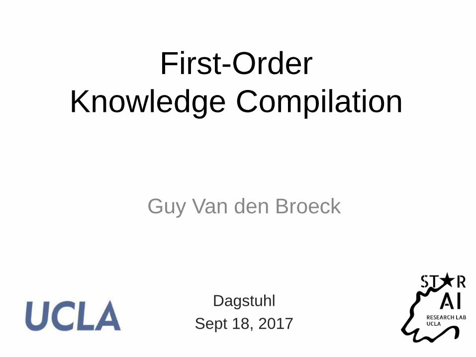
Overview
1. Propositional Refresher
2. Primer: A First-Order Tractable Language
3. Probabilistic Databases
4. Symmetric First-Order Model Counting
5. Lots of Pointers
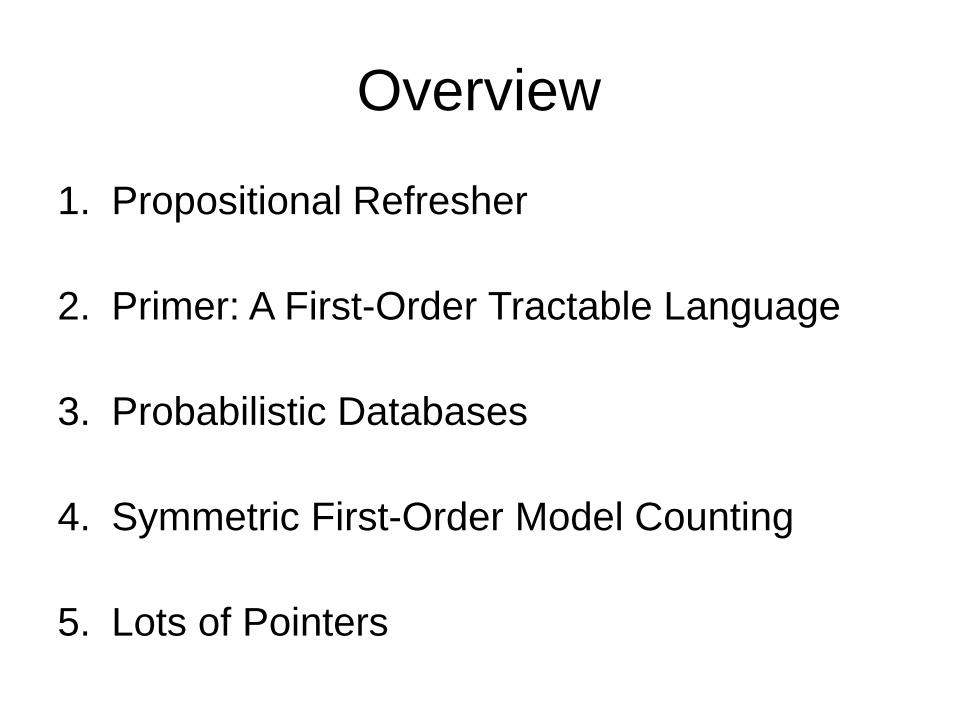
Overview
1. Propositional Refresher
2. Primer: A First-Order Tractable Language
3. Probabilistic Databases
4. Symmetric First-Order Model Counting
5. Lots of Pointers
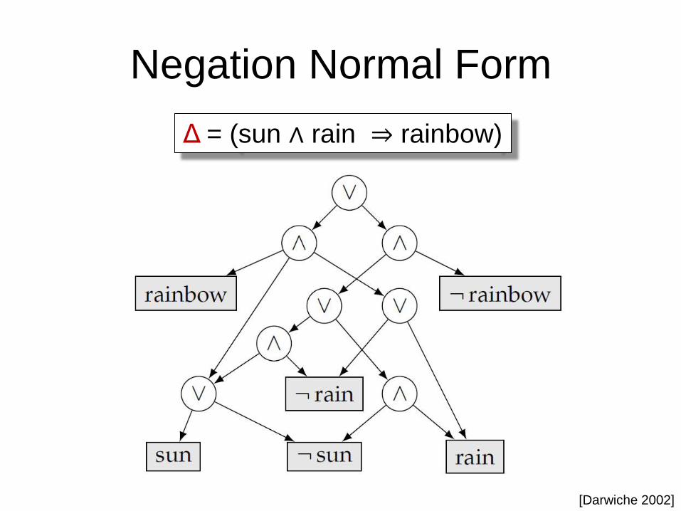
Negation Normal Form
[Darwiche 2002]
Δ = (sun ∧ rain ⇒ rainbow)
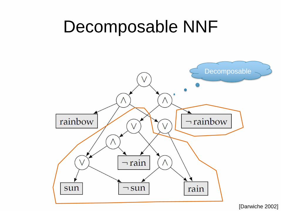
Decomposable NNF
Decomposable
[Darwiche 2002]
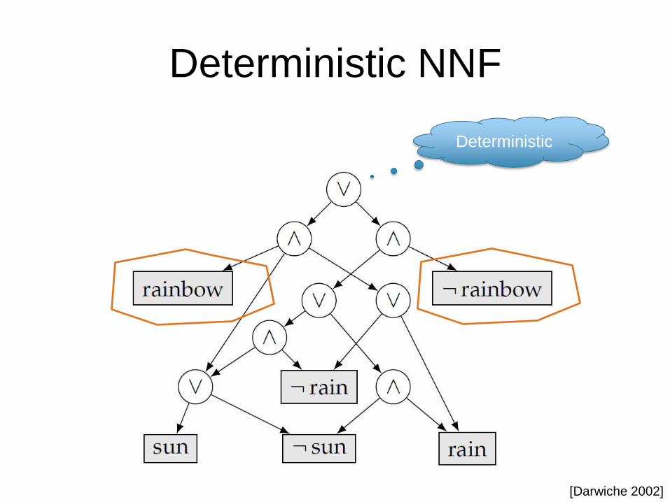
Deterministic NNF
Deterministic
[Darwiche 2002]
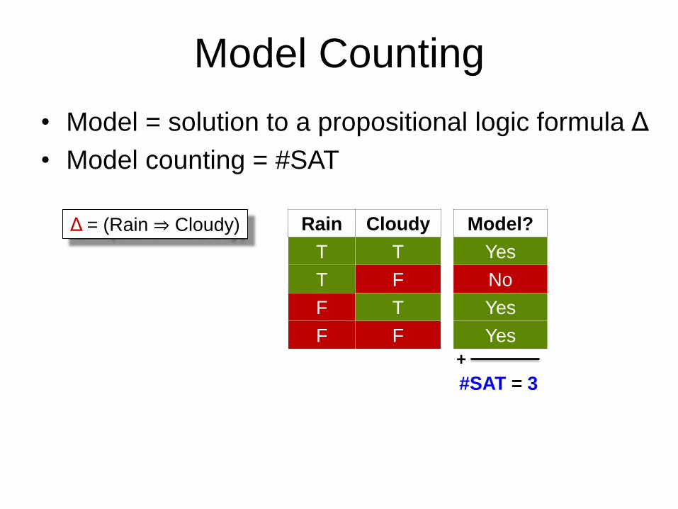
Model Counting
• Model = solution to a propositional logic formula Δ
• Model counting = #SAT
Rain Cloudy Model?
T T Yes
T F No
F T Yes
F F Yes
#SAT = 3
+
Δ = (Rain ⇒ Cloudy)
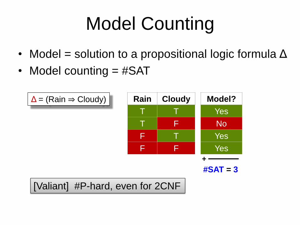
Model Counting
• Model = solution to a propositional logic formula Δ
• Model counting = #SAT
Rain Cloudy Model?
T T Yes
T F No
F T Yes
F F Yes
#SAT = 3
+
Δ = (Rain ⇒ Cloudy)
[Valiant] #P-hard, even for 2CNF
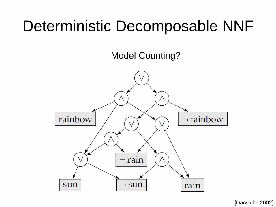
Deterministic Decomposable NNF
Model Counting?
[Darwiche 2002]
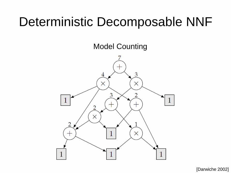
Deterministic Decomposable NNF
Model Counting
[Darwiche 2002]
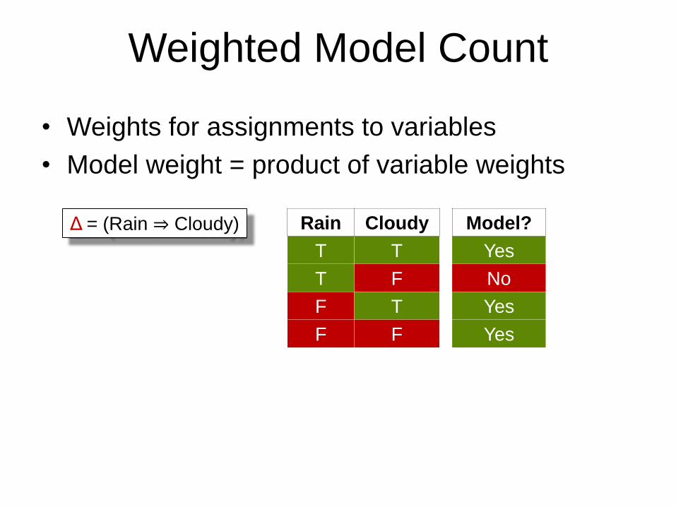
Weighted Model Count
• Weights for assignments to variables
• Model weight = product of variable weights
Rain Cloudy Model?
T T Yes
T F No
F T Yes
F F Yes
Δ = (Rain ⇒ Cloudy)

Weighted Model Count
• Weights for assignments to variables
• Model weight = product of variable weights
Rain
w(R) w(¬R)
1 2
Cloudy
w(C) w(¬C)
3 5
Rain Cloudy Model?
T T Yes
T F No
F T Yes
F F Yes
Δ = (Rain ⇒ Cloudy)
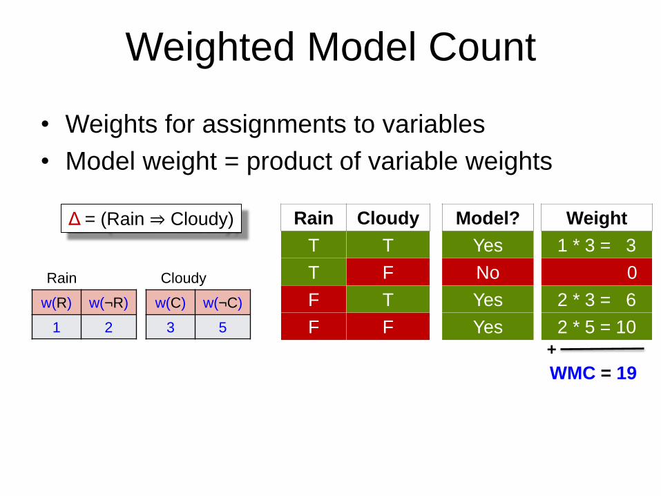
Weighted Model Count
Weight
1 * 3 = 3
0
2 * 3 = 6
2 * 5 = 10
WMC = 19
• Weights for assignments to variables
• Model weight = product of variable weights
+
Rain
w(R) w(¬R)
1 2
Cloudy
w(C) w(¬C)
3 5
Rain Cloudy Model?
T T Yes
T F No
F T Yes
F F Yes
Δ = (Rain ⇒ Cloudy)
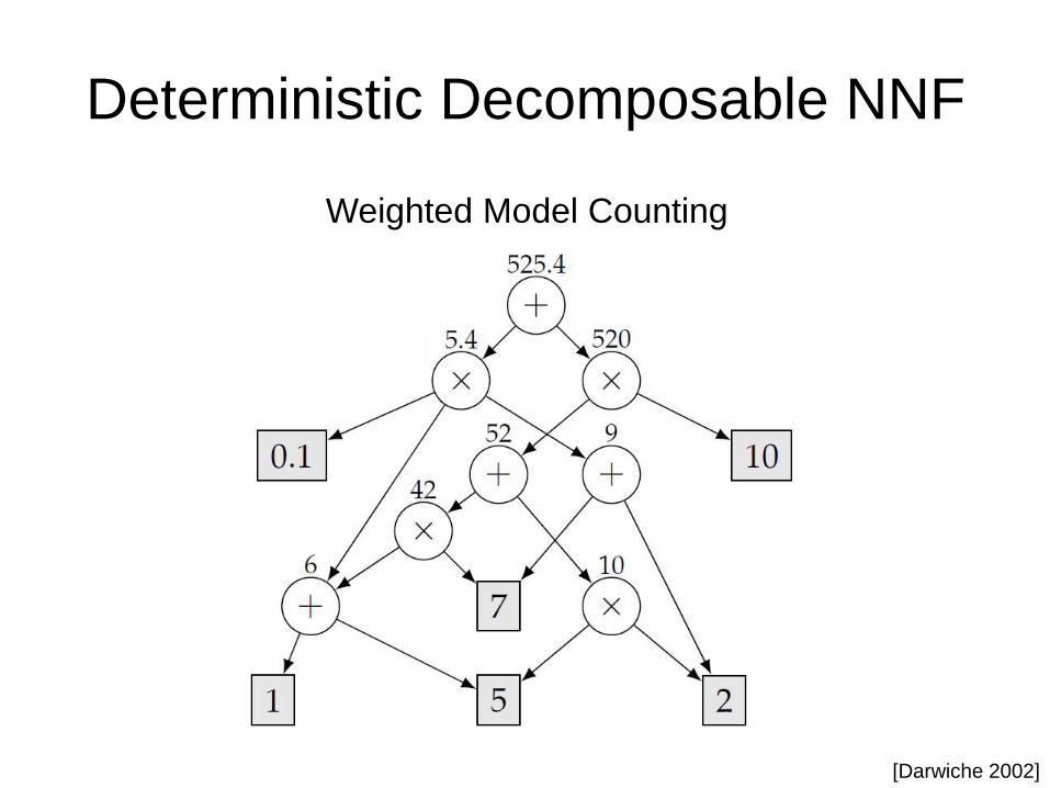
Deterministic Decomposable NNF
Weighted Model Counting
[Darwiche 2002]
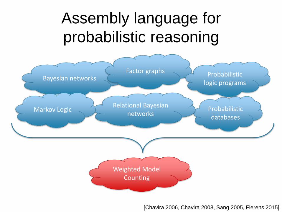
Assembly language for
probabilistic reasoning
Bayesian networks Factor graphs
Probabilistic databases
Relational Bayesian networks
Probabilistic logic programs
Markov Logic
Weighted Model Counting
[Chavira 2006, Chavira 2008, Sang 2005, Fierens 2015]
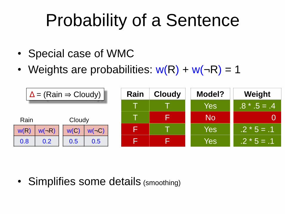
Probability of a Sentence
Weight
.8 * .5 = .4
0
.2 * 5 = .1
.2 * 5 = .1
• Special case of WMC
• Weights are probabilities: w(R) + w(¬R) = 1
• Simplifies some details (smoothing)
Rain
w(R) w(¬R)
0.8 0.2
Cloudy
w(C) w(¬C)
0.5 0.5
Rain Cloudy Model?
T T Yes
T F No
F T Yes
F F Yes
Δ = (Rain ⇒ Cloudy)
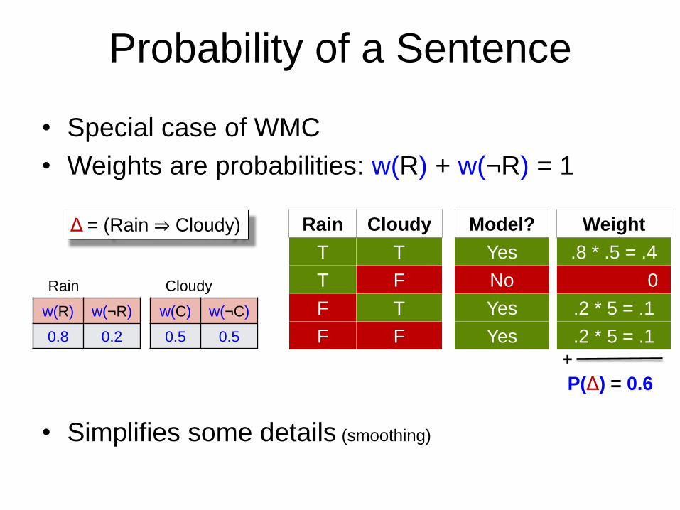
Probability of a Sentence
Weight
.8 * .5 = .4
0
.2 * 5 = .1
.2 * 5 = .1
P(Δ) = 0.6
• Special case of WMC
• Weights are probabilities: w(R) + w(¬R) = 1
• Simplifies some details (smoothing)
+
Rain
w(R) w(¬R)
0.8 0.2
Cloudy
w(C) w(¬C)
0.5 0.5
Rain Cloudy Model?
T T Yes
T F No
F T Yes
F F Yes
Δ = (Rain ⇒ Cloudy)
Overview
1. Propositional Refresher
2. Primer: A First-Order Tractable Language
3. Probabilistic Databases
4. Symmetric First-Order Model Counting
5. Lots of Pointers
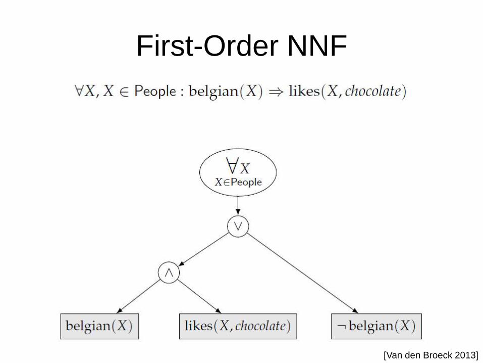
First-Order NNF
[Van den Broeck 2013]
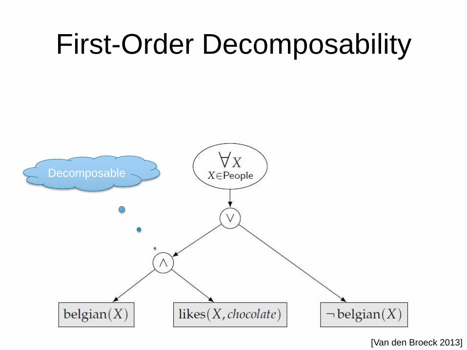
First-Order Decomposability
Decomposable
[Van den Broeck 2013]
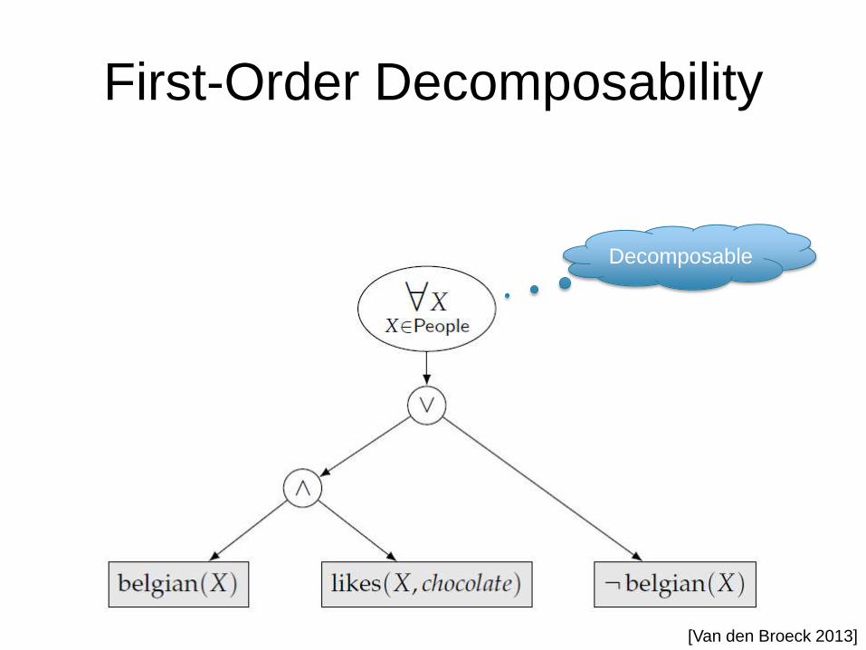
First-Order Decomposability
Decomposable
[Van den Broeck 2013]
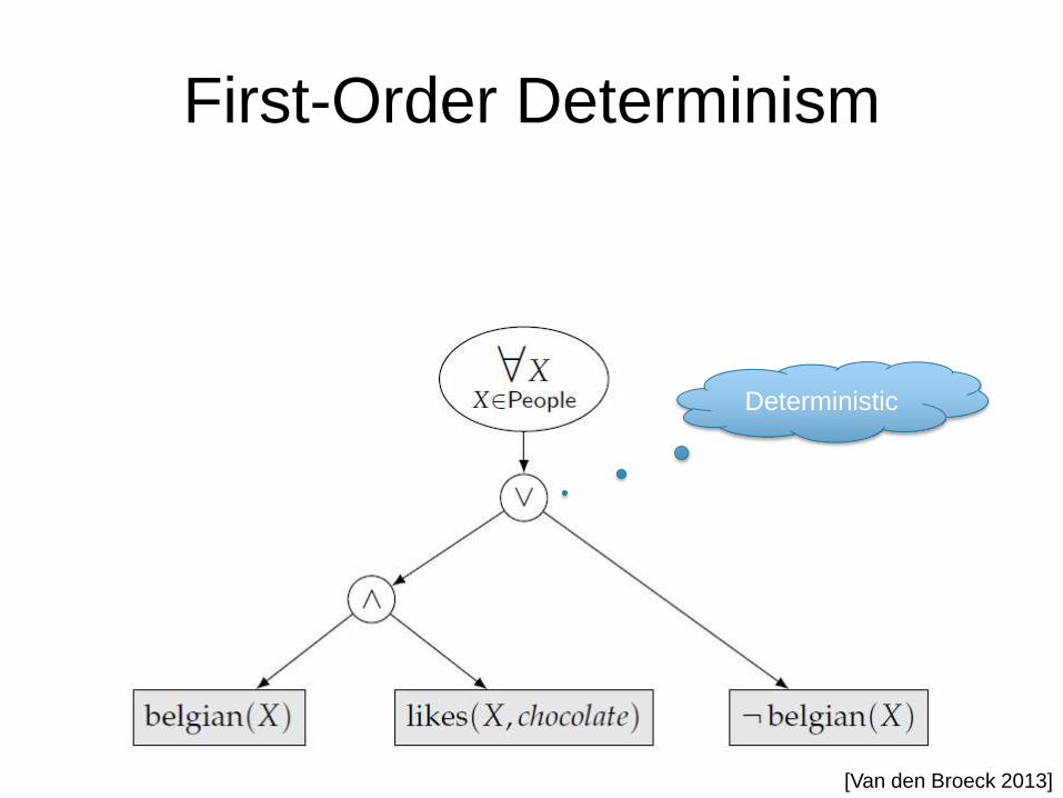
First-Order Determinism
Deterministic
[Van den Broeck 2013]
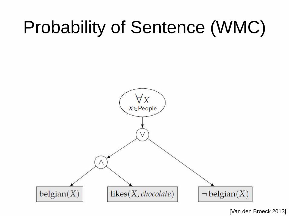
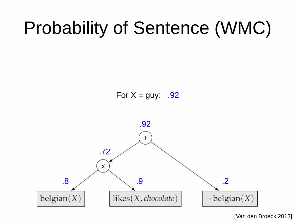
Probability of Sentence (WMC)
[Van den Broeck 2013]
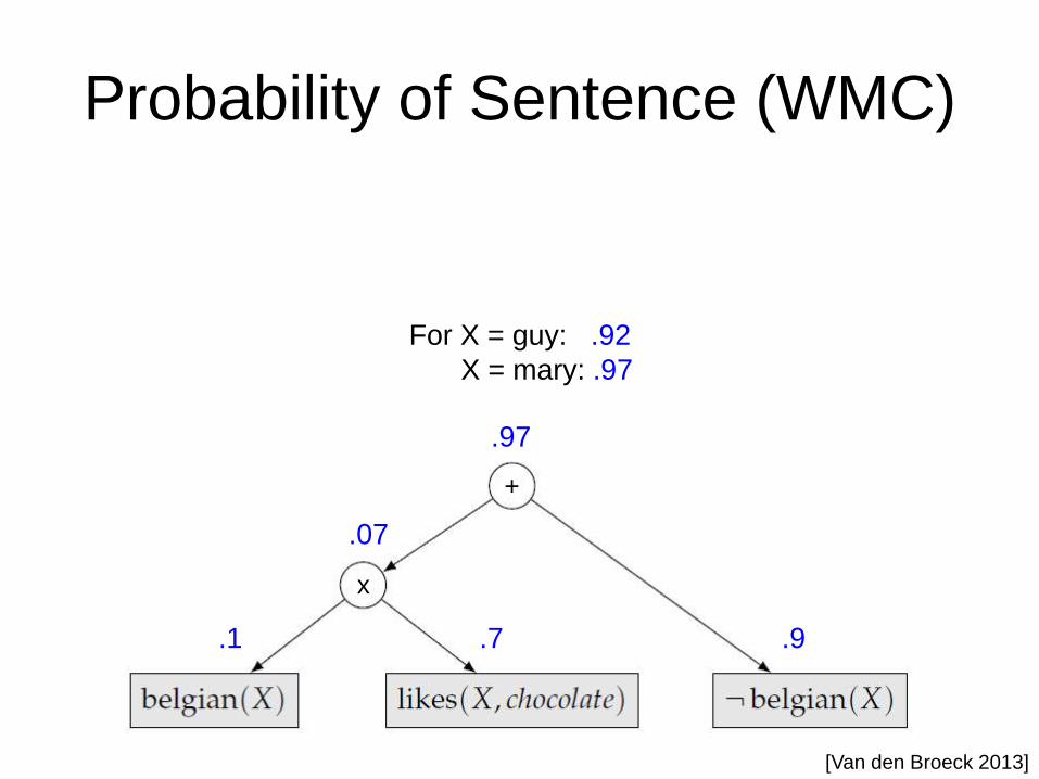
Probability of Sentence (WMC)
[Van den Broeck 2013]
For X = guy: .92
.8 .9 .2
.72
x
+
.92
Probability of Sentence (WMC)
[Van den Broeck 2013]
For X = guy: .92
X = mary: .97
.1 .7 .9
.07
x
+
.97
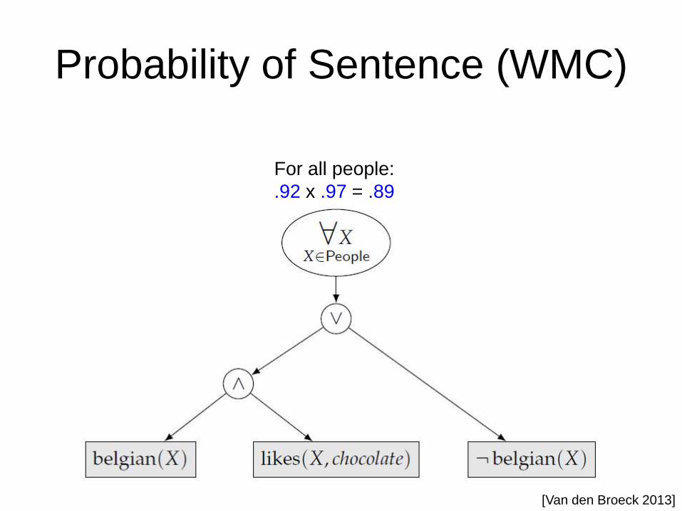
Probability of Sentence (WMC)
[Van den Broeck 2013]
For all people:
.92 x .97 = .89
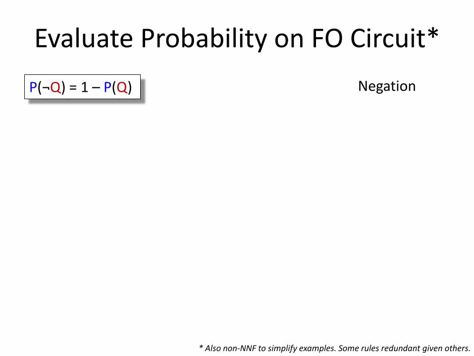
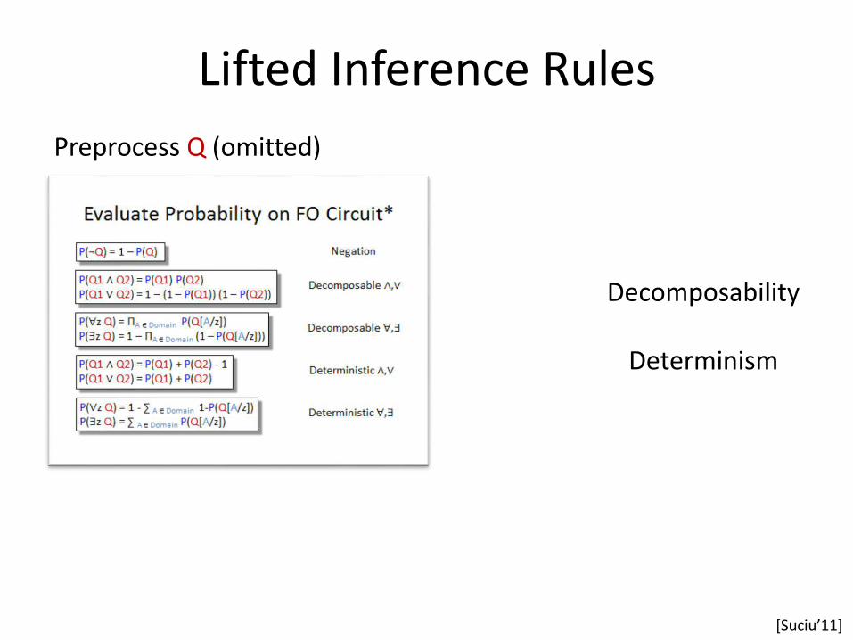
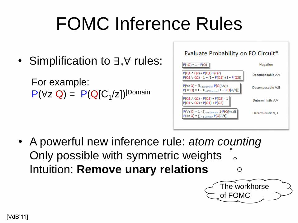
Evaluate Probability on FO Circuit*
* Also non-NNF to simplify examples. Some rules redundant given others.
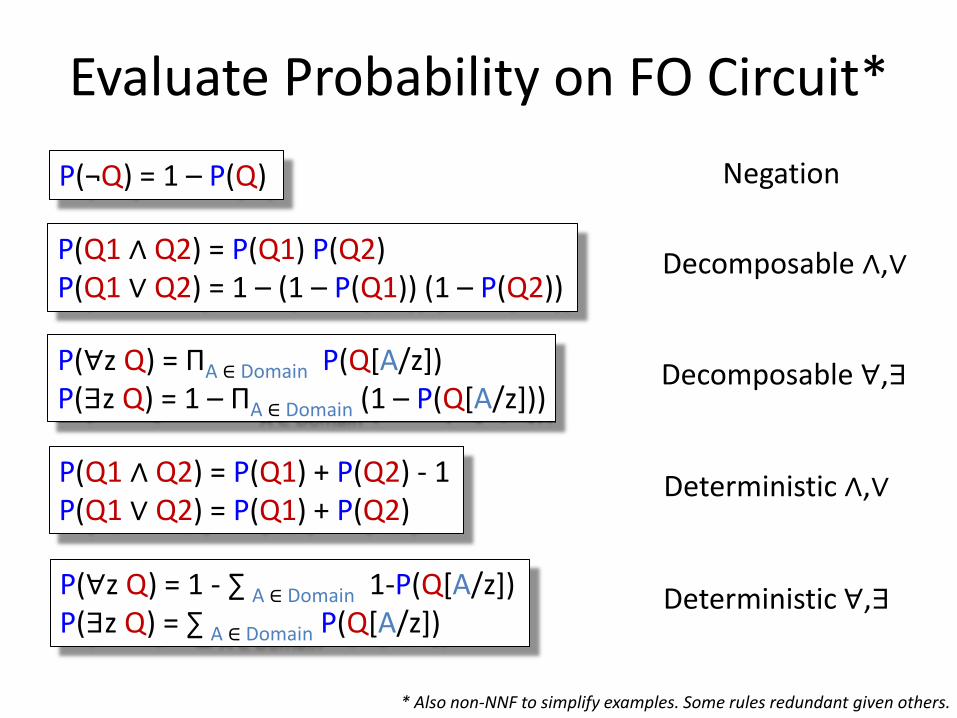
Evaluate Probability on FO Circuit*
P(¬Q) = 1 – P(Q) Negation
* Also non-NNF to simplify examples. Some rules redundant given others.
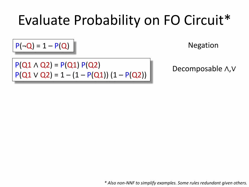
Evaluate Probability on FO Circuit*
P(Q1 ∧ Q2) = P(Q1) P(Q2) P(Q1 ∨ Q2) = 1 – (1 – P(Q1)) (1 – P(Q2))
Decomposable ∧,∨
P(¬Q) = 1 – P(Q) Negation
* Also non-NNF to simplify examples. Some rules redundant given others.
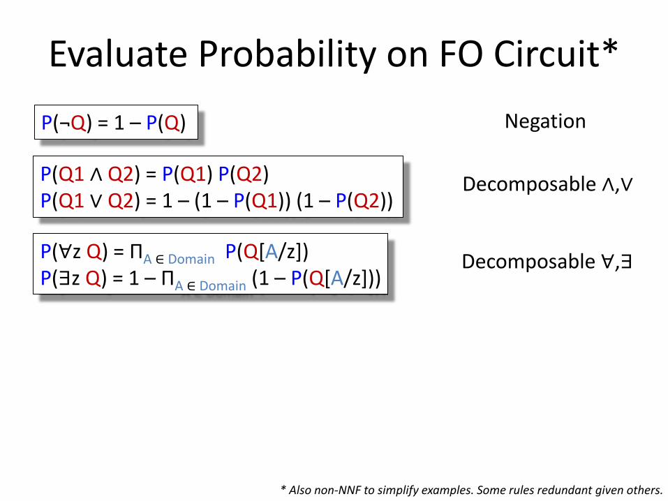
Evaluate Probability on FO Circuit*
P(Q1 ∧ Q2) = P(Q1) P(Q2) P(Q1 ∨ Q2) = 1 – (1 – P(Q1)) (1 – P(Q2))
P(∀z Q) = ΠA ∈ Domain P(Q[A/z]) P(∃z Q) = 1 – ΠA ∈ Domain (1 – P(Q[A/z]))
Decomposable ∧,∨
Decomposable ∀,∃
P(¬Q) = 1 – P(Q) Negation
* Also non-NNF to simplify examples. Some rules redundant given others.
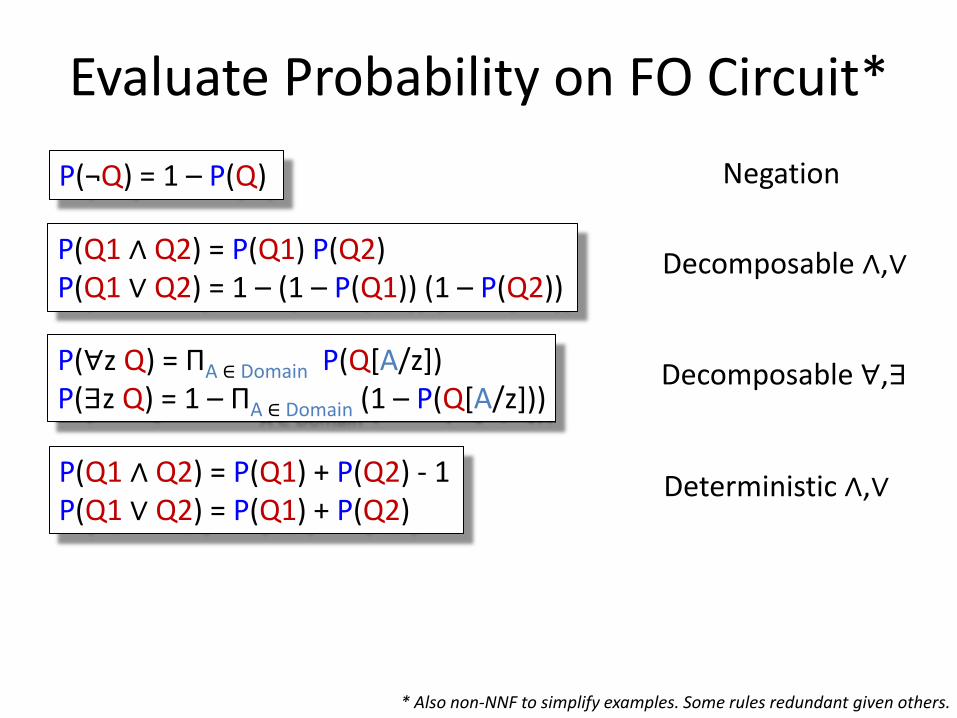
Evaluate Probability on FO Circuit*
P(Q1 ∧ Q2) = P(Q1) P(Q2) P(Q1 ∨ Q2) = 1 – (1 – P(Q1)) (1 – P(Q2))
P(∀z Q) = ΠA ∈ Domain P(Q[A/z]) P(∃z Q) = 1 – ΠA ∈ Domain (1 – P(Q[A/z]))
Decomposable ∧,∨
Decomposable ∀,∃
P(¬Q) = 1 – P(Q) Negation
P(Q1 ∧ Q2) = P(Q1) + P(Q2) - 1 P(Q1 ∨ Q2) = P(Q1) + P(Q2)
Deterministic ∧,∨
* Also non-NNF to simplify examples. Some rules redundant given others.
Evaluate Probability on FO Circuit*
P(Q1 ∧ Q2) = P(Q1) P(Q2) P(Q1 ∨ Q2) = 1 – (1 – P(Q1)) (1 – P(Q2))
P(∀z Q) = ΠA ∈ Domain P(Q[A/z]) P(∃z Q) = 1 – ΠA ∈ Domain (1 – P(Q[A/z]))
Decomposable ∧,∨
Decomposable ∀,∃
P(¬Q) = 1 – P(Q) Negation
P(Q1 ∧ Q2) = P(Q1) + P(Q2) - 1 P(Q1 ∨ Q2) = P(Q1) + P(Q2)
Deterministic ∧,∨
P(∀z Q) = 1 - ∑ A ∈ Domain 1-P(Q[A/z]) P(∃z Q) = ∑ A ∈ Domain P(Q[A/z])
Deterministic ∀,∃
* Also non-NNF to simplify examples. Some rules redundant given others.
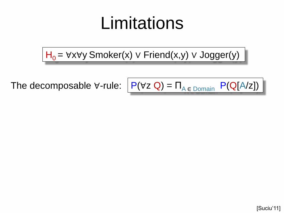
Limitations
H0 = ∀x∀y Smoker(x) ∨ Friend(x,y) ∨ Jogger(y)
The decomposable ∀-rule:
P(∀z Q) = ΠA ∈ Domain P(Q[A/z])
[Suciu‟11]
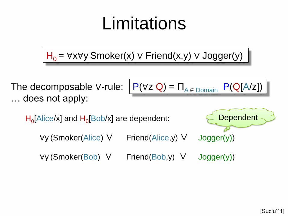
Limitations
H0 = ∀x∀y Smoker(x) ∨ Friend(x,y) ∨ Jogger(y)
The decomposable ∀-rule:
… does not apply:
H0[Alice/x] and H0[Bob/x] are dependent:
∀y (Smoker(Alice) ∨ Friend(Alice,y) ∨ Jogger(y))
∀y (Smoker(Bob) ∨ Friend(Bob,y) ∨ Jogger(y))
Dependent
P(∀z Q) = ΠA ∈ Domain P(Q[A/z])
[Suciu‟11]
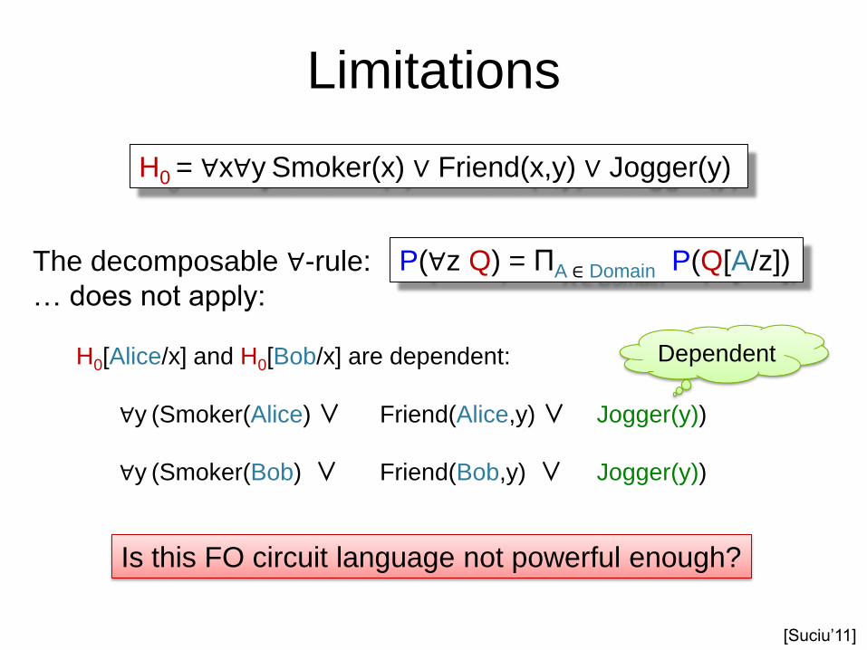
Limitations
H0 = ∀x∀y Smoker(x) ∨ Friend(x,y) ∨ Jogger(y)
The decomposable ∀-rule:
… does not apply:
H0[Alice/x] and H0[Bob/x] are dependent:
∀y (Smoker(Alice) ∨ Friend(Alice,y) ∨ Jogger(y))
∀y (Smoker(Bob) ∨ Friend(Bob,y) ∨ Jogger(y))
Dependent
Is this FO circuit language not powerful enough?
P(∀z Q) = ΠA ∈ Domain P(Q[A/z])
[Suciu‟11]
Background:
Positive Partitioned 2CNF
1
2
1
2
3
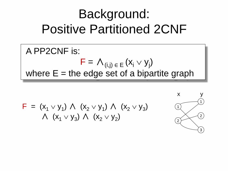
A PP2CNF is:
F = ∧(i,j) ∈ E (xi yj)
where E = the edge set of a bipartite graph
F = (x1 y1) ∧ (x2 y1) ∧ (x2 y3)
∧ (x1 y3) ∧ (x2 y2)
x y
Background:
Positive Partitioned 2CNF
1
2
1
2
3
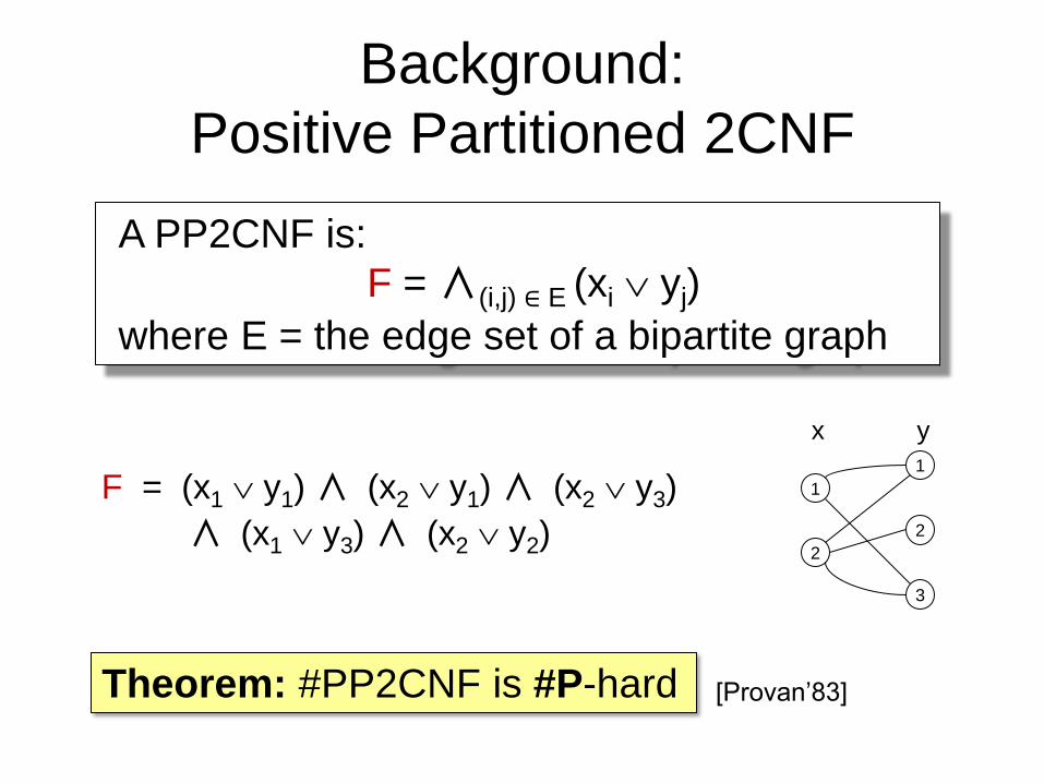
A PP2CNF is:
F = ∧(i,j) ∈ E (xi yj)
where E = the edge set of a bipartite graph
F = (x1 y1) ∧ (x2 y1) ∧ (x2 y3)
∧ (x1 y3) ∧ (x2 y2)
x y
Theorem: #PP2CNF is #P-hard [Provan‟83]
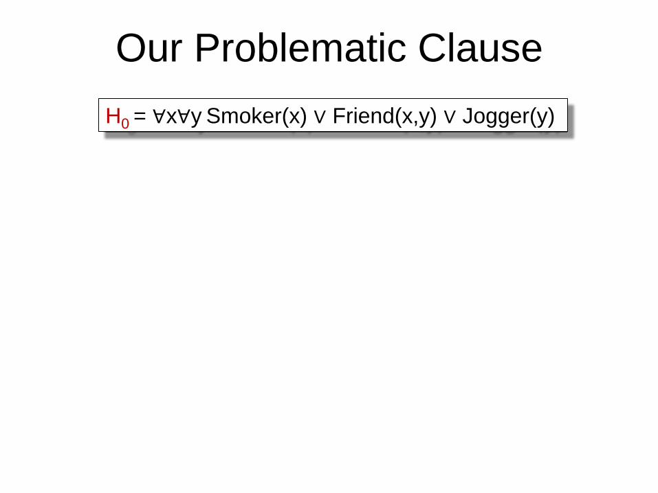
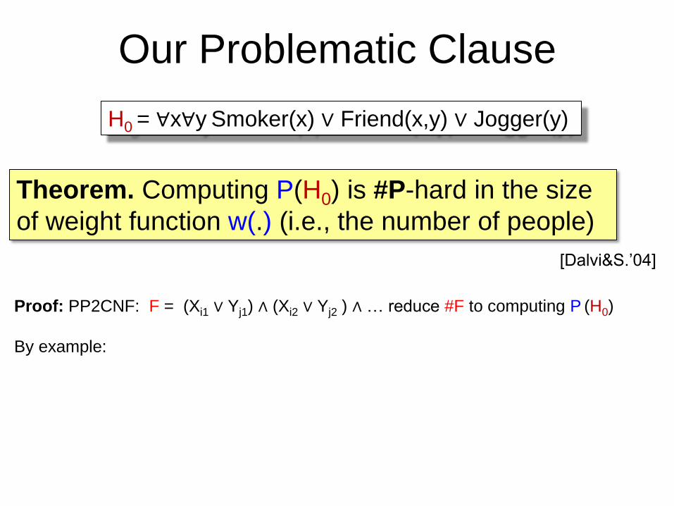
Our Problematic Clause
H0 = ∀x∀y Smoker(x) ∨ Friend(x,y) ∨ Jogger(y)
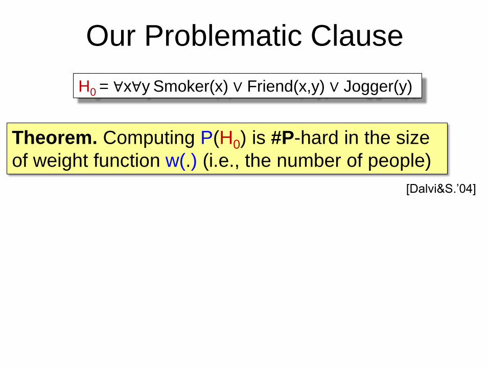
Our Problematic Clause
Theorem. Computing P(H0) is #P-hard in the size
of weight function w(.) (i.e., the number of people)
[Dalvi&S.‟04]
H0 = ∀x∀y Smoker(x) ∨ Friend(x,y) ∨ Jogger(y)
Our Problematic Clause
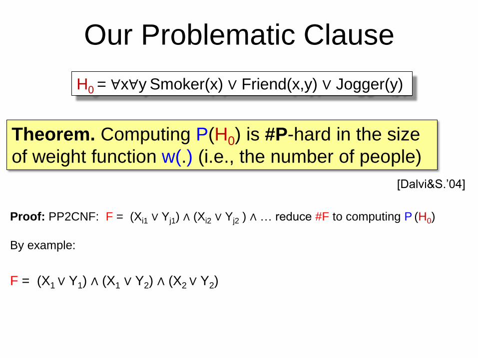
Proof: PP2CNF: F = (Xi1 ∨ Yj1) ∧ (Xi2 ∨ Yj2 ) ∧ … reduce #F to computing P (H0)
By example:
Theorem. Computing P(H0) is #P-hard in the size
of weight function w(.) (i.e., the number of people)
[Dalvi&S.‟04]
H0 = ∀x∀y Smoker(x) ∨ Friend(x,y) ∨ Jogger(y)
Our Problematic Clause
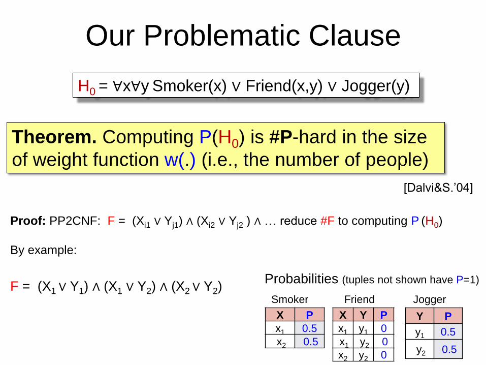
Proof: PP2CNF: F = (Xi1 ∨ Yj1) ∧ (Xi2 ∨ Yj2 ) ∧ … reduce #F to computing P (H0)
By example:
F = (X1 ∨ Y1) ∧ (X1 ∨ Y2) ∧ (X2 ∨ Y2)
Theorem. Computing P(H0) is #P-hard in the size
of weight function w(.) (i.e., the number of people)
[Dalvi&S.‟04]
H0 = ∀x∀y Smoker(x) ∨ Friend(x,y) ∨ Jogger(y)
Our Problematic Clause
Proof: PP2CNF: F = (Xi1 ∨ Yj1) ∧ (Xi2 ∨ Yj2 ) ∧ … reduce #F to computing P (H0)
By example:
X Y P
x1 y1 0
x1 y2 0
x2 y2 0
X P
x1 0.5
x2 0.5
Y P
y1 0.5
y2 0.5
Smoker Jogger Friend F = (X1 ∨ Y1) ∧ (X1 ∨ Y2) ∧ (X2 ∨ Y2)
Theorem. Computing P(H0) is #P-hard in the size
of weight function w(.) (i.e., the number of people)
[Dalvi&S.‟04]
Probabilities (tuples not shown have P=1)
H0 = ∀x∀y Smoker(x) ∨ Friend(x,y) ∨ Jogger(y)
Our Problematic Clause
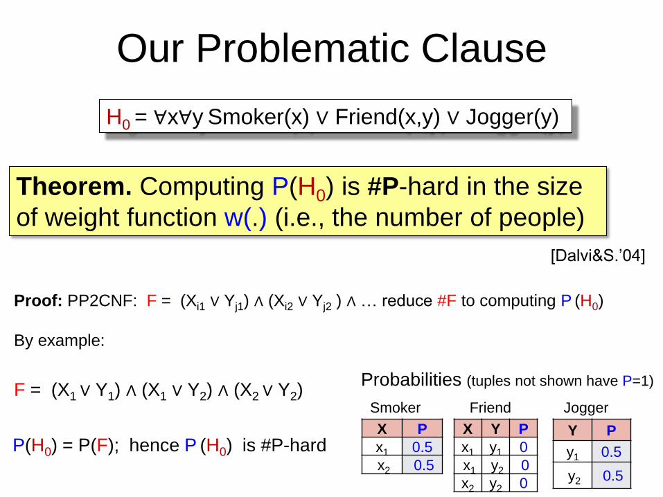
Proof: PP2CNF: F = (Xi1 ∨ Yj1) ∧ (Xi2 ∨ Yj2 ) ∧ … reduce #F to computing P (H0)
By example:
X Y P
x1 y1 0
x1 y2 0
x2 y2 0
X P
x1 0.5
x2 0.5
Y P
y1 0.5
y2 0.5
Smoker Jogger Friend
P(H0) = P(F); hence P (H0) is #P-hard
F = (X1 ∨ Y1) ∧ (X1 ∨ Y2) ∧ (X2 ∨ Y2)
Theorem. Computing P(H0) is #P-hard in the size
of weight function w(.) (i.e., the number of people)
[Dalvi&S.‟04]
Probabilities (tuples not shown have P=1)
H0 = ∀x∀y Smoker(x) ∨ Friend(x,y) ∨ Jogger(y)

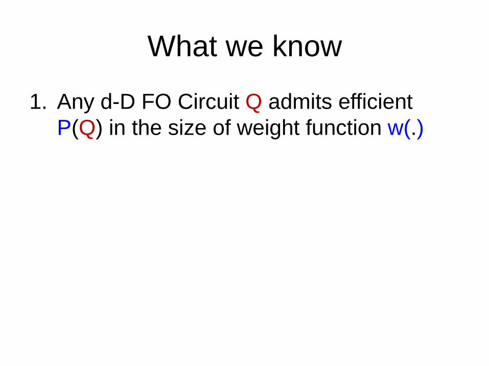
What we know
What we know
1. Any d-D FO Circuit Q admits efficient
P(Q) in the size of weight function w(.)
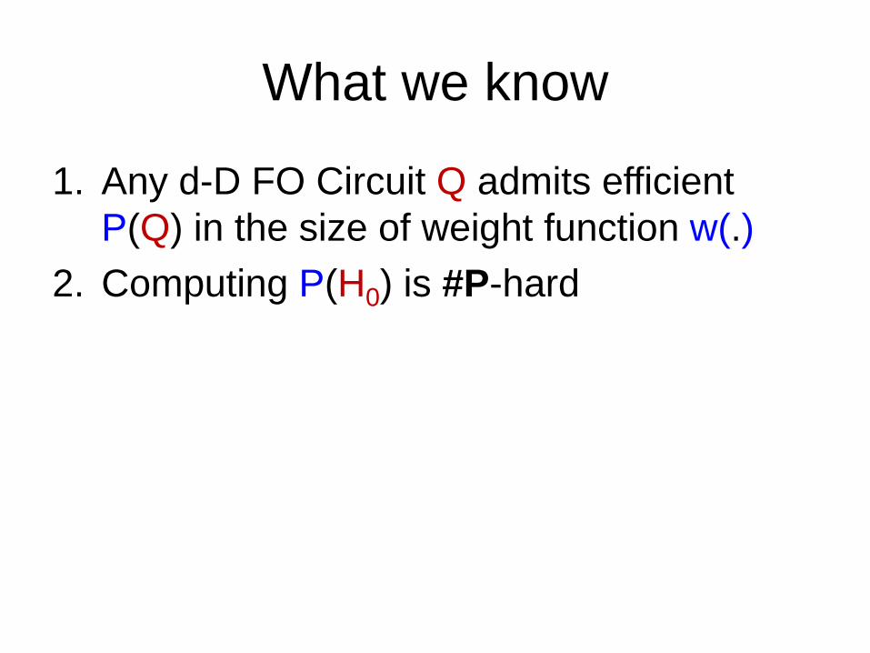
What we know
1. Any d-D FO Circuit Q admits efficient
P(Q) in the size of weight function w(.)
2. Computing P(H0) is #P-hard
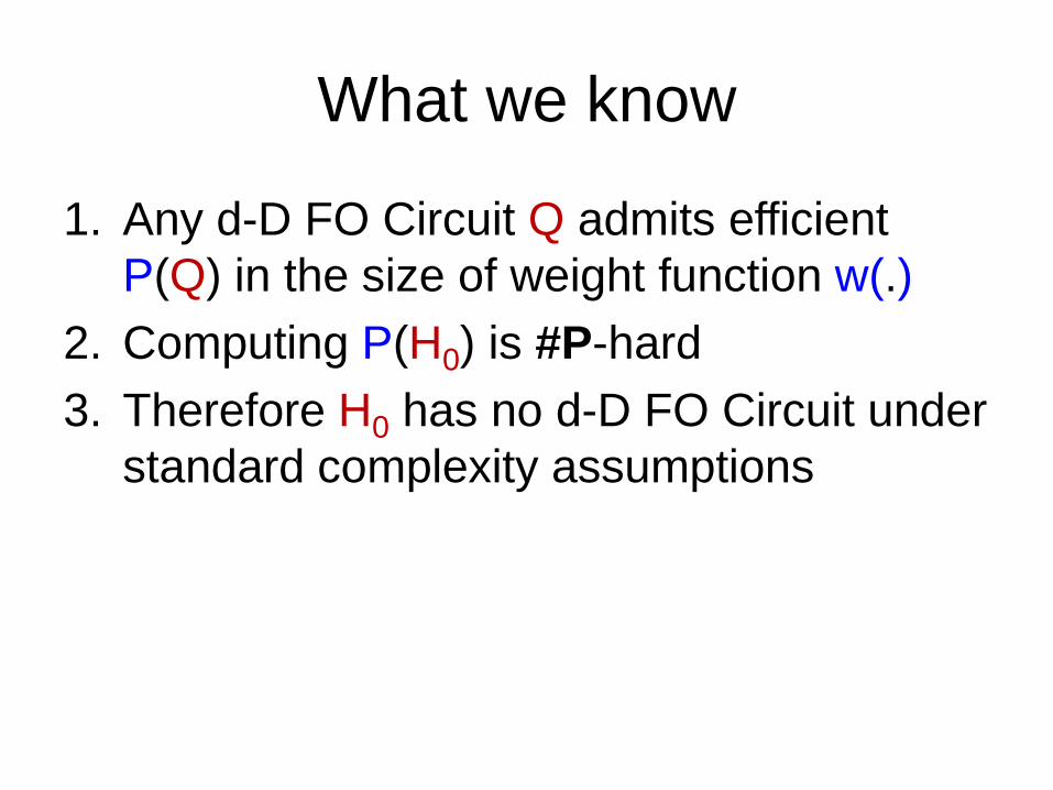
What we know
1. Any d-D FO Circuit Q admits efficient
P(Q) in the size of weight function w(.)
2. Computing P(H0) is #P-hard
3. Therefore H0 has no d-D FO Circuit under
standard complexity assumptions
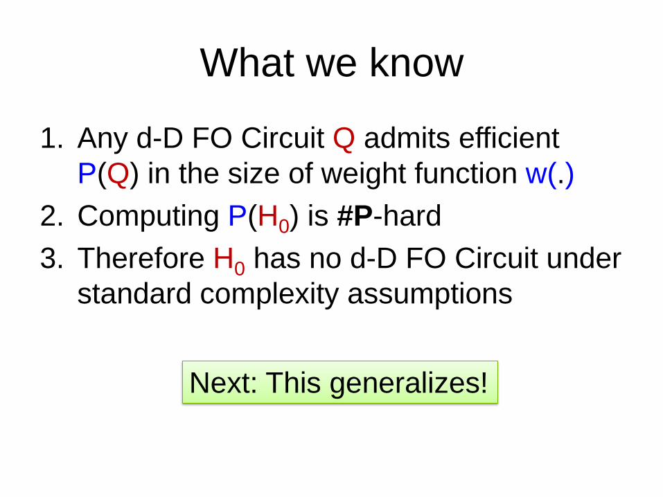
What we know
1. Any d-D FO Circuit Q admits efficient
P(Q) in the size of weight function w(.)
2. Computing P(H0) is #P-hard
3. Therefore H0 has no d-D FO Circuit under
standard complexity assumptions
Next: This generalizes!
Background: Hierarchical Queries
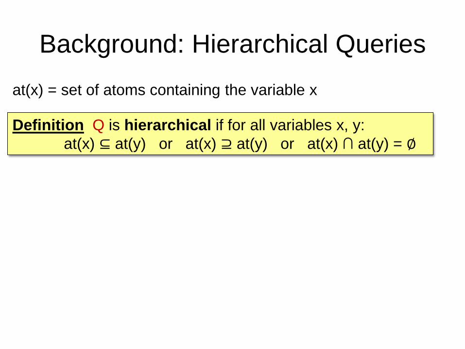
at(x) = set of atoms containing the variable x
Definition Q is hierarchical if for all variables x, y:
at(x) ⊆ at(y) or at(x) ⊇ at(y) or at(x) ∩ at(y) = ∅
Background: Hierarchical Queries
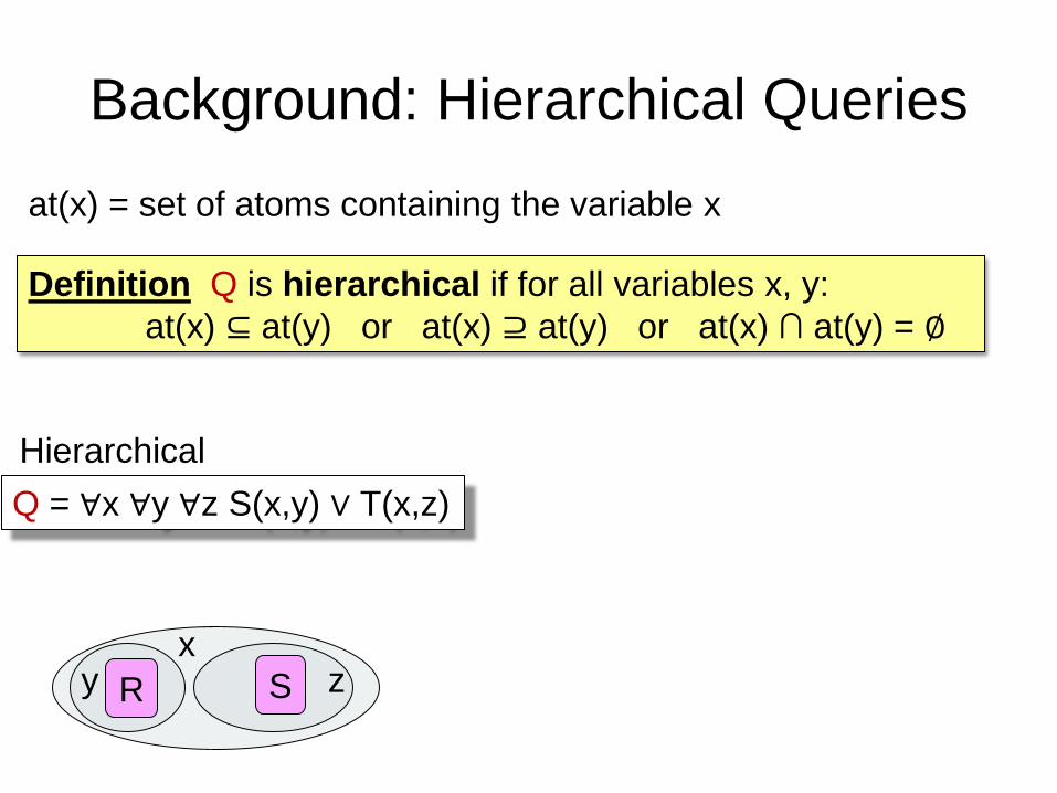
at(x) = set of atoms containing the variable x
R S
x z
Hierarchical
y
Q = ∀x ∀y ∀z S(x,y) ∨ T(x,z)
Definition Q is hierarchical if for all variables x, y:
at(x) ⊆ at(y) or at(x) ⊇ at(y) or at(x) ∩ at(y) = ∅

Background: Hierarchical Queries
at(x) = set of atoms containing the variable x
S F x y
J
Non-hierarchical
R S
x z
Hierarchical
y
Q = ∀x ∀y ∀z S(x,y) ∨ T(x,z) H0 = ∀x ∀y S(x) ∨ F(x,y) ∨ J(y)
Definition Q is hierarchical if for all variables x, y:
at(x) ⊆ at(y) or at(x) ⊇ at(y) or at(x) ∩ at(y) = ∅
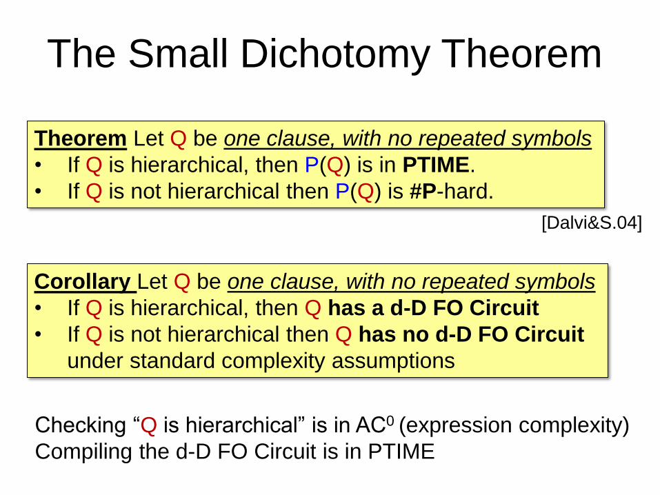
The Small Dichotomy Theorem
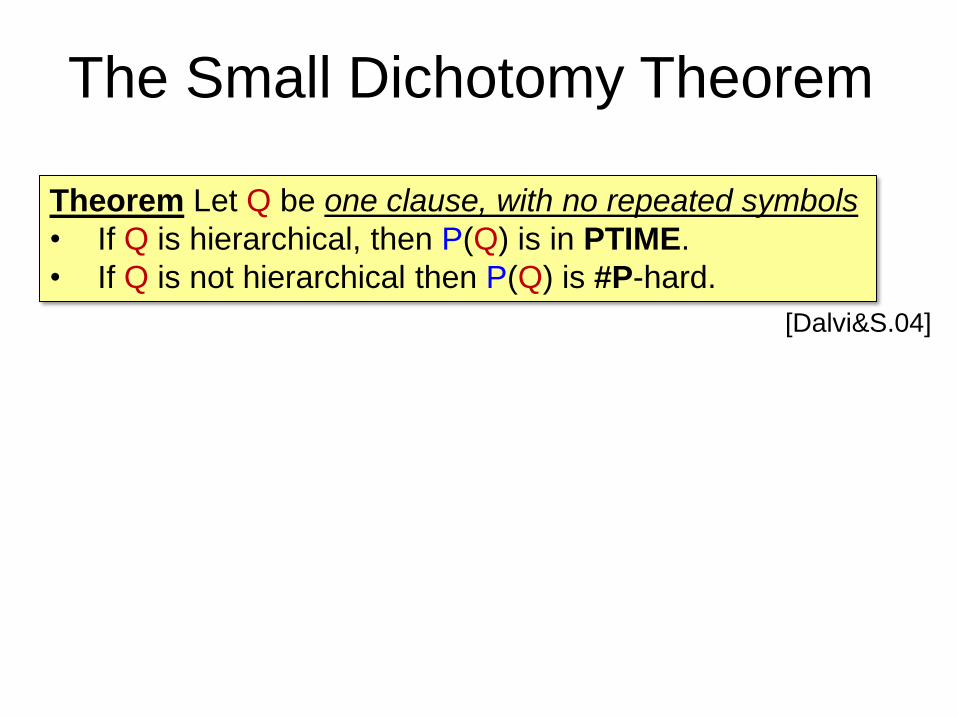
Theorem Let Q be one clause, with no repeated symbols
• If Q is hierarchical, then P(Q) is in PTIME.
• If Q is not hierarchical then P(Q) is #P-hard.
[Dalvi&S.04]
The Small Dichotomy Theorem
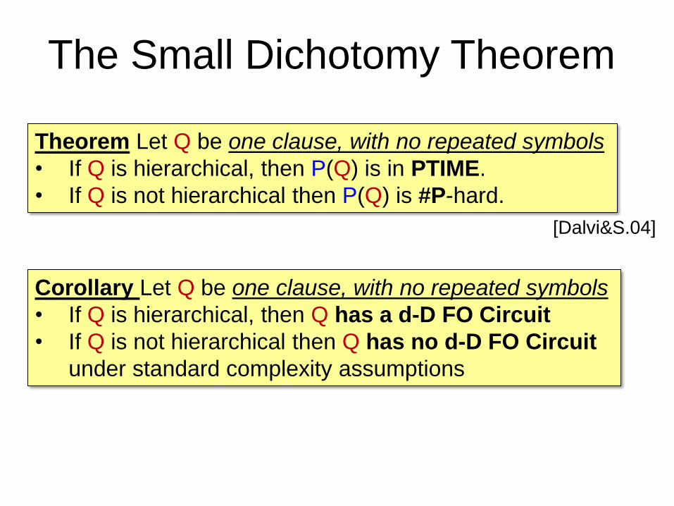
Theorem Let Q be one clause, with no repeated symbols
• If Q is hierarchical, then P(Q) is in PTIME.
• If Q is not hierarchical then P(Q) is #P-hard.
[Dalvi&S.04]
Corollary Let Q be one clause, with no repeated symbols
• If Q is hierarchical, then Q has a d-D FO Circuit
• If Q is not hierarchical then Q has no d-D FO Circuit
under standard complexity assumptions
The Small Dichotomy Theorem
Checking “Q is hierarchical” is in AC0 (expression complexity)
Compiling the d-D FO Circuit is in PTIME
Theorem Let Q be one clause, with no repeated symbols
• If Q is hierarchical, then P(Q) is in PTIME.
• If Q is not hierarchical then P(Q) is #P-hard.
[Dalvi&S.04]
Corollary Let Q be one clause, with no repeated symbols
• If Q is hierarchical, then Q has a d-D FO Circuit
• If Q is not hierarchical then Q has no d-D FO Circuit
under standard complexity assumptions
Proof
Hierarchical PTIME
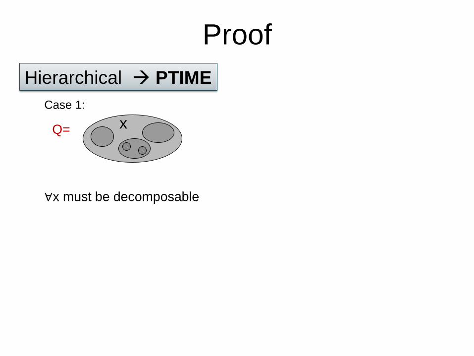
Proof
Hierarchical PTIME
∀x must be decomposable
x
Case 1:
Q=
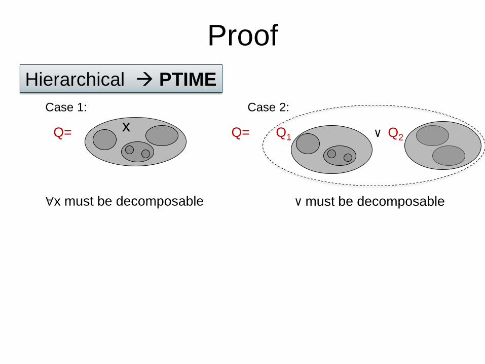
Proof
Hierarchical PTIME
∀x must be decomposable
x
Case 1:
Q= Q1 v Q2 Q=
Case 2:
v must be decomposable
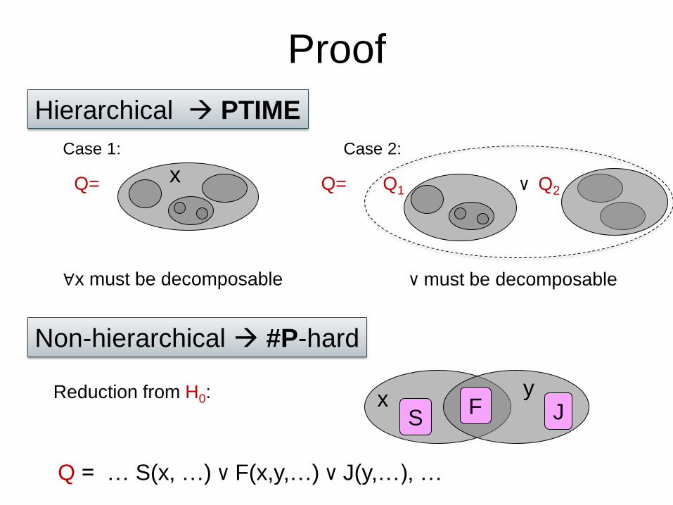
Proof
Hierarchical PTIME
Non-hierarchical #P-hard
Reduction from H0:
Q = … S(x, …) v F(x,y,…) v J(y,…), …
x y
S F J
∀x must be decomposable
x
Case 1:
Q= Q1 v Q2 Q=
Case 2:
v must be decomposable
Overview
1. Propositional Refresher
2. Primer: A First-Order Tractable Language
3. Probabilistic Databases
4. Symmetric First-Order Model Counting
5. Lots of Pointers
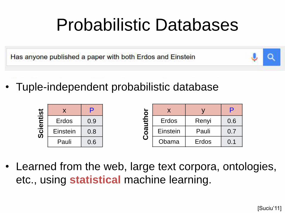
• Tuple-independent probabilistic database
• Learned from the web, large text corpora, ontologies,
etc., using statistical machine learning.
Co
au
tho
r
Probabilistic Databases
x y P
Erdos Renyi 0.6
Einstein Pauli 0.7
Obama Erdos 0.1
Scie
nti
st x P
Erdos 0.9
Einstein 0.8
Pauli 0.6
[Suciu‟11]
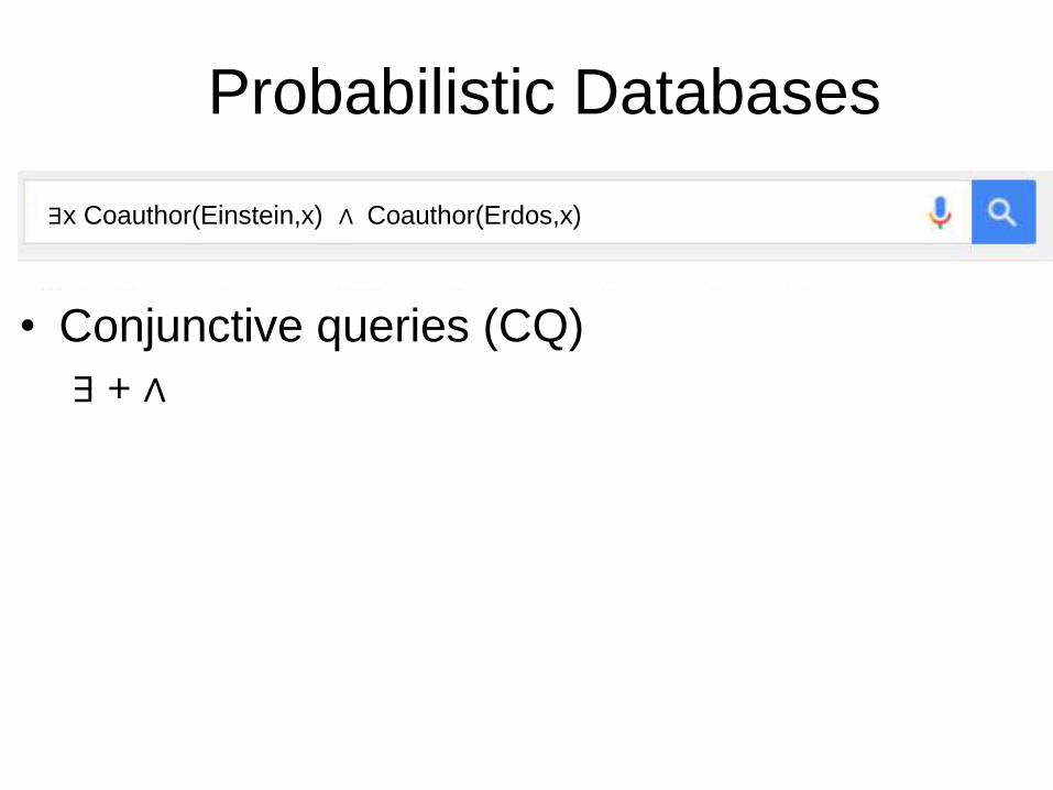
• Conjunctive queries (CQ)
∃ + ∧
Probabilistic Databases
∃x Coauthor(Einstein,x) ∧ Coauthor(Erdos,x)
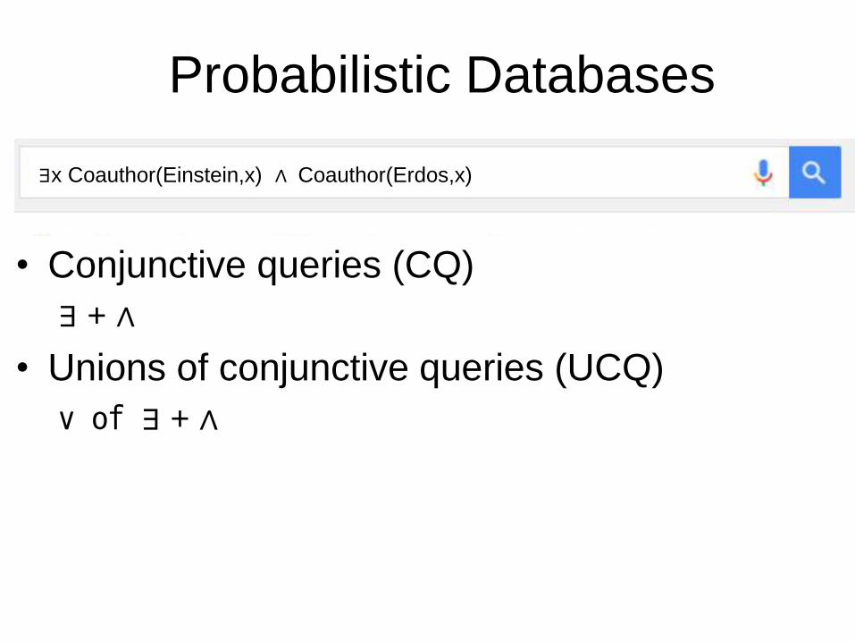
• Conjunctive queries (CQ)
∃ + ∧
• Unions of conjunctive queries (UCQ)
v of ∃ + ∧
Probabilistic Databases
∃x Coauthor(Einstein,x) ∧ Coauthor(Erdos,x)
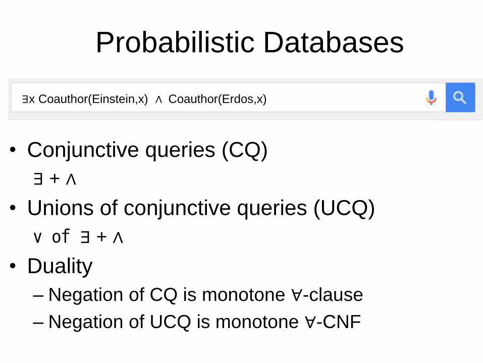
• Conjunctive queries (CQ)
∃ + ∧
• Unions of conjunctive queries (UCQ)
v of ∃ + ∧
• Duality
– Negation of CQ is monotone ∀-clause
– Negation of UCQ is monotone ∀-CNF
Probabilistic Databases
∃x Coauthor(Einstein,x) ∧ Coauthor(Erdos,x)
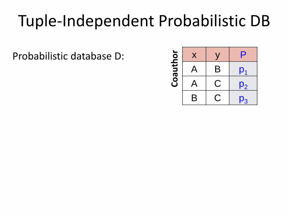
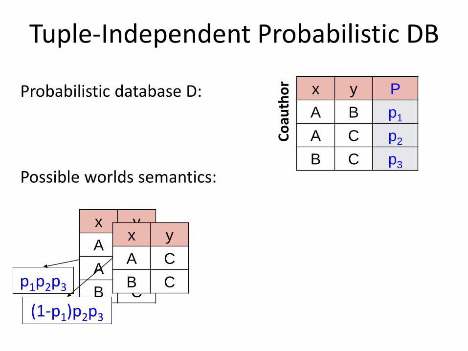
Tuple-Independent Probabilistic DB
x y P
A B p1
A C p2
B C p3
Probabilistic database D:
Co
auth
or
x y
A B
A C
B C
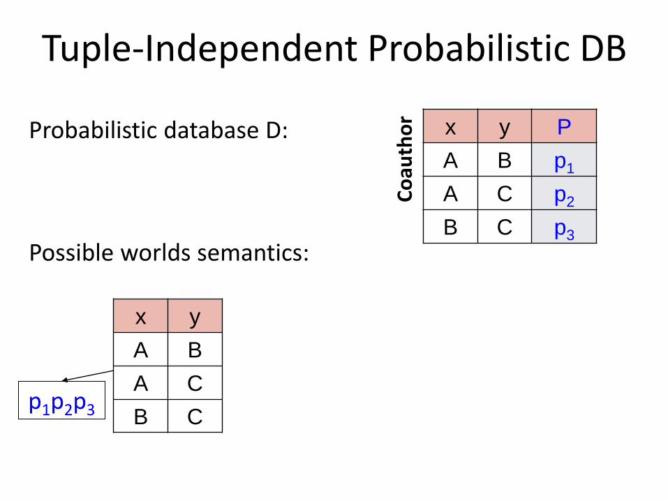
Tuple-Independent Probabilistic DB
x y P
A B p1
A C p2
B C p3
Possible worlds semantics:
p1p2p3
Probabilistic database D:
Co
auth
or
x y
A B
A C
B C
Tuple-Independent Probabilistic DB
x y P
A B p1
A C p2
B C p3
Possible worlds semantics:
p1p2p3
(1-p1)p2p3
Probabilistic database D:
x y
A C
B C C
oau
tho
r
x y
A B
A C
B C
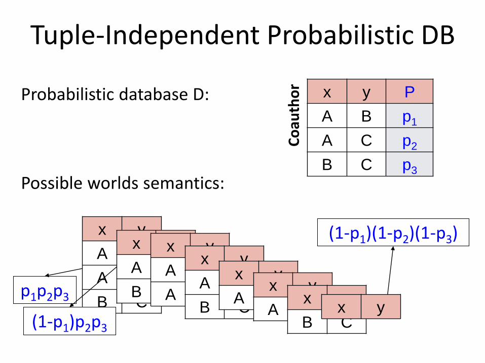
Tuple-Independent Probabilistic DB
x y P
A B p1
A C p2
B C p3
Possible worlds semantics:
p1p2p3
(1-p1)p2p3
(1-p1)(1-p2)(1-p3)
Probabilistic database D:
x y
A C
B C
x y
A B
A C
x y
A B
B C
x y
A B x y
A C x y
B C x y
Co
auth
or
x y P
A D q1 Y1
A E q2 Y2
B F q3 Y3
B G q4 Y4
B H q5 Y5
x P
A p1 X1
B p2 X2
C p3 X3
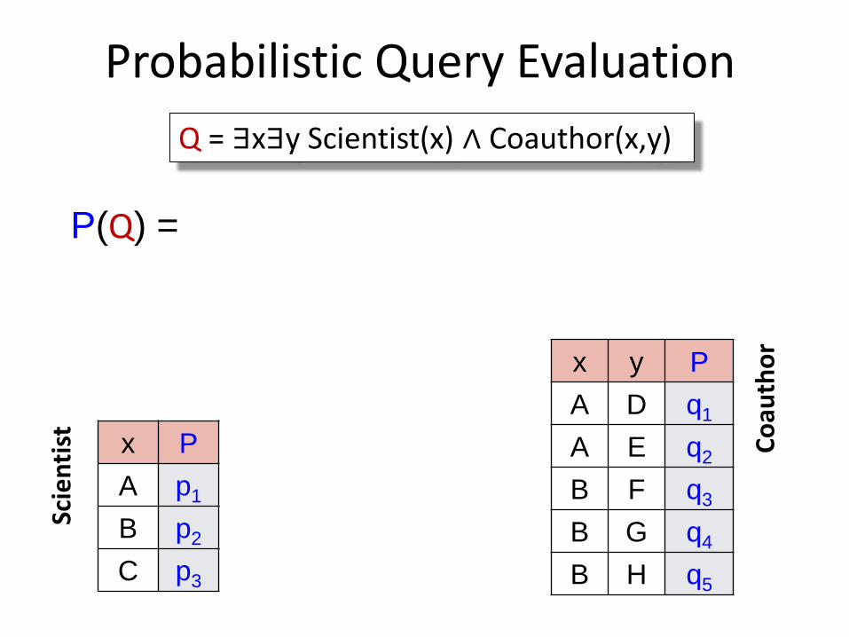
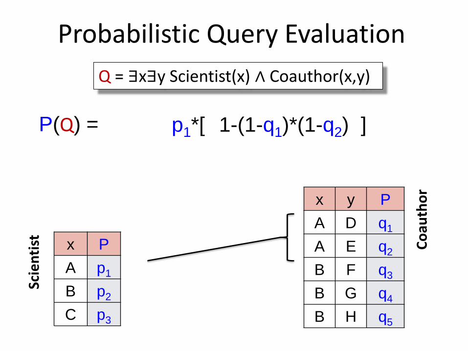
P(Q) =
Probabilistic Query Evaluation
Q = ∃x∃y Scientist(x) ∧ Coauthor(x,y)
Scie
nti
st
Co
auth
or
x y P
A D q1 Y1
A E q2 Y2
B F q3 Y3
B G q4 Y4
B H q5 Y5
x P
A p1 X1
B p2 X2
C p3 X3
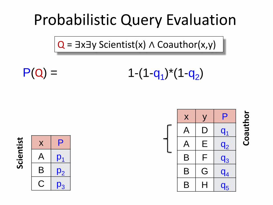
P(Q) = 1-(1-q1)*(1-q2)
Probabilistic Query Evaluation
Q = ∃x∃y Scientist(x) ∧ Coauthor(x,y)
Scie
nti
st
Co
auth
or
x y P
A D q1 Y1
A E q2 Y2
B F q3 Y3
B G q4 Y4
B H q5 Y5
x P
A p1 X1
B p2 X2
C p3 X3
P(Q) = 1-(1-q1)*(1-q2) p1*[ ]
Probabilistic Query Evaluation
Q = ∃x∃y Scientist(x) ∧ Coauthor(x,y)
Scie
nti
st
Co
auth
or
x y P
A D q1 Y1
A E q2 Y2
B F q3 Y3
B G q4 Y4
B H q5 Y5
x P
A p1 X1
B p2 X2
C p3 X3
P(Q) = 1-(1-q1)*(1-q2) p1*[ ]
1-(1-q3)*(1-q4)*(1-q5)
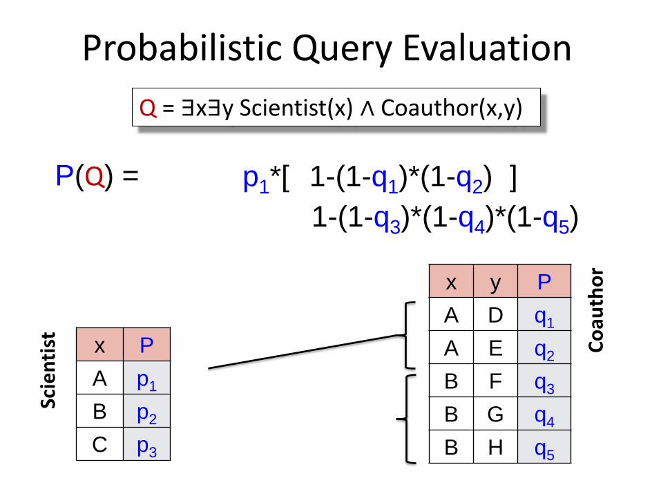
Probabilistic Query Evaluation
Q = ∃x∃y Scientist(x) ∧ Coauthor(x,y)
Scie
nti
st
Co
auth
or
x y P
A D q1 Y1
A E q2 Y2
B F q3 Y3
B G q4 Y4
B H q5 Y5
x P
A p1 X1
B p2 X2
C p3 X3
P(Q) = 1-(1-q1)*(1-q2) p1*[ ]
1-(1-q3)*(1-q4)*(1-q5) p2*[ ]
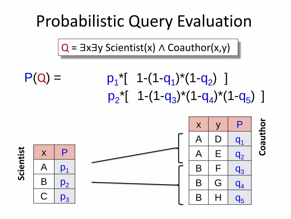
Probabilistic Query Evaluation
Q = ∃x∃y Scientist(x) ∧ Coauthor(x,y)
Scie
nti
st
Co
auth
or
x y P
A D q1 Y1
A E q2 Y2
B F q3 Y3
B G q4 Y4
B H q5 Y5
x P
A p1 X1
B p2 X2
C p3 X3
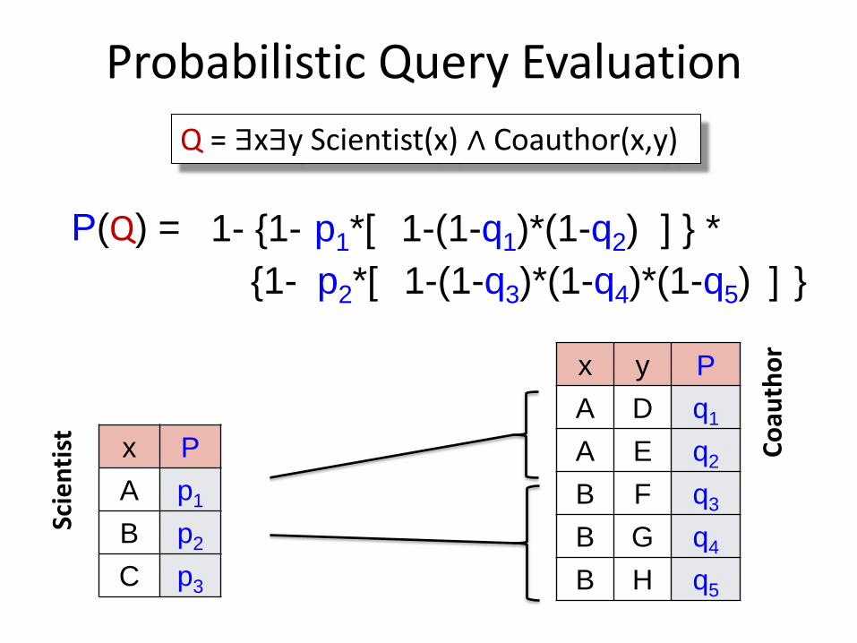
P(Q) = 1-(1-q1)*(1-q2) p1*[ ]
1-(1-q3)*(1-q4)*(1-q5) p2*[ ]
1- {1- } *
{1- }
Probabilistic Query Evaluation
Q = ∃x∃y Scientist(x) ∧ Coauthor(x,y)
Scie
nti
st
Co
auth
or
x y
A B
A C
B C
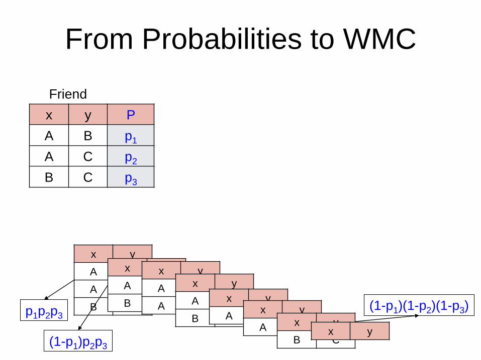
From Probabilities to WMC
Friend
x y P
A B p1
A C p2
B C p3
p1p2p3
(1-p1)p2p3
(1-p1)(1-p2)(1-p3)
x y
A C
B C
x y
A B
A C
x y
A B
B C
x y
A B x y
A C x y
B C x y
x y
A B
A C
B C
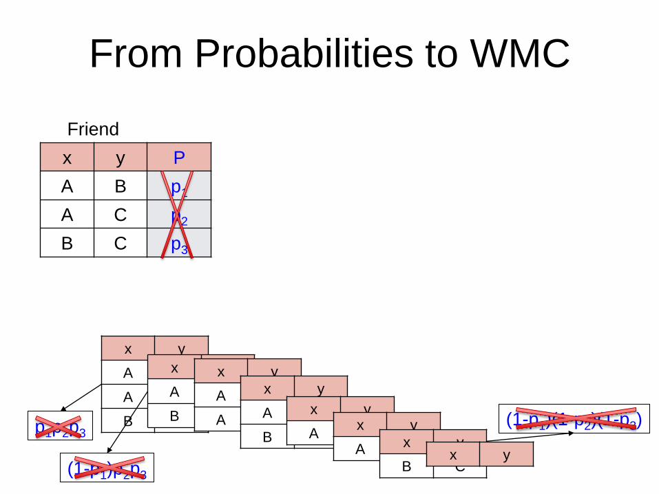
From Probabilities to WMC
Friend
x y P
A B p1
A C p2
B C p3
p1p2p3
(1-p1)p2p3
(1-p1)(1-p2)(1-p3)
x y
A C
B C
x y
A B
A C
x y
A B
B C
x y
A B x y
A C x y
B C x y
x y
A B
A C
B C
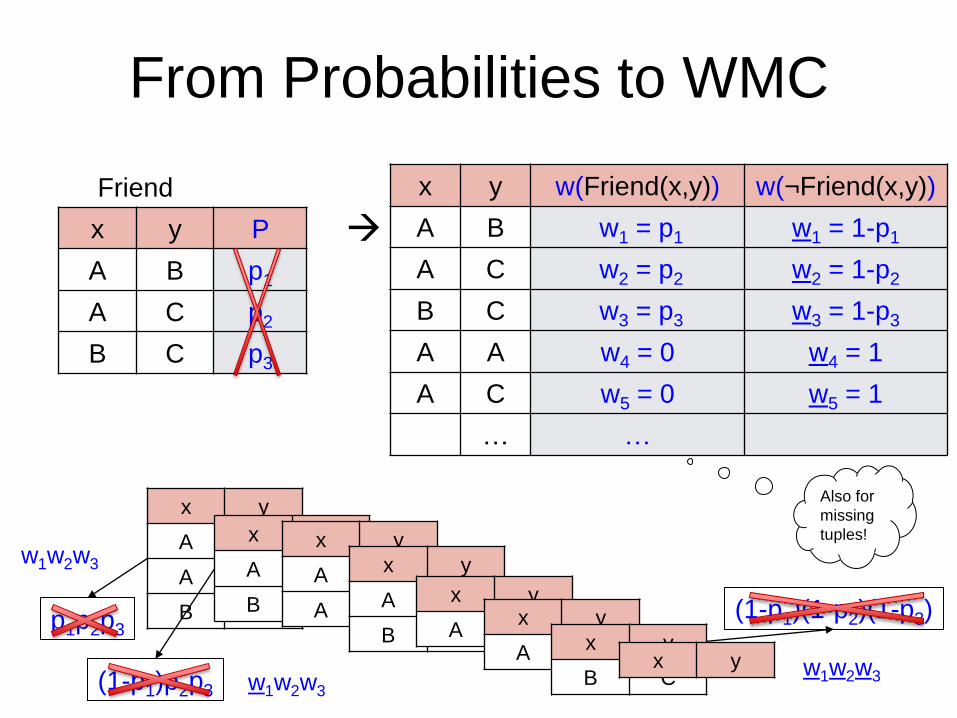
From Probabilities to WMC
Friend
x y P
A B p1
A C p2
B C p3
p1p2p3
(1-p1)p2p3
(1-p1)(1-p2)(1-p3)
x y
A C
B C
x y
A B
A C
x y
A B
B C
x y
A B x y
A C x y
B C x y
x y w(Friend(x,y)) w(¬Friend(x,y))
A B w1 = p1 w1 = 1-p1
A C w2 = p2 w2 = 1-p2
B C w3 = p3 w3 = 1-p3
A A w4 = 0 w4 = 1
A C w5 = 0 w5 = 1
… …
Also for
missing
tuples!
w1w2w3
w1w2w3
w1w2w3
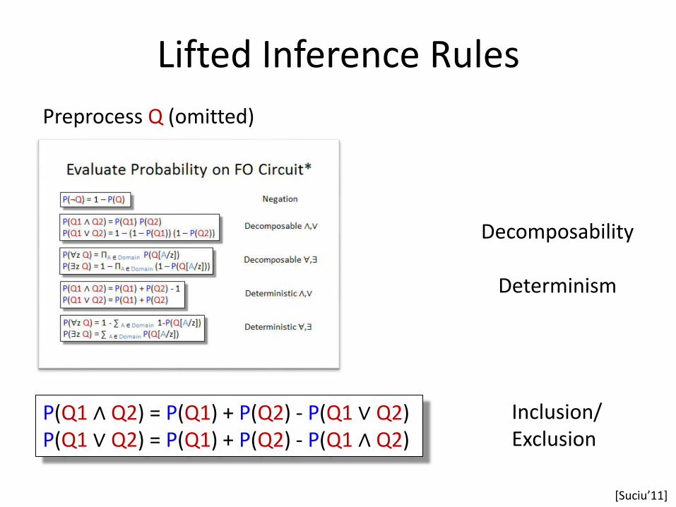
Lifted Inference Rules
Preprocess Q (omitted)
*Suciu’11+
Lifted Inference Rules
Preprocess Q (omitted)
*Suciu’11+
Decomposability
Determinism
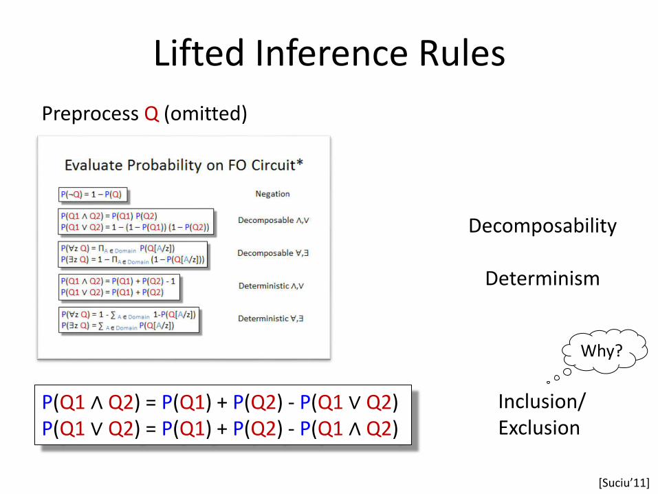
Lifted Inference Rules
P(Q1 ∧ Q2) = P(Q1) + P(Q2) - P(Q1 ∨ Q2) P(Q1 ∨ Q2) = P(Q1) + P(Q2) - P(Q1 ∧ Q2)
Preprocess Q (omitted)
Inclusion/ Exclusion
*Suciu’11+
Decomposability
Determinism
Lifted Inference Rules
P(Q1 ∧ Q2) = P(Q1) + P(Q2) - P(Q1 ∨ Q2) P(Q1 ∨ Q2) = P(Q1) + P(Q2) - P(Q1 ∧ Q2)
Preprocess Q (omitted)
Inclusion/ Exclusion
*Suciu’11+
Decomposability
Determinism
Why?
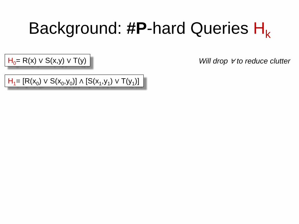
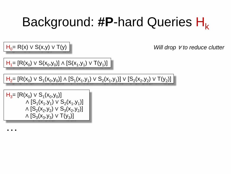
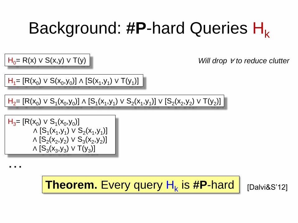
Background: #P-hard Queries Hk
H0= R(x) ∨ S(x,y) ∨ T(y) Will drop ∀ to reduce clutter
H1= [R(x0) ∨ S(x0,y0)] ∧ [S(x1,y1) ∨ T(y1)]

Background: #P-hard Queries Hk
H0= R(x) ∨ S(x,y) ∨ T(y)
H2= [R(x0) ∨ S1(x0,y0)] ∧ [S1(x1,y1) ∨ S2(x1,y1)] ∨ [S2(x2,y2) ∨ T(y2)]
Will drop ∀ to reduce clutter
H1= [R(x0) ∨ S(x0,y0)] ∧ [S(x1,y1) ∨ T(y1)]
Background: #P-hard Queries Hk
H0= R(x) ∨ S(x,y) ∨ T(y)
H2= [R(x0) ∨ S1(x0,y0)] ∧ [S1(x1,y1) ∨ S2(x1,y1)] ∨ [S2(x2,y2) ∨ T(y2)]
Will drop ∀ to reduce clutter
H1= [R(x0) ∨ S(x0,y0)] ∧ [S(x1,y1) ∨ T(y1)]
…
H3= [R(x0) ∨ S1(x0,y0)]
∧ [S1(x1,y1) ∨ S2(x1,y1)]
∧ [S2(x2,y2) ∨ S3(x2,y2)]
∧ [S3(x3,y3) ∨ T(y3)]
Theorem. Every query Hk is #P-hard [Dalvi&S‟12]
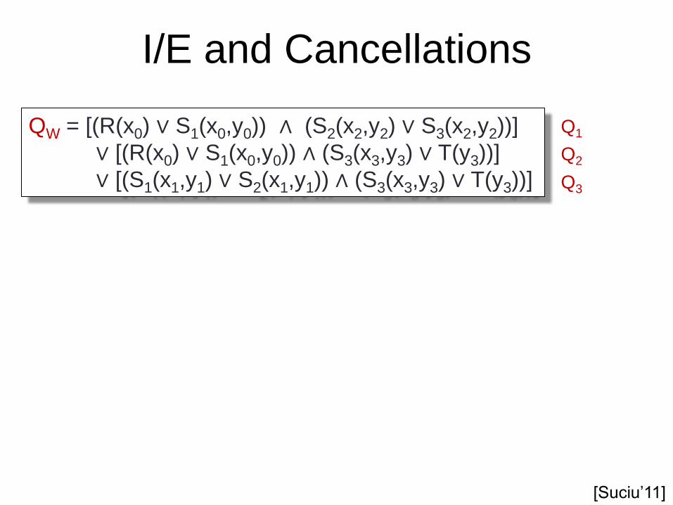
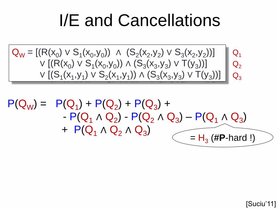
I/E and Cancellations
QW = [(R(x0) ∨ S1(x0,y0)) ∧ (S2(x2,y2) ∨ S3(x2,y2))]
∨ [(R(x0) ∨ S1(x0,y0)) ∧ (S3(x3,y3) ∨ T(y3))]
∨ [(S1(x1,y1) ∨ S2(x1,y1)) ∧ (S3(x3,y3) ∨ T(y3))]
Q1
Q2
Q3
[Suciu‟11]
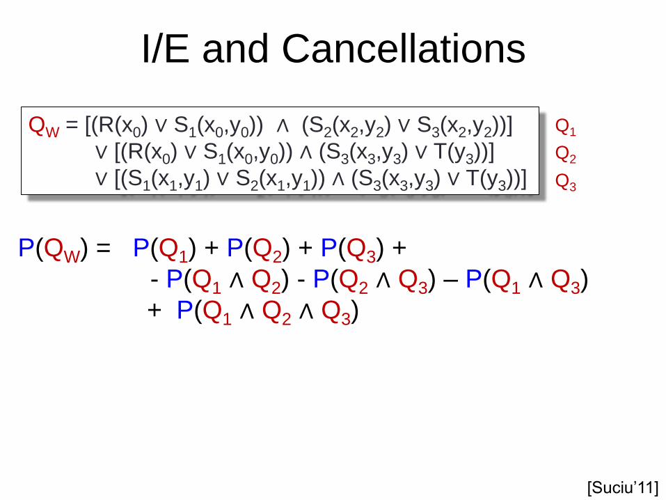
I/E and Cancellations
P(QW) = P(Q1) + P(Q2) + P(Q3) +
- P(Q1 ∧ Q2) - P(Q2 ∧ Q3) – P(Q1 ∧ Q3)
+ P(Q1 ∧ Q2 ∧ Q3)
QW = [(R(x0) ∨ S1(x0,y0)) ∧ (S2(x2,y2) ∨ S3(x2,y2))]
∨ [(R(x0) ∨ S1(x0,y0)) ∧ (S3(x3,y3) ∨ T(y3))]
∨ [(S1(x1,y1) ∨ S2(x1,y1)) ∧ (S3(x3,y3) ∨ T(y3))]
Q1
Q2
Q3
[Suciu‟11]
I/E and Cancellations
P(QW) = P(Q1) + P(Q2) + P(Q3) +
- P(Q1 ∧ Q2) - P(Q2 ∧ Q3) – P(Q1 ∧ Q3)
+ P(Q1 ∧ Q2 ∧ Q3) = H3 (#P-hard !)
QW = [(R(x0) ∨ S1(x0,y0)) ∧ (S2(x2,y2) ∨ S3(x2,y2))]
∨ [(R(x0) ∨ S1(x0,y0)) ∧ (S3(x3,y3) ∨ T(y3))]
∨ [(S1(x1,y1) ∨ S2(x1,y1)) ∧ (S3(x3,y3) ∨ T(y3))]
Q1
Q2
Q3
[Suciu‟11]
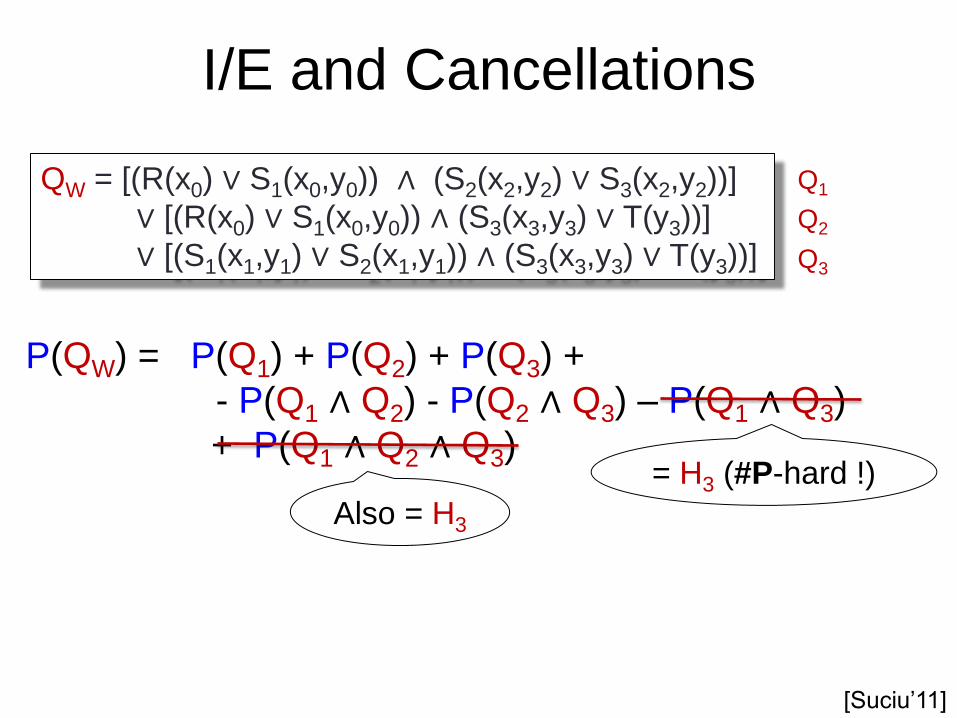
I/E and Cancellations
P(QW) = P(Q1) + P(Q2) + P(Q3) +
- P(Q1 ∧ Q2) - P(Q2 ∧ Q3) – P(Q1 ∧ Q3)
+ P(Q1 ∧ Q2 ∧ Q3)
Also = H3
= H3 (#P-hard !)
QW = [(R(x0) ∨ S1(x0,y0)) ∧ (S2(x2,y2) ∨ S3(x2,y2))]
∨ [(R(x0) ∨ S1(x0,y0)) ∧ (S3(x3,y3) ∨ T(y3))]
∨ [(S1(x1,y1) ∨ S2(x1,y1)) ∧ (S3(x3,y3) ∨ T(y3))]
Q1
Q2
Q3
[Suciu‟11]
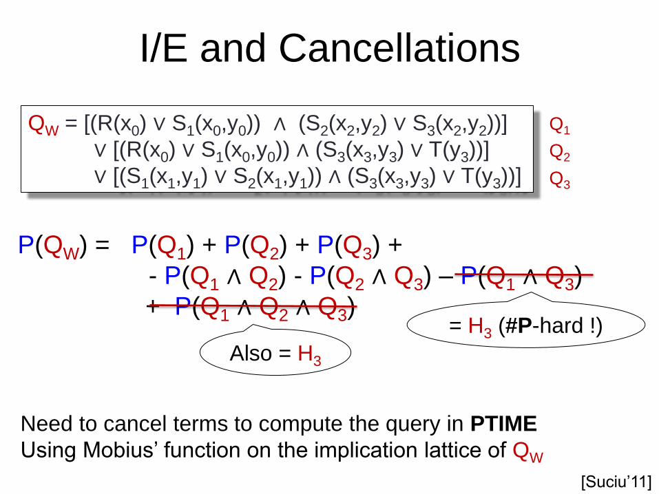
I/E and Cancellations
P(QW) = P(Q1) + P(Q2) + P(Q3) +
- P(Q1 ∧ Q2) - P(Q2 ∧ Q3) – P(Q1 ∧ Q3)
+ P(Q1 ∧ Q2 ∧ Q3)
Also = H3
= H3 (#P-hard !)
QW = [(R(x0) ∨ S1(x0,y0)) ∧ (S2(x2,y2) ∨ S3(x2,y2))]
∨ [(R(x0) ∨ S1(x0,y0)) ∧ (S3(x3,y3) ∨ T(y3))]
∨ [(S1(x1,y1) ∨ S2(x1,y1)) ∧ (S3(x3,y3) ∨ T(y3))]
Need to cancel terms to compute the query in PTIME
Using Mobius‟ function on the implication lattice of QW
Q1
Q2
Q3
[Suciu‟11]
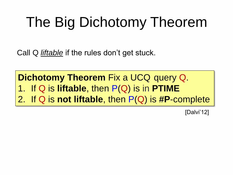
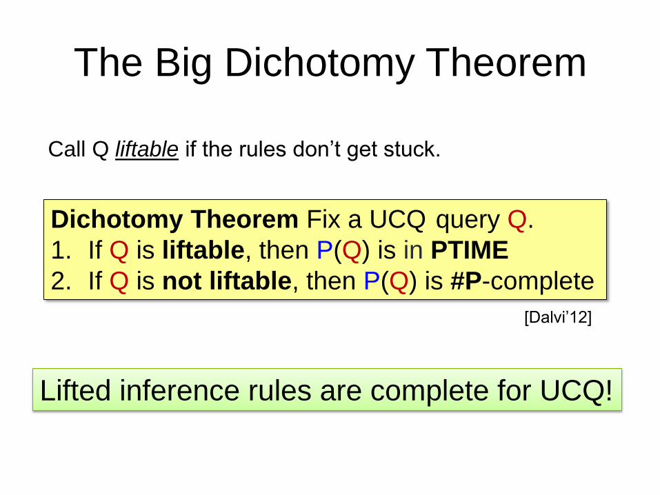
The Big Dichotomy Theorem
Dichotomy Theorem Fix a UCQ query Q.
1. If Q is liftable, then P(Q) is in PTIME
2. If Q is not liftable, then P(Q) is #P-complete
Call Q liftable if the rules don‟t get stuck.
[Dalvi‟12]
The Big Dichotomy Theorem
Dichotomy Theorem Fix a UCQ query Q.
1. If Q is liftable, then P(Q) is in PTIME
2. If Q is not liftable, then P(Q) is #P-complete
Call Q liftable if the rules don‟t get stuck.
[Dalvi‟12]
Lifted inference rules are complete for UCQ!
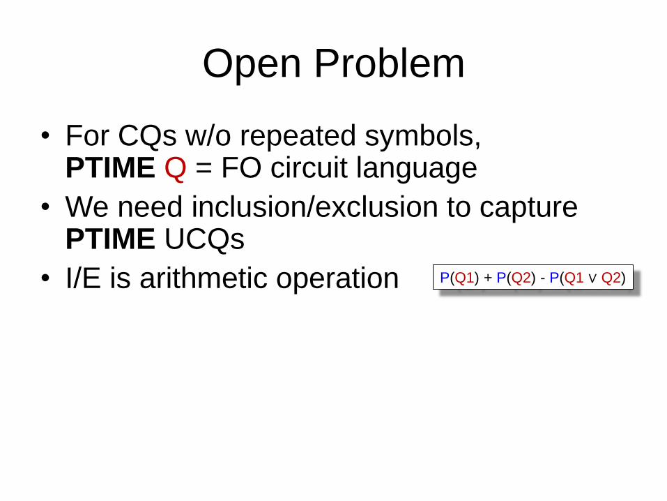
Open Problem
• For CQs w/o repeated symbols, PTIME Q = FO circuit language
• We need inclusion/exclusion to capture PTIME UCQs
• I/E is arithmetic operation
P(Q1) + P(Q2) - P(Q1 ∨ Q2)
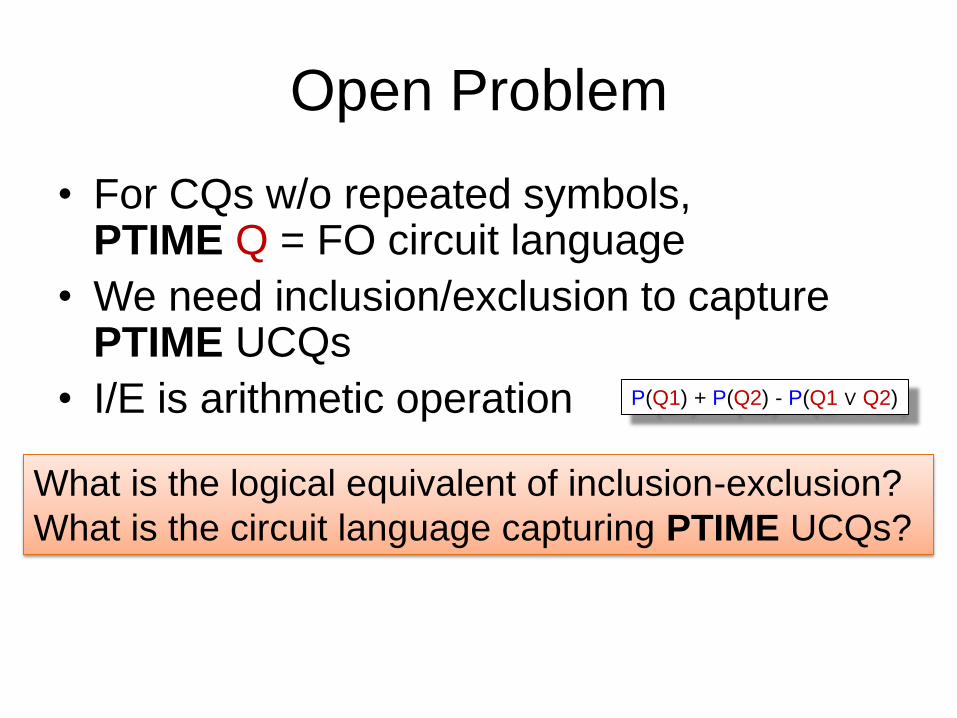
Open Problem
• For CQs w/o repeated symbols, PTIME Q = FO circuit language
• We need inclusion/exclusion to capture PTIME UCQs
• I/E is arithmetic operation
P(Q1) + P(Q2) - P(Q1 ∨ Q2)
What is the logical equivalent of inclusion-exclusion?
What is the circuit language capturing PTIME UCQs?
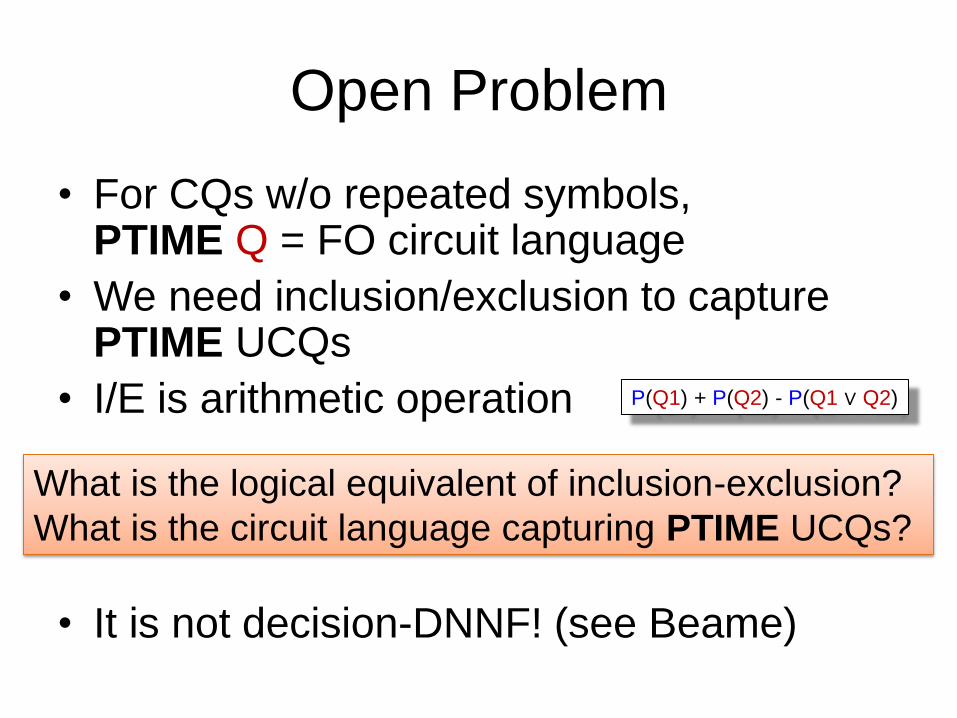
Open Problem
• For CQs w/o repeated symbols, PTIME Q = FO circuit language
• We need inclusion/exclusion to capture PTIME UCQs
• I/E is arithmetic operation
• It is not decision-DNNF! (see Beame)
P(Q1) + P(Q2) - P(Q1 ∨ Q2)
What is the logical equivalent of inclusion-exclusion?
What is the circuit language capturing PTIME UCQs?
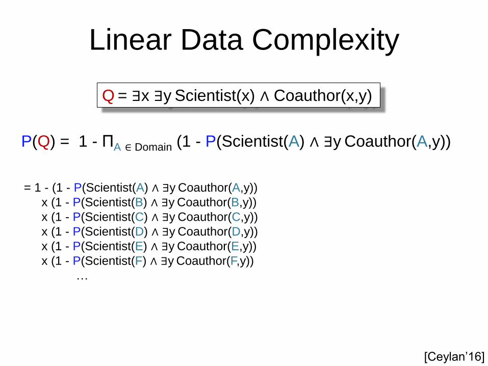
Linear Data Complexity
Q = ∃x ∃y Scientist(x) ∧ Coauthor(x,y)
P(Q) = 1 - ΠA ∈ Domain (1 - P(Scientist(A) ∧ ∃y Coauthor(A,y))
= 1 - (1 - P(Scientist(A) ∧ ∃y Coauthor(A,y))
x (1 - P(Scientist(B) ∧ ∃y Coauthor(B,y))
x (1 - P(Scientist(C) ∧ ∃y Coauthor(C,y))
x (1 - P(Scientist(D) ∧ ∃y Coauthor(D,y))
x (1 - P(Scientist(E) ∧ ∃y Coauthor(E,y))
x (1 - P(Scientist(F) ∧ ∃y Coauthor(F,y))
…
[Ceylan‟16]
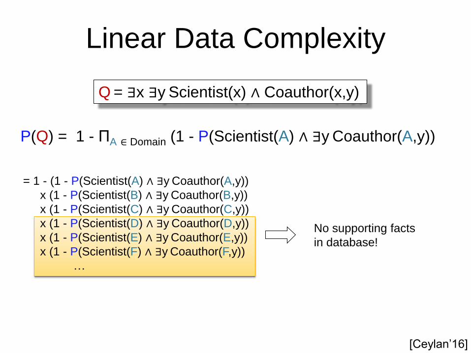
Linear Data Complexity
No supporting facts
in database!
Q = ∃x ∃y Scientist(x) ∧ Coauthor(x,y)
P(Q) = 1 - ΠA ∈ Domain (1 - P(Scientist(A) ∧ ∃y Coauthor(A,y))
= 1 - (1 - P(Scientist(A) ∧ ∃y Coauthor(A,y))
x (1 - P(Scientist(B) ∧ ∃y Coauthor(B,y))
x (1 - P(Scientist(C) ∧ ∃y Coauthor(C,y))
x (1 - P(Scientist(D) ∧ ∃y Coauthor(D,y))
x (1 - P(Scientist(E) ∧ ∃y Coauthor(E,y))
x (1 - P(Scientist(F) ∧ ∃y Coauthor(F,y))
…
[Ceylan‟16]

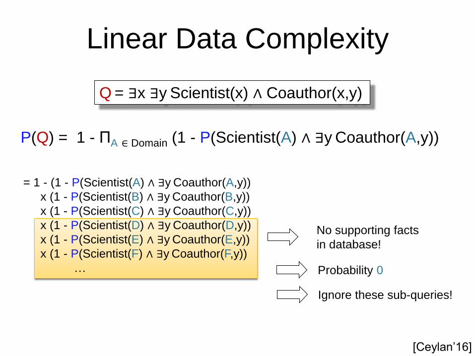
Linear Data Complexity
No supporting facts
in database!
Probability 0
Q = ∃x ∃y Scientist(x) ∧ Coauthor(x,y)
P(Q) = 1 - ΠA ∈ Domain (1 - P(Scientist(A) ∧ ∃y Coauthor(A,y))
= 1 - (1 - P(Scientist(A) ∧ ∃y Coauthor(A,y))
x (1 - P(Scientist(B) ∧ ∃y Coauthor(B,y))
x (1 - P(Scientist(C) ∧ ∃y Coauthor(C,y))
x (1 - P(Scientist(D) ∧ ∃y Coauthor(D,y))
x (1 - P(Scientist(E) ∧ ∃y Coauthor(E,y))
x (1 - P(Scientist(F) ∧ ∃y Coauthor(F,y))
…
[Ceylan‟16]
Linear Data Complexity
No supporting facts
in database!
Probability 0
Ignore these sub-queries!
Q = ∃x ∃y Scientist(x) ∧ Coauthor(x,y)
P(Q) = 1 - ΠA ∈ Domain (1 - P(Scientist(A) ∧ ∃y Coauthor(A,y))
= 1 - (1 - P(Scientist(A) ∧ ∃y Coauthor(A,y))
x (1 - P(Scientist(B) ∧ ∃y Coauthor(B,y))
x (1 - P(Scientist(C) ∧ ∃y Coauthor(C,y))
x (1 - P(Scientist(D) ∧ ∃y Coauthor(D,y))
x (1 - P(Scientist(E) ∧ ∃y Coauthor(E,y))
x (1 - P(Scientist(F) ∧ ∃y Coauthor(F,y))
…
[Ceylan‟16]
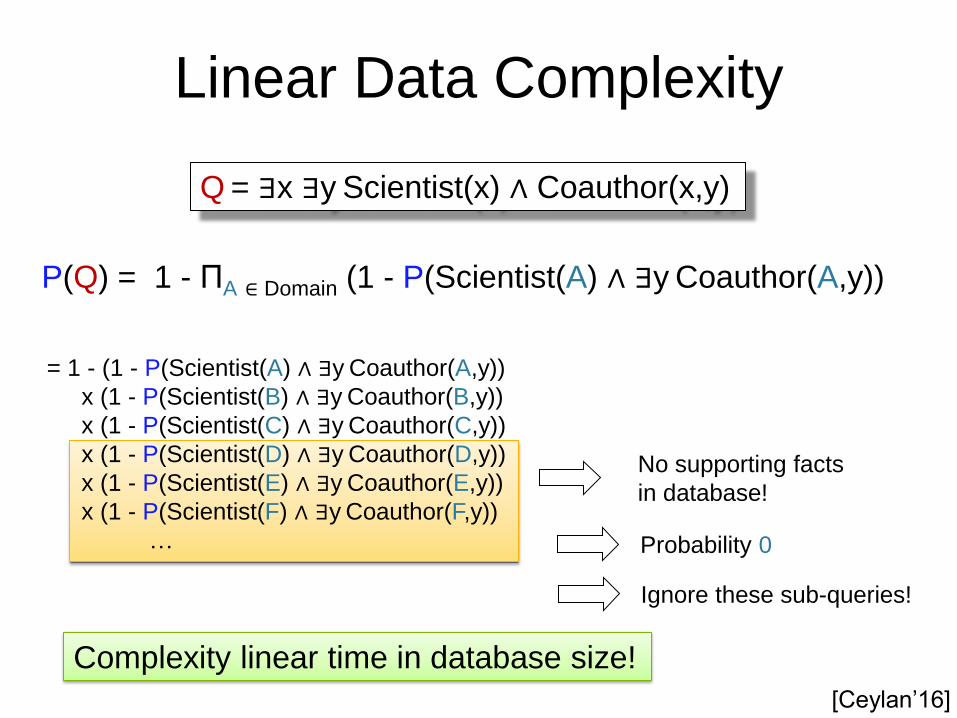
Linear Data Complexity
No supporting facts
in database!
Complexity linear time in database size!
Probability 0
Ignore these sub-queries!
Q = ∃x ∃y Scientist(x) ∧ Coauthor(x,y)
P(Q) = 1 - ΠA ∈ Domain (1 - P(Scientist(A) ∧ ∃y Coauthor(A,y))
= 1 - (1 - P(Scientist(A) ∧ ∃y Coauthor(A,y))
x (1 - P(Scientist(B) ∧ ∃y Coauthor(B,y))
x (1 - P(Scientist(C) ∧ ∃y Coauthor(C,y))
x (1 - P(Scientist(D) ∧ ∃y Coauthor(D,y))
x (1 - P(Scientist(E) ∧ ∃y Coauthor(E,y))
x (1 - P(Scientist(F) ∧ ∃y Coauthor(F,y))
…
[Ceylan‟16]

Commercial Break
• Survey book (2017)
• Survey book (2011)
• IJCAI 2016 tutorial http://web.cs.ucla.edu/~guyvdb/talks/IJCAI16-tutorial/
Overview
1. Propositional Refresher
2. Primer: A First-Order Tractable Language
3. Probabilistic Databases
4. Symmetric First-Order Model Counting
5. Lots of Pointers
...
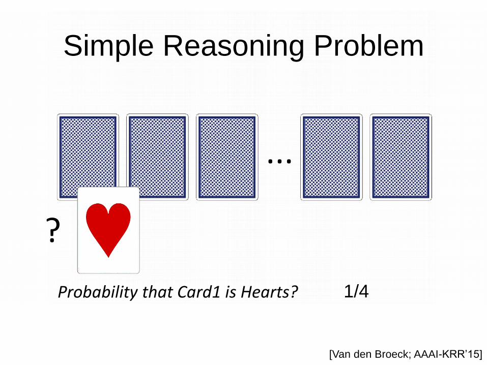
Simple Reasoning Problem
?
Probability that Card1 is Hearts? 1/4
[Van den Broeck; AAAI-KRR‟15]
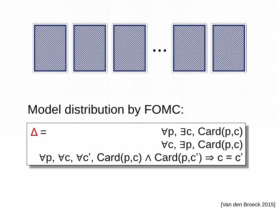
Model distribution by FOMC:
...
∀p, ∃c, Card(p,c)
∀c, ∃p, Card(p,c)
∀p, ∀c, ∀c‟, Card(p,c) ∧ Card(p,c‟) ⇒ c = c‟
Δ =
[Van den Broeck 2015]
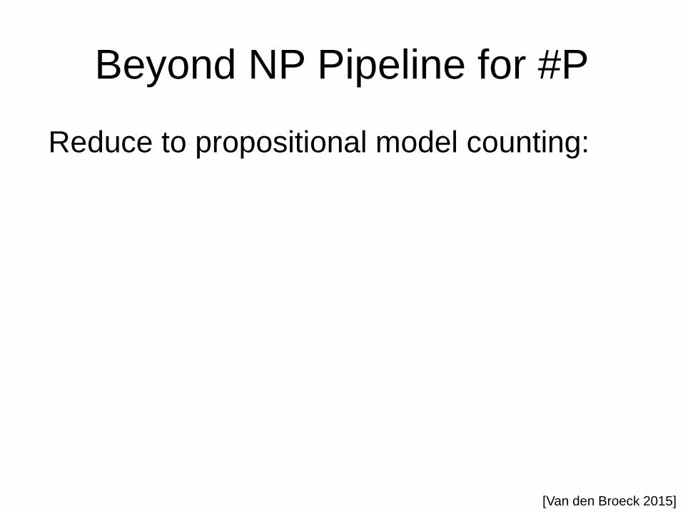
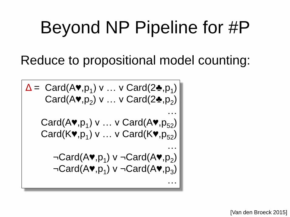
Beyond NP Pipeline for #P
Reduce to propositional model counting:
[Van den Broeck 2015]
Beyond NP Pipeline for #P
Reduce to propositional model counting:
Card(A♥,p1) v … v Card(2♣,p1)
Card(A♥,p2) v … v Card(2♣,p2)
…
Card(A♥,p1) v … v Card(A♥,p52)
Card(K♥,p1) v … v Card(K♥,p52)
…
¬Card(A♥,p1) v ¬Card(A♥,p2)
¬Card(A♥,p1) v ¬Card(A♥,p3)
…
Δ =
[Van den Broeck 2015]
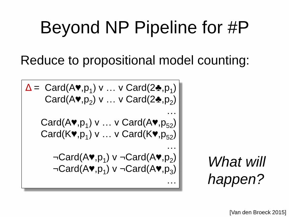
Beyond NP Pipeline for #P
Reduce to propositional model counting:
Card(A♥,p1) v … v Card(2♣,p1)
Card(A♥,p2) v … v Card(2♣,p2)
…
Card(A♥,p1) v … v Card(A♥,p52)
Card(K♥,p1) v … v Card(K♥,p52)
…
¬Card(A♥,p1) v ¬Card(A♥,p2)
¬Card(A♥,p1) v ¬Card(A♥,p3)
…
Δ =
What will
happen?
[Van den Broeck 2015]
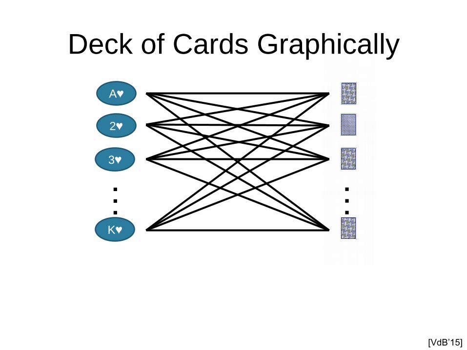
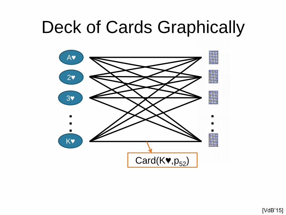
Deck of Cards Graphically
K♥
A♥
2♥
3♥
…
…
[VdB‟15]

Deck of Cards Graphically
K♥
A♥
2♥
3♥
…
…
Card(K♥,p52)
[VdB‟15]
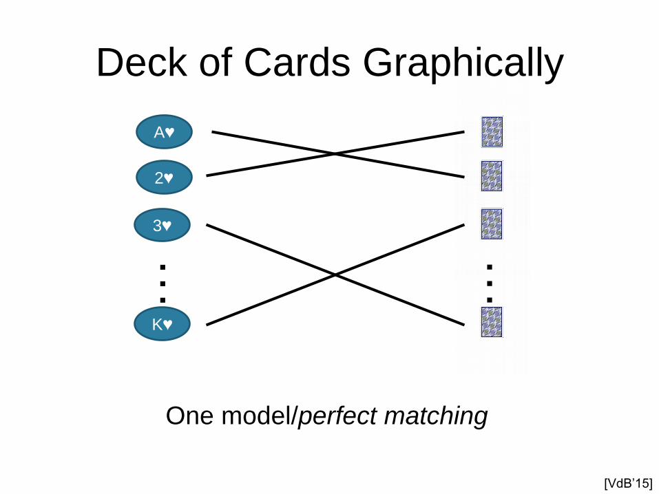
Deck of Cards Graphically
K♥
A♥
2♥
3♥
…
…
One model/perfect matching
[VdB‟15]

Deck of Cards Graphically
K♥
A♥
2♥
3♥
…
…
[VdB‟15]
Deck of Cards Graphically
K♥
A♥
2♥
3♥
…
…
Card(K♥,p52)
[VdB‟15]
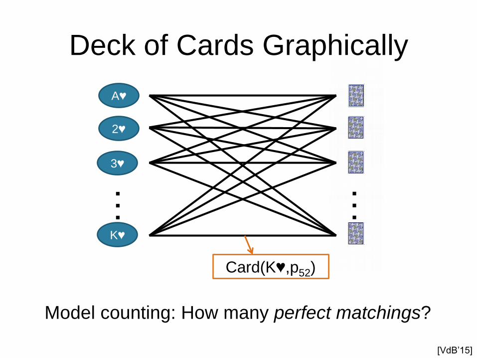
Deck of Cards Graphically
K♥
A♥
2♥
3♥
…
…
Card(K♥,p52)
Model counting: How many perfect matchings?
[VdB‟15]
Deck of Cards Graphically
K♥
A♥
2♥
3♥
…
…
[VdB‟15]
What if I set
w(Card(K♥,p52)) = 0?
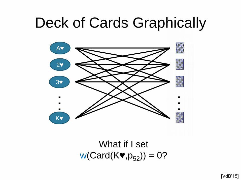
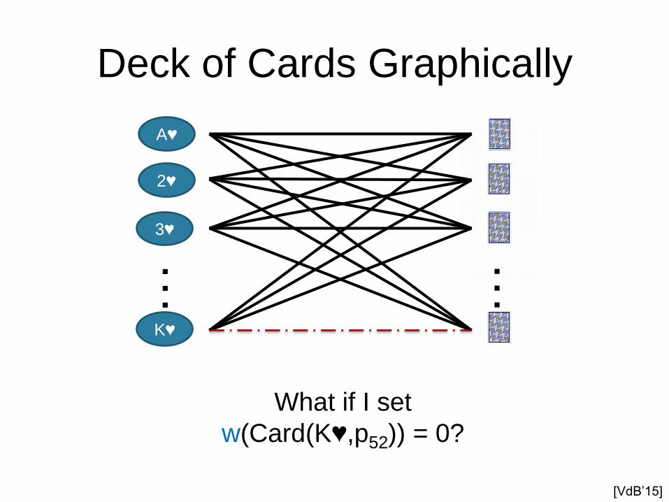
Deck of Cards Graphically
K♥
A♥
2♥
3♥
…
…
What if I set
w(Card(K♥,p52)) = 0?
[VdB‟15]
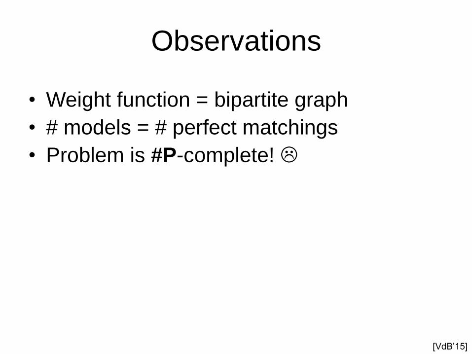
Observations
• Weight function = bipartite graph
• # models = # perfect matchings
• Problem is #P-complete!
[VdB‟15]

Observations
• Weight function = bipartite graph
• # models = # perfect matchings
• Problem is #P-complete!
[VdB‟15]
No propositional WMC solver can
handle cards problem efficiently!
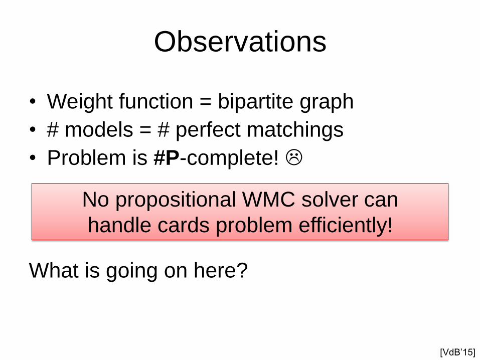
Observations
• Weight function = bipartite graph
• # models = # perfect matchings
• Problem is #P-complete!
What is going on here?
[VdB‟15]
No propositional WMC solver can
handle cards problem efficiently!
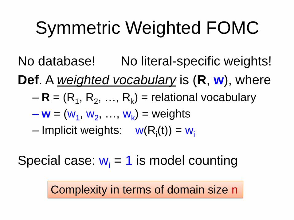
Symmetric Weighted FOMC
No database! No literal-specific weights!
Def. A weighted vocabulary is (R, w), where
– R = (R1, R2, …, Rk) = relational vocabulary
– w = (w1, w2, …, wk) = weights
– Implicit weights: w(Ri(t)) = wi
Special case: wi = 1 is model counting
Complexity in terms of domain size n
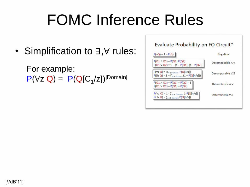
FOMC Inference Rules
• Simplification to ∃,∀ rules:
For example:
P(∀z Q) = P(Q[C1/z])|Domain|
[VdB‟11]
FOMC Inference Rules
• Simplification to ∃,∀ rules:
For example:
P(∀z Q) = P(Q[C1/z])|Domain|
The workhorse
of FOMC
• A powerful new inference rule: atom counting
Only possible with symmetric weights
Intuition: Remove unary relations
[VdB‟11]
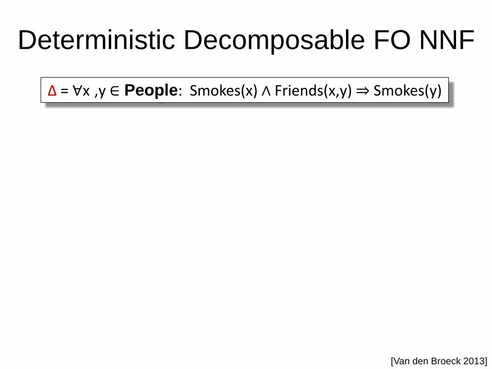
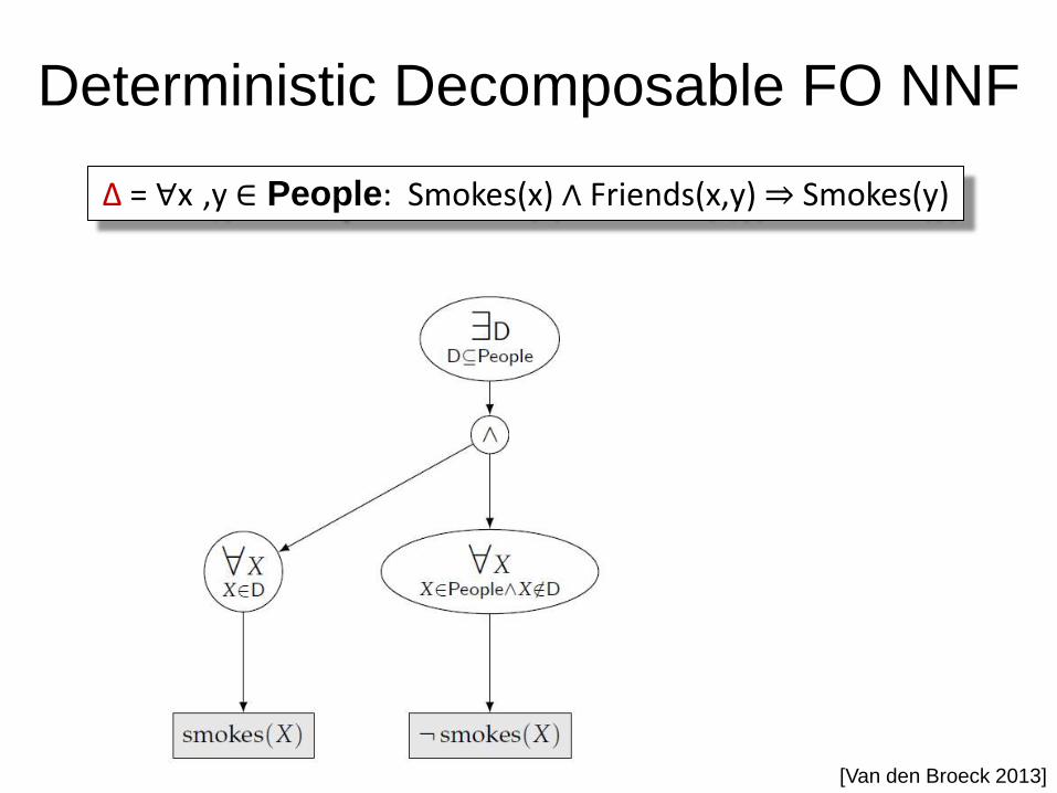
Deterministic Decomposable FO NNF
[Van den Broeck 2013]
Δ = ∀x ,y ∈ People: Smokes(x) ∧ Friends(x,y) ⇒ Smokes(y)
Δ = ∀x ,y ∈ People: Smokes(x) ∧ Friends(x,y) ⇒ Smokes(y)
[Van den Broeck 2013]
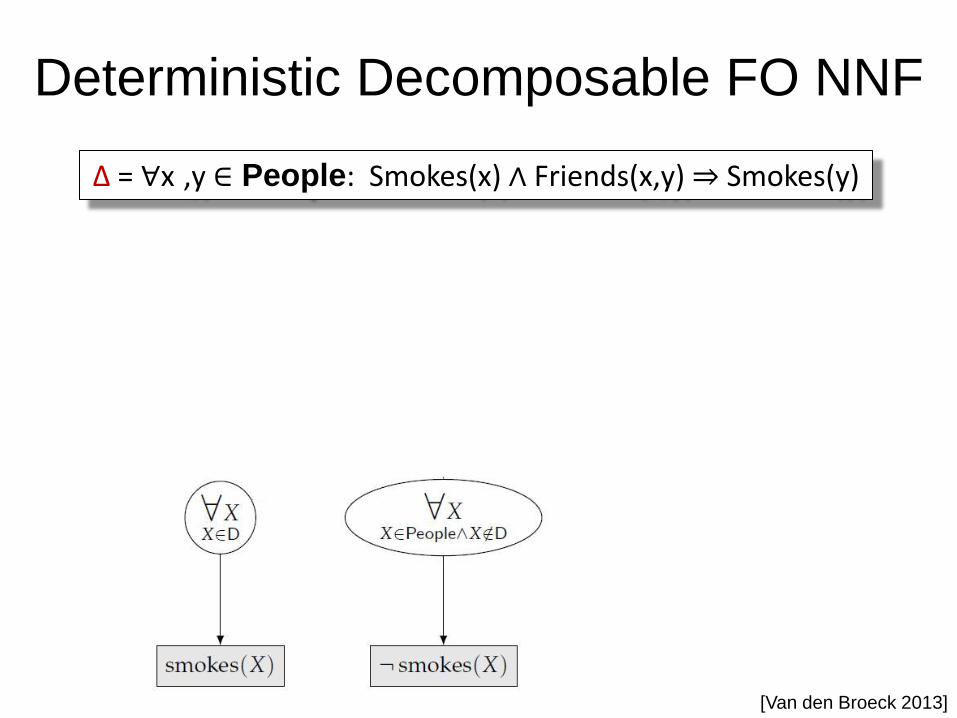
Deterministic Decomposable FO NNF
[Van den Broeck 2013]
Δ = ∀x ,y ∈ People: Smokes(x) ∧ Friends(x,y) ⇒ Smokes(y)
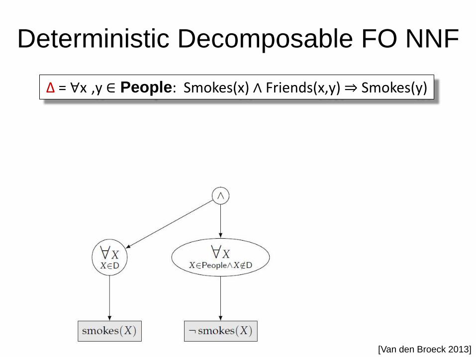
Deterministic Decomposable FO NNF
[Van den Broeck 2013]
Δ = ∀x ,y ∈ People: Smokes(x) ∧ Friends(x,y) ⇒ Smokes(y)
Deterministic Decomposable FO NNF
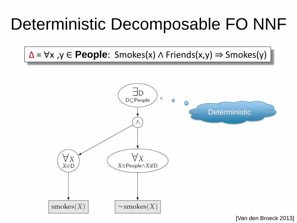
Deterministic
[Van den Broeck 2013]
Δ = ∀x ,y ∈ People: Smokes(x) ∧ Friends(x,y) ⇒ Smokes(y)
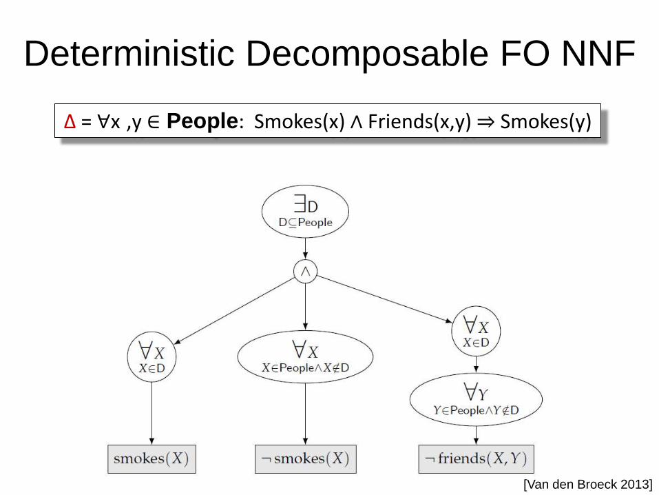
Deterministic Decomposable FO NNF
[Van den Broeck 2013]
Δ = ∀x ,y ∈ People: Smokes(x) ∧ Friends(x,y) ⇒ Smokes(y)
Deterministic Decomposable FO NNF
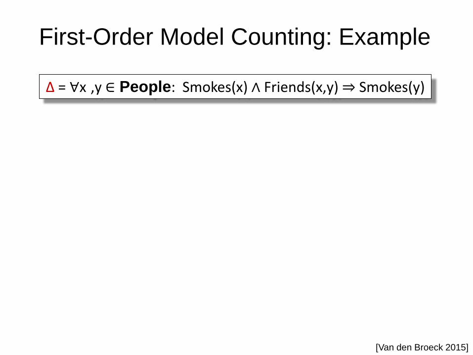
First-Order Model Counting: Example
[Van den Broeck 2015]
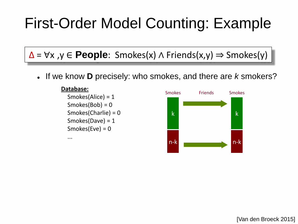
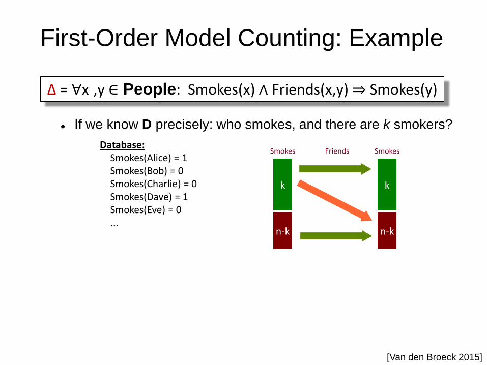
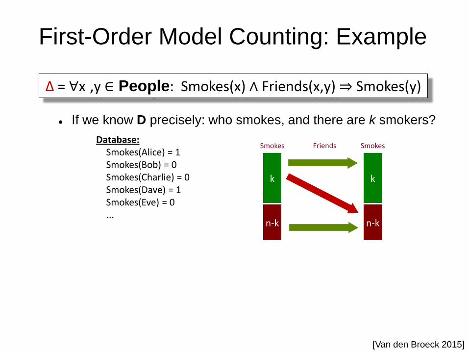
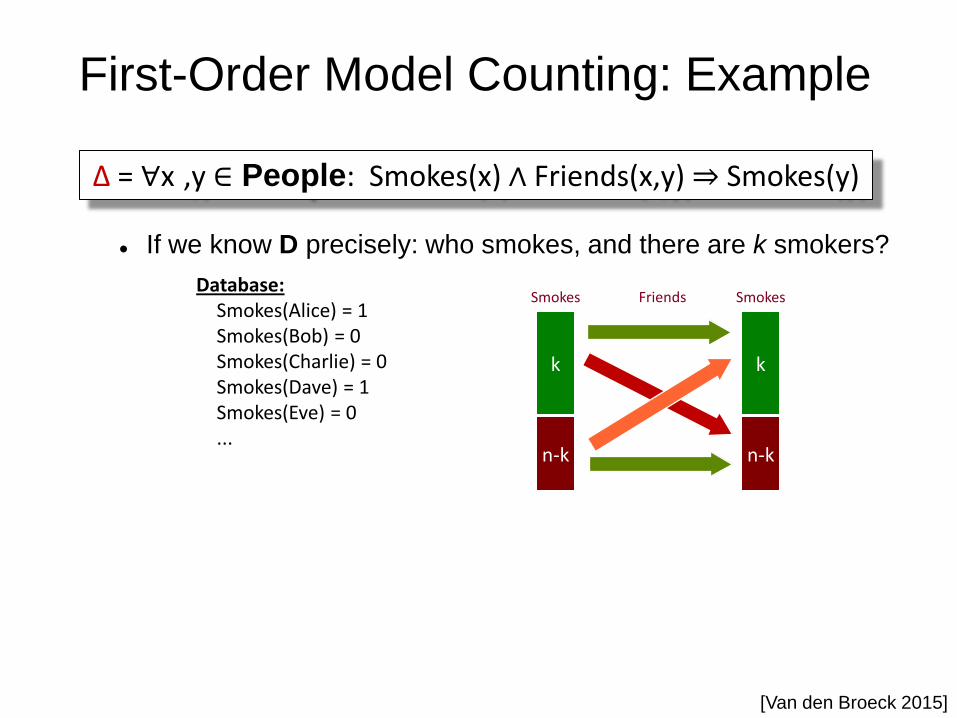
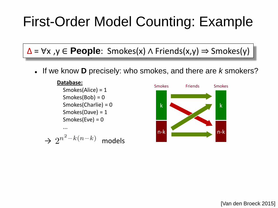
Δ = ∀x ,y ∈ People: Smokes(x) ∧ Friends(x,y) ⇒ Smokes(y)
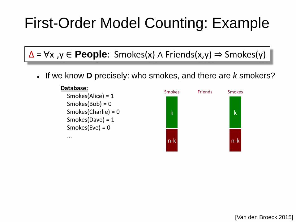
First-Order Model Counting: Example
If we know D precisely: who smokes, and there are k smokers?
k
n-k
k
n-k
Database: Smokes(Alice) = 1 Smokes(Bob) = 0 Smokes(Charlie) = 0 Smokes(Dave) = 1 Smokes(Eve) = 0 ...
Smokes Smokes Friends
[Van den Broeck 2015]
Δ = ∀x ,y ∈ People: Smokes(x) ∧ Friends(x,y) ⇒ Smokes(y)
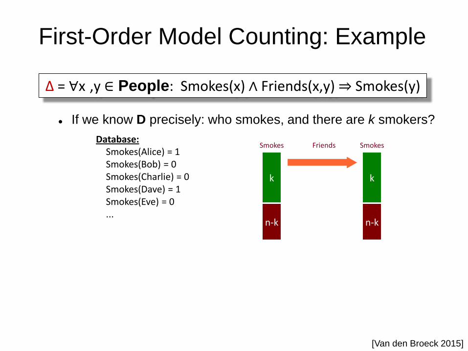
First-Order Model Counting: Example
If we know D precisely: who smokes, and there are k smokers?
k
n-k
k
n-k
Database: Smokes(Alice) = 1 Smokes(Bob) = 0 Smokes(Charlie) = 0 Smokes(Dave) = 1 Smokes(Eve) = 0 ...
Smokes Smokes Friends
[Van den Broeck 2015]
Δ = ∀x ,y ∈ People: Smokes(x) ∧ Friends(x,y) ⇒ Smokes(y)
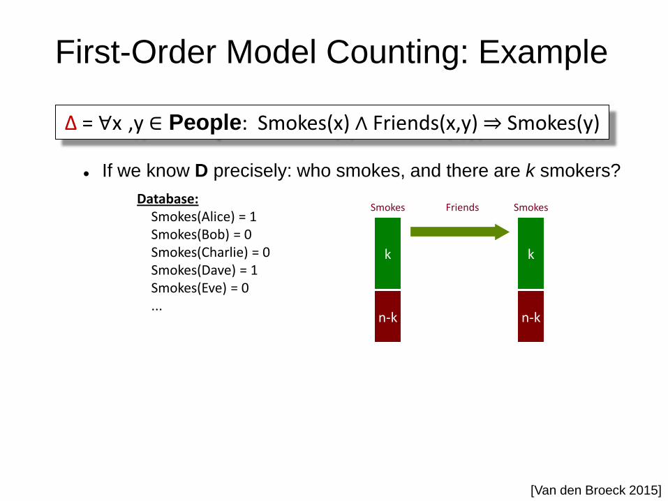
First-Order Model Counting: Example
If we know D precisely: who smokes, and there are k smokers?
k
n-k
k
n-k
Database: Smokes(Alice) = 1 Smokes(Bob) = 0 Smokes(Charlie) = 0 Smokes(Dave) = 1 Smokes(Eve) = 0 ...
Smokes Smokes Friends
[Van den Broeck 2015]
Δ = ∀x ,y ∈ People: Smokes(x) ∧ Friends(x,y) ⇒ Smokes(y)
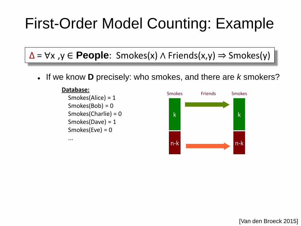
First-Order Model Counting: Example
If we know D precisely: who smokes, and there are k smokers?
k
n-k
k
n-k
Database: Smokes(Alice) = 1 Smokes(Bob) = 0 Smokes(Charlie) = 0 Smokes(Dave) = 1 Smokes(Eve) = 0 ...
Smokes Smokes Friends
[Van den Broeck 2015]
Δ = ∀x ,y ∈ People: Smokes(x) ∧ Friends(x,y) ⇒ Smokes(y)
First-Order Model Counting: Example
If we know D precisely: who smokes, and there are k smokers?
k
n-k
k
n-k
→ models
Database: Smokes(Alice) = 1 Smokes(Bob) = 0 Smokes(Charlie) = 0 Smokes(Dave) = 1 Smokes(Eve) = 0 ...
Smokes Smokes Friends
[Van den Broeck 2015]
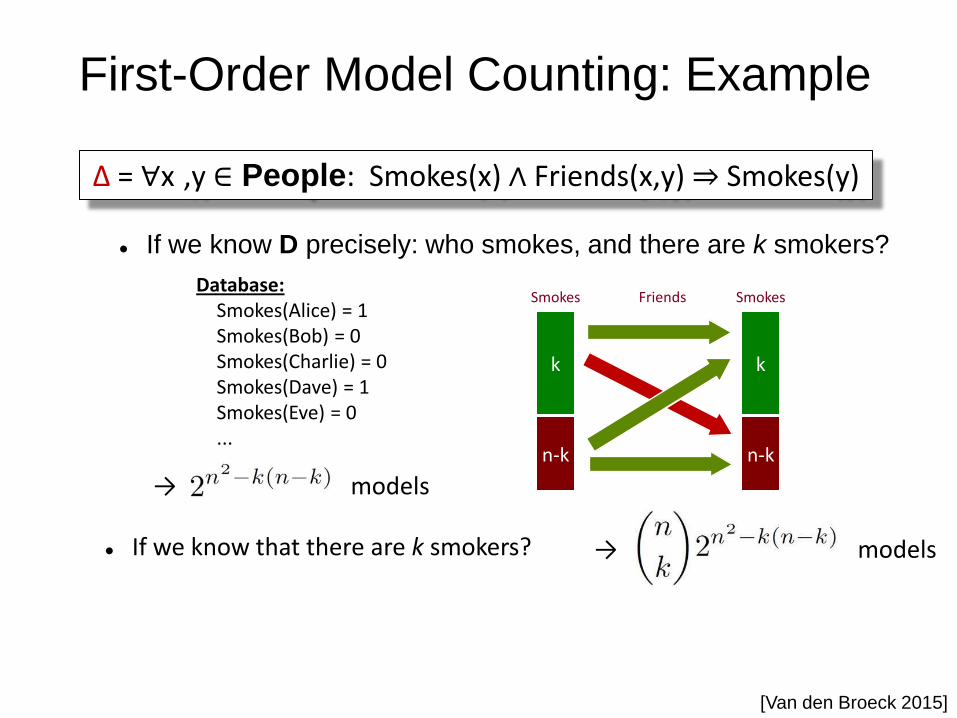
Δ = ∀x ,y ∈ People: Smokes(x) ∧ Friends(x,y) ⇒ Smokes(y)

First-Order Model Counting: Example
If we know D precisely: who smokes, and there are k smokers?
k
n-k
k
n-k
If we know that there are k smokers?
→ models
Database: Smokes(Alice) = 1 Smokes(Bob) = 0 Smokes(Charlie) = 0 Smokes(Dave) = 1 Smokes(Eve) = 0 ...
Smokes Smokes Friends
[Van den Broeck 2015]
Δ = ∀x ,y ∈ People: Smokes(x) ∧ Friends(x,y) ⇒ Smokes(y)
First-Order Model Counting: Example
If we know D precisely: who smokes, and there are k smokers?
k
n-k
k
n-k
If we know that there are k smokers?
→ models
Database: Smokes(Alice) = 1 Smokes(Bob) = 0 Smokes(Charlie) = 0 Smokes(Dave) = 1 Smokes(Eve) = 0 ...
→ models
Smokes Smokes Friends
[Van den Broeck 2015]
Δ = ∀x ,y ∈ People: Smokes(x) ∧ Friends(x,y) ⇒ Smokes(y)

First-Order Model Counting: Example
If we know D precisely: who smokes, and there are k smokers?
k
n-k
k
n-k
If we know that there are k smokers?
In total…
→ models
Database: Smokes(Alice) = 1 Smokes(Bob) = 0 Smokes(Charlie) = 0 Smokes(Dave) = 1 Smokes(Eve) = 0 ...
→ models
Smokes Smokes Friends
[Van den Broeck 2015]
Δ = ∀x ,y ∈ People: Smokes(x) ∧ Friends(x,y) ⇒ Smokes(y)
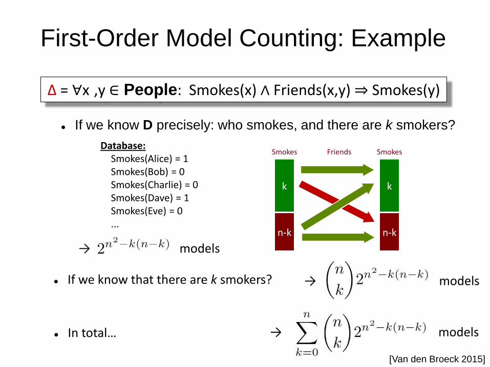
First-Order Model Counting: Example
If we know D precisely: who smokes, and there are k smokers?
k
n-k
k
n-k
If we know that there are k smokers?
In total…
→ models
Database: Smokes(Alice) = 1 Smokes(Bob) = 0 Smokes(Charlie) = 0 Smokes(Dave) = 1 Smokes(Eve) = 0 ...
→ models
→ models
Smokes Smokes Friends
[Van den Broeck 2015]
Δ = ∀x ,y ∈ People: Smokes(x) ∧ Friends(x,y) ⇒ Smokes(y)
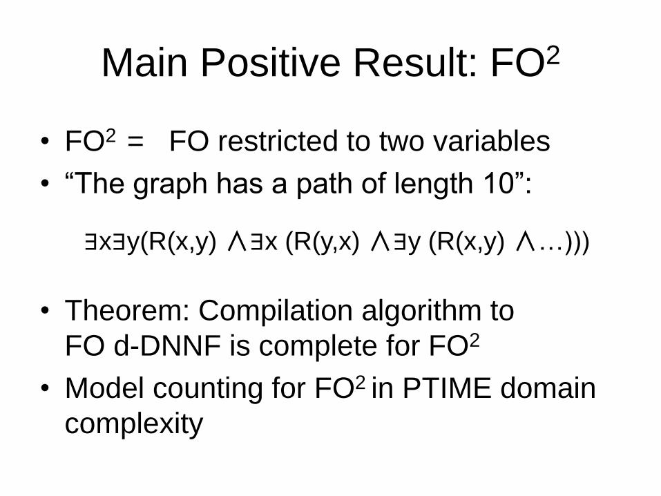
Main Positive Result: FO2
• FO2 = FO restricted to two variables
• “The graph has a path of length 10”:
• Theorem: Compilation algorithm to
FO d-DNNF is complete for FO2
• Model counting for FO2 in PTIME domain
complexity
∃x∃y(R(x,y) ∧∃x (R(y,x) ∧∃y (R(x,y) ∧…)))
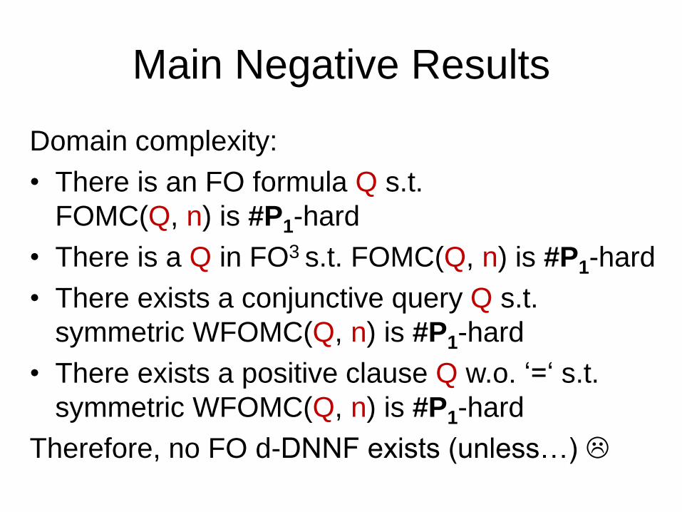
Main Negative Results
Domain complexity:
• There is an FO formula Q s.t.
FOMC(Q, n) is #P1-hard
• There is a Q in FO3 s.t. FOMC(Q, n) is #P1-hard
• There exists a conjunctive query Q s.t.
symmetric WFOMC(Q, n) is #P1-hard
• There exists a positive clause Q w.o. „=„ s.t.
symmetric WFOMC(Q, n) is #P1-hard
Therefore, no FO d-DNNF exists (unless…)
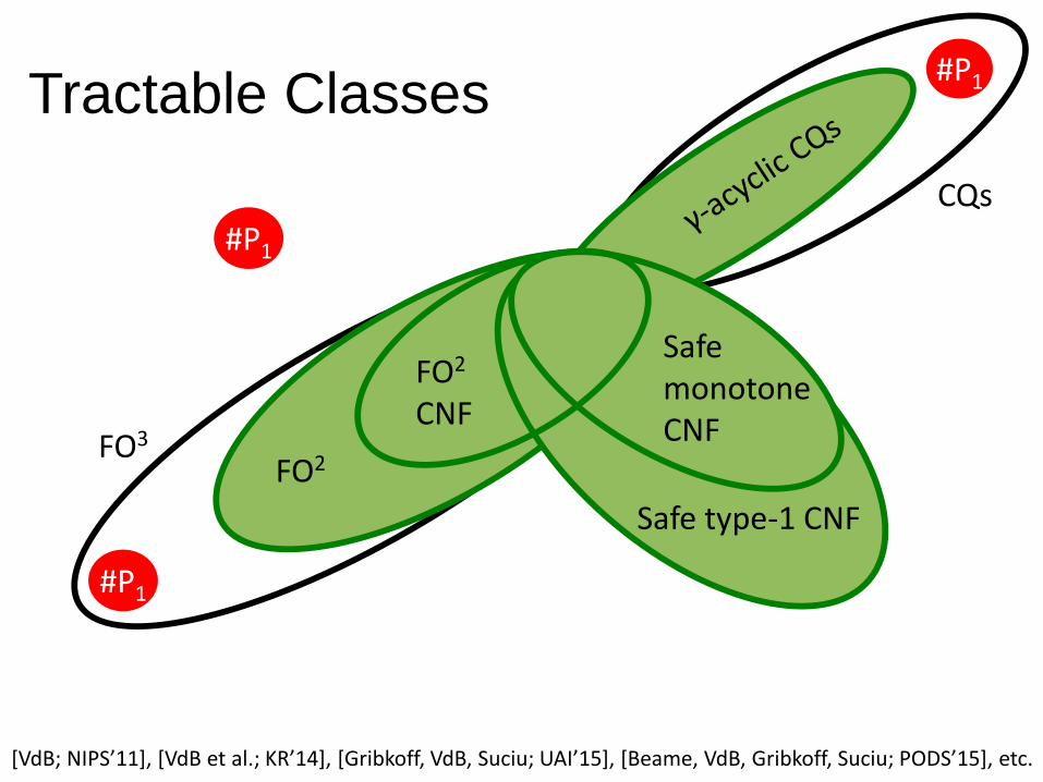
Tractable Classes
FO2
CNF
FO2
Safe monotone CNF Safe type-1 CNF
#P1
FO3
#P1
CQs
[VdB; NIPS’11+, [VdB et al.; KR’14], [Gribkoff, VdB, Suciu; UAI’15+, [Beame, VdB, Gribkoff, Suciu; PODS’15+, etc.
#P1
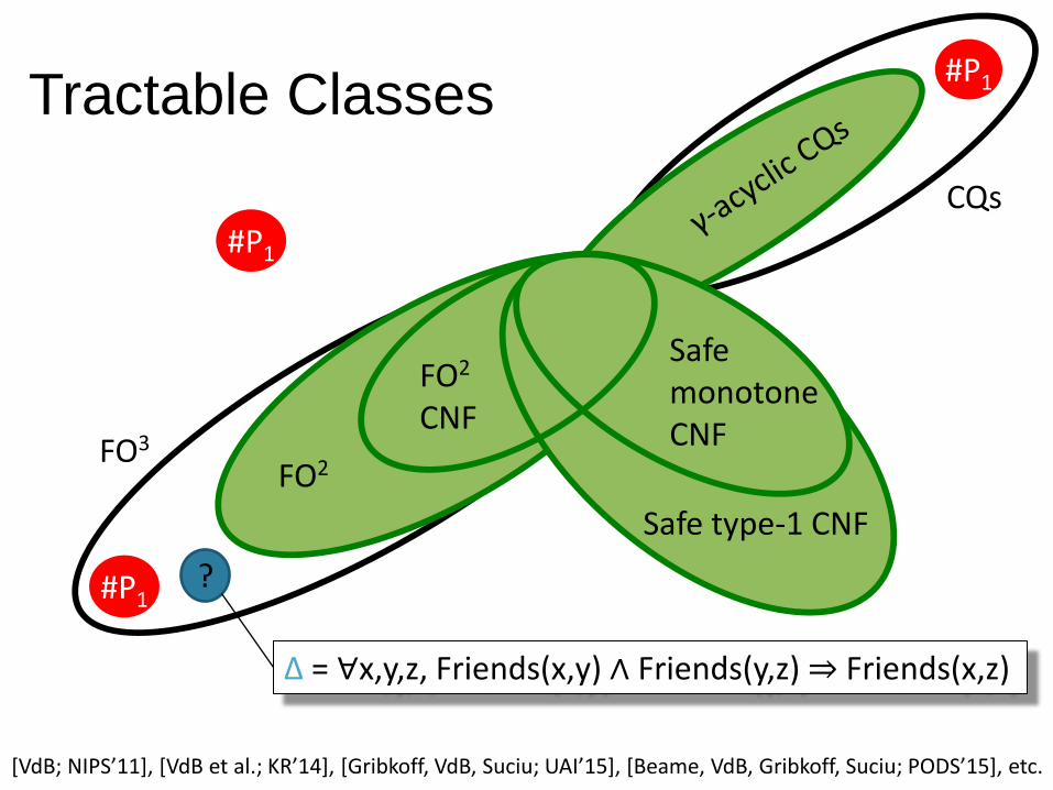
Tractable Classes
FO2
CNF
FO2
Safe monotone CNF Safe type-1 CNF
? #P1
FO3
#P1
CQs
Δ = ∀x,y,z, Friends(x,y) ∧ Friends(y,z) ⇒ Friends(x,z)
[VdB; NIPS’11+, [VdB et al.; KR’14], [Gribkoff, VdB, Suciu; UAI’15+, [Beame, VdB, Gribkoff, Suciu; PODS’15+, etc.
#P1
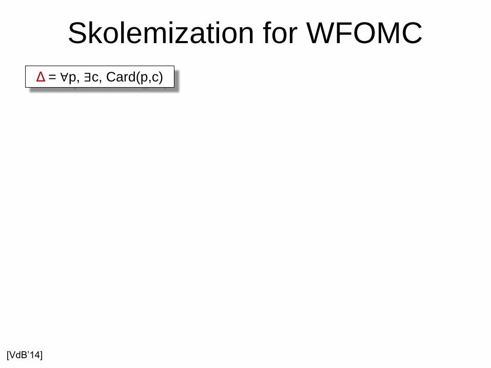
Skolemization for WFOMC
Δ = ∀p, ∃c, Card(p,c)
[VdB‟14]
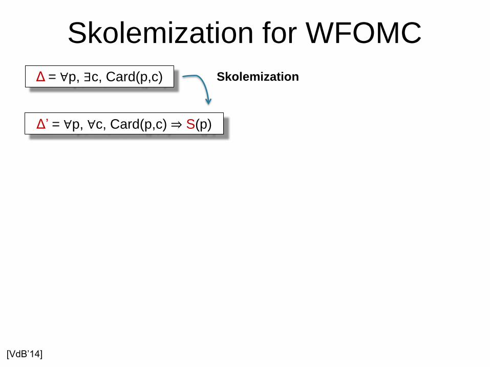
Skolemization
Skolemization for WFOMC
Δ = ∀p, ∃c, Card(p,c)
Δ‟ = ∀p, ∀c, Card(p,c) ⇒ S(p)
[VdB‟14]

w(S) = 1 and w(¬S) = -1
Skolemization
Skolem predicate
Skolemization for WFOMC
Δ = ∀p, ∃c, Card(p,c)
Δ‟ = ∀p, ∀c, Card(p,c) ⇒ S(p)
[VdB‟14]
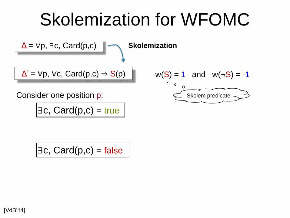
∃c, Card(p,c) = true
Consider one position p:
w(S) = 1 and w(¬S) = -1
∃c, Card(p,c) = false
Skolemization
Skolem predicate
Skolemization for WFOMC
Δ = ∀p, ∃c, Card(p,c)
Δ‟ = ∀p, ∀c, Card(p,c) ⇒ S(p)
[VdB‟14]
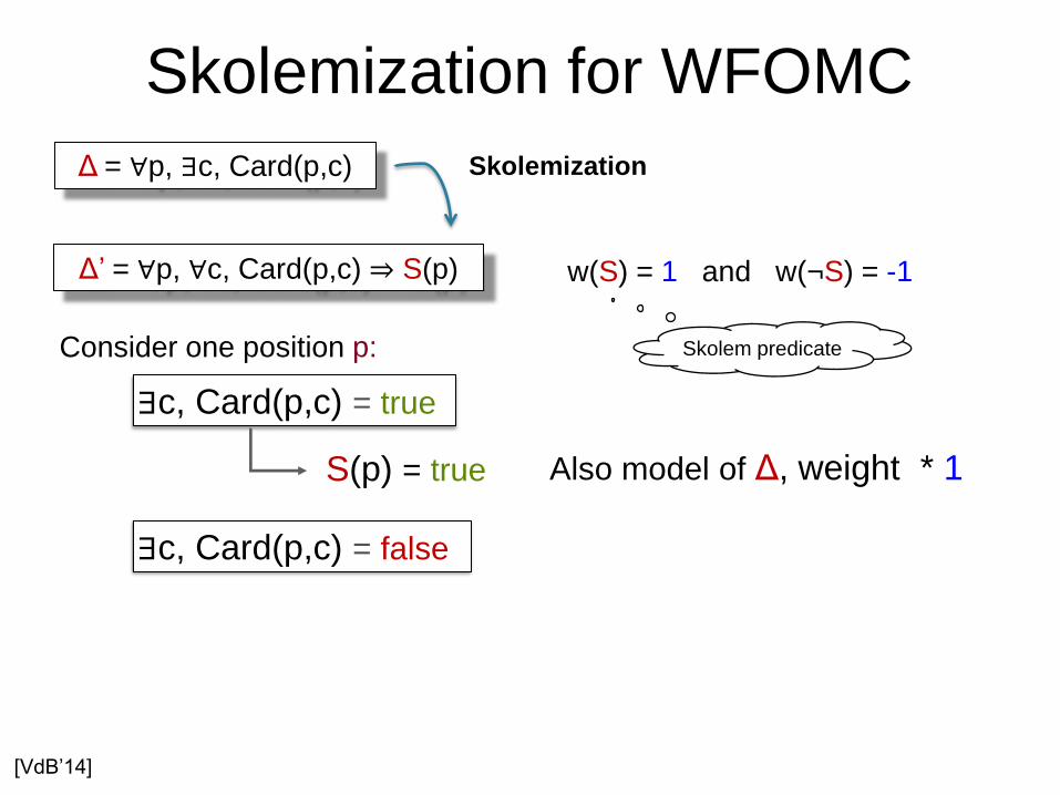
∃c, Card(p,c) = true
S(p) = true Also model of Δ, weight * 1
Consider one position p:
w(S) = 1 and w(¬S) = -1
∃c, Card(p,c) = false
Skolemization
Skolem predicate
Skolemization for WFOMC
Δ = ∀p, ∃c, Card(p,c)
Δ‟ = ∀p, ∀c, Card(p,c) ⇒ S(p)
[VdB‟14]
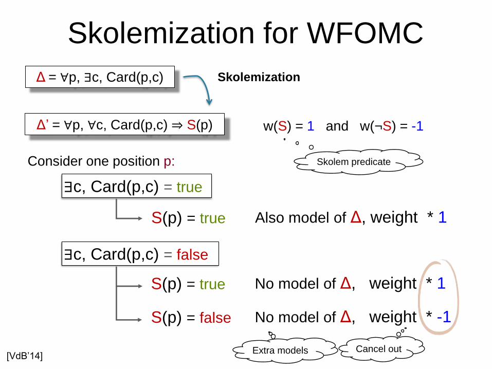
∃c, Card(p,c) = true
S(p) = true Also model of Δ, weight * 1
Consider one position p:
w(S) = 1 and w(¬S) = -1
∃c, Card(p,c) = false
S(p) = true No model of Δ, weight * 1
S(p) = false No model of Δ, weight * -1
Extra models Cancel out
Skolemization
Skolem predicate
Skolemization for WFOMC
Δ = ∀p, ∃c, Card(p,c)
Δ‟ = ∀p, ∀c, Card(p,c) ⇒ S(p)
[VdB‟14]
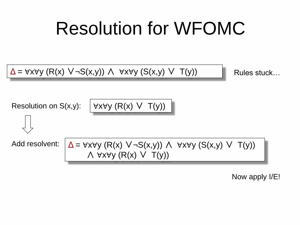
Resolution for WFOMC
Δ = ∀x∀y (R(x) ∨¬S(x,y)) ∧ ∀x∀y (S(x,y) ∨ T(y)) Rules stuck…
Add resolvent: Δ = ∀x∀y (R(x) ∨¬S(x,y)) ∧ ∀x∀y (S(x,y) ∨ T(y))
∧ ∀x∀y (R(x) ∨ T(y))
Now apply I/E!
Resolution on S(x,y): ∀x∀y (R(x) ∨ T(y))
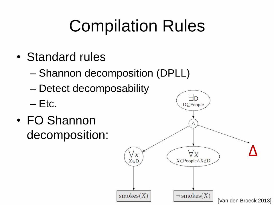
Compilation Rules
• Standard rules
– Shannon decomposition (DPLL)
– Detect decomposability
– Etc.
• FO Shannon
decomposition:
Δ
[Van den Broeck 2013]
...
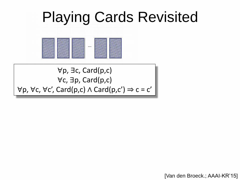
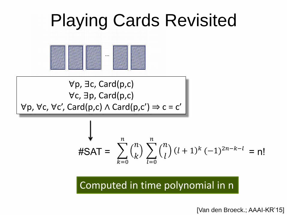
Playing Cards Revisited
∀p, ∃c, Card(p,c) ∀c, ∃p, Card(p,c)
∀p, ∀c, ∀c’, Card(p,c) ∧ Card(p,c’) ⇒ c = c’
[Van den Broeck.; AAAI-KR‟15]
...
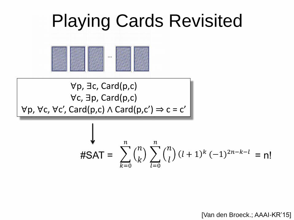
Playing Cards Revisited
∀p, ∃c, Card(p,c) ∀c, ∃p, Card(p,c)
∀p, ∀c, ∀c’, Card(p,c) ∧ Card(p,c’) ⇒ c = c’
[Van den Broeck.; AAAI-KR‟15]
...
Playing Cards Revisited
∀p, ∃c, Card(p,c) ∀c, ∃p, Card(p,c)
∀p, ∀c, ∀c’, Card(p,c) ∧ Card(p,c’) ⇒ c = c’
Computed in time polynomial in n
[Van den Broeck.; AAAI-KR‟15]
Overview
1. Propositional Refresher
2. Primer: A First-Order Tractable Language
3. Probabilistic Databases
4. Symmetric First-Order Model Counting
5. Lots of Pointers
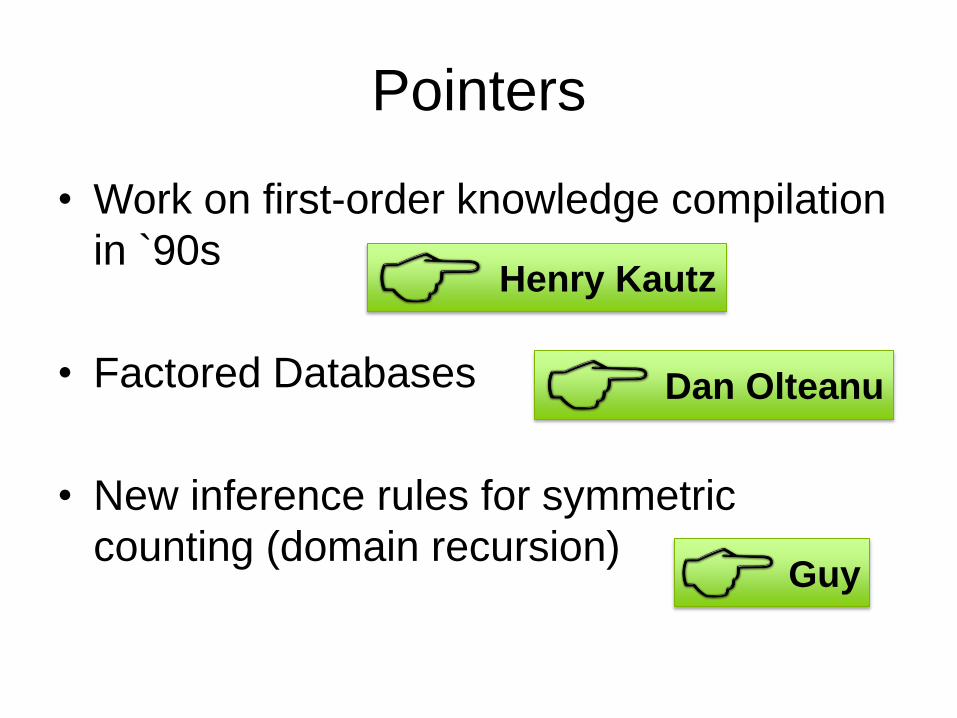
Pointers
• Work on first-order knowledge compilation
in `90s
• Factored Databases
• New inference rules for symmetric
counting (domain recursion)
Henry Kautz
Dan Olteanu
Guy
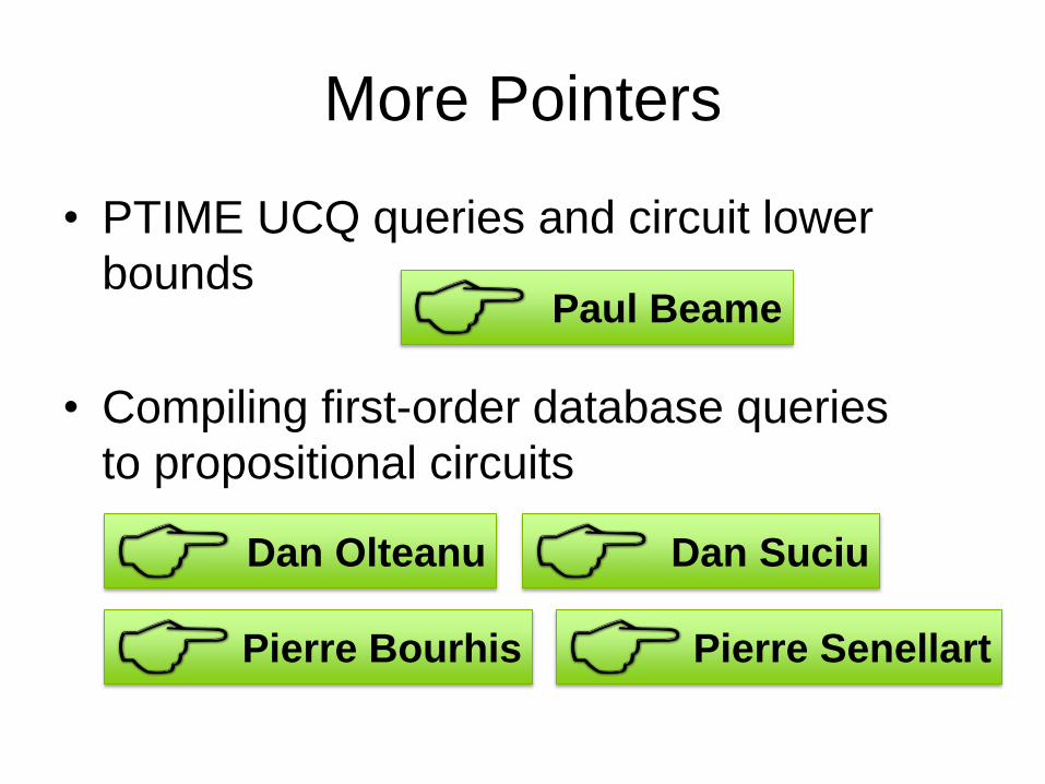
More Pointers
• PTIME UCQ queries and circuit lower
bounds
• Compiling first-order database queries
to propositional circuits
Paul Beame
Dan Olteanu Dan Suciu
Pierre Bourhis Pierre Senellart
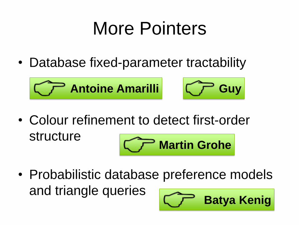
More Pointers
• Database fixed-parameter tractability
• Colour refinement to detect first-order
structure
• Probabilistic database preference models
and triangle queries
Antoine Amarilli Guy
Martin Grohe
Batya Kenig
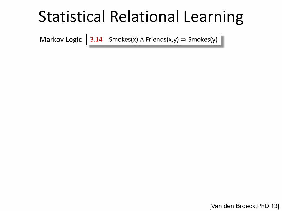
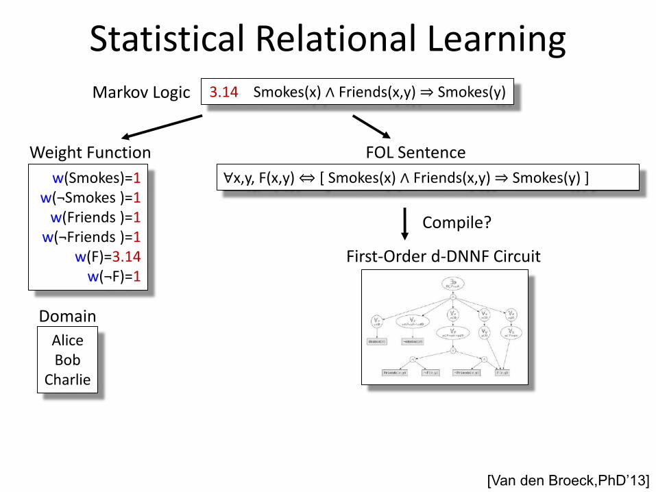
Statistical Relational Learning 3.14 Smokes(x) ∧ Friends(x,y) ⇒ Smokes(y) Markov Logic
[Van den Broeck,PhD‟13]
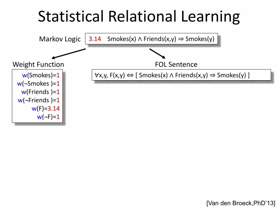
Statistical Relational Learning 3.14 Smokes(x) ∧ Friends(x,y) ⇒ Smokes(y)
∀x,y, F(x,y) ⇔ [ Smokes(x) ∧ Friends(x,y) ⇒ Smokes(y) ]
Weight Function
w(Smokes)=1 w(¬Smokes )=1 w(Friends )=1 w(¬Friends )=1
w(F)=3.14 w(¬F)=1
FOL Sentence
Markov Logic
[Van den Broeck,PhD‟13]
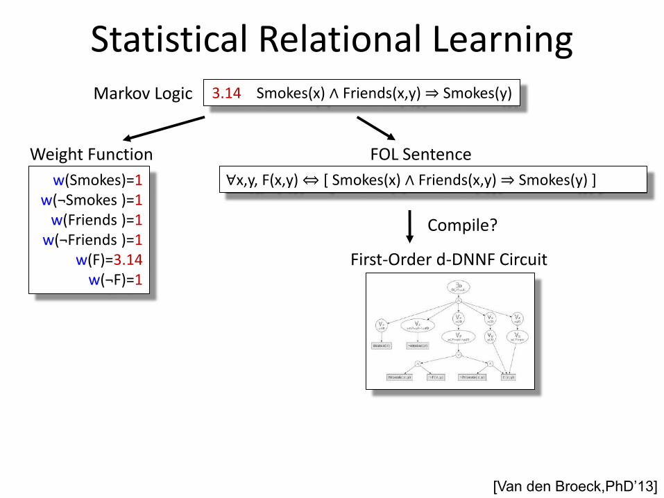
Statistical Relational Learning 3.14 Smokes(x) ∧ Friends(x,y) ⇒ Smokes(y)
∀x,y, F(x,y) ⇔ [ Smokes(x) ∧ Friends(x,y) ⇒ Smokes(y) ]
Weight Function
w(Smokes)=1 w(¬Smokes )=1 w(Friends )=1 w(¬Friends )=1
w(F)=3.14 w(¬F)=1
FOL Sentence
First-Order d-DNNF Circuit
Markov Logic
[Van den Broeck,PhD‟13]
Compile? Compile?
Statistical Relational Learning 3.14 Smokes(x) ∧ Friends(x,y) ⇒ Smokes(y)
∀x,y, F(x,y) ⇔ [ Smokes(x) ∧ Friends(x,y) ⇒ Smokes(y) ]
Weight Function
w(Smokes)=1 w(¬Smokes )=1 w(Friends )=1 w(¬Friends )=1
w(F)=3.14 w(¬F)=1
FOL Sentence
First-Order d-DNNF Circuit
Domain
Alice Bob
Charlie
Markov Logic
[Van den Broeck,PhD‟13]
Compile? Compile?

Statistical Relational Learning 3.14 Smokes(x) ∧ Friends(x,y) ⇒ Smokes(y)
∀x,y, F(x,y) ⇔ [ Smokes(x) ∧ Friends(x,y) ⇒ Smokes(y) ]
Weight Function
w(Smokes)=1 w(¬Smokes )=1 w(Friends )=1 w(¬Friends )=1
w(F)=3.14 w(¬F)=1
FOL Sentence
First-Order d-DNNF Circuit
Domain
Alice Bob
Charlie Z = WFOMC = 1479.85
Markov Logic
[Van den Broeck,PhD‟13]
Compile? Compile?
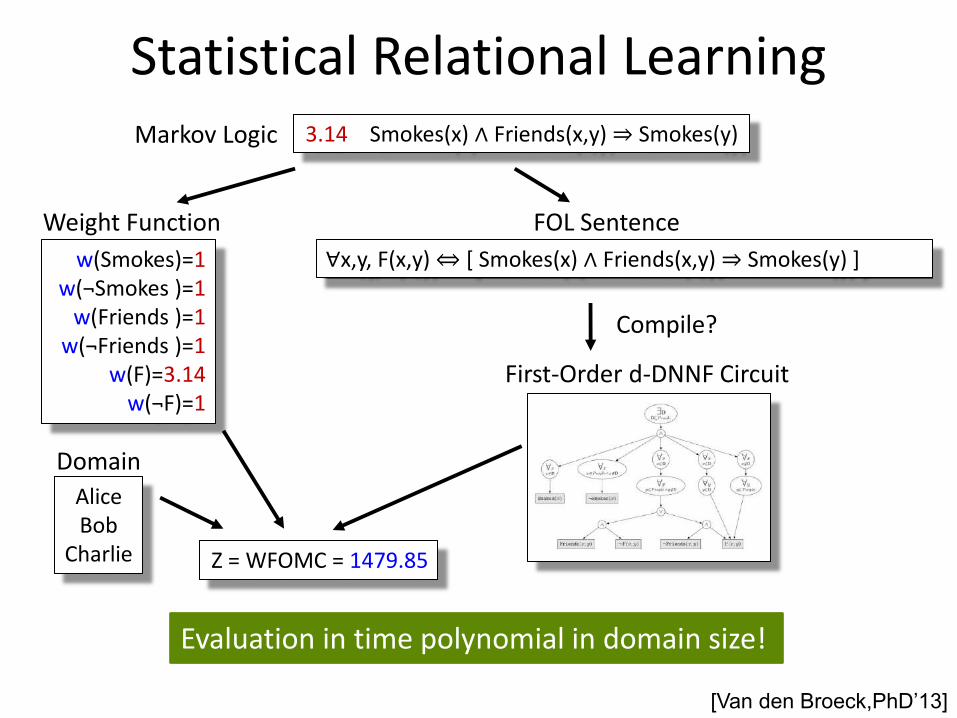
Statistical Relational Learning
Evaluation in time polynomial in domain size!
3.14 Smokes(x) ∧ Friends(x,y) ⇒ Smokes(y)
∀x,y, F(x,y) ⇔ [ Smokes(x) ∧ Friends(x,y) ⇒ Smokes(y) ]
Weight Function
w(Smokes)=1 w(¬Smokes )=1 w(Friends )=1 w(¬Friends )=1
w(F)=3.14 w(¬F)=1
FOL Sentence
First-Order d-DNNF Circuit
Domain
Alice Bob
Charlie Z = WFOMC = 1479.85
Markov Logic
[Van den Broeck,PhD‟13]
Compile? Compile?
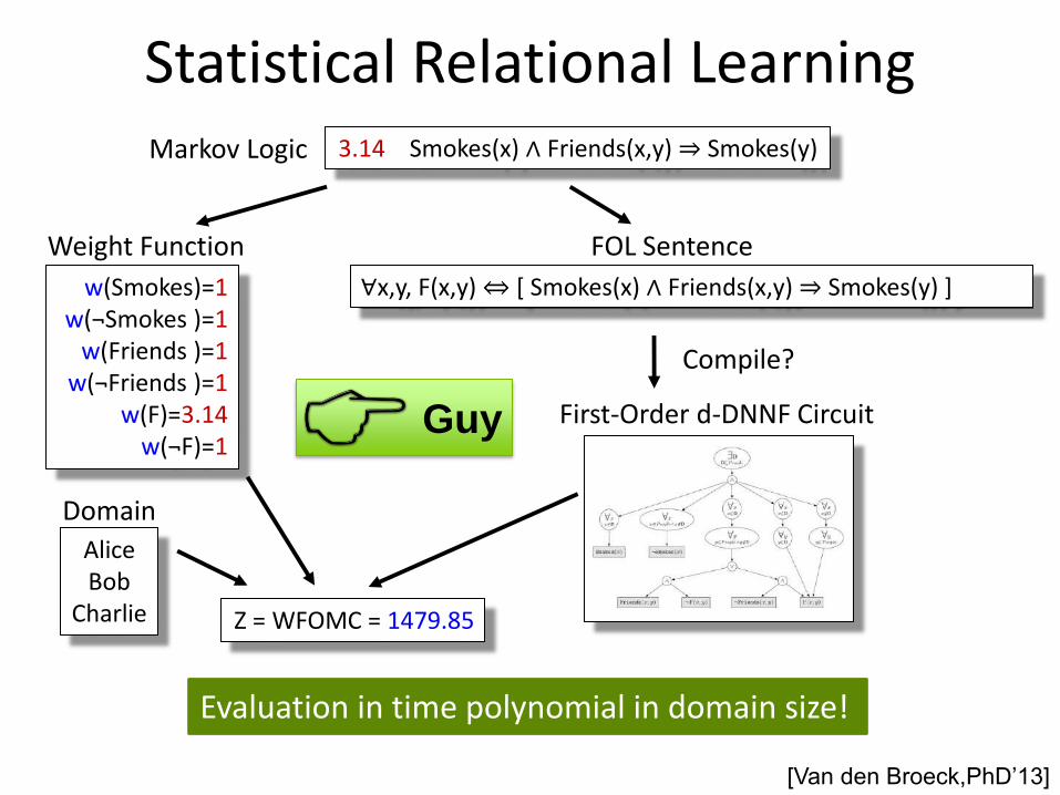
Statistical Relational Learning
Evaluation in time polynomial in domain size!
3.14 Smokes(x) ∧ Friends(x,y) ⇒ Smokes(y)
∀x,y, F(x,y) ⇔ [ Smokes(x) ∧ Friends(x,y) ⇒ Smokes(y) ]
Weight Function
w(Smokes)=1 w(¬Smokes )=1 w(Friends )=1 w(¬Friends )=1
w(F)=3.14 w(¬F)=1
FOL Sentence
First-Order d-DNNF Circuit
Domain
Alice Bob
Charlie Z = WFOMC = 1479.85
Markov Logic
[Van den Broeck,PhD‟13]
Compile? Compile?
Guy
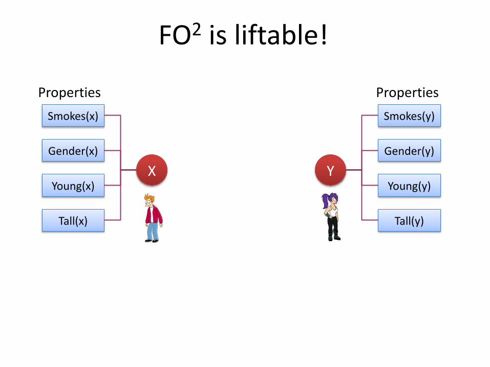
X Y
Smokes(x)
Gender(x)
Young(x)
Tall(x)
Smokes(y)
Gender(y)
Young(y)
Tall(y)
Properties Properties
FO2 is liftable!
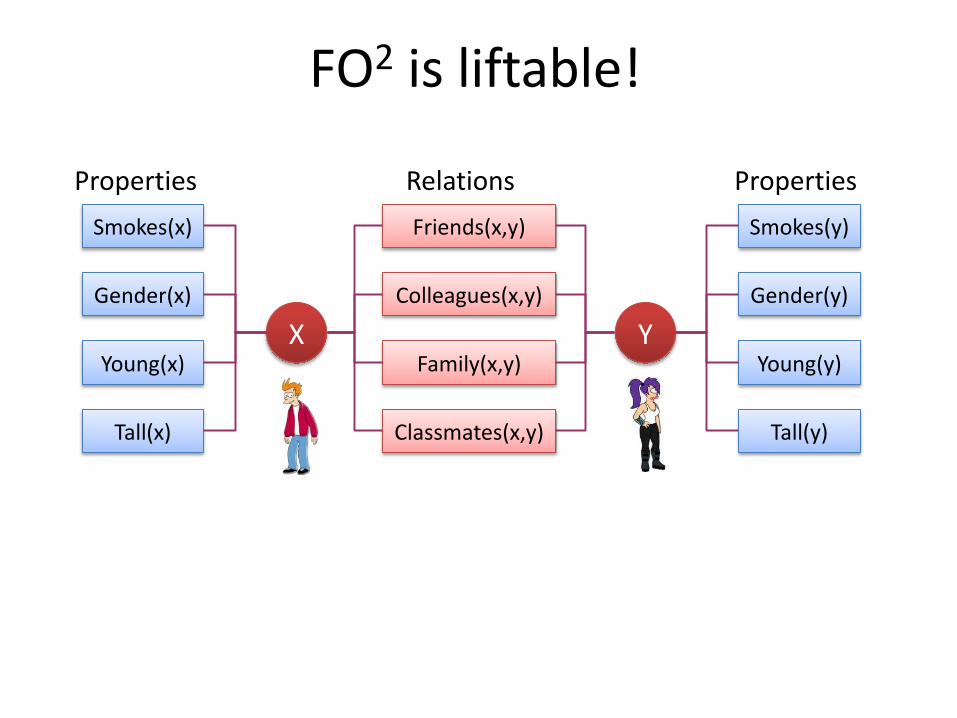
X Y
Smokes(x)
Gender(x)
Young(x)
Tall(x)
Smokes(y)
Gender(y)
Young(y)
Tall(y)
Properties Properties
Friends(x,y)
Colleagues(x,y)
Family(x,y)
Classmates(x,y)
Relations
FO2 is liftable!
X Y
Smokes(x)
Gender(x)
Young(x)
Tall(x)
Smokes(y)
Gender(y)
Young(y)
Tall(y)
Properties Properties
Friends(x,y)
Colleagues(x,y)
Family(x,y)
Classmates(x,y)
Relations
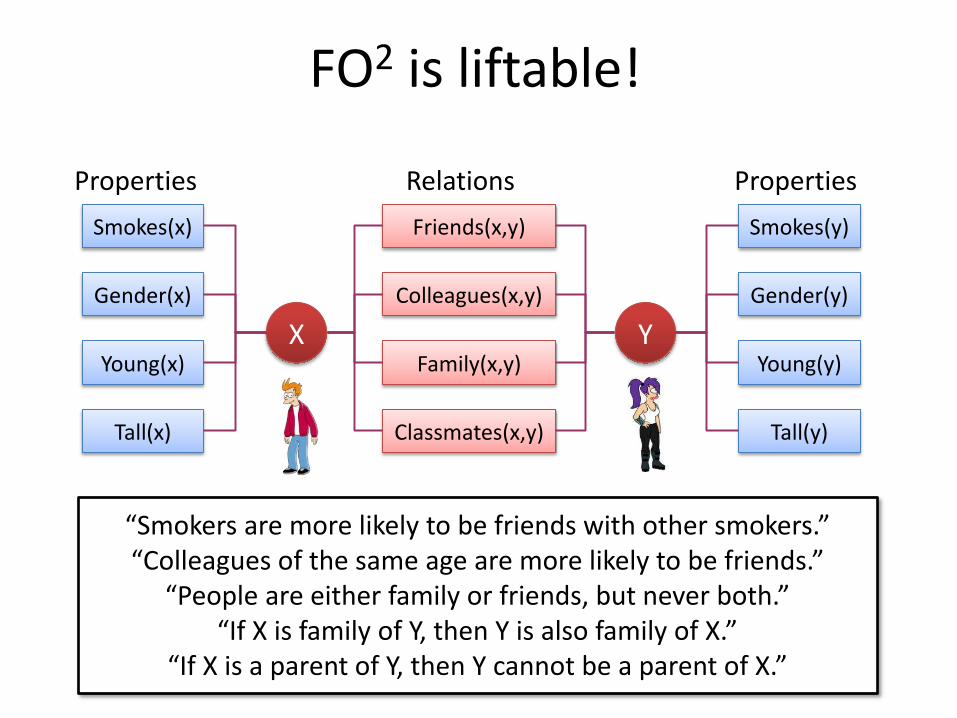
FO2 is liftable!
“Smokers are more likely to be friends with other smokers.” “Colleagues of the same age are more likely to be friends.”
“People are either family or friends, but never both.” “If X is family of Y, then Y is also family of X.”
“If X is a parent of Y, then Y cannot be a parent of X.”
More Pointers
• Lifted machine learning
• Open-world probabilistic databases
Guy
Guy
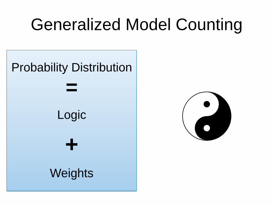
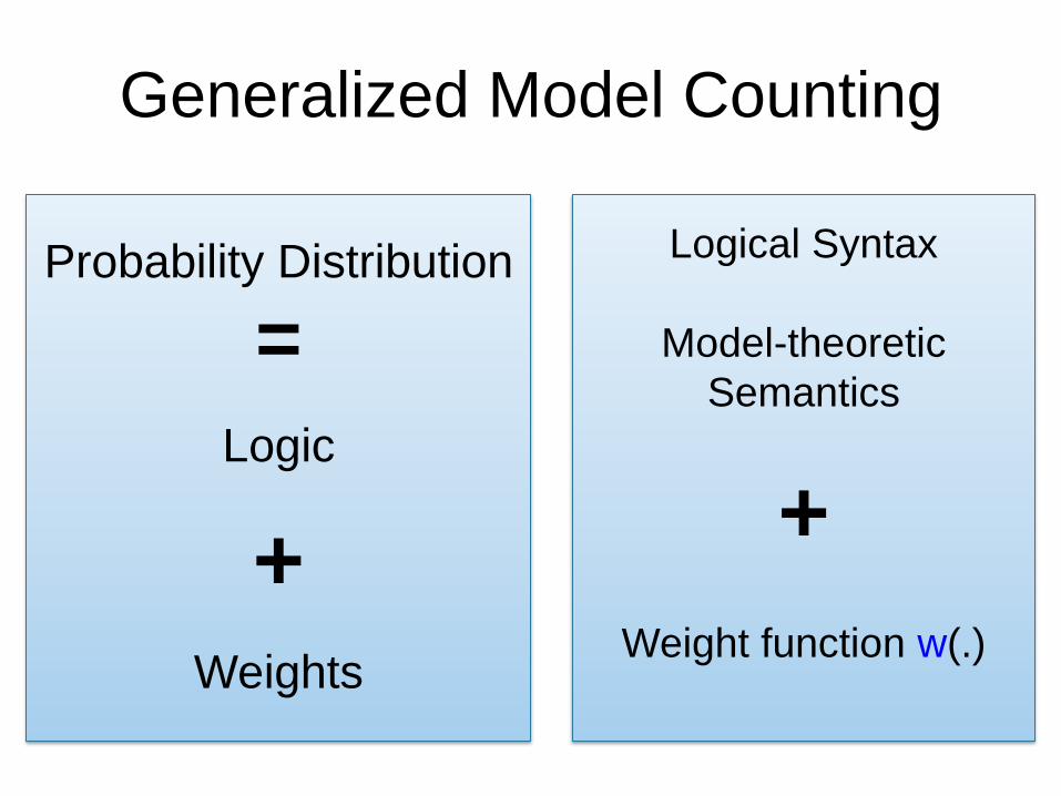
Generalized Model Counting
Probability Distribution
=
Logic
+
Weights
Generalized Model Counting
Probability Distribution
=
Logic
+
Weights
+
Logical Syntax
Model-theoretic
Semantics
Weight function w(.)
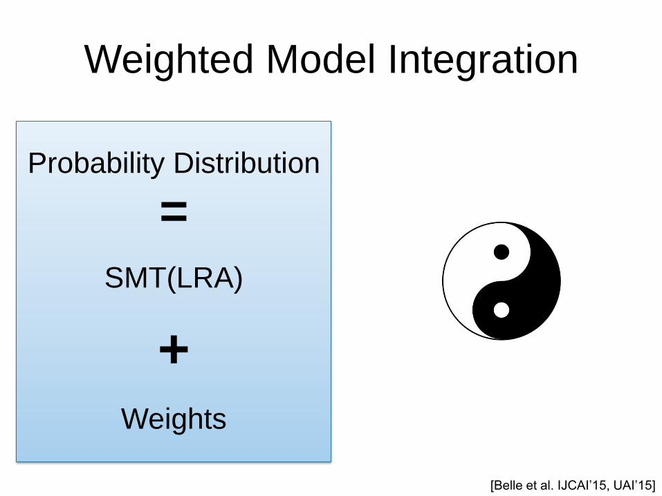
Weighted Model Integration
Probability Distribution
=
SMT(LRA)
+
Weights
[Belle et al. IJCAI‟15, UAI‟15]
Weighted Model Integration
Probability Distribution
=
SMT(LRA)
+
Weights
+
0 ≤ height ≤ 200
0 ≤ weight ≤ 200
0 ≤ age ≤ 100
age < 1 ⇒
height+weight ≤ 90
w(height))=height-10
w(¬height)=3*height2
w(¬weight)=5
…
[Belle et al. IJCAI‟15, UAI‟15]
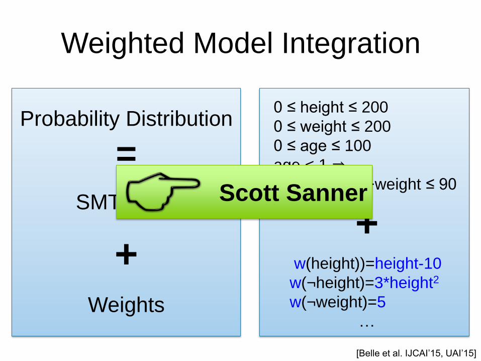
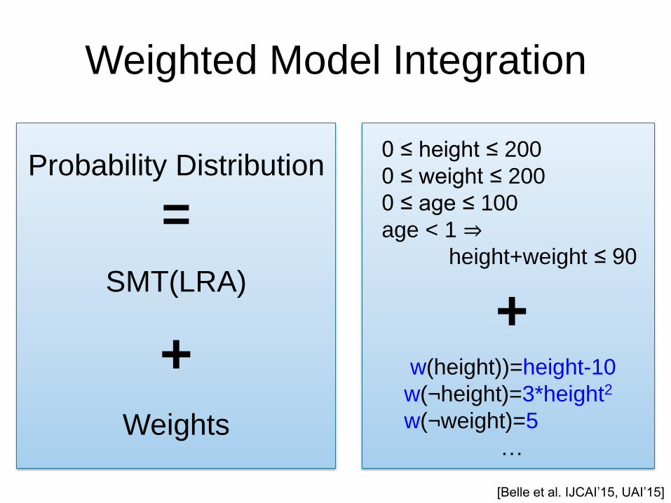
Weighted Model Integration
Probability Distribution
=
SMT(LRA)
+
Weights
+
0 ≤ height ≤ 200
0 ≤ weight ≤ 200
0 ≤ age ≤ 100
age < 1 ⇒
height+weight ≤ 90
w(height))=height-10
w(¬height)=3*height2
w(¬weight)=5
…
[Belle et al. IJCAI‟15, UAI‟15]
Scott Sanner
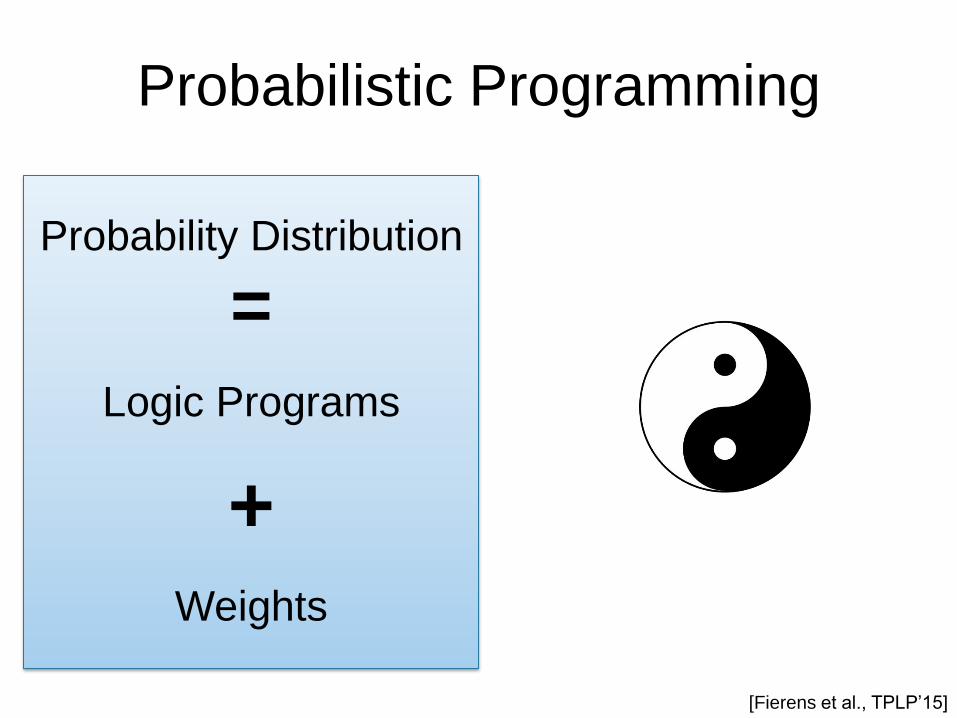
Probabilistic Programming
Probability Distribution
=
Logic Programs
+
Weights
[Fierens et al., TPLP‟15]
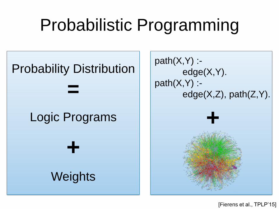
Probabilistic Programming
Probability Distribution
=
Logic Programs
+
Weights
+
path(X,Y) :-
edge(X,Y).
path(X,Y) :-
edge(X,Z), path(Z,Y).
[Fierens et al., TPLP‟15]
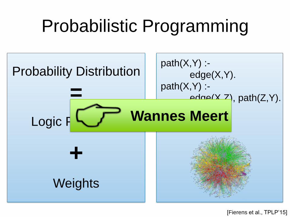
Probabilistic Programming
Probability Distribution
=
Logic Programs
+
Weights
+
path(X,Y) :-
edge(X,Y).
path(X,Y) :-
edge(X,Z), path(Z,Y).
[Fierens et al., TPLP‟15]
Wannes Meert
Conclusions
• Determinism and decomposability
generalize to first-order logic
• First-order model counting unifies
– Probabilistic databases
– High-level statistical AI models
• Fascinating computational complexity
questions
• Requires dedicated first-order solvers