FIRST-ORDER DRAFT IPCC WGII AR5 Chapter 21 Chapter · PDF fileInternational Financial...
97
FIRST-ORDER DRAFT IPCC WGII AR5 Chapter 21 Do Not Cite, Quote, or Distribute 1 11 June 2012 Chapter 21. Regional Context 1 2 Coordinating Lead Authors 3 Bruce Hewitson (South Africa), Anthony Janetos (USA) 4 5 Lead Authors 6 Timothy Carter (Finland), Filippo Giorgi (Italy), Richard Jones (UK), Won-Tae Kwon (Republic of Korea), Linda 7 Mearns (USA), Lisa Schipper (Sweden), Marten van Aalst (Netherlands) 8 9 Review Editors 10 Thomas Downing (USA), Phil Duffy (USA) 11 12 Volunteer Chapter Scientist 13 Kristin Kuntz-Duriseti (USA) 14 15 16 Contents 17 18 Executive Summary 19 20 21.1. Introduction 21 22 21.2. Defining Regions 23 21.2.1. Regional Manifestations of Climate Change 24 21.2.2. Regional Dimensions of Climate Change Response 25 26 21.3. Assessment of Methods of Regional Adaptation/Vulnerability/Assessment Literature 27 21.3.1. Decision-Making Context 28 21.3.1.1. Policy or Decision-Making Context 29 21.3.1.2. Consideration of Adaptation Approaches, Options, Possible Decisions, Adaptive 30 Capacity, Constraints 31 21.3.1.3. Time Scales of Interest 32 21.3.1.4. Spatial Scales of Interest 33 21.3.1.5. Sectors of Particular Interest 34 21.3.2. Baseline Information and Context – Current State and Recent Trends 35 21.3.2.1. Climate Baselines 36 21.3.2.2. Non-Climatic Baselines 37 21.3.3. Characterizing the Future 38 21.3.3.1. Development of Scenarios and Projections 39 21.3.3.2. Multiple Stressors 40 21.3.3.3. Application of Projections and Scenarios 41 21.3.4. Information Credibility and Uncertainty 42 21.3.4.1. Baseline Data 43 21.3.4.2. Uncertainties Regarding Future Climate 44 45 21.4. New Understanding and Emerging Knowledge on Climate Change 46 21.4.1. Physical Science Research 47 21.4.1.1. Atmosphere and Land Surface 48 21.4.1.2. Oceans and Sea Level 49 21.4.1.3. Air Quality 50 21.4.1.4. Cryosphere 51 21.4.2. Mitigation Research 52 21.4.2.1. Projections of Land-Use Change and Biofuels 53 21.4.2.2. Regional Aspects of Evolution of Technologies 54
-
Upload
doannguyet -
Category
Documents
-
view
214 -
download
0
Transcript of FIRST-ORDER DRAFT IPCC WGII AR5 Chapter 21 Chapter · PDF fileInternational Financial...

FIRST-ORDER DRAFT IPCC WGII AR5 Chapter 21
Do Not Cite, Quote, or Distribute 1 11 June 2012
Chapter 21. Regional Context 1 2 Coordinating Lead Authors 3 Bruce Hewitson (South Africa), Anthony Janetos (USA) 4 5 Lead Authors 6 Timothy Carter (Finland), Filippo Giorgi (Italy), Richard Jones (UK), Won-Tae Kwon (Republic of Korea), Linda 7 Mearns (USA), Lisa Schipper (Sweden), Marten van Aalst (Netherlands) 8 9 Review Editors 10 Thomas Downing (USA), Phil Duffy (USA) 11 12 Volunteer Chapter Scientist 13 Kristin Kuntz-Duriseti (USA) 14 15 16 Contents 17 18 Executive Summary 19 20 21.1. Introduction 21 22 21.2. Defining Regions 23
21.2.1. Regional Manifestations of Climate Change 24 21.2.2. Regional Dimensions of Climate Change Response 25
26 21.3. Assessment of Methods of Regional Adaptation/Vulnerability/Assessment Literature 27
21.3.1. Decision-Making Context 28 21.3.1.1. Policy or Decision-Making Context 29 21.3.1.2. Consideration of Adaptation Approaches, Options, Possible Decisions, Adaptive 30
Capacity, Constraints 31 21.3.1.3. Time Scales of Interest 32 21.3.1.4. Spatial Scales of Interest 33 21.3.1.5. Sectors of Particular Interest 34
21.3.2. Baseline Information and Context – Current State and Recent Trends 35 21.3.2.1. Climate Baselines 36 21.3.2.2. Non-Climatic Baselines 37
21.3.3. Characterizing the Future 38 21.3.3.1. Development of Scenarios and Projections 39 21.3.3.2. Multiple Stressors 40 21.3.3.3. Application of Projections and Scenarios 41
21.3.4. Information Credibility and Uncertainty 42 21.3.4.1. Baseline Data 43 21.3.4.2. Uncertainties Regarding Future Climate 44
45 21.4. New Understanding and Emerging Knowledge on Climate Change 46
21.4.1. Physical Science Research 47 21.4.1.1. Atmosphere and Land Surface 48 21.4.1.2. Oceans and Sea Level 49 21.4.1.3. Air Quality 50 21.4.1.4. Cryosphere 51
21.4.2. Mitigation Research 52 21.4.2.1. Projections of Land-Use Change and Biofuels 53 21.4.2.2. Regional Aspects of Evolution of Technologies 54

FIRST-ORDER DRAFT IPCC WGII AR5 Chapter 21
Do Not Cite, Quote, or Distribute 2 11 June 2012
21.4.2.3. Socioeconomic and Development Pathways 1 21.4.3. Approaches to Deriving Robust Information on Regional Change 2
3 21.5. Regional Distributions of Key Issues 4
21.5.1. Vulnerabilities 5 21.5.1.1. Methodological Issues 6 21.5.1.2. Regional Distribution 7
21.5.2. Impacts 8 21.5.2.1. Methodological Issues 9 21.5.2.2. Regional Issues 10
21.5.3. Adaptation Approaches 11 21.5.3.1. Methodological Issues 12 21.5.3.2. Regional Issues 13
21.5.4. Sectoral Issues 14 15 21.6. Cross-Regional Phenomena 16
21.6.1. Trade and Financial Flows 17 21.6.1.1. International Trade and Emissions 18 21.6.1.2. Trade and Financial Flows as Factors Influencing Vulnerability 19 21.6.1.3. Sensitivity of International Trade to Climate 20 21.6.1.4. International Financial Mechanisms as Instruments of Regional Climate Policy 21
21.6.2. Human Migration 22 21.6.3. Migration of Natural Ecosystems 23
24 21.7. Knowledge Gaps and Research Needs 25 26 Frequently Asked Questions 27 28 References 29 30 31 Executive Summary 32 33 [PLACEHOLDER FOR SECOND ORDER DRAFT: the text of the executive summary is preliminary pending the 34 addition of information from the FOD version of other WGII chapters, and updates from the WG I SOD, especially 35 where dependent on the completion of the CMIP5 archive] 36 37 Chapter 21 forms a juncture in the WGII report that comes between the thematic and conceptual chapters of part A 38 and the more detailed regional chapters impart B. In addition this chapter provides an interface with the relevant 39 regional messages found in WG I and WG III. The chapter provides an assessment for the practical application and 40 translation of information into a regional context. 41 42 43 Context of Regions 44 45 The dilemma faced in past assessments is that the most effective treatment of regional aspects of the observed and 46 projected physical climate, and its impacts and response options, may frequently be at odds with the scales at which 47 political decisions need to be made. Climate change transcends political boundaries and is highly variable from 48 region to region in terms of impacts and vulnerability. Likewise adaptation policies, options, and mitigation 49 strategies are strongly region dependent and tied to local and regional development issues. 50 51 Consequently a regional treatment is integral and essential for a proper understanding of climate and the cross-scale 52 issues. This chapter assesses a range of issues that act in concert with the climate at the regional scale, and include: 53

FIRST-ORDER DRAFT IPCC WGII AR5 Chapter 21
Do Not Cite, Quote, or Distribute 3 11 June 2012
• large scale components of the climate system with regional consequence such as the cryosphere, oceans, 1 sea level, and atmospheric composition 2
• climate change impacts on natural resource sectors, with regional contrasts in environmental conditions, 3 and the livelihoods and human interventions that accompany them, 4
• emissions of greenhouse gases and aerosols and the regional expression of their sources and sinks, 5 • global scenarios of the major socio-economic, technological and land use drivers that affect anthropogenic 6
emissions and also influence societal vulnerability at regional units of relevance to stakeholders wishing to 7 interpret and apply them, and 8
• human responses to climate change through mitigation and adaptation at multiple levels of governance. 9 10 At regional scales policy makers face a dual challenge in achieving policy integration – vertically, at multiple 11 administrative scales from global through national to local (multi-level governance), and horizontally, across 12 different sectors (policy coherence). They must also navigate through myriad existing political structures and 13 groupings (e.g. represented by the UNFCCC, regional, national and sub-national institutions). However, there are 14 also emerging challenges for international policy making that may not be covered adequately by current 15 international legal and humanitarian mechanisms, such as the opening up of the Arctic region, and environmental 16 migration. 17 18 Likewise, cross-regional phenomena can be crucial for understanding the ramifications of climate change at regional 19 scales, and its impacts and policies of response. These include global trade and international financial transactions, 20 which are linked to climate change through a number of pathways: (i) as a direct or indirect cause of anthropogenic 21 emissions, (ii) as a predisposing factor for regional vulnerability to the impacts of climate change, (iii) through their 22 sensitivity to climate trends and extreme climate events, and (iv) as an instrument for implementing mitigation and 23 adaptation policies. Migration is also a cross-regional phenomenon, whether of people or of ecosystems, both 24 requiring trans-boundary consideration of their causes, implications and possible interventions to alleviate human 25 suffering and promote biodiversity. 26 27 28 Baselines 29 30 The information used to establish the reference state for a system, and provide a baseline for calculating impacts 31 must account for the variability of the factors influencing the system. In the case of climate factors at least 30 years 32 of information, and often substantially more, is considered necessary. This includes baselines on variability over 33 timescales of days to decades. When defining baselines a wide range of information is required as the systems being 34 studied generally comprise interacting physical and human components influenced by climatic and non-climatic 35 factors. 36 37 Significant improvements have been made in the amount and quality of climate data that are available for 38 establishing reference states of climate-sensitive systems. These include new and improved observational datasets, 39 rescue and digitisation of historical datasets, and a range of improved global reconstructions of weather sequences 40 over past decades, in one case going back to 1880. Downscaling of coarse resolution global climate reconstructions 41 and models can provide information which gets closer to the temporal and spatial resolution requirements for 42 assessing vulnerability in many systems. Coordination of the assessment of this information is in its early days with 43 initial results indicating models can have significant errors in their high resolution reconstructions of the current 44 climate. Overall, the uncertainties inherent in model projections of regional climate changes have not decreased 45 from AR4; in some cases, the addition of regional forcings (e.g. topography) have increased some uncertainties. 46 47 Non-climatic factors relevant to assessing a system’s vulnerability general involve a complex mix of physical and 48 socio-economic influences. Often these are continually evolving and thus generally only a reference point in time 49 rather than a reference state over a period of time can be defined. There is significant new information on many of 50 the physical non-climatic factors, especially those which are components of the new RCPs used in the CMIP5. 51 Improvements in observations of other factors have also occurred but, as with climate information, in many cases 52 the quality is regionally dependent and there are resolution deficiencies. The literature on characterizing 53

FIRST-ORDER DRAFT IPCC WGII AR5 Chapter 21
Do Not Cite, Quote, or Distribute 4 11 June 2012
vulnerability on sub-national and regional scales is mixed – but it is clear that there is significant variation in 1 vulnerability due to variability in wealth, income, social factors, and access to governance. 2 3 4 Characterizing Future Change 5 6 The new developments subsequent to the AR4 relate principally to higher resolution climate scenarios, use of 7 multiple scenario elements that go further than only climate change scenarios, and a new approach to constructing 8 global scenarios as initiated by the development of representative concentration pathways (RCPs). 9 10 Projections of the future climate changes remain rooted in the GCM simulations, with studies dominantly still using 11 the CMIP3 generation of GCMs for impacts and adaptation studies. The data from CMIP5 has yet to be widely 12 adopted. Likewise, the downscaling to regional and high resolution still largely uses CMIP3, although significant 13 new initiatives are underway based on CMIP5. Important uncertainties remain in their application in impacts and 14 adaptation studies, as there continues to be a paucity of information on the relative merits and choice of different 15 methods available for generating high resolution data. 16 17 The expanded use of multiple scenario elements beyond that of only climate scenarios still has unresolved issues. 18 Among these are the downscaling of scenario elements, for example the economic activity information of RCPs, and 19 the possibly inconsistencies introduced in using local sources for some scenario elements. 20 21 The advent of the RCPs likewise opens new territory; both the TAR and AR4 assessments were based around SRES. 22 Whilst the RCPs embrace the range of scenarios found in the literature, they also include elements missing from the 23 SRES set. Likewise, the current development of the Shared Socio-economic Pathways (SSPs) characterize a wide 24 range of development pathways. However, at this stage of the AR5 most of the literature assessed for WG II remains 25 based on SRES. 26 27 Increased attention is being placed on the role of multiple stressors in the number of studies, with many having a 28 local or regional scope. This development has increased the need for a much wider range of data and wider range of 29 projections for the wide range of stressors, across multiple spatial scales. 30 31 As impacts and adaptation studies have progressed, more applications of projections and scenarios to actual 32 adaptation planning has occurred. Part of this development includes an increase in the number of scenarios used 33 from global or downscaled models, either through by using more models or using ensembles of a set of models to 34 explore the distribution of future impacts. 35 36 37 Credibility and Uncertainty of Information 38 39 For baseline information significant effort has been expended since the AR4 in improving the quality and 40 homogeneity of climate observations. This work allows for a more accurate quantification of the amplitude of 41 natural variability important for detecting trends or establishing impacts or vulnerability baselines. Complementing 42 these developments are the availability of new and enhanced global reanalyses. The availability of multiple 43 reanalyses further allows for the estimate of their uncertainty. Nonetheless, from the perspective of resolution, either 44 temporal or spatial, there are important credibility issues in some regions where significant biases remain. 45 46 [Credibility and uncertainty of non-climatic baseline data is a placeholder pending material from WG3 and other 47 WG2 chapter FODs] 48 49 Uncertainties of future climate remain centred on uncertainties over future climate forcing from emissions and 50 concentrations, the climate system response to forcing, and the natural internal variability of the climate system. The 51 likelihood of reducing uncertainty in future emissions and concentrations appears low, and future scenarios are 52 mainly presented as having equal plausibility. Uncertainty in the climate system uncertainty has multiple sources in 53 constrained understanding of the system dynamics, in how the system components are modelled, and in the 54
FIRST-ORDER DRAFT IPCC WGII AR5 Chapter 21
Do Not Cite, Quote, or Distribute 5 11 June 2012
parameterization of processes. Models are now more sophisticated that at the time of the AR4, and are more 1 complete in the components of the climate system that are included. Nonetheless, important processes remain 2 incomplete, for example the explicit modelling of ice sheet dynamics. 3 4 The models produce a range of projected futures, and for some variables and locations the sign of projected change 5 may differ from one model to another. However, in many instances this indicates a lack of significant change 6 compared to the natural variability for that region. The degree to which the model uncertainty can be reduced 7 remains an issue. [to be discussed in more detail by WG I SOD and WG I FAQ] 8 9 The role of natural variability as a source of uncertainty is important as a function of the time horizon being 10 considered and the spatial scale of interest. Recent work with large numbers of ensemble members has improved 11 measures of natural variability. 12 13 [Credibility of scenario elements will be addressed in the SOD] 14 15 16 New Understanding on Climate Change: Physical System 17 18 Regional climate information in the AR4 were not comprehensive enough to provide a coherent picture of past and 19 future regional changes with associated uncertainties. Improved regional scale information is now available. In 20 addition, more targeted analysis of climate projections for impact assessment studies have been carried out. The 21 leading messages from these developments include: [To be updated and developed after the WGI SOD] 22
• A strong regional variability of projected change is found for surface climate variables. Different indexes 23 combining sets of climate variables and statistics indicate the emergence of various climate change hot-24 spots at different times in the future. Better process understanding is needed to increase confidence in the 25 identification of climate change hot-spots. 26
• Broad regional patterns of late 21st century temperature and precipitation change projections, as well as 27 changes in temperature and precipitation extremes, from the latest generation GCM simulations (CMIP5) 28 are generally in line with previous projections available in the AR4. 29
• Preliminary analysis of decadal prediction experiments in the CMIP5 ensemble show that decadal 30 predictability of unforced regional precipitation and temperature patterns over land is very low. Indications 31 of some predictability of ocean temperatures of up to 10 years lead time is however found over some ocean 32 basins 33
• Uncertainties and ranges of regional scale projections have not decreased from the AR4, in fact the effects 34 of local forcings which can be represented with downscaling methods likely lead to an increase in 35 uncertainties. 36
• A larger set of global and regional (both dynamical and statistical) model projections allow a better 37 characterization of uncertainties than in the AR4, and more methods are available to produce probabilistic 38 projections of changes for use in IAV assessment work. 39
• Projected changes in the oceans, sea level and cryosphere are also consistent, at least qualitatively, with 40 previous estimates from the AR4 and with improved observations of recent past trends. Quantitative values 41 of projected changes may however differ from the AR4 due to the availability of better models and larger 42 ensembles, especially at the regional scale. 43
• Climate change is expected to substantially affect regional air quality, for example near surface ozone 44 concentrations, however this effect also depends strongly on future emissions. 45
46 The regional specifics of these are explored in the chapter under section 21.4.1 and considers both large scale 47 features processes, and continental scale assessment. 48 49 [To be updated and expanded when CMIP5 and CORDEX results become more available] 50 51 52 53

FIRST-ORDER DRAFT IPCC WGII AR5 Chapter 21
Do Not Cite, Quote, or Distribute 6 11 June 2012
New Understanding on Climate Change: Mitigation 1 2 The derivation of the RCP’s and the parallel process for scenario development has enabled the climate modeling 3 community to consider explicit mitigation scenarios for the first time. Substantial regional information (0.5 degree 4 global resolution) of economic activity, development trajectories, and emissions are available for analysis, but 5 remain largely unexplored. The RCP’s are known not to be unique pathways to the identified radiative forcing 6 targets. Model to model variability of the IAM’s used to generate the RCP’s is also largely unexplored. 7 8 The importance of land-cover and land-use changes as an indirect response to meeting mitigation targets has been 9 explored extensively since AR4. It is now clear that achieving targets without putting a price on carbon emissions 10 from land-use has the potential to lead to very large reductions in forested area, and much higher overall costs for 11 mitigation, compared to meeting the same targets while putting a price on all carbon emissions. Similarly, while 12 substantial regional variation in the availability of technologies is known to exist, the differences in how these are 13 represented regionally is largely unexplored. 14 15 A process (shared socioeconomic pathways, SSP’s) has been initiated to identify shared assumptions and global 16 scenarios for use in both mitigation and adaptation research. But although progress has been made, the vast majority 17 of the impacts, adaptation, and vulnerability literature since AR4 continues to be based on the SRES. 18 19 20 Cross-Regional Phenomena 21 22 The variability of vulnerability across regions, and across subpopulations within regions is an area of active 23 research, but methodological difficulties preclude general statements about the factors that control that variability, 24 and how they might evolve in the future. 25 26 Trade and financial flows influence both vulnerability and adaptive capacity, and also the regionalization of 27 emissions. At the same time, international and cross-regional financial instruments are being used to attempt to build 28 adaptive capacity as well as mitigation capacity. 29 30 Human migration in reaction to climate-driven phenomena, or extreme weather events, is usually within nations, but 31 under some circumstances, can extend across nations. The migration of ecosystems in response to changes in 32 climate emphasizes the need for cross-regional cooperation of conservation and resource management institutions. 33 34 35 21.1. Introduction 36 37 This chapter has several goals that play a new role in the IPCC scientific assessments. It seeks to highlight how the 38 thematic content of the first half of the volume has substantial regional variation and context, how regional 39 differences compare to each other, and what issues transcend regional boundaries. It then sheds light on how those 40 differences affect risk profiles, discusses the relevant outcomes of Working Groups’s I & III, and assesses regional 41 information about both non-climate Earth systems and the physical climate system. 42 43 To address these goals, the chapter focuses on four objectives: 44
1) It begins to identify the resources and regions that are subject to climatic risk, and identify the factors that 45 contribute to different levels of intrinsic vulnerability, from decision-making institutions to baseline 46 information and trends. The chapter summarizes the main features of commonality and differences among 47 regions, and explores methodological concerns with how regions are identified, how we understand the 48 different scales of regional decision-making, and which sectors are of particular interest, either because 49 they are common across regions, or because their variation across regions is especially important. 50
2) It articulates the exposure factors of risk – what is our current understanding of how we represent global 51 climate and its changes in regional terms – how do we do this for both climate trends and extremes, and 52 how well do we understand the extent to which regional changes in baselines can be attributed to 53 anthropogenic change. 54

FIRST-ORDER DRAFT IPCC WGII AR5 Chapter 21
Do Not Cite, Quote, or Distribute 7 11 June 2012
3) It explores how regional stakeholders and institutions can think concretely about characterizing the future 1 evolution of risk, so that the best science can be brought to bear on how that risk can be managed. 2 Therefore, the chapter presents its best judgment on the science behind the challenge of regionalizing 3 climate model output, and also on the science behind how regions would evolve in the absence of those 4 risks, and how they would respond to different adaptation and mitigation actions. 5
4) It explores the connections between regions, both in terms of their underlying baseline conditions, in how 6 they resemble or differ from each other, and in terms of how they affect each other through a range of other 7 drivers – trade, economic development, use of natural resources, and so on. So it is also a place within the 8 volume in which some degree of synthesis can be accomplished, in addition to its challenge to compare and 9 contrast regional contexts. 10
11 12 21.2. Defining Regions 13 14 The climate system may be global in extent, but its manifestations – through atmospheric processes, ocean 15 circulation, bioclimatic zones, daily weather and longer-term climate trends – are assuredly local in their occurrence, 16 character and impact. Explicit recognition of geographical diversity is therefore an imperative for any scientific 17 assessment of anthropogenic climate change. Regional heterogeneity is also a fundamental consideration in 18 designing appropriate policies for managing the challenges of climate change. The following sections emphasize 19 some of the crucial regional issues to be pursued in Part B of this report. 20 21 22 21.2.1. Regional Manifestations of Climate Change 23 24 Climate change respects no political boundaries and can be highly variable from region to region, regardless of 25 whether it is anthropogenic or natural in origin. Similarly, the impacts of climate change, the vulnerability of 26 different socio-economic sectors and the availability of adaptation policies are strongly region-specific. Finally, the 27 formulation of mitigation strategies and the implementation of mitigation technologies are intimately related to 28 local/regional development issues. The most effective treatment of regional aspects of the observed and projected 29 physical climate, its impacts and response options may frequently be at odds with the scales at which political 30 decisions need to be made. This has been the dilemma facing IPCC author teams in successive assessments. Some of 31 their earlier attempts at reconciling this mismatch have been summarized in Box 21-1. 32 33 _____ START BOX 21-1 HERE _____ 34 35 Box 21-1. Treatment of Regions in Previous IPCC Reports 36 37 There has been an evolution in the treatment of regional aspects of climate change in IPCC reports from a patchwork 38 of case examples in the First Assessment Report (FAR) and its supplements, through to attempts at a more 39 systematic coverage of regional issues following a request from governments, beginning with the Special Report on 40 the Regional Impacts of Climate Change in 1998. That report distilled information from the Second Assessment 41 Report (SAR) for ten continental scale regions, and the subsequent Third (TAR) and Fourth (AR4) assessments each 42 contained comparable chapters on impacts, adaptation and vulnerability in the Working Group (WG) II volumes. 43 WG I and III reports also address regional issues in various chapters, and use different methods of mapping, 44 statistical aggregation and spatial averaging to provide regional information. Examples of past attempts to represent 45 regional information are presented in Table 21-1. Some of the main topics demanding a regional treatment are: 46
• Climate, typically represented by sub-continental regions, a scale at which trends in observations tend to be 47 fairly robust, and at which signal:noise ratios for projections from global models may also offer some 48 confidence. While maps are widely used to represent climatic patterns, regional aggregation of this 49 (typically gridded) information is still required to summarise the processes and trends they depict. Indeed, 50 examples of maps produced for an atlas accompanying the WG I report can be found in several regional 51 chapters of this volume. Figure 21-1 illustrates how sub-continental land-based regions being used to 52 summarise observed and projected climate map onto the regions defined by chapters in Part B. Specific 53

FIRST-ORDER DRAFT IPCC WGII AR5 Chapter 21
Do Not Cite, Quote, or Distribute 8 11 June 2012
examples of summary climate information that can be provided at sub-continental scales directly applicable 1 to political regions are provided in Box 21-3. 2
• Other aspects of the climate system, such as the cryosphere, oceans, sea level, and atmospheric 3 composition, also invite a regional treatment, especially given the importance of regional changes, for 4 example, in sea ice cover for navigation, land movements and local circulations that may counter or 5 reinforce global sea level rise, or air pollution that can be a major regional driver of atmospheric radiative 6 forcing. 7
• Climate change impacts on natural resource sectors, such as agriculture, forestry, ecosystems, water 8 resources and fisheries, which often demand a classification of regional types to distinguish contrasting 9 environmental conditions, and the livelihoods and human interventions that accompany them. Here, it is 10 common to classify regions according to biogeographical characteristics (e.g. biomes, climatic zones, 11 physiographic features like mountains, river basins or deltas, or combinations of these). 12
• Emissions of greenhouse gases and aerosols and their cycling through the Earth system have a crucial 13 regional expression that requires combining socio-economic data on human activities responsible for 14 anthropogenic emissions with biogeochemical monitoring of material and gas fluxes worldwide. Since 15 these activities are known to be responsible for anthropogenic climate change, and the UNFCCC and other 16 national and international policies are being designed to modify human activities, the regional units of most 17 relevance for governments are those that provide comparison between political and economic regional 18 groupings worldwide. 19
• Global scenarios of the major socio-economic, technological and land use drivers that affect anthropogenic 20 emissions as well as influencing societal vulnerability to the impacts of climate change, rely heavily on 21 integrated assessment models (IAMs) of the global energy–environment–socioeconomic system. IAMs 22 require historical statistical information from all regions of the world to establish relationships between key 23 driving variables and the observed behaviour of ecosystems, the climate system, energy systems, economic 24 activity and society at large. Quantitative scenarios derived from such models need to be aggregated into 25 regional units of relevance to stakeholders wishing to interpret and apply such scenarios. SRES was the 26 most comprehensive scenario development exercise conducted to date to serve the climate change 27 community, though the scenarios themselves are provided only for four world regions. New scenarios are 28 under development by the global research community, and these are being designed to have more regional 29 detail than SRES (Moss et al., 2010). 30
• Finally, human responses to climate change through mitigation and adaptation demand both global and 31 regional approaches, as emphasised in the Articles of the UNFCCC and manifest in international financing 32 to support climate policy (e.g. via the Multinational Development Banks – CIF, 2012). However, 33 governments require access to useable knowledge that can be applied at national and local scales. That is a 34 regional challenge beyond the scope of an IPCC report alone, but is something that all authors should have 35 in mind as the ultimate deliverable for which these assessments should provide the appropriate context. 36
37 _____ END BOX 21-1 HERE _____ 38 39 [INSERT TABLE 21-1 HERE 40 Table 21-1: Selected examples of regional treatment in previous IPCC Assessment Reports and Special Reports 41 (SR). Major assessments are subdivided by the three Working Group reports, each described by generic titles.] 42 43 [INSERT FIGURE 21-1 HERE 44 Figure 21-1: [PLACEHOLDER] Maps showing the 26 regions (land areas only) used to summarise projected 45 changes in climate in this chapter (upper panel – IPCC, 2012) and the regions defined for Chapters 22-29 in Part B 46 (lower panel – IPCC, 2001). Note that information is also provided in this chapter on projected climate over the 47 open oceans. [Maps to be redrawn and combined when climate regions and AR5 chapter regions clarified]] 48 49 50 21.2.2. Regional Dimensions of Climate Change Response 51 52 This is the first full IPCC assessment to devote a single part of a report to regional aspects of climate change that cut 53 across topics in all three IPCC Working Groups. Hence, the scope of the report includes all those regional 54
FIRST-ORDER DRAFT IPCC WGII AR5 Chapter 21
Do Not Cite, Quote, or Distribute 9 11 June 2012
dimensions of the climate change issue that are regarded as relevant to international policy making. Furthermore, as 1 the demand for information to support practical decision-making assumes an increasingly sub-national focus, this 2 can only accentuate the challenge facing the authors of this report. However, though expeditious use of case studies 3 can provide useful illustrations of local-scale phenomena, geographical comprehensiveness is necessarily ruled out 4 in an international assessment of this kind. Instead, responsibility for compiling and disseminating local information 5 rests with regional and national experts, and IPCC reports seek to highlight robust examples of these, wherever 6 possible. 7 8 In addition to scale issues, the implications of climate change also touch on almost all sectors of society, so policy 9 makers face a dual challenge in achieving policy integration – vertically, through multiple levels of governance, and 10 horizontally, across different sectors (Figure 21-2). Many of the barriers to effective climate response are to be 11 found in these two dimensions. For instance, in the vertical dimension, while a growing number of European 12 countries have developed national adaptation strategies in recent years, the implementation of adaptation measures 13 at a local level has lagged behind, because responsibility and resources for adaptation at the local level have yet to 14 be properly assigned (Biesbroek et al., 2010). In contrast, horizontal integration (policy coherence – Mickwitz, 15 2009) often flies in the face of conventional practice, with sectoral policies that are designed to advance social or 16 economic goals (e.g. development of an improved road network) often at odds with goals set in other sectors (e.g. 17 environmental targets to limit greenhouse gas emissions or to reduce infrastructural exposure to flood risk). 18 19 [INSERT FIGURE 21-2 HERE 20 Figure 21-2: Horizontal and vertical climate policy integration (Mickwitz et al. 2009). Vertical policy integration 21 can occur within as well as between levels, and may extend to supra-national and global levels (not shown). 22 [possibly redraw to include international dimensions]] 23 24 At the international level, the United Nations Framework Convention on Climate Change (UNFCCC) is explicit in 25 its definitions regarding the status and groupings of its signatories or "Parties" (UNFCCC, 1992). The principle of 26 "common but differentiated responsibilities" refers to a common goal of Parties to achieve the objective of the 27 Convention and to implement its provisions, while recognizing specific national and regional development priorities, 28 objectives and circumstances. The most fundamental distinction is drawn between the Annex I Parties, comprising 29 industrialized (developed) countries1, and the Non-Annex I Parties, which are mostly developing countries (Table 30 S21-2). Annex I OECD members are further designated as Annex II Parties. These Parties have special 31 responsibilities to provide financial assistance to developing countries as well as promoting the development and 32 transfer of environmentally friendly technologies to transition economy Parties and developing countries. All but 33 two of the Annex I Parties (Belarus and Turkey) also signed up to emissions limitations or reductions under the 34 Kyoto Protocol (Annex B – Table S21-2). Developing countries eligible to receive official development assistance 35 (ODA) are classified by the OECD according to per capita income. 48 of these are designated by the United Nations 36 as Least Developed Countries (LDCs)2, and are recognized under the Convention as meriting special consideration 37 on account of their limited capacity to respond to climate change and adapt to its adverse effects. 38 39 [INSERT TABLE S21-2 APPENDIX – SUPPLEMENTARY MATERIAL 40 Table S21-2: [Proposed that this be moved supplementary material] Countries and territories of the world, their 41 regional treatment in this report and some other illustrative groupings of relevance for international climate change 42 policy making. Sources (status in May 2012): AOSIS (2012), Arctic Council (2012), European Commission (2012), 43 G77 (2012), OECD (2012), OHRLLS (2012), OPEC (2012), Secretariat of the Antarctic Treaty (2012), UNCLOS 44 (2012), UNFCCC (1992, 1998, 2012). [If supplementary material, possibly to be used in conjunction with an 45 interactive map and other statistical information, e.g. population, GDP, HDI?]] 46 47 [FOOTNOTE 1: Members of the Organisation for Economic Co-operation and Development (OECD) in 1992 plus 48 transition economies.] 49 50 [FOOTNOTE 2: LDC status is determined by the High Representative for the Least Developed Countries, 51 Landlocked Developing Countries and Small Island Developing States (OHRLLS) according to three criteria: gross 52 national per capita income (GNI), a composite human assets index (HAI), based on indicators of nutrition, health, 53 education and literacy, and an economic vulnerability index (EVI) based on seven economic indicators.] 54

FIRST-ORDER DRAFT IPCC WGII AR5 Chapter 21
Do Not Cite, Quote, or Distribute 10 11 June 2012
1 The Convention also contains descriptions of regional types without specifying which countries fall within these 2 categories. For example, Article 4 of the Convention describes the following regional types in relation to funding, 3 insurance and the transfer of technology: (a) small island countries; (b) countries with low-lying coastal areas; (c) 4 countries with arid and semi-arid areas, forested areas and areas liable to forest decay; (d) countries with areas prone 5 to natural disasters; (e) countries with areas liable to drought and desertification; (f) countries with areas of high 6 urban atmospheric pollution; (g) countries with areas with fragile ecosystems, including mountainous ecosystems; 7 (h) countries whose economies are highly dependent on income generated from the production, processing and 8 export, and/or on consumption of fossil fuels and associated energy-intensive products; and (i) landlocked and 9 transit countries. Two of these (Landlocked Developing Countries and Small Island Developing States) are 10 recognized by the United Nations Office of the High Representative for the Least Developed Countries (OHRLLS) 11 (see Table S21-2). 12 13 While the UNFCCC and its associated Protocols require global agreement to come into effect, the implementation of 14 policies to meet these agreements occurs at national level. Moreover, the negotiating process is often conducted 15 among regional groupings of nation states. Some examples are shown below (from past COP3 meetings): 16
• African Group 17 • Alliance of Small Island States (AOSIS – Table S21-2) 18 • Asian Group 19 • A group of countries of Central Asia, Caucasus, Albania and Moldova (CACAM) 20 • Environmental Integrity Group (EIG) comprises: Mexico, the Republic of Korea and Switzerland 21 • European Union (Table S21-2) 22 • Group of 77 and China4 (Table S21-2) 23 • OPEC (Organization of the Petroleum Exporting Countries – Table S21-2)5 24 • Umbrella group: a loose coalition of non-EU developed countries, usually comprising: Australia, Canada, 25
Iceland, Japan, New Zealand, Norway, the Russian Federation, Ukraine and the USA. 26 27 [FOOTNOTE 3: The Conference of the Parties (COP) comprises all Parties to the Convention and is its supreme 28 decision-making authority.] 29 30 [FOOTNOTE 4: The Group of 77 (G-77) was established on 15 June 1964 by seventy-seven developing country 31 signatories of the "Joint Declaration of the Seventy-Seven Countries" issued at the end of the first session of the 32 United Nations Conference on Trade and Development (UNCTAD). Although the membership of the G-77 has 33 increased to 130 countries, the original name was retained because of its historic significance.] 34 35 [FOOTNOTE 5: OPEC is an international organization of 12 developing countries that are heavily reliant on oil 36 revenues as their main source of income. Membership is open to any country which is a substantial net exporter of 37 oil and which shares the ideals of the organization.] 38 39 Many of the initiatives emerging out of the UNFCCC process, are focused on capacity building at national-scale 40 (e.g. the Nairobi Work Programme on Impacts, Vulnerability and Adaptation to Climate Change – (UNFCCC, 41 2007)) while the international financial mechanisms for implementation of response measures (e.g. the Clean 42 Development Mechanism for emissions reductions under the Kyoto Protocol (UNFCCC, 1998), or the Green 43 Climate Fund to support adaptation actions under the Convention (Green Climate Fund, 2012)) are administered by 44 committees drawn from different regional groupings. 45 46 It is also becoming clear that as climate change impacts become felt in different regions, some existing international 47 institutional alignments are facing new challenges. For instance, the opening of new transport routes in the Arctic 48 (see section 21-6 and Chapter 28) coupled with new opportunities to exploit natural resources in the region and a 49 number of territorial disputes, have raised national security concerns that the existing laws governing access and 50 sovereignty may be too flimsy, and that institutions such as the Arctic Council may need to be strengthened to match 51 the unified legal framework already in place for the Antarctic under the Antarctic Treaty (Bergman Rosamond, 52 2011; Government Office for Science, 2011). However, although there is no single legally binding Arctic 53 environmental regime, there are already strong provisions within the United Nations Convention on the Law of the 54

FIRST-ORDER DRAFT IPCC WGII AR5 Chapter 21
Do Not Cite, Quote, or Distribute 11 11 June 2012
Sea (Stokke, 2007). Signatories of the Antarctic Treaty and UNCLOS, and members of the Arctic Council are 1 indicated in Table S21-1. Similar challenges face international authorities faced with large numbers of migrants, 2 some of whom are moving directly or indirectly as a result of envirinmental change (see Section 21.6.2). 3 4 Finally, as an interesting curiosity, but also to illustrate how international agreements can be used to promote 5 regional development, and hence might also be promising instruments for furthering trans-national aspects of 6 climate policy, it can be noted in Table S21-1 how a large number of UNCLOS signatories are actually Landlocked 7 Developing Countries (LLDCs). This is merely recognition that the Convention makesprovision for LLDCs and 8 other "geographically disadvantaged States" to participate in the equitable exploitation of resources in the exclusive 9 economic zones of coastal neighbours, as well as being guaranteed rights of access and tax-free transit via coastal 10 ports (UNCLOS, 1982). 11 12 13 21.3. Assessment of Methods of Regional Adaptation/Vulnerability/Assessment Literature 14 15 Assessing climate vulnerability or options for adapting to climate impacts in human and natural systems requires an 16 understanding of all factors influencing the system and how change may be effected within the system or applied to 17 one or more of the external influencing factors. This implies the need, in general, for a wide range of climate and 18 non-climate information and then determining how this may be used to enhance the resilience of the system. Firstly 19 in this section, the context in which systems operate and relevant knowledge can be applied is explored from which 20 a broad description of the information requirements can be deduced. This is followed by assessments of new sources 21 of, and thinking related to baseline and recent trend information necessary for defining impacts baselines and 22 assessing vulnerability and then the future scenario information used for assessing impacts, changes in vulnerability 23 and options for adaptation. The section concludes with an assessment of the credibility of the various types of 24 information presented. 25 26 27 21.3.1. Decision-Making Context 28 29 This section deals with understanding the different types of situation in which decisions related to the impacts of 30 climate change are being made, and what human and natural systems are involved. This understanding allows the 31 types of information required to be defined along with the characteristics of the quantities involved, such as the level 32 of spatial or temporal detail or measures of quality. 33 34 As discussed in the IPCC SREX (IPCC 2012), the selection of appropriate vulnerability and risk evaluation 35 approaches depends on the decision-making context. Different decision-making contexts lead to different choices of 36 climate variables and of the geographic and time scales on which they need to be provided. They also lead to 37 different ways to best characterize vulnerability, and in how to define and evaluate adaptation options, in the context 38 of uncertainty about not only the future climate, but also many other aspects of the system at risk. In addition, the 39 decision-making context also defines which assessment approach is most appropriate. Some decision-making 40 contexts, such as the design of large infrastructure projects, may require rigorous quantitative information to feed 41 formal evaluations, often including cost-benefit analysis. Others, such as local decision-making in traditional 42 communities, may benefit much more from experienced-based approaches, or story-telling to evaluate future 43 implications of possible decisions. In most cases, an understanding of the context in which the risk plays out, and the 44 “menu of options” that may be considered the manage it, are not an afterthought, but a defining feature of an 45 appropriate climate risk analysis, which requires a much closer interplay between decision-makers and providers of 46 climate risk information than is often occurring. 47 48 While the importance of considering the decision-making context is a general issue for all vulnerability, impacts and 49 adaptation assessments, it is of special importance in the context of regional and sub regional assessments. Many 50 studies are still driven by global data and methods, whereas there is considerable variation in regional, national and 51 local decision-making contexts, as well as across different groups of stakeholders and sectors. There is a growing 52 body of scientific information on how to provide the most relevant climate risk information to suit specific decision-53 making processes [add refs]. 54

FIRST-ORDER DRAFT IPCC WGII AR5 Chapter 21
Do Not Cite, Quote, or Distribute 12 11 June 2012
1 2 21.3.1.1. Policy or Decision-Making Context 3 4 The most defining characteristic of the decision-making context is by whom decision are being taken. This may 5 range from international policy processes, to national government departments, to individual farmers. 6 7 Historically, except for studies purely from a research perspective, many climate change risk assessments have been 8 undertaken either in the context of the UNFCCC, or by (or for) national governments. The purpose was often to 9 define the long-term international or national implications of climate change, to assess the priority that would need 10 to be given to climate change mitigation, or to assess long-term risks to specific countries, regions, and sectors. 11 Clearly, the level of current development, which often strongly relates to the size of the current “adaptation gap”, is 12 an important determinant in that level of vulnerability. Such differences in levels of development, as well as specific 13 regional geographic characteristics, continue to be an important component of regional differences in the climate 14 change adaptation policy-context. 15 16 As attention has shifted towards implementing adaptation, more and more attention is also being paid to more 17 sector-specific risk assessments intended to guide development planning and specific investments, by governments, 18 but also other actors in societies (e,g, add ref to UKCIP), including at the most local levels. 19 20 International organizations including the UN and its specialized agencies, as well as the World Bank and regional 21 development banks, have inreasingly sought to integrate climate risk management in their regular programs, and in 22 their support to (particularly developing country) governments. Many climate information sources initially started 23 globally but have increasingly been tailored to specific country circumstances (e.g. World Bank climate-adaptation 24 country profiles that aim to provide a more comprehensive assessement of country risk, UNDP country profiles, 25 focusing only on climate information). Documents such as the UN-DAF and the World Bank’s Country Assistance 26 Strategy increasingly aim to mainstream climate adaptation into their development assistance to individual 27 countries. Specifically climate-oriented investments, such as specific projects funded by international climate 28 financing mechanisms, also build on specific analyses of climate information, often carried out by the recipient 29 government with assistance from the international organization involved. 30 31 At regional and subregional scale, the climate adaptation decision-making context also includes a range of regional 32 intergovernmental organizations, from continental ones such as such as OAS, and the African Union, to sub 33 continental ones such as ECOWAS, IGAD and SADC within sub-Saharan Africa. Most of these organizations are 34 active on topics and in sectors that are significantly affected by climate risk, and many have developed climate 35 change related policies or plans [add examples?]. 36 37 Civil society organizations, ranging from international NGOs to local community-based organizations (CBOs), with 38 big differences in level of awareness and technical capacity to take climate risk into account into their activities (and 39 to integrate technical climate information into their adaptation work, to the extent relevant). Some, such as the Red 40 Cross and Red Crescent Movement and CARE international, have established dedicated units to build capacity for 41 climate risk management and related work, and to provide guidance on climate risk assessment and appropriate use 42 of climate information. 43 44 Another important category of users is the private sector, ranging from large multinationals to small local 45 enterprises and individual farmers. In most sectors, private sector use of climate information is often focused more 46 on the current and near-term climate (including what has already changed), except in the case of requirements to 47 include climate risk assessments in Environmental Impact Assessments, or in the case of large investments directly 48 affected by long-term trends in climate (with a long investment horizon and substantial exposure and vulnerability to 49 changing climate conditions). 50 51 Individuals are also affected by climate individually, by impacts on their livelihoods, well-being and health, 52 including through the direct impact of extreme events. 53 54

FIRST-ORDER DRAFT IPCC WGII AR5 Chapter 21
Do Not Cite, Quote, or Distribute 13 11 June 2012
Decision-making by individual, communities, and private companies significantly affects the adaptive capacity of 1 societies at large. To some extent, their decision-making is affected by the context of government policies and 2 legislation. However there are substantial regional and subregional differences in the way these individuals, 3 communities and the private sectors relate to the government, both in terms of the extent to which the government’s 4 policies affect private behavior, and the extent to which government information is trusted and acted upon and thus 5 results in behavioral change. In addition, there are significant regional and subregional differences in the extent to 6 which individuals, especially the most vulnerable, can influence government decision-making, which in itself is an 7 aspect of adaptive capacity. 8 9 10 21.3.1.2. Consideration of Adaptation Approaches, Options, Possible Decisions, Adaptive Capacity, Constraints 11 12 Another defining question is the approach to adaptation. If plans or projects are designed specifically to adapt to a 13 changing climate, climate risk information has quite a central role in the decision-making. Examples include 14 National Communications to the UNFCCC, NAPAs, SPCRs, but also climate change strategies developed by local 15 towns, by international organizations, etc. 16 17 More frequently however, climate change is being considered as a smaller component of a regular set of 18 considerations for a particular decision. Examples include government sector plans, a particular infrastructure 19 investment, or even the day-to-day decisions by a local farmer. In such a context, the question is not just what is the 20 best available climate information, but also whether that information is relevant given the nature of the decision 21 being taken, and the constraints faced by the actors involved. When framed as a risk management problem, the 22 question is also not just about the nature of the risk and the uncertainties about possible future conditions, but also 23 about relative costs and benefits of the “menu of options” available to manage that risk. 24 25 In many cases, climate change may merely provide an incentive for choosing a more robust strategy, which leaves 26 more flexibility for future risk management. In such contexts, the focus may shift from approaches to formally factor 27 in climate information in specific technical design decisions, to one where the emphasis is on building adaptive 28 capacity, and the analysis should primarily focus on capacities and constraints rather than technical climate analysis. 29 30 A particularly important aspect in cases where climate is only one of many factors (and thus risks being ignored) is 31 to avoid maladaptation, which may result from decisions taken unaware of potential changes in climate risk. As 32 highlighted in SREX (IPCC 2012), some decisions taken to manage short-term climate risk may result in 33 maladaptation in the longer term. 34 35 36 21.3.1.3. Time Scales of Interest 37 38 As stated in SREX (IPCC 2012), observed and projected trends in exposure, vulnerability, and climate can inform 39 risk management and adaptation strategies, policies, and measures, but the importance of these trends for decision 40 making depends on their magnitude and degree of certainty at the temporal and spatial scale of the risk being 41 managed, as well as on the available capacity to implement risk management options. 42 43 Many climate change impacts assessments have traditionally focused on the longer-range future (2050-2100), 44 whereas many decisions taken today have a planning horizon of a few months, years, maybe up to 2 decades. For 45 many such shorter-term decisions, adaptation to recent climate variability and observed trends may be sufficient 46 (Hallegatte 2009). In doing so, there is often scope to make better use of climate information on shorter timescales, 47 including better use of current climatologies and seasonal climate forecasts (HLT, 2011). For longer-term decisions, 48 questions about maladaptation, and sequencing of adaptation options become much more pertinent. 49 50 51 52

FIRST-ORDER DRAFT IPCC WGII AR5 Chapter 21
Do Not Cite, Quote, or Distribute 14 11 June 2012
21.3.1.4. Spatial Scales of Interest 1 2 A lot of climate change adaptation planning is still taking place at the national scale, partly due to the challenges 3 involved with the proper communication of relevant climate information at the local level (given both the 4 uncertainties involved and the mode of communication). However, as also noted in SREX (IPCC, 2012) better use 5 of local level risk and context analysis methodologies, increasingly accepted by many civil society and government 6 agencies working on adaptation at local level, could enhance climate risk management at multiple levels. 7 8 Decisionmaking for large-scale structural measures is often based on cost-benefit analyses and technical approaches. 9 Household-level (and many other local) climate-affected decisions, particularly those involving changing regular 10 practice or behavior, are often made much more intuitively, with a much greater role for a wide range of social and 11 cultural aspects. This poses very different demands on the type of climate information provided (see SREX Box 5-12 2). 13 14 Multi- criteria analysis, scenario planning, and flexible decision paths offer options for taking action when faced 15 with large uncertainties or incomplete information, and can help bridge adaptation strategies across scales (in 16 particular between the national and local level ) (SREX ch 5/6). 17 18 _____ START BOX 21-2 HERE _____ 19 20 Box 21-2. SREX-Derived Information on Communication of Local Risk-Based Information 21 22 [Placeholder – to be developed subject to materials from FOD in other WGII chapters] 23 24 _____ END BOX 21-2 HERE _____ 25 26 27 21.3.1.5. Sectors of Particular Interest 28 29 Sectors of particular interest clearly include those most affected by climate risk, such as environment/forestry, 30 agriculture/food security, coastal zone management/fisheries, water resources, infrastructure/transportation/energy, 31 health, as well as finance and tourism. Decisions in each of these sectors occur at a range of time scales and spatial 32 scales. Some, such as infrastructure, are primarily national. Others, such as water resources management, sometimes 33 have some transboundary aspects. Agriculture has strong market interactions with other countries and regions, and 34 tourism and finance are even more international in character. In addition, there are strong couplings between 35 different sectors, for instance, when hydropower dams supply electricity as well as irrigation for agriculture, as well 36 as drinking water for urban areas. Development decisions affect risks in the near-term and longer-term, and need to 37 be managed taking into account the trade-offs between these different sectors and users. Climate information, in this 38 case with a strong emphasis on variability and extremes, but also the longer-term implications of potential trends, 39 needs to be presented so it can help better manage to the existing technical and political trade-offs. Hence, many of 40 the assessments required are in the end local in nature, and will very strongly from region to region, country to 41 country and even place to place. 42 43 44 21.3.2. Baseline Information and Context – Current State and Recent Trends 45 46 This section deals with defining baseline information relevant to the assessment of climate change vulnerability, 47 climate change impacts and adaptation to climate change. Baseline here means the reference state or behaviour of a 48 system, e.g. the current biodiversity of an ecosystem, or the reference state of factors (such as climate elements or 49 agricultural activity) which influence that system. In the pure climate context, the phrases pre-industrial or historical 50 baselines are used to define the (reference state of the) climate prior to changes in the atmospheric composition 51 (from its baseline pre-industrial state). In an adaptation context, a baseline could be the impacts on a system under a 52 given amount of climate change prior to changes in non-climate factors (e.g. improved early warning systems, 53 modifying infrastructure) aimed at reducing the impacts. This section does not consider methods for calculating 54

FIRST-ORDER DRAFT IPCC WGII AR5 Chapter 21
Do Not Cite, Quote, or Distribute 15 11 June 2012
baselines involved in assessing vulnerability of, impacts in and adaptations to systems – but methods for deriving 1 the information on climatic and non-climatic factors used to calculate these baselines. 2 3 There are several important properties of baselines to consider when assessing methods to derive relevant 4 information. Defining a reference state sufficiently well that it provides for a good measure of a system’s 5 vulnerability or for testing whether significant changes have taken place implies that much of the variability of the 6 system needs to be captured. Thus the information used to establish this reference state must account for the 7 variability of the factors influencing the system; in the case of climate factors at least 30 years and often 8 substantially more is required (e.g. Kendon et al., 2008). Also the temporal and spatial properties of the system 9 under investigation will influence the information required to establish a reliable baseline. Many systems operate at 10 or depend on high resolution information, for example the high spatial resolution of urban drainage systems or 11 organisms within ecosystem sensitive to temperature extremes thus requiring information at the daily time-scale. 12 13 Clearly, in defining baselines for assessing climate change impacts, vulnerability or adaptation, a wide range of 14 information will be required as the systems being studies generally comprise interacting physical and human 15 components influenced by climatic and non-climatic factors. For example the assessment of options to respond to 16 river flooding will require information on some or all of the following: past and future rainfall/river flow sequencing 17 and river channel modifications; likelihood of riverside development; viability of property insurance; regional or 18 national finances; effectiveness of relevant institutions. In this case information is required on climate and other 19 physical aspects of the system as well as social and economic factors and this will generally be so. The rest of this 20 section then assesses methods to derive climatic and then non-climatic information relevant to establishing these 21 baselines. 22 23 24 21.3.2.1. Climate Baselines 25 26 Fundamental to the study of climate change impacts is to establish an “impact baseline”, the behaviour of the system 27 under a reference climate. The baseline information defining this reference climate may be derived from either or a 28 combination of observations or models, with the spatial and temporal resolution generally prescribed by the source, 29 and the choices generally depending on the application. For example Challinor et al. (2004) use observed weather 30 inputs at the daily timescale and coarse spatial resolution with a crop model to demonstrate its ability to simulate a 31 realistic range of yields under historical climate variability to motivate using the model to estimate quantitatively the 32 effect on yields of perturbed climates (e.g. Challinor et al., 2006). Arnell et al. (2003) used a range of climate 33 baselines to study the effect of different choices on the characteristics and ranges the impacts (and paid less attention 34 to the validation of the impacts baselines). In a further example Bell et al., (2009) use high quality observed data at 35 daily timescale and 5km resolution to demonstrate the ability of a river flow model to simulate an accurate baseline 36 over a 1km river network in order to establish confidence in the impacts model. This is then used with less accurate 37 climate model-derived baselines that are then compared with results when using climate-model derived futures (Bell 38 et al., 2011). In this case the impacts model is being used with plausible time-series of climate variables to derive 39 realistic (though not necessarily accurate) high resolution baseline and future river flows and thus ranges of climate 40 change impacts which can be considered realistic responses to the imposed climate perturbations. In a more 41 comprehensive study of impacts of climate change in selected UK rivers, Kay and Jones (2011) used different 42 baselines from the UKCP09 scenarios (Murphy et al., 2009) and noted that the changes were similar when using 43 either weather generator or RCM baseline information. However, a greater range of projected changes resulted when 44 using high time-resolution (daily rather than monthly) information (Figure 21-3), underscoring the importance of 45 including the full spectrum of climate variability when assessing climate impacts. 46 47 [INSERT FIGURE 21-3 HERE 48 Figure 21-3: The range of percentage change in flood peaks for nine UK catchments at the a) 2-year and b) 20-year 49 return period. Box-and-whisker plots are used to summarise results when using 10,000 UKCP09 Sampled Data 50 (Murphy et al. 2009) change factors (red) and 100 sets of UKCP09 current and future Weather Generator time-series 51 (cyan). Also plotted, are the results when using 11 sets of RCM-derived change factors (red crosses) and when using 52 11 sets of RCM current and future times-series (green rectangles). The box delineates the 25th-75th percentile range 53 and the whiskers the 10th-90th percentile range, with the median (50th percentile) shown by the line dividing the box. 54

FIRST-ORDER DRAFT IPCC WGII AR5 Chapter 21
Do Not Cite, Quote, or Distribute 16 11 June 2012
Additional markers outside the whiskers indicate the minima and maxima, if within the plotted range of -50 to +100. 1 The points derived from the RCM results are joined for the corresponding members of the RCM ensemble (grey 2 lines), and the medians for these methods are shown by black horizontal bars.] 3 4 These examples show that a good description of the baseline climate, i.e. in general including information on its 5 variability on timescales of days to decades, is important for developing the reference state or behaviour of a 6 climate-sensitive system for determining impacts on or the vulnerability of the system. This has motivated 7 significant efforts to enhance both the quality and length of observed climate records and to make these data more 8 easily available. This has included derivation of new observational dataset such as APHRODITE (a gridded rain-9 gauge based dataset for Asia, Yatagai, et al., 2012), coordinated analysis of regional climate indices and extremes by 10 CLIVAR’s ETCCDI (http://www.clivar.org/organization/etccdi, see e.g. Zhang et al., 2011) and data rescue work 11 typified by the ACRE initiative (Allen et al., 2011) and the associated 20th Century Reanalysis (20CR) project 12 (Compo et al., 2011). These have resulted in analysis and digitization of many daily or sub-daily weather records 13 from all over the world with digitized surface pressure data then being used in 20CR to reconstruct the global 14 evolution of the weather from 1871 to present day (Figure 21-4). 20CR provides the basis for, at any location, 15 estimating historical climate variability from the sub-daily to the multi-decadal timescale and hence developing 16 robust estimates of the baseline sensitivity of a system to the climate (and addressing related issues such as 17 establishing links between long-term climate trends and observed impacts). Other reanalyses (http://reanalyses.org/) 18 have also been constructed in recent years, mainly focusing on developing higher quality reconstructions for the 19 more recent period. They include a new European Centre for Medium Range Weather Forecasting (ECMWF) 20 Reanalyses (ERA) dataset, ERA-Interim (Dee et al., 2011) for the period 1979-2010 which is both higher resolution 21 and more homogeneous than previous ERA datasets (ERA40 and ERA15), the NASA Modern Era Reanalysis for 22 Research and Applications (MERRA), 1979-present (Rienecker et al., 2011), the NCEP Climate Forecast System 23 Reanalysis (CFSR), 1979-Jan 2010 (Saha et al., 2010) and regional reanalyses such as the North American Regional 24 Reanalysis (NARR) (Mesinger et al., 2006) and EURO4M (Klein-Tank, 2011). 25 26 [INSERT FIGURE 21-4 HERE 27 Figure 21-4: Time series of seasonally averaged climate indices representing (a) the tropical September to January 28 Pacific Walker Circulation (PWC), (b) the December to March North Atlantic Oscillation (NAO), and (c) the 29 December to March Pacific North America (PNA) pattern. Indices are calculated from various sources: 20CRv2 30 (pink); statistical reconstructions using Bronnimann et al. (2009) for the PWC, Griesser et al. (2010) for the PNA, 31 and HadSLP2 (Allan and Ansell, 2006) for the NAO (all cyan); NCEP–NCAR reanalyses (NNR; dark blue); ERA-32 40 (green); ERA-Interim (orange); and SOCOL ensemble mean (dark grey). The light grey shading indicates the 33 minimum and maximum range of the SOCOL ensemble. All indices are computed with respect to the overlapping 34 1989–1999 period. Indices are defined as in Brönnimann etal. (2009).] 35 36 As noted in the introduction, the scale of the system being investigated often implies the need for high resolution 37 climate information, either observed or simulated, to calculate its baseline or reference behaviour. Observed high-38 resolution climate baselines are not available in many regions or for all variables required (e.g. Washington et al. 39 2006, WMO 2003). The recent reanalyses provide globally complete and temporally detailed reconstructions of the 40 climate of the recent past but generally lack the resolution which would enable them to represent the fine spatial 41 details of weather events often important when modeling the response of systems sensitive to climate. In this case 42 higher resolution downscaling, using dynamical or statistical models to add fine-scale detail (see e.g. Maraun et al., 43 2010), can be used in conjunction with the reanalyses (e.g. Duryan et al., 2010 for West Africa). This idea is being 44 explored in the WCRP-sponsored Coordinated Regional Downscaling Experiment (CORDEX) project 45 (http://wcrp.ipsl.jussieu.fr/SF_RCD_CORDEX.html and see Giorgi et al., 2009) in which the initial experiment is to 46 downscale ERA-Interim over all land and enclosed sea areas. 47 48 Downscaling is also applied to outputs from global climate models (GCMs) to produce purely model-based high 49 resolution climate baselines. These, along with downscaled climate projections from the same GCMs, can be used 50 directly to assess the impacts of the projected high-resolution climate changes. Historically, the more usual approach 51 has been to use observed baselines and then add climate changes derived from climate projections to these and then 52 calculate the impact using this perturbation of the observed baselines. This was the only viable approach to take 53 when high resolution input data were required to assess impacts or vulnerability and only coarse resolution GCM-54

FIRST-ORDER DRAFT IPCC WGII AR5 Chapter 21
Do Not Cite, Quote, or Distribute 17 11 June 2012
based projections were available. Now high-resolution projections are becoming increasingly available both direct 1 and perturbed baseline approaches can be used. The direct approach has the disadvantage that the baseline climate 2 will often contain significant errors and their influence on the calculated impact will need to be addressed. The 3 perturbed baseline approach has the disadvantage that in order to calculate a plausible future climate accounting for 4 the full detail of projected climate change the perturbations applied should account for changes in those aspects of 5 climate variability that the system being studied is sensitive to. 6 7 8 21.3.2.2. Non-Climatic Baselines 9 10 As described in the introduction to 21.3.2, defining baselines for assessing climate change impacts, vulnerability or 11 adaptation will, in general, require information on non-climatic factors influencing the system being studied. These 12 can include aspects of the physical environment, such as atmospheric composition (e.g. affecting air quality or CO2 13 availability for plant growth) and land-cover/use (e.g. defining the urban environment or availability of agricultural 14 land), and of the socio-economic context in which the system operates. The latter category includes factors such as 15 demography, level of socio-economic and educational development, political/governance and technology. Thus as 16 with the climatic baselines discussed above, information is required on the baseline state of these factors to enable 17 reference behaviour of system to be calculated for assessing its vulnerability or the effects of changes in these 18 factors in enabling the system to adapt. To provide a comprehensive assessment of how or whether a system can 19 adapt to climate change it is necessary to assess its vulnerability in respect of all non-climatic factors that may 20 influence it. Given the diversity of non-climatic influences on many climate-sensitive systems baseline information 21 on a wide range of factors will often be required. For example agriculture, water resources, ecosystems and health 22 are all affected by a diverse range of (non-climatic) physical factors and socio-economic influences, e.g. availability 23 of irrigation systems for agriculture or the effectiveness of disease prevention. 24 25 As with climate baselines, there is much information on many of these factors and in many cases there is already 26 significant work that has been done in collecting and making this available. In the case of the physical factors, 27 information on many of these have been refined and updated as they are critical inputs to deriving the climate 28 forcings in the Representation Concentration Pathways (RCPs, van Vuuren et al., 2011) used in the CMIP5 (Taylor 29 et al., 2009) experiments. For example these included updated information on land-use change (Hurtt et al., 2010), 30 atmospheric composition (Meinshausen et al., 2010) and aerosols (Grainer et al., 2011, Lamarque et al., 2011). 31 Other aspects of the physical environment in many areas have been well-studied and detailed records are available 32 (e.g. through improved satellite observations and observational processing or via research by international bodies 33 e.g. FAO assessing agriculture and forestry systems). However, much like with climate observations, there are still 34 areas of the world which are less well-observed where rescuing and/or making available old records of the physical 35 environment is of significant value as is making new or more detailed observations. 36 37 For the socio-economic factors, local and national governments and international agencies (e.g. UN agencies, World 38 Bank - http://data.worldbank.org/data-catalog) have been collecting data on the human-related factors for many 39 decades and similarly information on technological developments is widely available. In these cases, generally a 40 baseline as a reference state of a given factor is not able to be defined as they are generally continually evolving. In 41 this instance a baseline will be a particular reference point in the evolution of the factor in question, for example the 42 population of a city or the annual income of agricultural workers in a particular region over a given five-year period. 43 In these cases it is important to be aware that baseline information of this nature has a shorter period of validity than 44 much of the physical (climate and non-climate) baseline information. 45 46 The importance of the non-climatic baseline information being assessed here is how it defines the baseline 47 vulnerability of the system and so how changes in these factors can allow it to adapt to climate change, i.e. 48 compensate for increased climate vulnerability. Generally climate has been viewed as a factor which varies a known 49 amount around a base state and thus the idea of defining which non-climatic information is relevant to assessing 50 how a system in vulnerable and can adapt to climate change is relatively new. This implies that a key step in 51 assessing adaptation to climate change in a system is defining information on the non-climatic factors which 52 influence its vulnerability. Given the diversity of climate-sensitive systems as explained above, it is not possible to 53 assess methods for deriving all non-climatic baselines relevant to vulnerability and adaptation studies. In some 54
FIRST-ORDER DRAFT IPCC WGII AR5 Chapter 21
Do Not Cite, Quote, or Distribute 18 11 June 2012
cases, this information will be able to be derived from available data sources and in other cases it will be deficient 1 (e.g. in resolution) or missing. As a result, the rest of this section will concentrate on presenting several studies 2 which demonstrate these various cases as a guide to how relevant non-climatic baselines can be derived and 3 interpreted. 4 5 The issue of establishing an appropriate non-climatic baseline, in this case in the physical environment, is illustrated 6 with a simple example in a study of climate change impacts on flow in the River Thames in the UK. Despite 7 increases in temperature and a major change in the seasonal partitioning of rainfall over the Thames basin there is no 8 long-term trend in annual maximum flows over a 126 year series (Marsh 2004). In the 19th century summer rainfall 9 was on average greater than in winter, a situation reversed by the end of the 20th century due to respectively negative 10 and positive precipitation trends which would be expected to have influenced maximum flows. An investigation of 11 the physical environment found that it had been significantly modified as part of river management activities with 12 increases in channel capacity of 30% over 70 years leading to fewer floods in the lower Thames. Thus in this case, 13 establishing the current level of vulnerability of the Thames to flooding required a detailed investigation to 14 determine the appropriate baseline for the physical factor (river channel capacity) influencing this vulnerability. 15 16 A second simple example involves a study of the potential for adaptation in response to projected climate change 17 impacts on crop yields (Challinor et al., 2009). The relevant non-climatic factor in this case was the availability of 18 alternative crop varieties. In this case detailed field studies demonstrated that the current germplasm included 19 varieties with a wide range of tolerance to higher temperatures (Badigannavar et al., 2002). This established an 20 agricultural technology baselines which demonstrated the potential to reduce vulnerability in the system to 21 compensate for the projected climate change impact. 22 23 24 21.3.3. Characterizing the Future 25 26 21.3.3.1. Development of Scenarios and Projections 27 28 Since the AR4 there have been mainly three new developments in the realm of scenarios and projections: 1) the 29 development and application of higher resolution climate scenarios from regional climate model simulations; 2) 30 further use of multiple scenario elements as opposed to use of climate change scenarios only; and 3) a new approach 31 to the construction of global scenarios for use in climate change analysis, initiated with the development of 32 representative concentration pathways (RCPs). 33 34 35 21.3.3.1.1. High-resolution scenarios 36 37 There have been large numbers of new simulations with regional climate models (see section 21.4.1.1), e.g., over 38 Europe (ENSEMBLES), over North America (NARCCAP), over Asia (RMIP), over South America (CLARIS and 39 Marengo et al. 2011), over India (HIGHNOON), and these are now being used in impacts and adaptation studies 40 (e.g., Miles et al., 2010, Morse et al., 2009). The CORDEX program (Giorgi et al. 2009) is providing an 41 international coordination of high resolution dynamical downscaling of the CMIP5 global models for all regions of 42 the world. The continent of Africa has been the point of departure for the program. 43 44 But there has also been applications of simple downscaling techniques (e.g., the delta method, Mearns et al., 2001; 45 and the Bias Correction Spatial Disaggregation method, BCSD, Maurer et al., 2002, 2007). The desire for higher 46 resolution information is largely assumed to result from the needs for impacts and adaptation, but of course, 47 particularly with regard to dynamical downscaling, the purpose is often to produce superior simulations that take 48 into account higher resolution forcings, such as complex topography (e.g., Salathé et al., 2010) or more details in 49 land-atmosphere feedbacks such as in West Africa (Taylor et al. 2011). Applications of some of these new higher 50 resolution results are discussed in section 21.3.3.3. It must be noted that the different means of attaining high 51 resolution climate information for use in impacts and adaptation studies have been noted for a long time (e.g., Giorgi 52 and Mearns, 1991; Giorgi et al, 2001) but there remains many uncertainties on the relative merits of these different 53 techniques, and particularly a paucity of information on when to use what method. 54

FIRST-ORDER DRAFT IPCC WGII AR5 Chapter 21
Do Not Cite, Quote, or Distribute 19 11 June 2012
1 2 21.3.3.1.2. Use of multiple scenario elements 3 4 Many more impacts and adaptation studies now use multiple scenario elements, as opposed to climate change 5 scenarios alone. Some of the most common types of study that uses multiple scenario elements are those concerned 6 with world hunger, where population change, land use, and economic conditions in various parts of the world make 7 up important elements in addition to climate change (e.g., Parry et al., 2004). Arnell (2004) also used multiple 8 aspects of the SRES scenarios in a study of global water resources, another context where population changes and 9 future economic conditions would be critical to the study. Another type of study that commonly makes use of 10 multiple aspects of scenarios are urban heat island and climate change studies concerned with human health (e.g., 11 Knowlton et al., 2008; Rosenzweig et al., 2009). Recently, McCarthy et al. (2010) considered population increase up 12 to 2050, as well as expanded urban areas to determine effects of climate change on urban heat islands. In the 13 European Impacts Program PRESETA multiple aspects of the SRES scenarios (e.g., population and socio-economic 14 conditions) were considered for some of the impacts areas such as human health (Watkiss and Hunt, 2012). The use 15 of multiple scenario elements is associated with the issue of multiple stressors, which is discussed below. 16 17 One of the issues that remain somewhat unresolved is that of downscaling scenario elements. The SRES scenarios 18 have been downscaled for Europe, for example (van Vuuren and O’Neil, 2006), but such downscaling has not been 19 accomplished for all areas. The economic activity information in the RCP’s (see next section) has also been 20 downscaled to global 0.5 degree grids in some cases, but not all. This information, however, has not yet been 21 examined carefully in the impacts and vulnerability literature. Moreover, vulnerability studies often consider other 22 scenario elements on very local scales, and tend to use other, local sources for these scenario elements, which may 23 or may not be consistent with the larger scale scenario elements. 24 25 26 21.3.3.1.3. New approach to scenario development 27 28 For both the TAR and AR4, the main socio-economic and emissions scenarios used were derived from SRES 29 (Nakicenovic et al., 2000). More recently a new approach to developing climate and socio-economic scenarios was 30 adopted. This new approach changed the familiar linear structure, wherein socio-economic scenarios were 31 constructed, these were used to calculate emissions through application of Integrated Assessment Models (IAMs), 32 and from the concentration of greenhouse gasses and aerosols, climate models would simulate the climate response 33 to the forcings. In the new approach, concentrations of greenhouse gases were developed first (Representative 34 Concentration Pathways, Moss et al., 2010), which allowed the climate modeling work to proceed much earlier in 35 the process. Different possible socio-economic pathways were to be determined later, and it was recognized that 36 more than one socio-economic pathway could lead to the same concentrations of greenhouse gases and aerosols. The 37 process of determining the socio-economic scenarios is ongoing (US NAS, 2010). Four different RCPs were 38 developed, corresponding to 4 different levels of forcing (by 2100) based on watts/m2: RCP 8.5, 6.0, 4.5, and 2.6. 39 These embrace the range of scenarios found in the literature, and they also include explicit stabilization strategies, 40 which were missing from the SRES set. In addition, a set of Shared Socio-economic Pathways (SSPs) is being 41 developed that would characterize a wide range of possible development pathways. More information on these 42 scenarios may be found in Chapter 19 (Box 19-3) of WG2, the WG3 Report, and WG1, Chapter 12, section 12.3.1.3. 43 However, due to the time lags that still exist between the generation of the climate change scenarios, and completion 44 of the development of the related socio-economic scenarios, few of the impacts/adaptation studies assessed in WG2 45 actively use these scenarios. Most of the assessed literature is still based on the SRES climate and socio-economic 46 scenarios. 47 48 49 21.3.3.2. Multiple Stressors 50 51 The recognition of the importance of viewing climate change in the context of multiple stressors has increased over 52 time. In AR4 this topic was, naturally discussed in terms of sustainability (Chapter 20) and adaptation (Chapter 17). 53 In the AR5 the issue of multiple stressors is incorporated into most regional and sectoral chapters, and those related 54

FIRST-ORDER DRAFT IPCC WGII AR5 Chapter 21
Do Not Cite, Quote, or Distribute 20 11 June 2012
to adaptation. Multiple stressors can have independent, synergistic, or antagonistic effects on particular impact areas. 1 Typical stressors, aside from climate change, include changes in population, migration, land use, economic factors 2 (particularly affecting adaptive capacity), technological development, social capital, air pollution, and governance 3 structures, among others. Magrin, Marengo et al. (2011) clearly identify land-use change and shifts in major socio-4 economic conditions as stressors of equal importance to climate change in considering future conditions in Latin 5 America. In the new chapter on ocean systems Portner, Karl et al. (2011) indicate the central importance of 6 numerous changes in addition to climate (e.g., changes in nutrients), that are strongly affecting ocean ecosystem 7 health. Hijioka, Lin et al. (2011) identify rapid urbanization, industrialization and economic development as major 8 multiple stressors that will likely be compounded by climate change in Asia. The importance of simultaneous 9 changes of frequency in excessive heat events and increases in air pollution have been well documented in the 10 context of human health (Jackson et al., 2010). Human health studies in general tend to require a multiple stressor 11 approach (Morello-Frosch, et al., 2011). 12 13 Many of the multiple stressor studies are regional or local in scope. For example Ziervogel and Taylor (2008) 14 examined multiple stressors in South Africa, taking a survey approach. They examined two different villages in 15 Sekhukune and found that a suite of stressors are present in the two villages, such as high unemployment, health 16 status (e.g., increased concern about AIDs), and access to education. Concerns about climate change were only 17 present in the context of other impacts such availability of water. In a study on the Great Lakes region, additional 18 stressors included land use change, population increase, and point source pollution (Danz et al., 2007). They 19 proposed an integrated measure of multiple stresses for the region. Mawdesly et al. (2009) in considering wildlife 20 management and biodiversity conservation note that reducing pressure from stressors other than climate change can 21 maximize flexibility for adaptation to climate change. Stressors in this area are many, including invasion of non-22 native species, land-use change, and human population increases and shifts. Baker et al. (2008) note the importance 23 of multiple stressors in the case of coral bleaching; these include sedimentation, turbidity, and nutrient loading in 24 addition to shifts in climate. Nelson and Palmer (2007) discuss the effect of the stressors of increased watershed 25 imperviousness, reduction in riparian vegetation, and increased siltation on water temperatures of streams, which in 26 turn affects their suitability as a habitat. Shifts to warm-water species will result. Eakin and Wehber (2009) consider 27 the effects of changes in demographic factors such as age structure and education level in two agricultural case 28 studies in Latin America. 29 30 This increased focus on multiple stressors obviously increases the need for a much wider range of data and wider 31 range of projections for the wide range of stressors, across multiple spatial scales. 32 33 34 21.3.3.3. Application of Projections and Scenarios 35 36 We provide several examples below of applications of projections and scenarios to impacts and adaptation planning. 37 As impacts and adaptation studies have progressed, more application of projections and scenarios to actual 38 adaptation planning has occurred. A good example of this is the New York City Adaptation Plan (NPCC, 2010), 39 certainly one of the most complete and well-developed adaptation plans in the United States. Scenarios of climate 40 change based on global climate model results (from the CMIP3 database) were downscaled using simple 41 downscaling techniques (Horton et al., 2010). A multi-sectoral analysis of climate risks was conducted (the program 42 adopted a risk assessment approach) that included consideration of effects of future climate on urban infrastructure, 43 energy, water resources, necessary adaptations for sea level rise, and insurance, among others. However, the focus 44 was on climate change, and other possible scenario elements (e.g., population change) were not used. 45 46 There are now a number of studies that have used dynamically downscaled information of impacts and adaptation 47 planning. A rather complete analysis of climate impacts including possible adaptations in the Pacific North West of 48 North America was recently conducted (Miles et al., 2010) that used both simple downscaling of the global climate 49 model simulations from CMIP3 (Mote and Salathé, 2010) but also two different dynamically downscaled scenarios 50 (Salathé et al., 2010). The dynamically downscaled scenarios were particularly useful for the assessment of effects 51 of climate change on storm water infrastructure (Rosenberg et al., 2010). Other aspects of the future aside from 52 climate change were used in some of the sectoral analyses, such as population increase to 2025 for effects of climate 53 on energy resources (Hamlet et al., 2010) and climate change along with air pollution scenarios for effects on human 54
FIRST-ORDER DRAFT IPCC WGII AR5 Chapter 21
Do Not Cite, Quote, or Distribute 21 11 June 2012
health (Jackson et al., 2010 The European PESETA program (Christensen et al. 2012) employed several RCM 1 climate change simulations from the PRUDENCE program to investigate the impacts of climate change over Europe 2 for agriculture, river flooding, human health, and tourism. 3 4 The ENSEMBLES project (Christensen et al., 2010) and its suite of high resolution climate projections have 5 spawned a number of impacts studies, such as the effect of climate change on potential energy demand for heating 6 and cooling in the Mediterranean, forest fire risk in Fennoscandia, property damage due to wind storms, crop yields 7 and water resources in Poland, and risk of wheat yield shortfall in the Mediterranean region (Morse et al., 2009) . 8 Means of assessing risks of impacts using probabilistic information formed part of many of these projects. 9 10 The ENSEMBLES project and AMMA project (Polcher et al., 2011) developed a strong collaboration in order to 11 provide new regional climate scenarios for use in impacts studies for West Africa. Moreover, large inter-comparison 12 initiatives favoured the evaluation of model components relevant for impact studies, such as land-surface and 13 chemistry models (Ruti et al., 2011). 14 15 The United Kingdom Climate Program (UKCP09) has used a combination of parameter permutation experiments 16 (PPEs) based on the HadCM3 global climate model and multi-model ensembles (MMEs), as well as regional climate 17 model results to develop probabilities of changes in temperature and precipitation at a 25 km resolution (Murphy et 18 al., 2009) for all of the UK. This information is being used to determine probabilities of different impacts of climate 19 change and possible adaptations. Results of individual regional climate model simulations are also available. A 20 number of case studies using the UKCP09 scenarios have been developed. For example, Bell et al., (2011) are using 21 the results from 11 RCM simulations to determine potential changes in river flows throughout the UK for the A1B 22 emissions scenario. 23 24 Another trend in scenario application is the use of a greater number of climate scenarios either from global or 25 regional models. For example, in the area of impacts of climate change on water resources a number of studies have 26 used more global models (Gosling et al. , 2010; Bae et al. , 2011; Arnell, 2011) or ensembles of regional climate 27 models (Olsson et al. , 2011), and thus present estimates of impact for between 10-25 different climates for a given 28 emissions scenario. In addition, some studies have developed probability distributions of future impacts by 29 combining results from multiple climate projections and, sometimes, different emissions scenarios, making different 30 assumptions about the relative weight to give to each scenario (Brekke et al. , 2009). 31 32 Nobrega et al. (2011) apply a number of pattern-scaled GCMs to study the impacts of climate change on water 33 resources in the Rio Grande Basin in Brazil. They used 6 different GCMs and 4 different SRES emissions scenarios 34 and applied them to a large-scale hydrologic model, and found that choice of GCM was the major source of 35 uncertainty in terms of river discharge. Through the CLARIS project (Menendez et al., 2010) multi-regional model 36 climate change scenarios over South America will soon be used for a wide range of climate change impacts studies 37 (e.g., Dengue fever, Degallier et al., 2010). 38 39 40 21.3.4. Information Credibility and Uncertainty 41 42 21.3.4.1. Baseline Data 43 44 21.3.4.1.1. Climate baselines 45 46 Since AR4 there has been significant effort in improving the quality and homogeneity of climate observations due to 47 their importance for monitoring, detecting and attributing observed climate change (AR5-WG1 Chapter 2). For 48 some variables error estimates have been developed for observed climate records (e.g. Morice et al., 2012 for the 49 HadCRUT near-surface temperature record) and for others such as precipitation, increased focus on improving 50 existing datasets (e.g. Rudolf et al., 2011) and developing new ones (e.g. TRMM (Huffman et al., 2007) or 51 APHRODITE, Yatagi et al.; 2012) enables observational uncertainty to be estimated. This allows us to more 52 accurately quantify the amplitude of natural variability important for detecting trends or establishing impacts or 53 vulnerability baselines. 54

FIRST-ORDER DRAFT IPCC WGII AR5 Chapter 21
Do Not Cite, Quote, or Distribute 22 11 June 2012
1 Another area of significant progress has been in the development of improved and new global reanalyses (21.3.2). 2 Variables from the first generation of reanalyses often contained discontinuities in time (often resulting from 3 changes in the observations they used) thus clearly were not suitable for defining trends (Thorne and Vose, 2010) 4 and needed to be used with caution to define climate baselines. In addition, reanalyses combine observations, 5 generally with global coverage, with models and thus those outputs less directly constrained by the observations are 6 subject to model error. For example, precipitation derived from the ECMWF’s ERA15 and ERA-40 reanalyses did 7 contain significant biases which have been much reduced in the more recent ERA-Interim dataset (Dee et al., 2011). 8 As with recent efforts on observational datasets, the production of several reanalyses from different international 9 centres (AR5-WG1 Box 2.3) means that the uncertainty in their of climate baselines can be estimated. In the case of 10 20CR (Compo et al., 2011) a 56 member ensemble of reconstructions was calculated. This is useful in assessing the 11 credibility of the reanalysis in the regions in the early part of the 140-year reconstruction where there were sparse (or 12 no) observations and also to give an estimate of the inherent uncertainty in detail provided by these reanalyses even 13 where there are good observations. 14 15 In many regions for many or all of these data sources there are issues with the credibility of the data from the 16 perspective of their resolution. Some climatological datasets only provide monthly mean data and thus lack temporal 17 variability and often lack sufficient spatial resolution, especially in the context of defining climate baselines to 18 calculate vulnerability and impacts baselines in many systems. In these cases, reanalyses can be combined with 19 either statistical or dynamical downscaling to provide higher resolution simulations of the variables required 20 consistent with the (usually accurate estimate of the) large-scale drivers from the reanalyis. Available observations 21 can then be used to estimate the error in the downscaled simulation. An example of this methodology and the 22 resulting biases can be seen in Figure 21-5 showing results from nine regional climate models driven by ERA-23 Interim for the period 1990-2007 for a region encompassing West and much of Central Africa. Many models show 24 significant biases and thus may not be considered sufficiently accurate to provide the required additional detail on 25 the climate baselines for the region. 26 27 [INSERT FIGURE 21-5 HERE 28 Figure 21-5: Observed 1990-2007 annual precipitation climatology from GPCC (Rudolf et al., 2011), top left, and, 29 in the remaining panels, related systematic errors in 9 individual regional climate model simulations driven by the 30 ERA-Interim reanalyses (Dee et al., 2011) and in the multi-model ensemble mean.] 31 32 Climate baseline information can also be derived directly from climate models, either global models or via 33 downscaling of their outputs. Significant international activity on establishing the credibility of the climate 34 simulations of these models is enabled through the coordination activities of the Coupled Model Intercomparison 35 Project (e.g. CMIP5, Taylor et al., 2009) and has shown improvements in the quality of this information since AR4 36 (AR5-WG1 Chapter 9). The issue raised above of credibility of climate information from a resolution perspective is 37 relevant here, though there has been some improvement since CMIP3/AR4 with many of the models now running at 38 100-150km resolutions. Again, this may be addressed by downscaling these simulations (which has been facilitated 39 by improved data capture from the CMIP5 models for CORDEX, Giorgi et al., 2009) and the credibility of this 40 information can be established by similar validation procedures (AR5-WG1 Chapter 9). In theory, one would expect 41 that validation of a reanalysis downscaling should provide a more accurate picture of a models performance though 42 this can be complicated by reanalysis errors (Cerezo-Mota et al., 2010) or differences between reanalyses (Mearns et 43 al., 2012). 44 45 46 21.3.4.1.2. Non-climatic baselines 47 48 [forthcoming] 49 50 51 52

FIRST-ORDER DRAFT IPCC WGII AR5 Chapter 21
Do Not Cite, Quote, or Distribute 23 11 June 2012
21.3.4.2. Uncertainties Regarding Future Climate 1 2 From the viewpoint of developing projections of long-term climate change, there are primarily three sources of 3 uncertainty. This section discusses these three sources, comments on how the uncertainty has been quantified (if it 4 has been), and indicates whether we can reasonably expect reductions in these sources of uncertainty. 5 6 7 21.3.4.2.1. Future emissions and concentrations of greenhouse gases and aerosols 8 9 Future climate forcing (derived from emissions and concentrations) will be shaped primarily by: emissions of 10 greenhouse gases, aerosols, and short-lived species into the atmosphere; and processes that control the composition 11 of the atmosphere, such as atmospheric chemistry, terrestrial and marine components of the carbon cycle, and 12 nitrogen cycles. Factors that influence the scale of future anthropogenic emissions include the scale of economic 13 activity, the technologies with which human societies generate and use energy, and the public policy environment in 14 which human activities are conducted. Hence, predicting emissions of GHG and aerosols requires being able to 15 predict how the entire human world will develop in the future, a truly daunting task fraught with multiple profound 16 uncertainties. This would also include determining future populations, gross domestic product (GDP), and the 17 development of future technologies. There is not much chance of reducing these uncertainties for the long-term 18 future. There has been an understandable reluctance to quantify the uncertainty in the emissions of greenhouse gases 19 and aerosols, although some elements contributing to final emissions estimates have been quantified, for example, of 20 population. Nevertheless, future emissions have mainly been presented as scenarios having equal plausibility 21 (Parson et al., 2007). This was the case with the SRES scenarios, and will be the case with the RCPs and SSPs (van 22 Vuuren et al 2012, Adger et al 2011). 23 24 25 21.3.4.2.2. Climate system response to forcing 26 27 Climate system uncertainty is explored through the application of global and regional climate models. While most of 28 these models are carefully constructed to incorporate many climate-related processes and are carefully evaluated, 29 they do not necessarily respond in the same way to a given future forcing scenario. These differences are due to 30 scientific uncertainties about how the climate system works, differences in the way various subsystems are modeled 31 (e.g., land surface processes) and differences in how unresolved processes are parameterized (e.g., convection). 32 These uncertainties are explored and characterized by analyzing the results of different types of ensembles of 33 climate model simulations. The most common is the multi-model ensemble (MME) based on simulations with 34 different climate models that are subjected to the same future radiative forcing. These MMEs play a central role in 35 the analyses that contribute to the various IPCC assessments (e.g, sets of simulations from CMIP3 and CMIP5 for 36 the AR5 Reports). There are also ensembles developed from a single climate model whose parameters are varied in 37 systematic ways, which are referred to variously as Parameter Permutation Experiments or Perturbed Physics 38 Ensembles (PPE) (e.g., Murphy et al., 2007). 39 40 While the climate models used to generate simulations for the AR5 are more complete than ever before (e.g., most 41 now have fully closed carbon and nitrogen cycles, thus reducing the uncertainty regarding final concentrations in the 42 atmosphere), there are still processes that are known to be important but are not incorporated due to incomplete 43 understanding of the process or difficulty in modeling the process. For example, the CMIP5 models still do not 44 include the explicit modeling of glacier and ice sheet dynamics. Hence, projections of sea level rise from such 45 models are bound to be incomplete and therefore limited. Other such missing processes include possible occurrence 46 of catastrophic events such as the collapse of the Greenland Ice Sheet. Another example is that the global climate 47 models are still limited in terms of resolution which can be important for capturing relevant processes as 48 demonstrated in a recent study with improved vertical resolution allowing better representation of the stratosphere 49 which then significantly influenced the projected changes in the climate over Europe (Scaife et al. 2011). 50 51 Climate change projections from global climate models and any subsequent downscaling generally project a range 52 of future temperature and sea-level rise, and in some cases, for example precipitation, the sign of the change may 53 differ from one model to another. However, it is important to note that in many cases, the difference in direction of 54

FIRST-ORDER DRAFT IPCC WGII AR5 Chapter 21
Do Not Cite, Quote, or Distribute 24 11 June 2012
change in precipitation simulated by, for example, two different models, indicates a lack of significant change in the 1 precipitation compared to the natural variability in a particular region (Tebaldi et al. 2011) 2 3 IPCC AR4 states clearly that temperatures and sea-levels are predicted to increase (i.e. providing quantified levels of 4 confidence in the range these increases are expected to lie) and thus this information has high credibility. This is due 5 to model simulations reproducing observed trends in these variables, an understanding of the physical drivers of 6 these trends and that the models represent these well. 7 8 In other cases, model projections could be less consistent or inconsistent with available observations. In these cases, 9 the projection information is less credible as explained in the following examples: 10
• In some cases drivers of historical change are not known so there is a lack of physically-based 11 understanding of the past to use in the assessment of confidence in the models’ ability to simulate regional 12 climate change. An example of this is the reason for the significant drying trend seen in the Sahel from the 13 1960s to the 1990s. Whereas statistical analysis has demonstrated the role of sea-surface temperatures 14 (SSTs) in driving Sahel rainfall variability, and some relevant mechanisms identified, models driven by 15 observed SSTs fail to capture the full magnitude of the drying trend (e.g. Held et al. 2005). Thus our 16 understanding of the system and its drivers is incomplete which complicates the interpretation of future 17 projected changes in this region (e.g. Biasutti et al., 2009, Druyan, 2010). This implies that other processes 18 are important and thus research is required to identify these and ensure that they are correctly represented in 19 the models. Without knowing what these processes are and thus that the models are representing all 20 relevant processes, projections of rainfall changes over this region cannot be considered reliable. 21
• A more extreme case is where future projections all go in the opposite direction to the observed changes 22 and an example of this is seen over part of the continental US which has seen cooling trends in past few 23 decades (AR4 WG1) though the projected changes indicate a warming. This is not necessarily a 24 contradiction though the lack of similar cooling trends in many climate models again indicates there is a 25 process which is not being captured in the models and needs to be identified and included in future. Then 26 the influence of the process in projections of future climate change needs to be assessed in order to provide 27 confidence in the sign and magnitude of any changes. 28
29 In these cases where future projections may differ significantly or go in opposite directions, it is still important to 30 provide information on the range of changes. The likelihood that temperatures (and sea-level) will continue to rise in 31 the future is sufficient to motivate a response to these predicted changes and, in general, information on other 32 climate variables will also be required. Thus it is important to be able to characterize the range of plausible changes 33 in these other variables. 34 35 One approach is to use a Bayesian probabilistic framework to combine the range of information that may include 36 differences in direction of change in precipitation in a global climate model (e.g. Tebaldi and Knutti, 2007, Harriss 37 et al., 2012) or in a global model and then a regional model driven by the global model (e.g., Déqué and Somot 38 (2010); Sain, Tebaldi et al. (in progress) for the NARCCAP project). Another is to identify a subset of available 39 models whose response characterises the range of projected futures (e.g. McSweeney et al., 2011 ). 40 41 It is expected that with model improvements (e.g., including more important processes and modeling processes more 42 completely) that the uncertainty due to climate (model) response will be reduced over time in certain ways. 43 However, this does not necessarily mean that all metrics of uncertainty will be reduced at once. It is quite possible 44 that improving the representation of processes will not immediately result in reduction of uncertainties regarding the 45 likely range of temperature change in central Kansas in 2050, for example (Mearns, 2010a,b). One of the FAQs 46 presented in Chapter 1 of WG1 discusses this issue in more detail. 47 48 49 21.3.4.2.3. Internal variability 50 51 Long-term projections of climate change are subject to uncertainty resulting from the internal variability of the 52 climate system. The relative role of this type of uncertainty compared to the other sources of uncertainty (climate 53 model response uncertainty and forcing uncertainty), are a function of the future time horizon being considered and 54

FIRST-ORDER DRAFT IPCC WGII AR5 Chapter 21
Do Not Cite, Quote, or Distribute 25 11 June 2012
the spatial scale of analysis (Hawkins and Sutton, 2009; 2011). Here we use the term natural or internal variability to 1 refer to unforced variability internal to the climate system. Hence this definition does not include variability related 2 to the occurrence of natural phenomenon, such as volcanoes. Internal variability is usually explored by running sets 3 of climate model simulations (ensembles) using different initial conditions for each simulation. Traditionally the 4 number of ensemble members has not been large (e.g., around 3 in the CMIP3 data set), but the number has 5 increased in the CMIP5 set of simulations to about 7. However, some recent research has explored larger numbers of 6 ensemble members (e.g., Deser et al., 2010) and has thus come up with improved measures of natural variability. In 7 this case 40 different members were produced, which represent how much the climate can vary based on random 8 internal variations. The variations across ensemble members can be considerable on various spatial scales, and there 9 is considerable evidence that this kind of uncertainty may not be particularly reducible. (Deser et al. 2012). The 10 issue of internal variability is more thoroughly discussed in WG1 Chapter 12, section 12.1.1.2. 11 12 _____ START BOX 21-3 HERE _____ 13 14 Box 21-3. Developing Regional Climate Information Relevant to Political and Economic Regions 15 16 In most world regions, countries form political and/or economic groupings and coordinate activities within these 17 groups with stated aims such as furthering the interests of the constituent nations and their peoples. Such groupings 18 provide a natural forum for coordinating action on transboundary issues within their region or responding to 19 influences external to it. Climate is an important factor in the economies of many nations and the lives of their 20 peoples and is well understand to have both transboundary dimensions and to involve remote influences. This has 21 long been understood, national and regional weather-forecasting is highly dependent on globally coordinated 22 activities, and more recently with the advent of the WMO-sponsored Regional Climate Outlook Fora. These links 23 are also being made regionally. For example, the Intergovernmental Authority on Development (IGAD) of the 24 countries of the Greater Horn of Africa (GHA) recognizes that the region is prone to extreme climate events such as 25 droughts and floods which have severe negative impacts on key socio-economic sectors in all its countries. In 26 response it has set up the IGAD Climate Prediction and Applications Centre (ICPAC) to provide and support 27 application of early warning and related climate information for the management of climate-related risks (for more 28 details see http://www.icpac.net/). Given that in the context of climate change, socio-economic factors (among 29 others) are important contributors to both the vulnerability and adaptability of human and natural systems, it clearly 30 makes sense to summarise and assess available climate and climate change information for these regions. This 31 information is relevant to assessing socio-economic impacts and adaptation options and so would be relevant to 32 policy decisions taken within these groupings on their responses to climate change. 33 34 Figure 21-6 presents summary climate change information for 6 political/economic regions covering much of 35 Africa. These are the Indian Ocean Commission (COI), the Common Market for Eastern and Southern Africa 36 (COMESA6), the Economic Community of Central African States (ECCAS), the Economic Community Of West 37 African States (ECOWAS), the Southern African Development Community (SADC) and the Arab Maghreb Union 38 (UMA). Each graph shows observed7 and simulated variations in past and projected future annual average 39 temperature and precipitation. Generally the observed regional temperature variations reflect global changes, with 40 warming from 1901 to 1940, followed by a relatively stable period until 1970 and then steady warming thereafter. 41 Consistent with simulations available for the AR4 (Christensen et al. 2007), the observed warming is contained 42 within the envelope of the simulations of global climate models driven with observed changes in all known external 43 drivers (pink band) in all six regions. The 1901-1940 warming in these simulations is partly distinguishable from 44 what would have been expected if anthropogenic activities had not interfered with the climate, as estimated by 45 simulations with observed changes in natural external drivers only (blue band). In all six regions there is a distinct 46 difference by the beginning of the 21st century, which is projected to continue to widen if emissions broadly follow 47 the SRES A1B or RCP4.5 emissions pathways (green band). In contrast, precipitation has generally remained 48 steady, relative to its year-to-year variability, without major changes driven by anthropogenic emissions in either the 49 past or future as estimated from the climate model simulations. Exceptions are an observed drying over ECOWAS 50 between the 1960s and 80s (Greene et al. 2009, Hoerling et al. 2006) and a simulated drying of about 15% over the 51 150-year period over UMA. It should also be noted that, unlike temperature, observed precipitation variability 52 sometimes lies outside the envelope of the simulations from the models though the simulated variability would be 53

FIRST-ORDER DRAFT IPCC WGII AR5 Chapter 21
Do Not Cite, Quote, or Distribute 26 11 June 2012
expected to be less, in general, due to it representing precipitation effectively averaged over larger areas than is 1 represented by the sparse station data underpinning the observed estimates. 2 3 [INSERT FIGURE 21-6 HERE 4 Figure 21-6: Variations in past and future regional climate over Africa. Precipitation plots cover land territory only, 5 while temperature plots cover both land and exclusive economic zone territory. Black lines show annual average 6 values from observational datasets and coloured bands show the 10-90th percentile range of annual average values 7 from 32 simulations from 12 climate models from the WCRP CMIP3 and CMIP5 projects (Meehl et al. 2007, 8 Taylor et al. 2012). The pink band is from simulations driven with observed changes in all known external drivers 9 over the 1901-2005 period. The blue band is from simulations driven with observed changes in natural external 10 drivers only. The green band is from simulations running over 2006-2050 driven under either the SRES A1B or the 11 RCP4.5 emissions scenario. Observed values are plotted as anomalies from their 1901-2005 averages. Model values 12 are plotted as anomalies from their 1901-2005 averages in the simulation with all know drivers.] 13 14 [FOOTNOTE 6: Note that only the northern half of COMESA is represented here, starting with Rwanda, Uganda, 15 and Kenya, as the countries in the southern half are contained within the SADC grouping. Also, Western Sahara and 16 Somalia are not included in any region.] 17 18 [FOOTNOTE 7: The observational datasets used are GISTEMP (Hansen et al. 2010), HadCRUT3 (Brohan et al. 19 2006), and MLOST (Smith et al. 2008) for temperature, and CMAP (Xie and Arkin 1997), CRU TS 3.10 (Mitchell 20 and Jones 2005), GPCP v2.2 (Adler et al. 2003), and PRECL (Chen et al. 2002) for precipitation. These suffer in 21 some areas from sparse monitoring coverage.] 22 23 The information presented here is illustrative of an approach to presenting a simple summary of observed and 24 projected or predicted climate changes for political/economic regions. In dealing with annual temperature and 25 precipitation it averages over the annual cycle and thus does not present information on variations in seasonal 26 averages which could be of particular importance in the case of precipitation. However, the graphs still convey 27 important information on the ability of the models to reproduce the observed trends in temperature, that they 28 simulate significantly lower temperatures without the anthropogenic forcings and how future temperatures under a 29 typical business as usual emissions path will continue to rise. The main messages on precipitation are that for most 30 regions the models project that future variations will be similar to those simulated for the past and that the models 31 may not capture all of the observed precipitation variability. Without further refinement, this information would 32 suggest that future precipitation scenarios should be significantly informed by the past observed variability. 33 However, at least two additional factors should be taken into account. The first is that these results do not consider 34 seasonal precipitation. Secondly, theoretical and model evidence indicates that it is not unreasonable to expect that 35 in a warming climate many regions could experience changes in precipitation variability and extremes even with no 36 changes in the average. 37 38 _____ END BOX 21-3 HERE _____ 39 40 41 21.4. New Understanding and Emerging Knowledge on Climate Change 42 43 This section assesses advances in climate information relating to all aspects of the climate system and for all regions 44 that are relevant to the study of climate change impacts and the assessment of vulnerability and adaptation to climate 45 change. Vulnerability and adaptation assessments need to account for any non-climatic drivers which can influence 46 the capacity of systems to adapt to climate change. Thus advances on understanding and information about these 47 non-climatic drivers are also assessed. As assessments of vulnerability and adaptation require accounting for the 48 influence of multiple climatic and non-climatic factors, an understanding of the uncertainties in information about 49 these factors, how these can be calculated and how they should be used is essential. This issue is addressed at the 50 end of the section. 51 52 53 54

FIRST-ORDER DRAFT IPCC WGII AR5 Chapter 21
Do Not Cite, Quote, or Distribute 27 11 June 2012
21.4.1. Physical Science Research 1 2 Regional climate information in the AR4, both for recent past and future conditions, was mostly derived from a wide 3 range of station and satellite observation products and from global model simulations participating in the CMIP3 4 experiments. Although results from both dynamical and empirical/statistical downscaling tools were available, they 5 were still not comprehensive enough to provide a coherent picture of past and future regional changes with 6 associated uncertainties. With the improvement of observing systems and the inception of coordinated global model 7 and regional downscaling experiments, such as CMIP5 (Taylor et al. 2009) and CORDEX (Giorgi et al. 2009), 8 improved regional scale information has become available. In addition, more targeted analysis of climate projections 9 for impact assessment studies has been carried out in response to the need for better coordination across the climate 10 and IAV communities (Giorgi et al. 2009). This section is not intended to provide a full assessment of all regional 11 information available since the AR4, which can be found in the WGI report and in the WGII regional chapters of the 12 AR5, but rather to assess new, changed or emerging knowledge concerning regional climate change information 13 relevant to IAV work. 14 15 16 21.4.1.1. Atmosphere and Land Surface 17 18 21.4.1.1.1. Main conclusions from the AR4 19 20 Most regional information on observed trends and projections in the AR4 was included in Chapter 11 of the WGI 21 report. Where possible, robust regional information was provided as based on multiple lines of evidence, although 22 the primary source of this information was the CMIP3 ensemble. Overall the regional patterns of temperature and 23 precipitation change projections in the AR4 were largely consistent with those found in the TAR, although with 24 increased robustness over some regions. Concerning temperature, the AR4 conclusion was that it was very likely 25 that most land regions would warm in the 21st century and likely that the warming would be greater than the global 26 average warming. Observed continental-average warming trend in the latter half of the 20th century was also found 27 (except over Antarctica), likely attributable to anthropogenic greenhouse gas forcing. Warm temperature extremes, 28 such as summer heat waves, were projected to very likely increase in the 21th century over most land regions. 29 30 For precipitation projections, the main conclusions of the AR4 were (Christensen et al. 2007): 31
• Increase of precipitation over East Africa in the annual mean (likely); central Europe in winter (likely), 32 northern Europe in winter and summer (very likely); northern Asia (very likely), Tibetan Plateau (very 33 likely) and eastern Asia (likely)in winter, Northern Asia, East Asia, South Asia and most of South East 34 Asia in summer (likely for all); Canada and northeastern USA in the annual mean (likely), southern Canada 35 in the winter and Spring (both likely); Tierra del Fuego in winter and southeastern South America in 36 summer (both likely); west of the South Island of New Zealand (likely); both Polar regions in the Annual 37 and seasonal means (very likely). 38
• Decrease of precipitation over the Northern Sahara in the annual mean (likely), Southern Africa in winter 39 (likely); Mediterranean in annual and seasonal means (very likely), Central Europe in Summer (likely); 40 central Asia in summer (likely); southwestern USA in the annual mean (very likely), southern Canada in 41 summer (likely); most of central America and the Southern Andes in the annual mean (likely), southern 42 Australia in winter and spring (likely) and southwestern Australia in winter (very likely). 43
44 In addition, widespread increases of precipitation intensity and extremes were found in the latter part of the 20th 45 century, especially in areas of precipitation increase, along with greater length and intensity of droughts (especially 46 in areas of precipitation decrease). These general trends were projected to continue in the 21st century. The 47 maximum intensity of tropical and extratropical storms was projected to mostly increase. Observed trends in mean 48 precipitation for the 20th century showed a high level of variability, while more consistency was found in the 49 observed increasing trends in precipitation intensity. 50 51 52 53

FIRST-ORDER DRAFT IPCC WGII AR5 Chapter 21
Do Not Cite, Quote, or Distribute 28 11 June 2012
21.4.1.1.2. New understanding and emerging knowledge 1 2 Since the AR4 substantial additional regional analysis of the CMIP3 ensemble has been carried out. For example, 3 Giorgi (2006), Diffenbaugh et al. (2008) and Xu et al. (2009) used different regional climate change indexes 4 including changes in mean and interannual variability of temperature and precipitation to calculate end of 21st 5 century climate change “hot-spots” at subcontinental and regional scales based on the CMIP3 archive accounting for 6 multiple GCMs, scenarios and realizations. Among the most prominent hot-spots identified were the Mediterranean 7 Basin, Central America, the Northern high latitude regions, the southwestern United States, and the Tibetan Plateau. 8 Giorgi and Bi (2009) estimated the Time of Emergence (TOE) of prominent regional precipitation change hotspots, 9 i.e. the time at which the precipitation change signals projected by the models would exceed the underlying 10 uncertainty, and found TOE in the early decades of the 21st century for the northern high latitudes (positive change), 11 Mediterranean (negative change) and East Africa (positive change), mid-decades in East and South Asia (positive 12 change) and Caribeban (negative change), and in the late decades in the Western United States, Central America, 13 Southern Africa, Amazon Basin and Southern Australia (al negative changes). More recently Diffenbaugh and 14 Scherer (2011) found from the CMIP3 ensemble that tropical regions, and in particular Central Africa and Southeast 15 Asia would have the most rapid and permanent transition (order of 4 decades) into a new heat regime in which the 16 coolest warm season of the 21st century is hotter than the hottest warm season of the late 20th century. 17 18 In a recent paper Harris et al. (2012) used a Bayesian method complemented by pattern scaling and performance-19 based model weighting to calculate Probability Density Functions (PDFs) of temperature and precipitation change 20 over sub-continental scale regions (Figure 21-7) under the A1B emission scenario based on an ensemble of 21 simulations constrained to observations for the late 21st century. Warming is projected over all regions, while 22 regions of precipitation increase and decrease are found. Of particular use for impact assessment studies is the 23 identification of the evolution of different percentiles of the distribution, information that can be used for risk 24 assessment studies. Pattern scaling is indeed a valuable tool to estimate mean regional changes and associated 25 uncertainty. For example, Giorgi (2008) proposed a simple equation to calculate regional temperature and 26 precipitation changes based on global temperature projections. 27 28 [INSERT FIGURE 21-7 HERE 29 Figure 21-7: Evolution of the 5%, 17%, 33%, 50%, 66%, 83% and 95% percentiles of the distribution functions for 30 annual surface air temperature changes (upper panel) and annual precipitation (lower panel) for the Giorgi-Francisco 31 (2000) regions and the globe with the A1B forcing scenario. Twenty year means relative to the 1961-1990 baseline 32 are plotted in decadal steps using a common y-axis scale. The 5%, 50% and 95% percentile values for the period 33 2080-2099 are displayed for each region. (From Harris et al. 2012)] 34 35 Some regional analyses of the CMIP5 ensemble have been carried out. In general the temperature and precipitation 36 change patterns in the CMIP5 ensemble are similar to those found for CMIP3, with a pattern correlation between 37 CMIP5 and CMIP3 ensemble mean change patterns greater than 0.9 for temperature and greater than 0.8 for 38 precipitation (WGI Chapter 12). This implies that the regional characteristics of change in the CMIP5 ensemble lead 39 to conclusions generally consistent with those found in the AR4. Given the increased comprehensiveness and higher 40 resolution of the CMIP5 models this adds an element of robustness to the projected changes. 41 42 Compared to CMIP3, CMIP5 places greater emphasis on near-term climate change, including intitialized 43 experiments aimed at assessing decadal predictability. The uncertainty in near term projections is dominated by 44 internal variability, initial ocean conditions and inter-model response, rather than GHG forcing, and in fact the 45 internal variability grows in importance at smaller spatial and temporal scales (Hawkins and Sutton 2009, 2010). 46 Conversely GHG forcing uncertainty becomes increasingly important on longer time scales, especially for surface 47 air temperature (Hawkins and Sutton, 2009, 2010). Global warming for the period of 2016-2035 compared to 1986-48 2005 based on the CMIP5 multi model ensemble is 0.6-0.7oC for four RCPs, with a warming trend of 0.14-49 0.25K/decades (WGI Chapter 11). Differences across RCPs are small and 50% of the warming is understood as the 50 committed response to past emissions (WGI Chapter11). As for long term projections, near term temperature 51 projections in the CMIP5 ensemble are generally consistent with those in the AR4, with warming being greater over 52 land than over ocean (WG I Chapter 11). Precipitation is found to increase in the tropics and high latitudes and 53 decrease in the dry region of tropics and sub-tropics (WGI Chapter I). The near term magnitudes of change show 54

FIRST-ORDER DRAFT IPCC WGII AR5 Chapter 21
Do Not Cite, Quote, or Distribute 29 11 June 2012
large inter-model spread and are smaller than the magnitude of internal variability in some regions (WGI Chapter 1 11). 2 3 The CMIP5 ensemble includes a new set of multidecadal near term prediction experiments (up to 2035) with 4 initialized ocean state (WGI Chapter 11). First preliminary analyses of these experiments show that over land the 5 predictability of internally generated surface temperature decadal changes is generally low. Predictability is higher 6 over the oceans, especially in middle and high latitudes of the North Atlantic, North Pacific and Southern Oceans 7 due to deep ocean mixed layers ocean currents in these regions. The predictability of not externally forced regional 8 rainfall patterns for the next decades is very low. There are indications that the Atlantic Meridional Overturning 9 Circulation (AMOC) exhibits decadal predictability with lead-time varying from model to model and ranging from 10 several years to ten years. Some predictability of Pacific Ocean SST spatial patterns of up to 6-10 years is indicated 11 by some studies (WGI Chapter 11). 12 13 A new climate change hot-spot analysis of the CMIP5 ensemble was carried out by Diffenbaugh and Giorgi (2012), 14 who extended the methodology of Giorgi (2006) and Diffenbaugh et al. (2008) by adding metrics of seasonal 15 extremes and considering the temporal evolution and emergence of hotspots (Figure 21-8). They found that the 16 Amazon, the Arctic, the Sahel and tropical West Africa, and the Tibetan Plateau are persistent regional climate 17 change hotspots which emerge early in the 21st century of the RCP8.5 forcing pathway and persist throughout the 18 rest of the century, suggesting that they are robust to varying levels of global warming. Areas of southern Africa, the 19 Mediterranean, and Central America/western North America also emerged as prominent regional climate change 20 hotspots in response to high levels of forcing. This contrasting persistence and emergence of hotspots in response to 21 increasing radiative forcing highlights the relevance of regional climate heterogeneity for climate change mitigation 22 and adaptation strategies. 23 24 [INSERT FIGURE 21-8 HERE 25 Figure 21-8: The relative aggregate climate change between the 1975-2005 period and the 2010-2039, 2040-2069 26 and 2070-2099 periods of RCP8.5. The aggregate climate change is calculated using the Standard Euclidean 27 Distance (SED) across the 28-dimensional climate space formed by 7 climate variables in each of 4 seasons. The 28 absolute values of change in each variable are normalized to the maximum global absolute value prior to calculating 29 the SED. The SED values are then normalized to the maximum global SED value. Only land grid points north of 30 60˚S are used in the normalizations (From Diffenbaugh and Giorgi 2012).] 31 32 Concerning projected changes in the Earth’s hydrologic cycle, based on an analysis of observations, global and 33 regional climate model simulations, Giorgi et al. (2011) defined an index of hydroclimatic intensity (HY-INT) 34 incorporating a combined measure of precipitation intensity and mean dry spell length. They found that a ubiquitous 35 global and regional increase in HY-INT was a strong hydroclimatic signature in model projections consistent with 36 observations for the late decades of the 20th century, suggesting that HY-INT may be an important hydroclimatic 37 indicator of global warming for use in detection/attribution and impact studies. The increase in intensity of 38 precipitation (and thus risk of flood) and summer drought occurrence over mid-continental land areas is a robust 39 signature of global warming, both in observations for recent decades and in model projections (Trenberth 2011). 40 Concerning projections of temperature extremes, the CMIP5 ensemble confirms results from the CMIP3, namely a 41 decrease in the frequency of cold nights, and an increase in the frequency of warm days and nights, duration of heat 42 waves. 43 44 Concerning tropical cyclones, there is still little confidence in the past trends and near term projections of tropical 45 cyclone frequency and intensity (Senevirante et al 2012). The global tropical cyclone frequency is projected to either 46 not change or decrease and at the basin scale (Knutson et al. 2010). In addition, regional circulations, such as the 47 monsoon, are expected to change. Seth et al. (2011) and Sobel and Camargo (2011) found in the CMIP3 ensemble 48 of 21st century projections a redistribution of precipitation from spring (early monsoon phase) to summer, mature 49 phase in both northern (North America, West Africa and Southeast Asia) and southern (South America, Southern 50 Africa) hemisphere monsoon regions. More generally, model projections indicate a decreased intensity of monsoon 51 circulation, but an increase of monsoon rain due to the greater water-holding capacity of the atmosphere (WGI 52 Chapter 14). 53 54

FIRST-ORDER DRAFT IPCC WGII AR5 Chapter 21
Do Not Cite, Quote, or Distribute 30 11 June 2012
1 21.4.1.1.3. Major Modes of Variability 2
(Cross Reference to Chapter 11 of WG1) 3 4 There are many large-scale modes of climate variability relevant to climate impacts and adaptation, e.g El Nino/ 5 Southern Oscillation (ENSO), North Atlantic Oscillation (NAO), Southern Annular Mode (SAM), Indian Ocean 6 Dipole (IOD) (see AR5-WG1 Chapter 14 for a complete discussion). There is no evidence that these will cease to 7 exist with continued climate change, but some of their characteristics may change which could result in impacts and 8 the need for adaptation. For example, changes in the frequency and intensity of ENSO would affect drought 9 frequency in eastern Australia and rainfall patterns in the US. Similarly changes in the IOD could influence the 10 frequency and intensity of droughts in Indonesia and floods in East Africa. Here new findings on the major modes of 11 variability relevant to vulnerability, impacts and adaptation research are assessed (see AR5-WG1 Chapter 14 for 12 more complete coverage of new climate science findings). 13 14 ENSO is the mode of variability that has received most attention from a climate impacts point of view with 15 significant effects on human and natural systems (http://iri.columbia.edu/climate/ENSO/societal/index.html). 16 Seasonal forecasting of El Nino behavior has significant skill (AR4-WG1 Chapter 8) and is used to providing 17 advanced warnings of its impacts worldwide. Recent research has underscored the complexity of the ENSO system 18 and provided some explanation for this, such as the non-symmetric amplitude between El Nino and La Nina (An, 19 2005). While we do not have definitve answers regarding the effect of anthropogenic forcing on ENSO, we know 20 that it experiences decadal and longer term modulations that occur with relatively small changes in the mean climate 21 state of the tropical Pacific. Model improvements in the reproduction of ENSO are evident in some of the models 22 used for the CMIP5 simulations. For example CCSM4 better reproduces the asymmetry between El Nino and La 23 Nina durations (Deser et al., 2011). 24 25 26 Europe 27 28 Numerous climate change projection assessment studies over the European region have been carried out, not only 29 from global model simulations, but also from intercomparison projects such as PRUDENCE (Christensen et al. 30 2007; Deque et al. 2007) and ENSEMBLES (Hewitt 2005; Deque and Somot 2010). They all provide a generally 31 consistent picture of seasonally and latitudinally varying patterns of change, which Giorgi and Coppola (2007) 32 summarized with the term “European Climate Change Oscillation (ECO)” (Figure 21-9). This consists of an area of 33 maximum warming over the Mediterranean in summer moving to Northern Europe in winter. A dipole pattern of 34 precipitation change, with decreased precipitation to the south and increased to the north, also follows this 35 latitudinal/seasonal oscillation, being centered over the Mediterranean in winter and moving to central Europe in 36 summer. As a result, the Mediterranean region is projected to be much drier and hotter than today in the warm 37 seasons (Giorgi and Lionello 2008), and central/northern Europe much warmer and wetter in the cold seasons 38 (Kjellstrom and Ruosteenoja, 2007). An increase of interannual variability of precipitation and summer temperature 39 is also projected throughout Europe, with a decrease in winter temperature variability over Northern Europe (Schar 40 et al. 2004; Giorgi and Coppola 2007; Lenderink et al. 2007). The broad patterns of change in regional model 41 simulations generally follow those of the driving global models (Christensen and Christensen 2007; Deque et al. 42 2007), however fine scale differences related to local topographical, land use and coastline features are produced. 43 For example, east-west winter precipitation change dipoles are projected across the Appenine chain as a result of the 44 effect of this mountain system (Gao et al. 2006; Coppola and Giorgi 2010). A broad range of climate extremes are 45 projected to increase over different European regions (Beniston et al. 2007), such as heat waves, maximum drought 46 length and number of hot days, especially over Central and Southeastern Europe and the Mediterranean (Gao et al. 47 2006; Beniston et al. 2007; Kjellstrom et al., 2007; Diffenbaugh et al., 2007), precipitation intensity and extremes 48 especially over Central, Western and Northern Europe (Frei et al. 2006; Beniston et al. 2007, Buonuomo et al. 2007; 49 Fowler et al. 2007; May 2008; Fowler and Ekstrom 2009; Kysely and Beranova, 2009; Kendon et al. 2010; Hanel 50 and Buishand 2011; Kysely et al. 2011). Studies have also consistently shown that the distribution of seasonal 51 temperature anomalies in the future is expected to be much broader than today. This will lead, along with a shift of 52 the distribution, to a higher frequency and intensity of extreme hot and dry summers (e.g. Schar et al. 2004; 53 Seneviratne et al. 2006; Beniston et al. 2007; Coppola and Giorgi 2010), for which a substantial contribution is 54

FIRST-ORDER DRAFT IPCC WGII AR5 Chapter 21
Do Not Cite, Quote, or Distribute 31 11 June 2012
given by land-atmosphere feedbacks (Seneviratne et al. 2006; Fischer et al. 2007; Seneviratne et al. 2010; Hirschi et 1 al. 2011; Jaeger and Seneviratne 2011). In general, the Mediterranean region is consistently projected to be much 2 more arid than today (Rowell and Jones 2006; De Castro et al. 2007; Giorgi and Lionello, 2008; Gao and Giorgi 3 2008; Onol and Semazzi 2009; Trnka et al. 2011), and coupled atmosphere-ocean RCM simulations indicate that 4 ocean feedbacks can significantly amplify the regional climate change signal over different regions of Europe 5 (Somot et al. 2008). Concerning storminess projections , some studies based on ensembles of RCM simulations 6 indicate a prevailing increase in winter mean daily and peak wind speed over Northern Europe (Rockel and Woth 7 2007; Albrecht et al. 2010, Bengtsson et al. 2009), while more mixed results are found over the Mediterranean 8 (Lionello et al. 2008; Giorgi and Lionello 2008). 9 10 [INSERT FIGURE 21-9 HERE 11 Figure 21-9: Monthly values of the zonally averaged changes in mean surface air temperature (top left panel), 12 temperature interannual variability (as measured by the standard deviation, top right panel), mean precipitation 13 (bottom left panel), precipitation interannual variability (as measured by the coefficient of variation) over Europe; 14 CMIP3 ensemble, A1B scenario, 2071-2100 minus 1961-1990. Units are degrees C for temperature and % of 1961-15 1990 values for mean precipitation (the coefficient of variation is unitless). The zonal average is taken over the 16 region between 10°W and 25°E. The dashed lines illustrate the European Climate Change Oscillation (ECO). From 17 Giorgi and Coppola (2007).] 18 19 20 Africa 21 22 Except for the East and Southern Africa regions, the CMIP3 ensemble of models showed a wide scatter of 23 precipitation projections, so that robust conclusions were quite difficult in the AR4. As part of the ENSEMBLES 24 and AMMA projects, 9 RCMs were run for the period 1990-2050 (A1B scenario) over domains encompassing the 25 West Africa region with lateral boundary conditions from different GCMs. The RCM-simulated West Africa 26 monsoon showed a wide range of response in the projections, even when the models were driven by the same GCMs 27 (Paeth et al. 2011) (Figure 21-10). This along with the fact that the model biases were not strongly tied to the driving 28 GCMs indicated that for Africa, and probably more generally the tropical regions, local processes and how they are 29 represented in models play a key factor in determining the precipitation change signal. Similar conclusions were 30 found for an all-Africa RCM simulation of 1980-2100 (A1B scenario) by Mariotti et al. (2011) as well as a climate 31 change projection over South Africa with a variable resolution model (Engelbrecht et al. 2009). Diallo et al. (2012) 32 showed that ensemble averaging of RCM simulations tends to compensate systematic errors from the individual 33 models and provide more consistent results. They found a prevailing decrease in peak monsoon rainfall over the 34 western Sahel for the early decades of the 21st century in an ensemble of 4 RCM simulations driven by different 35 GCMs. These results indicate that uncertainties in projections of the hydrologic cycle of Africa remain high and 36 need large ensembles of model simulations in order to be fully characterized. 37 38 [INSERT FIGURE 21-10 HERE 39 Figure 21-10: Linear changes of annual precipitation during the 2001-2050 period from 10 individual RCM 40 experiments and the MME mean under the A1B emission scenario. The top middle panels also account for projected 41 land cover changes (see text for further explanation). Note that the REMO trends in both panels arise from a three-42 member ensemble whereas all other RCMs are represented by one single simulation. Trends statistically significant 43 at the 5% level are marked by black dots. (From Paeth et al. 2011)] 44 45 Statistical downscaling techniques have also been applied to the Africa region (Hewitson and Crane 2006; McKellar 46 et al. 2007; Lumsden et al. 2009; Steynor et al. 2009). In general, methodological developments since the AR4 have 47 been limited (see, for example reviews in Paeth et al., 2011, and Brown et al., 2008) and activities have focused 48 more on the applications (e.g. Mukheibir, 2007, Nawaz et al, 2007, Gerbaux et al, 2009) for regional specific 49 activities in the context of IAV work. Some promising developments relate to combining dynamical and statistical 50 approaches, as for example in Paeth and Diederich (2010), who use an extended weather generator to optimize 51 inputs to a hydrological model for application in west Africa. New work is also emerging that is not specific to 52 Africa, but inclusive of all terrestrial regions. For example, Benestad (2011) developed a global downscaled product 53 for station locations across all continents based on CMIP3, and draws a range of conclusions for regions including 54

FIRST-ORDER DRAFT IPCC WGII AR5 Chapter 21
Do Not Cite, Quote, or Distribute 32 11 June 2012
Africa, although the robustness of the statistical downscaling relationship for a number of locations is weak. Other 1 activities are underway for similar globally extensive downscaling based on new CMIP5 GCMs with the purpose of 2 producing gridded products. 3 4 However, the majority of statistical downscaling has been related to application of existing data products and is 5 mostly not reported in the peer reviewed scientific literature, being found instead in the grey literature of project and 6 institutional reports. This reflects a parallel growth in dissemination of high resolution data products through web 7 portals that are more properly associated with pattern scaling approaches, as opposed to what would more formally 8 be considered downscaling. Collectively these activities reflect an application focus predicated on the era of the 9 CMIP3 GCM. 10 11 12 Latin America 13 14 For the South America continent, the CMIP3 ensemble shows a prevailing signal of decreased precipitation over the 15 Amazon basin in JJA, where large warming also occurs, increased precipitation in the La Plata Basin in DJF and 16 decreased precipitation in Southern South America. Several RCM experiments have been conducted for the South 17 America continent, also as part of the CLARIS project Menendez et al. 2010; Nunez et al. 2009; Sorensson et al. 18 2010; Marengo et al. 2009, 2010), and time-slice high resolution GCMs have been analyzed over the continent 19 (Kitoh et al. 2011). In addition, pattern scaling was used to produce climate change scenarios over Southern South 20 America (Cabre et al. 2010). Overall these studies revealed varied patterns of temperature and precipitation change, 21 depending on the global and regional models used, however a consistent change found in many of these studies was 22 an increase in both precipitation intensity and extremes, especially in areas where mean precipitation was projected 23 to also increase. 24 25 The Central American region has emerged as a prominent climate change hot-spot since the AR4, especially in 26 terms of a consistent decrease of precipitation projected by most models. Studies focusing specifically on Central 27 America projections are still sparse, however Rauscher et al. (2008) analyzed an ensemble of CMIP3 global model 28 projection over the region and found that most of the precipitation reduction there occurred in June-July, just before 29 the August mid-summer drought. Their analysis indicated an early onset and intensification of the mid-summer 30 drought in response to a westward expansion and intensification of the North Atlantic sub-tropical high associated 31 with SST anomalies over the Tropical North Atlantic region and warm ENSO event like patterns in the eastern 32 tropical Pacific (Rauscher et al. 2011). Also, Campbell et al. (2010) performed a downscaling study on two GCMs 33 demonstrating warming over the land significantly greater and more consistent than the SST increases from the 34 driving models and some robust precipitation changes, a general drying in June-October and the northern Caribbean 35 getting wetter and the southern Caribbean drier in November–January. 36 37 38 North America 39 40 Results from the CMIP3 set of global projections over the North American region indicated distinct patterns of 41 change in both temperature and precipitation on a seasonal basis (Christensen et al., 2007). Temperature increases 42 are expected to exceed global mean warming in most areas and seasons. Greatest warming will tend to occur over 43 the northern parts of the continent in winter and in the southern part of the continent (e.g., southwest US) in the 44 summer. Annual mean precipitation is expected to increase in Canada and the Northeast US and to decrease in the 45 southwest US. Snowpack throughout the continent is expected to decline (e.g., Brown and Mote, 2009). 46 The results published in the AR4, regarding both temperature and precipitation change still hold based on the 47 CMIP5 simulations (Christensen et al., 2012, Chapter 14 WG1) on the broad continental scale, with precipitation 48 increases dominating the northern third of the continent and drying in the southern third. Projections with AR5 49 models also indicate a poleward shift in wintertime storm activity as was found in the AR4 results. 50 51 Further investigation of the southwest US confirms earlier reports of continued drying through the 21st century, 52 resulting from poleward expansion and intensification of the subtropical dry zones (Seager and Vecchi, 2010). 53 However, there remains a lack of clear information on how relevant SST modes in the adjacent ocean might change 54

FIRST-ORDER DRAFT IPCC WGII AR5 Chapter 21
Do Not Cite, Quote, or Distribute 33 11 June 2012
(Seager and Vecchi, 2010). The AR5 simulations show a reduction in precipitation in the core zone of the NAM 1 (northern Mexico). Changes in precipitation in other regions of North America remain less clear, for example in the 2 US Southeast, where there is little inter-model agreement. Summer precipitation change east of the Rockies is also 3 unclear in the AR5 simulations, with little model agreement, likely due to the model weaknesses in simulating 4 convection (Ruiz-Barradas and Nigam, 2006, 2010). The decline in snowpack seen with the CMIP3 models is also 5 exhibited in the CMIP5 models (Diffenbaugh et al., in preparation). 6 7 Changes in extreme events remain an important feature of climate change for any region. Over North America, a 8 number of the trends seen more generally are exhibited. Maximum and minimum temperature extremes are expected 9 to increase, as well as daily precipitation extremes (Seneviratne et al., 2012). Uncertainties remain regarding 10 changes in the frequency and intensity of tropical cyclones, although there is evidence from modeling studies that 11 extreme wind speeds of tropical cyclones would increase. These expected changes in extremes have remained 12 consistent from CMIP3 to CMIP5. 13 14 Since the AR4 there has been considerable attention given to producing higher resolution future projections of 15 climate change over North America through the application of regional climate models (RCMs) and higher 16 resolution time global time slices. In this context the research usually contrasts RCM and GCM changes in climate 17 and tries to demonstrate the added value or greater credibility of the regional model future projections. For example, 18 Liang et al. (2008) investigated bias propagation from current to future climate simulations over the US and Mexico 19 by nesting two different versions of the CMM5 regional model in two different GCMs for 10 summers (current and 20 future) They established that the uncertainty of future climate projection for RCMs or GCMs is very sensitive to the 21 existence of present climate biases. The RCMs consistently reduced the biases present in the GCMs. 22 23 The North American Regional Climate Change Assessment Program (NARCCAP) has been a major multi-24 institutional effort using a number of different RCMs (with a resolution of 50 km) driven by different global climate 25 models (GCMs) from the CMIP3 dataset, over the domain of most of North America (Mearns et al., 2009; 2012a). 26 In this program only the A2 SRES emissions scenario was used for the time periods 1971-2000 and the future period 27 2041-2070. The program also included the development of several time slices: two using the GFDL AM2.1 28 atmospheric model at resolutions of 50 and 25 km, and one (50 km) using the NCAR atmospheric component of the 29 CCSM3. Results so far indicate considerable variation in future climate based on the different RCMs, even when 30 driven by the same GCM (Figure 21-11). In winter there tends to be more agreement across the GCMs and the 31 RCMs for precipitation compared to in the summer, when the RCMs tend to depart more distinctly from the future 32 projections of the GCMs (Mearns et al., 2012b). This suggests a distinct lack of robustness in the projected 33 precipitation changes in summer. There is also a tendency for the uncertainty across the driving GCMs to dominate 34 for winter temperature and precipitation, but the uncertainty across the different RCMs dominates in the summer 35 season. More detailed investigations of subregions of the NARCCAP domain have now been performed. For 36 example, Solowski and Pvelski (2012) explored the southeastern portion of the domain and applied a weighting 37 scheme to the regional model simulations analyzed. They found the weighting scheme reduced the uncertainty in 38 temperature change. For precipitation they found that the changes in precipitation, with the weighting scheme did 39 not emerge above the level of natural variability. This result is consistent with global model results from both AR4 40 and AR5 wherein precipitation change results are highly uncertain. Rawlins et al. (2012) in a similar investigation of 41 NARCCAP projections of climate change for the Northeast US found temperature changes across the models to be 42 about 2 deg C and beyond the range of natural variability. Precipitation increases in winter were also found to be 43 significant. Bukovsky et al. (in preparation) investigated the behavior of the NARCCAP models with regard to the 44 North American Monsoon and was able to separate out the effects of the driving GCMS and the RCMs regarding 45 error propagation. The GCM-RCM combinations that better produced the monsoon characteristics tended to indicate 46 decreases in monsoon rainfall. 47 48 [INSERT FIGURE 21-11 HERE 49 Figure 21-11: Change in summer (JJA) average temperature (2041-2070 minus 1971-2000) from (top left) the 50 NCAR CCSM3, (top right) the MM5 regional climate model driven by the CCSM3; (bottom left) the WRF model, 51 driven by CCSM3, and (bottom right) the Canadian CRCM, driven by CCSM3. Temperature is in °C. Data from the 52 NARCCAP program. (From Mearns et al., 2009, 2011)] 53 54
FIRST-ORDER DRAFT IPCC WGII AR5 Chapter 21
Do Not Cite, Quote, or Distribute 34 11 June 2012
Other regional modeling efforts include those of Hostetler (in preparation), who has produced simulations with 1 RegCM3 nested in several GCMs from CMIP3, one for the full transient of the 21st century using ECHAM5 as the 2 nesting model. Caya and Biner (2011) have produced transient runs with the Canadian regional model (CRCM) at a 3 45 km resolution over a domain similar to that of NARCCAP, nesting in several different realizations of the 4 CGCM3 GCM for the A2 scenario. They found evidence for significant differences in the climate change produced 5 across the different realizations There has also been a series of more focused smaller domain applications of regional 6 models over California (Subin et al. 2011), the Northwest ( Salathé et al., 2008, 2010), the southwest (Dominguez et 7 al. 2010), and the Great Lakes region (Lofgren et al., in preparation). While all these regional modeling efforts have 8 produced interesting results, and some have further advanced the notion of model credibility, none have truly 9 established across-the-board superiority of the regional model simulations regarding future climate. Further research 10 into how to establish credibility of simulations of future climate is required (both for regional and global modeling). 11 12 In the realm of statistical downscaling and spatial disaggregation, considerable efforts have been devoted to 13 applying techniques for the entire US, and parts of Canada (e.g., Maurer et al., 2007; Hayhoe et al., 2010). These 14 methods are particularly useful for driving impacts models, since they are produced at very high resolutions (e.g., 10 15 km), but usually only include temperature and precipitation. Comparisons among the spatial disaggregation 16 techniques and dynamical downscaling are underway including the differential effects on impacts and adaptation 17 planning (e.g., Barsugli et al., in progress). 18 19 20 Asia 21 22 Large warming trends were found in northern Asia during winter (> 2oC per 50 years) in the second half of the 20th 23 Century (Christensen et al., 2011). The warming trend is about 1.8oC over the past 60 years in Mongolia (Cruz et al., 24 2007), and over the past 50 years in the Tibetan Plateau (Wang et al., 2008). Over Korea (Kwon, 2005) and Japan 25 (Fujibe, 2009), increasing temperature trends are 1.8oC and 3.1oC per Century, respectively, associated with both 26 global warming and Urban Heat Island (UHI) effects. Air temperatures in Sri Lanka and India have increased by 27 0.3oC and 0.48oC respectively over the last 100 years, and average temperature increase in south Asia is about 28 0.1~0.3oC per decade for the past 50 years (USAID, 2010). Widespread increasing trends for heavy precipitation 29 were found in the AR4, but regional features of precipitation are quite variable depending on seasons, regions, and 30 analysis period. Long-term trend of observed precipitation in many areas shows opposite trends between the 1901-31 2010 and 1979-2010 periods (WGI Chapter 14). There are no systematic regional trends in total precipitation as well 32 as frequency and duration of extreme precipitation over Asia-Pacific regions (Choi et al., 2009). Nevertheless, there 33 are statistically significant observed positive and negative precipitation trends at sub-regional scales within these 34 regions. For example, a positive trend was found in Japan during 1901-2004 (Fujibe et al., 2006), in South Korea 35 during 1973-2005 (Chang and Kwon, 2007), and in India (Krishnamurthy et al., 2009). Both positive and negative 36 trends are found in China (Zhai et al., 2005; Yao et al., 2008), and in the Tibetan Plateau (You et al., 2008). 37 38 GCMs tend to project a consistent pattern of increased monsoon precipitation over both the East and South Asia 39 regions throughout the 21st century, despite a general decrease of intensity of monsoon flow (e.g. AR4, Giorgi and 40 Bi 2005). Numerous high resolution RCM projections have been carried out over the East Asia continent, and some 41 of these tend to produce results that are actually not in line with those from GCMs. For example, Ashfaq et al. 42 (2009) used an RCM with 25 km grid spacing to find that enhanced greenhouse forcing resulted in a predominant 43 suppression of South Asia summer monsoon precipitation, a delay in monsoon onset and a an increase in monsoon 44 break periods. These were mostly attributed to a weakening of the monsoon flow and a suppression of the dominant 45 intraseasonal oscillatory modes. As another example, Gao et al. (2011) completed a climate projection at 20 km grid 46 spacing over East Asia and found that while the forcing GCM produced a prevailing increase in summer monsoon 47 precipitation, in agreement with most GCM-based projections, the nested RCM showed large areas of decreased 48 summer precipitation amounts in response to the high resolution topographical forcing of the Tibetan Plateau and 49 other topographical complexes. Similarly a series of double nested RCM scenario simulations were performed for 50 the Korea peninsula reaching a grid spacing of 20 km (Im et al. 2007a; 2008a,b; 2010; 2011a,b). They indicated a 51 complex fine scale structure of the climate change signal, particularly for precipitation, also forced by local 52 topographical features and a consistent increase in intense and extreme precipitation events. 53 54

FIRST-ORDER DRAFT IPCC WGII AR5 Chapter 21
Do Not Cite, Quote, or Distribute 35 11 June 2012
All these high resolution RCM experiment do point out the importance of regional and local topographical forcings 1 in modulating the response of regional circulations, e.g. the monsoon, and of local phenomena, e.g. tropical 2 convection. This adds a considerable level of uncertainty to projections of regional to local climate change which 3 needs to be characterized by large ensembles of simulations. 4 5 6 Australia 7 8 The CMIP3 models produced a consistent decrease of precipitation over southwestern Australia in winter and 9 summer, and southern and southeastern Australia in winter, along with a substantial warming in the inland regions 10 of the continent (and especially the western portion) in all seasons. Suppiah et al. (2007) produced an updated 11 assessment of the CMIP3 ensemble by analyzing the top 15 CMIP3 models in terms of their ability in simulating 12 present day temperature, precipitation and sea level pressure. Use of this sub-ensemble essentially confirmed the full 13 ensemble results, although some sub-regional detail changed. Both RCM and variable resolution model experiments 14 have been conducted over the Australian continent or some of its sub-regions (Watterson et al. 2008; Nunez and Mc 15 Gregor 2007; Song et al. 2008), showing that a local fine scale modulation of the large scale climate signal occurs in 16 response to topographical and coastal forcings. 17 18 Statistical downscaling has been applied for a number of focused studies over Australia. Timbal et al (2008) 19 evaluate the consistency between statistical downscaling and projections from the GCMs using two different 20 statistical downscaling methods. They find that along with the higher resolution of the downscaling, the downscaled 21 and direct model projections are largely consistent across the 15 GCMs used, and averaged across the southwest of 22 Western Australia indicate a general decline of precipitation. More recently Yin et al (2010) focus on new 23 methodological developments in downscaling, using an adapted Self Organizing Map procedure based on Hewitson 24 and Crane (2006), and in common with other statistical downscaling studies finds the most notable challenge is 25 downscaling precipitation in arid zones. 26 27 28 21.4.1.2. Oceans and Sea Level 29 30 Contributions to sea level rise include thermal expansion, glacier and ice cap melting, Greenland ice sheet and 31 Antarctic ice sheet melting. Regional sea level change can be quite different from global sea level change due to 32 changes in circulations and associated wind stress. 33 34 35 21.4.1.2.1. Main conclusions from the AR4 36 37 The AR4 concluded that global average sea level rose at a mean rate of 1.8 [1.3 to 2.3] mm/year over the period 38 1961 - 2003, with a faster rate of 3.1 [2.4 to 3.8] over 1993 – 2003. The total estimate 20th century sea level rise was 39 0.17 [0.12 to 0.22] m. Marked regional variability of sea level change during the late 20th century was observed from 40 satellite data, with areas exhibit greater than average rise and others less than average rise or even decline. The 41 largest contributions to sea level rise were assessed to be from thermal expansion and glaciers and ice cap melting. 42 The sum of the estimated contributions to sea level rise was however lower than the observed rise, denoting a 43 substantial uncertainty in the estimated components. Insufficient evidence was found concerning observed changes 44 in the Atlantic Meridional Overturning Circulation (AMOC). 45 46 Model-based projections of global average sea level rise for the 21st century under the six SRES marker scenarios 47 were in the range of 0.18 – 0.59 m (2090-2099 relative to 1980-1999). These estimates excluded future rapid 48 dynamical changes in ice flow due to the lack of understanding of these processes, therefore the sea level rise 49 estimates were characterized by a relatively high level of uncertainty. The AMOC was projected to very likely slow 50 down in the 21st century, with a multi-model average reduction by 2100 of 25% [0 to about 50%] for SRES emission 51 scenario A1B. It was estimated to be very unlikely that the MOC will undergo a large abrupt transition during the 52 21st century. 53 54

FIRST-ORDER DRAFT IPCC WGII AR5 Chapter 21
Do Not Cite, Quote, or Distribute 36 11 June 2012
1 21.4.1.2.2. New understanding and emerging knowledge 2 3 Upper ocean warming since 1970 exceeding 0.1 degrees per decade has been observed based on independent 4 measurements, decreasing to about 0.017 degrees per decade at 700 m depth (WGI Chapter 3). At the same time, the 5 mean regional pattern of sea surface salinity has been enhanced with saline surface waters in the evaporation-6 dominated mid-latitudes becoming more saline, and relatively fresh surface waters in rainfall-dominated tropical and 7 polar regions becoming fresher. Better understanding of ice flow dynamics was achieved along with better modeling 8 of these processes, which resulted in improved estimates of global sea level rise. An improved set of observations, in 9 particular the GRACE satellite data, is available. The observations of global mean sea level (GMSL) were extended 10 to 2009, and they indicate a GMSL rise since 1900 of 1.7 +/- 0.2 mm/year with a maximum increase rate since 1990. 11 Since the early 1970s, about 40% of observed GMSL rise is from ocean warming and about 35% from glacier 12 melting. Both Greenland and the Antarctic Ice sheet have had small contributions to GMSL rise since the 1970s, 13 however their contribution has been sharply increasing since the 1990s. New estimates of the different contributions 14 to GMSL rise are significantly different from the AR4, and in particular the estimated sum of all contributions is 15 closer to the observed values than in the AR4. 16 17 Evidence is strong that the biogeochemical state of the ocean has changed (WGI Chapter III). The ocean inventory 18 of anthropogenic carbon dioxide has increased, from 114 ± 22 PgC in 1994 to 151 ± 26 PgC in 2010 and this is in 19 broad agreement with the expected change resulting from the increase in atmospheric CO2 concentrations and 20 change in atmospheric O2/N2 ratios (WGI Chapter 3). The uptake of CO2 by the ocean has resulted in a gradual 21 acidification of seawater, with observations showing declines in pH in the mixed layer between -0.0015 and -0.0024 22 yr-1. 23 24 Concerning GMSL projections (WGI Chapter 13), under all the RCP scenarios, the time-mean rate of GMSL rise 25 during the 21st century is very likely to exceed the rate observed during 1971–2010, with ocean thermal expansion 26 and glacier melting likely to make the largest contributions to this rise. For the period 2081 to 2100 compared to 27 1986 to 2005, GMSL rise is likely to lie in the range 0.27–0.50 m for RCP2.6, 0.32–0.56 m for RCP4.5 and RCP6.0, 28 and 0.41–0.71 m for RCP8.5. The upper end of this range is higher than in the AR4, but the confidence in these 29 estimates is still limited due to limited understanding of some key processes, such as rapid changes in ice sheet 30 dynamics and the differences between estimates with semi-empirical and process-based models, with the former 31 giving higher upper estimates (higher than 1.0 m). 32 33 Projections of regional sea level changes, both based on the CMIP3 and CMIP5 models, indicate a large regional 34 variability of sea level rise, with areas undergoing much larger or smaller rise than the global average in response to 35 different forcings, such as changes in wind stress and ocean circulation (WGI Chaapter 13). Regional sea level 36 changes for the next decades will largely be dominated by internal dynamical variability of the climate system, 37 while on longer time scales changes in regional sea level will likely be dominated by changes in ocean dynamics. 38 Some preliminary analysis of the CMIP5 ensembles, for example, indicates area of maximum steric sea level rise in 39 the Noerthern Atlantic, the northwestern Pacific off the East Asia coasts, the eastern coastal oceanic regions of the 40 Bay of Bengal and the western coastal regions of the Arabian Sea (WGI Chapter 13). 41 42 Concerning storm surges and extreme sea level events, some analysis of the past decades indicate that the increase in 43 such events is generally in line with the increase in mean sea level (Menendez and Woodworth 2010; Lowe et al. 44 2010; Woodworth et al. 2011). Dominant modes of variability, such as ENSO and the NAO, are also found to 45 significantly affect extreme sea levels in a number of regions (Lowe et al. 2010). Some low lying areas, such as 46 Venice (Carbognin et al. 2010) and the deltaic regions of the Bay of Bengal (Unnikrishnan and Shankar 2007), show 47 trends in sea level much higher that the global average. Positive wave height trends are found in many areas of the 48 North Atlantic, North pacific, U.S. coasts and Southern ocean, with modulation associated with main modes of 49 climate variability. Projections of storm surges in European coasts have used RCM-produced wind fields to force 50 storm surge models, and prevailing increases in extreme storm surges were found (Debernard and Roed 2008; Wang 51 et al. 2008). However changes in storm surges are tied to changes in atmospheric circulations, and may be highly 52 regionally dependent. Increase of global mean sea level is also likely to result in increase of storm surges and 53 extreme sea level events. 54

FIRST-ORDER DRAFT IPCC WGII AR5 Chapter 21
Do Not Cite, Quote, or Distribute 37 11 June 2012
1 Projections of changes in the Atlantic Meridional Overturning Circulation (AMOC) from the CMIP5 models do 2 change substantially the picture emerged from the CMIP3 model in the AR4, indicating that it is very likely that the 3 AMOC will weaken in the 21st century as a result of increased GHG concentrations (by 10-30% in the RCP4.5 4 scenario and 20-40% in the RCP8.5) but it is very unlikely that it will undergo an abrupt transition or collapse for 5 the scenarios considered (WGI Chapter 12). 6 7 8 21.4.1.3. Air Quality 9 10 Changes in air pollutants such as near surface ozone and particulate material may have effects on human health, 11 agriculture and natural ecosystems. These changes may depend on changes in emissions or changes in climatic and 12 meteorological conditions affecting transport and removal of the pollutants. Therefore the issues of climate change 13 and air quality are deeply interconnected (Giorgi et al. Meleux 2007). 14 15 16 21.4.1.3.1. Main conclusions from the AR4 17 18 In the AR4 it was concluded that background levels of near surface ozone have increase since pre-industrial times 19 because of increased emissions, however future emissions are difficult to predict and this adds a strong element of 20 uncertainty to air quality projections. Taking into consideration changes in emissions and climate over metropolitan 21 areas of the U.S. and England, a few studies indicated a general increase of ozone mainly related to higher 22 temperatures and a decrease in SO2 and particulate material. 23 24 25 21.4.1.3.2. New understanding and emerging knowledge 26 27 Since the AR4 the interest in climate-air quality interactions has increased and more studies have become available 28 addressing the issue of the effects of both climate and emission changes on air quality. Most of these studies focused 29 on the continental United States and Europe, and utilized both global and regional climate and air quality models run 30 in off-line or coupled mode. Regional modeling studies over the United States or some of its sub-regions include, for 31 example, those of Hogrefe et al. (2004), Knowlton et al. (2004), Steiner et al. (2006), Dawson et al. (2006), Lin et al. 32 (2008), Weaver et al. (2009), Zhang et al. (2008), while examples of global modeling studies include Murazaki and 33 Hess (2006), Stevenson et al. (2006), Shindell et al. (2006), Doherty et al. (2006). Weaver et al. (2009) provide a 34 synthesis of simulated effects of climate change on ozone concentrations in the U.S. using an ensemble of regional 35 and global climate and air quality models. These studies indicate a predominant increase in near-surface ozone 36 concentrations, particularly in the Eastern U.S. (Figure 21-12) mostly tied to higher temperatures and corresponding 37 biogenic emissions. An even greater increase was found in the frequency and intensity of extreme ozone 38 concentration events, which are the most dangerous for human health. 39 40 Examples of regional studies of air quality changes in response to climate change over Europe include Langner et al. 41 (2005), Forkel and Knocke (2006) , Szopa and Hauglustaine (2007), and Meleux et al. (2007), Carvalho et al. 42 (2010), Engartd et al. (2009), Andersson and Engardt (2010), Kruger et al. (2008), Athanassiadou et al. (2010). All 43 these studies indicated the potential of large increases in near surface summer ozone concentrations especially in 44 Central and Southern Europe due to much warmer and drier projected summer seasons (Figure 21-13). 45 46 [INSERT FIGURE 21-12 HERE 47 Figure 21-12: Mean (top panels) and standard deviation (bottom panels) in future-minus-present MDA8 summer 48 ozone concentrations across (left-hand panels) all 7 experiments (5 regional and 2 global) and, for comparison 49 purposes (right-hand panels) not including the WSU experiment (which simulated July only conditions). (From 50 Weaver et al. 2009)] 51 52 53

FIRST-ORDER DRAFT IPCC WGII AR5 Chapter 21
Do Not Cite, Quote, or Distribute 38 11 June 2012
[INSERT FIGURE 21-13 HERE 1 Figure 21-13: Difference in average summer daily ozone mean (left panel) and peak (right panel) concentration over 2 Europe due to climate change, A2 scenario. (From Meleux et al. 2007)] 3 4 In general, while a consistently predominant increase of ozone concentrations due to climate change was found in 5 these experiments, results were more mixed and regionally/seasonally dependent for other pollutants such as PM, 6 sulfur and nitrogen compounds. It should be mentioned that most studied addressed the issue of climate effects on 7 ozone without changes in anthropogenic emission. However, these are likely to change as well, and thus modulate 8 the climate-related signals. 9 10 11 21.4.1.4. Cryosphere 12 13 The cryosphere is one of the most sensitive components of the climate system to global warming, and this response, 14 which has profound implications for changes in sea level rise and atmospheric circulations, is determined by very 15 complex processes, some of which are still poorly understood (e.g. ice flow dynamics). 16 17 18 21.4.1.4.1. Main conclusions from the AR4 19 20 Observations up to the AR4 showed that mountain glaciers and snow cover have declined on average in the 20th 21 century in both hemispheres and that decreases in glaciers and ice caps contributed to global sea level rise. Losses 22 from the ice sheets of Greenland and Antarctica were also found to have very likely contributed to sea level rise 23 during 1993-2003. Averaged arctic temperatures increased almost twice the global average rate during the 20th 24 century, illustrating the large sensitivity of the Arctic regions to global warming. Arctic sea ice extent shrunk y 2.7 25 [2.1 to 3.3]% per decade from 1978 to 2003 and the maximum area covered by seasonally frozen ground decreased 26 by 7% (up to 15% in spring) in the northern hemisphere during the 20th century. 27 28 Concerning 21st century projections, under all SRES scenarios the arctic region was projected to warm at a rate 29 much higher than the global average, snow cover and ice caps were projected to contract, thaw depth to increase 30 over most permafrost regions, sea ice to shrink over both the Arctic and Antarctic (with arctic late summer sea ice 31 disappearing almost entirely in the late 21st century for some scenarios). Contraction of the Greenland ice sheet was 32 projected to continue, and to contribute to sea level rise, beyond 2100 and a negative surface mass balance 33 continuing for millennia would eventually lead to virtually complete elimination of the Greenland Ice Sheet and a 34 contribution of sea level rise of up to 7 m. The Antarctic Ice Sheet was projected to remain too cold for widespread 35 surface melting and was expected to gain in mass due to increased precipitation. However, poor understanding of 36 dynamical ice flow processes made many of these estimates quite uncertain. 37 38 39 21.4.1.4.2. New understanding and emerging knowledge 40 41 New and improved data have become available since the AR4 to evaluate changes in the cryosphere (WGI Chapter 42 4), most notably the GRACE satellite ones, which have allowed more accurate assessments of the ice sheet mass 43 balance. These improved observations show that the retreat of Arctic ice in all seasons has continued, at a rate of 4% 44 per decade annually and 12% per decade during the summer. The thickness of arctic ice has also decreased, with a 45 loss of mass of 17% per decade between 1979 and 1999 and another 40% since 1999. Conversely, the total extent of 46 Antarctic ice has increased slightly (1.3% per decade) between 1979 and 2010, with strong regional differences. 47 Retreat of mountain glaciers is widespread, with varying rates across regions. In particular, increasing loss of glacier 48 mass has been observed in recent decades over Central Europe, Alaska, the Canadian Arctic and the Southern 49 Andes. Global glacier mass loss is currently about 1 mm Sea Level Equivalent (SLE) per year, slightly slower in 50 2001-2005. 51 52 Because of better techniques and more data, confidence has increased in the measurements of Greenland and 53 Antarctica ice sheets. These indicate that parts of the Antarctic and Greenland ice sheets have been loosing mass 54

FIRST-ORDER DRAFT IPCC WGII AR5 Chapter 21
Do Not Cite, Quote, or Distribute 39 11 June 2012
over the last two decades and contribute to global sea level rise. During 1992–2011, Greenland lost on average 120 1 ± 30 Gt yr-1 (6–7 mm of SLE) and Antarctica lost 75 ± 20 Gt yr-1 (4 mm of SLE). In the GRACE period 2002–2 2011, the losses were higher, 230 ± 30Gt yr-1 in Greenland and 175 ± 70 Gt yr-1 in Antarctica. These mostly caused 3 by changes in ice flow in Antarctica, and a mix of changes in ice flow and increases in snow/ice melt in Greenland. 4 5 New data, both in situ and from satellite confirm a decrease in snow cover extent in most months, particularly in 6 spring (WGI Chapter 4). Trends of snow variations vary considerably across regions, but in general decreased snow 7 is found in relatively warm regios sensitive to spring snow cover and increased snow in very cold regions where 8 precipitation has increased. During the past three decades, significant permafrost degradation occurred. Permafrost 9 temperature has increased (up to 3°C since the late-1970s in some regions of the Arctic and the areal extent of 10 permafrost is declining. The thickness of seasonally frozen ground has decreased in the 20th century across Russia 11 and from 1960 to the present on the Qinghai-Xizang (Tibetan) Plateau. The thaw season has expanded by more than 12 two weeks from 1988 through 2007 across central and eastern Asia. 13 14 Twenty first century projections of cryosphere changes are based on the CMIP5 ensemble, which shows long-term 15 reductions in sea ice areal coverage in both hemispheres, greatest in summertime over the Northern Hemisphere 16 (WGI Chapter 12). The CMIP5 models also better capture the rapid decline in summer Arctic sea ice observed 17 during the last decades than CMIP3 models. However, the spread in sea ice projections across models remains high, 18 although most models project nearly ice-free September conditions in the Arctic by 2100 in the RCP8.5 scenario. 19 Future projections of Southern Hemisphere sea ice remain comparatively more uncertain compared to the Northern 20 Hemisphere. The models show no evidence of critical thresholds in the transition from perennial ice-covered to a 21 seasonally ice-free Arctic Ocean beyond which further sea ice loss is unstoppable and irreversible. Projections of 22 decrease in Northern Hemisphere spring snow covered area in the CMIP5 models are fairly coherent (decrease of 23 about 9% in RCP2.6 and 24% RCP8.5 by 2100). Surface permafrost area is projected to decrease between 31% 24 (RCP2.6) to 73% (RCP8.5) by 2100. 25 26 27 21.4.2. Mitigation Research 28 29 A complete understanding of the regional context for vulnerability, impacts, and adaptation also includes 30 consideration of both the current state and potential for mitigation of greenhouse gas emissions – either through 31 deployment of energy technologies or management of sinks. A complete understanding of mitigation research is 32 beyond the scope of this chapter, or of Working Group II. Here we focus only on those aspects of mitigation 33 research that are intrinsically linked to, or intersect with climate impacts and the evolution of vulnerability. 34 35 36 21.4.2.1. Projections of Land-Use Change and Biofuels 37 38 Land-cover and land-use are related in multiple ways to the regional distribution of vulnerabilities, both because 39 they are intrinsically part of the distribution of natural resources and of goods and services from ecosystems (e.g. 40 Scholes et al 2005, Janetos et al 2005), but also because they are changing rapidly as a consequence of both societal 41 demands for those goods and services, and because of variability in the climate system. While documenting global 42 patterns of land-cover change has been a focus for observational research for many years in particular ecosystem 43 types (e.g. forests in Lepers et al. 2005, Hansen et al.), the projections of land-use and land-cover change have 44 typically either focused on human-driven changes (Rindfuss 2008) or on the sensitivity of ecosystems to climate 45 variability, but rarely both. Land-use and land-cover histories have been harmonized for use in future simulations as 46 part of the RCP process (Hurtt et al 2011). 47 48 More recent literature begins to address new aspects of land-use and land-cover change as those processes relate to 49 greenhouse gas mitigation actions. Meinshausen et al (in press), Van Vuuren et al. (2011), Thomson et al. (2010), 50 and Wise et al. (2009) present scenarios of land-use and land-cover change that have focused on how those changes 51 are also consequences of decisions about greenhouse gas mitigation, especially the potential for expansion of 52 purpose-grown bioenergy crops. The extent and rapidity of spread of purpose-grown bioenergy crops in these 53 studies using integrated assessment models is largely a function of economic behavior- specifically, whether a price 54
FIRST-ORDER DRAFT IPCC WGII AR5 Chapter 21
Do Not Cite, Quote, or Distribute 40 11 June 2012
is associated with terrestrial carbon as well as fossil fuel emissions, or whether a price is only associated with fossil 1 fuel emissions. In some models, (Thomson et al 2010, Wise et al 2009), bioenergy crops are used for electricity 2 generation when coupled with geological capture and sequestration. This is not a general result, however, as all 3 integrated assessment models do not represent that particular combination of technologies. In model results that 4 have large expansions of purpose-grown bioenergy crops, there is also a larger expansion of cropland for food 5 production to satisfy the demand for food from growing human populations. This result is due to the fact that the 6 competition for arable land forces agriculture onto less suitable lands and lowers their per hectare productivity. 7 However, while the interaction between land-use, bioenergy crops, and agricultural productivity is beginning to be 8 investigated, the interaction with the climate system itself is still largely unexplored, so our understanding of these 9 interactions is still in a very preliminary stage. Hibbard et al (2010) present an analysis of the major uncertainties 10 and research gaps in addressing this interaction. 11 12 13 21.4.2.2. Regional Aspects of Evolution of Technologies 14 15 The availability of new or more efficient energy technologies both on supply and demand sides lowers the overall 16 cost of achieving any arbitrary concentration or radiative forcing target (Edmonds et al 2007, 2008, Clarke et al 17 2007). But it is clear that there is great regional variation in the penetration of different technologies for both well-18 known technologies, and especially for emerging technologies. While models often simulate the spread of 19 technologies on a regional basis simply as a function of economic principles, their actual spread is a function of a 20 combination of economics, politics, institutional issues, the availability of financing, and human capital (Baker et al 21 2008, Clarke et al 2008). These differences may be described, but they are extraordinarily difficult to predict (Clarke 22 et al 2008). Current models that include either coarse or very detailed descriptions of technologies must be used to 23 generate different scenarios of regional spread of technologies, and therefore their availability (Clarke et al 2007). 24 25 26 21.4.2.3. Socioeconomic and Development Pathways 27 28 Predicting socioeconomic and development pathways, and understanding the interactions of mitigation and 29 adaptation capacities that are inherent in them, is not currently possible. However, there are a variety of indices of 30 vulnerability, some of which can be projected forward as scenarios (Malone and Engle 2010, Yohe et al 2007) to 31 understand the degree to which different development pathways may affect societies’ underlying vulnerabilities. 32 There are a very large number of possible socioeconomic and development pathways that have been explored in the 33 greenhouse gas mitigation literature, from the SRES (IPCC, 2000b) to the new RCP process (Moss et al. 2010). 34 Assumptions and scenarios of socioeconomic and development pathways are also commonly developed for other 35 scientific and environmental assessments: e.g., the Millennium Ecosystem Assessment (MA), UNEP’s GEO process 36 (Rothman et al 2007). AR4 (Yohe et al 2007) showed that there are common determinants of mitigation capacity, 37 sustainable development, and resilience/adaptive capacity. 38 39 But there has been very little research on scenarios that incorporate or investigate the joint aspects of mitigation and 40 adaptation capacity. While Moss et al (2010) have outlined one such process, the development of 41 adaptation/resilience scenarios has lagged the development of mitigation scenarios. Van Vuuren et al (2012) and 42 Adger et al (2011) explore the relationships between scenarios in these quite different domains, and present a 43 framework for analysis of joint scenarios. Hallegatte et al. (2011) also offer an alternative framework for global 44 scenario construction serving both mitigation and IAV needs. 45 46 47 21.4.3. Approaches to Deriving Robust Information on Regional Change 48 49 Obtaining robust predictions, i.e. at least a clear understanding of the direction of change preferably with a level of 50 quantification, requires combining the projections with detailed analysis and understanding of the drivers of the 51 changes. The most successful example of this is the application of the attribution of observed global and regional 52 temperature changes using global models incorporating known natural and anthropogenic climate forcing factors 53
FIRST-ORDER DRAFT IPCC WGII AR5 Chapter 21
Do Not Cite, Quote, or Distribute 41 11 June 2012
(AR4 WG1). The global model’s ability to reproduce the observed variations in temperature, the quantification of 1 the influence of the different forcings factors and how well these influences are captured in the models provide for: 2
• Confidence that models capture correctly the physical processes driving the changes and thus in their 3 ability to project future changes; 4
• A method of quantifying the range of sensitivities of the climate system to the different forcings factors and 5 thus how it is likely to respond to scenarios of changes in these forcing factors. 6
7 In this situation, a robust message was derived due to having a clear understanding of the drivers of observed 8 changes and all models reproducing these along with the direction and, to a reasonable degree of accuracy, the 9 magnitude of the change. 10 11 Through a careful analysis of the drivers of projected changes, similar robust messages can be derived for 12 precipitation change. Rowell and Jones (2006) performed a detailed analysis of the drivers of projected European 13 drying in summer and concluded this signal to be robust as the dominant processes were driven by warming. In a 14 similar analysis Kendon et al. (2010) concluded that the signal of increased daily precipitation in Europe in winter 15 was also robust. 16 17 However, in other situations, future projections may go in opposite directions to each other with neither possibility 18 able to be excluded on the basis of our physical understanding of the drivers of these changes. For example, 19 McSweeney et al., (2011) found that in an ensemble of GCM projections over south-east Asia, all models simulated 20 the important monsoon processes and rainfall well but projected both positive and negative changes in monsoon 21 precipitation and significantly different patterns of change. In this case no information on observed trends or more 22 detailed process understanding was available but there has been little effort to analyse trends and projected changes 23 in south-east Asia and thus the current issue of contradictory projections could be clarified with some targeted 24 research. 25 26 27 21.5. Regional Distributions of Key Issues 28 29 This section highlights regional distributions of key issues and briefly considers related methodological issues. It 30 focuses on indices, maps and hotspots studies to assess what the literature says about the advantages or 31 disadvantages of analysing information about vulnerability, impacts and adaptation at a global or large-region scale. 32 The value of taking a regional and global approach to vulnerability, impacts and adaptation is the ability to compare 33 and contrast sub-regions. Regionally distributed impacts information can for example be assessed in conjunction 34 with examinations of regional political economies to provide a context for understanding implications of impacts. 35 36 Determining what belongs to a region or sub-region is addressed in 21.2, but deserves mention in the context of how 37 to represent causal links of a geographical nature across regions and within them. Although climate change will 38 affect different places in different ways, there will be spillover effects from one location to the next (Foresight 39 International Dimensions of Climate Change, 2011). For instance, a spillover effect occurs when there is a 40 significant drought in a food-exporting country leading to food scarcity or insecurity in other countries (Sasson, 41 2012). Understanding vulnerability, impacts and adaptation (adaptive capacity) on a global level has the advantage 42 of categorising population groups, ecosystems and locations that will be affected the most severely, to prioritise 43 funding and identify cross-regional learning opportunities. The disadvantage is that many of the approaches to 44 represent the information are unable to reflect the complexities of the situation (Hinkel 2011). Furthermore, drivers 45 of vulnerability, enabling environments for adaptation and the consequences of impacts are differentiated in ways 46 that cannot easily be compared. Thus the comparability of global information on vulnerability, impacts and 47 adaptation is limited from certain perspectives (more refs). 48 49 Identifying appropriate variables to measure vulnerability and adaptive capacity/adaptation requires a profound 50 understanding of what these variables are (Malone and Engle 2011, Hinkel 2011, Luers et al 2003). Although 51 extensive research has been done to identify the drivers of vulnerability and adaptive capacity, primarily through 52 case studies, there are many uncertainties regarding how to characterise the nature of these drivers and consequently 53 how to project their influence on vulnerability and adaptive capacity in the future. 54

FIRST-ORDER DRAFT IPCC WGII AR5 Chapter 21
Do Not Cite, Quote, or Distribute 42 11 June 2012
1 Maps have been used to show risk, hazards and vulnerability (Edwards et al 2007, Arnold et al 2006, Dilley et al 2 2005). Mapping vulnerability is more than just overlaying impact information with demographic information 3 because there has to be some correlation between the impacts and the indicators that are selected to represent 4 vulnerability. Maps continue to be used, even though they often lead to more generating more questions than 5 answers (Preston et al 2007). Hotspots or maps of vulnerability, impacts and adaptive capacity are popular because 6 they facilitate the job of prioritising funding and project attention (Ericksen et al 2011, Klein 2009). 7 8 9 21.5.1. Vulnerabilities 10 11 21.5.1.1. Methodological Issues 12 13 The comparison of vulnerability across regions requires require some common baseline from which to judge relative 14 levels of vulnerability – a type of measurement. Measuring vulnerability to climate change is typically done through 15 assessments, which can be top-down, bottom-up or a combination (TERI et al 2012). Qualitative and quantitative 16 studies are used to identify why people are vulnerable and how, and are typically the basis for determining strategies 17 for reducing vulnerability and adapting to climate change. Bottom-up assessments mostly focus on current climate 18 variability, since future vulnerability is also uncertain. It has been discovered that vulnerability assessments can also 19 be used to compare different groups of people, depending on variables such as their age, gender, caste, state of 20 health, livelihood, physical location, political affiliation, wealth, among many other things (Wisner et al 2005). 21 22 Several attempts at developing vulnerability indicators and indices have been made (Luers et al, 2003; Downing et 23 al., 2001, Moss et al., 1999, Villa and McLeod, 2002, Hughes and Brundritt, 1992, Gornitz et al., 1994, Shaw et al., 24 1998, Lawrence et al., 2003, Atkins et al., 2000). Representation of vulnerability on a map or through an index is the 25 most common way to show global vulnerability information and requires quantification of selected variables in 26 order to measure them against a selected baseline, even though quantification of some qualitative information may 27 not be possible (Luers et al 2003, Hinkel, 2011, Edwards et al, 2007). Maps of vulnerabilities where hazards or 28 projected climate change impacts are overlain with population density suggests that everyone has an equal 29 probability of being affected by a hazard or by climate change impacts, ie. that everyone is equally at risk. There is 30 high confidence that vulnerability is differentiated according to factors such as gender, age, livelihood, access to 31 social networks, etc. (REFs) and therefore choice of indicators of or proxies for vulnerability will determine what is 32 actually shown. One approach that is used to create regional comparisons is an index approach that measures 33 different variables to create indicators of vulnerability. The index is the composite of several normalised indicators 34 (Adger et al 2004, Rygel et al 2006). The approach has been critiqued extensively (Fuessel 2010). Although a 35 number of vulnerability indicator methodologies have been developed, the majority have been critiqued and no 36 commonly accepted approach exists. The Luers et al (2003) approach has been the most cited, but critiqued because 37 it requires indicators and the relative importance of the selected information for determining vulnerability to be held 38 static, assuming no fluctuation over time. Given that variables such as health or access to agricultural extension 39 services that may play an important role in determining vulnerability to climate change at a given time will also 40 change over time, this approach can result in misinformed policy and funding decisions. 41 42 The selection of indicators has been addressed extensively in the literature (Malone and Engle, 2011; Brooks et al, 43 2005) and one stand-out message is that the information selected to represent vulnerability is highly subjective. Lack 44 of full understanding of what drives vulnerability means that indicators can give misleading or incorrect information 45 about vulnerability (Böhringer and Jochem, 2007). Luers et al 2003 and others suggest that even at a local level, 46 selection of variables to measure as indicators will influence the results, and Hinkel (2011) concludes that a 47 quantitative global-level vulnerability assessment is not possible. 48 49 Luers et al (2003) propose the idea of ex-post measure of vulnerability, using the number of people killed in a storm 50 as an indicator that they were vulnerable. A deductive analysis of the situation would suggest that they were killed 51 because (a) they were exposed to the storm, (b) they were sensitive to the storm, (c) they had low capacity to escape 52 the storm or (d) the storm had a very high impact. However, a low impact storm could also result in deaths if the 53 people were especially sensitive or exposed. Their deaths could also simply be explained by being in the wrong 54

FIRST-ORDER DRAFT IPCC WGII AR5 Chapter 21
Do Not Cite, Quote, or Distribute 43 11 June 2012
place at the wrong time, which suggests that ex-post analysis only can indicate the state of vulnerability of the 1 people killed at the moment they were killed, and not anything else. Conversely, an ex-ante analysis of vulnerability 2 to a storm might suggest that old people, people who are unlikely to evacuate their houses because they do not want 3 to risk losing their assets (such as livestock) or people who have a lack of knowledge of where to go and what to do 4 in an emergency, would be the most sensitive and exposed. But the outcome does not necessarily lead to death, since 5 they could also be rescued, their area could be unaffected by the storm, or they could survive anyway. In other 6 words, identifying a single characteristic or even several may not give a sufficient picture of vulnerability for 7 decision making, even on a local level. 8 9 Vulnerability indicators developed to date have been unable to reflect the dynamic nature of the various variables 10 used as indicators. This is illustrated in the case of the (in)ability to characterise how the selected indicators 11 contribute to determining vulnerability over time. Importantly, the relative importance of the indicator may change 12 from season-to-season (eg, access to irrigation water) or gradually or rapidly become obsolete. Hinkel’s (2011) 13 review of literature on vulnerability indicators suggests that vulnerability has been confused as a proxy for 14 unsustainable or insufficient development, which means that simple measurements are seen as sufficient to tell a 15 story about vulnerability. Hinkel (2011) suggests that the simplification of information to create vulnerability 16 indicators is what makes the vulnerability indicators useless. 17 18 There is no question that confusion about the definition of vulnerability, risk and hazard influence the messages that 19 result from mapping or index exercises. Guidelines’ explanation of the purpose of measuring vulnerability provides 20 conflicting messages, with UNEP’s vulnerability map handbook suggesting that maps are able to indicate ‘the 21 precise location of sites where people, the natural environment or property are at risk due to a potentially 22 catastrophic event that could result in death, injury, pollution or other destruction’ (Edwards et al 2007: 3), which 23 elsewhere would be defined as a ‘risk map’, ‘hazard map’ or ‘exposure map’. 24 25 26 21.5.1.2 Regional Distribution 27 28 [Table 21-3 PLACEHOLDER This marks a placeholder for a comparative table that will summarise vulnerability 29 findings in key systems according to the first half of WG2’s contribution in the different regions as laid out in the 30 second half of WG2’s contribution. The purpose of this table is to inform those who are interested in regions of 31 vulnerability issues that appear in the systems chapters, and those who are interested in systems of vulnerability 32 issues that appear in the regional chapters.] 33 34 35 21.5.2. Impacts 36 37 21.5.2.1. Methodological Issues 38 39 Global models of impacts have been the starting point for much policy work since the FAR (1990). Integrated 40 assessment models have grown in importance, since they couple multiple layers of information to provide more 41 policy-relevant information. 42 43 A review of contributions to the climate-economics literature assesses 30 existing integrated assessment models 44 (IAMs), focusing on climate-economics models. They found that the results of such [the best-known climate-45 economics models] are ‘only as good as their underlying structures and parameter values’ (Stanton et al 2009). The 46 results of IAMs are driven by ‘conjectures and assumptions that do not rest on empirical data and often cannot be 47 tested against data until after the fact’ (Stanton et al 2009). Accordingly, results depend on which theories about 48 future economic growth and technological change were incorporated into the model design and on ethical and 49 political judgments. 50 51 Shortcoming of global modeling efforts vis-à-vis policy utility include: 52
• Inadequate and incomplete understanding of the systems being modeled and a concomitant lack of attention 53 to model verification; 54
FIRST-ORDER DRAFT IPCC WGII AR5 Chapter 21
Do Not Cite, Quote, or Distribute 44 11 June 2012
• Failure to be sufficiently specific about the objectives of the modeling projects; 1 • Failure to carefully examine the implications of uncertainty in input variables and model time constants; 2 • Inability to deal with the stochastic elements in the systems being modeled; and 3 • Difficulties arising from the ideological perspectives of the analyst. 4
Other limitations include: 5 • The systems modelled are large, complex, and chaotic; 6 • The complexity of natural and social systems cannot be captured by IAMs; 7 • The full consequences of policies considered will not be known for decades or centuries; 8 • Scientific knowledge is incomplete or absent in many areas; and 9 • Values of human, animal, and plant life, health, and diversity are difficult to quantify. 10
11 IAMs are limited in scope does not dismiss their usefulness. IAMs are intended to be tools for furthering our 12 understanding of the climate change problem and not predictive models of what might take place. As such, they can 13 provide insights into the climate change problem that are not available through other analytical and decision-making 14 tools.8 15 16 [FOOTNOTE 8: http://sedac.ciesin.columbia.edu/mva/iamcc.tg/mva-questions.html] 17 18 19 21.5.2.2. Regional Issues 20 21 [Table 21-4 PLACEHOLDER This marks a placeholder for a comparative table that will summarise impacts 22 findings in key systems according to the first half of WG2’s contribution in the different regions as laid out in the 23 second half of WG2’s contribution.] 24 25 26 21.5.3. Adaptation Approaches 27 28 21.5.3.1. Methodological Issues 29 30 Adaptation is considered to be tightly linked with development (Adger et al 2003b, Schipper 2007) and a significant 31 portion of adaptation approaches emerge from activities in developing countries. The metrics of adaptation is a topic 32 of considerable interest for the purpose of funding prioritisation, monitoring progress in adjusting to climate change 33 and identifying suitable adaptation options (IGES 2008). 34 35 Adaptation assessment as a process is described more extensively in chapters (xxx) and this section addresses the 36 usefulness of regional and global assessments. What is typically assessed is either adaptive capacity (Yohe and Tol 37 2002), which is based on some variables that are often transformed into indicators, success of implementation of 38 adaptation projects (often also based on a set of indicators) or ‘functions’ that countries should follow to attain 39 resilience (WRI 2009). 40 41 As a way of understanding adaptive capacity further, numerous types of indicator systems have been developed. 42 These are used both to measure adaptive capacity as well as to identify entry points for enhancing it (Adger and 43 Vincent, 2005; Eriksen and Kelly, 2007; Downing et al, 2001; Brooks et al 2005; Lioubimtseva and Henebry, 2009; 44 Swanson et al., 2007). For example, the Global Adaptation Index, developed by the Global Adaptation Alliance 45 (GAIN, date?), uses a national approach to assess vulnerability to climate change and other global challenges and 46 compare this with a country’s ‘Readiness to improve resilience’ (GAIN, date) for the purpose of assisting public and 47 private sectors to prioritise financial investments in adaptation activities. 48 49 Indicators can be a useful starting point for a discussion on what qualifies as an appropriate proxy for capacity, in 50 order to determine what sort of factors act as barriers and drivers. When rooted in the poverty and livelihoods 51 discourse on vulnerability (Chambers, 1989; Swift, 1989), proxies for capacity look very similar to indicators of 52 development, despite the significant argument about the causal structure of vulnerability, which underscores that 53 vulnerability is not the same as poverty (Chambers, 1989; Ribot, 1996). Resources may be for enhancing ‘the 54
FIRST-ORDER DRAFT IPCC WGII AR5 Chapter 21
Do Not Cite, Quote, or Distribute 45 11 June 2012
capacity and endurance of the affected people to cope with adversities’ (Ahmed and Ahmad 2000: 100), but 1 equating vulnerability with poverty creates a false association between lack of development and lack of capacity 2 (Magnan, 2010). 3 4 5 21.5.3.2. Regional Issues 6 7 [Table 21-5 PLACEHOLDER This marks a placeholder for a comparative table that will summarise adaptation 8 issues in key systems according to the first half of WG2’s contribution in the different regions as laid out in the 9 second half of WG2’s contribution.] 10 11 12 21.5.4. Sectoral Issues 13 14 [This section will draw on issues described by the sectoral FODs and will therefore be stronger in the SOD. The 15 issues here will focus on sectors identified in the AR4 SPM rather than systems that are how the chapters in the AR5 16 WG2 have been divided] 17 18 The agriculture sector has received the largest share of attention and research with respect to regional comparisons 19 of climate change impacts and vulnerability because of the global importance of food production. The impacts of 20 climate change on agriculture is particularly important to Africa, where a large portion of the region’s population is 21 composed of small-holder and subsistence farmers [Chapter 22]. This is also the case in Asia, but the region also has 22 significant sectors that are less sensitive to climate change. 23 24 Agriculture has a strong regional dimension as a result of global food trade. 25 26 Threats to water quantity, quality and availability at key times is a recurring issue across regions. Too little water is 27 just as relevant as too much water, but has different implications. 28 29 [Table 21-6 PLACEHOLDER This marks a placeholder for a comparative table that will summarise sectoral issues 30 in key systems according to the first half of WG2’s contribution in the different regions as laid out in the second half 31 of WG2’s contribution.] 32 33 [This section will draw on issues described by the FODs and will therefore be stronger in the SOD; it will also be 34 informed by what is presented in the Tables in the sections above.] 35 36 Hotspots is an approach that has been used to indicate locations that stand out in terms of impacts, vulnerability or 37 adaptive capacity (or all three). The approach exists in other fields and the meaning and use of the term hotspots 38 differs (see Box 21-4). The term typically relates to a geographical location, which emerges as a concern when 39 multiple layers of information are compiled. For example, the Climate Change Agriculture and Food Security 40 (CCAFS) mapped hotspots of food insecurity and climate change in the tropics (Ericksen et al, 2011). Other studies 41 look at how climate change can influence disease risk (de Wet et al 2001), extinctions of endemic species (Malcolm 42 et al 2005), and disaster risk (Dilley 2006). The purpose of the hotspots is to set priorities for policy action and for 43 further research (Dilley 2006, Ericksen et al 2011). 44 45 _____ START BOX 21-4 HERE _____ 46 47 Box 21-4. Hotspots 48 49 [Placeholder to be developed subject to materials from FOD in other WGII chapters] 50 51 Hotspots is a concept used in numerous fields to describe locations that stand out as important for the analytical lens 52 that is being applied. The purpose of doing hotspot analysis varies across different fields, but they are typically the 53 outcome of the combination of different sets of variables with a geographical reference. The use of hotspots differs 54

FIRST-ORDER DRAFT IPCC WGII AR5 Chapter 21
Do Not Cite, Quote, or Distribute 46 11 June 2012
according to multiple factors, including the scale of analysis (from specific houses to entire ecosystems), the number 1 of variables examined (two or more), whether the information refers to measured or projected hotspots. Hotspots can 2 contrast with ‘cool spots’, where the inverse situation can be found, and can be ranked when they are derived from 3 numerical values (eg. number of crimes committed). Hotspots are another way of comparing regions, and the 4 subjective nature of ranking locations as more urgent than others is controversial and can be considered politically-5 motivated (Klein 2009). 6 7 Climate Change: A climate change hotspot can describe (a) a region for which potential climate change impacts on 8 the environment or different activity sectors can be particularly pronounced or (b) a region whose climate is 9 especially responsive to global change (Giorgi 2006). Others have defined climate change hotspots as locations 10 where impacts of climate change are ‘well pronounced and well documented’ (UCS 2011). 11 12 Biodiversity and Conservation: A biodiversity hotspot is a recognised concept and unit of analysis for guiding policy 13 and investment decisions, developed by Meyers (1988). It is a region that is biologically diverse and typically under 14 some sort of threat from human activity, climate change, or other drivers. 15 16 Health and Disease: Hotspots of disease can describe incidence rates, death rates, areas where certain viruses are 17 likely to emerge, among other things. They can be coupled to climate change, biodiversity change, population 18 growth, human-animal proximity, or to other drivers. A study on emerging infectious diseases (EIDs) identified 19 hotspots as regions where new EIDs are likely to originate, in order to guide decisions makers where to allocate 20 global resources to pre-empt, or combat, the first stages of disease emergence (Jones et al 2008). 21 22 Crime and Conflict: Crime hotspots are of interest on a local level, and offer a way for police to identify 23 concentrations of crime and thereby determine areas that require priority attention (Eck et al 2005). Crime hotspots 24 are defined as an area with greater than average criminal or disorder events, or an area where people have a higher 25 than average risk of victimisation (Eck et al 2005). 26 27 Conflict hotspots describe areas of where violent conflict occurs or has a higher chance of occurring (Braithwaite, 28 2010). A reverse approach can be found in the Global Peace Index developed by the Institute of Economics and 29 Peace (IEP, 2011). 30 31 Disasters: Disasters hotspots are identified as geographic areas that are most vulnerable to hazards (Dilley et al 32 2006). The purpose of disasters hotspots is to encourage development agencies and policy makers to incorporate 33 disaster risk management into investment plans and decisions (Arnold et al 2005). 34 35 Food production, Food security: Areas of food production that are affected by pressures such as urbanisation, 36 environmental degradation, water scarcity or climate change can be identified as hotspots of food insecurity, such as 37 by CGIAR CCAFS (Ericksen et al 2011). Similarly, adverse implications of agriculture on environment have been 38 described as ‘agri-environmental hotspots’. FAO (2010) defines agri-environmental hotspots as ‘locations where 39 human activities are detrimental to the sustainability of an ecosystem or the human activities depending on it’. The 40 purpose of identifying such hotspots is because ‘they may gradually evolve into extremely tense socio-economic 41 situations associated with a severe degradation of the natural resources base and food security’ (FAO 2010). 42 43 _____ END BOX 21-4 HERE _____ 44 45 The identification of hotspots raises important methodological issues discussed in section 21.1.2 with regard to the 46 limitation of indicators to give an illustration that integrates impacts with qualitative dimensions of vulnerability. 47 Certain areas are considered hotspots because of their regional or global importance. These can be defined by 48 population size and growth rate, contributions to regional or global economies, productive significance (eg food 49 production) as well as by disaster frequency and magnitude, and projected climate change impacts. Variables 50 identified to represent these issues can be controversial, and relationships between variables may not always be fully 51 understood. The CCAFS hotspot map uses stunted growth as a proxy for food insecurity (Ericksen et al 2011), but 52 other variables could also have been selected. Scale matters in representing hotspots and will look differently on a 53 global scale than on a finer scale (Arnold et al 2006). 54

FIRST-ORDER DRAFT IPCC WGII AR5 Chapter 21
Do Not Cite, Quote, or Distribute 47 11 June 2012
1 2 21.6. Cross-Regional Phenomena 3 4 Thus far, this chapter has covered climate change-related issues that have a regional expression in one part of the 5 world or another. In principle, these issues can be studied and described, in situ, in the regions in which they occur. 6 However, there is a separate class of issues that transcends regional boundaries and demands a different treatment. 7 In order to understand such cross-regional phenomena, knowledge is required of critical but geographically remote 8 associations and of dynamic cross-boundary flows. The following sections consider some examples of these 9 phenomena, focusing on trade and financial flows and migration. Though these issues are treated in more detail in 10 Part A of this report, they are restated here in Part B to stress the importance of a global perspective in appreciating 11 climate change challenges and potential solutions at the regional scale. 12 13 14 21.6.1. Trade and Financial Flows 15 16 Global trade and international financial transactions are the motors of modern global economic activity, and are 17 inextricably linked to climate change through a number of pathways: (i) as a direct or indirect cause of 18 anthropogenic emissions, (ii) as a predisposing factor for regional vulnerability to the impacts of climate change, 19 (iii) through their sensitivity to climate trends and extreme climate events, and (iv) as an instrument for 20 implementing mitigation and adaptation policies. 21 22 23 21.6.1.1. International Trade and Emissions 24 25 The contemporary world is highly dependent on trading relationships between countries in the import and export of 26 raw materials, food and fibre commodities and manufactured goods. A rapidly growing world population and 27 expanded economic activity in many developing countries during the past two decades has fuelled increasing 28 demand for imports. The engines of manufacturing are now located in developing countries with a young and 29 relatively cheap workforce, with only high value products retaining competitiveness in the developed world. Even 30 during a period of general recession since 2008, economic development in many emerging, export-led economies 31 (e.g. China, India, Ghana and Brazil) succeeded in bucking the global trend (World Bank, 2011). 32 33 Bulk transport of these products, whether by air, sea or over land, is now a non-trivial contributor to emissions of 34 greenhouse gases and aerosols. Furthermore, the relocation of manufacturing has transferred net emissions via 35 international trade from developed to developing countries (see Figure 21-14), and most developed countries have 36 increased their consumption-based emissions faster than their domestic (territorial) emissions (Peters et al., 2011). 37 This regional transfer of emissions is commonly referred to in climate policy negotiations as "carbon leakage" 38 (Barker et al., 2007), though only a very small portion of this can be attributed to climate policy ("strong carbon 39 leakage"), a substantial majority being due to the effect of nonclimate policies on international trade ("weak carbon 40 leakage" – Peters, 2010). A particular example of strong carbon leakage concerns the conversion of land use from 41 the production of food to bioenergy crops. These crops sequester carbon otherwise extracted from the ground as 42 fossil fuels, but in the process displace demand for food production to land in other regions, often inducing land 43 clearance and hence an increase in emissions (Searchinger, 2008), though the empirical basis for this latter assertion 44 is disputed (see Kline and Dale, 2008). 45 46 [INSERT FIGURE 21-14 HERE 47 Figure 21-14: Growth rates from 1990-2008 of international trade, its embodied CO2 emissions and net emissions 48 transfers from Annex B and non-Annex B countries compared to other global macrovariables, all indexed to 1990 49 (Peters et al., 2011).] 50 51 52 53

FIRST-ORDER DRAFT IPCC WGII AR5 Chapter 21
Do Not Cite, Quote, or Distribute 48 11 June 2012
21.6.1.2. Trade and Financial Flows as Factors Influencing Vulnerability 1 2 The increasingly international nature of trade and financial flows (commonly referred to as globalisation), while 3 offering potential benefits for economic development and competitiveness in developing countries, also presents 4 high exposure to climate-related risks for some of the populations already most vulnerable to climate change. 5 Examples of these risks, explored further in Chapters 7-9, 12 and 13 of Part A, include: 6
• Severe impacts of food price spikes in many developing countries (including food riots and increased 7 incidence of child malnutrition) such as occurred in 2008 following shortfalls in staple cereals, due to a 8 coincidence of regional weather extremes (e.g. drought) in producer countries, the reallocation of food 9 crops by some major exporters for use as biofuels (an outcome of climate policy – see previous section) 10 and market speculation (Ziervogel and Ericksen, 2010). Prices subsequently fell back as the world 11 economy went into recession, but spiked again in early 2011for many of the same reasons (Trostle et al. 12 2011), with some commentators predicting a period of rising and volatile prices due to increasing demand 13 and competition from biofuels (Godfray et al. 2010). 14
• A growing dependence of the rural poor on supplementary income from seasonal urban employment by 15 family members and/or on international financial remittances from migrant workers (Davies et al., 2009). 16 These workers are commonly the first to lose their jobs in times of economic recession, which 17 automatically decreases the resilience of recipient communities in the event of adverse climate 18 conditions.On the other hand, schemes to provide more effective communication with the diaspora in times 19 of severe weather and other extreme events can provide rapid access to resources to aid recovery and 20 reduce vulnerability (Downing, 2012). 21
• Some aspects of international disaster relief, especially the provision of emergency food aid over protracted 22 periods, has been cited as an impediment to enhancing adaptive capacity to cope with climate-related 23 hazards in many developing countries (Schipper and Pelling, 2006). Here, international intervention, while 24 well-intentioned to relieve short-term stress, may actually be counter-productive in regard to the building of 25 long-term resilience. 26
27 28 21.6.1.3. Sensitivity of International Trade to Climate 29 30 Climate trends and extreme climate events can have significant implications for regional resource exploitation and 31 international trade flows. The clearest example of a major prospective impact of climate change concerns the 32 opening of Arctic shipping routes as well as exploitation of mineral resources in the exclusive economic zones 33 (EEZs) of Canada, Greenland, Russia and the USA (and see Chapter 28). Recent projections suggest that the 34 Northern Sea Route, Arctic Bridge, and North Pole routes could become fully accessible from July-September by 35 2045-2059, representing significant distance savings for trans-continental shipping currently using routes via the 36 Panama and Suez Canals (Stephenson et al., 2011). Indeed, in 2009 two cargo vessels – the Beluga Fraternity and 37 Beluga Foresight – became the first to successfully traverse the Northeast Passage from South Korea to the 38 Netherlands, a reduction of 5,500 km and 10 days compared to their traditional 20,000 km route via the Suez Canal, 39 translating into an estimated saving of some $300,000 per ship (Smith, 2009). On the other hand, winter 40 transportation routes on frozen ground, which are heavily relied upon for supplying remote communities and for 41 activities such as forestry, are projected to decline in many regions (Figure 21-15). 42 43 [INSERT FIGURE 21-15 HERE 44 Figure 21-15: (To be reworked) Projected change (a) in accessibility of maritime and land-based transportation by 45 mid-century (2045-2059 relative to 2000-2014) using the Arctic Transport Accessibility Model and CCSM3 climate 46 and sea ice estimates assuming an SRES A1B scenario. Green areas denote new maritime access to Type A vessels 47 (light icebreaker); white areas remain inaccessible. Red delimits areas of lost winter road potential for ground 48 vehicles exceeding 2 metric tonnes (Stephenson et al., 2011). Route (b) of the Northwest Passage and Northern Sea 49 Route (right), which is part of the Northeast Passage (Government Office for Science, 2011).] 50 51 A second illustration of how the risk of adverse climate changes may have contributed to anticipatory adaptive 52 actions affecting countries in other regions of the world and potentially influencing commodity markets, relates to 53 the purchase or renting of large tracts of productive land in parts of Africa, Latin America, Central Asia and 54

FIRST-ORDER DRAFT IPCC WGII AR5 Chapter 21
Do Not Cite, Quote, or Distribute 49 11 June 2012
Southeast Asia by countries in Europe, Africa, the Gulf and South and East Asia (De Schutter, 2009; Cotula et al., 1 2011; Zoomers, 2011). While there is clearly a profit motive in many of these purchases (i.e., cheap and fertile land 2 and the opportunity to cultivate high value food or biofuel crops), there is also a concern that domestic agricultural 3 production in some countries will be unable to keep pace with rapid growth in domestic demand and changing 4 dietary preferences, especially in agricultural regions affected by frequent shortfalls due to droughts, floods and 5 cyclones (Cotula et al., 2011), or threatened by sea-level rise (Zoomers, 2011). Land acquisition on such a large 6 scale raises a number of ethical issues relating to local access to food and the appropriate and sustainable 7 management of the land (Deininger and Byerlee, 2012). These issues have led the UN Special Rapporteur on the 8 right to food to recommend a list of eleven principles for ensuring informed participation of local communities, 9 adequate benefit sharing and the respect of human rights (De Schutter, 2009). 10 11 Extreme climate phenomena that may be harbingers of similar and more frequent events in a warmer world, already 12 exact devastating consequences in some regions that extend well beyond country boundaries. A recent event that 13 disrupted international trade and commodity flows was the severe 2010/2011 flooding in eastern Australia (Giles, 14 2012; Queensland Floods Commission of Inquiry, 2012; and see Chapter 25), which combined with damaging 15 cyclones in Queensland and Western Australia curtailed numerous mining operations and damaged transportation 16 networks, leading to a fall in coal exports (primarily to Asia) of about 25% (Financial Times, 2011) and a sharp rise 17 in the monthly price of both thermal coal and coking coal between November 2010 and January 2011 (Index Mundi, 18 2012). The severe weather was the primary factor contributing to a fall in Australian GDP of 1.2% during January-19 March 2011 compared with a rise of 0.7% in the preceding three-month period (Australian Bureau of Statistics, 20 2011). Other examples of how extreme climate events can affect international trade are reported by Oh and Reuveny 21 (2010) and Handmer et al. (2012). 22 23 24 21.6.1.4. International Financial Mechanisms as Instruments of Regional Climate Policy 25 26 International policies to curb climate change and to adapt to its impacts, are increasingly looking to cross-border 27 financial instruments to encourage action (and see Chapter 16). The European Union Emissions Trading System 28 (EU ETS) is the first and largest international scheme for the trading of greenhouse gas emission allowances, 29 covering some 11,000 power stations and industrial plants in 30 countries and accounting for almost half of the EU's 30 CO2 emissions and 40% of its total greenhouse gas emissions (European Commission, 2011). The Clean 31 Development Mechanism (CDM) allows industrialised countries (Annex B Parties, cf. Section 2.1.1) to invest in 32 emission-reduction projects in developing countries, which earn certified emission reduction (CER) credits, each 33 equivalent to one tonne of CO2. These CERs can be traded and sold to meet part of the emission reduction targets of 34 the Annex B Parties under the Kyoto Protocol. Proceeds from the CDM (via a 2% levy on CERs) are being used to 35 fund adaptation under the newly established Green Climate Fund (Green Climate Fund, 2011). 36 37 38 21.6.2. Human Migration 39 40 There has been considerable debate in recent years around the postulate that anthropogenic climate change and 41 environmental degradation could lead to mass migration (Perch-Nielsen et al., 2008; Feng et al., 2008; Warner, 42 2010; Government Office for Science, 2011). Four possible pathways through which climate change could affect 43 migration are suggested by (Martin, 2009): 44
1) Intensification of natural disasters 45 2) Increased warming and drought that affects agricultural production and access to clean water 46 3) Sea-level rise, which makes coastal areas and some island states increasingly uninhabitable 47 4) Competition over natural resources, leading to conflict and displacement of inhabitants. 48
49 Abundant historical evidence exists to suggest that changes in climatic conditions have been a contributory factor in 50 migration, including large population displacements in the wake of severe events such as Hurricane Katrina in New 51 Orleans, Louisiana in 2005 (Cutter et al., 2012), Hurricane Mitch in Central America in 1998, the 1930s Dust Bowl 52 in south-western USA and the northern Ethiopian famines of the 1980s (McLeman and Smit, 2006). 53 54

FIRST-ORDER DRAFT IPCC WGII AR5 Chapter 21
Do Not Cite, Quote, or Distribute 50 11 June 2012
The spatial dimension of climate-related migration is most commonly internal to nations (e.g. from affected regions 1 to safer zones – Naik, 2009). In this context is also worth pointing out that internal migration for other 2 (predominantly economic) reasons may actually expose populations to increased climate risk. For instance, there are 3 large cities in developing countries in low elevation coastal zones that are vulnerable to sea level rise. Increased 4 migration to these cities could exacerbate the problems with the migrants themselves being especially vulnerable 5 (Nordås and Gleditsch, 2007; UNFPA, 2007). 6 7 Migration can also be international, though this is less common in response to extreme weather events, and where it 8 does happen it usually occurs along well established routes. For example, emigration following Hurricane Mitch 9 tripled from Honduras and increased from Nicaragua by 40%, mainly to the southern States of the US – already a 10 traditional destination for migrants, and was aided by a relaxation of temporary residency requirements by the 11 United States (Naik, 2009). 12 13 The causal chains and links between climate change and migration are complex and can be difficult to demonstrate 14 (e.g., Perch-Nielsen et al., 2008; Piguet, 2010; Tänzler et al., 2010), though useful insights can be gained from 15 studying past abandonment of settlements (McLeman, 2011). Thus projecting future climate-related migration 16 remains a challenging research topic (Feng et al., 2008). There are also psychological, symbolic, cultural and 17 emotional aspects to place attachment, which are well documented from other non-climate causes of forced 18 migration, and are also applicable to cases of managed coastal retreat due to sea-level rise (e.g. Agyeman, 2009). 19 Furthermore, forced migration appears to be an emerging issue requiring more scrutiny by governments in 20 organising development co-operation, and to be factored into international policy making as well as international 21 refugee policies. For example, it has been suggested that the National Adaptation Plans of Action (NAPAs) under 22 the UNFCCC, by ignoring transboundary issues (such as water scarcity), and propounding nationally-orientated 23 adaptation actions (e.g. upstream river management, to the detriment of downstream users in neighbouring 24 countries), could potentially be a trigger for conflict, with its inevitable human consequences. Moreover, currently 25 there is no category in the United Nations High Commission for Refugees classification system for environmental 26 refugees, but it is possible that this group of refugees will increase in the future and their needs and rights will need 27 to be taken into consideration (Brown, 2008). However, migration should not always be regarded as a problem; in 28 certain circumstances where it contributes to adaptation (e.g. through remittances) it can be part of the solution 29 (Laczko and Aghazarm, 2009). Aspects of migration are treated at length in Chapters 8, 9, 12 and 13 of Part A. 30 31 32 21.6.3. Migration of Natural Ecosystems 33 34 One of the more obvious consequences of climate change, is the displacement of biogeographical zones and the 35 natural migration of species (see Chapters 4 and 6). General warming of the climate can be expected to result in 36 migration of ecosystems towards higher latitudes and upward into higher elevations. Species shifts are already 37 occurring in response to recent climate changes in many parts of the world (Rosenzweig et al., 2008), with average 38 poleward shifts in species’ range boundaries of 6 km per decade being reported (Parmesan et al., 2011). 39 40 Study of the estimated shifts of climatic zones alone can provide insights into the types of climatic regimes to 41 anticipate under projected future anthropogenic climate change. By grouping different combinations and levels of 42 climatic variables, it is possible not only to track the shifts in the zones in which they occur, but also to identify 43 newly emerging combinations of conditions not found at the present day (novel climates) as well as combinations 44 that may not survive global climate change (disappearing climates – Williams et al., 2007). These analyses can help 45 define what types of climatic niches may be available in the future and where they will be located. Such a spatial 46 analogue approach (cf. Carter et al., 2007) can delimit those regions that might currently or potentially (in the 47 future) be susceptible to invasion by undesirable aquatic (e.g., EPA, 2008) or terrestrial (e.g., Mainka and Howard, 48 2010) alien species or alternatively might be candidates for targetting translocation (assisted colonisation) of species 49 endangered in their native habitats (e.g., Brooker et al., 2011; Thomas, 2011). However, there are many questions 50 about the viability of such actions, including genetic implications (e.g., Weeks et al., 2011), inadvertent transport of 51 pests or pathogens with the introduced stock (e.g., Brooker et al., 2011) and risk of invasiveness (e.g., Mueller and 52 Hellmann, 2008). 53 54
FIRST-ORDER DRAFT IPCC WGII AR5 Chapter 21
Do Not Cite, Quote, or Distribute 51 11 June 2012
The ability of species to migrate with climate change must next be judged, in the first instance, against the rate at 1 which the climatic zones shift over space (e.g., Loarie et al., 2009 – Figure 21-16). For projecting potential future 2 species shifts, this is the most straightforward part of the calculation. In contrast, the ecological capacity of species 3 to migrate is a highly complex function of factors, including their ability to: 4
• Reproduce, propagate or disperse 5 • Compete for resources 6 • Adapt to different soils, terrain, water quality and daylength 7 • Overcome physical barriers (e.g. mountains, water/land obstacles) 8 • Contend with obstacles imposed by human activity (e.g. land use, pollution or dams). 9
10 [INSERT FIGURE 21-16 HERE 11 Figure 21-16: The velocity of climate change based on the average of 16 global climate models for an A1B 12 emissions scenario and temporal gradients computed for 2050-2100. (Loarie et al., 2009).] 13 14 Conservation policy under a changing climate is largely a matter of promoting the natural adaptation of ecosystems, 15 if this is even feasible for many species given the rapidity of projected climate change. Studies stress the risks of 16 potential mismatching in responses of co-dependent species to climate change (e.g. Schweiger et al., 2011) as well 17 as the importance of maintaining species diversity as insurance for the provision of basic ecosystem services (e.g. 18 Traill et al., 2010; Isbell et al., 2011). Four priorities have been identified for conservation stakeholders to apply to 19 climate change planning and adaptation (Heller and Zavaleta, 2009): (i) regional institutional coordination for 20 reserve planning and management and to improve landscape connectivity; (ii) a broadening of spatial and temporal 21 perspectives in management activities and practice, and actions to enhance system resilience; (iii) mainstreaming of 22 climate change into all conservation planning and actions; and (iv) holistic treatment of multiple threats and global 23 change drivers, also accounting for human communities and cultures. The regional aspects of conservation planning 24 transcend political boundaries, again arguing for a regional (rather than exclusively national) approach to adaptation 25 policy. This issue is elaborated in Chapters 4 and 14. 26 27 28 21.7. Knowledge Gaps and Research Needs 29 30 [forthcoming] 31 32 33 Frequently Asked Questions 34 35 [forthcoming] 36 37 38 References 39 40 Adger W.N., N. Brooks, M. Kelly, S. Bentham, and S. Eriksen, 2004: New indicators of Vulnerability and Adaptive 41
Capacity, Tyndall Centre for Climate Change Research, Technical Report 7, University of East Anglia, 42 Norwich. 43
Adger, W.N, S. Huq, K. Brown, D. Conway and M. Hulme. 2003: Adaptation to climate change in the developing 44 world. Progress in Development Studies, vol. 3 (3), pp. 179 – 195. 45
Adger, W.N. and K. Vincent, 2005: Uncertainty in adaptive capacity, C.R. Geoscience, 337, 399–410. 46 Adler, R.F., G.J. Huffman, A. Chang, R. Ferraro, P. Xie, J. Janowiak, B. Rudolf, U. Schneider, S. Curtis, D. Bolvin, 47
A. Gruber, J. Susskind, and P. Arkin. 2003. The Version 2 Global Precipitation Climatology Project (GPCP) 48 monthly precipitation analysis (1979-present). Journal of Hydrometeorolgy, 4, 1147-1167. 49
Ahmad Q.K. and A.U. Ahmed, 2000: Social Sustainability, Indicators, and Climate Change. Munasinghe M., R. 50 Swart, Eds. Climate Change and its Links with Development, Equity and Sustainability, Proceedings of the 51 IPCC Expert Meeting held in Colombo, Sri Lanka, 27-29 April 1999, LIFE, Colombo, Sri Lanka; RIVM. 52
Albecht, A., et al.., 2009: Storminess over the North Atlantic European region under climate change - a review. 53 Allgemeine Forst Und Jagdzeitung, 180, 109-118. 54
FIRST-ORDER DRAFT IPCC WGII AR5 Chapter 21
Do Not Cite, Quote, or Distribute 52 11 June 2012
Allan, Brohan, Compo, Stone, Luterbacher and Brönnimann, 2011: The International Atmospheric Circulation 1 Reconstructions over the Earth (ACRE) Initiative, (BAMS, 10.1175/2011BAMS3218.1). 2
Andersson, C., and M. Engardt, 2010: European ozone in a future climate: importance of changes in dry deposition 3 and isoprene emissions. Journal of Geophysical Research, 115, D02303. 4
AOSIS, 2011: http://aosis.info/members-and-observers 5 Arnell, N.W., 2004: Climate change and global water resrouces: SRES emissions and socio-economic scenarios. 6
Global Env. Change 14, 3-20. 7 Arnell, N.W., 2011: Incorporating climate change into water resources planning in England and Wales. Journal of 8
the American Water Resources Association (in press). 9 Arnell, N.W., D.A. Hudson, and R.G. Jones, 2003: Climate change scenarios from a regional climate model: 10
Estimating changes in runoff in southern Africa. J. Geophys. Res., (108), 4519, doi:10.1029/2002jd002782. 11 Arnell, N.W., T. Kram, T. Carter, K. Ebi, J. Edmonds, S. Hallegate, E. Kriegler, R. Mathur, B. O’Neill, K. Riahi, H. 12
Winkler, D. van Vuuren, T. Zwickel. 2011. A framework for a new generation of socioeconomic scenarios for 13 climate change impact, adaptation, vulnerability, and mitigation research. Socioeconomic Pathways Working 14 Group. http://www.isp.ucar.edu/socio-economic-pathways. 15
Arnold, M., R.S. Chen, U. Deichmann, M. Dilley, A.L. Lerner-Lam, R.E. Pullen, Z. Trohanis, 2006: Natural 16 Disasters Hotspots: Case Studies, The World Bank, Washington, D.C. 17
Ashfaq, M., et al.., 2009: Suppression of South Asia summer monsoon precipitation in the 21st century. Geophysical 18 Research Letters, 36, L01704. 19
Ashfaq, M., et al.., 2009: Suppression of South Asia summer monsoon precipitation in the 21st century. Geophysical 20 Research Letters, 36, L01704. 21
Athanassiadou, M., J. Baker, D. Carruthers, W. Collins, S. Girnary, D. Hassell, M. Hort, C. Johnson, K. Johnson, R. 22 Jones, D. Thomson, N. Trought and C. Witham, 2010: An assessment of the impact of climate change on air 23 quality at two UK sites, Atmospheric Environment, 44: 1877-1886 24
Atkins et al., 2000 25 Badigannavar AM, Kale DM, Murty GSS (2002) Genetic base and diversity in groundnut genotypes. Plant Breed 26
121: 348–353 27 Bae, D. H., I. W. Jung, et al. (2011).Hydrologic uncertainties in climate change from IPCC AR4 GCM simulations 28
of the Chungju Basin, Korea. Journal of Hydrology 401 (1-2): 90-105. 29 Baker, A., P. Glynn, and B. Riegi, 2008: Climate change and coral reef bleaching: An ecological assessment of 30
long-term impacts, recovery trends and future outlook. Estuarine, Coastal, and Shelf Science 31 doi:10.1016/j.ecss.2008.09.003. 32
Baker, E., L. Clarke, E. Shittu, 2008. Technical change and the marginal cost of abatement, Energy Economics, 33 Volume 30, Issue 6, 2799-2816. 34
Barsugli, J. L. Mearns, J. Prairie, I. Rangwala, L. Brekke, and J. Briggs, 2010: Does dynamical downscaling matter 35 for climate change adaptation on the Colorado River. AGU Abstract , 2010. 36
Bell, V., R. Jones, A. Kay, and N. Reynard (2011): National assessment of change in river flows. UKCP09 Case 37 study. Available at: http://ukclimateprojections.defra.gov.uk/content/view/2306/499/. 38
Bell, V.A., A.L. Kay, S.J. Cole, R.G. Jones, R.J. Moore and N.S.Reynard, 2011: How might climate change affect 39 river flows across the Thames? a basin-wide analysis using the UKCP09 Regional Climate Model ensemble. (In 40 preparation) 41
Bell, V.A., Kay, A.L., Jones, R.G., Moore, R.J. and Reynard, N.S., 2009: Use of soil data in a grid-based 42 hydrological model to estimate spatially variable changes in flood risk across the UK .Journal of Hydrology 43 377, 335-350. 44
Beniston, M., et al.., 2007: Future extreme events in European climate: an exploration of regional climate model 45 projections. Climatic Change, 81, 71-95. 46
Biasutti M, Held IM, Sobel AH, Giannini A. 2008. SST forcings and Sahel rainfall variability in simulations of the 47 twentieth and twentyfirst centuries. Journal of Climate 21: 3471–3486. 48
Böhringer, C., P.E.P. Jochem, 2007: Measuring the immeasurable. A survey of sustainability indices. Ecological 49 Economics 63 (1), 1–8. 50
Boko, M., I. Niang, A. Nyong, C. Vogel, A. Githeko, M. Medany, B. Osman-Elasha, R. Tabo, and P. Yanda, 2007: 51 Africa. In: [M.L., P., O.F. Canziani, J.P. Palutikof, P.J.v.d. Linden, C.E. Hanson(eds.)]. Proceedings of Climate 52 change 2007: Impacts, adaptation and vulnerability. contribution of working group II to the fourth assessment 53

FIRST-ORDER DRAFT IPCC WGII AR5 Chapter 21
Do Not Cite, Quote, or Distribute 53 11 June 2012
report of the intergovernmental panel on climate change, Cambridge, United Kingdom and New York, NY, 1 USA, pp. 433-467. 2
Braithwaite, 2010 3 Brekke, L. D., E. P. Maurer, et al. (2009). Assessing reservoir operations risk under climate change. Water 4
Resources Research 45 . 5 Brekke, L. D., M. D. Dettinger, E. P. Maurer, and M. Anderson, 2008: Significance of model credibility in 6
estimating climate projection distributions for regional hydroclimatological risk assessments. Climatic Change, 7 89, 371- 394, doi:310.1007/s10584-10007-19388-10583. 8
Brohan, P., J. J. Kennedy, I. Harris, S. F. B. Tett, and P. D. Jones. 2006. Uncertainty estimates in regional and global 9 observed temperature changes: a new data set from 1850. Journal of Geophysical Research, 111, D12106, 10 10.1029/2005JD006548. 11
Brooks, N., W.N. Adger, and M. Kelly, 2005: The determinants of vulnerability and adaptive capacity at the 12 national level and the implications for adaptation. Global Environmental Change Part B: Environmental 13 Hazards, 15, 151-163. 14
Brown, C., et al.., 2008: Review of downscaling methodologies for Africa applications. IRI Technical Report 08-05. 15 International Research Institute for Climate and Society. Columbia University, New York, USA. 16
Brown, O., 2008: Migration and Climate Change, International Organization for Migration, Geneva, Switzerland, 60 17 pp. 18
Brown, R. and P. Mote, 2009: The response of Northern Hemisphere snow cover in a changing climate. J. Climate 19 2124-2145. 20
Bukovsky, M., D. Gochis, and L. O. Mearns, 2012: Changes in the North American Monsoon as simulated by the 21 NARCCAP suite of models. (in preparation for the J. Climate) 22
Buonuomo, E., R. Jones, C. Huntingford, and J. Hannaford, 2007: On the robustness of changes in extreme 23 precipitation over Europe from two high resolution climate change simulations. Quarterly Journal of the Royal 24 Meteorological Society, 133, 65-81. 25
Buser, C. M., H. R. Kunsch, D. Luthi, M. Wild, and C. Schär, 2009: Bayesian multi-model projection of climate: 26 bias assumptions and interannual variability. Climate Dynamics, 33, 849-868, doi:810.1007/s00382-00009-27 00588- 00386 28
Cabre, M.F., S.A. Solman, and M.N. Nunez, 2010: Creating regional climate change scenarios over southern South 29 America for the 2020’s and 2050’s using the pattern scaling technique: validity and limitations. Climatic 30 Change, 98, 449-469. 31
Campbell, J. D., M. A. Taylor, T. S. Stephenson, R. A. Watson, and F. S. Whyte, 2010: Future climate of the 32 Caribbean from a regional climate model, Int. J. Climatol. DOI: 10.1002/joc.2200 33
Carbognin, L., P. teatini, A. Tomasin, and L. Tosi, 2010: Global change and relative sea level rise at Venice: what 34 impact in terms of flooding? Climate Dynamics, 35, 1039-1047 35
Carvalho, A., et al., 2010: Climate-driven changes in air quality over Europe by the end of the 21st century, with 36 special reference to Portugal. Environmental Science and Policy, 13, 445-458. 37
Caya, D., and S. Biner, 2011: RCM simulations of 21st century climate over North America: Exploration of the 38 uncertainty based on different ensemble members of the driving GCM (in preparation). 39
Cerezo-Mota, R, M. R. Allen and R. G. Jones, 2011: Mechanisms controlling precipitation in the North American 40 Monsoon. J. Climate, 24, 2771–2783. doi: 10.1175/2011JCLI3846.1 41
Challinor AJ, Wheeler TR, Hemming D and HD Upadhyaya, 2009: Crop yield simulations using a perturbed crop 42 and climate parameter ensemble: sensitivity to temperature and potential for genotypic adaptation to climate 43 change. Climate Research 2009a;38:117-127 44
Challinor AJ, Wheeler TR, Osborne TM, Slingo JM (2006) Assessing the vulnerability of crop productivity to 45 climate change thresholds using an integrated crop-climate model. In: Schellnhuber J, Cramer W, Nakicenovic 46 N, Yohe G, Wigley TML (eds) Avoiding dangerous climate change. Cambridge University Press, Cambridge, p 47 187–194 48
Challinor, A. J., T. R. Wheeler, J. M. Slingo, P. Q. Craufurd and D. I. F. Grimes (2004). Design and optimisation of 49 a large-area process-based model for annual crops. Agricultural and Forest Meteorology, 124, (1-2) 99-120. 50
Chambers, R., 1989: Vulnerability, Coping and Policy, Institute of Development Studies Bulletin, 20(2), 1-7. 51 Chang, H. and W.-T. Kwon, 2007: Spatial variations of summer precipitation trends in South Korea. Environmental 52
Research Letter, 2, doi:10.1088/1748-9326/4/045012. 53
FIRST-ORDER DRAFT IPCC WGII AR5 Chapter 21
Do Not Cite, Quote, or Distribute 54 11 June 2012
Chen, M., P. Xie, J. E. Janowiak, and P. A. Arkin. 2002. Global land precipitation: a 50-yr monthly analysis based 1 on gauge observations. Journal of Hydrometeorology, 3, 249-266 2
Choi, G., D. Collins, G. Ren, and co-authors, 2009: Changes in mean and extreme events of temperature and 3 precipitation in the Asia-Pacific Network region, 1955-2007. International Journal of Climatology, 29, 1906-4 1925. 5
Christensen, J, B. Hewitson, and 15 co-authors including L. O. Mearns 2007: Regional Climate Projections. In 6 IPCC WG1, Fourth Assessment Report, The Physical Science Basis. Solomon et al. (eds.). Chapter 11. 7 Cambridge: Cambridge U. Press, pp. 847—940. 8
Christensen, J.H., et al., 2007: Regional Climate Projections. Climate Change 2007: The Physical Science Basis. 9 Contribution of Working Group I to the Fourth Assessment Report of the Intergovernmental Panel on Climate 10 Change, Cambridge University Press, 847-940. 11
Christensen, J. , E. Kjellstron, F. Giorgi, G. Lenderink., M. Rammukainen, 2010: Assigning relative weights to 12 regional climate models: Exploring the concept. Climate Research 44, 179-194. 13
Christensen, J.H., and O.B. Christensen, 2007: A summary of the PRUDENCE model projections of changes in 14 European climate by the end of this century. Climatic Change, 81, 7-30. 15
Christensen, J.H., T.R. Carter, M. Rummukainen, and G. Amanatidis, 2007: Evaluating the performance and utility 16 of regional climate models: the PRUDENCE project. Climatic Change, 81, 1-6. 17
Christensen, O., C. Goodess, and J.-C. Ciscar, 2012: Methodological framework of the PESETA project on the 18 impacts of climate change on Europe. Climatic Change 112:7-28. 19
Clarke, L., J. Edmonds, H. Jacoby, H. Pitcher, J. Reilly, R. Richels, 2007. Scenarios of Greenhouse Gas Emissions 20 and Atmospheric Concentrations. Sub-report 2.1A of Synthesis and Assessment Product 2.1 by the U.S. 21 Climate Change Science Program and the Subcommittee on Global Change Research. Department of Energy, 22 Office of Biological & Environmental Research, Washington, DC., USA, 154 pp. 23
Clarke, L., J. Weyant, J. Edmonds, 2008. On sources of technological change: what do the models assume?, Energy 24 Economics 30, 409–424. 25
Compo, G.P., J.S. Whitaker, P.D. Sardeshmukh, N. Matsui, R.J. Allan, X. Yin,B.E. Gleason, R.S. Vose, G. 26 Rutledge, P. Bessemoulin, S. Brönnimann, M. Brunet, R.I. Crouthamel, A.N. Grant, P.Y. Groisman, P.D. Jones, 27 M. Kruk, A.C. Kruger, G.J. Marshall, M. Maugeri, H.Y. Mok, Ø. Nordli, T.F. Ross, R.M. Trigo, X.L. Wang, 28 S.D. Woodruff and S.J. Worley, 2011: The Twentieth Century Reanalysis Project Quarterly J. Roy. Met. Soc. 29 137: 1–28. 30
Coppola, E., and F. Giorgi, 2010: An assessment of temperature and precipitation change projections over Italy from 31 recent global and regional climate model simulations. International Journal of Climatology, 30, 11-32. 32
Danz, N., G. Niemi, R. Regal, T. Hollenhorst, L. Johnson, J. Hanowski et al., 2007: Integrated measures of 33 anthropogenic stress in the U. S. Great Lakes basin. Environ. Manage 39, 631-647. 34
Davies, M., K. Oswald, and T. Mitchell, 2009: Climate change adaptation, disaster risk reduction and social 35 protection. In: Promoting pro-poor growth: Social protection. Organisation for Economic Co-operation and 36 Development, Paris, pp. 201-217. 37
Dawson, J.P, P.J. Adams, and S.N. Pandis, 2006: Sensitivity of ozone to summertime in the eastern USA: A 38 modeling study. Atmospheric Environment, 41, 1494-1511. 39
De Castro, M., C. Gallardo, K. Jylha, and H. Tuomenvirta, 2007: The use of a climate-type classification for 40 assessing climate change effects in Europe from an ensemble of nine regional climate models. Climatic Change, 41 81, 329-341. 42
Debernard, J.B., and L.P. Roed, 2008: Future wind, wave and storm surge climate in the Northern Seas: A revisit. 43 Tellus, Series A, 60, 427-438. 44
Dee, D.P., with 35 co-authors, 2011: The ERA-Interim reanalysis: configuration and performance of the data 45 assimilation system. Quart. J. R. Meteorol. Soc., 137, 553-597. 46
Degallier, N. C. Favier, C. Menkes, M. Lengaigne, E. Ramalho, R. Souza, J. Servain, and J.-P. Boulanger, 2010: 47 Toward an early warning system for dengue prevention: modeling climate impacts on dengue transmission. 48 Clim. Change 98, 581-592. 49
Deque, M., and S. Somot, 2010: Weighted frequency distributions express modeling uncertainties in the 50 ENSEMBLES regional climate experiments. Climate Research, 44, 195-209. 51
Deque, M., et al.., 2007: An intercomparison of regional climate simulations for Europe: assessing uncertainties in 52 model projections. Climatic Change, 81, 53-70. 53

FIRST-ORDER DRAFT IPCC WGII AR5 Chapter 21
Do Not Cite, Quote, or Distribute 55 11 June 2012
Deser , C. et al., 2010: Uncertainty in climate change projections: the role of internal variability. Clim. Dyn. 1 (December 2010). 2
Deser, C., A. S. Phillips, R. A. Tomas, Y. Okumura, M. A. Alexander, A. Capotondi, J. D. Scott, Y. -O. Kwon, and 3 M. Ohba. ENSO and Pacific Decadal Variability in Community Climate System Model Version 4. J. Climate, 4 submitted. 5
Deser, C., R. Knutti, S. Solomon, and A.S. Phillips, 2012: Communication of the role of natural variability in future 6 North American climate. Nature Climate Change (in press). 7
Diallo I., M.B. Sylla, F. Giorgi, A.T. Gaye and M. Camara, 2012: Multimodel GCM-RCM ensemble-based 8 projections of temperature and precipitation over West Africa for the early 21st Century. International Journal of 9 Geophysics, 2012, 972896. 10
Diffenbaugh, N. and M. Ashfaq, 2010: Intensification of hot extremes in the United States. Geophys. Res. Lett. 37, 11 L15701,doi:10.1029/2010GL043888. 12
Diffenbaugh, N.S. and F. Giorgi, 2012: Climate change hotspots in the CMIP5 global climate model ensemble. 13 Submitted to Climatic Change Letters. 14
Diffenbaugh, N.S., and M. Scherer, 2011: Observational dn model evidence of global emergence of permanent, 15 unprecedented heat in the 20th and 21st centuries. Climatic Change Letters, in press. 16
Diffenbaugh, N.S., et al., (in preparation) Analysis of changes in snow depth in the CMIP5 models. 17 Diffenbaugh, N.S., F. Giorgi, and J.S. Pal, 2008: Climate change hotspots in the United States. Geophysical 18
Research Letters, 35, L16709. 19 Diffenbaugh, N.S., J.S. Pal, F. Giorgi, and X.J. Gao, 2007: heat stress intensification in the Mediterranean climate 20
change hotspot. Geophysical Research Letters, 34, L11706. 21 Dilley, M., 2006: Disaster Risk Hotspots: A Project summary, In: Birkmann, J. (Eds.), Measuring Vulnerability to 22
Natural Hazards - Towards Disaster Resilient Societies, Tokyo, New York, Paris; United Nations University 23 Press, pp. 182-188. 24
Dilley, M., R. Chen, U. Deichmann, A. Lerner-Lam and M. Arnold, 2005: Natural Disaster Hotspots: A Global Risk 25 Analysis. Columbia University, New York City; World Bank, Washington DC. 26
Doherty, R.M., et al.., 2006: Tropospheric ozone and El-Nino southern oscillation: Influence of atmospheric 27 dynamics, biomass burning emissions and future climate change. Journal of Geophysical Research, 111, 28 D19304. 29
Dominguez, F., C. Castro, et al., High resolution climate scenarios of the southwest US generated using the WRF 30 RCM (in preparation). 31
Dominguez, F., et al.., 2010: IPCC AR4 climate simulations for the southwestern U.S.: the importance of future 32 ENSO projections. Climatic Change, 99, 499-514. 33
Downing T.E., R. Butterfield, S. Cohen, S. Huq, R. Moss, A. Rahman, Y. Sokona, and L. Stephen (2001) 34 Vulnerability Indices, Climate Change Impacts and Adaptation, UNEP Division of Policy Development and 35 Law, Nairobi. 36
Druyan, L.M., 2010: Studies of 21st-century precipitation trends over West Africa. Intl. J. Climatol., 37 doi:10.1002/joc.2180. 38
Druyan, L.M., J. Feng, K.H. Cook, Y. Xue, M. Fulakeza, S.M. Hagos, A. Konare, W. Moufouma-Okia, D.P. 39 Rowell, and E.K. Vizy, 2010: The WAMME regional model intercomparison study. In Special Issue “West 40 African Monsoon and its Modeling”, Climate Dynamics. 35, 175-192, DOI 10.1007/s00382-009-0676-7. 41
Eakin, H. and M. Wehber (2009). Linking local vulnerability to system sustainability in a resilience framework: 42 Two cases from Latin America. Climatic Change : doi: 10.1007/s10584-008-9514-x. 43
Eck, J.E., S. Chainey, J.G. Cameron, M. Leitner, an R. E. Wilson, 2005: Mapping Crime: Understanding Hot Spots, 44 US Department of Justice, Washington, D.C. 45
Edmonds, J., L. Clarke, J. Lurz, M. Wise, 2008. Stabilizing CO2 concentrations with incomplete international 46 cooperation, Climate Policy, 8, 355–376. 47
Edmonds, J.A., M.A. Wise, J.J. Dooley, S.H. Kim, S.J. Smith, P.J. Runci, L.E. Clarke, E.L. Malone, and G.M. 48 Stokes. 2007. Global Energy Technology Strategy Addressing Climate Change: Phase 2 Findings from an 49 International Public-Private Sponsored Research Program. Joint Global Change Research Institute, College 50 Park, MD. 51
Edwards, J., M. Gustafsson and B. Näslund-Landenmark,2007: Handbook for Vulnerability Mapping, EU Asia Pro 52 Eco project, Swedish Rescue Services Agency, Stockholm. 53

FIRST-ORDER DRAFT IPCC WGII AR5 Chapter 21
Do Not Cite, Quote, or Distribute 56 11 June 2012
Engardt, M., R. Bergstrom, and C. Andersson, 2009: Climate and emission changes contributing to changes in near-1 surface ozone in Europe over the coming decades: Results from model studies. Ambio, 38, 453-458. 2
Engelbrecht, F.A., J.L Mcgregor, and C.J. Engelbrecht, 2009: Dynamics of the conformal cubic atmospheric model 3 projected climate change signal over southern Africa. International Journal of Climatology, 29, 1013-1033. 4
Ericksen P., P. Thornton, A. Notenbaert, L. Cramer, P. Jones, M. Herrero, 2011: Mapping hotspots of climate 5 change and food insecurity in the global tropics. CCAFS Report no. 5. CGIAR Research Program on Climate 6 Change, Agriculture and Food Security (CCAFS). Copenhagen, Denmark. 7
Eriksen, S.H. and P.M. Kelly, 2007: Developing credible vulnerability indicators for climate adaptation policy 8 assessment, Mitigation and Adaptation Strategies for Global Change, 12, 495–524, DOI: 10.1007/s11027-006-9 3460-6. 10
European Commission, 2011: http://ec.europa.eu/clima/policies/ets/index_en.htm 11 FAO 2010 12 Financial Times, 2011: http://edition.cnn.com/2011/BUSINESS/06/01/australia.floods.gdp.ft/index.html 13 Fischer, E.M., et al., 2007: Soil moisture – atmosphere interactions during the 2003 Eutopean summer heat wave. 14
Journal of Climate, 20, 5081-5099. 15 Fisher, B.S., N. Nakićenović, K. Alfsen, J. Corfee Morlot, F. de la Chesnaye, J.-. Hourcade, K. Jiang, M. Kainuma, 16
E.L. La Rovere, A. Rana, K. Riahi, R. Richels, D.P. van Vuuren, and R. Warren, 2007: Issues related to 17 mitigation in the long-term context. In: [Metz, B., O.R. Davidson, P.R. Bosch, R. Dave, L.A. Meyer(eds.)]. 18 Proceedings of Climate change 2007: Mitigation. contribution of working group III to the fourth assessment 19 report of the intergovernmental panel on climate change, pp. 169-250. 20
Foresight International Dimensions of Climate Change (2011) Final Project Report. The Government Office for 21 Science, London. 22
Forkel, R., and R. Knoche, 2006: Regional climate change and its impacts on photooxidant concentrations in 23 southern Germany: simulations with a coupled regional climate-chemistry model. Journal of Geophysical 24 Research, 111, D12302. 25
Fowler, H.J., and M. Ekstrom, 2009: Multi-model ensemble estimates of climate change impacts on UK seasonal 26 precipitation extremes. International Journal of Climatology, 29, 385-416. 27
Fowler, H.J., M. Ekstrom, S. Blenkinsop, and A.P. Smith, 2007: Estimating change in Euroepan extreme 28 precipitation using a multi-model ensemble. Journal of Geophysical Research, 112, D18104. 29
Frei, C., et al., 2006: Future change in precipitation extremes in Europe: Intercomparison of scenarios with regional 30 climate models. Journal of Geophysical Research, 111, D06105. 31
Fujibe, F., N. Yamazaki, and T. Kobayashi, 2006: Long-term changes of heavy precipitation and dry weather in 32 Japan (1901-2004). Journal of Meteorological Society of Japan, 84, 1033-1046. 33
Furrer, R., S. R. Sain, D. Nychka, and G. A. Meehl, 2007a: Multivariate Bayesian analysis of atmosphere - Ocean 34 general circulation models. Environmental and Ecological Statistics, 14, 249-266, doi:210.1007/s10651-10007- 35 10018. 36
Füssel, H-M., 2010: Review and Quantitative Analysis of Indices of Climate Change Exposure, Adaptive Capacity, 37 Sensitivity, and Impacts, Background note to the World Development Report 2010, World Bank, Washington, 38 D.C. 39
G77, 2011: http://www.g77.org/doc/members. 40 Gao,X.J., and F. Giorgi, 2008: Increased aridity in the Mediterranean region under greenhouse gas forcing estimated 41
from high resolution simulations with a regional climate model. Global and Planetary Change, 62, 195-209. 42 Gao,X.J., J.S.Pal, and F. Giorgi, 2006: Projected changes in mean and extreme precipitation over the Mediterranean 43
region from high resolution double nested RCM simulations. Geophysical Research Letters, 33, L03706. 44 Gao,X.J., Y. Shi, and F. Giorgi, 2011: A high resolution simulation of climate change over China. Science in China 45
– Series D, 54, 462-472. 46 Garb, Y., S. Pulver, and S. D. van DeVeer, 2008: Scenarios in society, society in scenarios: Toward a social 47
scientific analysis of story-line driven environmental modeling. Env. Res. Letters 3: doi:10.1088/1748-48 9326/3/4/045015 49
Gerbaux,M., N.M.J. hall, N. Dessay, and I. Zin, 2009: The sensitivity of Sahelian runoff to climate change. 50 Hydrology Sciences Joournal, 54, 5-16. 51
Gilbert, J. and P. Vellinga, 1990: Coastal zone management. In: [Bernthal, F. (ed.)]. Proceedings of Climate change: 52 The IPCC response strategies. report of working group III of the intergovernmental panel on climate change, 53 Washington, D.C., USA, pp. 130-159. 54

FIRST-ORDER DRAFT IPCC WGII AR5 Chapter 21
Do Not Cite, Quote, or Distribute 57 11 June 2012
Giorgi, F. 2006: Climate change hot-spots, Geophysical Research Letters, Vol. 33, L08707, 1 doi:10.1029/2006GL025734 2
Giorgi, F. and L. Mearns, 1991: Approaches to the Simulation of Regional Climate Change: A Review. Rev. of 3 Geophysics, 29:191--216. 4
Giorgi, F. and R. Francesco, 2000: Evaluating uncertainties in the prediction of regional climate change. 5 Geophysical Research Letters, 27, 1295-1298. 6
Giorgi, F., 2008: A simple equation for regional climate change and associated uncertainty. Journal of Climate, 21, 7 1589-1604, doi:1510.1175/2007jcli1763.1581 8
Giorgi, F., and E. Coppola, 2007: European Climate-change Oscillation (ECO). Geophysical Research Letters, 34, 9 L21703. 10
Giorgi, F., and F. Meleux, 2007: Modeling the regional effects of climate change on air quality. Comptes Rendus 11 Geoscience, 339, 721-733. 12
Giorgi, F., and L. O. Mearns, 2003: Probability of regional climate change calculated using the Reliability Ensemble 13 Averaging (REA) Method. Geophys. Res. Lett. 30(12), 1629, doi:10.1029/2003GL017130. 14
Giorgi, F., and P. Lionello, 2008: Climate change projections for the Mediterranean region. Global and Planetary 15 Change, 63, 90-104. 16
Giorgi, F., and X. Bi, 2005: Updated regional precipitation and temperature changes for the 21st century from 17 ensembles of recent AOGCM simulations. Geophysical Research Letters, 32, L21715. 18
Giorgi, F., and X. Bi, 2009: The Time of Emergence (TOE) of GHG-forced precipitation change Hot-Spots. 19 Geophysical Research Letters, 36, L06709. 20
Giorgi, F., B. Hewitson, J. Christensen, M. Hulme, H. Von Storch, P. Whetton,R. Jones, L. Mearns, C. Fu, 21 2001:Regional Climate Information: Evaluation and Projections (Chapter 10). In Climate Change 2001: The 22 Scientific Basis, Contribution of Working Group I to the Third Assessment Report of the IPCC. [Houghton, J. 23 T., Y. Ding, D. J. Griggs, M. Noguer, P. J. van der Linden, X. Dai, K. Maskell, and C. A. Johnson 24 (eds.)].Cambridge U. Press: Cambridge, pp. 739-768. 25
Giorgi, F., C. Jones, and G. Asrar, 2009: Addressing climate information needs at the regional scale: The CORDEX 26 framework. WMO Bulletin, 58, 175-183. 27
Giorgi et al., 2009. CORDEX BAMS. (same as above?) 28 Giorgi, F., E.-S. Im, E. Coppola, N.S. Diffenbaugh, X.J. Gao, L. Mariotti, and Y. Shi, 2011: Higher hydroclimatic 29
intensity with global warming. Journal of Climate, in press 30 Gleckler, P., K. Taylor, and C. Doutriaux, 2008: Performance metrics for climate models. Journal of Geophysical 31
Research-Atmospheres, 113, D06104. 32 Gornitz, V., C. Rosenzeig, and D. Hillel, 1994: Is sea level rising or falling? Nature , 371, 481, 33
doi:10.1038/371481a0. 34 Gosling, S.N., R.G. Taylor, N.W. Arnell and M.C. Todd, 2011, A comparative analysis of projected impacts of 35
climate change on river runoff from global and catchment-scale hydrological models, Hydrology and Earth 36 System Science , 15 , 279-294. 37
Granier C, Bessagnet B, Bond T, D’Angiola A, van der Gon HG, Frost G, Heil A, Kainuma M, Kaiser J, Kinne S et 38 al (2011) Evolution of anthropogenic and biomass burning emissions at global and regional scales during the 39 1980–2010 period. Climatic Change. doi: 10.1007/s10584-011-0154-1 40
Green Climate Fund, 2011: 41 http://unfccc.int/cooperation_and_support/financial_mechanism/green_climate_fund/items/5869.php 42
Greene, A. M., A. Giannini, and S. E. Zebiak. 2009. Drought return times in the Sahel: a question of attribution. 43 Geophysical Research Letters, 36, L12701, 10.1029/2009GL038868. 44
Grübler, A. et al., 2007: Integrated assessment of uncertainties in greenhouse gas emissions and their mitigation: 45 Introduction and overview. Technological Forecasting and Social Change 74 (7):873-886. 46
Hall, A. and X. Qu, 2006: Using the current seasonal cycle to constrain snow albedo feeback in future climate 47 change. Geophys. Res. Lett. 33, L0502. (doi:10.1029/2005GL025127. 48
Hallegatte, S., Przyluski, V. and Vogt-Schilb, A. 2011: Building world narratives for climate change impact, 49 adaptation and vulnerability analyses. Nature Climate Change 1, 151-155. 50
Hamlet, A., S.-Y. Lee, K/ Michelson, and M. Elsner, 2010: Effects of projected climate change on energy supply 51 and demand in the Pacific Northwest. Clim. Change 102, 103-128. 52
Hanel, M., and T.A. Buishand, 2011: Analysis of precipitation extremes in an ensemble of transient regional climate 53 model simulations for the Rhine basin. Climate Dynamics, 36, 1135-1153. 54

FIRST-ORDER DRAFT IPCC WGII AR5 Chapter 21
Do Not Cite, Quote, or Distribute 58 11 June 2012
Hansen, J., R. Ruedy, M. Sato, and K. Lo. 2010. Global surface temperature change. Reviews of Geophysics, 48, 1 RG4004, 10.1029/2010RG000345. 2
Harris, G.R., D.M.H. Sexton, B.B.B. Booth, M. Collins, and J.M. Murphy, 2012: Probabilistic projections of 3 transient climate change. Submitted to Climate Dynamics. 4
Hawkins and Sutton, 2011: Time of Emergence of Climate Signals, submitted to GRL 5 Hawkins, E., and R. Sutton, 2009: The potential to narrow uncertainty in regional climate predictions. Bulletin of the 6
American Meteorological Society, 90, 1095-1107, doi:1010.1175/2009BAMS2607.1091. 7 Hawkins, E., and R. Sutton, 2010 ?2011?: The potential to narrow uncertainty in projections of regional 8
precipitation change. Climate Dynamics, 1-12. 9 Hayhoe, K., J. van Dorn, T. Croley, N. Schlegal, and D. Wuebbles , 2010: Regional climate change projections for 10
Chicago and the Great Lakes. Journal of Great Lakes Research 36(sp2):7-21. 2010 doi: 11 10.1016/j.jglr.2010.03.012 12
Held, I. M., T. L. Delworth, J. Lu, K. L. Findell, and T. R. Knutson, 2005: Simulation of Sahel drought in the 20th 13 and twenty-first centuries. Proc. Natl. Acad. Sci. USA, 102 (50), 17 891–17 896. 14
Heller, N.E. and E.S. Zavaleta, 2009: Biodiversity management in the face of climate change: A review of 22 years 15 of recommendations. Biological Conservation, 142, 14-32. 16
Hewitson, B.C., and R.G. Crane, 2006: Consensus between GCM climate change projections with empirical 17 downscaling: precipitation downscaling over South Africa. International Journal of Climatology, 26, 1315-18 1337. 19
Hewitt, C.D., 2005: The ENSEMBLES project: Providing ensemble-based predictions of climate changes and their 20 impacts. EGGS Newsletter, 13, 22-25. 21
Hibbard, Kathy, A.C. Janetos, D.P. van Vuuren, J. Pongratz, S.K. Rose, R. Betts, M. Herold, J.J. Feddema. 2010. 22 Research priorities in land use and land cover change for the Earth system and integrated assessment modeling. 23 Int. J. of Climate 30(13):2118-2128. Doi/10.1002/joc.2150 24
Hinkel, J. 2011: ‘Indicators of vulnerability and adaptive capacity’: Towards a clarification of the science–policy 25 interface, Global Environmental Change, 21: 198–208 26
Hirschi, M., et al. 2011: Observational evidence for soil moisture impact on hot extremes in southeastern Europe. 27 Nature Geoscience, 4, 17-21. 28
HLT (High-level Taskforce for the GFCS), 2011: Climate Knowledge for Action. A global Framework for Climate 29 Services - Empowering the most vulnerable. WMO Publication no 1065, Geneva, 2011. Available online at 30 http://www.wmo.int/hlt-gfcs/downloads/HLT_book_full.pdf 31
Hoerling, M., J. Hurrell, J. Eischeid, and A. Phillips. 2006. Detection and attribution of twentieth-century northern 32 and southern African rainfall change. Journal of Climate, 19, 3989-4008. 33
Hogrefe, C., et al., 2004: Simulating changes in regional air pollution over the eastern United States due to changes 34 in global and regional climate and emissions. Journal of Geophysical Research, 109, D22301. 35
Höhne, N., D. Phylipsen, S. Ullrich, and K. Blok, 2005: Options for the Second Commitment Period of the Kyoto 36 Protocol, Federal Environmental Agency (Umweltbundesamt), Berlin, Germany, 192 pp. 37
Horton, R., V. Gornitz, M. Bowman, 2010: Climate observations and projections. Chap 3 of special issue: New 38 York City Panel of Climate Change 2010 Report. Ann. N. Y. Acad. Sci. 1196, 41-62. 39
Huffman, G.J., R.F. Adler, D.T. Bolvin, G. Gu, E.J. Nelkin, K.P. Bowman, Y. Hong, E.F. Stocker, D.B. Wolff, 40 2007: The TRMM Multi-satellite Precipitation Analysis: Quasi-Global, Multi-Year, Combined-Sensor 41 Precipitation Estimates at Fine Scale. J. Hydrometeor., 8: 38-55. 42
Hughes and Brundritt, 1992, Coastal vulnerability indicators in South Africa 43 Hurtt G, L Chini, S Frolking, R Betts, J Edmonds, J Feddema, G Fisher, KK Goldewijk, K Hibbard, R Houghton, 44
A Janetos, C Jones, G Kinderman, T Konoshita, K Riahi, E Shevliakova, SJ Smith, E Stefest, AM Thomson, P 45 Thornton, D van Vuuren, and Y Wang. “Land Use Change and Earth System Dynamics.” 2011. Climatic 46 Change, DOI: 10.1007/s10584-011-0153-2. 47
Hurtt GC, Chini LP, Frolking S, Betts R, Fedema J, Fischer G, Klein Goldewijk K, Hibbard KA, Janetos A, Jones C 48 et al (2009) Harmonization of Global Land-Use Scenarios for the Period 1500–2100 for IPCCAR5. Integrated 49 Land Ecosystem-Atmosphere Processes Study (iLEAPS) Newsletter 7:6–8 50
Hurtt, GC, LP Chini, S Frolking, R Betts, J Feddema, G Fischer, JP Fisk, K Hibbard, RA Houghton, A Janetos, C 51 Jones, G Kindermann, T Kinoshita, K Klein Goldewijk, K Riahi, E Shevliakova, S Smith, E Stehfest, AM 52 Thomson, P Thornton, DP van Vuuren, Y Wang. 2011. Harmonization of Land-Use Scenarios for the Period 53

FIRST-ORDER DRAFT IPCC WGII AR5 Chapter 21
Do Not Cite, Quote, or Distribute 59 11 June 2012
1500-2100: 600 Years of Global Gridded Annual Land-Use Transitions, Wood Harvest, and Resulting 1 Secondary Lands. Climatic Change. DOI: 10.1007/s10584-011-0153-2 2
IEP, 2011 3 IGES (Institute for Global Environmental Strategies), 2008: Key Messages from Expert Consultation on Adaptation 4
Metrics, Tokyo, 17-18 April 2008, IGES, Kanagawa. 5 Im, E.-S., and J.B. Ahn, 2011: On the elevation dependency of present day climate and future change over Korea 6
from a high resolution regional climate simulation. Journal of the Meteorological Society of Japan, 89, 89-100. 7 Im, E.-S., et al., 2010: Hydroclimatological response to dynamically downscaled climate change simulations for 8
Korean basins. Climatic Change, 100, 485-508. 9 Im, E.-S., I.W. Jung, and D.-H. Bae, 2011: The temporal and spatial structures of recent and future trends in extreme 10
indices over Korea from a regional climate projection. International Journal of Climatology, 31, 72-86. 11 Im, E.-S., J.B. Ahn, W.-T. Kwon, and F. Giorgi, 2008: Multi decadal scenario simulation over Korea using a one-12
way double-nested regional climate model system. Part 2: Future climate projection (2021-2050). Climate 13 Dynamics, 30, 239-254. 14
Im, E.-S., M.-H. Kim, and W.-T. Kwon, 2007: Projected change in mean and extreme climate over Korea from a 15 double nested regional climate model simulation. Journal of the Meteorological Society of Japan, 85, 717-732. 16
Im, E.-S., W.J. Gutowski, and F. Giorgi, 2008: Consistent changes in 21st century daily precipitation from regional 17 climate simulations for Korea using two convection parameterizations. Geophysical Research Letters, 35, 18 L14706. 19
IPCC, 1990a: Climate change: The IPCC impacts assessment. report prepared for IPCC by working group II, 20 intergovernmental panel on climate change. In: [Tegart, W.J.M., G.W. Sheldon, D.C. Griffiths(eds.)]. Canberra, 21 pp. 278. 22
IPCC, 1990b: Climate change: The IPCC response strategies. report of working group III of the intergovernmental 23 panel on climate change. In: [Bernthal, F. (ed.)]. Washington, D.C., USA, pp. 270. 24
IPCC, 1990c: Climate change: The IPCC scientific assessment. report prepared for IPCC by working group I, 25 intergovernmental panel on climate change. In: [Houghton, J.T., G.T. Jenkins, J.J. Ephraums(eds.)]. Cambridge, 26 pp. 365. 27
IPCC, 1992a: Climate change 1992: The supplementary report to the IPCC impacts assessment, intergovernmental 28 panel on climate change. In: [Tegart, W.J.M. and G.W. Sheldon(eds.)]. Canberra, pp. 114. 29
IPCC, 1992b: Climate change 1992: The supplementary report to the IPCC scientific assessment, intergovernmental 30 panel on climate change. In: [Houghton, J.T., B.A. Callander, S.K. Varney(eds.)]. Cambridge, UK, pp. 200. 31
IPCC, 1994: Climate change 1994: Radiative forcing of climate change and an evaluation of the IPCC IS92 32 emission scenarios, reports of working groups I and III of the intergovernmental panel on climate change. In: 33 [Houghton, J.T., L.G.M. Filho, J. Bruce, H. Lee, B.A. Callander, E. Haites et al.(eds.)]. Cambridge, United 34 Kingdom, pp. 339. 35
IPCC, 1996a: Climate change 1995: Economic and social dimensions of climate change. contribution of working 36 group III to the second assessment report of the intergovernmental panel on climate change. In: [Bruce, J.P., H. 37 Lee, E.F. Haites(eds.)]. Cambridge, pp. 448. 38
IPCC, 1996b: Climate change 1995: Impacts, adaptations, and mitigation of climate change: Scientific-technical 39 analyses. contribution of working group II to the second assessment report of the intergovernmental panel on 40 climate change. In: [Watson, R.T., M.C. Zinyowera, R.H. Moss(eds.)]. Cambridge, pp. 880. 41
IPCC, 1996c: Climate change 1995: The science of climate change. contribution of working group I to the second 42 assessment report of the intergovernmental panel on climate change. In: [Houghton, J.T., L.G.M. Filho, B.A. 43 Callander, N. Harris, A. Kattenberg, K. Maskell(eds.)]. Cambridge, pp. 572. 44
IPCC, 1998a: Land use, land-use change and forestry: A special report of the IPCC, intergovernmental panel on 45 climate change. In: [Watson, R.T., I.R. Noble, B. Bolin, N.H. Ravindranath, D.J. Verardo, D.J. Dokken(eds.)]. 46 Cambridge, United Kingdom and New York, NY, USA, pp. 377. 47
IPCC, 1998b: The regional impacts of climate change: An assessment of vulnerability. A special report of IPCC 48 working group II, intergovernmental panel on climate change. In: [Watson, R.T., M.C. Zinyowera, R.H. Moss, 49 D.J. Dokken(eds.)]. Cambridge, United Kingdom, pp. 517. 50
IPCC, 1999: Aviation and the global atmosphere: A special report of working groups I and III of the 51 intergovernmental panel on climate change. In: [J.E.Penner, D.H.Lister, D.J.Griggs, D.J.Dokken, 52 M.McFarland(eds.)]. Cambridge, United Kingdom, pp. 373. 53
FIRST-ORDER DRAFT IPCC WGII AR5 Chapter 21
Do Not Cite, Quote, or Distribute 60 11 June 2012
IPCC, 2000a: Methodological and technological issues in technology transfer. A special report of IPCC working 1 group III, intergovernmental panel on climate change. In: [Metz, B., O.R. Davidson, J. Martens, N.M.v.R. 2 Sascha, L.V.W. McGrory(eds.)]. Cambridge, United Kingdom and New York, NY, USA, pp. 466. 3
IPCC, 2000b: Special report on emissions scenarios: A special report of working group III of the intergovernmental 4 panel on climate change. In: [Nakićenović, N., J. Alcamo, G. Davis, B. DeVries, J. Fenhann, S. Gaffin et 5 al.(eds.)]. Cambridge, pp. 600. 6
IPCC, 2001a: Climate change 2001: Impacts, adaptation, and vulnerability. contribution of working group II to the 7 third assessment report of the intergovernmental panel on climate change. In: [McCarthy, J.J., O.F. Canziani, 8 N.A. Leary, D.J. Docken, K.S. White(eds.)]. Cambridge and New York, pp. 1032. 9
IPCC, 2001b: Climate change 2001: Mitigation. Contribution of working group III to the third assessment report of 10 the intergovernmental panel on climate change. In: [Metz, B., O. Davidson, R. Swart, J. Pan(eds.)]. Cambridge 11 and New York, pp. 752. 12
IPCC, 2001c: Climate change 2001: The scientific basis. contribution of working group I to the third assessment 13 report of the intergovernmental panel on climate change. In: [Houghton, J.T., Y. Ding, D.J. Griggs, M. Noguer, 14 P.J. van der Linden, X. Dai et al.(eds.)]. Cambridge and New York, pp. 881. 15
IPCC, 2005: IPCC special report on carbon dioxide capture and storage. prepared by working group III of the 16 intergovernmental panel on climate change. In: [Metz, B., O. Davidson, H.C.d. Coninck, M. Loos, L.A. 17 Meyer(eds.)]. Cambridge, United Kingdom and New York, NY, USA, pp. 442. 18
IPCC, 2007a: Climate change 2007: Impacts, adaptation and vulnerability. contribution of working group II to the 19 fourth assessment report of the intergovernmental panel on climate change. In: [M.L., P., O.F. Canziani, J.P. 20 Palutikof, P.J.v.d. Linden, C.E. Hanson(eds.)]. Cambridge, United Kingdom and New York, NY, USA, pp. 976. 21
IPCC, 2007b: Climate change 2007: Mitigation. contribution of working group III to the fourth assessment report of 22 the intergovernmental panel on climate change. In: [Metz, B., O.R. Davidson, P.R. Bosch, R. Dave, L.A. 23 Meyer(eds.)]. Cambridge, United Kingdom and New York, NY, USA, pp. 851. 24
IPCC, 2007c: Climate change 2007: The physical science basis. contribution of working group I to the fourth 25 assessment report of the intergovernmental panel on climate change. In: [Solomon, S., D. Qin, M. Manning, Z. 26 Chen, M. Marquis, K.B. Averyt et al.(eds.)]. Cambridge, United Kingdom and New York, NY, USA, pp. 996. 27
IPCC, 2011 (in prep): IPCC special report on managing the risks of extreme events and disasters to advance climate 28 change adaptation. prepared by working group II of the intergovernmental panel on climate change. In: [Field, 29 C. (ed.)]. Cambridge, United Kingdom and New York, NY, USA, . 30
IPCC, 2011 (in press): IPCC special report on renewable energy sources and climate change mitigation. prepared by 31 working group III of the intergovernmental panel on climate change. In: [Edenhofer, O., R. Pichs-Madruga, Y. 32 Sokona, K. Seyboth, P. Matschoss, S. Kadner et al.(eds.)]. Cambridge, United Kingdom and New York, NY, 33 USA, . 34
IPCC, 2012: Managing the Risks of Extreme Events and Disasters to Advance Climate Change Adaptation. A 35 Special Report of Working Groups I and II of the Intergovernmental Panel on Climate Change [Field, C.B., V. 36 Barros, T.F. Stocker, �D. Qin, D.J. Dokken, K.L. Ebi, M.D. Mastrandrea, K.J. Mach, G.-K. Plattner, S.K. Allen, 37 M. Tignor, and P.M. Midgley (eds.)]. Cambridge University Press, Cambridge, UK, and New York, NY, USA, 38 582 pp. 39
IPCC/TEAP, 2005: Special report on safeguarding the ozone layer and the global climate system: Issues related to 40 hydrofluorocarbons and perfluorocarbons. prepared by the intergovernmental panel on climate change (IPCC) 41 working groups I and III and the montreal protocol technology and economic assessment panel (TEAP). In: 42 [Metz, B., L. Kuijpers, S. Solomon, S.O. Andersen, O. Davidson, J. Pons et al.(eds.)]. Cambridge, United 43 Kingdom and New York, NY, USA, pp. 478. 44
Jackson, J., M. Yost, C. Karr, C. Fitzpatrick, B. Lamb, S. Chung, J. Chen, J. Avise, R. Rosenblatt, and R. Fenske, 45 2010: Public health impacts of climate change in Washington State: projected mortality risks due to heat evetns 46 and air pollution. Clim. Change, 102, 159-186. 47
Jaeger, E.B., and S.I. Seneviratne, 2011: Impact of soil moisture-atmosphere coupling on European climate extremes 48 and trends in a regional climate model. Climate Dynamics, 36, 1919-1939. 49
Janetos, A.C., R. Kasperson, T. Agardy, J. Alder, N. Ashe, R. Defries, and G. Nelson. 2005. Synthesis: Conditions 50 and trends in systems and services, tradeoffs for human well-being, and implications for the future. In: 51 Conditions and Trends Volume. Millennium Ecosystem Assessment. R.J. Scholes, R. Hassan and N. Ashe 52 (Eds). Island Press. Washington, DC. 53

FIRST-ORDER DRAFT IPCC WGII AR5 Chapter 21
Do Not Cite, Quote, or Distribute 61 11 June 2012
Jones, K.E., N.G. Patel, M.A. Levy, A. Storeygard, D. Balk, J.L. Gittleman and P. Daszak, 2008: Global trends in 1 emerging infectious diseases, Nature Vol 45, doi:10.1038/nature06536 2
Karl, T.R., 1998: Regional trends and variations of temperature and precipitation. In: [Watson, R.T., M.C. 3 Zinyowera, R.H. Moss, D.J. Dokken(eds.)]. Proceedings of The regional impacts of climate change: An 4 assessment of vulnerability. A special report of IPCC working group II, intergovernmental panel on climate 5 change, Cambridge, United Kingdom, pp. 411-425. 6
Katsman, C.A., et al., 2011: Exploring high-end scenarios for local sea level rise to develop flood protection 7 strategies for a low-lying delta – the Nederlands as an example. Climate Dynamics, in press. 8
Kay, A.L. and R.G. Jones, 2011: Comparison of the use of alternative UKCP09 products for modelling the impacts 9 of climate change on flood frequency (submitted to Climatic Change) 10
Kendon EJ, Rowell, D.P. and Jones, R.G., 2010: Mechanisms and reliability of future projected changes in daily 11 precipitation. Climate.Dynamics, 35:489–509, doi: 10.1007/s00382-009-0639-z 12
Kendon, E. J., D. P. Rowell, R. G. Jones, and E. Buonomo, 2008: Robustness of future changes in local precipitation 13 extremes. J. Climate, 21: 4280-4297, doi: 10.1175/2008JCLI2082.1. 14
Kitoh, A., S. Kusunoki, and T. Nakaegawa, 2011: Climate change projections over South America in the late 21st 15 century with the 20 and 60 km mesh Meteorological Research Institute atmospheric general circulation model 16 (MRI-AGCM). Journal of Geophysical Research, 116, D06105. 17
Kjellstrom, E., and K. Ruosteenoja 2007: Present day and future precipitation in the Baltic Sea region as simulated 18 in a suite of regional climate models. Climatic Change, 81, 281-291. 19
Kjellstrom, E., et al., 2007: Modeling daily temperature extremes: recent climate and future changes over Europe. 20 Climatic Change, 81, 249-265. 21
Klein, R.J.T., 2009: Identifying countries that are particularly vulnerable to the adverse effects of climate change: an 22 academic or a political challenge? Carbon & Climate Law Review, 3, 284–291. 23
Knowlton, K., C. Hargrefe, C., Lynn, C. Rosenzweig, J. Rosenthal, and P. Kinney, 2008: Impacts of heat and ozone 24 on mortality risk in the New York City Metropolatain region under a changing climate. Seasonal Forecasts, 25 Climate Change and Human Health, Advances in Global Change Research 30, 143-160. 26
Knowlton, K., et al., 2004: Assessing ozone-related health impacts under a changing climate. Environmental Health 27 Perspectives, 112, 1557-1563. 28
Knutson, T.R., J.L. McBride, J. Chan, K. Emanual, G. Holland, C. Landsea, I. Held, J.P. Kossin, A.K. Srivastava, 29 and M. Sugi, 2010: Tropical cyclones and climate change. Nature Geoscience, 3, 157-163 30
Knutti, R. 2008: Should we believe climate models? Phil. Trans. R. Soc. A, 366, 4647-4664. 31 Knutti, R.: 2010: The end of model democracy? Climatic Change 102:395-404. 32 Krishnamurthy, C. K. B., U. Lall, and H.-H. Kwon, 2009: Changing frequency and intensity of rainfall extremes 33
over India from 1951 to 2003. Journal of Climate, 22, 4737-4746 34 Kruger, B.C., et al., 2008: Regional photochemical model calculations for Europe concerning ozone levels in a 35
changing climate. Idojaras, 112, 285-300. 36 Kunkel, Kenneth E., Xin-Zhong Liang, Jinhong Zhu, 2010: Regional Climate Model Projections and Uncertainties 37
of U.S. Summer Heat Waves. J. Climate, 23, 4447–4458. doi: 10.1175/2010JCLI3349.1 38 Kwon, W.-T., 2005: Current status and perspectives of climate change scenarios. Journal of Korean Meteorological 39
Society, 41, 325-336 (Korean with English Abstract). 40 Kysely, J, and R. Beranova, 2010: Climate change effects on extreme precipitation in central Europe: uncertainties 41
of scenarios based on regional climate models. Theoretical and Applied Climatology, 95, 361-374. 42 Kysely, J, L. Gaal, R. Beranova, and E. Plavcova, 2011: Climate change scenarios of precipitation extremes in 43
Central Europe from ENSEMBLES regional climate models. Theoretical and Applied Climatology, 104, 529-44 542. 45
Laczko, F. and C. Aghazarm (eds.), 2009: Migration, environment and climate change: Assessing the evidence. 46 International Organization for Migration, Geneva, Switzerland, pp. 441. 47
Lamarque J-F, Bond TC, Eyring V, Granier C, Heil A, Klimont Z, Lee D, Liousse C, Mieville A, Owen B, et al. 48 (2010) Historical (1850–2000) gridded anthropogenic and biomass burning emissions of reactive gases and 49 aerosols: methodology and application. Atmos Chem Phys Discuss 10 50
Langner, J.R., R. Bergstrom, and V. Foltescu, 2005: Impact of climate change on surface ozone and deposition of 51 sulphur and nitrogen in Europe. Atmospheric Environment, 39, 1129-1141. 52
Lawrence, P., Meigh, J.R., Sullivan, C.A. 2003. The Water Poverty Index: An International Comparison. Keele 53 Economics Department Working Paper, Staffordshire, UK. 54

FIRST-ORDER DRAFT IPCC WGII AR5 Chapter 21
Do Not Cite, Quote, or Distribute 62 11 June 2012
Lenderink,G., A. van Ulden, B. van den Hurk, and E. van Meijgaard, 2007: Summertime interannual temperature 1 variability in an ensemble of regional model simulations: analysis of the surface energy budget. Climatic 2 Change, 81, 233-247. 3
Lepers, Erika, E.F. Lambin, A.C. Janetos, R. DeFries, F. Achard, N. Ramankutty, and R.J. Scholes. 2005. A 4 synthesis of information on rapid land-cover change for the period 1981-2000. BioScience 55: 115-124. 5
Levine, M., D. Ürge-Vorsatz, K. Blok, L. Geng, D. Harvey, S. Lang, G. Levermore, A.M. Mehlwana, S. Mirasgedis, 6 A. Novikova, J. Rilling, and H. Yoshino, 2007: Residential and commercial buildings. In: [Metz, B., O.R. 7 Davidson, P.R. Bosch, R. Dave, L.A. Meyer(eds.)]. Proceedings of Climate change 2007: Mitigation. 8 contribution of working group III to the fourth assessment report of the intergovernmental panel on climate 9 change, Cambridge, United Kingdom and New York, NY, USA, pp. 387-446. 10
Levine, S., E. Ludi,, 2011: Rethinking Support for Adaptive Capacity to Climate Change. The Role of Development 11 Interventions. Findings from Mozambique, Uganda and Ethiopia. ODI, London, UK. ISBN 978 1 907288 56 2 12
Liang, X.-Z., K.E. Kunkel, G.A. Meehl, R.G. Jones, and J.X.L. Wang, 2008: RCM downscaling analysis of GCM 13 present climate biases propagation into future change projections. Geophys. Res. Lett., 35, L08709, 14 doi:10.1029/2007GL032849. 15
Liang, X-Z., et al., 2011 Future scenarios of climate change over the US with very high resolution CWRF 16 simulations (in preparation). 17
Lin, J.-T., et al. 2008: Effects of future climate and biogenic emissions changes on surface ozone over the United 18 States and China. Journal of Applied Meteorology and Climatology, 47, 1888-1909. 19
Lionello, P., U. Boldrin, and F. Giorgi, 2008: Future changes in cyclone climatology over Europe as inferred from a 20 regional climate simulation. Climate Dynamics, 30, 657-671. 21
Lioubimtseva, E. and G.M. Henebry, 2009: Climate and environmental change in arid Central Asia: Impacts, 22 vulnerability, and adaptations, J. Arid Environments, 73, 963-977. 23
Loarie, S.R., P.B. Duffy, H. Hamilton, G.P. Asner, C.B. Field, and D.D. Ackerly, 2009: The velocity of climate 24 change. Nature, 462, 1052-1055. 25
Lofgren, B., and T. Hunter, 2010: Final Report: NOAA Great Lakes Environmental Research Laboratory’s 26 Contributions to the Activity ‘Comparative Analysis of Net Basin Supply Components and Climate Change 27 Impacts on the Upper Great Lakes’ GLERL, 37 pp. 28
Lowe, J.A., et al., 2010: Past and Future Changes in Extreme Sea Levels and Waves. Wiley-Blackwell, 326-375 pp. 29 Luers, A.L., Lobell, D.B., Sklar, LS., Addams, CL., Matson, P.A., 2003: “A method for quantifying vulnerability, 30
applied to the Yaqui Valley, Mexico”, Global Environmental Change 13, 255-267 31 Macadam, T.G. Measham, K. McInnes, C. Morrison, J. O’Grady, T.F. Smith, G. Withycombe, 2007: 32 Magnan, A., 2010: For a better understanding of adaptive capacity to climate change: a research framework. IDDRI 33
Analysis, 2/10, IDDRI, Paris, France. 34 Magrin, Marengo, et al., 2011: Central and South America. 0th Order draft of IPCC WG2 Chapter 27. 35 Malone EL, and NL Engle. 2011. "Evaluating regional vulnerability to climate change: purposes and methods." 36
Wiley Interdisciplinary Reviews. Climate Change 2(3):462-474. doi:10.1002/wcc.116 37 Maraun, D., et al. (2010), Precipitation downscaling under climate change: Recent developments to bridge the gap 38
between dynamical models and the end user, Rev. Geophys., 48, RG3003, doi:10.1029/2009RG000314. 39 Marengo, J. S. C. Chou, G. Kay, L. M. Alves, J. F. Pesquero, W. R. Soares, D. C. Santos, A. Lyra, G. Sueiro, R. 40
Betts, D. J. Chagas, J. L. Gomes, J. F. Bustamante and P. Tavares (2011a), Development of regional future 41 climate change scenarios in South America using the Eta CPTEC/HadCM3 climate change projections: 42 Climatology and regional analyses for the Amazon, São Francisco and the Paraná River Basins, In Press, 43 Climate Dynamics. 44
Marengo, J.A., R.G. Jones, L.M. Alves, and M.C. Valverde, 2009: Future changes of temperature and precipitation 45 extremes in South America as derived from the PRECIS regional climate modeling system. International 46 Journal of Climatology, 29, 2241-2255. 47
Marengo, J.A.., et al., 2010: Future change of climate in South America in the late twenty-first century: 48 Intercomparison of scenarios from three regional climate models. Climate Dynamics, 35, 1089-1113. 49
Mariotti, L.., et al., 2011: Regional climate model simulation of projected 21st century climate change over an all-50 Africa domain: Comparison analysis of nested and driving model results. Journal of Geophysical Reseaarch, in 51 press.. 52
Marsh T.J. (2004). The January 2003 flood on the Thames. Weather, 59(3), 59-62. 53

FIRST-ORDER DRAFT IPCC WGII AR5 Chapter 21
Do Not Cite, Quote, or Distribute 63 11 June 2012
Martin, S.F., 2009: Managing environmentally induced migration. In: [Laczko, F. and C. Aghazarm(eds.)]. 1 Proceedings of Migration, environment and climate change: Assessing the evidence, Geneva, Switzerland, pp. 2 353-384. 3
Mauer, E., L. Brekke, T. Pruitt, and P. Duffy, 2007: Fine resolution climate projections enhance regional climate 4 change impact studies. EOS, 88. 5
Maurer, E., A. Wood, J. Adam, D, Lettenmaier, 2002: A long-term hydrologically based dataset of land surface 6 fluxes and states for the conterminous United States. J. Climate 15, 3237-3251 7
Mawdsley, J., R. O’Malley, and D. Ojima ., 2009: A review of climate-change adaptation strategies for wildlife 8 management and biodiversity conservation. Conservation Biology 23, 1080-1089 9
May, W., 2008: Potential future changes in the characteristics of daily precipitation in Europe simulated by the 10 HIRHAM regional climate model. Climate Dynamics, 30, 581-603. 11
McCarthy, M. P., M. Best, and R. Betts, 2010: Climate change in cities due to global warming and urban effects. 12 Geophys. Res. Letters 37, L09705, doi 10.1029 13
McLeman, R. and B. Smit, 2006: Migration as an adaptation to climate change. Climate Change, 76, 31–53. 14 McSweeney, C.F., R.G Jones and B.B.B. Booth, 2012: Selecting a sub-set of perturbed physics ensemble members 15
for downscaling experiments with PRECIS in south-east Asia. J. Clim. (accepted subject to revision) 16 Mearns et al., 2012b: Overview of the NARCCAP Climate Change Results. (In preparation for PNAS) 17 Mearns, L. O., 2010: Quantification of uncertainties of future climate change: Challenges and applications. 18
Philosophy of Science 77:998-1127. 19 Mearns, L. O., 2010: The drama of uncertainty. Climatic Change 100:77-85. 20 Mearns, L. O., M. Hulme, T. R. Carter, R. Leemans, M. Lal, and P. Whetton, 2001: Climate Scenario Development 21
(Chapter 13). In Climate Change 2001: The Scientific Basis, Contribution of Working Group I to the Third 22 Assessment Report of the IPCC [Houghton, J. T., et al.(eds.)]. Cambridge U. Press: Cambridge, pp. 583-638. 23
Mearns, L. O., R. Arritt, S. Biner, M. Bukovsky, S. Sain, D. Caya, D. Flory, W. Gutowski, R. Jones, W. Moufouma-24 Okia, R. Leung, Y. Qian, S. McGinnis, L. McDaniel, A. Nunes, J. Roads, L. Sloan, M. Snyder, G. Takle and R. 25 Laprise, 2012: The North American Regional Climate Change Assessment Program: Overview of Phase I 26 Results. Bull. Amer. Met. Soc. (in press). 27
Mearns, L. O., R. Arritt, S. Biner, M. Bukovsky, S. Stain, et al., 2011: The North America Regional Climate Change 28 Assessment Program: Overview of Phase I Results. Bull. Amer. Met. Soc. (submitted December 2010). 29
Mearns, L. O., W. J. Gutowski, R. Jones, L.-Y. Leung, S. McGinnis, A. M. B. Nunes, Y. Qian, 2009: A regional 30 climate change assessment program for North America. EOS 90: 311-312. 31
Mearns, L.O., et al., 2009: A regional climate change assessment program for North America. EOS, 90, 311-312. 32 Mearns, L.O., et al., 2011: The North AmericA REGIONAL Climate Change Assessment Program. Overview of 33
Phase I results. Bulletin of the American Meteorological Society, Submitted. 34 Meehl, G. A., and C. Covey, T. Delworth, M. Latif, B. McAvaney, J. F. B. Mitchell, R. J. Stouffer, and K. E. 35
Taylor. 2007. The WCRP CMIP3 multimodel dataset: a new era in climate change research. Bulletin of the 36 American Meteorological Society, 88, 1383-1394. 37
Meehl, G. et al., 2007: Global Climate Projections. Climate Change 2007: The Physical Science Basis. Contribution 38 of Working Group I to the Fourth Assessment Report of the Intergovernmental Panel on Climate Change, 39 Cambridge University Press. 40
Meinshausen M, SJ Smith, KV Calvin, JS Daniel, JF Lamarque, K Matsumoto, S Montzka, S Raper, K Riahi, AM 41 Thomson, GJM Velders, and D Van Vuuren. 2011. Climatic Change. doi: 10.1007/s10584-011-0156-z 42
Meleux, F., F. Solmon, and F. Giorgi, 2007: Increase in European summer ozone amounts due to climate change. 43 Atmospheric Environment, 41, 7577-7587. 44
Menendez, C.G., et al., 2010: CLARIS project: towards climate downscaling in South America. Meteorologische 45 Zeitschrift, 19, 357-362. 46
Menendez, M., and P.L. Woodworth, 2010: Changes in extreme high water levels based on a quasi-global tide-47 gauge dataset. Journal of Geophysical Research, 115, C10011. 48
Mesinger, Fedor, and Coauthors, 2006: North American Regional Reanalysis. Bull. Amer. Meteor. Soc., 87, 343–49 360. doi: 10.1175/BAMS-87-3-343 50
Miles, E., M. Elsner, J. Little, L. Binder, D. Lettenmaier, 2010: Assessing regional strategies for climate change: the 51 Washington climate change impacts assessment. Climatic Change, 102:9-28. 52
Millennium Ecosystem Assessment. Conditions and Trends Volume. 2005. R.J. Scholes, R. Hassan and N. Ashe 53 (Eds). Island Press. Washington, DC. 54

FIRST-ORDER DRAFT IPCC WGII AR5 Chapter 21
Do Not Cite, Quote, or Distribute 64 11 June 2012
Mitchell, T. D., and P. D. Jones. 2005. An improved method of constructing a database of monthly climate 1 observations and associated high-resolution grids. International Journal of Climatology, 25, 693-712. 2
Morello-Frosch, R., M. Zuk, M. Jerrett, B. Shamasunder, and A.D. Kyle, 2011: Understanding the cumulative 3 impacts of inequalities in environmental health: Implications for policy. Health Aff (Millwood), 30(5) , 879-87. 4
Morice, C. P., J. J. Kennedy, N. A. Rayner, and P. D. Jones (2012), Quantifying uncertainties in global and regional 5 temperature change using an ensemble of observational estimates: The HadCRUT4 dataset, J. Geophys. Res., 6 doi:10.1029/2011JD017187, in press. 7
Morse, A., C. Prentice, and T. Carter, 2009: Assessments of climate change impacts. In: ENSEMBLES: Climate 8 Change and Its Impacts. [P. van der Linden and J. Mitchell, eds] Met. Off. Hadley Centre, Exeter. pp. 107-130. 9
Moss, R.H., A. L. Brenkert, and E. L. Malone, 2001: Vulnerability to climate change: a quantitative approach, 10 Technical Report PNNL-SA-33642, Pacific Northwest National Laboratories, Richland, WA. 11
Moss, R.H., J.A. Edmonds, K. Hibbard, M. Manning, S.K. Rose, D.P. van Vuuren, T.R. Carter, S. Emori, M. 12 Kainuma, T. Kram, G. Meehl, J. Mitchell, N. Nakicenovic, K. Riahi, S. Smith, R.J. Stouffer, A. Thomson, J. 13 Weyant, and T. Wilbanks, 2010: The next generation of scenarios for climate change research and assessment. 14 Nature, 463, 747-756. 15
Mote, P. and E. Salathe, 2010: Future climate in the Pacific Northwest. Clim. Change, 102,29-50 16 Mukheibir, P., 2007: Possible climate change impacts on large hydroelectricity schemes in Southern Afrca. Journal 17
of Energy in Southern Africa, 18, 4-9. 18 Murazaki, K., and P. Hess, 2006: How does climate change contribute to surface ozone change over the United 19
States? Journal of Geophysical Research, 111, D05301. 20 Murphy, J. D. Sexton, G. Jenkins, P. Boorman, B. Booth, K. Brown, R. Clark, M. Coolins, G. Harris, E. Kendon, 21
2009: Online Climate Change Projections Report. UKCP09 Climate Change Projections. Available at: 22 http;//ukclimateprojections.defra.gov.uk/content/view/824/517. 23
Murphy, J. M., B. B. B. Booth, M. Collins, G. R. Harris, D. M. H. Sexton, and M. J. Webb, 2007: A methodology 24 for probabilistic predictions of regional climate change from perturbed physics ensembles. Philosophical 25 Transactions of the Royal Society a-Mathematical Physical and Engineering Sciences, 365, 1993-2028.32 26
Myers, N. 1988. Threatened biotas: “Hot spots” in tropical forests. The Environmentalist 8: 1–20. 27 Naik, A., 2009: Migration and natural disasters. In: [Laczko, F. and C. Aghazarm(eds.)]. Proceedings of Migration, 28
environment and climate change: Assessing the evidence, Geneva, Switzerland, pp. 245-317. 29 Nawaz, R.., T. Bellerby, and M. Elshamy, 2007: Quantifying uncertainties in the assessment of Blue Nile flow 30
sensitivity to climate change. Hydrology Sciences Journal. 31 Nelson, K., and M. Palmer, 2007: Stream temperature surges under urbanization and climate change: data, models, 32
and responses. J. Amer. Water Res. Assoc. 43, 440-452. 33 New York Program on Climate Change (NPCC), 2010: Executive summary of climate change adaptation in New 34
York City: Building a risk management response. Ann. N.Y. Acad. Sci. 1196, 7-11. 35 Nobrega, M., W. Collischonn, C. Tucci, and A. Paz, 2011: Uncertainty in climate change impacts on water 36
resources in the Rio Grande Basin, Brazil. Hydrol. Earth Syst. Sci. 15, 585-595. 37 Nordås, R. and N.P. Gleditsch, 2007: Climate change and conflict. Political Geography, 26, 627-638. 38 Nunez, M.N.., and J.L. McGregor, 2007: Modeling future water environments of Tasmania, Australia. Climate 39
Research, 34, 25-37. 40 Nunez, M.N.., S.A. Solman, and M.F. Cabre, 2009: Regional climate change experiments over southern South 41
America. II: Climate change scenarios in the late twentyfirst century. Climate Dynamics, 32, 1082-1095. 42 O’Neill, B. and N. Nakicenovic, 2008: Learning from global emissions scenarios. Env. Res. Letters 3: 43 OECD, 2011: http://www.oecd.org/dataoecd/32/40/43540882.pdf 44 OHRLLS, 2011: http://www.un.org/ohrlls/ 45 Olsson, J., W. Yang, et al. (2011). Using an ensemble of climate projections for simulating recent and near-future 46
hydrological change to lake Vanern in Sweden. Tellus Series a-Dynamic Meteorology and Oceanography 47 Onol, B., and F.H.M. Semazzi, 2009: Regionalization of climate change simulations over the western 48
Mediterranean. Journal of Climate, 22, 1944-1961. 49 OPEC, 2011: http://www.opec.org/opec_web/en/about_us/25.htm 50 Paeth, H., and M. Diederich, 2010: Postprocessing of simulated precipitation for impact studies in West Africa. Part 51
II: A weather generator for daily data. Climate Dynamics. 52 Paeth, H., et al., 2011: Progress in regional downscaling of West Africa precipitation. Atmospheric Science Letters, 53
12, 75-82. 54

FIRST-ORDER DRAFT IPCC WGII AR5 Chapter 21
Do Not Cite, Quote, or Distribute 65 11 June 2012
Parmesan, C., C. Duarte, E. Poloczanska, A.J. Richardson, and M.C. Singer, 2011: Overstretching attribution. 1 Nature Climate Change, 1, 2-4. 2
Parry, M., C. Rosenzweig, A. Iglesias, M. Livermore, and G, Fischer, 2004: Effects of climate change on global 3 foodproduction under SRES emissions scenarios. Global Environ. Change 14:53-67. 4
Parson, E., 2008: Useful global change scenarios: Current issues and challenges Env. Res. Letters 5 3:doi:10.1088/1748-9326/3/4/045016 6
Parson. E., V. R. Burkett, K. Fisher-Vanden, D. Keith, L. O. Mearns, H. M. Pitcher, C.E. Rosenzweig, and M. 7 Webster, 2007: Global Change Scenarios: Their Development and Use. CCSP Synthesis Product 2.1b. 8 Washington D. C.:U.S. Climate Change Science Program. 107 pp. 9
Perch-Nielsen, S.L., M.B. Bättig, and D. Imboden, 2008: Exploring the link between climate change and migration. 10 Climatic Change, 91, 375-393. 11
Perkins, S. E., and A. J. Pitman, 2009: Do weak AR4 models bias projections of future climate changes over 12 Australia? Climatic Change, 93, 527-558. 13
Peters, G.P., J.C. Minx, C.L. Weber, and O. Edenhofer, 2011: Growth in emission transfers via international trade 14 from 1990 to 2008. Proceedings of the National Academy of Science, . 15
Pierce, D. W., T. P. Barnett, B. D. Santer, and P. J. Gleckler, 2009: Selecting global climate models for regional 16 climate change studies. Proceedings of the National Academy of Sciences of the United States of America, 106, 17 8441- 8446. 18
Piguet, E., 2010: Linking climate change, environmental degradation, and migration: A methodological overview. 19 Wiley Interdisciplinary Reviews: Climate Change, 1, 517-524. 20
Pincus, R. D. Klocke, J. Quaas, 2010: Interpreting relationships between present-day fidelity and climate change 21 projections. Abstract and presentation at the 2010 American Geophyscial Annual Meeting. Session GC53C-03 22
Polcher, J, DJ Parker, A Gaye, A Diedhiou, L Eymard, F Fierli, L Genesio, H Holler, S Janicot, JP Lafore, H 23 Karambiri, T Level JL Redelsperger, CE Reeves, P Ruti, I Sandholt, C Thorncroft, 2011: AMMA's contribution 24 to the evolution of predction and decision-making systems for West Africa. Atmos. Sci. Let.,, 12, 2-6. DOI: 25 10.1002/asl.320. 26
Preston, B.L., D. Abbs, B. Beveridge, C. Brooke, R. Gorddard, G. Hunt, M. Justus, P. Kinrade, I. 27 Rauscher, S.A., F. Giorgi, N.S. Diffenbaugh, and A. Seth, 2008: Extension and intensification of the meso-american 28
mid summer drought in the 21st century. Climate Dynamics, 31, 551-571. 29 Rauscher, S.A., F. Kucharski, and A. Seth, 2011: The role of regional SST warming variations in the drying of 30
Meso-America in future climate projections. Journal of Climate, 24, 2003-2016. 31 Rawlins, M. R. Bradley, and H. Diaz, 2012: Assessment of regional model simulation estimates over the Northeast 32
US (in preparation for JGR). 33 Ribot, J.C., 1996: Introduction: Climate Variability, Climate Change and Vulnerability: Moving Forward by 34
Looking Back, In Ribot, J.C., A.R. Magalhaes and S.S. Panagides, Eds., Climate Variability: Climate Change 35 and Social Vulnerability in the Semi-Arid Tropics, Cambridge University Press, Cambridge. 36
Rienecker, M.M., M.J. Suarez, R. Gelaro, R. Todling, J. Bacmeister, E. Liu, M.G. Bosilovich, S.D. Schubert, L. 37 Takacs, G.-K. Kim, S. Bloom, J. Chen, D. Collins, A. Conaty, A. da Silva, et al., 2011. MERRA - NASA's 38 Modern-Era Retrospective Analysis for Research and Applications. J. Climate (submitted). 39
Rindfuss, R. R., Entwisle, B., Walsh, S. J., An, L., Badenoch, N., Brown, D. G., Deadman, P., Evans, T. P., Fox, J., 40 Geoghegan, J., Gutmann, M., Kelly, M., Linderman, M., Liu, J., Malanson, G. P., Mena, C. F., Messina, J. P., 41 Moran, E. F., Parker, D. C., Parton, W., Prasartkul, P., Robinson, D. T., Sawangdee, Y., Vanwey, L. K. and 42 Verburg, P. H. (2008). Land use change: complexity and comparisons Journal of Land Use Science 3, 1 - 10. 43
Rockel, B., and K. Woth, 2007: Extremes of near surface wind speeds over Europe and their future changes as 44 estimated from an ensemble of RCM simulations. Climatic Change, 81, 267-280. 45
Rosenberg, E., P. Keys, D. Booth, D. Hartley, J. Burkey, A. Steineman, D. Lettenmaier, 2010: Preciptation extremes 46 nad the impacts of climate change on stormwater infrastructure in Washington State. Clim. Change 102, 319-47 350. 48
Rosenzweig, C., D. Karoly, M. Vicarelli, P. Neofotis, Q. Wu, G. Casassa, A. Menzel, T.L. Root, N. Estrella, B. 49 Seguin, P. Tryjanowski, C. Liu, S. Rawlins, and A. Imeson, 2008: Attributing physical and biological impacts 50 to anthropogenic climate change. Nature, 453, 353-358. 51
Rosenzweig, C., W. Solecki, L. Parshall, B. Lynn, J. Cox, R. Goldberg et al., 2009: Mitigating New York City’s 52 heat island. Bulletin of the Amer. Met. Soc. (Sept.) 1298- 1312. 53

FIRST-ORDER DRAFT IPCC WGII AR5 Chapter 21
Do Not Cite, Quote, or Distribute 66 11 June 2012
Rothman, Dale S., John Agard, and Joseph Alcamo, Jacqueline Alder, Waleed K. Al-Zubari, Tim aus der Beek, 1 Munyaradzi Chenje, Bas Eickhout, Martina Flörke, Miriam Galt, Nilanjan Ghosh, Alan Hemmings, Gladys 2 Hernandez-Pedresa, Yasuaki Hijioka, Barry Hughes, Carol Hunsberger, Mikiko Kainuma, Sivan Kartha, Lera 3 Miles, Siwa Msangi, Washington Odongo Ochola, Ramón Pichs Madruga, Anita Pirc-Velkarvh, Teresa Ribeiro, 4 Claudia Ringler, Michelle Rogan-Finnemore, Alioune Sall, Rüdiger Schaldach, David Stanners, Marc Sydnor, 5 Bas van Ruijven, Detlef van Vuuren, Peter Verburg, Kerstin Verzano, and Christoph Zöckler. 2007. The Future 6 Today. Chapter 9 in: United Nations Environment Programme, Global Environment Outlook GEO 4 7 Environment for Development. UNEP, Nairobi, Kenya 8
Rowell, D.P., and R.G. Jones, 2006: Causes and uncertainty of future summer drying in Europe. Climate Dynamics, 9 27, 281-299. 10
Rudolf, B., A. Becker, U. Schneider, A. Meyer-Christoffer, and M. Ziese, 2011: New GPCC full data reanalysis 11 version 5 provides high-quality gridded monthly precipitation data. Gewex News, 21, 4-5. 12
Ruiz-Barradas, A., and S. Nigam, 2006: IPCC’s twentieth century climate simulations: Varied representations of 13 North American hydroclimate variability. Journal of Climate, 20, 4041-4058. 14
Ruiz-Barradas, A., and S. Nigam, 2010: Great Plains precipitation and its SST links in twentieth century climate 15 simulations and twentyfirst and twentysecond century climate projections. Journal of Climate, 23, 6409-6429. 16
Ruosteenoja, K., H. Tuomenvirta, and K. Jylha, 2007: GCM-based regional temperature and precipitation change 17 estimates for Europe under four SRES scenarios applying a super-ensemble pattern-scaling method. 18 ClimaticChange, 81, 193-208 19
Ruti, PM, JE Williams, F Hourdin, F Guichard, A Boone, P Van Velthoven, F Favot, I Musat, M Rummukainen, M 20 Dominguez, MA Gaertner, JP Lafore, T Losada, MB Rodribuez de Fonseca, J Polcher, F Giorgi, Y Xue, I 21 Bouarar, K Law, B Josse, B Barret, X Yang, C Mari and AK Traore, 2011: The West African climate system: a 22 review of the AMMA model inter-comparison initiatives. Atmos. Sci. Let, 12, 116-122. DOI: 10.1002/asl.305 23
Rygel, L., D. O’Sullivan, and B. Yarnal, 2006: A method for constructing a social vulnerability index: an 24 application to hurricane storm surges in a developed country, Mitigation and Adaptation Strategies for Global 25 Change (2006) 11: 741–764. 26
Saha, Suranjana, and Coauthors, 2010: The NCEP Climate Forecast System Reanalysis. Bull. Amer. Meteor. Soc., 27 91, 1015–1057. doi: 10.1175/2010BAMS3001.1 28
Sain, S.R., Nychka, D., and Mearns, L. 2010: Functional ANOVA and regional climate experiments: A statistical 29 analysis of dynamic downscaling, Environmetrics, DOI: 10.1002/env.1068. 30
Salathé, E. P., R. Steed, C. F. Mass, P. H. Zahn, 2008: A High-Resolution Climate Model for the U.S. Pacific 31 Northwest: Mesoscale Feedbacks and Local Responses to Climate Change. J. Climate, 21, 5708–5726. doi: 32 10.1175/2008JCLI2090.1 33
Salathe, E., R.L. Leung, Y. Qian, and Y. Zhang, 2010: regional climate projections for the State of Washington. 34 Climatic Change, 102, 51-76. 35
Sasson, A. 2012: Food security for Africa: an urgent global challenge, Agriculture & Food Security, 1:2 36 Scaife, A. A. and Coauthors, 2011: Climate change projections and stratospheretroposphere interaction. Clim. Dyn. 37
36, doi:10.1007/s00382-011-1080-7 38 Schar, C., et al., 2004: The role of increasing temperature variability in European summer heat wave. Nature, 427, 39
332-336. 40 Schipper, E.L.F. 2007: Climate Change Adaptation and Development: Exploring the Linkages, Tyndall Centre for 41
Climate Change Research Working Paper No. 107, University of East Anglia, Norwich. 42 Schipper, L. and M. Pelling, 2006: Disaster risk, climate change and international development: Scope for, and 43
challenges to, integration. Disasters, 30, 19-38. 44 Seager, R., and G. Vecchi, 2010: Greenhouse warming and the 21st century hydroclimate of southwestern North 45
America. Proceedings of the National Academy of Sciences, 107, 21277-21282. 46 Seneviratne, S. et al., 2012: Changes in Climate Extremes and their Impacts on the Natural Physical Environment. 47
Chapter 3 in IPCC SREX Volume. 48 Seneviratne, S.I., D. Luthi, M. Litschi, and C. Schar, 2006: Investigating soil moisture-climate interactions in a 49
changing climate: A review. Nature, 443, 205-209. 50 Seneviratne, S.I., et al. 2010: Investigating soil moisture-climate interactions in a changing climate: A review. Earth 51
Science Reviews, 99, 125-161. 52 Seth, A., et al., 2011: Enhanced spring convective barrier for monsoons in a warmer World? Climatic Change, 104, 53
403-414. 54

FIRST-ORDER DRAFT IPCC WGII AR5 Chapter 21
Do Not Cite, Quote, or Distribute 67 11 June 2012
Shaw, J., R.B. Taylor, D.L. Forbes, M.-H. Ruz, and S. Solomon. 1998: Sensitivity of the Coasts of Canada to Sea-1 level Rise, Geological Survey of Canada Bulletin 505, Ottawa. 2
Shindell, D.T., et al.., 2006: Multimodel simulations of carbon monoxide: Coparison with observations and near-3 future changes. Journal of Geophysical Research, 111, D19306. 4
Smith, I., and E. Chandler, 2010: Rethinking rainfall projections for the Murray Darling Basin of south-east 5 Australia – the effect of sampling model results based on performance. Climatic Change 102, 377-394. 6
Smith, R. L., C. Tebaldi, D. Nychka, and L. O. Mearns, 2009: Bayesian Modeling of Uncertainty in Ensembles of 7 Climate Models. Journal of the American Statistical Association, 104, 97-116, doi:110.1198/jasa.2009.0007 8
Smith, T. M., R. W. Reynolds, T. C. Peterson, and J. Lawrimore. 2008. Improvements to NOAA's historical merged 9 land-ocean surface temperature analysis (1880-2006). Journal of Climate, 21, 2283-2293. 10
Sobel, A.H., and S.J. Camargo, 2011: Projected future seasonal changes in tropical summer climate. Journal of 11 Climate, 24, 473-487. 12
Sobolowski, S. and T. Pavelsky, 2012: Evaluation of present and future NARCCAP regional climate simulations of 13 the southeast United States. JGR 117: DO1, 101. 14
Somot, S.., F. Sevault, M. Deque, and M. Crepon, 2008: 21st century climate change scenario for the Mediterranean 15 using a coupled atmosphere-ocean regional climate model. Global and Planetary Change, 63, 112-126. 16
Song, R.Y., X.J. Gao, H.Q. Zhang, and A. Moise., 2008: 20 km resolution regional climate model experiments over 17 Australia: experimental design and simulations of current climate. Australian Meteorological Magazine, 57, 18 175-193. 19
Sorensson, A.A., et al., 2010: Projected precipitatiaon changes in South America: A dynamical downscaling within 20 CLARIS. Meteorologische Zeitschrift, 19, 347-355. 21
Spatial Approaches for Assessing Vulnerability and Consequences in Climate Change Assessments, unknown 22 source. 23
Stanton, E.A., Ackerman, F. and Kartha, S. (2009). “Inside the integrated assessment models: Four issues in climate 24 economics.” Climate and Development 1(2), 166. DOI:10.3763/cdev.2009.0015 25
Steiner, A.L., et al., 2006: Influence of future climate and emissions on regional air quality in California. Journal of 26 Geophysical Research, 111, D18303. 27
Stephenson, S.R., L.C. Smith, and J.A. Agnew, 2011: Divergent long-term trajectories of human access to the arctic. 28 Nature Climate Change, 1, 156-160. 29
Stern, P. and W. Easterling, 1999: Making Climate Forecasts Matter. NAS:Washington, D.C. 192 pp. 30 Stevenson, D.S., et al. 2006: Multimodel ensemble simulations of present day and near future tropospheric ozone. 31
Journal of Geophysical Research, 111, D08301. 32 Subin, Z. M., W. J. Riley, J. Jin, D. S. Christianson, M. S. Torn, L. M. Kueppers, 2011: Ecosystem Feedbacks to 33
Climate Change in California: Development, Testing, and Analysis Using a Coupled Regional Atmosphere and 34 Land Surface Model (WRF3–CLM3.5). Earth Interact., 15, 1–38. doi: 10.1175/2010EI331.1 35
Suppiah, R., et al. 2007: Australian climate change projections derived from simulations performed for the IPCC 36 Fourth Assessment Report. Australian Meteorological Magazine, 56, 131-152. 37
Swanson et al., 2007 38 Swift, J., 1989: Why are Rural People Vulnerable to Famine? Institute of Development Studies Bulletin 20, 8-15. 39 Szopa, S., and D.A. Hauglustaine, 2007: Relative impacts of worldwide tropospheric ozone changes and regional 40
emission modifications on European surface ozone levels. Comptes Rendus Geoscience, 339, 96 pp. 41 Tank, AK, 2011: Monitoring a changing climate. International Innovation. Environment, August 2011, pp 16-18. 42 Tänzler, D., A. Maas, and A. Carius, 2010: Climate change adaptation and peace. Wiley Interdisciplinary Reviews: 43
Climate Change, 1, 741–750. 44 Taylor, C.M. et al., 2011: New perspectives on land-atmosphere feedbacks from the African Monsoon 45
Multidisciplinary Analysis. Atmos. Sci. Letters 12: 28-44. 46 Taylor, K. E., R. J. Stouffer, and G. A. Meehl. 2012. An Overview of CMIP5 and the experiment design. Bulletin of 47
the American Meteorological Society, 93, 485-498, 2012. Available online at http://cmip-48 pcmdi.llnl.gov/cmip5/experiment_design.html, 33pp. 49
Tebaldi, C., and B. Sanso, 2009: Joint projections of temperature and precipitation change from multiple climate 50 models: a hierarchical Bayesian approach. Journal of the Royal Statistical Society Series a-Statistics in 51 Society,172, 83-106. 52
Tebaldi, C., and D. B. Lobell, 2008: Towards probabilistic projections of climate change impacts on global crop 53 yields.Geophysical Research Letters, 35, L08705. 54
FIRST-ORDER DRAFT IPCC WGII AR5 Chapter 21
Do Not Cite, Quote, or Distribute 68 11 June 2012
Tebaldi, C., and R. Knutti, 2007: The use of the multi-model ensemble in probabilistic climate projections. 1 Philosophical Transactions of the Royal Society a-Mathematical Physical and Engineering Sciences, 365, 2 2053- 2075, doi:2010.1098/rsta.2007.2076. 3
Tebaldi, C., J. Arblaster, and R. Knutti, 2011: Mapping model agreement on future climate projections, Geophys. 4 Res. Lett., 38, L23701. 5
TERI, ECF, SEI (2012) (not sure of status of this document) ‘Development of a methodological framework for 6 climate change vulnerability assessment’, GIZ: New Delhi. 7
Thomson AM, KV Calvin, LP Chini, G Hurtt, JA Edmonds, B Bond-Lamberty, S Frolking, MA Wise, and AC 8 Janetos. 2010. "Climate mitigation and the future of tropical landscapes." Proceedings of the National Academy 9 of Sciences of the United States of America 107(46):19633-19638. 10
Thomson AM, KV Calvin, LP Chini, G Hurtt, JA Edmonds, B Bond-Lamberty, S Frolking, MA Wise, and AC 11 Janetos. 2010. Climate mitigation and the future of tropical landscapes. Proceedings of the National Academy 12 of Sciences 107(46):19633-19638 doi/10.1073/pnas.0910467107. 13
Thomson, AM, KV Calvin, SJ Smith, GP Kyle, AC Volke, PL Patel, S Delgado Arias, B Bond-Lamberty, MA 14 Wise, LE Clarke, JA Edmonds. 2011. RCP4.5: A Pathway for Stabilization of Radiative Forcing by 2100 15 Climatic Change. [In Press] 16
Thorne, P. W., and R. S. Vose, 2010: Reanalyses suitable for characterizing long-term trends are they really 17 achievable? Bulletin of the American Meteorological Society, 91, 353 18
Timbal, B., P. Hope, and S. Charles, 2008: Evaluating the consistency between statistically downscaled and global 19 dynamical model climate change projections. Journal of Climate, 21, 6052-5059. 20
Trenberth, K.E., 2011: Changes in precipitation with climate change. Climate Research, 47, 123-138. 21 Trnka, M, et al. 2011: Agroclimatic conditions in Europe under climate change. Global Change Biology, 17, 2298-22
2318. 23 UCS 2011 24 UNFCCC, 1992: Convention on climate change. United Nations Environment Programme Information Unit for 25
Conventions, Geneva, Switzerland, pp. 30. 26 UNFCCC, 1998: The kyoto protocol to the convention on climate change. United Nations Framework Convention 27
on Climate Change, Climate Change Secretariat and United Nations Environment Programme Information Unit 28 for Conventions, Geneva, Switzerland, pp. 34. 29
UNFCCC, 2007: The nairobi work programme on impacts, vulnerability and adaptation to climate change. Climate 30 Change Secretariat (United Nations Framework Convention on Climate Change), Bonn, Germany, pp. 34. 31
UNFCCC, 2011: Non-annex I parties. http://unfccc.int/parties_and_observers/parties/non_annex_i/items/2833.php 32 UNFPA, 2007: State of the World Population 2007, United Nations Population Fund, New York, 100 pp. 33 Unnikrishnan, A.S., and D. Shankar, 2007: Are sea level rise trends long the coasts of the north Indian ocean 34
consistent with global estimates? Global and Planetary Change, 57, 301-307. 35 US National Academy of Sciences, 2010. Report of the February 2009 Workshop on Socio-economic scenarios 36
based on the RCPs. 37 van Aalst, M.K., M. Helmer, C. de Jong, F. Monasso, E. van Sluis, and P. Suarez, 2007: Red Cross/Red Crescent 38
Climate Guide. Red Cross/Red Crescent Climate Centre, The Hague, The Netherlands, 144 pp. 39 Van Vuuren D, K Riahi, R Moss, J Edmonds, A Thomson, N Nakicenovic, T Kram, F Berkhout, R Swart, A 40
Janetos, S Rose, N Arnell. 2011 Developing new scenarios as a common thread for future climate research. 41 Global Environmental Change. [In Press] 42
Van Vuuren D, O'Neill BC (2006) The consistency of IPCC’s SRES scenarios to 1990–2000 trends and recent 43 projections. Clim Chang 75(1–2):9–46 44
Van Vuuren, D.P., Riahi, K., Moss, R., Edmonds, J., Thomson, A., Nakicenovic, N., Kram, T., Berkhout, F., Swart, 45 R., Janetos, A., Rose, S.K., Arnell, N. 2012. A proposal for a new scenario framework to support research and 46 assessment in different climate research communities. Global Environmental Change 22, 21–35. 47
Van Vuuren, DP, JA Edmonds, M Kainuma, K Riahi, AM Thomson, K Hibbard, GC Hurtt, T Kram, V Krey, JF 48 Lamarque, T Masui, M Meinshausen, N Nakicenovic, SJ Smith, SK Rose. 2011. The Representative 49 Concentration Pathways: An Overview. Climatic Change. [In Press] 50
Villa and McLeod, 2002, 51 Wang, S., et al., 2009: The impact of climate change on storm surges over Irish waters. Ocean Modeling, 25, 83-94. 52

FIRST-ORDER DRAFT IPCC WGII AR5 Chapter 21
Do Not Cite, Quote, or Distribute 69 11 June 2012
Washington, R., Harrison, M., Conway, D., Black, E., Challinor, A., Grimes, D., Jones, R., Morse, A., Kay, G., and 1 M. Todd, 2006: African climate change: Taking the Shorter Route. Bulletin of the American Meteorological 2 Society: Vol. 87, No. 10 pp. 1355–1366 3
Watkiss P, Hunt A (2012) Projection of economic impacts of climate change in sectors of Europe based on bottom 4 up analysis: human health. Climatic Change 112: 5
Watterson, I. 2008: Calculation of probability density functions for temperature and precipitation change under 6 global warming. Journal of Geophysical Research-Atmospheres, 113, D12106, 7 doi:12110.11029/12007JD009254. 8
Watterson, I. G., and P. H. Whetton, 2011: An application of joint PDFs of climate in future decades to wheat crop 9 (in preparation). 10
Watterson, I. M., 2011: Calculation of joint PDFs for climate change with properties matching Australian 11 projections, in preparation. 12
Watterson, I.G., J.L. McGregor, and K.C. Nguyen, 2008: Changes in extreme temperatures in Australasian summer 13 simulated by CCAM under global warming, and the role of winds and land-sea contrasts. Australian 14 Meteorological Magazine, 57, 195-212. 15
Weaver, C.P., et al., 2009:A preliminary synthesis of modeled climate change impacts on U.S. regional ozone 16 concentrations. Bulletin of the American Meteorological Society, 35, 1843-1863. 17
Williams, J.W., S.T. Jackson, and J.E. Kutzbach, 2007: Projected distributions of novel and disappearing climates 18 by 2100 AD. Proceedings of the National Academy of Science, 104, 5738-5742. 19
Wise, Marshall, K. Calvin, A. Thomson, L. Clarke, B. Bond-Lamberty, R. Sands, S. Smith, A. Janetos, and J. 20 Edmonds. 2009. Implications of limiting CO2 concentrations for land use and energy. Science 324: 1183-1186. 21
Wisner, B.; Blaikie, P.; Cannon, T.; Davis, I.; 2005: At Risk, Natural Hazards, People’s Vulnerability and Disasters 22 (London and New York: Routledge). 23
WMO, 2003: Twenty-first status report on implementation of the World Weather Watch: Forty years of World 24 Weather Watch. WMO Rep. 957, 4 pp. 25
World Bank, 2011: GDP growth. http://data.worldbank.org/indicator/NY.GDP.MKTP.KD.ZG 26 WRI (World Resources Institute) 2009: Bellagio Framework for Adaptation Assessment and Prioritisation, World 27
Resources Institute Working Paper, WRI, Washington, D.C. 28 Xie, P., and P. A. Arkin. 1997. Global precipitation: a 17-year monthly analysis based on gauge observations, 29
satellite estimates, and numerical model outputs. Bull. of the American Meteorological Society, 78, 2539-2558. 30 Xu, Y., X.J. Gao and F. Giorgi, 2009: Regional variability of climate change Hotspots in East Asia. Advances in 31
Atmospheric Sciences, 26, 783-792. 32 Yao, C., S. Yang, W. Qian, Z. Lin, and M. Wen, 2008: Regional summer precipitation events in Asia and their 33
changes in the past decade. Journal of Geophysical Research-Atmosphere, 113, D17101, 34 doi:10.1029/2007JD0090603. 35
Yatagai, A., K. Kamiguchi, O. Arakawa, A. Hamada, N. Yasutomi and A. Kitoh (2012): APHRODITE: 36 Constructing a Long-term Daily Gridded Precipitation Dataset for Asia based on a Dense Network of Rain 37 Gauges, Bulletin of American Meteorological Society (in press), doi:10.1175/BAMS-D-11-00122.1. 38
Yin, Y., et al., 2010: Statistical downscaling of regional daily precipitation over southeast Australia based on self-39 organizing maps. Theoretical and Applied Climatology, published on line, DOI 10.1007/s00704-010-0371-y . 40
Yohe, G. and R.S.J. Tol, 2002: Indicators for social and economic coping capacity: moving toward a working 41 definition of adaptive capacity, Global Environmental Change, 12, 25–40. 42
Yohe, Gary W., R. Lasco, Q.K. Ahmad, N. Arnell, S.J. Cohen, C. Hope, A.C. Janetos, R.T. Perez, A. Brenkert, V. 43 Burkett, K.L. Ebi, E.L. Malone, B. Menne, A. Nyong, F.L. Toth, G.M. Palmer. 2007. Perspectives on Climate 44 Change and Sustainability. In: Intergovernmental Panel on Climate Change WG II, Impacts and Adaptation. 45 Parry, ML and Canizares, O. (Eds). Cambridge University Press. London, UK. 46
You Q., S. Kang, E. Aguilar, and Y. Yan, 2008: Changes in daily climate extremes in the eastern and central Tibetan 47 Plateau during 1961-2005. Journal of Geophysical Research-Atmosphere, 113, D07101. 48
Zhai, P. M., X. Zhang, H. Wan, and X. H. Pan, 2005: Trends in total precipitation and frequency of daily 49 precipitation extremes over China. Journal of Climate, 18, 1096-1108. 50
Zhang X., Alexander L., Hegerl G. C., Jones P., Klein-Tank A., Peterson T.C., Trewin B., Zwiers F. W., 2011, 51 Indices for monitoring changes in extremes based on daily temperature and precipitation data WIREs Clim 52 Change, 2: 851-870. doi: 10.1002/wcc.147 53

FIRST-ORDER DRAFT IPCC WGII AR5 Chapter 21
Do Not Cite, Quote, or Distribute 70 11 June 2012
Zhang, Y., X.M. Hu, L.R. leung, and W.I. Gustafson, 2008: Impacts of regional climate change on biogenic 1 emissions and air quality. Journal of Geophysical Research, 113, D18310. 2
Ziervogel, G. and P.J. Ericksen, 2010: Adapting to climate change to sustain food security. Wiley Interdisciplinary 3 Reviews: Climate Change, 1, 525-540. 4
Ziervogel, G., and A. Taylor, 2008: Feeling stressed: Integrating climate adaptation with other priorities in South 5 Africa. Environment 50, 33-41. 6
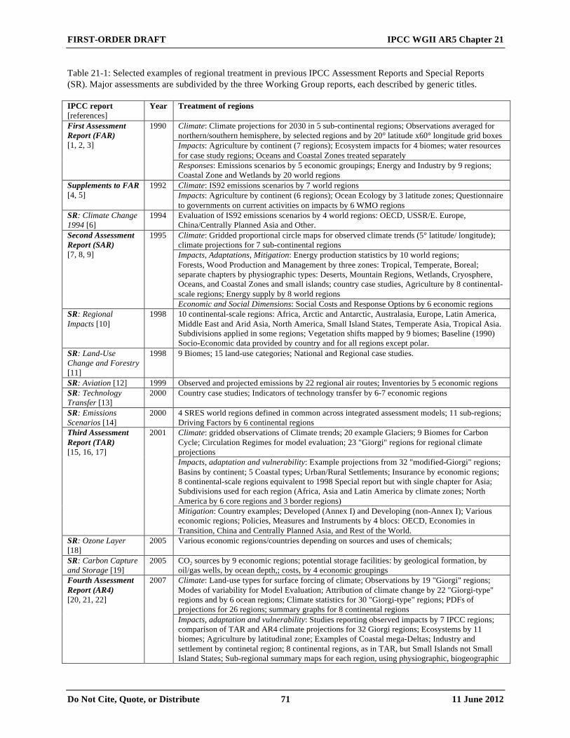
FIRST-ORDER DRAFT IPCC WGII AR5 Chapter 21
Do Not Cite, Quote, or Distribute 71 11 June 2012
Table 21-1: Selected examples of regional treatment in previous IPCC Assessment Reports and Special Reports (SR). Major assessments are subdivided by the three Working Group reports, each described by generic titles. IPCC report [references]
Year Treatment of regions
First Assessment Report (FAR) [1, 2, 3]
1990 Climate: Climate projections for 2030 in 5 sub-continental regions; Observations averaged for northern/southern hemisphere, by selected regions and by 20° latitude x60° longitude grid boxes Impacts: Agriculture by continent (7 regions); Ecosystem impacts for 4 biomes; water resources for case study regions; Oceans and Coastal Zones treated separately Responses: Emissions scenarios by 5 economic groupings; Energy and Industry by 9 regions; Coastal Zone and Wetlands by 20 world regions
Supplements to FAR [4, 5]
1992 Climate: IS92 emissions scenarios by 7 world regions Impacts: Agriculture by continent (6 regions); Ocean Ecology by 3 latitude zones; Questionnaire to governments on current activities on impacts by 6 WMO regions
SR: Climate Change 1994 [6]
1994 Evaluation of IS92 emissions scenarios by 4 world regions: OECD, USSR/E. Europe, China/Centrally Planned Asia and Other.
Second Assessment Report (SAR) [7, 8, 9]
1995 Climate: Gridded proportional circle maps for observed climate trends (5° latitude/ longitude); climate projections for 7 sub-continental regions Impacts, Adaptations, Mitigation: Energy production statistics by 10 world regions; Forests, Wood Production and Management by three zones: Tropical, Temperate, Boreal; separate chapters by physiographic types: Deserts, Mountain Regions, Wetlands, Cryosphere, Oceans, and Coastal Zones and small islands; country case studies, Agriculture by 8 continental-scale regions; Energy supply by 8 world regions Economic and Social Dimensions: Social Costs and Response Options by 6 economic regions
SR: Regional Impacts [10]
1998 10 continental-scale regions: Africa, Arctic and Antarctic, Australasia, Europe, Latin America, Middle East and Arid Asia, North America, Small Island States, Temperate Asia, Tropical Asia. Subdivisions applied in some regions; Vegetation shifts mapped by 9 biomes; Baseline (1990) Socio-Economic data provided by country and for all regions except polar.
SR: Land-Use Change and Forestry [11]
1998 9 Biomes; 15 land-use categories; National and Regional case studies.
SR: Aviation [12] 1999 Observed and projected emissions by 22 regional air routes; Inventories by 5 economic regions SR: Technology Transfer [13]
2000 Country case studies; Indicators of technology transfer by 6-7 economic regions
SR: Emissions Scenarios [14]
2000 4 SRES world regions defined in common across integrated assessment models; 11 sub-regions; Driving Factors by 6 continental regions
Third Assessment Report (TAR) [15, 16, 17]
2001 Climate: gridded observations of Climate trends; 20 example Glaciers; 9 Biomes for Carbon Cycle; Circulation Regimes for model evaluation; 23 "Giorgi" regions for regional climate projections Impacts, adaptation and vulnerability: Example projections from 32 "modified-Giorgi" regions; Basins by continent; 5 Coastal types; Urban/Rural Settlements; Insurance by economic regions; 8 continental-scale regions equivalent to 1998 Special report but with single chapter for Asia; Subdivisions used for each region (Africa, Asia and Latin America by climate zones; North America by 6 core regions and 3 border regions) Mitigation: Country examples; Developed (Annex I) and Developing (non-Annex I); Various economic regions; Policies, Measures and Instruments by 4 blocs: OECD, Economies in Transition, China and Centrally Planned Asia, and Rest of the World.
SR: Ozone Layer [18]
2005 Various economic regions/countries depending on sources and uses of chemicals;
SR: Carbon Capture and Storage [19]
2005 CO2 sources by 9 economic regions; potential storage facilities: by geological formation, by oil/gas wells, by ocean depth,; costs, by 4 economic groupings
Fourth Assessment Report (AR4) [20, 21, 22]
2007 Climate: Land-use types for surface forcing of climate; Observations by 19 "Giorgi" regions; Modes of variability for Model Evaluation; Attribution of climate change by 22 "Giorgi-type" regions and by 6 ocean regions; Climate statistics for 30 "Giorgi-type" regions; PDFs of projections for 26 regions; summary graphs for 8 continental regions Impacts, adaptation and vulnerability: Studies reporting observed impacts by 7 IPCC regions; comparison of TAR and AR4 climate projections for 32 Giorgi regions; Ecosystems by 11 biomes; Agriculture by latitudinal zone; Examples of Coastal mega-Deltas; Industry and settlement by continetal region; 8 continental regions, as in TAR, but Small Islands not Small Island States; Sub-regional summary maps for each region, using physiographic, biogeographic

FIRST-ORDER DRAFT IPCC WGII AR5 Chapter 21
Do Not Cite, Quote, or Distribute 72 11 June 2012
or geographic definitions; Example vulnerability maps at sub-national scale and globally by country. Mitigation: 17 global economic regions for GDP; Energy supply by continent, by economic regions, by 3 UNFCCC groupings; Trends in CO2 emissions (and projections) , waste and carbon balance by economic regions,
SR: Renewable Energy Sources and Climate Change Mitigation [23]
2011 Global maps showing potential resources for renewable energy: land suitability for bioenergy production, global irradiance for solar, geoethermal, hydropower, ocean waves/tidal range, wind); Various economic/continental regions: installed capacity (realised vs. potential), types of technologies, investment cost, cost effectiveness, various scenario-based projections; Country comparisons of deployment and uptake of technologies, share of energy market.
SR: Managing the Risks of Extreme Events and Disasters to Advance Climate Change Adaptation [24]
2012 Trends in observed (tables) and projected (maps and tables) climate extremes (Tmax, Tmin, heat waves, heavy precipitation and dryness) by 26 sub-continental regions covering most land areas of the globe; Attribution studies of return periods of extreme temperatures for 15 "Giorgi-type" regions; Gridded global maps of projected extremes of temperature, precipitation, windspeed, dry spells and soil moisture anomalies; Continental-scale estimates of projected changes in impacts of extremes (floods, cyclones, coastal inundation) as well as frequencies of observed climate extremes and their estimated costs); Distinctions drawn between local, country and international/global actors with respect to risk management and its financing.
1. IPCC (1990c), 2. IPCC (1990a); 3. IPCC (1990b); 4. IPCC (1992b); 5. IPCC (1992a); 6. IPCC (1994) 7. IPCC (1996c); 8. IPCC (1996b); 9. IPCC (1996a); 10. IPCC (1998b); 11. IPCC (1998a); 12. IPCC (1999); 13. IPCC (2000a), 14. IPCC (2000b); 15. IPCC (2001c); 16. IPCC (2001a); 17. IPCC (2001b); 18. IPCC/TEAP (2005); 19. IPCC (2005); 20. IPCC (2007c); 21. IPCC (2007a); 22. IPCC (2007b); 23. IPCC (2011); 24. IPCC (2012)

FIRST-ORDER DRAFT IPCC WGII AR5 Chapter 21
Do Not Cite, Quote, or Distribute 73 11 June 2012
Table S21-2: [Proposed that this be moved supplementary material] Countries and territories of the world, their regional treatment in this report and some other illustrative groupings of relevance for international climate change policy making. Sources (status in May 2012): AOSIS (2012), Arctic Council (2012), European Commission (2012), G77 (2012), OECD (2012), OHRLLS (2012), OPEC (2012), Secretariat of the Antarctic Treaty (2012), UNCLOS (2012), UNFCCC (1992, 1998, 2012). [If supplementary material, possibly to be used in conjunction with an interactive map and other statistical information, e.g. population, GDP, HDI?]
UN member state and other territories (+) Cha
pter
of
this
Rep
ort
UN
FCC
C
Ann
ex B
OEC
D
OEC
D O
DA
LLD
Cs
SID
S
Tran
sitio
n Ec
onom
ies
AO
SIS
G77
and
C
hina
OPE
C
Euro
pean
U
nion
Ant
arct
ic
Trea
ty
Arc
tic
Cou
ncil
UN
CO
LS
Afghanistan 24 3 1 1 1 2 Albania 23 4 4 1 1 Algeria 22 3 4 1 1 1 American Samoa (+) 29 2 2 Andorra 23 Angola 22 3 1 1 1 1 Anguilla (+) 29 4 2 Antigua and Barbuda 29 3 4 1 1 1 1 Argentina 27, 28 3 4 1 1 1 Armenia 23 4 3 1 1 1 Aruba (+) 29 2 Australia 25, 28 2 1 1 1 1 Austria 23 2 1 1 1 2 1 Azerbaijan 24 3 4 1 1 Bahamas 29 3 1 1 1 1 Bahrain 24 3 1 1 1 Bangladesh 24 3 1 1 1 Barbados 29 3 1 1 1 1 Belarus 23 3 4 1 2 1 Belgium 23 2 1 1 1 1 1 Belize 27 3 3 1 1 1 1 Benin 22 3 1 1 1 Bhutan 24 3 1 1 1 2 Bolivia 27 3 3 1 1 1 Bosnia and Herzegovina 23 3 4 1 1 1 Botswana 22 3 4 1 1 1 Brazil 27 3 3 4 1 1 1

FIRST-ORDER DRAFT IPCC WGII AR5 Chapter 21
Do Not Cite, Quote, or Distribute 74 11 June 2012
UN member state and other territories (+) Cha
pter
of
this
Rep
ort
UN
FCC
C
Ann
ex B
OEC
D
OEC
D O
DA
LLD
Cs
SID
S
Tran
sitio
n Ec
onom
ies
AO
SIS
G77
and
C
hina
OPE
C
Euro
pean
U
nion
Ant
arct
ic
Trea
ty
Arc
tic
Cou
ncil
UN
CO
LS
British Virgin Islands (+) 29 2 Brunei Darussalam 24 3 1 1 Bulgaria 23 1 1 1 1 1 Burkina Faso 22 3 1 1 1 1 Burundi 22 3 1 1 1 2 Cambodia 24 3 1 1 2 Cameroon 22 3 3 1 1 Canada 26, 28 2 1 1 2 1 1 Cape Verde 29 3 3 1 1 1 1 Central African Republic 22 3 1 1 1 2 Chad 22 3 1 1 1 1 Chile 27, 28 3 1 4 1 1 1 China 24 3 3 4 1 1 1 Colombia 27 3 4 1 2 2 Commonwealth of the Northern Mariana Islands (+) 29 2 Comoros 29 3 1 1 1 1 1 Congo 22 3 3 1 1 Cook Islands (+) 29 3 4 2 1 1 Costa Rica 27 3 4 1 1 Côte d'Ivoire 22 3 3 1 1 Croatia 23 1 1 1 2 1 Cuba 29 3 4 1 1 1 2 1 Cyprus 29 3 1 1 1 Czech Republic 23 1 1 1 1 2 1 Democratic People's Republic of Korea 24 3 2 1 2 2 Democratic Republic of the Congo 22 3 1 1 1 Denmark 23, 28 2 1 1 1 2 1 1 Djibouti 22 3 1 1 1 Dominica 27 3 4 1 1 1 1 Dominican Republic 27 3 4 1 1 1 Ecuador 27 3 4 1 1 1 Egypt 22 3 3 1 1

FIRST-ORDER DRAFT IPCC WGII AR5 Chapter 21
Do Not Cite, Quote, or Distribute 75 11 June 2012
UN member state and other territories (+) Cha
pter
of
this
Rep
ort
UN
FCC
C
Ann
ex B
OEC
D
OEC
D O
DA
LLD
Cs
SID
S
Tran
sitio
n Ec
onom
ies
AO
SIS
G77
and
C
hina
OPE
C
Euro
pean
U
nion
Ant
arct
ic
Trea
ty
Arc
tic
Cou
ncil
UN
CO
LS
El Salvador 27 3 3 1 2 Equatorial Guinea 22 3 1 1 1 Eritrea 22 3 1 1 Estonia 23 1 1 1 1 2 1 Ethiopia 22 3 1 1 1 2 European Union (+) 23 2 1 1 Fiji 29 3 3 1 1 1 1 Finland 23, 28 2 1 1 1 1 1 1 France 23 2 1 1 1 1 2 1 French Polynesia (+) 29 2 Gabon 22 3 4 1 1 Gambia 22 3 1 1 1 Georgia 24 3 3 1 1 Germany 23 2 1 1 1 1 2 1 Ghana 22 3 3 1 1 Greece 23 2 1 1 1 2 1 Grenada 29 3 4 1 1 1 1 Guam (+) 29 2 2 Guatemala 27 3 3 1 2 1 Guinea 22 3 1 1 1 Guinea-Bissau 22 3 1 1 1 1 1 Guyana 27 3 3 1 1 1 1 Haiti 27 3 1 1 1 1 1 Holy See (+) 23 Honduras 27 3 3 1 1 Hungary 23 1 1 1 1 2 1 Iceland 23, 28 2 1 1 2 1 1 India 24 3 3 3 1 1 1 Indonesia 24 3 3 3 1 1 Iran (Islamic Republic of) 24 3 4 1 1 2 Iraq 24 3 3 1 1 1 Ireland 23 2 1 1 1 1

FIRST-ORDER DRAFT IPCC WGII AR5 Chapter 21
Do Not Cite, Quote, or Distribute 76 11 June 2012
UN member state and other territories (+) Cha
pter
of
this
Rep
ort
UN
FCC
C
Ann
ex B
OEC
D
OEC
D O
DA
LLD
Cs
SID
S
Tran
sitio
n Ec
onom
ies
AO
SIS
G77
and
C
hina
OPE
C
Euro
pean
U
nion
Ant
arct
ic
Trea
ty
Arc
tic
Cou
ncil
UN
CO
LS
Israel 24 3 1 Italy 23 2 1 1 1 1 1 Jamaica 29 3 4 1 1 1 1 Japan 24 2 1 1 1 1 Jordan 24 3 4 1 1 Kazakhstan 24 4 4 1 1 Kenya 22 3 2 1 1 Kiribati 22 3 1 1 1 1 Kosovo (+) 23 3 Kuwait 24 3 1 1 1 Kyrgyzstan 24 3 2 1 1 Lao People's Democratic Republic 24 3 1 1 1 1 Latvia 23 1 1 1 1 Lebanon 24 3 4 1 1 Lesotho 22 3 1 1 1 1 Liberia 22 3 1 1 1 Libya 22 3 4 1 1 2 Liechtenstein 23 1 1 2 Lithuania 23 1 1 1 1 Luxembourg 23 2 1 1 1 1 Madagascar 22 3 1 1 1 Malawi 22 3 1 1 1 1 Malaysia 24 3 4 1 2 1 Maldives 29 3 4 1 1 1 1 Mali 22 3 1 1 1 1 Malta 29 3 1 1 1 Marshall Islands 29 3 3 1 1 1 1 Mauritania 22 3 1 1 1 Mauritius 29 3 4 1 1 1 1 Mexico 26 3 1 4 1 Micronesia (Federated States of) 29 3 3 1 1 1 1 Monaco 23 1 1 2 1

FIRST-ORDER DRAFT IPCC WGII AR5 Chapter 21
Do Not Cite, Quote, or Distribute 77 11 June 2012
UN member state and other territories (+) Cha
pter
of
this
Rep
ort
UN
FCC
C
Ann
ex B
OEC
D
OEC
D O
DA
LLD
Cs
SID
S
Tran
sitio
n Ec
onom
ies
AO
SIS
G77
and
C
hina
OPE
C
Euro
pean
U
nion
Ant
arct
ic
Trea
ty
Arc
tic
Cou
ncil
UN
CO
LS
Mongolia 24 3 3 1 1 1 Montenegro 23 3 4 1 2 1 Montserrat (+) 29 4 2 Morocco 22 3 3 1 1 Mozambique 22 3 1 1 1 Myanmar 24 3 1 1 1 Namibia 22 3 4 1 1 Nauru 29 3 4 1 1 1 1 Nepal 24 3 1 1 1 1 Netherlands 23 2 1 1 1 1 2 1 Netherlands Antilles (+) 29 2 2 New Caledonia (+) 29 2 New Zealand 25, 28 2 1 1 1 1 Nicaragua 27 3 3 1 1 Niger 22 3 1 1 1 2 Nigeria 22 3 3 1 1 1 Niue (+) 29 3 3 2 1 1 Norway 23, 28 2 1 1 1 1 1 Oman 24 3 1 1 Pakistan 24 3 3 1 2 1 Palau 29 3 4 1 1 1 Panama 27 3 4 1 1 Papua New Guinea 24 3 3 1 1 1 2 1 Paraguay 27 3 3 1 1 1 Peru 27 3 4 1 1 Philippines 24 3 3 1 1 Poland 23 1 1 1 1 1 2 1 Portugal 23 2 1 1 1 2 1 Puerto Rico (+) 29 2 Qatar 24 3 1 1 1 Republic of Korea 24 3 1 1 1 Republic of Moldova 23 4 3 1 1 1

FIRST-ORDER DRAFT IPCC WGII AR5 Chapter 21
Do Not Cite, Quote, or Distribute 78 11 June 2012
UN member state and other territories (+) Cha
pter
of
this
Rep
ort
UN
FCC
C
Ann
ex B
OEC
D
OEC
D O
DA
LLD
Cs
SID
S
Tran
sitio
n Ec
onom
ies
AO
SIS
G77
and
C
hina
OPE
C
Euro
pean
U
nion
Ant
arct
ic
Trea
ty
Arc
tic
Cou
ncil
UN
CO
LS
Romania 23 1 1 1 2 1 Russian Federation 23, 24, 28 1 1 2 1 1 1 1 Rwanda 22 3 1 1 1 2 Saint Kitts and Nevis 29 3 4 1 1 1 1 Saint Lucia 29 3 4 1 1 1 1 Saint Vincent and the Grenadines 29 3 4 1 1 1 1 Samoa 29 3 1 1 1 1 1 San Marino 23 3 Sao Tome and Principe 29 3 1 1 1 1 1 Saudi Arabia 24 3 1 1 1 Senegal 22 3 1 1 1 Serbia 23 3 4 1 2 1 Seychelles 29 3 4 1 1 1 1 Sierra Leone 22 3 1 1 1 Singapore 29 3 1 1 1 1 Slovakia 23 1 1 1 1 2 1 Slovenia 23 1 1 1 1 1 Solomon Islands 29 3 1 1 1 1 1 Somalia 22 3 1 1 1 South Africa 22 3 3 4 1 1 1 South Sudan 22 2 Spain 23 2 1 1 1 1 2 1 Sri Lanka 24 3 3 1 1 St Helena (+) 29 4 Sudan 22 3 1 1 1 Suriname 25 3 4 1 1 1 1 Swaziland 22 3 3 1 1 2 Sweden 23, 28 2 1 1 1 1 1 1 Switzerland 23 2 1 1 2 1 Syrian Arab Republic 22 3 3 1 Tajikistan 24 3 2 1 1 1 Thailand 24 3 4 1 1

FIRST-ORDER DRAFT IPCC WGII AR5 Chapter 21
Do Not Cite, Quote, or Distribute 79 11 June 2012
UN member state and other territories (+) Cha
pter
of
this
Rep
ort
UN
FCC
C
Ann
ex B
OEC
D
OEC
D O
DA
LLD
Cs
SID
S
Tran
sitio
n Ec
onom
ies
AO
SIS
G77
and
C
hina
OPE
C
Euro
pean
U
nion
Ant
arct
ic
Trea
ty
Arc
tic
Cou
ncil
UN
CO
LS
The former Yugoslav Republic of Macedonia 23 3 4 1 1 2 1 Timor-Leste 24 3 1 1 1 Togo 22 3 1 1 1 Tokelau (+) 29 3 Tonga 29 3 3 1 1 1 1 Trinidad and Tobago 29 3 1 1 1 1 Tunisia 22 3 4 1 1 Turkey 23 1 1 4 2 2 Turkmenistan 24 4 3 1 1 1 Tuvalu 29 3 1 1 1 1 U.S. Virgin Islands (+) 29 2 2 Uganda 22 3 1 1 1 1 Ukraine 23 1 1 3 1 1 1 United Arab Emirates 24 3 1 1 2 United Kingdom of Great Britain and Northern Ireland 23, 28 2 1 1 1 1 2 1 United Republic of Tanzania 22 3 1 1 1 United States of America 26, 28 2 1 1 1 1 Uruguay 27 3 4 1 1 1 Uzbekistan 24 4 3 1 1 Vanuatu 29 3 1 1 1 1 1 Venezuela (Bolivarian Republic of) 27 3 4 1 1 2 Viet Nam 24 3 3 1 1 Wallis and Futuna (+) 29 4 West Bank and Gaza Strip (+) 24 3 1 Yemen 24 3 1 1 1 Zambia 22 3 1 1 1 1 Zimbabwe 22 3 2 1 1 1
Key to country groupings and numerical codes. UNFCCC (United Nations Framework Convention on Climate Change) Parties – 1: Annex I, 2: Annex II, 3: Non-Annex I, 4: Non-Annex I Special Decision; Annex B Parties to the Kyoto Protocol – 1: Annex B; OECD (Organisation for Economic Co-operation and Development) – 1: Member, 2: Accession process, 3: Enhanced engagement; OECD ODA (Overseas Development Assistance) – 1: Least developed, 2: Other low income, 3: Lower middle income, 4: Upper middle income; LLCDs (Landlocked Developing Countries) – 1: Member; SIDS (Small Island Developing States) – 1: UN Member, 2: Non-UN/Associate; Transition Economies – 1: UN designated; AOSIS (Alliance of Small Island States) – 1: Member, 2: Observer; G77 (Group of 77) and China – 1: Member; OPEC (Organization of the Petroleum Exporting Countries) – 1: Member; European Union – 1: Member State, 2: Candidate; Antarctic Treaty Parties – 1: Consultative, 2: Non-Consultative; Arctic Council – 1: Member, 2: Permanent Observer; UNCOLS (United Nations Convention on the Law of the Sea) – 1: Ratified, 2: Signed but not Ratified.

FIRST-ORDER DRAFT IPCC WGII AR5 Chapter 21
Do Not Cite, Quote, or Distribute 80 11 June 2012
Table 21-3: [PLACEHOLDER] Comparative table that will summarise vulnerability findings in key systems according to the first half of WG2’s contribution in the different regions as laid out in the second half of WG2’s contribution. Urban Rural Food &
Water Coasts Ecosystems Industry and
Infrastructure Africa Europe Asia Australasia North America Central and South America
Polar Regions Small Islands Open Oceans Table 21-4: [PLACEHOLDER] Comparative table that will summarise impacts findings in key systems according to the first half of WG2’s contribution in the different regions as laid out in the second half of WG2’s contribution. Urban Rural Food &
Water Coasts Ecosystems Industry and
Infrastructure Africa Europe Asia Example of
what could be here: Rice growing areas in Mekong, Red River, Irrawaddy and Ganges-Brahmaputra Deltas (Chapter 5)
Australasia North America Central and South America
Polar Regions Small Islands Open Oceans

FIRST-ORDER DRAFT IPCC WGII AR5 Chapter 21
Do Not Cite, Quote, or Distribute 81 11 June 2012
Table 21-5: [PLACEHOLDER] Comparative table that will summarise adaptation issues in key systems according to the first half of WG2’s contribution in the different regions as laid out in the second half of WG2’s contribution. Urban Rural Food &
Water Coasts Ecosystems Industry and
Infrastructure Africa Europe Asia Australasia North America Central and South America
Polar Regions Small Islands Open Oceans Table 21-6: [PLACEHOLDER] Comparative table that will summarise sectoral issues in key systems according to the first half of WG2’s contribution in the different regions as laid out in the second half of WG2’s contribution. Urban Rural Food &
Water Coasts Ecosystems Industry and
Infrastructure Africa Europe Asia Australasia North America Central and South America
Polar Regions Small Islands Open Oceans

FIRST-ORDER DRAFT IPCC WGII AR5 Chapter 21
Do Not Cite, Quote, or Distribute 82 11 June 2012
Figure 21-1: [PLACEHOLDER] Maps showing the 26 regions (land areas only) used to summarise projected changes in climate in this chapter (upper panel – IPCC, 2012) and the regions defined for Chapters 22-29 in Part B (lower panel – IPCC, 2001). Note that information is also provided in this chapter on projected climate over the open oceans. [Maps to be redrawn and combined when climate regions and AR5 chapter regions clarified]
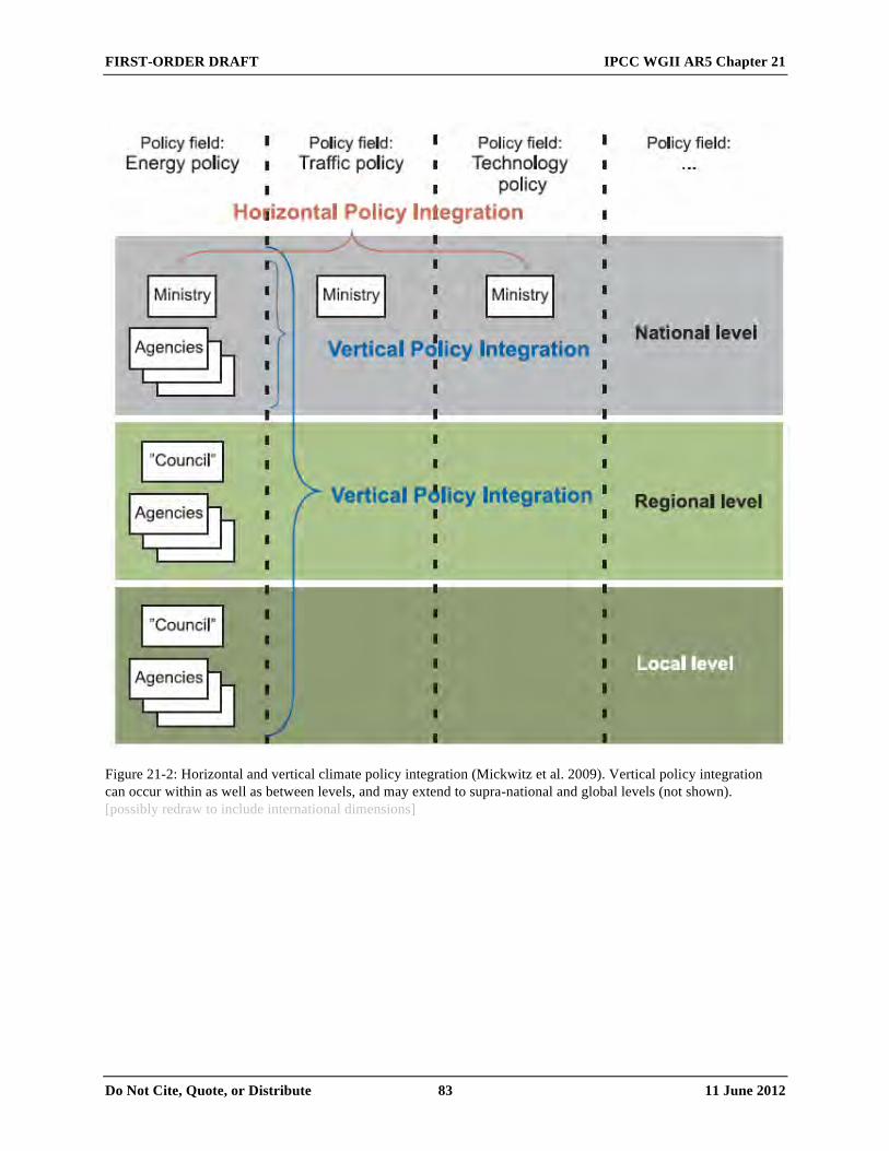
FIRST-ORDER DRAFT IPCC WGII AR5 Chapter 21
Do Not Cite, Quote, or Distribute 83 11 June 2012
Figure 21-2: Horizontal and vertical climate policy integration (Mickwitz et al. 2009). Vertical policy integration can occur within as well as between levels, and may extend to supra-national and global levels (not shown). [possibly redraw to include international dimensions]

FIRST-ORDER DRAFT IPCC WGII AR5 Chapter 21
Do Not Cite, Quote, or Distribute 84 11 June 2012
a) 2-year return period
b) 20-year return period
Figure 21-3: The range of percentage change in flood peaks for nine UK catchments at the a) 2-year and b) 20-year return period. Box-and-whisker plots are used to summarise results when using 10,000 UKCP09 Sampled Data (Murphy et al. 2009) change factors (red) and 100 sets of UKCP09 current and future Weather Generator time-series (cyan). Also plotted, are the results when using 11 sets of RCM-derived change factors (red crosses) and when using 11 sets of RCM current and future times-series (green rectangles). The box delineates the 25th-75th percentile range and the whiskers the 10th-90th percentile range, with the median (50th percentile) shown by the line dividing the box. Additional markers outside the whiskers indicate the minima and maxima, if within the plotted range of -50 to +100. The points derived from the RCM results are joined for the corresponding members of the RCM ensemble (grey lines), and the medians for these methods are shown by black horizontal bars.

FIRST-ORDER DRAFT IPCC WGII AR5 Chapter 21
Do Not Cite, Quote, or Distribute 85 11 June 2012
Figure 21-4: Time series of seasonally averaged climate indices representing (a) the tropical September to January Pacific Walker Circulation (PWC), (b) the December to March North Atlantic Oscillation (NAO), and (c) the December to March Pacific North America (PNA) pattern. Indices are calculated from various sources: 20CRv2 (pink); statistical reconstructions using Bronnimann et al. (2009) for the PWC, Griesser et al. (2010) for the PNA, and HadSLP2 (Allan and Ansell, 2006) for the NAO (all cyan); NCEP–NCAR reanalyses (NNR; dark blue); ERA-40 (green); ERA-Interim (orange); and SOCOL ensemble mean (dark grey). The light grey shading indicates the minimum and maximum range of the SOCOL ensemble. All indices are computed with respect to the overlapping 1989–1999 period. Indices are defined as in Brönnimann etal. (2009).

FIRST-ORDER DRAFT IPCC WGII AR5 Chapter 21
Do Not Cite, Quote, or Distribute 86 11 June 2012
Figure 21-5: Observed 1990-2007 annual precipitation climatology from GPCC (Rudolf et al., 2011), top left, and, in the remaining panels, related systematic errors in 9 individual regional climate model simulations driven by the ERA-Interim reanalyses (Dee et al., 2011) and in the multi-model ensemble mean.

FIRST-ORDER DRAFT IPCC WGII AR5 Chapter 21
Do Not Cite, Quote, or Distribute 87 11 June 2012
Figure 21-6: Variations in past and future regional climate over Africa. Precipitation plots cover land territory only, while temperature plots cover both land and exclusive economic zone territory. Black lines show annual average values from observational datasets and coloured bands show the 10-90th percentile range of annual average values from 32 simulations from 12 climate models from the WCRP CMIP3 and CMIP5 projects (Meehl et al. 2007, Taylor et al. 2012). The pink band is from simulations driven with observed changes in all known external drivers over the 1901-2005 period. The blue band is from simulations driven with observed changes in natural external drivers only. The green band is from simulations running over 2006-2050 driven under either the SRES A1B or the RCP4.5 emissions scenario. Observed values are plotted as anomalies from their 1901-2005 averages. Model values are plotted as anomalies from their 1901-2005 averages in the simulation with all know drivers.

FIRST-ORDER DRAFT IPCC WGII AR5 Chapter 21
Do Not Cite, Quote, or Distribute 88 11 June 2012
Figure 21-7: Evolution of the 5%, 17%, 33%, 50%, 66%, 83% and 95% percentiles of the distribution functions for annual surface air temperature changes (upper panel) and annual precipitation (lower panel) for the Giorgi-Francisco (2000) regions and the globe with the A1B forcing scenario. Twenty year means relative to the 1961-1990 baseline are plotted in decadal steps using a common y-axis scale. The 5%, 50% and 95% percentile values for the period 2080-2099 are displayed for each region. (From Harris et al. 2012)

FIRST-ORDER DRAFT IPCC WGII AR5 Chapter 21
Do Not Cite, Quote, or Distribute 89 11 June 2012
Figure 21-8: The relative aggregate climate change between the 1975-2005 period and the 2010-2039, 2040-2069 and 2070-2099 periods of RCP8.5. The aggregate climate change is calculated using the Standard Euclidean Distance (SED) across the 28-dimensional climate space formed by 7 climate variables in each of 4 seasons. The absolute values of change in each variable are normalized to the maximum global absolute value prior to calculating the SED. The SED values are then normalized to the maximum global SED value. Only land grid points north of 60˚S are used in the normalizations (From Diffenbaugh and Giorgi 2012).

FIRST-ORDER DRAFT IPCC WGII AR5 Chapter 21
Do Not Cite, Quote, or Distribute 90 11 June 2012
Figure 21-9: Monthly values of the zonally averaged changes in mean surface air temperature (top left panel), temperature interannual variability (as measured by the standard deviation, top right panel), mean precipitation (bottom left panel), precipitation interannual variability (as measured by the coefficient of variation) over Europe; CMIP3 ensemble, A1B scenario, 2071-2100 minus 1961-1990. Units are degrees C for temperature and % of 1961-1990 values for mean precipitation (the coefficient of variation is unitless). The zonal average is taken over the region between 10°W and 25°E. The dashed lines illustrate the European Climate Change Oscillation (ECO). From Giorgi and Coppola (2007).

FIRST-ORDER DRAFT IPCC WGII AR5 Chapter 21
Do Not Cite, Quote, or Distribute 91 11 June 2012
Figure 21-10: Linear changes of annual precipitation during the 2001-2050 period from 10 individual RCM experiments and the MME mean under the A1B emission scenario. The top middle panels also account for projected land cover changes (see text for further explanation). Note that the REMO trends in both panels arise from a three-member ensemble whereas all other RCMs are represented by one single simulation. Trends statistically significant at the 5% level are marked by black dots. (From Paeth et al. 2011)

FIRST-ORDER DRAFT IPCC WGII AR5 Chapter 21
Do Not Cite, Quote, or Distribute 92 11 June 2012
Figure 21-11: Change in summer (JJA) average temperature (2041-2070 minus 1971-2000) from (top left) the NCAR CCSM3, (top right) the MM5 regional climate model driven by the CCSM3; (bottom left) the WRF model, driven by CCSM3, and (bottom right) the Canadian CRCM, driven by CCSM3. Temperature is in °C. Data from the NARCCAP program. (From Mearns et al., 2009, 2011)

FIRST-ORDER DRAFT IPCC WGII AR5 Chapter 21
Do Not Cite, Quote, or Distribute 93 11 June 2012
Figure 21-12: Mean (top panels) and standard deviation (bottom panels) in future-minus-present MDA8 summer ozone concentrations across (left-hand panels) all 7 experiments (5 regional and 2 global) and, for comparison purposes (right-hand panels) not including the WSU experiment (which simulated July only conditions). (From Weaver et al. 2009)

FIRST-ORDER DRAFT IPCC WGII AR5 Chapter 21
Do Not Cite, Quote, or Distribute 94 11 June 2012
Figure 21-13: Difference in average summer daily ozone mean (left panel) and peak (right panel) concentration over Europe due to climate change, A2 scenario. (From Meleux et al. 2007)

FIRST-ORDER DRAFT IPCC WGII AR5 Chapter 21
Do Not Cite, Quote, or Distribute 95 11 June 2012
Figure 21-14: Growth rates from 1990-2008 of international trade, its embodied CO2 emissions and net emissions transfers from Annex B and non-Annex B countries compared to other global macrovariables, all indexed to 1990 (Peters et al., 2011). (Notes: Screen captured image - Carter)

FIRST-ORDER DRAFT IPCC WGII AR5 Chapter 21
Do Not Cite, Quote, or Distribute 96 11 June 2012
(a) (b) Figure 21-15: (To be reworked) Projected change (a) in accessibility of maritime and land-based transportation by mid-century (2045-2059 relative to 2000-2014) using the Arctic Transport Accessibility Model and CCSM3 climate and sea ice estimates assuming an SRES A1B scenario. Green areas denote new maritime access to Type A vessels (light icebreaker); white areas remain inaccessible. Red delimits areas of lost winter road potential for ground vehicles exceeding 2 metric tonnes (Stephenson et al., 2011). Route (b) of the Northwest Passage and Northern Sea Route (right), which is part of the Northeast Passage (Government Office for Science, 2011). [Could also add the Arctic Bridge and North Pole routes]
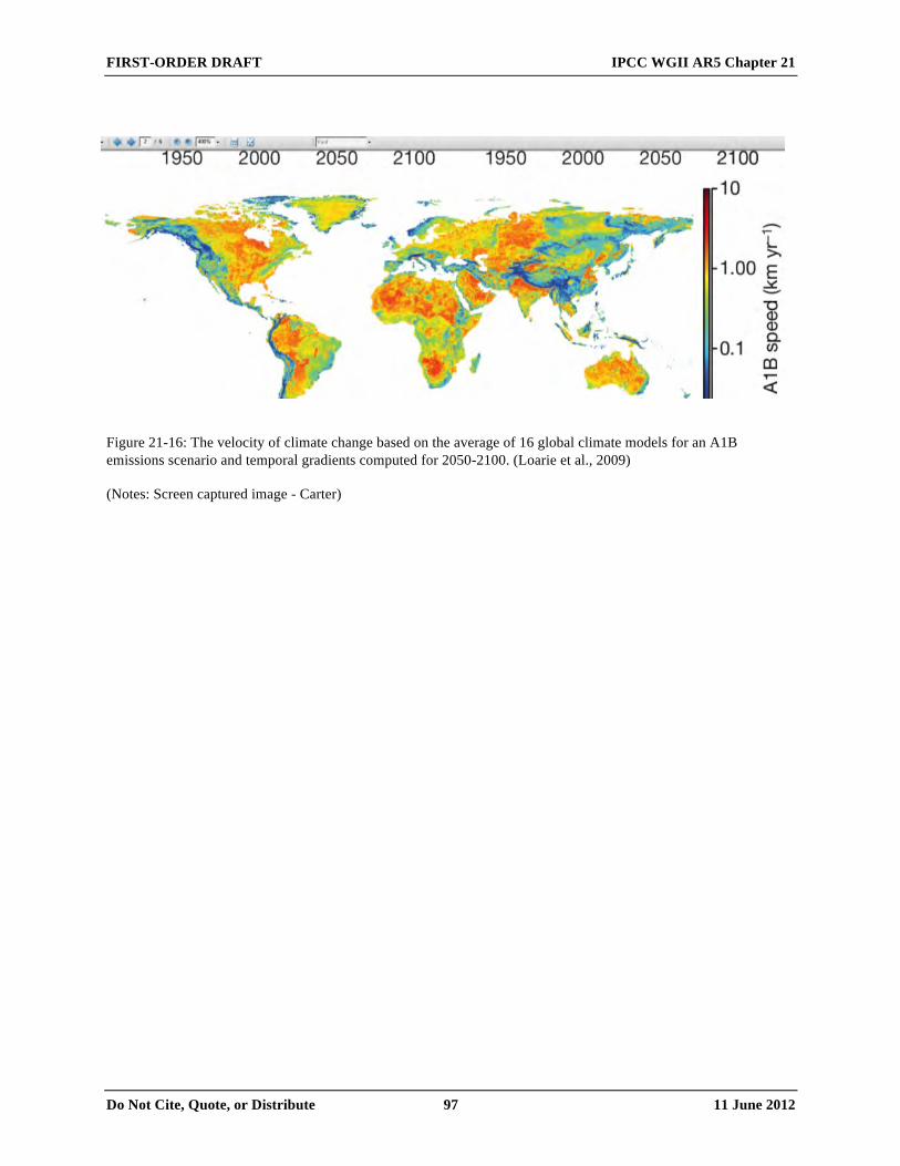
FIRST-ORDER DRAFT IPCC WGII AR5 Chapter 21
Do Not Cite, Quote, or Distribute 97 11 June 2012
Figure 21-16: The velocity of climate change based on the average of 16 global climate models for an A1B emissions scenario and temporal gradients computed for 2050-2100. (Loarie et al., 2009) (Notes: Screen captured image - Carter)