
First Draft SP 800-90B · 2018-09-27 · The attached DRAFT document (AUGUST 2012 draft of: SP...
80
The attached DRAFT document (AUGUST 2012 draft of: SP 800-90B) (is provided here for historical purposes) has been superseded by the following updated draft publication: Publication Number: DRAFT SP 800-90B (second draft) Title: Recommendation for the Entropy Sources Used for Random Bit Generation Publication Date: January 27, 2016 January 2016 Draft Publication with full announcement details: http://csrc.nist.gov/publications/PubsDrafts.html#800-90B
Transcript of First Draft SP 800-90B · 2018-09-27 · The attached DRAFT document (AUGUST 2012 draft of: SP...

The attached DRAFT document (AUGUST 2012 draft of: SP 800-90B) (is provided here for
historical purposes) has been superseded by the following updated draft publication:
Publication Number: DRAFT SP 800-90B (second draft)
Title: Recommendation for the Entropy Sources Used for
Random Bit Generation
Publication Date: January 27, 2016
January 2016 Draft Publication with full announcement details:
http://csrc.nist.gov/publications/PubsDrafts.html#800-90B

Announcement of 2nd draft SP 800-90B Released:
January 27, 2016
Draft SP 800-90 Series: Random Bit Generators
Recommendation for the Entropy Sources Used for Random Bit Generation
NIST announces the second draft of Special Publication (SP) 800-90B, Recommendation for the
Entropy Sources Used for Random Bit Generation. This Recommendation specifies the design
principles and requirements for the entropy sources used by Random Bit Generators, and the
tests for the validation of entropy sources. These entropy sources are intended to be combined
with Deterministic Random Bit Generator mechanisms that are specified in SP 800-90A to
construct Random Bit Generators, as specified in SP 800-90C. NIST is planning to host a
workshop on Random Number Generation to discuss the SP 800-90 series, specifically, SP 800-
90B and SP 800-90C. More information about the workshop is available at:
http://www.nist.gov/itl/csd/ct/rbg_workshop2016.cfm.
The specific areas where comments are solicited on SP 800-90B are:
Post-processing functions (Section 3.2.2): We provided a list of approved post-processing
functions. Is the selection of the functions appropriate?
Entropy assessment (Section 3.1.5): While estimating the entropy for entropy sources
using a conditioning component, the values of n and q are multiplied by the constant
0.85. Is the selection of this constant reasonable?
Multiple noise sources: The Recommendation only allows using multiple noise sources if
the noise sources are independent. Should the use of dependent noise sources also be
allowed, and if so, how can we calculate an entropy assessment in this case?
Health Tests: What actions should be taken when health tests raise an alarm? The
minimum allowed value of a type I error for health testing is selected as 2-50. Is this
selection reasonable?
NIST requests comments on the revised (second) Draft SP 800-90B by 5:00PM EST on May 9,
2016. Please submit comments on Draft SP 800-90B using the comments template form (Excel
Spreadsheet – see link below) to [email protected] with “Comments on Draft SP 800-
90B” in the subject line.
NIST DRAFT Special Publication 800-90B
Recommendation for the Entropy Sources Used for Random Bit
Generation
Elaine Barker
John Kelsey
Computer Security Division
Information Technology Laboratory
C O M P U T E R S E C U R I T Y
August 2012
U.S. Department of Commerce John Bryson, Secretary
National Institute of Standards and Technology
Patrick D. Gallagher, Under Secretary for Standards and Technology and Director

NIST SP 800-90B (DRAFT) August 2012
ii
Abstract
This Recommendation specifies the design principles and requirements for the entropy
sources used by Random Bit Generators, and the tests for the validation of entropy sources.
These entropy sources are intended to be combined with Deterministic Random Bit
Generator mechanisms that are specified in [SP 800-90A] to construct Random Bit
Generators, as specified in [SP 800-90C].
KEY WORDS: deterministic random bit generator (DRBG); entropy; hash function;
random number generator; noise source; entropy source; conditioning component

NIST SP 800-90B (DRAFT) August 2012
iii
Acknowledgements
The National Institute of Standards and Technology (NIST) gratefully acknowledges and
appreciates contributions by Mike Boyle and Mary Baish from the National Security
Agency for assistance in the development of this Recommendation. NIST also thanks the
many contributions by the public and private sectors.

NIST SP 800-90B (DRAFT) August 2012
iv
Table of Contents
1.0 Scope .............................................................................................................. 8
2.0 Terms and Definitions ................................................................................... 9
3.0 Symbols and Abbreviated Terms ............................................................... 16
4.0 General Discussion ..................................................................................... 18
4.1 Entropy Estimation and Validation ............................................................................ 18
4.2 Entropy .......................................................................................................................... 19
4.3 The Entropy Source Model.......................................................................................... 19
4.3.1 Noise Source ................................................................................................... 20
4.3.2 Conditioning Component ............................................................................... 20
4.3.3 Health Tests ..................................................................................................... 21
5.0 Conceptual Interfaces ................................................................................. 21
5.1.1 GetEntropy: An Interface to the Entropy Source ......................................... 21
5.1.2 GetNoise: An Interface to the Noise Source ................................................ 22
5.1.3 Health Test: An Interface to the Entropy Source ......................................... 22
6.0 Entropy Source Development Requirements ............................................ 23
6.1 General Requirements for Design and Validation .................................................... 23
6.2 Full Entropy Source Requirements ............................................................................ 24
6.3 Noise Source Requirements ....................................................................................... 25
6.4 Conditioning Component Requirements ................................................................... 25
6.4.1 Non-Approved Conditioning Components ................................................... 26
6.4.2 Approved Cryptographic Conditioning Components ................................. 26
6.4.2.1 Approved Keyed Conditioning Functions .................................... 26
6.4.2.2 Approved Unkeyed Conditioning Functions ............................... 28
6.4.2.3 Recommendations for Improved Security ................................... 29
6.5 Health Test Requirements ........................................................................................... 29
6.5.1 Health Tests on the Noise Source ................................................................. 29
6.5.1.1 General Requirements ................................................................... 29
6.5.1.2 Continuous Testing ........................................................................ 30
6.5.1.3 Start-up and On-Demand Testing ................................................. 37
6.5.2 Health Tests on the Conditioning Component ............................................ 38

NIST SP 800-90B (DRAFT) August 2012
v
7.0 Validation Data and Documentation Requirements.................................. 38
7.1 General Validation Requirements .............................................................................. 38
7.2 Dealing with the Data Requirement for Noise Sources with Large Output Spaces ........................................................................................................................... 41
8.0 Entropy Source Testing Strategy ............................................................... 42
8.1 General Noise Source Entropy Testing Strategy ...................................................... 42
8.2 Entropy Source Testing Strategy for Conditioned Output ...................................... 45
8.3 Entropy Source Testing Strategy for Full Entropy Sources .................................... 46
8.4 Entropy Source Testing Strategy for the Health Test Component ......................... 47
9.0 Tests for Determining Entropy Provided by Entropy Sources ................ 48
9.1 Determining if the Data is IID ...................................................................................... 48
9.1.1 General Discussion ......................................................................................... 48
9.1.2 Shuffling Tests on Independence and Stability ........................................... 48
9.1.2.1 Compression Score ........................................................................ 50
9.1.2.2 Over/Under Runs Scores (Two Scores) ....................................... 51
9.1.2.3 Excursion Score ............................................................................. 52
9.1.2.4 Directional Runs Scores (Three scores) ...................................... 52
9.1.2.5 Covariance Score ........................................................................... 54
9.1.2.6 Collision Score (Three scores) ...................................................... 55
9.1.3 Specific Statistical Tests ................................................................................ 56
9.1.3.1 Chi-Square Test .............................................................................. 56
9.1.3.2 Other Statistical Tests .................................................................... 60
9.2 Estimating the Min-Entropy of IID Sources ............................................................... 61
9.3 Estimating the Min-Entropy of non-IID Sources ....................................................... 61
9.3.1 General Discussion ......................................................................................... 61
9.3.2 Testing Summary ............................................................................................ 62
9.3.3 The Collision Test ........................................................................................... 62
9.3.3.1 Test Overview.................................................................................. 62
9.3.3.2 Implementation Summary .............................................................. 63
9.3.3.3 Collision Test Details ..................................................................... 63
9.3.4 The Partial Collection Test ............................................................................ 65
9.3.4.1 Test Overview.................................................................................. 65
NIST SP 800-90B (DRAFT) August 2012
vi
9.3.4.2 Implementation Summary .............................................................. 65
9.3.4.3 Partial Collection Test Details ....................................................... 66
9.3.5 The Markov Test .............................................................................................. 67
9.3.5.1 Test Overview.................................................................................. 67
9.3.5.2 Implementation Summary .............................................................. 68
9.3.5.3 Markov Test Details ........................................................................ 68
9.3.6 The Compression Test ................................................................................... 69
9.3.6.1 Test Overview.................................................................................. 69
9.3.6.2 Implementation Summary .............................................................. 69
9.3.6.3 Compression Test Details .............................................................. 69
9.3.7 The Frequency Test ........................................................................................ 71
9.3.7.1 Test Overview.................................................................................. 71
9.3.7.2 Implementation Summary .............................................................. 72
9.3.7.3 Frequency Test Details .................................................................. 72
9.4 Sanity Checks Against Entropy Estimates ................................................................ 73
9.4.1 Compression Sanity Check ........................................................................... 73
9.4.2 Collision Sanity Check ................................................................................... 73
9.4.2.1 General Description ........................................................................ 73
9.4.2.2 Testing Noise Sources With an Entropy Estimate per Sample .. 74
10.0 Health Test Validation: Testing for Equivalent Functionality .................. 75
10.1 Demonstrating Equivalent Functionality to the Repetition Count Test ................. 76
10.2 Demonstrating Equivalent Functionality to the Adaptive Proportion Test ............ 76
Annex A: References ........................................................................................... 78

NIST SP 800-90B (DRAFT) August 2012
vii
Authority
This publication has been developed by the National Institute of Standards and Technology
(NIST) in furtherance of its statutory responsibilities under the Federal Information
Security Management Act (FISMA) of 2002, Public Law 107-347.
NIST is responsible for developing standards and guidelines, including minimum
requirements, for providing adequate information security for all agency operations and
assets, but such standards and guidelines shall not apply to national security systems.
This recommendation has been prepared for use by Federal agencies. It may be used by
nongovernmental organizations on a voluntary basis and is not subject to copyright.
(Attribution would be appreciated by NIST.)
Nothing in this Recommendation should be taken to contradict standards and guidelines
made mandatory and binding on federal agencies by the Secretary of Commerce under
statutory authority. Nor should this Recommendation be interpreted as altering or
superseding the existing authorities of the Secretary of Commerce, Director of the OMB, or
any other federal official.
Conformance testing for implementations of this Recommendation will be conducted
within the framework of the Cryptographic Algorithm Validation Program (CAVP) and the
Cryptographic Module Validation Program (CMVP). The requirements of this
Recommendation are indicated by the word “shall.” Some of these requirements may be
out-of-scope for CAVP or CMVP validation testing, and thus are the responsibility of
entities using, implementing, installing or configuring applications that incorporate this
Recommendation.

NIST SP 800-90B (DRAFT) August 2012
8
Recommendation for the Entropy Sources Used for Random Bit Generation
1.0 Scope
Cryptography and security applications make extensive use of random numbers and
random bits. However, the generation of random bits is problematic in many practical
applications of cryptography. The purpose of NIST Special Publication (SP) 800-90B is to
specify the design and testing requirements for entropy sources that can be validated as
approved entropy sources by NIST’s CAVP and CMVP. SPs 800-90A and 800-90C
address the construction of approved Deterministic Random Bit Generator (DRBG)
mechanisms and approved Random Bit Generators (RBGs) that utilize the entropy sources
and DRBG mechanisms, respectively.
An entropy source that conforms to this Recommendation generates random bits, primarily
for use in cryptographic applications. While there has been extensive research on the
subject of generating pseudorandom bits using a DRBG and an unknown seed value,
creating such an unknown value has not been as well documented. The only way for this
seed value to provide real security is for it to contain a sufficient amount of randomness,
i.e., from a non-deterministic process referred to as an entropy source. SP 800-90B
describes the properties that an entropy source must have to make it suitable for use by
cryptographic random bit generators, as well as the tests used to validate the quality of the
entropy source.
The development of entropy sources that provide unpredictable output is difficult, and
providing guidance for their design and validation testing is even more so. The testing
approach defined in this Recommendation assumes that the developer understands the
behavior of the entropy source and has made a good-faith effort to produce a consistent
source of entropy. It is expected that, over time, improvements to the guidance and testing
will be made, based on experience in using and validating against this Recommendation.
SP 800-90B is based on American National Standard (ANS) X9.82, Part 2, Random
Number Generation, Part 2: Entropy Sources [X9.82-2].
NIST SP 800-90B (DRAFT) August 2012
9
2.0 Terms and Definitions
Algorithm
A clearly specified mathematical process for computation; a set of rules that, if followed,
will give a prescribed result.
Approved
FIPS-approved or NIST-recommended.
Assessment (of Entropy)
An evaluation of the amount of entropy provided by a (digitized) noise source and/or the
entropy source that employs it.
Biased
A random process (or the output produced by such a process) is said to be biased with
respect to an assumed discrete set of potential outcomes (i.e., possible output values) if
some of those outcomes have a greater probability of occurring than do others. Contrast
with unbiased.
Binary Data (from a Noise Source)
Digitized output from a noise source that consists of a single bit; that is, each sampled
output value is represented as either 0 or 1.
Bitstring
A bitstring is a finite sequence (string) of 0’s and 1’s. The left-most bit is the most
significant bit in the bitstring. The right-most bit is the least significant bit of the bitstring.
Collision
An instance of duplicate sample values occurring in a dataset.
Conditioning (of Noise Source Output)
A method of post-processing the output of a (digitized) noise source to reduce bias and/or
ensure that the entropy rate of the conditioned output is no less than some specified
amount. Full entropy output is not necessarily provided.
Conditioning Component
An optional component of an entropy source used to post-process the output of its noise
source with the intent of reducing bias and/or increasing the entropy rate of the resulting
output to ensure that it meets some specific threshold. (See Conditioning, above.)

NIST SP 800-90B (DRAFT) August 2012
10
Continuous Test
A health test performed within an entropy source on the output of its noise source, in order
to gain some level of assurance that the noise source is working correctly, prior to
producing each output from the entropy source.
Consuming Application (for an RBG)
An application that uses the output from an approved random bit generator.
Cryptographic Hash Function
A function that maps bitstrings of arbitrary length (up to some maximum) to bitstrings of
fixed length (determined by the particular function) and is expected to have, at least, the
following three properties:
1. Collision resistance: It is computationally infeasible to find two distinct input
bitstrings that map to the same output bitstring;
2. Preimage resistance: Given a bitstring of the same length as those output by the
function (but not previously observed as the output corresponding to a known
input), it is computationally infeasible to find an input bitstring that maps to the
given bitstring;
3. Second-preimage resistance: Given one input bitstring (and the corresponding
bitstring output by the function), it is computationally infeasible to find a
second (distinct) input bitstring that maps to the same output bitstring.
Dataset
A sequence of sample values. (See Sample.)
Deterministic Random Bit Generator (DRBG)
An RBG that employs a DRBG mechanism and a source of entropy input. A DRBG
produces a pseudorandom sequence of bits from an initial secret value called a seed (and,
perhaps additional input). A DRBG is often called a Pseudorandom Bit (or Number)
Generator.
DRBG mechanism
The portion of an RBG that includes the functions necessary to instantiate and
uninstantiate a DRBG, generate pseudorandom bits, (optionally) reseed the DRBG and test
the health of the DRBG mechanism. Approved DRBG mechanisms are specified in [SP
800-90A].
Entropy
The (Shannon) entropy of a discrete random variable X is the expected amount of
information that will be provided by an observation of X. (See information content.) In this
Standard, the information content is measured in bits; when the expected information
content of an observation of X is m bits, we say that the random variable X has m bits of
entropy.

NIST SP 800-90B (DRAFT) August 2012
11
Entropy is defined relative to one's knowledge of (the probability distribution on) X prior
to an observation, and reflects the uncertainty associated with predicting its value – the
larger the entropy, the greater the uncertainty in predicting the value of an observation.
In the case of a discrete random variable, the entropy of X is determined by computing the
sum of p(x) log2(p(x)), where x varies over all possible values for an observation of X and
p(x) is the (a priori) probability that an observation will have value x.
If there are N distinct possibilities for an observation of X, then the maximum possible
value for the entropy of X is log2(N) bits, which is attained when X has the uniform
probability distribution (i.e., when the N possible observations are equally likely to occur).
See also min-entropy.
Entropy Rate
The rate at which a digitized noise source (or entropy source) provides entropy; it is
computed as the assessed amount of entropy provided by a bitstring output from the
source, divided by the total number of bits in the bitstring (yielding assessed bits of
entropy per output bit). This will be a value between zero (no entropy) and one (full
entropy).
Entropy Source
A source of random bitstrings. There is no assumption that the bitstrings are output in
accordance with a uniform distribution. The entropy source includes a noise source (e.g.,
thermal noise or hard drive seek times), health tests, and an optional conditioning
component.
False Alarm
An erroneous indication that a component has malfunctioned, despite the fact that the
component was behaving correctly. See also False Positive.
False Positive
An erroneous acceptance of the hypothesis that a statistically significant event has been
observed. This is also referred to as a Type 1 error. When ‘health-testing’ the components
of a device, it often refers to a declaration that a component has malfunctioned – based on
some statistical test(s) – despite the fact that the component was actually working
correctly. See False Alarm.
Full Entropy
Ideally, to say that a bitstring provides “full entropy” would imply that it was selected
uniformly at random from the set of all bitstrings of its length – in which case, each bit in
the string would be uniformly distributed (i.e., equally likely to be 0 or 1) and statistically
independent of the other bits in the string. However, for the purposes of this
Recommendation, an n-bit string is said to provide full entropy if it is obtained through a
process that is estimated to provide at least (1) n bits of entropy, where 0 2-64
. Such
strings are an acceptable approximation to the ideal.

NIST SP 800-90B (DRAFT) August 2012
12
Full Entropy Source
An entropy source that is designed to output bitstrings providing full entropy output. See
Full Entropy, above.
Hash Function
See Cryptographic Hash Function. Hash algorithm and cryptographic hash function are
used interchangeably in this Recommendation.
Health Test
A test that is run to check that a mechanism continues to behave as expected.
Health Testing
Testing within an implementation prior to or during normal operation to determine that the
implementation continues to perform as expected and as validated.
Independent
Two discrete random variables X and Y are (statistically) independent if the probability that
an observation of X will have a certain value does not change, given knowledge of the
value of an observation of Y (and vice versa). When this is the case, the probability that the
observed values of X and Y will be x and y, respectively, is equal to the probability that the
observed value of X will be x (determined without regard for the value of y) multiplied by
the probability that the observed value of Y will be y (determined without regard for the
value of x).
Independent and Identically Distributed (IID)
A sequence of random variables for which each element of the sequence has the same
probability distribution as the other values and all values are mutually independent.
Known-Answer Test
A test that uses a fixed input/output pair (where the output is the correct output from the
component for that input), which is used to determine correct implementation and/or
continued correct operation.
Markov Model
A model for a probability distribution whereby the probability that the ith
element of a
sequence has a given value depends only on that value and the value of the previous k
elements of the sequence. The model is called a kth
order Markov model.
Min-entropy
The min-entropy (in bits) of a discrete random variable X is the largest value m having the
property that each observation of X provides at least m bits of information (i.e., the min-
entropy of X is the greatest lower bound for the information content of potential
observations of X). The min-entropy of X is a lower bound on its entropy. The precise
formulation for the min-entropy, m, for a given finite probability distribution, p1, …, pM, is
m = log2( max(p1,…, pM) ). Min-entropy is often used as a worst-case measure of the

NIST SP 800-90B (DRAFT) August 2012
13
uncertainty associated with observations of X: If X has min-entropy m, then the probability
of observing any particular value is no greater than 2-m
. (See also Entropy.)
Noise Source
The component of an entropy source that contains the non-deterministic, entropy-
producing activity.
Non-Deterministic Random Bit Generator (NRBG)
An RBG employing an entropy source, which (when working properly) produces outputs
that have full entropy (see Full Entropy). Also called a True Random Bit (or Number)
Generator.
On-demand Test
A health test that is available to be run whenever a user or a relying component requests it.
Output Space
The set of all possible bitstrings that may be obtained as samples from a digitized noise
source.
P-value
The probability (under the null hypothesis of randomness) that the chosen test statistic will
assume values that are equal to or more extreme than the observed test statistic value when
considering the null hypothesis. The p-value is frequently called the “tail probability.”
Probability Distribution
The probability distribution of a random variable X is a function F that assigns to the
interval [a, b] the probability that X lies between a and b (inclusive).
Probability Model
A mathematical representation of a random phenomenon.
Pseudorandom
A deterministic process (or data produced by such a process) whose observed outcomes
(e.g., output values) are effectively indistinguishable from those of a random process, as
long as the internal states and internal actions of the process are hidden from observation.
For cryptographic purposes, “effectively indistinguishable” means “not within the
computational limits established by the intended security strength.”
Random
A non-deterministic process (or data produced by such a process) whose possible
outcomes (e.g., output values) are observed in accordance with some probability
distribution. The term is sometimes (mis)used to imply that the probability distribution is
uniform, but no such blanket assumption is made in this Recommendation.

NIST SP 800-90B (DRAFT) August 2012
14
Random Bit Generator (RBG)
A device or algorithm that is capable of producing a random sequence of (what are
effectively indistinguishable from) statistically independent and unbiased bits. An RBG is
classified as either a DRBG or an NRBG.
Sample (from a Digitized Noise Source)
An observation of the natural output unit from a digitized (but otherwise unprocessed)
noise source. Common examples of output values obtained by sampling are single bits,
single bytes, etc. (The term “sample” is often extended to denote a sequence of such
observations; this Recommendation will refrain from that practice.)
Security Boundary
A conceptual boundary that is used to assess the amount of entropy provided by the values
output from an entropy source. The entropy assessment is performed under the assumption
that any observer (including any adversary) is outside of that boundary.
Seed
Noun: A bitstring that is used as input to (initialize) an algorithm. In this
Recommendation, the algorithm using a seed is usually a DRBG. The entropy provided by
the seed must be sufficient to support the intended security strength of the DRBG.
Verb: To acquire a bitstring using a process that provides sufficient entropy for the desired
security strength and subsequently supply that bitstring to (initialize) an algorithm (e.g., a
DRBG).
Sequence
An ordered list of quantities.
Shall
Used to indicate a requirement of this Recommendation.
Should
Used to indicate a highly desirable feature that is not necessarily required by this
Recommendation.
Source of entropy input (SEI)
A component of an RBG that outputs bitstrings that can be used as entropy input by a
DRBG mechanism. See [SP 800-90C].
Stable Distribution
A random variable is stable if it has the property that linear combinations of two
independent copies of the variable have the same distribution; i.e., let X1 and X2 be
independent copies of a random variable X. Then X is said to be stable if for any constants
a>0 and b>0 the random variable aX1 + bX2 has the same distribution as cX + d for some
constants c>0 and d.

NIST SP 800-90B (DRAFT) August 2012
15
Startup Testing (of an Entropy Source)
A suite of health tests that are performed every time the entropy source is initialized or
powered up. These tests are carried out before any output is released from the entropy
source.
String
See Sequence.
Testing Laboratory
An entity that has been accredited to perform cryptographic security testing on an entropy
source, as specified in this Recommendation.
Unbiased
A random process (or the output produced by such a process) is said to be unbiased with
respect to an assumed discrete set of potential outcomes (e.g., possible output values) if
each of those outcomes has the same probability of occurring. (Contrast with biased.) A
pseudorandom process is said to be unbiased if it is effectively indistinguishable from an
unbiased random process (with respect to the same assumed discrete set of potential
outcomes). For cryptographic purposes, “effectively indistinguishable” means “not within
the computational limits established by the intended security strength.”

NIST SP 800-90B (DRAFT) August 2012
16
3.0 Symbols and Abbreviated Terms
The following symbols are used in this document.
Symbol Meaning
H The min-entropy of the samples from a (digitized) noise source or
of the output from an entropy source; the min-entropy assessment
for a noise source or entropy source.
hamming_weight(si,…,si+n) The number of ones in the sequence si, si+1, …, si+n.
max(a, b) The maximum of the two values, a and b; e.g. if a>b, max(a, b) = a.
min(a, b) The minimum of the two values, a and b; e.g. if a<b, min(a, b) = a.
N The number of samples in a dataset, i.e., the length of the dataset in
samples.
n The number of bits that an entropy source can obtain as a single
(conditioned) output from its (digitized) noise source.
p(xi) or prob(xi) The probability for an observation or occurrence of xi.
pmax The probability of the most common sample from a noise source.
si A sample in a dataset.
S A dataset.
xi A possible output from the (digitized) noise source.
[a,b] The interval of numbers between a and b, including a and b.
x A function that returns the smallest integer greater than or equal to
x; also known as the ceiling function.
x A function that returns the largest integer less than or equal to x;
also known as the floor function.
Round(x) A function that returns the integer that is closest to x. If x lies half-
way between two integers, the larger integer is returned.
Sqrt(x) or √𝑥 A function that returns a number y whose square is x. For example,
Sqrt(16) = 4.
The following abbreviations are used in this document.
Abbreviations Meaning
ANS American National Standard
CAVP Cryptographic Algorithm Validation Program

NIST SP 800-90B (DRAFT) August 2012
17
CMAC Cipher-based Message Authentication Code, as specified in
SP800-38B
CMVP Cryptographic Module Validation Program
DRBG Deterministic Random Bit Generator
FIPS Federal Information Processing Standard
HMAC Keyed-Hash Message Authentication Code, specified in [FIPS 198]
IID Independent and Identically Distributed
NIST National Institute of Standards and Technology
NRBG Non-deterministic Random Bit Generator
NVLAP National Voluntary Laboratory Accreditation Program
RBG Random Bit Generator
SP NIST Special Publication
NIST SP 800-90B (DRAFT) August 2012
18
4.0 General Discussion
Three things are required to build a cryptographic RBG. First, a source of random bits is
needed (the entropy source). Second, an algorithm (typically, a DRBG) is needed for
accumulating and providing these numbers to the consuming application. Finally, there
needs to be a way to combine the first two components appropriately for the cryptographic
application.
SP 800-90B describes how to design and implement the entropy source. SP 800-90A
describes deterministic algorithms that take an entropy input and use it to produce
pseudorandom values. SP 800-90C provides the “glue” for putting the entropy source
together with the algorithm to implement an RBG.
Specifying an entropy source is a complicated matter. This is partly due to confusion in the
meaning of entropy, and partly due to the fact that, while other parts of an RBG design are
strictly algorithmic, entropy sources depend on physical processes that may vary from one
instance of a source to another. This section discusses, in detail, both the entropy source
model and the meaning of entropy.
4.1 Entropy Estimation and Validation
The developer should make every effort to design an entropy source that can be shown to
serve as a consistent source of entropy, producing bitstrings that can provide entropy at a
rate that meets (or exceeds) a specified value.
In order to design an entropy source that provides an adequate amount of entropy per
output bitstring, the developer must be able to accurately estimate the amount of entropy
that can be provided by sampling its (digitized) noise source. The developer must also
understand the behavior of the other components included in the entropy source, since the
interactions between the various components will affect any assessment of the entropy that
can be provided by an implementation of the design.
For example, if it is known that the (digitized) output from the noise source is biased,
appropriate conditioning functions can be included in the design to reduce that bias to a
tolerable level before any bits are output from the entropy source. Likewise, if the
developer estimates that the noise source employed provides entropy at a rate of (at least)
½ bit of entropy per bit of (digitized) sample, that assessment will likely be reflected in the
number of samples that are combined by a conditioning component to produce bitstrings
with an entropy rate that meets the design requirements for the entropy source.
This Recommendation provides requirements and guidance that will allow for an entropy
source to be validated and for an assessment of the entropy to be performed that will show
the entropy source produces bitstrings that can provide entropy at a specified rate.
Validation provides additional assurance that adequate entropy is provided by the source
and may be necessary to satisfy some legal restrictions, policies, and/or directives of
various organizations.

NIST SP 800-90B (DRAFT) August 2012
19
4.2 Entropy
The central mathematical concept underlying this Recommendation is entropy. Entropy is
defined relative to one's knowledge of X prior to an observation, and reflects the
uncertainty associated with predicting its value – the larger the entropy, the greater the
uncertainty in predicting the value of an observation. There are many possible choices for
an entropy measure; this Recommendation uses a very conservative measure known as
min-entropy.
Min-entropy is often used as a worst-case measure of the uncertainty associated with
observations of X: If X has min-entropy m, then the probability of observing any particular
value is no greater than 2-m
. Let xi be a digitized sample from the noise source that is
represented in one or more bits, let x1, x2, ..., xM be the outputs from the noise source, and
let p(xi) be the probability that xi is produced at any given sampling time. The min-entropy
of the outputs is:
log2 (max p(xi)).
This represents the best-case work for an adversary who is trying to guess an output from
the noise source. For an in-depth discussion of entropy and the use of min-entropy in
assessing an entropy source, see ANS X9.82, Part 1 [X9.82-1].
4.3 The Entropy Source Model
This section considers the entropy source in detail. Figure 1 illustrates the model that this
Recommendation uses to describe an entropy source, including the components that an
entropy source developer shall implement. These components are described in the
following sections. Additional detail on each component can be found in ANS X9.82, Part
2 [X9.82-2].

NIST SP 800-90B (DRAFT) August 2012
20
4.3.1 Noise Source
The noise source is the root of security for the entropy source and for the RBG as a whole.
This is the component that contains the non-deterministic, entropy-providing activity that
is ultimately responsible for the uncertainty associated with the bitstrings output by the
entropy source. If this component fails, no other mechanism in the RBG can compensate
for the lack of entropy.
Fundamentally, the noise source provides random bits in the form of digital samples
obtained from a non-deterministic process. If the non-deterministic process being sampled
produces something other than binary data, the sampling process includes digitization.
This Recommendation assumes that the sample values obtained from a noise source
consist of fixed-length bitstrings, which determine the output space of the component.
4.3.2 Conditioning Component
The optional conditioning component is responsible for reducing bias and/or increasing the
entropy rate of the resulting output bits (if necessary to obtain a target value). There are
various methods for achieving this. In choosing an approach to implement, the developer
may either choose to implement an approved cryptographic algorithm or a non-approved
algorithm (see Section 6.4). The use of either of these approaches is permitted by this
Noise Source
Digitization
(Optional)
Conditioning
AssessmentHealth
Testing
OUTPUT
ENTROPY
SOURCE
Noise Source
Digitization
(Optional)
Conditioning
AssessmentHealth
Testing
OUTPUT
ENTROPY
SOURCE
Figure 1: Entropy Source Model
Noise Source
Digitization
(Optional) Conditioning
Health Testing
OUTPUT
ENTROPY
SOURCE
Noise Source
Digitization
(Optional)
Conditioning
AssessmentHealth
Testing
OUTPUT
ENTROPY
SOURCE
Figure 1: Entropy Source Model Figure 1: Entropy Source Model

NIST SP 800-90B (DRAFT) August 2012
21
Recommendation. The developer should consider the conditioning method and how
variations in the behavior of the noise source may affect the entropy rate of the output.
This will assist in determining the best approach to use when implementing a conditioning
component.
4.3.3 Health Tests
Health tests are an integral part of the entropy source design; the health test component
ensures that the noise source and the entropy source as a whole continue to operate as
expected. The health tests can be separated into three categories; startup tests (on all
components), continuous tests (mostly on the noise source), and on-demand tests (tests that
are more thorough and time-consuming than the continuous tests).
Behavior tests, a type of health test, are performed on the parts of an implementation for
which an exact response cannot be predicted (i.e., the noise source, for which the behavior
is non-deterministic); normally, the acceptable responses are expected within a specified
range of all possible responses. Behavior tests may be performed at specified times or may
be performed continuously.
When testing the entropy source, the end goal is to obtain assurance that failures of the
entropy source are caught quickly and with a high probability. Another aspect of health
testing strategy is determining likely failure modes for the entropy source and, in
particular, for the noise source. Comprehensive health tests will include tests that can
detect these failure conditions.
5.0 Conceptual Interfaces
5.1.1 GetEntropy: An Interface to the Entropy Source
This section describes a conceptual interface to the entropy source that is compatible with
the RBG interfaces in [SP 800-90C]. The interface described here can be considered to be
a command interface into the outer entropy source box in Figure 1. This interface is meant
to indicate the types of requests for services that an entropy source may support.
A GetEntropy call returns a bitstring and an assessment of the entropy it provides.
GetEntropy( ):
Output:
entropy_bitstring The string that provides the requested entropy.
assessed_entropy An integer that indicates the assessed number of bits of entropy
provided by entropy_bitstring.
status A boolean value that is TRUE if the request has been satisfied,
and is FALSE otherwise.
It should be noted that the interface defined here includes a return value indicating the
amount of entropy provided by the returned bitstring. In practice, assessed_entropy does
NIST SP 800-90B (DRAFT) August 2012
22
not need to be returned as output if the amount of entropy provided by entropy_bitstring
would already be known to the relying application (e.g., in implementations for which the
amount of entropy provided is a predefined constant).
5.1.2 GetNoise: An Interface to the Noise Source
The conceptual interface defined here can be considered to be a command interface into
the noise source component of an entropy source. This is used to obtain raw, digitized, but
otherwise unprocessed, outputs from the noise source for use in validation testing or for
external health tests. While it is not required to be in this form, it is expected that an
interface exist such that the data can be obtained without harm to the entropy source. This
interface is meant to provide test data to credit a noise source with an entropy estimate
during validation or for health testing, and as such, does not contribute to the generation of
entropy source output. It is feasible that such an interface is available only in “test mode”
and that it is disabled when the source is operational.
This interface is not intended to constrain real-world implementations, but to provide a
consistent notation to describe data collection from noise sources. Thus, the interface may
indicate, for example, that a noise source generates bits in response to a request from the
entropy source, when, in practice, the noise source may be passing random bits to the
entropy source as the bits are generated; i.e., it ‘pushes’ data to the entropy source as it
becomes available.
A GetNoise call returns raw, digitized, but otherwise unprocessed samples from the noise
source.
GetNoise(number_of_samples_requested)
Input:
number_of_samples_requested An integer value that indicates the requested
number of samples to be returned from the noise
source.
Output:
noise_source_data The sequence of samples from the noise source,
with length number_of_samples_requested.
status A boolean value that is TRUE if the request has
been satisfied, and is FALSE otherwise.
5.1.3 Health Test: An Interface to the Entropy Source
A HealthTest call is a request to the entropy source to conduct a test of its health. The
HealthTest interface allows for various testing methods since this Recommendation does
not require any particular on-demand health testing (see Section 6.5.1.3). Note that it may
not be necessary to include a separate HealthTest interface if the execution of the tests can
be initiated in another manner that is acceptable to [FIPS 140] validation.

NIST SP 800-90B (DRAFT) August 2012
23
HealthTest(type_of_test_requested)
Input:
type_of_test_requested A bitstring that indicates the type or suite of tests to be
performed (this may vary from one entropy source to
another).
Output:
pass-fail flag A boolean value that is TRUE if the entropy source
passed the requested test, and is FALSE otherwise.
6.0 Entropy Source Development Requirements
Included in the following sections are requirements for the entropy source as a whole, as
well as for each component individually. The intent of these requirements is to assist the
developer in designing/implementing an entropy source that can provide outputs with a
consistent amount of entropy and to provide the required documentation for entropy source
validation. The requirements below are intended to justify why the entropy source can be
relied upon.
6.1 General Requirements for Design and Validation
The functional requirements for the entropy source as a whole are as follows:
1. The developer shall document the design of the entropy source as a whole,
including the interaction of the components specified in Section 4.3. This
documentation shall justify why the entropy source can be relied upon to produce
bits with entropy.
2. The entropy source shall have a well-defined (conceptual) security boundary,
which shall be the same as or be contained within a [FIPS 140] cryptographic
module boundary. This security boundary shall be documented; the documentation
shall include:
A description of the content of the security boundary; note that the security
boundary may extend beyond the entropy source itself (e.g. the entropy
source may be contained within a larger boundary that also contains a
DRBG); also note that the security boundary may be logical, rather than
physical.
A description of how the security boundary ensures that an adversary
outside the boundary cannot reduce the entropy below the assessed entropy,
either through observation or manipulation.

NIST SP 800-90B (DRAFT) August 2012
24
Any assumptions concerning support functions (such as a power supply that
cannot be monitored or manipulated) upon which the security boundary
depends.
4. The developer shall document the range of operating conditions under which the
entropy source may be expected to continue to generate acceptable random data;
the documentation shall clearly describe the measures that have been taken in
system design to ensure the entropy source continues to operate correctly under
those conditions.
5. The entropy source shall be capable of being validated for conformance to [FIPS
140], and include appropriate interfaces to obtain test data, as described in Section
5.0.
6. Documentation shall be provided that describes the behavior of the noise source
and why it is believed that the entropy rate does not fluctuate during normal
operation.
7. Upon notification that the health tests have detected a malfunction, the entropy
source shall cease outputting data and should notify the consuming application
(e.g., the RBG) of the error condition.
An optional, recommended feature of the entropy source is as follows:
8. The entropy source may contain multiple noise sources to improve resiliency with
respect to degradation or misbehavior. When this feature is implemented, the
requirements specified in Section 6.3 shall apply to each noise source.
6.2 Full Entropy Source Requirements
Some of the RBG constructions in [SP 800-90C] depend on a Full Entropy Source, e.g. an
entropy source that closely approximates one in which each output bit is uniformly
distributed and independent of all other output bits. Additional requirements are levied on
sources that claim to provide full entropy output:
1. Bitstrings output from the entropy source shall provide at least (1)n bits of
entropy, where n is the length of each output string and 0 2-64
.
2. Noise source output, if conditioned, shall be conditioned with an approved
cryptographic conditioning function for full entropy to be provided by the entropy
source. At least twice the block size of the underlying cryptographic primitive
shall be provided as input to the conditioning function to produce full entropy
output.

NIST SP 800-90B (DRAFT) August 2012
25
6.3 Noise Source Requirements
The functional requirements for the noise source are as follows:
1. Although the noise source is not required to produce unbiased and independent
outputs, it shall exhibit probabilistic behavior; i.e., the output shall not be
definable by any known algorithmic rule.
2. The developer shall document the operation of the noise source; this
documentation shall include a description of how the noise source works and
rationale about why the noise provides acceptable entropy output, and should
reference relevant, existing research and literature.
3. The noise source shall be amenable to testing to ensure proper operation. In
particular, it shall be possible to collect data from the noise source for health
testing and during the validation process in order to allow an independent
determination of the entropy rate, and the appropriateness of the health tests on the
noise source. Acquiring outputs from the noise source shall not alter the behavior
of the noise source or affect the subsequent output in any way.
4. Failure or severe degradation of the noise source shall be detectable. Methods used
to detect such conditions shall be documented.
5. The noise source documentation shall describe the conditions, if any, under which
the noise source is known to malfunction or become inconsistent, including a
description of the range of environments in which the noise source can operate
correctly. Continuous tests or other mechanisms in the entropy source shall protect
against producing output during such malfunctions.
6. The noise source shall be protected from adversarial knowledge or influence to the
greatest extent possible. The methods used for this shall be documented, including
a description of the (conceptual) security boundary’s role in protecting the noise
source from adversarial observation or influence.
6.4 Conditioning Component Requirements
The functional requirements for the optional conditioning component are as follows:
1. The entropy source developer shall document whether or not the entropy source
performs conditioning. If conditioning depends on choices made external to the
entropy source (i.e. if it is a selectable option), this feature shall be documented.
2. If the entropy source performs conditioning, the method shall be described and
shall include an argument for how the chosen method meets its objectives with
respect to reducing the bias in the data obtained from the noise source and/or
producing output that meets (or exceeds) a specified entropy rate.
NIST SP 800-90B (DRAFT) August 2012
26
3. The entropy source conditioning component outputs shall be capable of being
subjected to health and validation testing.
4. The entropy source developer shall state and justify estimates of the bias and
entropy rate that is expected of the bitstrings output by the conditioning component.
If the entropy source is meant to produce full entropy output, the output bitstrings
shall satisfy the requirements in Section 6.2.
5. Documentation describing how variations in the behavior of the noise source will
affect the bias and entropy rate of the conditioning component’s output shall be
provided.
6.4.1 Non-Approved Conditioning Components
As discussed previously, there are various methods for designing a conditioning
component for an entropy source. One such method involves using a non-approved
conditioning function to condition the noise source outputs. If a non-approved
conditioning component is chosen in design of the entropy source, then this conditioning
component shall undergo extensive testing to determine the entropy provided by the
conditioned outputs (see Section 8.2). The entropy rate provided shall be no greater than
the entropy rate provided by the input to the conditioning component; full entropy shall
not be provided by non-approved conditioning components.
6.4.2 Approved Cryptographic Conditioning Components
Using an approved cryptographic function (i.e., algorithm) to condition the noise source
outputs is beneficial because the approved functions can uniformly distribute the input
entropy throughout the output of the conditioning component and as such can be used to
provide full entropy output. In general, the entropy estimate for the conditioning function
output will be no greater than the output length of the conditioning component.
This Recommendation approves both keyed and unkeyed functions for the conditioning
component, as discussed in Sections 6.4.2.1 and 6.4.2.2, respectively. These approved
conditioning functions produce the following results:
1. When an input string with m bits of assessed entropy is provided to an approved
conditioning function with an n-bit output, the resulting assessed entropy is
uniformly distributed across the entire n-bit output. Note that if 𝑚 ≥ 𝑛, full
entropy output is not necessarily provided; see item 2.
2. When an input string with 2n bits (or more) of assessed entropy is provided to an
approved conditioning function with an n-bit output, the resulting n-bit output is
considered to have full entropy.
6.4.2.1 Approved Keyed Conditioning Functions
Three keyed functions are approved for the conditioning component:
1. HMAC, as specified in [FIPS 198], with any approved hash function specified in
[FIPS 180],

NIST SP 800-90B (DRAFT) August 2012
27
2. CMAC, as specified in [SP 800-38B], with any approved block cipher algorithm
(see [FIPS 197] and [SP 800-67]), and
3. CBC-MAC, as specified in Section 6.4.2.1.2, with any approved block cipher
algorithm. CBC-MAC shall not be used for other purposes.
6.4.2.1.1 General Constructions for Approved Keyed Conditioning Functions
This general construction is to be used for the approved keyed conditioning functions listed
in Section 6.4.2.1. The following notation is used in the construction:
F(K, X) The notation used to represent the approved keyed conditioning function,
with key K and input string X.
n The number of bits output by F; for CMAC and CBC-MAC, n is the length
(in bits) of the output block of the block cipher algorithm; for HMAC, n is
the length (in bits) of the hash function output block.
S An input string with assessed entropy m.
A Additional input; any bit string, including the null string (e.g., a timestamp,
sequence number, or previous output value).
K Any key, e.g., a constant across all implementations, or a value initialized
once per entropy source, or initialized upon start-up.
Y The n-bit output of the conditioning function.
Process:
1. Y = F(K, S||A).
2. Output Y as the conditioned output.
If the input string S was assessed at 2n bits of min-entropy or more (i.e., 𝑚 ≥ 2𝑛), then Y
may be considered to have n bits of full entropy output. If S was assessed at m bits of min-
entropy and 2𝑛 > 𝑚 ≥ 𝑛, then Y shall be assessed at 𝑚
2 bits of min-entropy. If S was
assessed at m bits of min-entropy and 𝑚 < 𝑛 then Y shall be assessed at m bits of min-
entropy.
6.4.2.1.2 CBC-MAC Conditioning Function
For an approved conditioning function, CBC-MAC is defined as follows. This
construction shall not be used for any other purpose. The following notation is used for
the construction:
E(K,X) The notation used to represent the encryption of input string X using key K.
n The length (in bits) of the output block of the cipher algorithm.
S An input string; the length of S shall be an integer multiple of the output
length n of the block cipher algorithm and shall always be the same length
(i.e., variable length strings shall not be used as input).
w The number of n-bit blocks in S; an integer.

NIST SP 800-90B (DRAFT) August 2012
28
K The key to be used.
V The n-bit CBC-MAC output.
Process:
1. Let 𝑠0, 𝑠1, … 𝑠𝑤−1 be the sequence of blocks formed by dividing S into n-bit blocks;
i.e., each 𝑠𝑖 consists of n bits.
2. V = 0.
3. For i = 0 to w-1
V = E(K, V 𝑠𝑖).
4. Output V as the CBC-MAC output.
6.4.2.2 Approved Unkeyed Conditioning Functions
Three unkeyed functions are approved as conditioning functions:
1. Any approved hash function specified in [FIPS 180],
2. hash_df, as specified in [SP 800-90A], using any approved hash function
specified in [FIPS 180], and
3. bc_df, as specified in [SP800-90A], using any approved block cipher algorithm
(see [FIPS 197] and [SP 800-67]).
The following notation is used for the construction of the unkeyed conditioning function:
F(X) The notation used to represent the approved unkeyed conditioning function
listed above, applied to input string X.
S An input string assessed at m bits of entropy.
A Additional input; any bit string, including the null string (e.g. a timestamp,
sequence number or previous output value).
n The number of bits output by F; for bc_df, n is the length (in bits) of the
output block of the block cipher algorithm; otherwise, n is the length (in
bits) of the hash function output block.
Y The n-bit conditioned output.
Process:
1. Y = F(S||A).
2. Output Y as the conditioned output.
If the input string S was assessed at 2n bits of min-entropy or more (i.e., 𝑚 ≥ 2𝑛), then Y
may be considered to have n bits of full entropy output. If S was assessed at m bits of min-
entropy and 2𝑛 > 𝑚 ≥ 𝑛, then Y shall be assessed at 𝑚
2 bits of min-entropy. If S was

NIST SP 800-90B (DRAFT) August 2012
29
assessed at m bits of min-entropy and 𝑚 < 𝑛 then Y shall be assessed at m bits of min-
entropy.
6.4.2.3 Recommendations for Improved Security
The developer is permitted to select keys and additional input arbitrarily. However, the
following recommendations may improve security:
1. In the keyed functions in Section 6.4.2.1, the key K should be generated randomly
each time a device starts up (e.g., K can be obtained by using entropy bits from the
noise source with at least n bits of assessed entropy, where n is the output length of
the conditioning function to be used, and processing the entropy bits using the
conditioning function with an arbitrary key; the result can be used as K).
2. The optional additional input A should include some function of the previous
output from the conditioning function in order to smooth out variations in the
entropy source behavior.
6.5 Health Test Requirements
The objective of these tests is to detect deviations from the intended behavior of the
entropy source in general (and the noise source in particular) during operation. The
following are general requirements for entropy source health tests:
1. Testing shall be performed at startup and continuously thereafter to ensure that all
components of the entropy source continue to work correctly.
2. All entropy source health tests and their rationale shall be documented. The
documentation shall include a description of the health tests, the rate and
conditions under which each health test is performed (e.g., at startup, continuously,
or on-demand), the expected results for each health test, and rationale indicating
why each test is believed to be appropriate for detecting one or more failures in the
entropy source.
6.5.1 Health Tests on the Noise Source
6.5.1.1 General Requirements
The health testing of a noise source is likely to be very technology-specific. Since, in the
vast majority of cases, the noise source will not produce unbiased, independent binary
data, traditional statistical procedures (e.g., monobit, chi-square, and runs tests) that test
the hypothesis of unbiased, independent bits almost always fail, and thus are not useful for
monitoring the noise source. In general, tests on the noise source have to be tailored
carefully, taking into account the expected statistical behavior of the correctly operating
noise source.
Health testing of noise sources will typically be designed to detect failures of the noise
source based on the expected output during a failure, or to detect a deviation from the

NIST SP 800-90B (DRAFT) August 2012
30
expected output during the correct operation of the noise source. The following are
requirements for noise source health tests.
1. At a minimum, continuous testing as defined in Section 6.5.1.2 shall be
implemented. In addition, the developer shall document any known noise source
failure modes. Continuous tests should also be devised and implemented to detect
those failures.
2. Testing shall be performed on the digitized samples obtained from the noise
source.
3. The noise source shall be tested for variability in the output sample values. (A
sequence of outputs lacking in variability could, for example, consist of a single
repeated value.)
4. Noise source bits generated during start-up that have successfully passed the start-
up health tests may be used to produce entropy source output (after (optional)
conditioning).
5. When health testing detects a failure in the noise source, the entropy source shall
be notified.
Optional features for noise source health tests are:
6. Appropriate health tests tailored to the noise source should place special emphasis
on the detection of misbehavior near the boundary between the nominal operating
environment and abnormal conditions. This requires a thorough understanding of
the operation of the noise source.
6.5.1.2 Continuous Testing
The purpose of continuous testing is to allow the entropy source to detect many kinds of
disastrous failures in its underlying noise source. These tests are run continuously on all
digitized samples obtained from the noise source, and so must have a very low probability
of yielding a false positive. In many systems, a reasonable false positive rate will make it
extremely unlikely that a properly-functioning device will indicate a malfunction, even in a
very long service life. In the case where an error is identified, the noise source shall notify
the entropy source of the malfunction.
Note that the tests defined operate over a stream of values. These sample values may be
output as they are generated (i.e., processed by the conditioning component, as appropriate,
and used by the entropy source to produce output); there is no need to inhibit output from
the noise source or entropy source while running the test. It is important to understand that
this may result in poor entropy source outputs for a time since the error is only signaled
once significant evidence has been accumulated and these values may have already been
output by the source. As a result it is important that the false positive rate be set to an

NIST SP 800-90B (DRAFT) August 2012
31
acceptable level. Below, all calculations assume that a false positive rate of approximately
once per billion samples generated by the noise source is acceptable; however, the
formulas given can easily be adapted for even lower false positive probabilities, if
necessary.
Health tests are required for all entropy sources. The continuous tests discussed in this
Section are focused on noise source behavior and on detecting failures as the noise source
runs. The continuous tests shall:
Include the two tests below: the Repetition Count Test and the Adaptive Proportion
Test; or
Include other tests that detect the same failure conditions reliably, according to the
criteria given below in Section 10.0.
6.5.1.2.1 Repetition Count Test
The Repetition Count Test is an updated version of the "stuck bit" test—its goal is to
quickly detect a catastrophic failure that causes the noise source to become "stuck" on a
single output value for a long time. Given the assessed min-entropy, H, of the noise
source, it is easy to compute the probability that a sequence of N consecutive samples will
yield identical sample values. For example, a noise source with one bit of min-entropy per
sample has no more than a 1/2 probability of repeating some sample value twice in a row,
no more than 1/4 of repeating some sample value three times in a row, and in general, no
more than (1/2)N-1
probability of repeating some sample value N times in a row. More
generally, if a dataset of N consecutive sample values is obtained from a noise source with
H bits of min-entropy per sample, there is no greater than (2-H
)(N-1)
of obtaining a sequence
of N identical sample values.
This test's cutoff values can be applied to any entropy estimate, H, including very small
and very large estimates. However, it is important to note that this test is not very
powerful – it is able to detect only catastrophic failures of an entropy source. For example,
a noise source evaluated at eight bits of min-entropy per sample has a cutoff value of five
repetitions to ensure a false-positive rate of approximately once per four billion samples
generated. If that noise source somehow failed to the point that it was providing only four
bits of min-entropy per sample, it would still be expected to take about sixty-five thousand
samples before the Repetition Count Test would notice the problem.
As the noise source generates outputs, the entropy source keeps track of two variables and
a constant, C:
1. A = the most recently seen sample value.
2. B = the number of consecutive times that the value A has been seen.
3. C = the cutoff value at which the Repetition Count Test fails.
Therefore, running the Repetition Count Test requires enough memory to store A, B, and
C. The value of C does not need to be computed each time the test is run since C is
computed at design time as follows.

NIST SP 800-90B (DRAFT) August 2012
32
If W > 0 is the acceptable false-positive probability associated with an alarm
triggered by C repeated sample values, then the formula for the cutoff value
employed by the Repetition Count Test is:
C=
H
W ))log((1 2.
This value of C is the smallest integer satisfying the inequality W ( 2
-H )(C-1)
, which
ensures that the probability of obtaining a sequence of C identical values from C
consecutive noise source samples is no greater than W (when the noise source is providing
entropy at the assessed rate of H bits per sample).
Thus, for W = 2-30
, an entropy source with H = 7.3 bits per sample would have a
Repetition Count Test cutoff value of .63.7
301
The test is performed as follows:
1. Let A be the first sample value produced by the noise source, and let B = 1.
2. For each new sample processed:
a) If the new sample value is A, then B is incremented by one.
i. If B = C, then an error condition is raised due to a failure of the test.
b) Else:
i. A := the new sample
ii. B := 1
iii. Repeat Step 2.
This test continues indefinitely while the entropy source is operating. Note that the sample
values may be output as they are generated (i.e., processed by the conditioning component,
as appropriate, and used by the entropy source to produce output); there is no need to
inhibit output from the noise source or entropy source while running the test.
6.5.1.2.2 Adaptive Proportion Test
The Adaptive Proportion Test is designed to detect a large loss of entropy, such as might
occur as a result of some physical failure or environmental change affecting the noise
source. The test continuously measures the local frequency of occurrence of some sample
value in a sequence of noise source samples to determine if the sample occurs too
frequently.
As the noise source generates sample values, the entropy source keeps track of three
variables and three constants:
1. A = the sample value currently being counted.

NIST SP 800-90B (DRAFT) August 2012
33
2. S = the number of noise source samples examined so far in this run of the test.
3. B = the current number of times that A has been seen in the S samples examined so
far.
4. N = the total number of samples that must be observed in one run of the test, also
known as the “window size” of the test.
5. C = the cutoff value above which the test should fail.
6. W = the probability of a false positive; W = 2-30
for this Recommendation.
The test is performed as follows:
1. The entropy source obtains the current sample from the noise source.
2. If S = N, then a new run of the test begins:
a) A := the current sample value.
b) S := 0.
c) B := 0.
3. Else: (the test is already running)
a) S := S + 1.
b) If A = the current sample value, then:
i. B := B + 1.
ii. If B > C then raise an error condition, because the test has detected a failure.
This test continues while the entropy source is running. Running the test requires enough
memory to store the sample value that is being counted, (A), the count of its occurrences
(B), and an indication of the number of samples that have been examined in this run so far
(S). The other values listed above are constants that are defined in the following sections.
Note that sample values are used by the entropy source as they are produced by the noise
source; there is no need to inhibit output from the entropy source or noise source while
running the test.
6.5.1.2.2.1 Parameters for the Adaptive Proportion Test
As noted above, there are three variables in the Adaptive Proportion Test that are modified
as the test runs. There are also three constant values that are determined prior to the start
of the test. W, the false positive rate, is set at 2-30
for this Recommendation. This section
will describe how to determine N and C based on the noise source being tested.
6.5.1.2.2.1.1 Determining the Window Size, N
The most important consideration in configuring this test is determining the window size.
This involves the following trade-offs:
Some noise sources simply do not generate very many samples. If an entropy
source never processes as many noise source samples as appear in a window for
this test, the test will never complete, and there will be little or no benefit in
running the test at all.

NIST SP 800-90B (DRAFT) August 2012
34
A larger window size allows for the detection of more subtle failures in the noise
source. On one extreme, a window size of 65536 samples can detect relatively
small losses in entropy; on the other, a very small window size of 16 samples can
reliably detect only the most catastrophic losses in entropy (and is therefore not
included in this Recommendation).
A larger window size means that each test takes longer to complete. Due to the
way the Adaptive Proportion Test works, its result is dependent on what value it
samples at the beginning of a test run. Thus, the combination of a large window
size and a relatively low-rate noise source can ensure that failures take a very long
time to detect, even when the test is capable of detecting them.
The window sizes allowed for this test are 64, 256, 4096, and 65536. These provide a
range of different performances. All entropy sources shall continuously run the Adaptive
Proportion Test using at least one of these window sizes, should run the Adaptive
Proportion Test with the 4096 window size, and may continuously run the Adaptive
Proportion Test in parallel for two or more different window sizes. See Section 6.5.1.2.2.2
for further discussion on running two or more versions of the test in parallel.
As seen in Table 1, a noise source claiming four bits of entropy per sample (i.e., H = 4 in
the first column: the expected amount of entropy per sample), and using a window size of
256, would be expected to be able to detect a 31% loss of entropy (that is, if the entropy
was reduced to only 2.76 bits of entropy per sample, the test would detect the loss).
H Window Size
64 256 4096 65536
1 67% 39% 13% 3%
2 56% 32% 11% 3%
4 50% 31% 12% 3%
8 54% 40% 19% 6%
16 69% 56% 40% 22%
Table 1 Loss of Entropy Detected Based on Entropy per Sample and Window Size
Figure 2 may make the tradeoff easier to understand. It shows the relationship between the
window size and the amount of entropy that must be lost by the noise source before the
loss becomes detectable, for a variety of amounts of entropy claimed per sample.
The black line at 30% provides a reasonable estimate for how much entropy can be lost
before introducing a practical weakness in an RBG. This suggests that the 4096-bit
window size is sufficient to catch this amount of entropy loss for most noise sources.
However, noise sources with a large number of bits per sample become less and less
capable of detecting a large loss of entropy, both because the test is less powerful, and

NIST SP 800-90B (DRAFT) August 2012
35
because the test will only detect a failure of the noise source if the first value sampled in a
run of the test is more probable than the entropy estimate expects it to be.
Figure 2 Relationship Between Window Size and Detectable Loss of Entropy
6.5.1.2.2.1.2 Computing the Cutoff Value, C
The cutoff value is the value above which the Adaptive Proportion Test fails. The cutoff
value C for the estimated min-entropy per sample H, window size N, and acceptable false-
positive rate W is computed by finding the critical value1 at α = 1-W of the binomial
distribution with N trials and a probability per trial of 2-H
.
The following table gives cutoff values for various min-entropy estimates per sample (H)
and window sizes (N), using an acceptable false-positive probability per N samples of 2-30
.
N 64 256 4096 65536
H Cutoff Cutoff Cutoff Cutoff
1 51 168 2240 33537
2 35 100 1193 17053
1 This can be computed using widely-available spreadsheet applications. In Microsoft Excel, Open Office
Calc, and iWork Numbers, the calculation is done with the function =CRITBINOM(). For example, in
Microsoft Excel, C would be computed as =CRITBINOM(N,2^(-H),1-T).
0 5 10 15 20 25
0%
10%
20%
30%
40%
50%
60%
70%
80%
How Does Window Size Affect Power of Tests?
64
256
4096
65536
Size of Entropy Loss Detectable
Bits o
f E
ntr
op
y P
er
Sam
ple
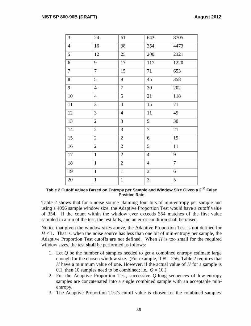
NIST SP 800-90B (DRAFT) August 2012
36
3 24 61 643 8705
4 16 38 354 4473
5 12 25 200 2321
6 9 17 117 1220
7 7 15 71 653
8 5 9 45 358
9 4 7 30 202
10 4 5 21 118
11 3 4 15 71
12 3 4 11 45
13 2 3 9 30
14 2 3 7 21
15 2 2 6 15
16 2 2 5 11
17 1 2 4 9
18 1 2 4 7
19 1 1 3 6
20 1 1 3 5
Table 2 Cutoff Values Based on Entropy per Sample and Window Size Given a 2-30
False Positive Rate
Table 2 shows that for a noise source claiming four bits of min-entropy per sample and
using a 4096 sample window size, the Adaptive Proportion Test would have a cutoff value
of 354. If the count within the window ever exceeds 354 matches of the first value
sampled in a run of the test, the test fails, and an error condition shall be raised.
Notice that given the window sizes above, the Adaptive Proportion Test is not defined for
H < 1. That is, when the noise source has less than one bit of min-entropy per sample, the
Adaptive Proportion Test cutoffs are not defined. When H is too small for the required
window sizes, the test shall be performed as follows:
1. Let Q be the number of samples needed to get a combined entropy estimate large
enough for the chosen window size. (For example, if N = 256, Table 2 requires that
H have a minimum value of one. However, if the actual value of H for a sample is
0.1, then 10 samples need to be combined; i.e., Q = 10.)
2. For the Adaptive Proportion Test, successive Q-long sequences of low-entropy
samples are concatenated into a single combined sample with an acceptable min-
entropy.
3. The Adaptive Proportion Test's cutoff value is chosen for the combined samples'

NIST SP 800-90B (DRAFT) August 2012
37
entropy estimate of QH bits2.
6.5.1.2.2.2 Running Adaptive Proportion Tests in Parallel
The performance tradeoffs between different window sizes means that choosing a single
window size requires either losing the ability to quickly discover large failures of the noise
source, or losing the ability to eventually discover subtle failures. A natural solution to this
is to run the Adaptive Proportion Test in parallel with different window sizes. For
example, it would be natural in some applications to use window sizes of both N = 64 and
N = 4096 to be used in parallel.
If two different window sizes are used, individual counters and cutoff values shall be
maintained for each window size.
6.5.1.3 Start-up and On-Demand Testing
Start-up testing is required to ensure that the entropy source components are working as
expected in order to verify that nothing failed since the last time the start-up tests were run.
This Recommendation requires that, at a minimum, the continuous tests be run at start-up;
note that the same requirements apply to the start-up tests as do the continuous tests: either
both the Repetition Count Test and the Adaptive Proportion test or their equivalent(s) (See
Section 10.0) shall be used as the start-up tests. At a minimum, the start-up tests shall
consist of one full cycle of the continuous tests to ensure that the continuous tests have had
an opportunity to verify that the device is working before it is used. Other tests in addition
to the continuous tests may also be run at start-up.
The parameters chosen for the start-up testing may be different than those used for the
continuous tests if power and memory are areas of concern while the entropy source is
starting up. Note that the entropy source shall not use noise source output for operational
purposes until it has passed the start-up tests. Therefore, more memory will be required,
depending on the parameters chosen, if the noise source outputs used during start-up
testing are intended to be used to create operational entropy source output since it will have
to be buffered until the start-up health tests have completed successfully. An alternative is
to throw out any noise source output used in start-up testing.
This Recommendation does not require that any particular on-demand testing be performed
during operation. However, it does require that the entropy source be capable of
performing on-demand health tests. Note that resetting, rebooting, or powering up are
acceptable methods for instituting an on-demand test if the procedure results in immediate
execution of the start-up tests.
2 Note that due to the conservative approach to entropy estimation it is possible to safely add together entropy
estimates, so that concatenating ten samples with one bit of min-entropy per sample yields a combined
sample with no less than ten bits of min-entropy.

NIST SP 800-90B (DRAFT) August 2012
38
6.5.2 Health Tests on the Conditioning Component
The role of the conditioning component is to reduce the bias that would otherwise be
present in the entropy source output and/or to ensure that the output bitstrings provide
entropy at an acceptable rate. The conditioning component will implement a deterministic
algorithm.
The functional requirements for the health tests of the conditioning component are:
1. The conditioning component shall be tested during start-up with known answer
tests necessary to establish that the conditioning component is working as designed.
2. The developer shall describe the health tests implemented for the conditioning
component to include the failure conditions covered by the tests chosen.
7.0 Validation Data and Documentation Requirements
Entropy source validation is necessary in order to obtain assurance that all relevant
requirements of this Recommendation are met. Validation consists of testing by an
NVLAP-accredited laboratory against the requirements of SP 800-90B, followed by a
review of the results by NIST’s CAVP and CMVP.
The validation of an entropy source presents many challenges. No other part of an RBG is
so dependent on technological and environmental differences. At the same time, the proper
operation of the entropy source is essential to the security of an RBG. This section presents
high-level requirements (on both developers and testers) for validation and provides a
method for mapping large samples into smaller bitstrings for situations in which it is
difficult to collect sufficient data for validation, given the size of the sample (see Section
7.2). The requirements below are intended to enable entropy source validation to help
justify why the entropy source can be relied upon.
7.1 General Validation Requirements
The entropy source consists of three components: the noise source, health tests, and an
optional conditioning component. The entropy source will have no more entropy than that
provided by the noise source, and as such, the noise source requires special attention
during validation testing. This is partly due to the fundamental importance of the noise
source (if it does not do its job, the entropy source will not provide the expected amount of
security), and partly because the probabilistic nature of its behavior requires more
complicated testing.
This section contains requirements for submitting an entropy source for [FIPS 140]
validation. Section 8.0 describes the testing strategy for noise sources, conditioned output,
and full-entropy sources. Section 9.0 details the specific validation tests.
The following are general requirements for validation testing.
1. Data Collection:

NIST SP 800-90B (DRAFT) August 2012
39
Data collection will be performed in one of two ways 1) by the developer with a
witness from the testing lab, or 2) by the testing lab itself. The entropy source
shall contain an interface that enables access to raw bits from the noise source
and conditioned outputs from the conditioning component (if utilized). This
interface shall consume the noise source outputs (i.e., these outputs shall not be
used for anything else once received by the interface). The interface shall be
accessible during validation testing but may be disabled, otherwise.
Data shall be collected from the noise source and conditioning component (if
available) under normal operating conditions (i.e., when it is reasonable to
expect entropy in the outputs).
Data collected from the noise source for validation testing shall be raw,
digitized, but otherwise unprocessed, sample values. NIST will provide
guidance as to the appropriate format of the data for input to the validation
tests.
One long dataset of at least 1,000,000 consecutive sample values obtained
directly from the noise source (i.e., raw and unprocessed samples) shall be
collected for validation3.
If a non-approved conditioning component is used, one long dataset of at least
1,000,000 consecutive conditioned output values shall be collected for
validation. Note that the data collected from the noise source for validation
may be used as input to the conditioning component for the collection of
conditioned output values.
For sample values consisting of more than a single bit, the developer shall
provide the tester with an ordered ranking of the bits in the sample values (see
Section 7.2).
Note that some tests will divide a dataset into multiple subsets of sample values; these
subsets will be called “data subsets”.
2. Validation Testing:
The continuous health tests shall be verified; the tester will verify that the
implemented tests detect the failure conditions detected by the Repetition Count
Test and Adaptive Proportion Test (See Section 6.5.1.2).
The tests in Section 9.0 will be run on all samples (noise source and non-
approved conditioning component output) submitted for testing; all data
collected will be tested as defined in Section 8.0.
3 Providing additional data beyond what is required will result in more accurate entropy estimates. Lack of
sufficient data for the tests in Section 9.0 yields lower entropy estimates due to the necessity of mapping
down the output values (see Section 7.2). It is recommended that, if possible, more data than is required be
collected for validation. However, it is assumed in subsequent text that only the required data has been
collected.

NIST SP 800-90B (DRAFT) August 2012
40
The developer shall indicate whether the noise source produces IID data or
non-IID data. This claim will be used in determining the test path followed
during validation. A claim of full-entropy will be interpreted as an IID claim.
The min-entropy estimate generated by the tests in Section 9.0 will be the value
at which the entropy source is validated. This entropy estimate will be in terms
of min-entropy per sample.
Full-entropy will be credited to an entropy source only after passing the tests
for IID data in this Recommendation (see Sections 9.1 and 9.2).
The tester will test all data as specified in Section 8.0, and will examine all
documentation and theoretical justifications submitted by the developer.
3. Documentation for Validation Testing (not for general consumption):
The developer shall provide documentation that describes the operation of the
entropy source to include how it works, how entropy is produced, and how to
obtain data from within the entropy source for testing purposes (i.e., from the
noise source and, if present, the conditioning component).
Documentation shall be provided so that the lab or vendor can perform (or
replicate) the collection process at a later time, if necessary. The collection
process shall not require advanced knowledge of the source or intrusive actions
that may alter the behavior of the entropy source (e.g., drilling into the device).
Documentation shall provide a technical argument for why the noise source can
support a defined entropy rate. This can be in broad terms of where the
unpredictability comes from and a rough description of the behavior of the
noise source (to show that it is reasonable to assume the behavior is stable).
Documentation shall describe the conditions under which the entropy source is
claimed to operate correctly (e.g., temperature range, voltages, system activity,
etc.). Analysis of the entropy source’s behavior at the edges of these conditions
shall be documented, along with likely failure modes.
A description of the health tests and the rationale for implementing those tests
shall be included. The developer shall provide source code for any tests
implemented as an alternative or in addition to those listed in this
Recommendation.
The developer shall provide a description of the output space of the noise
source, including its size, and shall specify the sample size from the noise
source - a fixed quantity for a given noise source.
For entropy sources containing a conditioning component, a description of the
conditioning component shall be provided that includes specification of the size
of the output blocks from the conditioning component.

NIST SP 800-90B (DRAFT) August 2012
41
7.2 Dealing with the Data Requirement for Noise Sources with Large Output Spaces
It is often the case that the data requirements for a test on noise source samples depend on
the number of possible different bitstrings from the source (i.e., the output space). For
example, consider two different noise sources, A and B. Source A outputs four-bit
samples, and thus has a possible total of 24 = 16 different outputs. Source B outputs 32-bit
samples, for a possible total of 232
different outputs.
In many cases, the variability in output that contributes to the entropy in a sample may be
concentrated among some portion of the bits in the sample. For example, consider a noise
source that outputs 32-bit high-precision clock samples that represent the time it takes to
perform some system process. Suppose that the bits in a sample are ordered in the
conventional way, so that the lower-order bits of the sample correspond to the higher
resolution measurements of the clock. It is easy to imagine that in this case, the low-order
bits would contain most of the variability. In fact, it would seem likely that some of the
high-order bits may be constantly 0. For this example, it would be reasonable to truncate
the 32-bit sample to a four-bit string by taking the lower four bits, and perform the tests on
the four-bit strings. Of course, it must be noted that in this case, a maximum of four bits of
min-entropy per sample could be credited to the noise source.
The description below provides a method for mapping the n-bit noise source samples,
collected as specified in Section 7.1, to strings of bit-length, m, where 𝑛 ≥ 𝑚. The
resulting strings can be used as input to tests that may have infeasible data requirements if
the mapping were not performed. Note that after the mapping is performed, the maximum
amount of entropy per n-bit sample is m bits.
In extreme cases, it is possible that there exists some dependency in the samples that is
controlled by the bits that have been discarded. If this is the case, any testing performed to
validate the entropy estimate of the processed samples may result in an over-estimate of
the entropy. To minimize this possibility, the mapping technique will not be performed
unless the sample bit-length is greater than can be handled by a particular test.
Given a noise source that produces n-bit samples, where n exceeds the bit-length that can
be handled by the test, the developer shall provide the tester with an ordered ranking of the
bits in the n-bit samples. The rank of ‘1’ shall correspond to the bit assumed to be
contributing the most entropy to the sample, and the rank of n shall correspond to the bit
contributing the least amount. If multiple bits contribute the same amount of entropy, the
ranks can be assigned arbitrarily among those bits. The following algorithm, or its
equivalent, shall be used to assign ranks.
Input: A noise source and corresponding statistical model with samples of the form
𝑋 = 𝑥1𝑥2 … 𝑥𝑛, where each xi is a bit.
Output: An ordered ranking of the bits x1 through xn, based on the amount of entropy that
each bit is assumed to contribute to the noise source outputs.
1. Set 𝑆 = {𝑥1, 𝑥2, … , 𝑥𝑛}.
2. For i = 1 to n:

NIST SP 800-90B (DRAFT) August 2012
42
a. Choose an output bit xj such that no other bit in S is assumed to contribute
more entropy to the noise source samples than xj.
b. Set rank(xj) = i.
c. Set 𝑆 = 𝑆 − {𝑥𝑗}.
Given the ranking, n-bit samples are mapped to m-bit strings by simply taking the m-bits of
greatest rank in order (i.e., bit 1 of the m-bit string is the bit from an n-bit sample with rank
1, bit 2 of the m-bit string is the bit from an n-bit sample with rank 2, … and bit m of the
m-bit string is the bit from an n-bit sample with rank m).
Note that for the tests in Section 9.0, a reference to a sample in the dataset will be
interpreted as a reference to the m-bit string of the sample when the test necessitates
processing the dataset as specified in this section.
8.0 Entropy Source Testing Strategy
8.1 General Noise Source Entropy Testing Strategy
The most basic requirement for any entropy source is estimating the min-entropy correctly.
A min-entropy estimate for the entropy source is calculated from the data submitted for
testing, as defined in Section 7.1. As shown in Figure 3, the test track is initially
influenced by the developer’s claim that the data source does or does not produce IID data.
Both tracks result in a min-entropy estimate, but use different information to determine the
entropy in a dataset, based upon whether or not the data is IID. Claims for full-entropy
imply an entropy source produces IID data; any claim for full-entropy will be interpreted
as an IID claim.
1. If the data is claimed to be IID, a full set of shuffling and statistical tests is run on
the data to verify that the data is IID (see Section 9.1); the claim is verified if there
is no evidence that the data is not IID.
2. If the results from the tests in Section 9.1 verify that the data is IID (via a lack of
evidence to the contrary), the min-entropy of the noise source is estimated using the
tests in Section 9.2. This estimate will be used as the validated min-entropy
estimate for a noise source that produces IID data.
3. Alternatively, if there is no IID claim or if the tests in Section 9.1 do not support
such a claim, a set of five conservative entropy tests are performed on the non-IID
data to obtain the min-entropy estimate. The five tests for non-IID data in Section
9.3 will result in the calculation of five different entropy estimates. By selecting
the minimum of all estimates calculated by the tests, a worst-case estimate of the
entropy is obtained, and this conservative estimate will be used as the min-entropy
estimate for a noise source that does not produce IID data.
4. Following the generation of an entropy estimate, the datasets are subjected to the
sanity checks defined in Section 9.4. These tests are designed to discover major
failures in the design and gross overestimates of entropy by the test suite. Failure

NIST SP 800-90B (DRAFT) August 2012
43
to pass the sanity checks means that the entropy source fails testing. Entropy will
not be credited to that entropy source.
At this point, if the entropy source does not include a conditioning component, given that
the entropy source components pass the tests, the entropy source will be validated at the
determined min-entropy per noise source sample. Otherwise, see Section 8.2.

NIST SP 800-90B (DRAFT) August 2012
44
Figure 3: Flowchart Depicting the Entropy Testing Strategy
Submitted with
an IID or Full
Entropy claim?
Estimate the min-
entropy with the
IID ‘bins’ test
(Section 9.2).
Estimate the min-
entropy with tests
for non-IID data
(Section 9.3).
yes
No
Perform Sanity Checks on
data/entropy estimate submitted
(Section 9.410.0).
No
Yes
Yes (may be Full Entropy)
Validated at entropy
estimate calculated above.
Verify IID with shuffling and
statistical tests (Section 9.1).
Is the data IID? No
Pass? Testing Fails. No
entropy estimate
awarded.
(not Full Entropy)

NIST SP 800-90B (DRAFT) August 2012
45
8.2 Entropy Source Testing Strategy for Conditioned Output
There are various methods for designing a conditioning component for an entropy source.
One such method involves using an approved cryptographic algorithm/function to
condition the noise source outputs. If an approved algorithm, discussed in Section 6.4.1,
is used as the conditioning component, validation testing on the output from the
conditioning component using the appropriate tests in Section 9.0 will not be performed4.
If a non-approved algorithm is used as the conditioning component, validation testing on
the output from the conditioning component using the tests in Section 9.1 will be
performed. Any conditioned output must be IID.
1. If a conditioning component is implemented in the entropy source, use the results of
noise source testing to determine the amount of entropy provided in each input to the
conditioning component (i.e., the amount of entropy in the input is the assessed amount
of entropy per sample from the noise source times the number of samples provided for
the conditioning component input).
a. If the conditioning component is approved, then:
i. Given assurance of correct implementation of the approved algorithm, the
entropy estimate for each output of the conditioning component is
min(outlen, entropy_in), where outlen is the length of the output from the
conditioning component, and entropy_in is the amount of entropy per bit in
the input to the conditioning component. Note that it is acceptable to
truncate the cryptographic output. If this is done, the entropy estimate is
reduced to a proportion of the output (e.g., if there are 6 bits of entropy in
an 8 bit output and the output is truncated to 6 bits, then the entropy is
reduced by ¼ to 4.5 bits).
ii. If validation testing of the approved algorithm indicates that it has not been
implemented correctly, the conditioning component will be treated as not
approved.
b. If the conditioning component is not approved, then:
i. Determine the input/output ratio, R. Most conditioning functions will take
in more bits than they output. In some cases, the ratio of input to output bits
will be fixed. If this is the case, the input/output ratio will be determined by
simply calculating the number of bits of input needed to produce a given
number of output bits. On the other hand, some conditioning components
may take an indeterminate number of input bits to produce a given number
of output bits (e.g. von Neumann unbiasing, where the number of bits of
output depends not only on the number of bits of input, but on the actual
values of the input bits.) In this case, the ratio of input bits to output bits
4 Note, however, that these algorithms are subject to other validation testing to obtain assurance of correct
implementation and obtain their approval rating.
NIST SP 800-90B (DRAFT) August 2012
46
will be estimated by processing 1,000,000 bits of noise source data through
the conditioning component and observing the number of bits of output.
ii. Run the tests in Section 9.1 on the output of the conditioning component.
Any conditioned output must be IID; a full set of shuffling and statistical
tests is run on the data to verify that the data is IID. The sample size of the
conditioned output is the size of the output space of the non-approved
conditioning component (e.g., if MD5 is the conditioning component, the
sample size is 128 bits).
a. The claim is verified if there is no evidence that the data is not IID
and testing continues.
i. The min-entropy of the conditioned output is estimated using
the test in Section 9.2.
ii. Let S be the entropy estimate for the noise source (i.e. the
number of bits of entropy per bit of noise source output.) as
determined by the noise source validation tests. Let E be the
entropy estimate for the conditioned output values, and let R
be the input/output ratio of the conditioning component.
Since the conditioning component cannot increase the
entropy, it must be the case that S/R ≥ E. If this condition is
not met, the entropy estimate E will be adjusted to be equal
to S/R.
b. If the tests in Section 9.1 do not support the IID claim, then the
entropy source fails validation, and testing is terminated.
iii. Following the generation of an entropy estimate, the data is subjected to the
sanity checks defined in Section 9.4. These tests are designed to discover
major failures in the design and gross overestimates of entropy by the test
suite. Failure to pass the sanity checks means that the entropy source fails
testing. Entropy will not be credited to that entropy source.
At this point, given that the conditioned output is found to be IID and the components have
passed the sanity checks, the entropy source will be validated at the min-entropy per
conditioned output, E, computed above.
8.3 Entropy Source Testing Strategy for Full Entropy Sources
Claims for full-entropy imply that a noise source or an entropy source produces IID data;
any claim for full-entropy will be interpreted as an IID claim. There are two basic options
for full-entropy: full-entropy with no conditioning component, and full-entropy through
implementation of an approved conditioning component. Entropy sources that implement
a non-approved conditioning component will not be validated as full-entropy sources.
1. If full entropy is claimed, the data must be IID. A full set of shuffling and
statistical tests is run on the data to verify that the data is IID (see Section 9.1).

NIST SP 800-90B (DRAFT) August 2012
47
a. If the noise source passes the IID tests in Section 9.1 (i.e., there is no
evidence that the data is not IID), then testing continues. The min-entropy
of the noise source is estimated using the tests in Section 9.2.
i. For full-entropy sources with no conditioning component: Credit
for full-entropy will be given only if the data is verified to be IID,
and a full-entropy estimate is produced by the tests in this
Recommendation.
ii. For full-entropy sources with an approved conditioning component:
Credit for full-entropy will be given only if the data is verified to be
IID, and the noise source input used to derive the W -bit full entropy
conditioned output has at least 2W bits of min-entropy (see Section
6.4).
b. If the noise source does not pass the IID tests in Section 9.1, then full
entropy is not provided and the entropy source will not be validated as a
full-entropy source. Validation may continue, however, using the non-IID
path.
2. Following the generation of an entropy estimate, the datasets are subjected to the
sanity checks defined in Section 9.4. These tests are designed to discover major
failures in the design and gross overestimates of entropy by the test suite. Failure
to pass the sanity checks means that the entropy source fails testing. Entropy will
not be credited to that entropy source.
At this point, given that the entropy source components have passed the tests, the entropy
source will be validated at the determined min-entropy per sample.
8.4 Entropy Source Testing Strategy for the Health Test Component
Entropy sources that do not implement the Repetition Count Test and the Adaptive
Proportion Test shall include alternative continuous tests that detect the same failure
conditions. The tester will determine the equivalence of the alternative test(s) as described
in Section 10.0.
Submitters of entropy sources for validation testing are required to provide a dataset of at
least a million samples drawn from their noise source for validation testing. The testing of
the submitter’s alternative test(s) for equivalent functionality also requires a dataset; the
same dataset may be used for both noise source validation testing and the testing of
equivalent functionality of the continuous health tests.
The tests work as follows:
1. A dataset, D, taken from the noise source is modified to simulate a particular kind
of failure that the Repetition Count or Adaptive Proportion Test will detect with
very high probability. Note that a different simulated failure is used (and thus a
different altered dataset is created) for each test, although the same “original”
dataset may be used.
NIST SP 800-90B (DRAFT) August 2012
48
2. The alternative test(s) is applied to this modified dataset, D'. If the simulated
failure is detected, then the alternative test is assumed to provide equivalent
functionality.
If these tests for equivalent functionality fail, then the requirement on the health test
component is not met and the entropy source will not be validated.
9.0 Tests for Determining Entropy Provided by Entropy Sources
One of the essential requirements of an entropy source is the ability to reliably create
random outputs. To ensure that sufficient entropy is input to a DRBG (see [SP 800-90C]
for DRBG constructions), the amount of entropy produced per noise source sample must
be determined. This Section describes generic tests that will be used to test the noise
source and, when non-approved methods are used, the conditioning component as well
(see Section 8.2).
The tests described in this Section are appropriate for a wide range of noise sources.
Because these tests are generic, they are aimed at catching serious problems and are not
meant to address all possible types of sources or all failure conditions.
The test descriptions in this Section are written for an accredited testing laboratory,
although the tests are also useful for entropy source developers.
9.1 Determining if the Data is IID
9.1.1 General Discussion
This section describes tests appropriate for a wide range of noise sources and non-
approved conditioning components in which each sample is drawn from the same
distribution, and its probability of occurrence is independent of any other value sampled.
A noise source or conditioning component that meets this requirement is known as IID
(independent and identically distributed). These tests are designed to find evidence that the
data is IID by testing the dataset against the hypothesis that the distribution of samples is
IID. These tests are used as a check on the validity of the developer’s claim that an IID
source has been submitted; the testing consists of the shuffling tests defined in Section
9.1.2, and the statistical tests defined in Section 9.1.3. If the tests do not disprove the IID
claim (i.e., the dataset passes the IID testing), further testing continues under the
assumption that the noise source outputs IID data (see Figure 3). A failure of any of the
shuffling or statistical tests in Section 9.1 results in a cessation of IID testing and a switch
to tests for non-IID data (see Section 9.3).
9.1.2 Shuffling Tests on Independence and Stability
Given the null hypothesis that the samples follow an IID distribution, a shuffled version of
a dataset should be just as likely to have occurred as the original dataset that was produced.
The original dataset’s test score is expected to be drawn from the same distribution as the
scores of the shuffled datasets; an original dataset test score of unusually high or low rank

NIST SP 800-90B (DRAFT) August 2012
49
(see Step 2c below) is expected to occur very infrequently. However, if the null hypothesis
is not true (i.e., the samples do not follow an IID distribution), then some test scores may
be very different for the original and shuffled datasets.
A dataset created as specified in Section 7.1 will be divided into ten non-overlapping data
subsets of equal size, i.e., for a dataset consisting of N samples, each data subset would be
10
N samples in length. Each of these data subsets will be tested to determine if the
samples follow an IID distribution.
Shuffling tests detect a deviation of the noise source or conditioning component
distribution from independent and stable behavior using the following strategy:
1. Several statistical scores are calculated. Certain behavior is not consistent with the
expected model of an independent, stable distribution for the samples and is
expected to be associated with unusually low or high values for the test scores. The
following scores are computed:
Compression score: one score per data subset (see Section 9.1.2.1),
Over/Under Runs score: two scores per data subset (see Section 9.1.2.2),
Excursion score: one score per data subset (see Section 9.1.2.3),
Directional Runs score: three scores per data subset (see Section 9.1.2.4),
Covariance score: one score per data subset (see Section 9.1.2.5), and
Collision score: three scores per data subset (see Section 9.1.2.6).
2. The following steps are performed on each of the ten data subsets being tested:
a. The scores are computed for the (original) data subset, yielding a vector of J
scores.
b. The following steps are repeated 1,000 times for the data subset:
i. The values in the (original) data subset are shuffled (i.e., permuted),
using a pseudorandom number generator as specified by the Fisher-
Yates shuffle [Knuth].
ii. The scores are computed for the shuffled data subset, yielding a
vector of J scores, where J is the number of scores for a given test
on a single dataset (see step 1 above).
iii. The scores are stored in a list.
c. For each of the corresponding scores for a data subset (e.g., all the first
scores resulting from the directional runs test), the original data subset’s
score (from step 2a) is ranked, in terms of how it compares to the scores of
the shuffled data subsets. For example, if the original data subset’s score is
lower than the score of all the shuffled data subsets, the rank of the original
data subset’s score is 1, and the scores for all the other shuffled data subsets
would have a higher rank. If the original data subset’s score is higher than
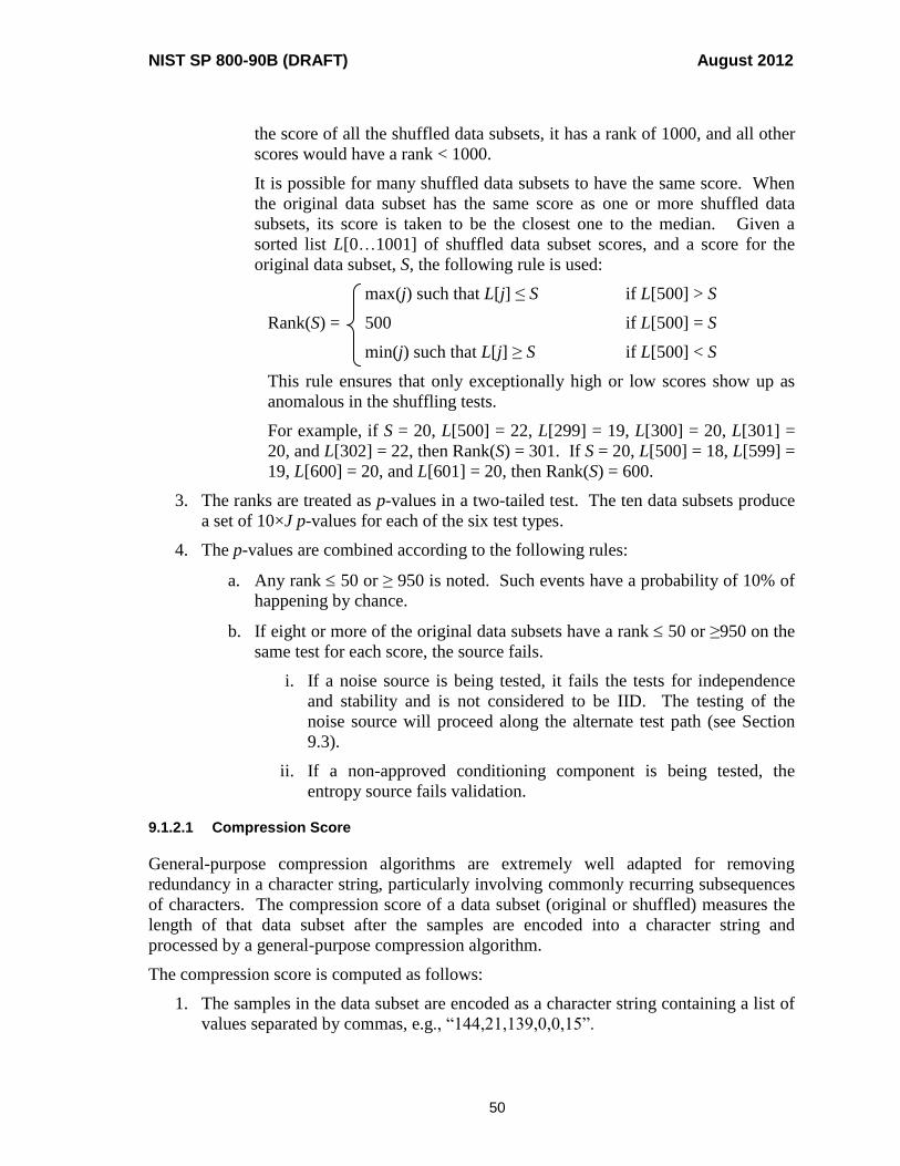
NIST SP 800-90B (DRAFT) August 2012
50
the score of all the shuffled data subsets, it has a rank of 1000, and all other
scores would have a rank < 1000.
It is possible for many shuffled data subsets to have the same score. When
the original data subset has the same score as one or more shuffled data
subsets, its score is taken to be the closest one to the median. Given a
sorted list L[0…1001] of shuffled data subset scores, and a score for the
original data subset, S, the following rule is used:
max(j) such that L[j] ≤ S if L[500] > S
Rank(S) = 500 if L[500] = S
min(j) such that L[j] ≥ S if L[500] < S
This rule ensures that only exceptionally high or low scores show up as
anomalous in the shuffling tests.
For example, if S = 20, L[500] = 22, L[299] = 19, L[300] = 20, L[301] =
20, and L[302] = 22, then Rank(S) = 301. If S = 20, L[500] = 18, L[599] =
19, L[600] = 20, and L[601] = 20, then Rank(S) = 600.
3. The ranks are treated as p-values in a two-tailed test. The ten data subsets produce
a set of 10×J p-values for each of the six test types.
4. The p-values are combined according to the following rules:
a. Any rank 50 or ≥ 950 is noted. Such events have a probability of 10% of
happening by chance.
b. If eight or more of the original data subsets have a rank 50 or ≥950 on the
same test for each score, the source fails.
i. If a noise source is being tested, it fails the tests for independence
and stability and is not considered to be IID. The testing of the
noise source will proceed along the alternate test path (see Section
9.3).
ii. If a non-approved conditioning component is being tested, the
entropy source fails validation.
9.1.2.1 Compression Score
General-purpose compression algorithms are extremely well adapted for removing
redundancy in a character string, particularly involving commonly recurring subsequences
of characters. The compression score of a data subset (original or shuffled) measures the
length of that data subset after the samples are encoded into a character string and
processed by a general-purpose compression algorithm.
The compression score is computed as follows:
1. The samples in the data subset are encoded as a character string containing a list of
values separated by commas, e.g., “144,21,139,0,0,15”.
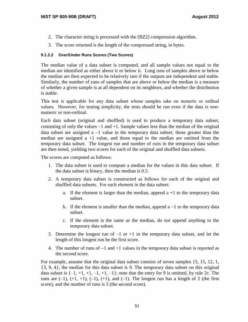
NIST SP 800-90B (DRAFT) August 2012
51
2. The character string is processed with the [BZ2] compression algorithm.
3. The score returned is the length of the compressed string, in bytes.
9.1.2.2 Over/Under Runs Scores (Two Scores)
The median value of a data subset is computed, and all sample values not equal to the
median are identified as either above it or below it. Long runs of samples above or below
the median are then expected to be relatively rare if the outputs are independent and stable.
Similarly, the number of runs of samples that are above or below the median is a measure
of whether a given sample is at all dependent on its neighbors, and whether the distribution
is stable.
This test is applicable for any data subset whose samples take on numeric or ordinal
values. However, for testing simplicity, the tests should be run even if the data is non-
numeric or non-ordinal.
Each data subset (original and shuffled) is used to produce a temporary data subset,
consisting of only the values 1 and +1. Sample values less than the median of the original
data subset are assigned a 1 value in the temporary data subset; those greater than the
median are assigned a +1 value, and those equal to the median are omitted from the
temporary data subset. The longest run and number of runs in the temporary data subset
are then noted, yielding two scores for each of the original and shuffled data subsets.
The scores are computed as follows:
1. The data subset is used to compute a median for the values in this data subset. If
the data subset is binary, then the median is 0.5.
2. A temporary data subset is constructed as follows for each of the original and
shuffled data subsets. For each element in the data subset:
a. If the element is larger than the median, append a +1 to the temporary data
subset.
b. If the element is smaller than the median, append a 1 to the temporary data
subset.
c. If the element is the same as the median, do not append anything to the
temporary data subset.
3. Determine the longest run of –1 or +1 in the temporary data subset, and let the
length of this longest run be the first score.
4. The number of runs of 1 and +1 values in the temporary data subset is reported as
the second score.
For example, assume that the original data subset consists of seven samples {5, 15, 12, 1,
13, 9, 4}; the median for this data subset is 9. The temporary data subset on this original
data subset is {–1, +1, +1, –1, +1, –1}; note that the entry for 9 is omitted, by rule 2c. The
runs are (–1), (+1, +1), (–1), (+1), and (–1). The longest run has a length of 2 (the first
score), and the number of runs is 5 (the second score).

NIST SP 800-90B (DRAFT) August 2012
52
9.1.2.3 Excursion Score
The excursion score detects when a sequence of extremely high or low values clusters
together in the data subset. This indicates a distribution that may fail to be stable or
independent. Both high and low excursion scores are of interest. High scores represent
clusters of unusually high/low values occurring together; low scores represent some
process that prevents unusually high/low values from clustering together even as often as
would be expected by chance.
The excursion score is meaningful if the average value of the samples is meaningful (e.g.,
an average can be computed on the dataset values). In a large number of cases in which
the sample value is a count or a digitized value, the average of the dataset values can be
computed. However, for test simplicity, the tests should be run even if an average cannot
be computed.
The excursion score is a measure of how far the running sum of sample values deviates
from its expected value at each point in the data subset. If the data subset is s0, s1, s2,...,
and the mean of the sample values is , then the excursion at position i is s0+s1+...+si –
i×. The score returned is the maximum absolute value of any excursion in the data
subset.
The score is computed as follows, where = the mean of the values in the data subset.
1. For j = 1 to
10
N (where
10
N is the length of the data subset in samples):
dj = the absolute value of (the sum of the first j samples – j×)
2. The score returned is the largest of the dj values.
For example, if the data subset is {2, 15, 4, 10, 9}, then = 8. d1 = |2-8| = 6; d2 = |(2+15) –
(28)| = 1; d3 = |(2+15+4) – (38)| = 3; d4 = |(2+15+4+10) – (48)| = 1; d5 =
|(2+15+4+10+9) – (58)| = 0. Therefore, the score is 6, the highest value for dj.
9.1.2.4 Directional Runs Scores (Three scores)
Many physical processes are best understood in terms of their derivatives. If the first
derivative alternates signs between samples, then a large number of short directional runs
will be noted.
Each data subset (original and shuffled) is used to generate a temporary data subset that is
one element shorter than the original (or non-temporary) data subset. The temporary data
subset contains an indication of whether the first value in each pair of elements is less than,
equal to, or greater than the second element in the pair. If the first element is less than the
second element, then a +1 is appended to the temporary data subset; if the two elements are
equal, then a 0 is appended to the temporary data subset; otherwise the first element is
greater than the second element, and a 1 is appended to the temporary data subset. For
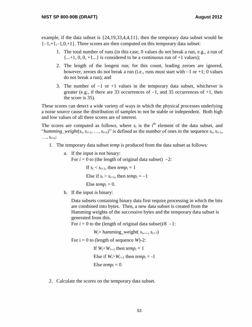
NIST SP 800-90B (DRAFT) August 2012
53
example, if the data subset is {24,19,33,4,4,11}, then the temporary data subset would be
{1,+1,1,0,+1}. Three scores are then computed on this temporary data subset:
1. The total number of runs (in this case, 0 values do not break a run, e.g., a run of
{...+1, 0, 0, +1...} is considered to be a continuous run of +1 values);
2. The length of the longest run; for this count, leading zeroes are ignored,
however, zeroes do not break a run (i.e., runs must start with 1 or +1; 0 values
do not break a run); and
3. The number of 1 or +1 values in the temporary data subset, whichever is
greater (e.g., if there are 33 occurrences of 1, and 35 occurrences of +1, then
the score is 35).
These scores can detect a wide variety of ways in which the physical processes underlying
a noise source cause the distribution of samples to not be stable or independent. Both high
and low values of all three scores are of interest.
The scores are computed as follows, where si is the ith
element of the data subset, and
“hamming_weight(si, si+1, …, si+n)” is defined as the number of ones in the sequence si, si+1,
…, si+n:
1. The temporary data subset temp is produced from the data subset as follows:
a. If the input is not binary:
For i = 0 to (the length of original data subset) 2:
If si < si+1, then tempi = 1
Else if si > si+1, then tempi = 1
Else tempi = 0.
b. If the input is binary:
Data subsets containing binary data first require processing in which the bits
are combined into bytes. Then, a new data subset is created from the
Hamming weights of the successive bytes and the temporary data subset is
generated from this.
For i = 0 to the (length of original data subset)/8 1:
Wi= hamming_weight( si,..., si+7)
For i = 0 to (length of sequence W)-2:
If Wi<Wi+1 then tempi = 1
Else if Wi>Wi+1 then tempi = -1
Else tempi = 0
2. Calculate the scores on the temporary data subset.
NIST SP 800-90B (DRAFT) August 2012
54
Example of a non-binary data subset {2, 2, 2, 5, 7, 7, 9, 3, 1, 4, 4}: The temporary data
subset is {0, 0, +1, +1, 0, +1, 1, 1, +1, 0}. There are three runs: (+1, +1, 0, +1), (1, 1)
and (+1, 0), so the first score is three. The longest run has a length of four (the second
score). Since there are four “1” values, and two “1” values, the third score is four.
Example of a binary data subset: The bytes produced by step 1b (represented as
hexadecimal values) are {a3, 57, 3f, 42, bd}. The hamming weights are {4, 5, 6, 2, 6}. The
temporary data subset is {+1, +1, 1, +1}. There are three runs: (+1, +1), (1) and (+1), so
the first score is three. The longest run has a length of two (the second score). Since there
are three “+1” values and one “1” value, the third score is three.
9.1.2.5 Covariance Score
Many of the likely ways that a noise source can fail to be IID involve dependencies
between nearby samples. The chi-square test of independence (see Section 9.1.3.1), and
the compression score (see Section 9.1.2.1) are effective at detecting repeating patterns of
particular values (e.g., strings of sample values that occur more often than would be
expected by chance if the noise source were IID), but will not, in general, detect
relationships between the numeric values of successive samples (e.g., high sample values
usually being followed by low sample values). The covariance score will detect such
relationships.
The behavior of the covariance score is well-understood for bivariate normal distributions.
However, any linear relationship between the successive pairs of values will affect this
score, and so the covariance is expected to be different (larger or smaller) for the original
data subsets than for the shuffled data subsets, if such a relationship exists.
The covariance of two variables is defined as the expected value of their product, minus
the product of their expected values. The covariance is a common statistical measure of
whether two variables have a linear relationship. The covariance score is computed over
each pair of the data subset S, so that s0 is paired with s1, s1 with s2, etc.
The score is computed as follows, where si is the ith
element of the data subset, numbered
from zero, and there are a total of
10
N samples in the data subset:
1. count = 0
2. = the mean of s0, s1, s2, ..., sN/10-1.
3. For i = 1 to
10
N:
count = count + (si )(si1 )
4. Score =
110
N
count.
NIST SP 800-90B (DRAFT) August 2012
55
For example, if the data subset is {15, 2, 6, 10, 12}, then there are five samples in the data
subset, and the mean is 9. For i=1, count = (29)(159) = 42; for i=2, count = 42 +
(69)(29) = 21; for i=3, count = 21 + (109)(69) = 24; for i=4, count = 24 +
(129)(109) = 21. The score is (21/4) = 5.
9.1.2.6 Collision Score (Three scores)
A natural measure of how much entropy is in a variable comes from the number of times it
must be sampled before the first duplicate value (“collision”) occurs. A source that is IID
can be expected to have the same behavior with respect to the number of samples that
occur before a collision occurs as its shuffled variants. By contrast, a source in which the
probability of the most likely value changes over time is likely to require fewer samples to
find a collision in its unshuffled outputs than in its shuffled outputs.
The collision score measures the number of successive sample values until a duplicate (a
“collision”) is seen. A single data subset will normally have many times this number of
values, and so many such collisions can be sought in different parts of the data subset.
Starting at the beginning of the data subset, samples are examined until a duplicate is
found. The number of samples examined is noted, and then a new search for duplicates
starts at the next element in the data subset. This continues until the whole data subset has
been checked. The set of numbers of samples examined is then used to compute three
scores: the smallest number, the average, and the largest number.
In the case of binary data, a data subset consisting of binary data is converted into a
sequence of 8-bit bytes before being subjected to this test, so that each sequence of eight
bits in the original data subset becomes one byte in the modified data subset. The modified
data subset is then subjected to the above process to compute collision scores. Note that
both the (original) data subset and each shuffled data subset are separately modified by this
process. Also note that the length of this modified data subset is
80
N because of this
process, whereas the length of the original binary data subset and data subsets that do not
consist of binary data have a length of
10
N.
The scores are computed as follows:
1. Counts is a list of counts of samples needed to see a duplicate; the list is initially
empty.
2. pos = 0
3. While pos < (the length of the data subset):
a. Find the smallest j such that spos .. spos+j contains one duplicate value.
i. If no such j exists, break out of the while loop.
b. Add j to the list of Counts.
c. pos = pos + j + 1

NIST SP 800-90B (DRAFT) August 2012
56
4. Return the following values as scores: the minimum value in the Counts list, the
average of all values in the Counts list, and the maximum value in the Counts list.
For example, if the data subset is {2, 1, 1, 2, 0, 1, 0, 1, 1, 2}, the length of the data subset is
10. If the first “2” is at position 0, then the first collision occurs when j = 2 (i.e., samples 1
and 2 are both ones). Disregarding the first three samples in the data subset, the next
sequence to be examined is {2, 0, 1, 0, 1, 1, 2}, the collision for this new sequence occurs
when j = 3 (i.e., samples 1 and 3 of this second sequence are both zeros). The third
sequence to be examined is {1, 1, 2}; the collision for this third sequence occurs when j =
1 (i.e., samples 0 and 1 are both ones). The final sequence to be examined is {2}, for which
there are no collisions. The counts collected for this test occur when j = 2, j = 3, and j = 1.
The first score returned is 1 (the minimum count value); the second score is 2 (the average
of the count values); the third score is 3 (the maximum value of the count values).
9.1.3 Specific Statistical Tests
9.1.3.1 Chi-Square Test
Sample values are limited to a fixed range of possibilities. If the requirements on the noise
source and non-approved conditioning component to be IID are met, then the distribution
of these values can be seen as an independent category distribution (a multinomial
distribution, in which the individual sample values have no meaningful relationship.) The
chi-square test can be used to test whether a particular dataset fits a particular multinomial
distribution.
Chi-square tests can be used to check whether a dataset of samples follows some expected
distribution, and also whether two or more datasets follow the same distribution. It should
be noted that there are some distributions for which a chi-square test cannot be performed
because the data requirements are too great. This occurs when the output samples have a
large number of possible values, none with very high probability. In these cases, two
options are available: 1) more data than required in Section 7.1 should be submitted (or
collected) such that the test can be executed, or 2) if additional data cannot be obtained, the
chi-square test can be skipped, since it will not be possible to perform the test. If the test is
not performed due to lack of data, the rest of the validation testing will continue as
specified.
Two different types of chi-square tests are employed for validating a noise source and non-
approved conditioning components: a test for independence, and a test for goodness-of-fit.
The independence test attempts to discover dependencies in probabilities between
successive samples in the (entire) dataset submitted for testing as specified in Section 7.1
(see Section 9.1.3.1.1 for non-binary data and Section 9.1.3.1.3 for binary data); the
goodness-of-fit test attempts to discover a failure to follow the same distribution in the ten
data subsets produced from the (entire) dataset submitted for testing (see Section 9.1.3.1.2
for non-binary data and Section 9.1.3.1.4 for binary data).

NIST SP 800-90B (DRAFT) August 2012
57
9.1.3.1.1 Testing Independence for Non-Binary Data
For this test, the (entire) dataset submitted for testing, as defined in Section 7.1 is used to
estimate the probability of each possible value occurring (i.e., each value that a single
sample could assume). The dataset is used to estimate the probabilities for each possible
value of x that could occur. The occurrences of pairs of such values in the dataset are then
checked against their theoretical probability of occurrence.
Let p(xi) equal the estimated probability that value xi will occur in any given sample. Let
List1 contain a list of (xi, xj) pairs that is expected to occur at least five times, and List2
contain a list of (xi, xj) pairs that is expected to occur less than five times. Let E(xi, xj) be
the expected number of occurrences for the (xi, xj) pairs in List1, and Eother be the total of
the expected number of occurrences of the entries in List2.
Informally, the chi-square test for independence is carried out as follows:
1. Determine p(xi) for each possible output value in the dataset by counting the
number of occurrences of each xi, and dividing by the length of the dataset.
2. Determine pmax = the maximum probability that occurs in the dataset.
3. Let N = the number of samples in the dataset.
4. Count the number of parameters to be estimated. Let q = 1; start with 1 because the
catch-all category probability will be estimated.
a. For each p(xi ) :
If p(xi )pmax ≥ 5/N, let q = q + 1.
q now contains the number of parameters that are estimated in this test.
Now, determine the number of bins.
b. If q=1, then the test halts with no result--there are no pairs with high enough
probability to run the test on. This means that the dataset is too small to run
this test on this source distribution.
5. The sets of pairs of values that are expected to occur at least five times or less than
five times are constructed, as follows:
a. Set List1 and List2 to empty sets.
b. Eother = 0.
c. For each possible pair of values (xi, xj), including (xi, xi):
If p(xi)p(xj)N ≥ 5:
i. Add the (xi, xj) pair to List1.
ii. Let E(xi, xj) = p(xi)p(xj)N.
Else:
iii. Add the (xi, xj) pair to List2.
iv. Eother = Eother + p(xi)p(xj)N.

NIST SP 800-90B (DRAFT) August 2012
58
6. Verify that enough degrees of freedom are obtained to run the test. If not, this test
has no result; the test may be omitted or more data may be requested.
a. Let w = the number of pairs that appear in List1.
b. If w+1-q < 1: halt the test with no result – there is not enough data to run the
test properly.
7. Compute the chi-square score:
a. X1 = 0.
b. For each pair (xi, xj) in List1:
i. Obs(xi, xj) = the number of occurrences of this pair of values in the
dataset.
ii. X1 = X1 + (E(xi, xj) – Obs(xi, xj))2/E(xi, xj).
c. X2 = 0.
d. For each pair (xi, xj) in List2:
i. Obs(xi, xj) = the number of occurrences of this pair in the dataset.
ii. X2 = X2 + Obs(xi, xj).
e. X = X1 + (X2 Eother)2/Eother.
X is a chi-square value. Compare X with the 0.001 cutoff value for a chi-square with w+1-
q degrees of freedom. If X is larger than this cutoff value, the dataset fails the test; this is
strong evidence that sample values in the sequence are not independent. A high chi-square
score indicates a lack of independence, and a p-value less than 0.001 causes this test to fail
9.1.3.1.2 The Test for Goodness of Fit for Non-Binary Data
For this test, the (entire) dataset, as defined in Section 7.1, is used to estimate the expected
number of occurrences of each sample value in each of the ten subsets of the dataset.
These values are then used to test the hypothesis that the values have the same probabilities
of occurring in each of the ten data subsets.
Let xi be a possible output (i.e., a possible sample). Let E(xi) = the expected number of
occurrences of xi in any one data subset. Let List3 and List4 be lists of the values of xi. Let
Eother = the sum of the E(xi) for each xi in List4.
Informally, the chi-square test for goodness of fit is carried out as follows:
1. Determine E(xi) for each xi. This is the total number of occurrences of xi in the
entire dataset, divided by ten.
2. Let List3 be the list of values of xi, such that E(xi) ≥ 5.
3. Let List4 be the list of values of xi, such that E(xi) <5.
4. Eother = 0.
5. For each xi in List4:

NIST SP 800-90B (DRAFT) August 2012
59
Eother = Eother + E(xi).
6. Let X1= 0.
7. For each of the ten data subsets:
a. Let Obs (xi) be the observed number of occurrences of xi in the data subset.
b. For each xi in List3 (i.e., each xi that is expected to occur at least five times):
X 1= X1 + (Obs(xi) E(xi))2/E(xi).
c. Obsother = the number of occurrences of values in List4 in the data subset.
d. X = X1 + (Obsother Eother)2/Eother.
The final total value X is a chi-square variable, with 9|L| degrees of freedom, where L is the
length of List3, plus 1 (i.e., the number of values with expected value ≥ 5, plus 1). A p-
value of less than 0.001 means that one or more of the ten data subsets do not fit the
distribution determined from the (entire) dataset, and the test fails.
9.1.3.1.3 Testing Independence for Binary Data
If the binary source is IID, then each bit appears with the same probability everywhere in
the dataset. This means that the probability of each k-bit string is the probabilities of each
of its successive bits, multiplied together. This test checks to see if these k-bit strings have
the expected probability over the whole dataset. If nearby bits are not independent, then
the expected probabilities of k-bit strings derived from bit probabilities will be wrong for
the whole dataset, and the chi-square score will be much larger than expected.
This test can be applied to binary data to test the independence of the bits in the dataset. In
order to do this, successive bits must be grouped together as follows:
1. Let C0 be the count of zeros in the dataset, and C1 be the count of ones.
2. Let Cx be whichever of those two is smaller. That is, Cx = min(C0, C1).
3. Let N be the total number of bits in the dataset.
4. Let k = 2
5. While k < 12 and (Cx/N)k > 5/N:
k = k + 1
6. k = k – 1
At the end of this process, 2 k < 12. Construct a modified dataset from the dataset as
follows:
new_dataset[i] = dataset[ki .. (k+1)i-1]
That is, each successive k bits of the dataset becomes a new element in new_dataset. The
expected probabilities of each value in the dataset, and a chi-square score are computed as
follows:
1. p = C1/N (the probability of getting a one bit in the dataset).

NIST SP 800-90B (DRAFT) August 2012
60
2. S = 0.0.
3. For value = 0 to 2k-1:
a. W = hamming_weight(value) (i.e., number of ones in value)
b. prob(value) = pW
(1-p)k-W
.
(That is, the probability of each value is estimated, based on the bit
probabilities.)
c. E(value) = prob(value)N/k.
d. Let Cvalue = the number of times that value appears in new_dataset.
e. S = S + (Cvalue-E(value))2/E(value).
The final total value S is a chi-square variable, with 2k-1 degrees of freedom. Compare S
with the 0.001 cut-off value for a chi-square with 2k-1 degrees of freedom. A high chi-
square score indicates a lack of independence; if S is larger than this cut-off value, the
dataset fails the test.
9.1.3.1.4 Testing for Stability of Distribution in Binary Data
Given an estimate of the bit probability p for a one over the (entire) dataset, a goodness-of-
fit test can be used to verify that the probability is stable across the ten individual data
subsets as follows:
1. Let p be the probability that a bit in the (original) dataset is a one. This is
computed as:
p = (number of one bits in the dataset/N).
2. Let Nd be the length of each of the ten individual data subsets (i.e.,
10
N).
3. Let Ed = pNd.
4. S = 0.0
5. For d = 1 to 10:
a. Cd = the number of ones in data subset d.
b. S = S + (Cd - Ed)2/ Ed .
S is a chi-square variable with 9 degrees of freedom. The test fails if S is larger than the
critical value at .001, which is 27.9.
9.1.3.2 Other Statistical Tests
Other statistical tests may be added in the future.

NIST SP 800-90B (DRAFT) August 2012
61
9.2 Estimating the Min-Entropy of IID Sources
Similar to a ‘bins’ test, this test estimates the entropy provided by an IID source, based on
the number of observations of the most common output value. Estimating entropy in an
IID source is a simple process: the most common value in the dataset described in Section
7.1 is found and counted. This is used to produce a 99% upper bound on the probability of
the most common value, pmax, and that upper bound is used to produce a lower bound
estimate of min-entropy per sample of the source.
Simply counting the most common value introduces a small bias in favor of more
conservative estimates, as it tends to overestimate pmax in some distributions. However,
in practice, this bias is small enough to have little importance5.
It is important to note that the estimate is not meaningful when the source is not IID. The
test is performed as follows:
Given a dataset with N samples.
1. Find the most common value in the dataset.
2. Count the occurrences of that value, and call the result CMAX.
3. Let pmax = CMAX/N.
4. Calculate CBOUND = CMAX + 2.3√𝑁𝑝𝑚𝑎𝑥(1 − 𝑝𝑚𝑎𝑥).
5. Let H = –log2(CBOUND/N).
6. Let W be the number of bits in each sample of the dataset (i.e., the size of the
sample).
7. min(W, H) is the lower-bounded entropy estimate.
For example, if the dataset is {0, 1, 1, 2, 0, 1, 2, 2, 0, 1, 0, 1, 1, 0, 2, 2, 1, 0, 2, 1}, the most
common value is “1”, CMAX = 8, and pmax = 0.4.
CBOUND = 8 + 2.3√4.8 = 13.04.
H = –log(0.652) = 0.186.
W = 3.
min(3, 0.186) = 0.186.
9.3 Estimating the Min-Entropy of non-IID Sources
9.3.1 General Discussion
Many viable noise sources fail to produce independent outputs. Moreover, some sources
may have dependencies that are beyond the ability of the tester to address. To derive any
utility out of such sources, a diverse and conservative set of entropy tests are required.
5 Experimentally, uniform eight-bit random values lose less than a bit from their entropy estimates, while
uniform 16-bit random values lose a little more than two bits from their entropy estimates.
NIST SP 800-90B (DRAFT) August 2012
62
Testing sources with dependencies in time and/or state may result in overestimates of
entropy instead of underestimates. However, a large, diverse battery of tests minimizes the
probability that such a source’s entropy is greatly overestimated.
The battery of tests presented in this section will be performed on noise sources
determined to be non-IID by the testing performed in Section 9.1, and any noise source
submitted for testing without an IID claim6. The five tests, each designed to compute a
different statistic on the samples, provide information about the structure of the data:
collision, collection, compression, Markov, and frequency. While the tests (except for the
Markov) were originally designed for application to independent outputs, the tests have
performed well when applied to data with dependencies. Given empirical evidence and the
confidence level of the tests, their application to non-IID data will produce valid, although
conservative, entropy estimates.
9.3.2 Testing Summary
The working assumption for these tests is that a probability distribution describes the
output of a random noise source, but that the probability distribution is unknown. The goal
of each test is to reveal information about the unknown distribution, based on a statistical
measurement. The presented entropy tests define a set of IID probability distributions that
contain the unknown distribution; the entropy is conservatively estimated by minimizing
over this set of distributions. The five tests fall into two types: the first type bounds the
entropy of a noise source, based on a statistical measurement with a prescribed amount of
confidence, while the second type constructs a set of probability distributions based on the
distance to the measured statistic within a prescribed confidence level.
For the tests defined in this section, a confidence level of 95%, denoted by , is used; the
confidence interval encompasses the true value of the measured statistic 95% of the time.
9.3.3 The Collision Test
9.3.3.1 Test Overview
The collision test measures the mean time to the first collision in a dataset. The goal of the
collision statistic is to estimate the probability of the most-likely state, based on the
collision times. The test will produce a low entropy estimate for noise sources that have
considerable bias toward an output or state (i.e., the mean time until a collision is relatively
short), while producing longer mean times to collision results in higher entropy estimates.
This test yields a lower bound on the entropy present with a prescribed confidence level
when the samples are independent. Dependencies in the sample data may cause an
overestimate of the entropy of the data. In practice, a slight overestimate is resolved by
selecting the minimum entropy estimate from all the tests as the expected entropy provided
by the noise source.
6 Any conditioned output must be IID, so the tests in this section will not be performed on conditioning
component output (see Section 8.2).

NIST SP 800-90B (DRAFT) August 2012
63
9.3.3.2 Implementation Summary
Given a dataset from the noise source, step through the dataset (i.e., sample by sample)
until any observed value is repeated. Record the number of steps to the observed collision.
Beginning from that point, step through the remaining samples until another observed
value is repeated. Continue this process at least 1000 times until the end of the dataset is
reached, generating a sequence of collision times, where the collision time corresponds to
the number of samples observed before a collision occurs. The observation of 1000
collisions is dependent on the sample size, and may not be possible for sources with large
samples. Given the data requirement specified in Section 7.1, an observation of 1000
collisions in sources with samples larger than 20 bits will not be feasible. For example, a
source that produces 32-bit outputs would need approximately 226
samples to observe 1000
collisions. As an alternative for noise sources with large sample sizes, the method in
Section 7.2 for mapping noise source outputs together7 (based on a ranking of the bits in
the output) may be implemented, or additional data may be collected for testing purposes.
This will enable the observation of at least 1000 collision events regardless of the sample
size. One of these options will be enforced, based on the data provided, so that the test can
be run and 1000 collision events observed.
Once the end of the dataset is reached, calculate the mean collision time of the differences
in the sequence of collision times. Then, determine the probability distribution that has the
minimum possible entropy for the calculated mean collision time. For this distribution, the
min-entropy is calculated and returned as the lower bound on the entropy that is present.
9.3.3.3 Collision Test Details
Given a dataset {s1, s2, …, sN}, of noise or entropy source observations.
1. Beginning with s1, step through the dataset until any observed value is repeated;
i.e., find the smallest j such that si = sj, for some i with 1 ≤ 𝑖 < 𝑗.
2. Define a sequence t. Set t0 = 0, t1 = j.
3. Set v = 1.
4. Starting with sample j, step through the remaining samples, sj+1, sj+2, …, sN, until
there is a k and an l such that sk = sl, with 𝑗 < 𝑘 < 𝑙.
5. v = v + 1.
6. Define tv = l.
7. Set j = l.
8. Repeat steps 4-7 until the end of the dataset is reached. A sequence {t0, t1, t2, …, tv}
is generated. If v < 1000, the noise source outputs will be mapped down based on
the ranking provided, and the data will be retested.
7 Note that mapping outputs together will result in potentially smaller entropy estimates than if sufficient data
was tested.

NIST SP 800-90B (DRAFT) August 2012
64
9. Calculate the sample mean, µ, and the sample standard deviation, σ, of the
differences of collision times, ti.
𝜇 =∑ (𝑡𝑖 − 𝑡𝑖−1)𝑣
𝑖=1
𝑣
𝜎 = √∑ (𝑡𝑖 − 𝑡𝑖−1)2𝑣
𝑖=1
𝑣− 𝜇2
10. Compute the lower-bound of the confidence interval for the mean based on a
normal distribution with confidence level α:
�̅� = 𝜇 −1.96𝜎
√𝑣.
11. Define a one-parameter family of probability distributions parameterized by p, Pp:
𝑃𝑝(𝑖) = {
𝑝 𝑖𝑓 𝑖 = 01 − 𝑝
𝑛 − 1𝑜𝑡ℎ𝑒𝑟𝑤𝑖𝑠𝑒
where n is the number of states in the output space.
12. Using a binary search, solve for the parameter p, such that p
E the expected value
of the statistic applied to Pp, equals .
𝐸𝑃𝑝(𝑆) = 𝑝𝑞−2 (1 +
1
𝑛(𝑝−1 − 𝑞−1)) 𝐹(𝑞) − 𝑝𝑞−1
1
𝑛(𝑝−1 − 𝑞−1)
where
𝑞 =1 − 𝑝
𝑛 − 1,
and
𝐹(1 𝑧⁄ ) = Γ(𝑛 + 1, 𝑧)𝑧−𝑛−1𝑒−𝑧 .
13. The min-entropy is the negative logarithm of the parameter, p:
min-entropy = –log2(p).
NIST SP 800-90B (DRAFT) August 2012
65
9.3.4 The Partial Collection Test
9.3.4.1 Test Overview
The partial collection test computes the entropy of a dataset based on how many distinct
values in the output space are observed; it yields low entropy estimates for output streams
that contain a small number of distinct output values, and yields high entropy estimates for
output streams that diversify quickly. The partial collection test provides a reasonable
estimate for sources with output values that appear with higher probability than others in
the output space. An advantage of the partial collection test over the traditional collection
test8 is that it finishes in finite time, since the test estimates the entropy of a source, given
the number of distinct values in a set of samples in the dataset.
It should be noted that the partial collection test will only produce an accurate entropy
estimate if the size of the output space is known. For example, consider a noise source that
outputs four-bit samples, but only two of those bits are ever influenced/used by the noise
source. This reduces the number of possible output values and limits the output space.
Instead of 24 = 16 possible values, this source only produces 2
2 = 4 different values. A
search for all 16 possibilities will be fruitless, and the entropy will be greatly overestimated
by this test. Therefore, the output space of the noise source or an indication of values that
never appear in the output from the noise source shall be provided by the developer for
validation testing.
Given the data requirement specified in Section 7.1, samples larger than 10 bits will not be
feasible. As an alternative for noise or entropy sources with large sample sizes, the method
in Section 7.2 for mapping noise source outputs together9 (based on a ranking of the bits in
the output) may be implemented, or additional data may be collected for testing purposes.
Based on the data provided for validation, one of these options will be enforced such that
the test can be run and 500 events observed.
9.3.4.2 Implementation Summary
Partition the dataset into non-overlapping subsets of size n (where n is the size of the
output space). The partial collection test computes the number of distinct values in each
subset of n samples. Once all subsets have been parsed, calculate the mean number of
distinct values in each subset of n samples. Then, determine the probability distribution
that has the minimum possible entropy for the calculated mean number of distinct values.
For this distribution, the min-entropy is calculated and returned as the lower bound on the
entropy that is present.
8 The traditional collection test measures the expected number of samples that must be generated to produce
every possible output, and as such, could potentially never terminate.
9 Note that mapping outputs together will result in potentially smaller entropy estimates than if sufficient data
was tested.
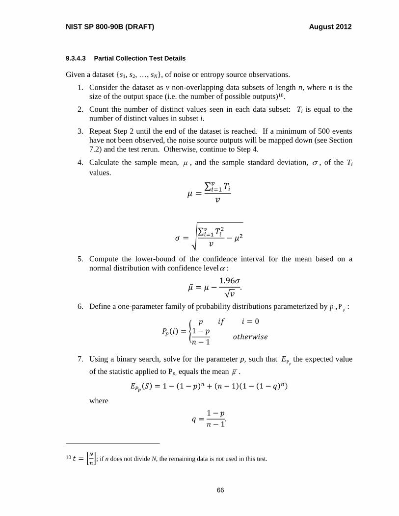
NIST SP 800-90B (DRAFT) August 2012
66
9.3.4.3 Partial Collection Test Details
Given a dataset {s1, s2, …, sN}, of noise or entropy source observations.
1. Consider the dataset as v non-overlapping data subsets of length n, where n is the
size of the output space (i.e. the number of possible outputs)10.
2. Count the number of distinct values seen in each data subset: Ti is equal to the
number of distinct values in subset i.
3. Repeat Step 2 until the end of the dataset is reached. If a minimum of 500 events
have not been observed, the noise source outputs will be mapped down (see Section
7.2) and the test rerun. Otherwise, continue to Step 4.
4. Calculate the sample mean, , and the sample standard deviation, , of the Ti
values.
𝜇 =∑ 𝑇𝑖
𝑣𝑖=1
𝑣
𝜎 = √∑ 𝑇𝑖
2𝑣𝑖=1
𝑣− 𝜇2
5. Compute the lower-bound of the confidence interval for the mean based on a
normal distribution with confidence level :
�̅� = 𝜇 −1.96𝜎
√𝑣.
6. Define a one-parameter family of probability distributions parameterized by p ,p :
𝑃𝑝(𝑖) = {
𝑝 𝑖𝑓 𝑖 = 01 − 𝑝
𝑛 − 1𝑜𝑡ℎ𝑒𝑟𝑤𝑖𝑠𝑒
7. Using a binary search, solve for the parameter p, such that p
E the expected value
of the statistic applied to Pp, equals the mean .
𝐸𝑃𝑝(𝑆) = 1 − (1 − 𝑝)𝑛 + (𝑛 − 1)(1 − (1 − 𝑞)𝑛)
where
𝑞 =1 − 𝑝
𝑛 − 1.
10 𝑡 = ⌊𝑁
𝑛⌋; if n does not divide N, the remaining data is not used in this test.
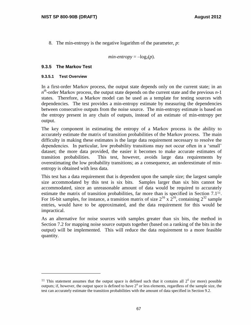
NIST SP 800-90B (DRAFT) August 2012
67
8. The min-entropy is the negative logarithm of the parameter, p:
min-entropy = –log2(p).
9.3.5 The Markov Test
9.3.5.1 Test Overview
In a first-order Markov process, the output state depends only on the current state; in an
nth
-order Markov process, the output state depends on the current state and the previous n-1
states. Therefore, a Markov model can be used as a template for testing sources with
dependencies. The test provides a min-entropy estimate by measuring the dependencies
between consecutive outputs from the noise source. The min-entropy estimate is based on
the entropy present in any chain of outputs, instead of an estimate of min-entropy per
output.
The key component in estimating the entropy of a Markov process is the ability to
accurately estimate the matrix of transition probabilities of the Markov process. The main
difficulty in making these estimates is the large data requirement necessary to resolve the
dependencies. In particular, low probability transitions may not occur often in a ‘small’
dataset; the more data provided, the easier it becomes to make accurate estimates of
transition probabilities. This test, however, avoids large data requirements by
overestimating the low probability transitions; as a consequence, an underestimate of min-
entropy is obtained with less data.
This test has a data requirement that is dependent upon the sample size; the largest sample
size accommodated by this test is six bits. Samples larger than six bits cannot be
accommodated, since an unreasonable amount of data would be required to accurately
estimate the matrix of transition probabilities, far more than is specified in Section 7.111.
For 16-bit samples, for instance, a transition matrix of size 216
x 216
, containing 232
sample
entries, would have to be approximated, and the data requirement for this would be
impractical.
As an alternative for noise sources with samples greater than six bits, the method in
Section 7.2 for mapping noise source outputs together (based on a ranking of the bits in the
output) will be implemented. This will reduce the data requirement to a more feasible
quantity.
11 This statement assumes that the output space is defined such that it contains all 26 (or more) possible
outputs; if, however, the output space is defined to have 26 or less elements, regardless of the sample size, the
test can accurately estimate the transition probabilities with the amount of data specified in Section 9.2.
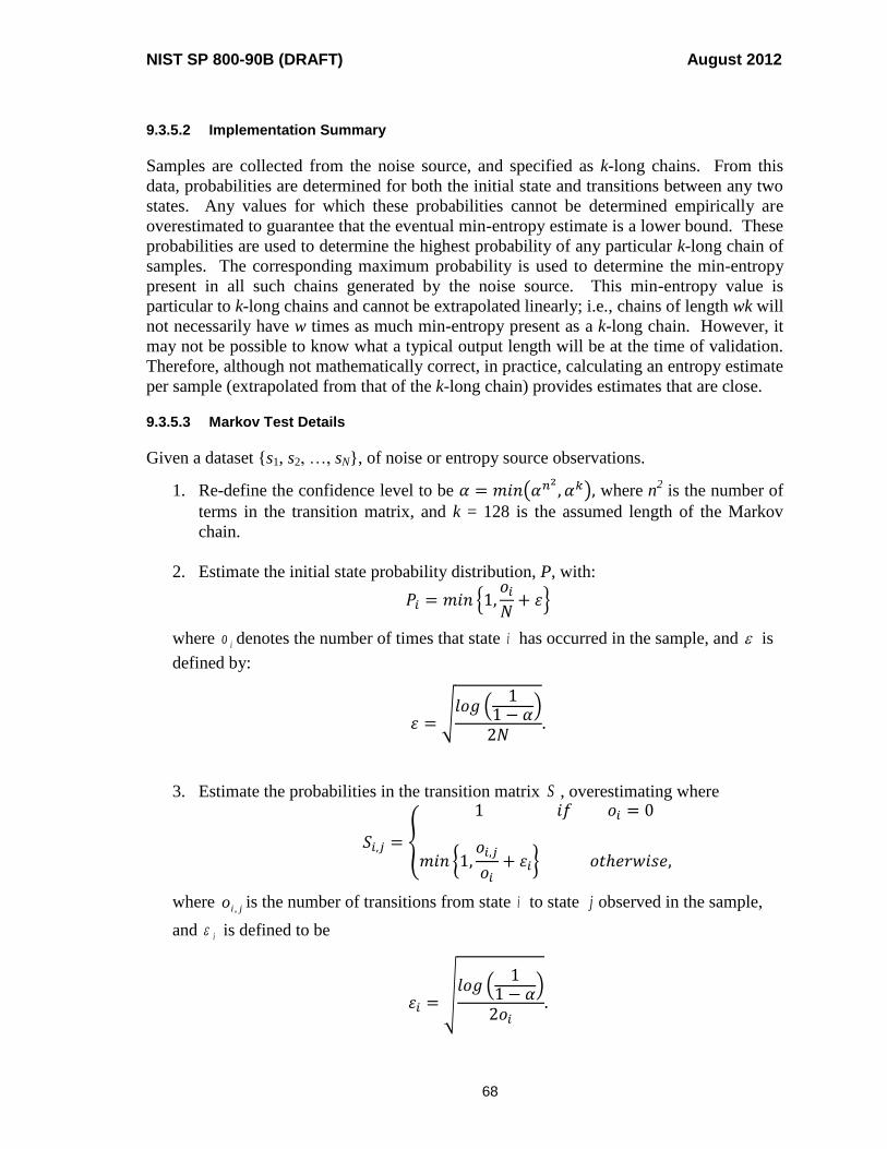
NIST SP 800-90B (DRAFT) August 2012
68
9.3.5.2 Implementation Summary
Samples are collected from the noise source, and specified as k-long chains. From this
data, probabilities are determined for both the initial state and transitions between any two
states. Any values for which these probabilities cannot be determined empirically are
overestimated to guarantee that the eventual min-entropy estimate is a lower bound. These
probabilities are used to determine the highest probability of any particular k-long chain of
samples. The corresponding maximum probability is used to determine the min-entropy
present in all such chains generated by the noise source. This min-entropy value is
particular to k-long chains and cannot be extrapolated linearly; i.e., chains of length wk will
not necessarily have w times as much min-entropy present as a k-long chain. However, it
may not be possible to know what a typical output length will be at the time of validation.
Therefore, although not mathematically correct, in practice, calculating an entropy estimate
per sample (extrapolated from that of the k-long chain) provides estimates that are close.
9.3.5.3 Markov Test Details
Given a dataset {s1, s2, …, sN}, of noise or entropy source observations.
1. Re-define the confidence level to be 𝛼 = 𝑚𝑖𝑛(𝛼𝑛2, 𝛼𝑘), where n
2 is the number of
terms in the transition matrix, and k = 128 is the assumed length of the Markov
chain.
2. Estimate the initial state probability distribution, P, with:
𝑃𝑖 = 𝑚𝑖𝑛 {1,𝑜𝑖
𝑁+ 𝜀}
where io denotes the number of times that state i has occurred in the sample, and is
defined by:
𝜀 =√𝑙𝑜𝑔 (
11 − 𝛼)
2𝑁.
3. Estimate the probabilities in the transition matrix S , overestimating where
𝑆𝑖,𝑗 = {
1 𝑖𝑓 𝑜𝑖 = 0
𝑚𝑖𝑛 {1,𝑜𝑖,𝑗
𝑜𝑖+ 𝜀𝑖} 𝑜𝑡ℎ𝑒𝑟𝑤𝑖𝑠𝑒,
where jio , is the number of transitions from state i to state j observed in the sample,
and i is defined to be
𝜀𝑖 = √𝑙𝑜𝑔 (
11 − 𝛼)
2𝑜𝑖.
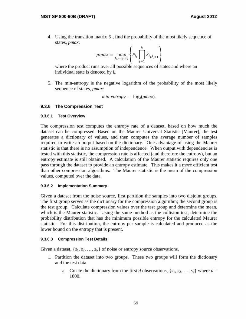
NIST SP 800-90B (DRAFT) August 2012
69
4. Using the transition matrix S , find the probability of the most likely sequence of
states, pmax.
𝑝𝑚𝑎𝑥 = max𝑖1…𝑖𝑙…𝑖𝑘
{𝑃𝑖𝑙∏ 𝑆𝑖𝑗,𝑖𝑗+1
𝑘
𝑗=1
}
where the product runs over all possible sequences of states and where an
individual state is denoted by il.
5. The min-entropy is the negative logarithm of the probability of the most likely
sequence of states, pmax:
min-entropy = –log2(pmax).
9.3.6 The Compression Test
9.3.6.1 Test Overview
The compression test computes the entropy rate of a dataset, based on how much the
dataset can be compressed. Based on the Maurer Universal Statistic [Maurer], the test
generates a dictionary of values, and then computes the average number of samples
required to write an output based on the dictionary. One advantage of using the Maurer
statistic is that there is no assumption of independence. When output with dependencies is
tested with this statistic, the compression rate is affected (and therefore the entropy), but an
entropy estimate is still obtained. A calculation of the Maurer statistic requires only one
pass through the dataset to provide an entropy estimate. This makes it a more efficient test
than other compression algorithms. The Maurer statistic is the mean of the compression
values, computed over the data.
9.3.6.2 Implementation Summary
Given a dataset from the noise source, first partition the samples into two disjoint groups.
The first group serves as the dictionary for the compression algorithm; the second group is
the test group. Calculate compression values over the test group and determine the mean,
which is the Maurer statistic. Using the same method as the collision test, determine the
probability distribution that has the minimum possible entropy for the calculated Maurer
statistic. For this distribution, the entropy per sample is calculated and produced as the
lower bound on the entropy that is present.
9.3.6.3 Compression Test Details
Given a dataset, {s1, s2, …, sN} of noise or entropy source observations.
1. Partition the dataset into two groups. These two groups will form the dictionary
and the test data.
a. Create the dictionary from the first d observations, {s1, s2, …, sd} where d =
1000.

NIST SP 800-90B (DRAFT) August 2012
70
b. The remaining 𝑣 = 𝑁 − 𝑑 − 1 observations, {sd+1, …, sN}, will be the test
data.
2. Initialize the dictionary.
a. Beginning with s1, step through the dictionary sequence.
b. Record each unique observation and the index of observation.
c. When any observed value is repeated, update the index of observation with
the most recent index value (the larger index value).
3. Run the test data against the dictionary created in Step 2.
a. Beginning with 𝑠𝑑+1, step through the test data.
b. Determine if the value of the observation is contained in the dictionary.
i. If the value is in the dictionary, calculate and record the difference
between the current observation index and the recorded index in the
dictionary as Ai, where i is the current index. Update the dictionary
with the index of the most recent observation.
ii. If the value is not in the dictionary, add that value to the dictionary,
and record the index of this first observation.
4. Repeat Step 3 until the end of the test data has been reached.
5. Calculate the sample mean, , and the sample standard deviation, , of the
following values:
(𝑙𝑜𝑔2(𝐴𝑖))𝑖=𝑑+1
𝑁
where the Ai are the calculated differences from Step 3b.
𝜇 =∑ 𝑙𝑜𝑔2𝐴𝑖
𝑁𝑖=𝑑+1
𝑣
𝜎 = √∑ (𝑙𝑜𝑔2𝐴𝑖)2𝑁
𝑖=𝑑+1
𝑣− 𝜇2
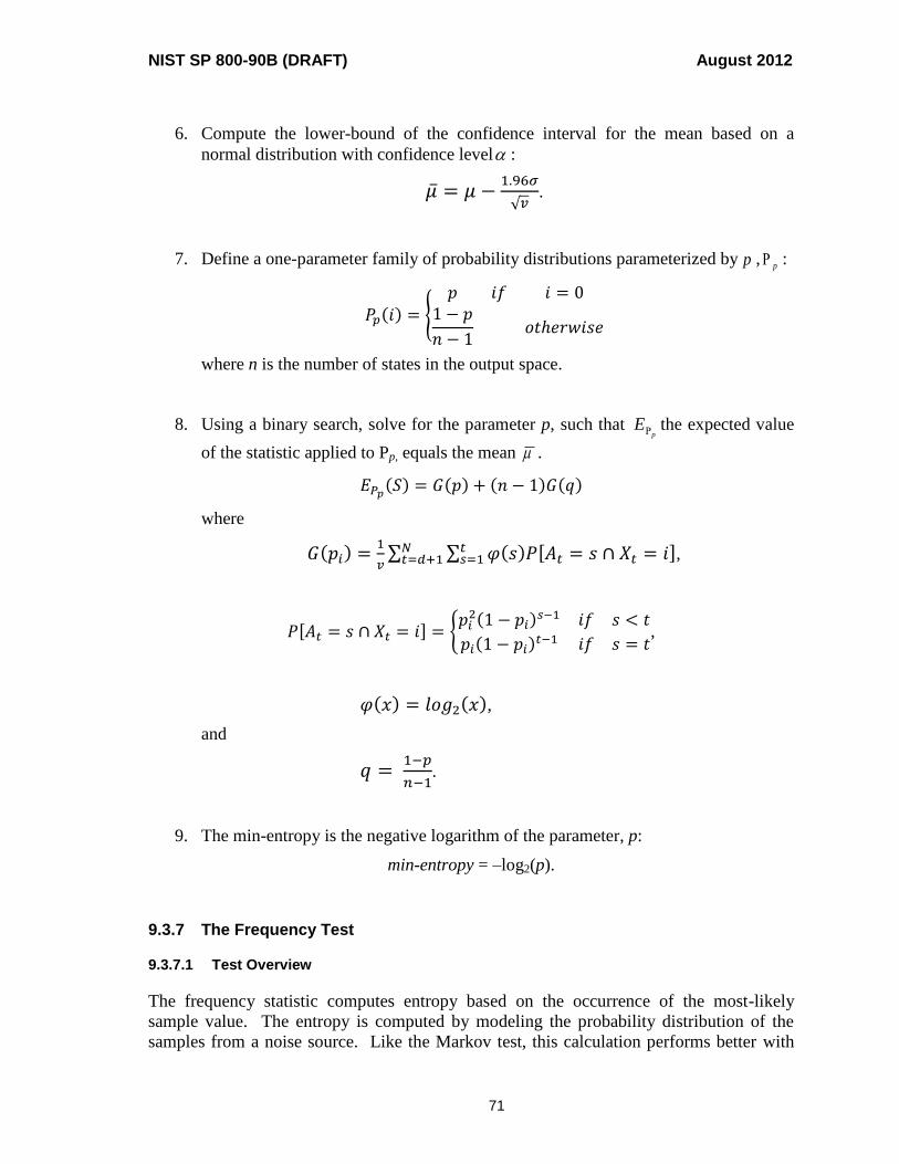
NIST SP 800-90B (DRAFT) August 2012
71
6. Compute the lower-bound of the confidence interval for the mean based on a
normal distribution with confidence level :
�̅� = 𝜇 −1.96𝜎
√𝑣.
7. Define a one-parameter family of probability distributions parameterized by p ,p :
𝑃𝑝(𝑖) = {
𝑝 𝑖𝑓 𝑖 = 01 − 𝑝
𝑛 − 1𝑜𝑡ℎ𝑒𝑟𝑤𝑖𝑠𝑒
where n is the number of states in the output space.
8. Using a binary search, solve for the parameter p, such that p
E the expected value
of the statistic applied to Pp, equals the mean .
𝐸𝑃𝑝(𝑆) = 𝐺(𝑝) + (𝑛 − 1)𝐺(𝑞)
where
𝐺(𝑝𝑖) =1
𝑣∑ ∑ 𝜑(𝑠)𝑃[𝐴𝑡 = 𝑠 ∩ 𝑋𝑡 = 𝑖]𝑡
𝑠=1𝑁𝑡=𝑑+1 ,
𝑃[𝐴𝑡 = 𝑠 ∩ 𝑋𝑡 = 𝑖] = {𝑝𝑖
2(1 − 𝑝𝑖)𝑠−1 𝑖𝑓 𝑠 < 𝑡
𝑝𝑖(1 − 𝑝𝑖)𝑡−1 𝑖𝑓 𝑠 = 𝑡
,
𝜑(𝑥) = 𝑙𝑜𝑔2(𝑥),
and
𝑞 = 1−𝑝
𝑛−1.
9. The min-entropy is the negative logarithm of the parameter, p:
min-entropy = –log2(p).
9.3.7 The Frequency Test
9.3.7.1 Test Overview
The frequency statistic computes entropy based on the occurrence of the most-likely
sample value. The entropy is computed by modeling the probability distribution of the
samples from a noise source. Like the Markov test, this calculation performs better with

NIST SP 800-90B (DRAFT) August 2012
72
more data – the more data provided, the more accurate the frequency calculations, since
low probability values may not appear often, or at all, in ‘small’ datasets. This test,
however, ignores/overestimates unlikely sample values and, therefore, does not require
large amounts of data. In fact, this test will provide a conservative estimate of entropy
based on whatever data is collected. As a result, an underestimate of min-entropy is
obtained with less data.
9.3.7.2 Implementation Summary
Given a dataset from the noise source, step through the dataset, keeping track of the
number of times that each sample value is observed. Record the occurrence of each value
and continue the process until the end of the dataset. Once the end of the dataset is
reached, determine the most likely sample value, based on the frequency counts gathered.
The min-entropy frequency statistic is the negative logarithm of the probability of the most
likely sample value.
9.3.7.3 Frequency Test Details
Given a dataset, {s1, s2, …, sN}, and the confidence level α:
1. Beginning with s1, step through the dataset, keeping track of the number of times a
value is observed, counti, for all i=1...n, where n is the number of possible output
values.
2. Calculate ε from the specified confidence level, α, and the number of observations
in the dataset.
𝜀 = √𝑙𝑜𝑔 (
11 − 𝛼
)
2𝑁
3. Determine the probability of the most likely observation value, pmax (the value
with the largest frequency of occurrence):
𝑝𝑚𝑎𝑥 = max𝑖=1..𝑛 (𝑐𝑜𝑢𝑛𝑡𝑖
𝑁).
4. The min-entropy is the negative logarithm of the sum of ε and the frequency of the
probability of the occurrence of the most likely state, pmax:
min-entropy = –log2(pmax + ε).

NIST SP 800-90B (DRAFT) August 2012
73
9.4 Sanity Checks Against Entropy Estimates
This section identifies tests that provide an opportunity to discover major failures that may
have undermined the entropy estimates generated in the more extensive test suites.
9.4.1 Compression Sanity Check
The compression test is intended to determine whether the entropy estimates for the noise
source and conditioning component are so incorrect that a general-purpose compression
algorithm is able to encode the sequence of samples in fewer bits per sample than is
required by the entropy estimate computed during validation testing. The Burrows-
Wheeler compression algorithm as implemented in the BZ2 software package will be used
[BZ2].
If the min-entropy of a dataset is estimated to be H bits, then no compression algorithm
should be capable, in general, of encoding that dataset in fewer than H bits.
By nature, general-purpose compression algorithms like Burrows-Wheeler will perform
poorly, compared to what is attainable in encoding specialized data, especially independent
values. Thus, a single failed test is an indication that the entropy estimate is deeply flawed.
Let S be a collected dataset defined in Section 7.1. Divide S into ten equal-length, non-
overlapping data subsets S1, …, S10. Let Si be one of the ten data subsets, and let H be the
entropy estimate for the data source, as calculated in Section 9.2 or Section 9.3 (depending
upon the test track taken). The test is performed as follows on the ten data subsets of
samples:
For i = 1 to 10:
1. EncodeS = the encoding of Si as a string12.
2. C = compress(EncodeS).
3. Len = the length of C in bits.
4. If 𝐿𝑒𝑛 < 𝐻 ⌊𝑁
10⌋, the dataset fails the test.
If the test fails for even one of the ten data subsets, it is likely that the entropy estimate is
inaccurate.
9.4.2 Collision Sanity Check
9.4.2.1 General Description
The min-entropy can be used to provide a bound on the probability of seeing a collision in
many trials because the collision entropy (Renyi entropy of second order) is bounded by
12 EncodeS consists of representing the sequence of samples as a character string containing their decimal
values separated by commas. Thus, a sequence (3, 1, 4, 1, 5, 9) becomes “3, 1, 4, 1, 5, 9”.

NIST SP 800-90B (DRAFT) August 2012
74
the min-entropy. There are many ways in which a noise source might suffer rare,
intermittent failures that would lead to an occasional repeated sequence that should, given
the entropy estimates, have an extremely low probability of occurring. This kind of
problem will be detected by the collision sanity check, while it might not be detected by
any other test.
The collision sanity check offers a chance to notice a particular kind of gross overestimate
of entropy, in which sequences of samples with some useful amount of entropy (for
example, 30 bits) repeat more often than expected.
This test may be applied to any noise source, using a dataset as specified in Section 7.1.
9.4.2.2 Testing Noise Sources With an Entropy Estimate per Sample
For datasets whose entropy estimate is in terms of H bits of entropy per sample, the testing
is performed as follows:
1. Using the complete dataset collected as specified in Section 7.1, determine the size
of the ‘tuples’ to be examined for collisions. This test will examine each
successive b-tuple of samples from the dataset. To determine b, numerically solve
using the following equation for b:
b = Round((2 log2(N/b) -1)/H).
The formula is derived as follows: Given N samples in the dataset, the dataset can
be divided into (N/b) non-overlapping b-tuples. The number of times each b-tuple
occurs in the dataset must be counted; since there are ⌊𝑁
𝑏⌋ b-tuples, there are about
(⌊𝑁
𝑏⌋)
2
2 potential collisions of b-tuples. Since each b-tuple has Hb bits of entropy,
the expected number of b-tuple collisions is:
2−𝐻𝑏(⌊
𝑁
𝑏⌋)
2
2.
The test requires choosing the value of b so that the expected number of collisions
is as close to one as possible. Some approximate b values given N and H are
included in Figure 4 for reference13.
H
N
1,000,000 10,000,000 100,000,000
0.01 1735 2315 2913
13 The first column contains the approximate b values for the data requirement specified in Section 9.2. The
other columns indicate how additional data may affect the implementation of this test.

NIST SP 800-90B (DRAFT) August 2012
75
0.1 232 291 353
0.5 55 67 79
1.0 29 35 41
2.0 15 19 22
5.0 7 8 9
10.0 4 4 5
20.0 2 2 2
Figure 3: Approximate b values given N and H
2. Divide the dataset into successive b-tuples and count the number of occurrences of
each value of a b-tuple. A dataset of N samples yields ⌊𝑁
𝑏⌋ non-overlapping
successive b-tuples. For example, the combined dataset (1,2,3,4,2,3,1,2,4) would
yield four 2-tuples, ((1,2), (3,4), (2,3), (1,2)). Each tuple is treated as an individual
value, and the total number of times each value appears in the dataset is counted.
In the above example, there are two occurrences of the (1,2) 2-tuple, and one
occurrence of each of the others.
3. Determine whether the noise source and entropy estimate should be rejected.
Rule 1: If three or more b-tuples have the same value, the source is rejected. Given
the parameters chosen by the above formula, this has a very low probability,
assuming that the entropy estimate is correct.
Rule 2: A p-value on the number of collisions is determined, approximating the
probability of x collisions as a Poisson distribution with 𝜆 = 2−𝐻𝑏(⌊
𝑁
𝑏⌋)
2
2, and
choosing as the cutoff value the smallest number of collisions such that the
probability of that many or more collisions is less than 1/10000.
If the total number of colliding pairs of b-tuples is greater than or equal to the cutoff value,
then the source is rejected.
10.0 Health Test Validation: Testing for Equivalent Functionality
Entropy sources that do not implement the Repetition Count Test and the Adaptive
Proportion Test shall include alternative continuous tests that detect the same failure
conditions. The developer shall provide the tester with an implementation of their
alternative test(s) that can be run incrementally on a dataset of arbitrary length, and a
dataset of the required length drawn from the underlying noise source, referred to as the
original dataset. Using the min-entropy per sample, H, that is obtained from the tests
specified in Section 9.0, a new dataset is generated from the original dataset that simulates
a failure that would be detected by the Repetition Count or Adaptive Proportion Test, as
NIST SP 800-90B (DRAFT) August 2012
76
appropriate. The tester will determine the equivalence of the alternative test(s) as
described in Sections 10.1and 10.2.
10.1 Demonstrating Equivalent Functionality to the Repetition Count Test
The original dataset, in this case, is modified to contain a repeated sequence of sample
values that is slightly longer than would be allowed to pass by the Repetition Count Test.
If the alternative test detects this repetition, it is assumed to have equivalent functionality
to the Repetition Count Test.
In order to demonstrate equivalent functionality to the Repetition Count Test, the following
steps are performed:
1. Based on H, the cutoff value, C, at which the Repetition Count Test should fail, is
determined as described in Section 6.5.1.2.1.
2. A modified dataset D' is created, in which a repetition of C samples of the same
value will be inserted at some point.
a) Let the length of the original dataset, D, be N (i.e., N is the number of sample
values in dataset D). The minimum value of N is one million samples; the
dataset used for validation testing may be used.
b) A random position k is chosen within the dataset, where 0 k < N (2C + 2);
the sample value at position k (i.e., Dk) is selected as the sample to be
repeated.
c) The modified dataset, D', is formed by replacing C – 1 sample values in D'
with Dk. That is,
For i = k+1, k+C: D'i = Dk.
Note that this simply places a sequence of C repeated values into the dataset.
3. The alternative test is run on the modified dataset, D'.
a) If the alternative test detects the simulated failure, then equivalent
functionality to the Repetition Count Test has been demonstrated, and the
developer’s alternative test can be used in place of the Repetition Count Test.
b) If the alternative test fails to detect this simulated failure, then equivalent
functionality has not been demonstrated, and the alternative test shall not be
used in place of the Repetition Count Test.
10.2 Demonstrating Equivalent Functionality to the Adaptive Proportion Test
This test generates a simulated dataset that is very similar to the original validation dataset,
but which has one new feature: a randomly-selected sample value in the dataset is made to
occur more often than it should, given the per-sample min-entropy estimate H for the noise
source. If the alternative continuous test detects the simulated failure in this dataset,
equivalent functionality to the required Adaptive Proportion Test has been demonstrated.
In order to demonstrate equivalent functionality to the Adaptive Proportion Test, the
following steps are performed:
NIST SP 800-90B (DRAFT) August 2012
77
1. Determine the parameters needed to generate a dataset that simulates a large loss of
entropy, with enough samples that the Adaptive Proportion Test with N = 64 is
overwhelmingly-likely to detect the failure.
a) Let C = the cutoff value for N = 64, computed for the assessed min-entropy per
sample, H, of this noise source.
b) Let Pfailure = (C+1)/N be the maximum probability for any sample value in the
simulated failure dataset.
c) Let L = 1280(2H) be the minimum-acceptable length of the simulated dataset,
to guarantee that an alternative test that provides equivalent functionality to
the Adaptive Proportion Test has a very low probability of failing this test of
equivalence.
2. Obtain a dataset D from the noise source, that contains L successive sample values,
to generate a modified dataset D' that contains a particular value with higher
probability than should be occurring in the dataset. Note that if L is less than or
equal to the length of the original dataset provided for validation, the original
dataset may simply be reused for this test.
a) Let A = a randomly selected sample from the dataset D.
b) Let Poriginal = (the number of times that A appears in D) / L
c) Let Pdelta = (Pfailure-Poriginal)/(1-Poriginal) = the fraction of sample values in D to
change.
d) For j = 0 to L-1:
i. Generate a random number R between 0 and 1 using any reasonably good
RNG.
ii. If R < Pdelta: D'i = A.
iii. Else: D'i = Di .
3. Run the alternative test on this dataset.
If the alternative test does not detect the simulated failure, then equivalent functionality to
the adaptive proportion test with N = 64 has not been provided, and the alternative test
shall not be used in place of the Adaptive Proportion Test.
NIST SP 800-90B (DRAFT) August 2012
78
Annex A: References
(Informative)
[FIPS 140] Federal Information Processing Standard 140-2, Security Requirements for
Cryptographic Modules, May 25, 2001.
[FIPS 180] Federal Information Processing Standard 180-4, Secure Hash Standard (SHS),
March 2012.
[FIPS 197] Federal Information Processing Standard 197, Advanced Encryption Standard
(AES), November 2001.
[FIPS 198] Federal Information Processing Standard 198-1, Keyed-Hash Message
Authentication Code (HMAC), July 2008.
[SP 800-38B] National Institute of Standards and Technology Special Publication (SP) 800-
38B, Recommendation for Block Cipher Modes of Operation – The CMAC
Mode for Authentication, May 2005.
[SP 800-67] NIST Special Publication (SP) 800-67, Recommendation for the Triple Data
Encryption Algorithm (TDEA) Block Cipher, May 2004.
[SP 800-90A] National Institute of Standards and Technology Special Publication (SP) 800-
90A, Recommendation for Random Number Generation Using Deterministic
Random Bit Generators, January 2012.
[SP 800-90C] National Institute of Standards and Technology Special Publication (SP) 800-
90C, Draft.
[X9.82-1] American National Standard (ANS) X9.82, Part 1-2006, Random Number
Generation Part 1: Overview and Basic Principles.
[X9.82-2] American National Standard (ANS) X9.82, Part 2, Random Number
Generation Part 2: Entropy Sources, Draft.
[BZ2] BZ2 Compression Algorithm. http://www.bzip.org/.
[Bellman] Richard Bellman, Dynamic Programming. Princeton University Press,
1957.
[Knuth] Knuth (1998) [1969]. The Art of Computer Programming vol.2 (3rd
ed.).
Boston: Addison-Wesley.
[Maurer] Ueli Maurer, “A Universal Statistical Test for Random Bit Generators,”
Journal of Cryptology, Vol. 5, No. 2, 1992, pp. 89-105.
[Peres] Yuval Peres, “Iterating von Neumann's procedure for extracting random
bits,” Ann. Statist., 1992.
[Rabiner] Lawrence R. Rabiner, “A tutorial on hidden Markov models and selected
applications in speech recognition,” Proceedings of the IEEE, Vol. 77, pp.
257–286, Feb. 1989.