First- and Second-Moment...

First- and Second-Moment Equations

David Randall

Introduction

A basic goal of fluid dynamics research is to develop a theory to determine statistics of turbulent flows. The most basic statistics are the average values of such variables as the velocity components, the temperature, and the humidity. Additional statistics of interest include second and higher moments of these same fields, singly or in combination.

As we will see below, the equations that predict the first moments involve the second moments, equations to predict the second moments involve the third moments, and so on. This is one of the three closure problems of turbulence. The second closure problem is that equations to predict statistics involving velocity components inevitably involve statistics of the pressure field, which represent additional unknowns. The third closure problem is that the equations for the second (and higher) moments involve important molecular terms, e.g. terms arising from molecular viscosity or molecular conductivity, and these entail statistics of the spatial structure, which are also unknown and must be determined through some sort of closure.

Derivation of the basic equations

Derivation

The anelastic momentum equation can be written in flux form as

∂ui∂t

+ 1ρ0

∂∂x j

ρ0uiu j −ℑi, j( ) − 2εi, j ,ku jΩk = −∂∂xi

δpρ0

⎛

⎝⎜

⎞

⎠⎟+

δθρ0gi .

(1)

Here δ p = p − p0 , δθ ≡ θ −θ0 , and ℑi, j is the viscous stress tensor. The symbol εi, j ,k denotes 1

if the subscripts run in forward order, -1 if they run in backwards order, and 0 otherwise. We can write ℑi, j as

ℑi, j = µ ∂ui∂x j

+∂uj

∂xi

⎛

⎝⎜⎞

⎠⎟+ δ i, j µB −

23µ⎛

⎝⎜⎞⎠⎟∂uk∂xk

,

(2)

! Revised October 15, 2014 12:09 PM! 1

QuickStudies for Graduate Students in Atmospheric ScienceCopyright 2010 David A. Randall

where µ is the molecular viscosity, µB is the “bulk” viscosity coefficient, which is negligibly

small for most gases, and δ i, j is the Kroneker delta. For air, (2) can be approximated by

ℑi, j ≅ µ ∂ui∂x j

+∂uj

∂xi

⎛

⎝⎜⎞

⎠⎟.

(3)

The anelastic continuity equation is

∂∂xi

ρ0ui( ) = 0 .

(4)

Using (4), we can rewrite the momentum equation in advective form:

∂ui∂t

+ uj∂∂x j

ui − 2εi, j ,ku jΩk −1ρ0

∂ℑi, j

∂x j= − ∂

∂xi

δpρ0

⎛

⎝⎜

⎞

⎠⎟+

δθθ0

gi .

(5)

The Reynolds decomposition,

( ) = ( ) + ( )′ ,(6)

where the overbar denotes an average (see the QuickStudy on Reynolds averaging), allows us to write the continuity equation for the mean flow as

∂∂xi

ρ0ui( ) = 0 .

(7)

We can then use (6) and (7) to write the continuity equation for the fluctuations as

∂∂xi

ρ0 ′ui( ) = 0 .

(8)

Averaging (1) gives us the equation of motion for the mean flow:

∂ui∂t

+1ρ0

∂∂x j

ρ0uiu j + ρ0 ′ui ′uj − ℑi, j( ) − 2εi, j ,ku jΩk = −∂∂xi

δ pρ0

⎛

⎝⎜⎞

⎠⎟+δθθ0

gi .

(9)

Here we have used



ρ0uiu j = ρ0uiu j + ρ0 ′ui ′uj .

(10)

Using the averaged continuity equation, (7), Eq. (9) can also be written in the “advective form:”

∂ui∂t

+ uj∂ui∂x j

− 2εi, j ,ku jΩk +1ρ0

∂∂x j

−ℑi, j + ρ0 ′ui ′uj( ) = − ∂∂xi

δpρ0

⎛

⎝⎜

⎞

⎠⎟+

δθθ0

gi .

(11)

In (9) and (11), the new quantity ρ0 ′ui ′uj is called the “Reynolds stress;” it appears in parallel

with the viscous stress.

Subtracting (11) from the advective form of the un-averaged momentum equation, (5), and using (6), we obtain the momentum equation for the fluctuating part of the wind field:

∂ ′ui∂t

+ uj∂ ′ui∂x j

+ uj′ ∂ui∂x j

+ ′uj∂ ′ui∂x j

= 2εi, j ,k ′ujΩk −∂∂xi

δ ′pρ0

⎛

⎝⎜

⎞

⎠⎟+

δ ′θθ0

gi +1ρ0

∂δx j

′ℑi, j − ρ0 ′ui ′uj( ) .

(12)

Multiplying (12) by ρ0 ′ul gives

ρ0 ′ul∂ ′ui∂t

+ ρ0 ′ulu j∂ ′ui∂x j

+ ρ0 ′ulu j′ ∂ui∂x j

+ ρ0 ′ul ′uj∂ ′ui∂x j

= 2εi, j ,kΩkρ0 ′ul ′uj − ρ0 ′ul∂∂xi

δ ′pρ0

⎛

⎝⎜

⎞

⎠⎟+

ρ0 ′ulδ ′θθ0

gi + ′u ∂∂x j

′ℑi, j − ρ0 ′ui ′uj( ) .(13)

Of course, (13) remains valid if i and l are interchanged. Performing this operation, adding the result to (13), averaging, and combining terms, we obtain the Reynolds stress equation:

∂∂t

ρ0 ′ui ′ul( ) + ∂∂x j

ρ0uj ′ui ′ul + ρ0 ′ui ′uj ′ul − ′ui ′ℑl , j − ′ul ′ℑi, j( )

= −ρ0 ′ul ′uj∂ui∂x j

− ρ0 ′ui ′uj∂ul∂x j

+ 2ε l , j ,kΩkρ0 ′ui ′uj + 2ε i, j ,kΩkρ0 ′ul ′uj

− ∂∂xi

′ulδ ′p( )− ∂∂xl

′uiδ ′p( ) + δ ′pρ0

∂∂xi

ρ0 ′ul( ) + δ ′pρ0

∂∂xl

ρ0 ′ui( )

+ ρ0θ0

′ulδ ′θ gi + ′uiδ ′θ gl( )− ′ℑi, j∂ ′uldx j

+ ′ℑl , j∂ ′ui∂x j

⎛

⎝⎜⎞

⎠⎟.

(14)



In deriving (14), we have used (7) and (8).

We see from (14) that the present value of ρ0 ′ui ′ul depends, in general, on its past history. If

(14) is used to predict ρ0 ′ui ′ul , then the result can be used to predict ui , using (9). Eq. (14)

contains the new unknown ρ0 ′ui ′uj ′ul (a “triple correlation,” or “third moment”), however, which

must be determined before ρ0 ′ui ′ul can be predicted. In addition, (14) contains second moments

involving the pressure, and second moments involving the viscous stress tensor. These must also be determined before (14) can be used.

A prognostic equation for the triple moment ρ0 ′ui ′uj ′ul can be derived, but this equation

contains fourth moments, etc. A possible procedure is to model or parameterize the third moments in terms of the mean flow and the second moments. Much success has been achieved with this approach, which is called “second-order closure.” Further discussion of the third moments is given later.

The rate equation for the Reynolds stress tensor represents nine scalar equations, six of which are independent. The diagonal terms, for which i = l , may be written as

∂∂t

ρ0′ui ′ui2

⎛

⎝⎜⎞

⎠⎟+

∂∂x j

ρ0uj′ui ′ui2

+ ρ0 ′uj12

′ui ′ui − ′ℑl , j ′ui⎛

⎝⎜⎞

⎠⎟+

∂∂xi

δ ′p ′ui( )

= 2εi, j ,kΩkρ0 ′ui ′uj +δ ′pρ0

∂∂xi

ρ0 ′ui( ) + ρ0θ0

′uiδ ′θ gi( ) − ρ0 ′ui ′uj∂ui∂x j

− ′ℑi, j∂ ′ui∂x j

,

(15)

where we temporarily suspend the summation convention for the i subscript only, so that (15)

represents three equations for the three velocity variances ρ0′u1 ′u12

, ρ0′u2 ′u22

, and ρ0′u3 ′u32

.

The terms on the second line of (15) merely redistribute energy among the three individual

components, e.g., from 12

′u1 ′u1 to 12

′u2 ′u2 . Of these terms, the one involving pressure is usually

the larger, and is typically called the “pressure redistribution” or “return-to-isotropy” term. The rotation term is typically negligible.

The viscous terms on the left-hand side of (15) represent transports or spatial redistributions by the viscous force; they do not act as net sources or sinks. In contrast, the viscous terms on the right-hand side of (15) represent net sinks of the velocity variances; this can be seen by use of (3). These are called “dissipation” terms.

Now, reinstating the summation convention, we “contract” (15) to obtain the turbulence kinetic energy (TKE) equation:



∂∂t

ρ0′ui2

2⎛

⎝⎜⎞

⎠⎟+ ∂∂x j

ρ0uj′ui2

2+ ρ0 ′uj

′ui2

2+δ ′p ′uj − ′ui ′ℑi, j

⎛

⎝⎜⎞

⎠⎟= −ρ0uiu j

∂ui∂x j

+ ρ0θ0

′uiδ ′θ gi − ′ℑi, j∂ ′ui∂x j

.

(16)

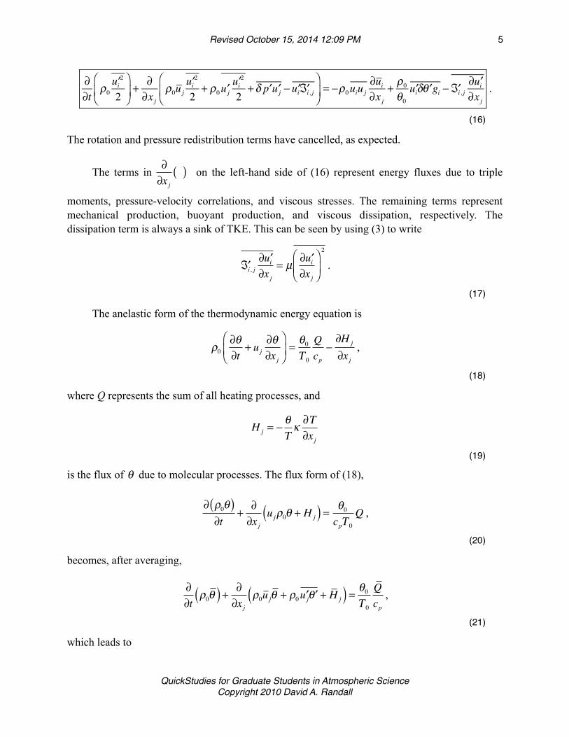
The rotation and pressure redistribution terms have cancelled, as expected.

The terms in ∂∂x j

( ) on the left-hand side of (16) represent energy fluxes due to triple

moments, pressure-velocity correlations, and viscous stresses. The remaining terms represent mechanical production, buoyant production, and viscous dissipation, respectively. The dissipation term is always a sink of TKE. This can be seen by using (3) to write

′ℑi, j∂ ′ui∂x j

= µ ∂ ′ui∂x j

⎛

⎝⎜⎞

⎠⎟

2

.

(17)

The anelastic form of the thermodynamic energy equation is

ρ0∂θ∂t

+ uj∂θ∂x j

⎛

⎝⎜⎞

⎠⎟=θ0Τ 0

Qcp

−∂H j

∂x j,

(18)

where Q represents the sum of all heating processes, and

H j = −θΤκ ∂Τ∂x j

(19)

is the flux of θ due to molecular processes. The flux form of (18),

∂ ρ0θ( )∂t

+∂∂x j

u jρ0θ + H j( ) = θ0cpΤ 0

Q ,

(20)

becomes, after averaging,

∂∂t

ρ0θ( ) + ∂∂x j

ρ0ujθ + ρ0 ′uj ′θ + H j( ) = θ0Τ 0

Qcp

,

(21)

which leads to



ρ0∂θ∂t

+ uj∂θ∂x j

⎛

⎝⎜⎞

⎠⎟= −

∂∂x j

ρ0 ′uj ′θ( ) + θ0Τ 0

Qcp

−∂H j

∂x j.

(22)

Subtraction of (22) from (18) gives

ρ0∂ ′θ∂t

+ uj∂ ′θ∂x j

+ ′uj∂θ∂x j

+ ′uj∂ ′θ∂x j

⎛

⎝⎜⎞

⎠⎟= − ∂

∂x jρ0 ′uj ′θ( ) + θ0

Τ 0

′Qcp

−∂ ′H j

∂x j,

(23)

and multiplication by ′ui then yields

ρ0 ui′∂ ′θ∂t

+ ui′uj∂ ′θ∂x j

+ ui′uj′ ∂θ∂x j

+ ui′uj′ ∂ ′θ∂x j

⎛

⎝⎜⎞

⎠⎟= ui′

∂∂x j

ρ0 ′uj ′θ( ) + θ0Τ 0

ui′ ′Qcp

− ui′∂ ′H j

∂x j.

(24)

Multiplying (12) by ρ0 ′θ , adding the result to (24), averaging, and combining terms, we obtain a

prognostic equation for the potential temperature flux, ρ0 ′ui ′θ :

∂∂t

ρ0ui′ ′θ⎛⎝

⎞⎠ +

∂∂x j

u jρ0ui′ ′θ + uj′ρ0ui′ ′θ⎛

⎝⎞⎠

= −ρ0ui′uj′ ∂θ∂x j

− ρ0uj′ ′θ ∂ui

∂x j+ 2ε i, j ,kρ0uj

′ ′θ Ωk

−ρ0 ′θ ∂∂x j

δ ′pρ0

⎛⎝⎜

⎞⎠⎟+ ρ0

′θ( )2θ0

gi + ′θ∂ ′ℑi, j

∂x j+ θ0Τ 0

ui′ ′Qcp

− ui′∂ ′H j

∂x j(25)

Again, a “triple correlation” has appeared. The heat flux components predicted by (25) can be used in (14), (15), (16), and (22).

Notice that (25) contains ′θ( )2 , which can also be predicted, using

∂∂t

12ρ0 ′θ( )2⎡

⎣⎢⎤⎦⎥+ ∂∂x j

u j12ρ0 ′θ( )2 + uj

′ 12ρ0 ′θ( )2 + ′H j ′θ

⎡

⎣⎢

⎤

⎦⎥ = −ρ0uj

′ ′θ ∂θ∂x j

+ θ0Τ 0

θ ′ ′Qcp

− ′H j∂ ′θ∂x j

.

(26)

Again we see a triple correlation.



In order to complete the second moment equations, we must consider any scalar constituents of the air that are of sufficient interest to warrant prediction. The most important example, and the only one that we will actually consider, is water in its three phases. A parallel discussion can be given for other chemical constituents, e.g., pollutants.

The average conservation equation for total water substance qt is

∂∂t

ρ0qt( ) + ∂∂x j

ρ0uj qt + ρ0uj′qt ′ +Wj

⎛⎝

⎞⎠ = Sw ,

(27)

where Sw represents any possible source (or sink) of qt (e.g., convergence of precipitation flux),

and

Wj = −κ ∂w∂x j

(28)

is the flux of qt due to molecular diffusion. Here we have assumed for simplicity that the

molecular diffusion coefficient for water vapor is the same as that for temperature.

By analogy with (25), we find that

∂∂t

ρ0ui′qt ′⎛⎝

⎞⎠ +

∂∂x j

u jρ0ui′qt ′ + uj′ρ0ui′qt ′

⎛⎝

⎞⎠ = −ρ0ui′uj

′ ∂qt∂x j

− ρ0uj′qt ′

∂u∂x j

+ 2ε i, j ,kρ0uj′qt ′Ωk

−ρ0qt ′∂∂x j

δ ′pρ0

⎛⎝⎜

⎞⎠⎟+ ρ0

qt ′ ′θθ0

gi + qt ′∂ ′ℑi, j

∂x j+ ui′ ′Sw − ui′

∂ ′Wj

∂x j.

(29)

The buoyancy term of (29) is proportional to the covariance of qt and θ , which can be predicted

according to

∂∂t

ρ0qt ′ ′θ⎛⎝

⎞⎠ +

∂∂x j

u jρ0qt ′ ′θ + uj′ρ0qt ′ ′θ⎛

⎝⎞⎠

= −ρ0uj′ ′θ ∂qt

∂x j− ρ0uj

′qt ′∂θ∂x j

+ θ0cpΤ 0

qt ′ ′Q +θ ′ ′Sw − qt ′∂ ′H j

∂x j−θ ′

∂ ′Wj

∂x j.

(30)



We can also derive a prediction equation for qt ′( )2 . Although this quantity does not appear in

any of our other equations, it may be useful to know for other purposes. We include the equation for completeness:

∂∂t

12ρ0 qt ′( )2⎡

⎣⎢

⎤

⎦⎥ +

∂∂x j

u j12ρ0 qt ′( )2 + uj

′ 12ρ0 qt ′( )2 + qt ′ ′Wj

⎡

⎣⎢

⎤

⎦⎥ = −ρ0uj

′qt ′∂qt∂x j

+ qt ′ ′Sw + ′Wj∂qt ′∂x j

.

(31)

Summary

For convenience, we summarize our results in Tables 16.1- 2.

Quantity Equation

Mean momentum

∂ui∂t

+1ρ0

∂∂x j

ρ0uiu j + ρ0 ′ui ′uj − ℑi, j( ) − 2εi, j ,ku jΩk

= −∂∂xi

δ pρ0

⎛

⎝⎜⎞

⎠⎟+δθθ0gi

Mean continuity∂∂xi

ρ0ui( ) = 0

Mean potential temperature∂∂t

ρ0θ( ) + ∂∂x j

ρ0ujθ + ρ0 ′uj ′θ + H j( ) = θ0cpΤ 0

Q

Mean moisture∂∂t

ρ0qt( ) + ∂∂x j

ρ0uj qt + ρ0 ′ujqt ′ +Wj⎛⎝

⎞⎠ = Sw

Table 16.1: The equations for the mean flow.



Quantity Equation

Reynolds stress

∂∂t

ρ0′ui ′u i

2⎛

⎝⎜⎞

⎠⎟+

∂∂x j

ρ0uj′ui ′ui2

+ p0 ′uj12

′ui ′ui − ′ℑi, j ′ui⎛

⎝⎜⎞

⎠⎟+

∂∂xi

δ ′p ′ui( )

= 2εi, j ,kΩkρ0 ′ui ′uj +δ ′pρ0

∂∂xi

ρ0 ′ui( )

+ρ0θ0

′uiδ ′θ gi( ) − ρ0 ′ui ′uj∂ui∂x j

− ′ℑi, j∂ ′ui∂x j

TKE equation

∂∂t

ρ0′ui2

2⎛

⎝⎜

⎞

⎠⎟ +

∂∂x j

ρ0uj′ui2

2+ p0 ′uj

′ui2

2+ δ ′p ′uj( ) − ′u ′ℑi, ji

⎛

⎝⎜

⎞

⎠⎟ =

−ρ0 ′ui ′uj∂ui∂x j

+ρ0θ0

′uiδ ′θ gi − ′ℑi, j∂ ′ui∂x j

Potential temperature flux

∂∂t

ρ0 ′ui ′θ( ) + ∂∂x j

u jρ0 ′ui ′θ + ′ujρ0 ′ui ′θ( )

= −ρ0 ′ui ′uj∂θ∂x j

− ρ0 ′uj ′θ∂ui∂x j

+ 2εi, j ,kρ0 ′uj ′θ Ωk

−ρ0 ′θ∂∂xi

δ ′pρ0

⎛⎝⎜

⎞⎠⎟+ ρ0

′θ( )2θ0

gi + ′θ∂ ′ℑi, j

∂x j+θ0Τ 0

′ui ′Qcp

− ′ui∂ ′H j

∂x j

Potential temperature variance

∂∂t

12ρ0 ′θ( )2⎡

⎣⎢⎤⎦⎥+

∂∂x j

u j12ρ0 ′θ( )2 + ′uj

12ρ0 ′θ( )2 + ′H j ′θ

⎡

⎣⎢

⎤

⎦⎥

= −ρ0 ′uj ′θ∂θ∂x j

+θ0cpΤ 0

′θ ′Q + ′H j∂ ′θ∂x j

Moisture flux

∂∂t

ρ0ui′qt ′⎛⎝

⎞⎠ +

∂∂x j

u jρ0ui′qt ′ + uj′ρ0ui′qt ′

⎛⎝

⎞⎠

= −ρ0ui′uj′ ∂qt∂x j

− ρ0uj′qt ′

∂u∂x j

+ 2ε i, j ,kρ0uj′qt ′Ωk

−ρ0qt ′∂∂x j

δ ′pρ0

⎛⎝⎜

⎞⎠⎟+ ρ0

qt ′ ′θθ0

gi + qt ′∂ ′ℑi, j

∂x j+ ui′ ′Sw − ui′

∂ ′Wj

∂x j.



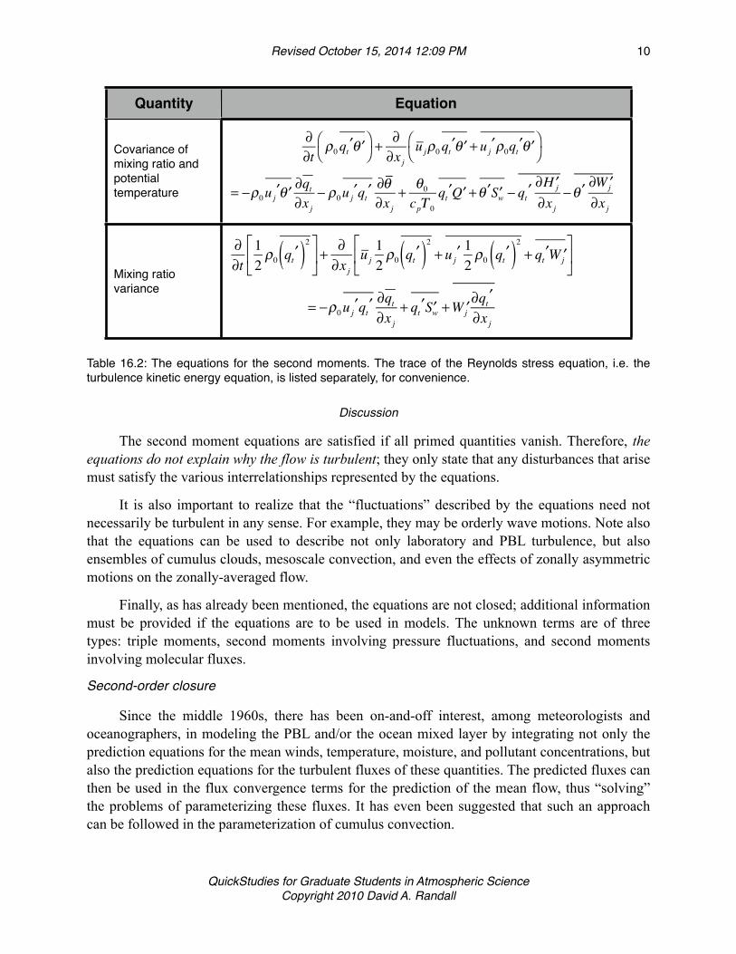
Quantity Equation

Covariance of mixing ratio and potential temperature

∂∂t

ρ0qt ′ ′θ⎛⎝

⎞⎠ +

∂∂x j

u jρ0qt ′ ′θ + uj′ρ0qt ′ ′θ⎛

⎝⎞⎠

= −ρ0uj′ ′θ ∂qt

∂x j− ρ0uj

′qt ′∂θ∂x j

+ θ0cpΤ 0

qt ′ ′Q +θ ′ ′Sw − qt ′∂ ′H j

∂x j−θ ′

∂ ′Wj

∂x j

Mixing ratio variance

∂∂t

12ρ0 qt ′( )2⎡

⎣⎢

⎤

⎦⎥ +

∂∂x j

u j12ρ0 qt ′( )2 + uj

′ 12ρ0 qt ′( )2 + qt ′ ′Wj

⎡

⎣⎢

⎤

⎦⎥

= −ρ0uj′qt ′

∂qt∂x j

+ qt ′ ′Sw + ′Wj∂qt ′∂x j

Table 16.2: The equations for the second moments. The trace of the Reynolds stress equation, i.e. the turbulence kinetic energy equation, is listed separately, for convenience.

Discussion

The second moment equations are satisfied if all primed quantities vanish. Therefore, the equations do not explain why the flow is turbulent; they only state that any disturbances that arise must satisfy the various interrelationships represented by the equations.

It is also important to realize that the “fluctuations” described by the equations need not necessarily be turbulent in any sense. For example, they may be orderly wave motions. Note also that the equations can be used to describe not only laboratory and PBL turbulence, but also ensembles of cumulus clouds, mesoscale convection, and even the effects of zonally asymmetric motions on the zonally-averaged flow.

Finally, as has already been mentioned, the equations are not closed; additional information must be provided if the equations are to be used in models. The unknown terms are of three types: triple moments, second moments involving pressure fluctuations, and second moments involving molecular fluxes.

Second-order closure

Since the middle 1960s, there has been on-and-off interest, among meteorologists and oceanographers, in modeling the PBL and/or the ocean mixed layer by integrating not only the prediction equations for the mean winds, temperature, moisture, and pollutant concentrations, but also the prediction equations for the turbulent fluxes of these quantities. The predicted fluxes can then be used in the flux convergence terms for the prediction of the mean flow, thus “solving” the problems of parameterizing these fluxes. It has even been suggested that such an approach can be followed in the parameterization of cumulus convection.



As noted above, the problem with this approach is that the second-moment equations involve unknown quantities. Chief among these are all “triple moment” terms, but all terms involving pressure perturbations and all terms involving molecular diffusion are also unknown. These terms have to be “modeled” or “parameterized,” in terms of known quantities.

Donaldson (1973) gave a very readable introduction to the use of the prediction equations for the second moments. He listed four principles that, he argues, should be applied in devising parameterizations of terms of the second-moment equations

1) The parameterization must be invariant under an arbitrary transformation of coordinate systems. The parameterization must therefore have all the tensor properties and, in addition, all the symmetries of the term that it replaces.

2) The parameterization must be invariant under a Galilean transformation, i.e. if we shift to a second coordinate system that is in constant motion relative to the first, the equations are unchanged.

3) The parameterization must have the dimensional properties of the term it re-places.

4) The parameterization must satisfy all the conservation relationships known to govern the variables in question.

All authors mentioned here use the “tendency-towards-isotropy” model of the pressure-shear covariance terms of the Reynolds stress equation, i.e.

∂∂t

ρ0 ′ui ′ul( ) ~ δ ′pρ0

∂∂xi

ρ0 ′ul( ) + ∂∂xl

ρ0 ′ui( )⎡

⎣⎢

⎤

⎦⎥ =

−q3l1

′ui ′ul −δ il3q2⎛

⎝⎜⎞⎠⎟

,

(32)

where

q2 ≡ ′uk ′uk≡ 2e ,

(33)

and l1 is a length scale that has to be prescribed. If the turbulence is truly isotropic, then only the

diagonal members of ′ui ′ul are non-zero (because the others are fluxes), and these three diagonal

members must each be equal to 13q2 , so that ′ui ′ul −

δ il3q2 , which appears on the right-hand-side

of (32), will vanish. The term is thus formulated as a measure of the departure from isotropy.

Notice that if ′ui ′ul departs from its isotropic value (0 for the off-diagonal members, and 13q2 for



the diagonal members), then the term will tend to force it back towards isotropy. One effect of this is that the Reynolds stresses can’t become too large. This model of the term stems from the recognition that the pressure-shear covariance terms only redistribute kinetic energy among the three components. It was first suggested by Rotta (1951).

In a similar way, we take

′p∂ ′θ∂xi

= −q3l2

′ui ′θ( ) ,

(34)

and

′p∂ ′w∂xi

= −q3l3

′ui ′w( ) ,

(35)

in the prediction equations for ρ0 ′ui ′θ and ρ0 ′ui ′w respectively.

The remaining terms of these equations that involve ′p are all derivatives, and so should

tend to vanish when integrated over sufficiently large regions. They are therefore modelled as transport terms.

′p ′uk ~ −ρ0λ1q∂∂xi

′ui ′uk( ) ,

(36)

′p ′θ ~ −ρ0λ1q∂∂xi

′ui ′θ( ) ,

(37)

′p ′w ~ −ρ0λ1q∂∂xi

′ui ′w( ) .

(38)

The “triple correlation” terms of the forecast equations are also transport terms. The total model is then

− ∂∂x j

ρ0 ′ui ′uj ′ul( ) − ∂∂xi

′ul ′p( ) − ∂∂xl

′ui ′p( ) = ∂∂xk

qλ1∂∂xk

ρ0 ′ui ′ul( ) + ∂∂xi

ρ0 ′ul ′uk( ) + ∂∂xl

ρ0 ′uk ′ui( )⎡

⎣⎢

⎤

⎦⎥

⎧⎨⎪

⎩⎪

⎫⎬⎪

⎭⎪,

(39)



−∂∂x j

′ujρ0 ′ui ′w( ) − ρ0∂∂xi

′p ′wρ0

⎛

⎝⎜⎞

⎠⎟=

∂∂xk

qλ4∂∂xk

ρ0 ′ui ′w( ) + ∂∂xi

ρ0 ′ui ′w( )⎡

⎣⎢

⎤

⎦⎥

⎧⎨⎪

⎩⎪

⎫⎬⎪

⎭⎪.

(40)

Similarly, the triple correlation terms of the scalar variance and covariance forecast equations are modelled as down-gradient diffusion terms:

−∂∂x j

′uj12ρ0 ′θ( )2⎛

⎝⎜⎞

⎠⎟=

∂∂xk

qλ2∂∂xk

12ρ0 ′θ( )2⎡

⎣⎢⎤⎦⎥

⎧⎨⎩

⎫⎬⎭

,

(41)

−∂∂x j

′ujρ0 ′w ′θ( ) = ∂∂xk

qλ5∂∂xk

ρ0 ′w ′θ( )⎡

⎣⎢

⎤

⎦⎥ ,

(42)

−∂∂x j

′uj12ρ0 ′w( )2⎛

⎝⎜⎞

⎠⎟=

∂∂xk

qλ6∂∂xk

12ρ0 ′w( )2⎡

⎣⎢⎤⎦⎥

⎧⎨⎩

⎫⎬⎭

.

(43)

All of these assumptions are “safe;” the modelled terms will not blow up in a computer simulation. None of the assumptions is very convincing -- no more convincing than the mixing length theory that they replace. There is what Lumley calls an “article of faith,” that weak assumptions at third order are preferable to weak assumptions at second order. As discussed later, the results are rather convincing.

The dissipation terms of the variance production equations are modelled as exponential decay, while all other molecular terms are neglected:

−′ℑi, j

ρ0

∂ ′ul∂x j

−′ℑl , j

ρ0

∂ ′ui∂x j

= −23q3

Λ1δ il ,

(44)

∂∂x j

′ul ′ℑi, j + ′ui ′ℑl , j( ) = 0 ,

(45)

′θ∂ ′ℑi, j

∂x j− ′ui

∂ ′H j

∂x j= 0 ,

(46)



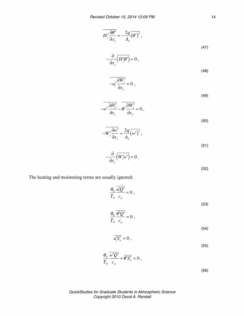
′H j∂ ′θ∂x j

= − 2qΛ2

′θ( )2 ,

(47)

−∂∂x j

′H j ′θ( ) = 0 ,

(48)

− ′ui∂ ′Wj

∂x j= 0 ,

(49)

− ′w∂ ′H j

∂x j− ′θ

∂ ′Wj

∂x j= 0 ,

(50)

− ′Wj∂ ′w∂x j

=2qΛ3

′w( )2 ,

(51)

−∂∂x j

′Wj ′w( ) = 0 .

(52)

The heating and moistening terms are usually ignored:

θ0Τ 0

′ui ′Qcp

= 0 ,

(53)

θ0Τ 0

′θ ′Qcp

= 0 ,

(54)

′ui ′Sw = 0 ,(55)

θ0Τ 0

′w ′Qcp

+ ′θ ′Sw = 0 ,

(56)



′w ′Sw = 0 .(57)

No one argues that they are negligible in all cases, although no doubt they are in some. Their potential importance must be faced where the equations are applied to clouds.

In most theories, all of the various length scales introduced above are assumed to be proportional to each other, and the proportionality factors are assumed to be constants. The models are “tuned” by choice of these constants. Usually no attempt is made to argue that the constants are “universal,” although it is openly (but tacitly) assumed that they are.

A variety of different closure theories can be constructed by choice of retained terms in the equations. We now survey a few of these theories.

Mellor and Yamada (1974) presented a hierarchy of turbulence closure models, ranging form a fully prognostic system of second-moment equations (Level 4) to a fully diagnostic subset corresponding to mixing length theory (Level 1). These are summarized in Table 16.3.

Level Prognostic variables

4 Reynolds stress tensor (six equations)

′θ( )2 (one equation)

Heat flux vector (three equations)

3 Turbulence kinetic energy (one equation)

′θ( )2 (one equation)

2 None

1 None

Table 16.3: Prognostic variables of the dry Mellor-Yamada models.

None of the models includes molecular effects other than dissipation, or diabatic effects, or coriolis effects (except in the equation of mean motion), or buoyant production of momentum, heat, and moisture fluxes. All of the models are Boussinesq (up to now we have used the anelastic system). Level 4 then includes 15 differential equations for the second moments, in addition to 5 for the mean flow. Of course, modeling of pollutant transport would require additional equations. At Level 3, only three differential equations are used for the second

moments - those for e, ′θ( )2 , and ′w( )2 . Levels 2 and 1 involve only diagnostic relations for all

of the second moments. Level 1 turns out to be equivalent to the “mixing length” theory.



Mellor and Yamada experimented with each of the models, and concluded that in most applications the additional realism obtained at Level 4 was not sufficiently better than that at Level 3 to warrant the additional computational complexity. Of course, this conclusion is based in part on the parameterizations that they used for the triple moments, the dissipation terms, and the pressure terms.

Wyngaard and Coté (1974) and Wyngaard (1975) applied a simplified version of the Lumley-Khajeh-Nouri model to the simulation of both the unstable and the stable PBLs, comparing their results to the Wangara and Minnesota observations, and to the more detailed calculations of Deardorff.

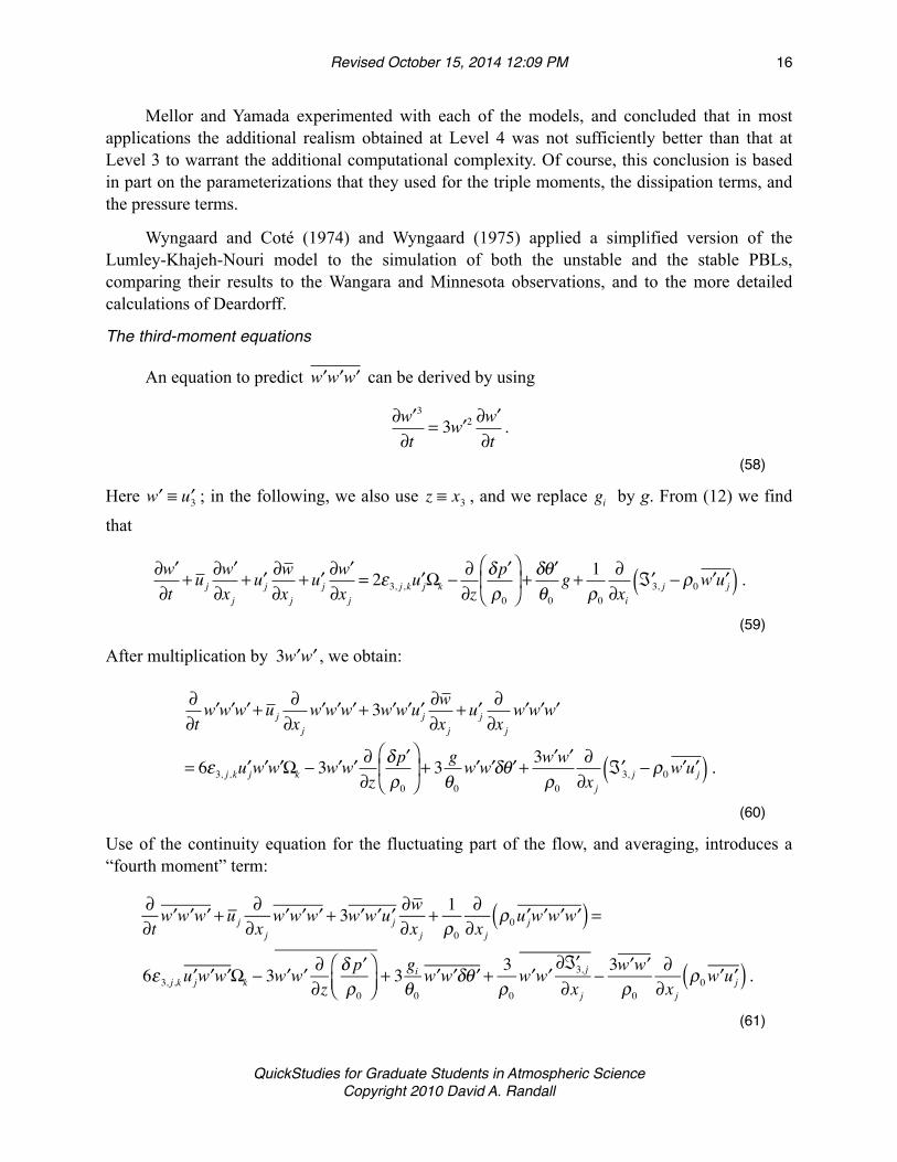
The third-moment equations

An equation to predict ′w ′w ′w can be derived by using

∂ ′w 3

∂t= 3 ′w 2 ∂ ′w

∂t.

(58)

Here ′w ≡ ′u3 ; in the following, we also use z ≡ x3 , and we replace gi by g. From (12) we find

that

∂ ′w∂t

+ uj∂ ′w∂x j

+ ′uj∂w∂x j

+ ′uj∂ ′w∂x j

= 2ε3, j ,k ′ujΩk −∂∂z

δ ′pρ0

⎛

⎝⎜

⎞

⎠⎟+

δ ′θθ0

g + 1ρ0

∂∂xi

′ℑ3, j − ρ0 ′w ′uj( ) .

(59)

After multiplication by 3 ′w ′w , we obtain:

∂∂t

′w ′w ′w + uj∂∂x j

′w ′w ′w + 3 ′w ′w ′uj∂w∂x j

+ ′uj∂∂x j

′w ′w ′w

= 6ε3, j ,k ′uj ′w ′wΩk − 3 ′w ′w ∂∂z

δ ′pρ0

⎛

⎝⎜

⎞

⎠⎟+ 3

gθ0

′w ′wδ ′θ + 3 ′w ′wρ0

∂∂x j

′ℑ3, j − ρ0 ′w ′uj( ) .(60)

Use of the continuity equation for the fluctuating part of the flow, and averaging, introduces a “fourth moment” term:

∂∂t

′w ′w ′w + uj∂∂x j

′w ′w ′w + 3 ′w ′w ′uj∂w∂x j

+ 1ρ0

∂∂x j

ρ0 ′uj ′w ′w ′w( ) =

6ε3, j ,k ′uj ′w ′w Ωk − 3 ′w ′w ∂∂z

δ ′pρ0

⎛⎝⎜

⎞⎠⎟+ 3 gi

θ0′w ′w δ ′θ + 3

ρ0′w ′w

∂ ′ℑ3, j

∂x j− 3 ′w ′w

ρ0∂∂x j

ρ0 ′w ′uj( ) .(61)



Normally (61) is simplified by neglecting advection by the mean flow, the production term

involving ∂w∂x j

, the rotation term, and 3 ′w ′wρ0

∂∂x j

ρ0 ′w ′uj( ) :

∂∂t

′w ′w ′w + 1ρ0

∂∂x j

ρ0 ′uj ′w ′w ′w( ) = −3 ′w ′w ∂∂z

δ ′pρ0

⎛⎝⎜

⎞⎠⎟+ 3 gi

θ0′w ′w δ ′θ + 3

ρ0′w ′w

∂ ′ℑ3, j

∂x j.

(62)

An equation to predict ′θ ′θ ′θ can be written down by mimicking (61), with reference to (23):

∂∂t

′θ ′θ ′θ + uj∂∂x j

′θ ′θ ′θ + 3 ′w ′w ′uj∂θ∂x j

+ 1ρ0

∂∂x j

ρ0 ′uj ′θ ′θ ′θ( ) = 3ρ0

′θ ′θ∂ ′H j

∂x j− 3 ′θ ′θ

ρ0∂∂x j

ρ0 ′uj ′θ( )(63)

Third- order closure

André and collaborators (1976 a, b, 1978) constructed a model in which the third moments are predicted, and the fourth moments are expanded in terms of the second moments through the quasi-normal approximation:

′a ′b ′c ′d ≅ ′a ′b ′c ′d + ′a ′c ′b ′d + ′a ′d ′b ′c ,(64)

which is exact if a, b, c and d are Gaussian random variables. It has been shown that models based on this idea predict the development of negative variances, and other non-physical behavior. André et al. suggested that the difficulty can be avoided by requiring that the third moments satisfy Schwartz’s inequality, which can be expressed as

′a ′b ′c ≤ min

a2 b2 ′c 2 + ′b ′c( )2⎡⎣⎢

⎤⎦⎥

⎧⎨⎩

⎫⎬⎭

1/2

b2 a2 ′c 2 + ′a ′c( )2⎡⎣⎢

⎤⎦⎥

⎧⎨⎩

⎫⎬⎭

1/2

c2 a2 ′b 2 + ′a ′b( )2⎡⎣⎢

⎤⎦⎥

⎧⎨⎩

⎫⎬⎭

1/2

⎧

⎨

⎪⎪⎪⎪

⎩

⎪⎪⎪⎪

⎫

⎬

⎪⎪⎪⎪

⎭

⎪⎪⎪⎪

.

(65)

This is called a “realizability” constraint.

Third-moment closure is being used in some high-resolution cloud models (e.g. Krueger 1988).



References and BibliographyAndré, J. C., G. DeMoor, P. Lacarre're, and R. du Vachat, 1976: Turbulence approximation for

inhomogeneous flows. Part I: The clipping approximation. J. Atmos. Sci., 33, 476-481.

André, J. C., G. DeMoor, P. Lacarre're, and R. du Vachat, 1976: Turbulence approximation for inhomogeneous flows. Part II: The numerical simulation of a penetrative convection ex-periment. J. Atmos. Sci., 33, 482-491.

André, J. C., G. DeMoor, P. Lacarre're, G. Therry, and R. Du Vachat, 1978: Modeling the 24-hour evolution of the mean and turbulent structures of the planetary boundary layer. J. Atmos. Sci., 35, 1861-1883.

Andren, A., and C.-H. Moeng, 1993: Single-point closures in a neutrally stratified boundary layer. J. Atmos. Sci., 50, 3365-3379.

Bougeault, Ph., 1981: Modeling the trade-wind cumulus boundary layer. Part I: Testing the en-semble cloud relations against numerical data. J. Atmos. Sci., 38, 2414-2428.

Bougeault, Ph., 1981: Modeling the trade-wind cumulus boundary layer. Part II: A high order one dimensional model. J. Atmos. Sci., 38, 2429-2439.

Bougeault, Ph., 1982: Cloud-ensemble relations based on the Gamma probability distribution for the higher-order models of the planetary boundary layer. J. Atmos. Sci., 39, 2691-2700.

Bougeault, Ph., 1985: The diurnal cycle of the marine stratocumulus layer: A higher-order model study. J. Atmos. Sci., 42, 2826-2843.

Bougeault, P., and J.-C. André, 1986: On the stability of the third-order turbulence closure for the modeling of the stratocumulus boundary layer. J. Atmos. Sci., 43, 1574-1581.

Burchard, H., and H. Baumert, 1995: On the performance of a mixed-layer model based on the k-e turbulence closure. J. Geophys. Res., 100, 8523-8540.

Canuto, V. M., F. Minotti, C. Ronchi, R. M. Ypma, and O. Zeman, 1994: Second-order closure PBL model with new third-order moments: Comparison with LES data. J. Atmos. Sci., 51, 1605-1618.

Canuto, V. M., and Y. Cheng, 1994: Stably stratified shear turbulence: A new model for the en-ergy dissipation length scale. J. Atmos. Sci., 51, 2384-1618.

Chen, C., and W. R. Cotton, 1983: A one-dimensional simulation of the stratocumulus-capped mixed layer. Bound.-Layer Meteor., 25, 289-322.

Chen, J.-M., 1991: Turbulence-scale condensation parameterization. J. Atmos. Sci., 48, 1510--1512. (contains numerous typographical errors)



Deardorff, J. W., 1978: Closure of second- and third-moment rate equations for diffusion in ho-mogeneous turbulence. Phys. Fluids, 21, 525-530.

Deardorff, J. W., and G. Sommeria, 1977: Subgrid-scale condensation in models of nonprecipi-tating clouds. J. Atmos. Sci., 34, 344-355.

Deardorff, J. W., and L. Mahrt, 1983: On the dichotomy in theoretical treatments of the atmos-pheric boundary layer. J. Atmos. Sci., 39, 2096-2098.

Donaldson, C., 1973: Construction of a dynamic model of the production of atmospheric turbu-lence and the dispersal of atmospheric pollutants. Workshop on Micrometeorology, D. A. Haugen, ed., Amer. Meteorol. Soc., Boston, 313-392.

Finger, J. E., and H. Schmidt, 1986: On the efficiency of different higher order turbulence mod-els simulating the convective boundary layer. Beitr. Phys. Atmos., 59, 505-517.

Janjic, Z. I., 1990: The step-mountain coordinate: Physical package. Mon. Wea. Rev., 118, 1429-1443.

Krueger, S. K., 1985: Numerical simulation of tropical cumulus clouds and their interaction with the subcloud layer. Ph.D. Dissertation, Dept. of Atmospheric Sciences, UCLA, 205 p.

Krueger, S. K., 1988: Numerical simulation of tropical cumulus clouds and their interaction with the subcloud layer. J. Atmos. Sci., 45, 2221-2250.

Launder, B. E., 1975: On the effects of a gravitational field on the turbulent transport of heat and momentum. J. Fluid. Mech., 67, 569-581.

Launder, B.E., Reece, G.J. & Rodi, W. 1975: Progress in the development of a Reynolds-stress turbulence closure. J. Fluid Mech. 68, 537-566.

Leonard, A., 1974: Energy cascade in large-eddy simulations of turbulent fluid flows. Adv. Geo-phys., A18, 237-248.

Lenschow, D. H., J. C. Wyngaard, and W. T. Pennell, 1980: Mean-field and second-moment budgets in a baroclinic, convective boundary layer. J. Atmos. Sci., 37, 1313-1326.

Lewellen, W. S., and M. E. Teske, 1973: Prediction of the Monin-Obukhov similarity functions from an invariant model of turbulence. J. Atmos. Sci., 30, 1340-1345.

Lewellen, W. S., 1977: Use of invariant modeling. In Handbook of Turbulence, W. Frost and T. H. Moulden, Eds., Plenum, 237-280.

Lewellen, W. S., and S. Yoh, 1993: Binormal model of ensemble cloudiness. J. Atmos. Sci., 50, 1228-1237.

Lilly, D. K., 1992: A proposed modification of the Germano subgrid-scale closure method. Phys. Fluids A, 4, 633-635.



Lumley, J. L., 1978: Computational modeling of turbulent flows. Adv. Appl. Mech., 18, 123-176.

Lumley, J.L., O. Zeman, and J. Seiss, 1978: The influence of buoyancy on turbulent transport. J. Fluid Mech., 84, 581-597.

Mellor, G. L., 1973: Analytic prediction of the properties of stratified planetary surface layers. J. Atmos. Sci., 30, 1061-1069.

Mellor, G. L., 1977: The Gaussian cloud model relations. J. Atmos. Sci., 34, 356-358.

Mellor, G. L., and T. Yamada, 1974: A hierarchy of turbulence closure models for the planetary boundary layer. J. Atmos. Sci., 31, 1791-1806.

Mellor, G. L., and T. Yamada, 1982: Development of a turbulence closure model for geophysical fluid problems. Rev. Geophys. Space Phys., 20, 851-875.

Moeng, C.-H., and D. A. Randall, 1984: Problems in simulating the stratocumulus-topped boundary layer with a third-order closure model. J. Atmos. Sci., 41, 1588-1600.

Moeng, C.-H., and J. C. Wyngaard, 1986: An analysis of closures for pressure-scalar covariances in the convective boundary layer. J. Atmos. Sci., 43, 2499-2513.

Moeng, C.-H., and J. C. Wyngaard, 1989: Evaluation of turbulent transport and dissipation clo-sures in second-order modeling. J. Atmos. Sci., 46, 2311--2330.

Monin, A. S., and A. M. Yaglom, 1971: Statistical fluid mechanics. Vol. 1. Mechanics of turbu-lence. MIT Press, Cambridge, Mass., 769 pp.

Oliver, D. A., W. S. Lewellen, and G. G. Williamson, 1978: The interaction between turbulent and radiative transport in the development of fog and low-level stratus. J. Atmos. Sci., 35, 301-316.

Randall, D. A., 1987: Turbulent fluxes of liquid water and buoyancy in partly cloudy layers. J. Atmos. Sci., 44, 850-858.

Randall, D. A., Q. Shao, and C.-H. Moeng 1992: A second-order bulk boundary-layer model. J. Atmos. Sci., 49, 1903-1923.

Smagorinski, J., 1963: General circulation experiments with the primitive equations. Mon. Wea. Rev., 91, 99-164.

Wyngaard, J. C., 1980: The atmospheric boundary layer - Modeling and measurements. In Tur-bulent Shear Flows 2, J. S. Bradbury, ed., Springer-Verlag, Berlin, pp. 352-365.

Wyngaard, J. C., 1982: Boundary layer modeling. In Atmospheric Turbulence and Air Pollution Modeling, F. T. M. Nieuwstadt and H. Van Dop, Eds., Reidel, 69-106.



Wyngaard, J. C., and O. R. Cote', 1971: The budgets of turbulent kinetic energy and temperature variance in the atmospheric surface layer. J. Atmos. Sci., 28, 190-201.

Wyngaard, J. C., and O. R. Cote', 1974: Evolution of a convective planetary boundary layer - A higher-order closure model study. Bound.-Layer Meteor., 7, 289-304.

Wyngaard, J. C., W. T. Pennell, D. H. Lenschow, and M. A. LeMone, 1978: The temperature-humidity covariance budget in the convective boundary layer. J. Atmos. Sci., 35, 47-58.

Yamada, T., and C.-Y. J. Kao, 1986: A modeling study on the fair weather marine boundary layer of the GATE. J. Atmos. Sci., 43, 3186-3199.

Yamada, T., and G. L. Mellor, 1975: A simulation of the Wangara atmospheric boundary layer data. J. Atmos. Sci., 32, 2309-2329.

Yamada, T., and G. L. Mellor, 1979: A numerical simulation of BOMEX data using a turbulence closure model coupled with ensemble cloud relations. Quart. J. Roy. Meteor. Soc., 105, 915-944.

Zeman, O., 1979: Parameterization of the dynamics of stable boundary layer flow and nocturnal jets. J. Atmos. Sci., 30, 792-804.

Zeman, O., and J. L. Lumley, 1976: Modeling buoyancy-driven mixed layers. J. Atmos. Sci., 33, 1974-1988.

Zeman, O., and H. Tennekes, 1977: Parameterization of the turbulent energy budget at the top of the daytime atmospheric boundary layer. J. Atmos. Sci., 34, 111-123.

Zeman, O., 1981: Progress in the modeling of planetary boundary layers. Ann. Rev. Fluid Mech., 13, 253-272.



First- and Second-Moment...

Documents

Transcript of First- and Second-Moment...