Firm vs. Bank Leverage over the Business...

Firm vs. Bank Leverage over the Business Cycle

Rohan Kekre∗

May 13, 2016

Abstract

I develop a general equilibrium model with asymmetric information between issuers and

investors to explain the contrasting cyclical behavior of leverage for non-financial corporates

(“firms”) and financial intermediaries (“banks”) in U.S. data. Firm leverage is countercyclical

because the lemons discount in equity issuance falls relative to the costs of financial distress

in a boom. Bank leverage is procyclical because banks are endogenously more diversified than

firms and their capacity to issue safe debt, the cheapest form of external finance, increases in

a boom. The model explains additional cross-sectional differences in leverage cyclicality, such

as between commercial banks and broker/dealers, and between more and less bank-dependent

firms. Normatively, there is a role for macroprudential regulation of the level of bank leverage

but not its cyclicality, as the procyclicality of bank safe debt issuance is constrained efficient.

∗Department of Economics, Harvard University. Email: [email protected]. For invaluable guidance onthis project, I sincerely thank Malcolm Baker, Gabriel Chodorow-Reich, Emmanuel Farhi, Gita Gopinath, RobinGreenwood, Sam Hanson, Victoria Ivashina, Ken Rogoff, David Scharfstein, Andrei Shleifer, Alp Simsek, JeremyStein, and Adi Sunderam. For many helpful discussions, I also thank Eduardo Davila, Ben Hebert, Divya Kirti,Vijay Narasiman, Vania Stavrakeva, and David Yang.

1

1 Introduction

Since the 2008-09 financial crisis, the capital structure of financial intermediaries has come under

heavy scrutiny in the public and academic debate. Relative to non-financial corporates, intermedi-

ary leverage has been shown to be unique both in its level and its cyclicality over time. As Figure

1 shows using Fed Flow of Funds data, the leverage of broker/dealers has been slightly more than

twice that of corporates over the past thirty years. As Figure 2 shows using cyclical variation in the

same data, the leverage of broker/dealers covaries positively with log real GDP — it is procylical

— while that of corporates is countercyclical.1 As Adrian and Shin [2010a,b, 2011] have empha-

sized in an early series of papers documenting these facts, such procyclicality may be an important

mechanism by which the financial sector exacerbates economic fluctuations.

Why do intermediaries (“banks”) and non-financial corporates (“firms”) manage their leverage

so differently over the business cycle? While there is an established literature on the level of bank

leverage and importance of debt in the liability structure of banks more generally2, the difference in

leverage cyclicality remains a puzzle. In this paper, I provide one theory which can rationalize the

difference in leverage of firms and banks over the business cycle. I use this framework to explain

additional cross-sectional facts in the data. In an evaluation of social welfare, I then speak directly

to current policy debates over macroprudential regulation in banking.

I argue that the endogenous diversification of banks on the asset side of their balance sheet

can rationalize the procylicality of bank leverage and countercyclicality of firm leverage in general

equilibrium. Following Diamond [1984], banks are characterized as delegated monitors who diversify

across their investments so that they may issue safe debt, the cheapest form of external finance in

an environment with asymmetric information and costs of financial distress. In an economic upturn

characterized by an improvement in the underlying distribution of project quality, firms see the

lemons discount in equity issuance fall relative to the cost of financial distress, driving a reduction

in firm leverage. In contrast, as diversified intermediaries, banks facing the same macroeconomic

shock see their capacity to issue safe debt expand, driving an increase in bank leverage.

This perspective on banks and firms can rationalize additional cross-sectional patterns in the

data and, normatively, implies that the procyclicality of leverage is an efficient property of banking.

Within the banking sector, banks with access to deposit insurance exhibit less procyclical lever-

age than other types of banks, and are re-intermediated in downturns, consistent with empirical

evidence comparing commercial banks with broker/dealers. Among firms, bank-dependent firms

exhibit more procyclical leverage than non-bank-dependent firms because the improved funding

conditions for banks are inherited by the former set of firms in general equilibrium, consistent with

empirical evidence on LBO targets and smaller firms. Finally, the issuance of safe debt is an efficient

response to the informational and technological frictions in the economy. As such, recent proposals

1Leverage is computed as Debt/Assets, consistent with its definition in the model which follows. Cyclical variationis computed by running each series through a Hodrick-Prescott filter with smoothing parameter λ = 1600.

2Among other papers, see Diamond and Dybvig [1983], Diamond [1984], Gorton and Pennacchi [1990], Calomirisand Kahn [1991], Flannery [1994], and Diamond and Rajan [2000].

2

Average

1.8

1.9

22

.12

.22

.3

1985q1 1990q1 1995q1 2000q1 2005q1 2010q1 2015q1

Broker/Dealer Leverage / Nonfinancial Corporate Leverage

Construction: leverage = debt / assets

Source: Fed Flow of Funds, 1984Q1-2013Q1

Figure 1: Broker/dealer vs. non-financial corporate leverage: level

-.01

-.00

50

.00

5.0

1B

roker/

De

ale

r Le

ve

rag

e (

cyclic

al)

-.03 -.02 -.01 0 .01 .02Log Real GDP (cyclical)

Cyclical Broker/Dealer Leverage and Log Real GDP

Construction: leverage = debt / assets, and cyclical components obtained using HP filter ( = 1600)

Source: Fed Flow of Funds and Bureau of Economic Analysis, 1984Q1-2013Q1



-.04

-.02

0.0

2.0

4N

on

fin. C

orp

ora

te L

evera

ge

(cyclic

al)


Cyclical Nonfin. Corporate Leverage and Log Real GDP

Figure 2: Broker/dealer vs. non-financial corporate leverage: cyclicality

for countercyclical capital requirements in banking may be misplaced, since the procyclicality of

bank leverage is constrained efficient even if the level of bank leverage is not.

I begin by specifying a general equilibrium environment with three sets of agents — households,

entrepreneurs, and bankers — in which two chains of financing and investment co-exist. In the first

chain, entrepreneurs directly issue bond or equity securities to household investors so that they

may invest in a proprietary, fixed scale investment technology. I interpret these entrepreneurs as

corresponding to the non-financial corporate sector in the U.S., where little financing is obtained

through the banking sector. In the second chain, a distinct set of entrepreneurs can directly issue

bonds to household investors or take out a bank loan from bankers so that they may invest in

their own proprietary, fixed scale investment technology. Bankers, in turn, issue bond or equity

securities to household investors. I interpret these entrepreneurs as corresponding to mortgage

borrowers in the U.S., who ultimately obtain financing through securitization markets or loans

held on balance sheet by the banking sector. In general equilibrium, the expected rates of return

earned by (risk-neutral) household investors across securities must be equalized.

To obtain concrete financing predictions and clarify the role of bankers in the economy, I then

assume three sets of frictions relative to the Modigliani and Miller [1958] benchmark. First, I assume

3

that entrepreneurs have private information regarding the quality of their investment technology.

Second, I assume that through loans to entrepreneurs, bankers can eliminate this informational

asymmetry at an upfront monitoring cost — but, paralleling the assumption for entrepreneurs,

bankers’ monitoring cost is private information. Third, I assume that through bond finance of

either entrepreneurs or bankers, households can eliminate the informational asymmetry but will

incur an ex-post cost of financial distress should the entrepreneur or banker default.

In this environment, firm leverage is countercyclical because the lemons discount in equity

issuance falls relative to the costs of financial distress from bond issuance in a boom. With a

continuum of firms whose investment quality is drawn from a continuous distribution, in equilibrium

firms optimally finance themselves in a manner consistent with intuition of Myers and Majluf

[1984]’s pecking-order: low-quality firms forego investment, medium-quality firms issue equity and

invest, and high-quality firms issue debt and invest. In an economic upturn characterized by an

improvement in the distribution of firm quality, the lemons discount associated with equity issuance

falls for the marginal bond issuer, driving a relative increase in equity issuance vs. bond issuance

in the corporate sector. This mechanism is similar to one proposed by Choe et al. [1993] in their

explanation of procylical seasoned equity offerings over the business cycle.

In contrast to firms, bank leverage is procyclical because banks are endogenously diversified

across idiosyncratic risk and their capacity to issue safe debt, the cheapest form of external finance,

increases in a boom. Consistent with the results in Diamond [1984], bankers lend to a pool of

entrepreneurs and, by tranching debt on the liability side of their balance sheet, issue default-free

debt that is free of asymmetric information and costs of financial distress. The remainder of their

capital structure is pinned down by focusing on an equilibrium in which bankers separate from less

skilled bankers by issuing enough costly, risky bonds, while also being consistent with free entry

into banking. In an economic upturn, the improvement in the quality of entrepreneur projects leads

to an increase in the safe debt capacity of bankers, driving the procyclicality of bank leverage.

From a positive perspective, extensions of this framework can explain additional cross-sectional

patterns in the data. First, the model clarifies why commercial banks may exhibit less procycli-

cal leverage than broker/dealers, a point made by He et al. [2010] and He and Krishnamurthy

[2012].3 Commercial banks are distinguished from these other intermediaries by their participation

in government-provided deposit insurance. In the model, deposit insurance means that banks’ safe

debt capacity need not fall in a downturn, preventing them from needing to delever. Because their

weighted average cost of capital is unchanged, it also means that the interest rate they must charge

on loans need not rise, so their assets do not fall. This is consistent with the reintermediation of

commercial banks discussed in Gatev and Strahan [2006] and Ivashina and Scharfstein [2010].

Second, the model clarifies why bank-dependent firms may exhibit more procyclical leverage

than other firms, consistent with the findings of Axelson et al. [2013] for LBO targets and Leary

[2009] for small firms. Bank-dependent firms can be modeled as a set of entrepreneurs who can

3In particular, these authors argue that commercial bank leverage is countercyclical when measured using marketleverage. As I show in section 5, commercial bank leverage remains procyclical, but is indeed less procyclical thanbroker/dealer leverage, using the marked-to-market book leverage measure obtained using the Fed Flow of Funds.

4

finance themselves using bonds, bank loans, or equity. For such entrepreneurs, a general equilib-

rium effect implied by the model is that the higher safe debt capacity and thus improved funding

conditions for banks translate to a lower interest rate on bank loans in a boom. This force offsets

the lower lemons discount from equity issuance in a boom, and means that their leverage will be

more procylical than that of other firms, holding the initial level of leverage the same.

From a normative perspective, the present framework motivates a role for a binding leverage cap

in banking, but does not justify any use of this cap to offset the procyclicality of bank leverage. The

equilibrium under consideration features excessive risky debt issuance as skilled bankers attempt to

signal their quality to the market. The source of the inefficiency is agents’ coordination at a Pareto

inferior equilibrium among the many possible equilibria arising between entrepreneurs, bankers,

and households, common to signaling models in the tradition of Spence [1973]. In particular, at

a high interest rate on bank loans, skilled bankers have an incentive to separate from unskilled

bankers by issuing costly risky debt, raising their cost of capital and supporting the high interest

rate in equilibrium. A cap on bank leverage prevents skilled bankers from signaling their quality to

the market, and if sufficiently low can break coordination at the ‘high interest rate - high leverage’

equilibrium, generating a utilitarian welfare increase. However, even in the resulting constrained

efficient allocation, bank safe debt capacity is procyclical. In this way, procyclical leverage is an

efficient property of banking, even though its high level of leverage may not be.

In future work, the present framework should be extended to include a role for pecuniary

externalities, which may enrich the normative conclusions in realistic and important ways. If banks

delever by selling existing assets rather than foregoing investment, and the associated asset prices

affect collateral constraints facing others in the economy, the procyclicality of bank leverage may

introduce welfare-reducing pecuniary externalities. This would likely introduce a rich trade-off

involved in the determination of time-varying capital requirements: on the one hand, some degree

of countercyclicality in capital requirements might be socially beneficial to mitigate the size of the

pecuniary externalities; on the other, capital requirements which are too countercyclical might choke

off the safe debt issuance of banks, inefficiently constraining their response to the informational

and technological frictions affecting the economy.

Relative to existing work at the intersection of macroeconomics and finance rationalizing pro-

cyclical bank leverage, this paper is unique in being able to jointly explain firm and bank financing

decisions in general equilibrium, and in an environment where both debt and equity can be issued.

Theories of endogenous collateral constraints in Geanakoplos [2010] and Simsek [2013] can natu-

rally explain procyclical leverage in banking, but do not readily clarify why banks differ from firms.

The frameworks in Stein [2012] and Gennaioli et al. [2013] suggest that the diversified nature of

banks distinguishes their balance sheet behavior from that of non-financial firms, but do not allow

banks to issue equity alongside debt. Adrian and Shin [2014] microfound a Value-at-Risk constraint

giving rise to procyclical bank leverage; however, it remains unclear why firms do not also manage

their balance sheets according to such a constraint, or whether the procyclicality of bank leverage

would survive if banks could expand their balance sheets with equity instead of only debt.

5

In section 2, I outline the general equilibrium environment. In section 3 I focus on the financing

chain between entrepreneurs and households to illustrate the determination of firm leverage and

its countercyclicality, and in section 4 I focus on the financing chain involving bankers, illustrating

the economic role played by banks as intermediaries and characterizing bank leverage and its

procyclicality. In section 5, I extend the benchmark model to shed light on additional cross-

sectional predictions of the framework. Finally, in section 6, I examine welfare and the role for

macroprudential regulation in banking, and in section 7, I conclude.

2 Economic environment

In this section I present the benchmark two-period environment in which I will study the leverage

of firms and banks in general equilibrium. I first introduce three sets of agents — households,

entrepreneurs, and bankers — who interact along two distinct financing chains. I then specify three

frictions relative to Modigliani and Miller [1958]: asymmetric information, costs of financial distress,

and a monitoring function for bankers. Together, these motivate concrete financing predictions in

the subsequent sections, both in steady-state and in response to macroeconomic shocks.

2.1 Primitives

There is a fixed measure H households, measure one entrepreneurs, and an elastic supply of bankers

which can enter the economy. Households and entrepreneurs are endowed with ch < 1 and ce < 1

units of the consumption good (“dollars”), respectively, while bankers have no endowment for

simplicity. The representative agent of each type has preferences

u(ci0, ci1) = ci0 + βci1

over consumption at dates 0 and 1. Given that agents have identical discount factors, the motivation

for borrowing and lending at date 0 of this economy arises from technologies, not preferences.

In particular, entrepreneurs are distinguished by their access to a fixed-scale investment tech-

nology requiring one dollar at date 0. I assume that entrepreneurs are subject to aggregate and

idiosyncratic risk. With probability 12 , all entrepreneur projects pay off x at date 1. With prob-

ability 12 , this is not the case, and instead an entrepreneur’s project pays off with idiosyncratic

probability p ∼ F (p). The payoff profile of entrepreneur p is summarized in Figure 3.

At this point, bankers simply serve as passive intermediaries who can receive capital from

households and invest in entrepreneurs. In two subsections, I will introduce frictions relative to the

Modigliani and Miller [1958] benchmark motivating a more active role for bankers in equilibrium.

Finally, in terms of assumptions on primitives, I will assume throughout this paper that house-

hold wealth (Hch) is large. Provided it is sufficiently high, households’ risk neutrality will pin down

their required rate of return in equilibrium in all of the results which follow:

6

½

p

1-p

x

x

0

Date 0 Date 1

1

½

Figure 3: Payoff profile of entrepreneur p

Proposition 1. Let 1+r denote the required rate of return on any contract traded with households

in equilibrium. Assuming that aggregate household wealth (Hch) is sufficiently large, 1 + r = 1β .

2.2 First best allocation

First consider the contracting problem when entrepreneur quality is common knowledge, entrepreneurs

can sign any financial contract with households or bankers, and bankers can sign any financial con-

tract with households. We then obtain the following intuitive result.

Proposition 2. When entrepreneur quality p is common knowledge and any financial contract can

be written between entrepreneurs, bankers, and households,

• all entrepreneurs with p ≥ pnpv receive financing to invest in their projects, where

pnpv := (1

2+

1

2pnpv)x = 1 + r;

• the form of financial contracts between entrepreneurs and households, entrepreneurs and

bankers, and bankers and households is indeterminate;

• the size of funds intermediated through the banking sector is indeterminate.

The first part of this result simply reflects the fact that with perfect information on entrepreneur

project quality, only positive-NPV projects receive financing. The second and third parts of this

result reflect the Modigliani and Miller [1958] Theorem.

2.3 Frictions and functional forms

Throughout the rest of the paper, I restrict entrepreneurs and bankers to issue only a mix of

• a simple debt contract (zD, D), where zD is the amount of the loan and D is the uncontingent

face value of the loan; or

• a simple equity contract (zE , s), where zE is the amount raised and s is the uncontingent

ownership share provided,

7

Debt

Equity

Entrepreneurs

-financial corporates)

Entrepreneurs

Bankers S

ecu

rity

iss

ua

nce

at

da

te 0

Debt

Equity Debt

Debt

Figure 4: Benchmark general equilibrium structure of economy

where multiple debt securities at various seniorities can be issued.

I furthermore assume that there exist two distinct types of entrepreneurs whose relationship

with other agents in the economy is summarized in Figure 4. The first, which I associate with

nonfinancial corporates, can issue debt or equity directly to the household sector. The second, which

I associate with prospective homeowners, can issue debt directly to households or debt through the

banking sector. Bankers, in turn, can then issue debt or equity directly to the household sector.

These assumptions are made for realism in the U.S., where to first order bank balance sheets are

dominated by intermediation in real estate rather than corporate credit markets.

Taken together, the above assumptions do not change the implementability of the first best

allocation, nor do they pin down financing decisions in equilibrium; I now describe three sets of

frictions relative to the Modigliani and Miller [1958] benchmark which do.

Assumption 1. Entrepreneurs observe their idiosyncratic quality p, while households do not.

Assumption 2. Each banker draws a monitoring cost m ∼ G(m) upon entering the industry. At

cost m per dollar lent, the banker can observe an entrepreneur’s p. Bankers observe their monitoring

cost m, while households do not.

Assumption 3. By lending through debt contracts to entrepreneurs or bankers, households can

observe an entrepreneur’s p or banker’s m. The monitoring is costless ex-ante, but ex-post leads to

a cost of financial distress of d per dollar lent in the event of default.

The private information of entrepreneurs in Assumption 1 is standard in the vast literature

on the pecking-order hypothesis since Myers and Majluf [1984]. Given the resulting asymmetric

information problem, Assumption 2 introduces a role for bankers as delegated monitors as in

Diamond [1984]. Unlike that paper, however, I further assume that bankers have private information

about their own monitoring technology, paralleling the assumption for entrepreneurs.

Assumption 3 will lead to determinate, interior financing decisions between debt and equity

for both entrepreneurs and bankers in equilibrium. Letting debt issued to households be free of

8

asymmetric information simplifies the characterization of equilibrium while retaining the intuition

of Myers and Majluf [1984]’s pecking-order, and acts in favor of debt finance. In practice, the

elimination of asymmetric information may occur through bond credit quality ratings, or the writing

and enforcement of covenants on bonds (Smith and Warner [1979]). The costs of financial distress

in debt issuance, on the other hand, act in favor of equity finance. These costs can be justified

theoretically (Townsend [1979]) and also exist in practice, as documented by a long line of work

in the corporate finance literature on the static “trade-off hypothesis” (Myers [1984]) and on fire

sales (Shleifer and Vishny [1997]).

Assumptions 2 and 3 together will also lead to determinate, interior financing decisions between

debt issued to households, and debt issued to banks, for entrepreneurs along the second intermedi-

ation chain illustrated in Figure 4. Bankers’ monitoring is assumed to incur greater up-front costs,

capturing the compensation required for delegated monitors. But bankers’ monitoring eliminates

the ex-post cost of financial distress, motivated by the idea in Bolton and Scharfstein [1996] that a

single banker is able to renegotiate loans under default in a way that diffuse debtholders cannot.

Finally, in terms of functional forms for the distributions F (p) and G(m) characterizing en-

trepreneurs and bankers, I assume that over the continuum of entrepreneurs,

p ∼ U [pmin, pmax]

where 0 ≤ pmin < pmax ≤ 1, while for bankers

m =

{ms with probability λ (banker is “skilled”),

mu =∞ with probability 1− λ (banker is “unskilled”).

Given that monitoring is infinitely costly for unskilled bankers, they will not face a meaningful

portfolio choice problem on the asset side of their balance sheet, and can only invest in marketable

securities which households could have invested in themselves.

2.4 Timing of events

The timing of events along each financing and intermediation chain described in Figure 4 is sum-

marized in Figures 5 and 6. Since I will continue to assume that, as in Proposition 1, household

wealth is sufficiently large to pin down households’ required rate of return 1 + r = 1β , there are no

interactions between these two chains in equilibrium. As such, we can study each separately.

2.5 Definition of an economic boom

Rather than studying a fully dynamic model, for tractability I characterize the “cyclicality” of

firm and bank leverage by characterizing their comparative statics in response to a fundamental

macroeconomic shock. In particular, the macroeconomic shock of interest is to the quality of

underlying projects in the economy — a more granular version of what, in the aggregate data,

would show up as a TFP shock. Formally, we have:

9

Entrepreneurs

learn their

type (p)

Entrepreneurs

decide whether

to invest, and

what claims to

issue if they do

Households

compete to

offer these

contracts

Financing and

investment take

place

Date 0 Date 1

Returns

realized and

contracts

enforced

Figure 5: Timing of events along financing chain between entrepreneurs and households

Financing and

investment take

place

Date 0 Date 1

Bankers enter

and learn their

type (m)

Bankers decide

whether to

intermediate,

and what

claims to issue

if they do

Households

compete to

offer these

contracts

Bankers receive

financing

Entrepreneurs

decide whether

to invest, and

what claims to

issue if they do

Households

and bankers

compete to

offer these

contracts

Entrepreneurs

learn their

type (p)

Returns

realized and

contracts

enforced

Figure 6: Timing of events along financing chain between entrepreneurs, bankers, and households

10

p 0

f(p)

pmax pmin

Figure 7: Distribution of entrepreneur types at baseline and in an economic boom

Definition 1. Let p̃ = p−pmin

pmax−pmindenote a transformation of p distributed over [0, 1], in which case

p̃ ∼ U [0, 1] = Beta(α = 1, β = 1). An economic boom is characterized by an increase in α.

Graphically, an economic boom shifts the density of p away from pmin and towards pmax, as

shown in Figure 7. In the next two sections I focus on characterizing each of the two financing and

intermediation chains described above, and how these react to such a macroeconomic shock.

3 Explaining countercyclical firm leverage

In this section I demonstrate that the entrepreneurs who do not rely on bank intermediation for

financing, which I map to non-financial corporates in practice, exhibit countercyclical leverage. In

steady-state, entrepreneurs sort into bond finance, equity finance, or non-investment depending

on their idiosyncratic quality. In a macroeconomic boom where the idiosyncratic quality of en-

trepreneur projects improves, leverage in this sector falls because the lemons discount in equity

issuance falls relative to the costs of financial distress.

3.1 Conjectured equilibrium

Entrepreneurs and households play a signaling game. I first conjecture an equilibrium.

Consider the actions available to any entrepreneur p at date 0:

• 1{invest}(p): an indicator of whether or not to invest

• zD(p): the amount raised using bonds

• zE(p): the amount raised using equity

Note that because the entrepreneur’s project only pays off one of two values (0 or x), we can

restrict ourselves without loss of generality to considering a single debt tranche in equilibrium.

11

Households will form beliefs of entrepreneurs’ quality conditional on the choices of financing they

observe. These beliefs must be such that the equilibrium face values of debt D and equity shares

s ensure that households break even. This motivates the definition of a pure strategy Perfect

Bayesian Equilibrium for the signaling game between entrepreneurs and households:

Definition 2. Strategies {1{invest}(p), zE(p), zD(p)}p constitute an equilibrium of the signaling

game if:

• each entrepreneur p chooses {1{invest}(p), zE(p), zD(p)} optimally given D(zD; p) and s(zE , zD);

• schedules D(zD; p) and s(zE , zD) satisfy households’ participation constraints given their be-

liefs µ(p|zE , zD);

• households ‘on-path’ beliefs are consistent with entrepreneurs’ equilibrium strategies and sat-

isfy Bayes’ Rule.

Note that because bonds are free of asymmetric information, the face value of bonds D(zD; p) is

conditional on the amount zD raised and an entrepreneur’s true type. In contrast, equity is subject

to asymmetric information, so equity shares s(zE , zD) are conditional only on the signals received

by investors. An implicit assumption I make is that equity investors cannot observe the promised

payment on debt raised by an entrepreneur in the market, but only the amount raised.

There are multiple equilibria in this game. I focus attention on an equilibrium defined by the

following conjectured strategies for entrepreneurs:

• p ∈ [p2, pmax] invest, fully commit their own capital ce, and issue zD = 1− ce in debt

• p ∈ [p0, p2) invest, fully commit their own capital ce, and issue zE = 1− ce in equity

• p ∈ [pmin, p0) do not invest

Within the set of equilibria admitted by this model, this appears to be a reasonable one to

study for two reasons. First, it is consistent with Myers and Majluf [1984]’s pecking order. Second,

frictions render external finance expensive for high quality entrepreneurs, so they will want to

commit all of their capital to their project. The conjectured equilibrium is depicted in Figure 8.

3.2 Characterizing equilibrium

To characterize this equilibrium, we must simply characterize the indifference points p2 and p0.

If entrepreneur p2 issues bonds, his payoff is given by

πe(zD = 1− ce, zE = 0; p2) = [v(p2)− (1 + r)(1− ce)]− 1

2(1− p2)d(1− ce),

where v(p) ≡ (12 + 12p)x is the expected return on any p’s project. Hence, p2’s payoff to bond

issuance is that under the first best (in brackets), less the distortion from costs of financial distress.

12

p 0 p2

Invest

Issue

equity

Issue

bonds

f(p)

pmax pmin p0

Figure 8: Entrepreneur financing in conjectured equilibrium

If entrepreneur p2 issues equity, his payoff is given by

πe(zD = 0, zE = 1− ce; p2) = [v(p2)− (1 + r)(1− ce)]− (sE − s(p2))v(p2),

where

sE := sEv(pE) = (1 + r)(1− ce),

pE ≡ E[p|p ∈ [p0, p2]],

s(p) := s(p)v(p) = (1 + r)(1− ce).

That is, sE gives the equilibrium equity share demanded by investors given that the average equity

issuer has quality pE , while s(p2) is the equity share that would be demanded by an investor in

entrepreneur p2 under perfect information. Again, p2’s payoff to equity issuance is that under the

first best, less the distortion caused by asymmetric information in equity issuance.

Indifference requires that (sE − s(p2))v(p2) = 12(1− p2)d(1− ce), or

(1 + r)

(v(p2)

v(pE)− 1

)=

1

2(1− p2)d. (1)

This implies an upward-sloping p2(p0) schedule as depicted in Figure 9. Intuitively, at a higher

marginal equity issuer p0, the average quality of equity issuers pE rises, reducing the lemons discount

associated with equity issuance and thus raising the marginal bond issuer p2.

Let us now turn to the indifference condition of entrepreneur p0. If he issues equity, his payoff

is given by

πe(zD = 0, zE = 1− ce; p0) = [v(p0)− (1 + r)(1− ce)] + (s(p0)− sE)v(p0)

= (1− sE)v(p0),

13

0

p2

p0

p2(p0)

p0(p2)

Figure 9: Characterization of equilibrium

where the last term on the first line is now positive, as this entrepreneur receives a subsidy relative

to the first best. If he does not invest and instead invests at the market interest rate 1 + r, his

payoff is

πnoinvest ≡ (1 + r)ce.

Indifference requires that (1− sE)v(p0) = (1 + r)ce, or(1− (1 + r)(1− ce)

v(pE)

)v(p0) = (1 + r)ce. (2)

This implies a downward-sloping p0(p2) schedule as depicted in Figure 9. Intuitively, at a higher

marginal bond issuer p2, the average quality of equity issuers pE rises, increasing the subsidy

associated with equity issuance for a given p < p2 and thus reducing the marginal equity issuer p0.

Note that for internal funds ce sufficiently high and the worst possible entrepreneur quality pmin

sufficiently low, entrepreneur pmin will strictly prefer to invest at the market interest rate 1 + r

rather than invest in his project, despite the subsidy he receives from equity issuance.

The characterization of equilibrium cutoffs in Figure 9 makes evident that if an equilibrium

exists, it will be unique. The following parametric assumptions ensure that an equilibrium indeed

exists, and the subsequent proposition formalizes this result.

Assumption 4. Assume that:

• max{ 1+r+ 12(1−pmin)d

2(1+r)+ 12(1−pmin)d

, v(pmin)1+r } < ce < 1 < v(pmax)

1+r ;

• given pnpv defined in Proposition 2, 0 < d <(1+r)

(v(pmax)

v(E[p|p∈[pnpv,pmax]])−1

)12(1−pmax)

.

14

Proposition 3. Under the conditions of Assumption 4, there exists an equilibrium in which

• p ∈ [p2, pmax] invest, fully commit their own capital ce, and issue zD = 1− ce in debt,

• p ∈ [p0, p2) invest, fully commit their own capital ce, and issue zE = 1− ce in equity,

• p ∈ [pmin, p0) do not invest.

The cutoffs {p2, p0} jointly solve (1) and (2), where pE = E[p|p ∈ [p0, p2]].

As noted earlier, firms optimally finance themselves in a manner consistent with the intuition

of Myers and Majluf [1984]’s pecking-order: low-quality firms forego investment, medium-quality

firms issue equity and invest, and high-quality firms issue debt and invest.

3.3 Macro shock, firm assets, and firm leverage

I now characterize the behavior of firm assets and leverage in response to an economic boom.

Assets in this sector are given by the total investment in projects, while leverage is given by the

total amount of debt issued relative to assets.

Lemma 1. Total assets among firms is given by

ae ≡ 1− F (p0)

where F (p) is the CDF of p in the population of entrepreneurs. Leverage (debt/assets) in this sector

is given by

le ≡ 1− F (p2)

1− F (p0)(1− ce).

Recalling the distributional assumption that p̃ ≡ p−pmin

pmax−pmin∼ Beta(α, β = 1) with α = 1 in

steady-state (i.e., p̃ ∼ U [0, 1]), we then obtain the following main result of this section.

Proposition 4. In the entrepreneurial sector, assets expand in a boom (dae

dα > 0). If initial leverage

is low enough, leverage falls in a boom (dle

dα < 0).

We can understand the intuition behind this result by examining Figure 10. There are three

effects of a rightward shift in the density of project quality on the equilibrium:

1. At a given p0, the increase in average equity issuer quality pE reduces the lemons discount in

equity issuance for any p > p0, raising the marginal bond issuer p2: p2(p0) shifts up in panel

(a).

2. At a given p2, the increase in average equity issuer quality pE increases the subsidy in equity

issuance for any p < p2, reducing the marginal equity issuer p0: p0(p2) shifts to the left in

panel (a).

15

p2

p0 0

p0(p2)

p2(p0)

p 0 p2

Invest

Issue

equity

Issue

bonds

f(p)

pmax pmin p0

(a) (b)

Figure 10: Impact of an economic boom

3. At given p0 and p2, there are relatively more high-quality entrepreneurs than low-quality

entrepreneurs: the density function f(p) shifts to the right in panel (b).

As can be seen graphically, these effects imply that total assets in the entrepreneurial sector

rise. The first and second effects related to asymmetric information in equity issuance imply that

leverage falls; the third effect implies that leverage rises. When initial leverage le is sufficiently low,

the first effect dominates the overall movement in leverage.

Thus, I conclude that if leverage among firms is initially not too high — as is the case in

practice, at least relative to banks — firm leverage is countercyclical because the lemons discount

associated with equity issuance falls relative to the costs of financial distress.

4 Explaining procyclical bank leverage

In this section I study the investment and financing chain where banks serve as intermediaries,

finding that banks exhibit procyclical leverage. In steady-state, banks diversify across idiosyncratic

risk by lending to a pool of entrepreneurs, allowing them to tranche out and issue safe debt, the

cheapest form of external finance. In response to the same macroeconomic boom as was studied

in the prior section, the safe debt capacity of banks rises, driving an increase in equilibrium bank

leverage at the same time that non-financial corporate leverage is falling.

4.1 Conjectured equilibrium

With entrepreneurs restricted to issuing debt contracts (either bonds or loans) free of information

frictions, the only signaling along this chain occurs between bankers and their household investors.

Bankers signal the quality of their monitoring technology through their choice of financing. Im-

16

plicitly, this presumes that households cannot observe the precise nature of assets in each banker’s

portfolio, since Assumption 2 implies skilled and unskilled bankers will finance bank loans and

bonds, respectively.4

More formally, the actions available to any entrepreneur p at date 0 are:

• 1{invest}(p): an indicator of whether or not to invest

• zB(p): the amount raised using bank loans

• zD(p): the amount raised using bonds

As before, because the entrepreneur’s project only pays off one of two values (0 or x), we can

restrict ourselves without loss of generality to considering a single debt tranche in equilibrium.

Unlike before, that debt can be in the form of bank loans or bonds.5

Given bankers’ ability to freely scale up/down their investment by intermediating funds from

households, they may diversify and tranche. Anticipating that I will focus on equilibria in which

bankers fully diversify across idiosyncratic risk (discussed further in Lemma 3 below), the payoff

profile of entrepreneurs in Figure 3 implies that we need only consider two possible debt tranches

issued by bankers in equilibrium. Hence, the actions available to banker m at date 0 are:

• 1{invest}(m): an indicator of whether or not to intermediate funds

• zS(m): the amount raised using senior debt

• zD(m): the amount raised using junior debt

• zE(m): the amount raised using equity

where zS + zD + zE gives the total investment by the banker.

Define 1 + rb to be the equilibrium rate of return on bank loans, an endogenous variable which

must clear the market for such loans. Assuming that households still provide at least some bond

financing directly, and continuing to assume that household wealth is large, the required return on

bonds will remain 1 + r. The definition of equilibrium is then analogous to that in the previous

section, except now bankers are doing the signaling and there are potentially two tranches of debt

they issue with equilibrium face value schedules DS(zS , zD, zE ;m) and DD(zS , zD, zE ;m).

Definition 3. Strategies {1{invest}(p), zB(p), zD(p)}p and {1{invest}(m), zS(m), zD(m), zE(m)}mconstitute an equilibrium if:

• each entrepreneur p chooses {1{invest}(p), zB(p), zD(p)} optimally given 1 + rb;

• each banker m chooses {1{invest}(m), zS(m), zD(m), zE(m)} optimally given 1 + rb,

DS(zS , zD, zE ;m), DD(zS , zD, zE ;m), and s(zS , zD, zE);

4While this assumption is obviously extreme and is made for internal consistency, authors such as Flannery [1994]and Brunnermeier and Oehmke [2013] stress balance sheet opacity as a distinguishing feature of banks.

5It is straightforward to show that it is never optimal for the entrepreneur to issue some of both.

17

• the schedules DS(zS , zD, zE ;m), DD(zS , zD, zE ;m) and s(zS , zD, zE) are such that house-

holds’ participation constraints are satisfied given their beliefs over bankers µ(m|zS , zE , zD);

• households ‘on-path’ beliefs are consistent with bankers’ equilibrium strategies and satisfy

Bayes’ Rule; and

• the market for bank loans clears.

Before conjecturing a particular equilibrium, let us first tease out the implications of this defini-

tion of equilibrium. It is straightforward to show that because bank loans require costly monitoring,

we have the following result.

Lemma 2. In any equilibrium where some entrepreneurs borrow using bank loans,

1 + rb ≥ (1 + r)(1 +ms).

Intuitively, if 1 + rb < (1 + r)(1 + ms), the ROA to a skilled banker providing loan financing

to an entrepreneur would be 1+rb

1+ms < (1 + r). Since 1 + r is the required return to household

investors in banks, it is easy to verify that the skilled banker would be unable to raise equity in

any candidate equilibrium with equity issuance, and would make negative expected profits in any

candidate equilibrium with all debt financing (and would thus not provide loan financing to that

entrepreneur in the first place).

Given this result, if bank loans are used in equilibrium, it must be that only low quality

entrepreneurs find bank loans worthwhile relative to bonds. Intuitively, the cost of financial distress

priced into bonds is highest for entrepreneurs with low quality, as they are more likely to default.

Hence, if both instruments are used in equilibrium by entrepreneurs:

• p ∈ [p2, pmax] invest, fully commit their own capital ce, and issue zD = 1− ce in bonds

• p ∈ [p1, p2) invest, fully commit their own capital ce, and issue zB = 1− ce in bank loans

• p ∈ [pmin, p1) do not invest

As before, since both forms of external finance are costly relative to internal funds, entrepreneurs

will fully commit their own capital to their project. The conjectured equilibrium between en-

trepreneurs and bankers is depicted in Figure 11.

Given this demand for bank loans and bonds from the entrepreneurial sector, what sort of

portfolios will bankers hold in equilibrium? The following result implies that bankers will pool

across entrepreneurs, diversifying away idiosyncratic risk from their portfolios.

Lemma 3. If beliefs are such that:

• µ(m|zS , zD, zE) ≤ µ(m|zSI, zDI, zEI) for any I > 1, and

• µ(m|zS , zD, zE) ≤ µ(m|zS′, zD′, zE) for any zS′ > zS such that zS + zD = zS′ + zD′,

18

p 0 p2

Invest

Issue

bank loans

Issue

bonds

f(p)

pmax pmin p1

Figure 11: Entrepreneur financing in conjectured equilibrium

then in any equilibrium it is weakly optimal for skilled bankers to diversify and issue a senior tranche

with as much safe debt as possible (their “safe debt capacity”).

Intuitively, suppose that beliefs are “reasonable” in the sense that scaling up the balance sheet

or replacing junior debt with senior debt does not reduce households’ beliefs that a banker is

skilled. Then relative to the case where the banker intermediates between households and just

one entrepreneur chosen at random, pooling allows the banker to tranche out safe debt free of the

ex-post cost of financial distress. Given the beliefs just described, the banker can do so without

worsening the pricing of equity he may be issuing. In the remainder of the paper I focus on equilibria

in which bankers are fully diversified and tranche out as much safe debt as they can, implicitly

assuming beliefs are reasonable in the sense described in Lemma 3. For that same reason, I also

characterize banks’ capital structure {zS , zD, zE} per dollar of assets in all that follows.6

With this motivation in mind, let us derive the payoffs on a skilled banker’s portfolio of bank

loans. If 1 + rb is the required return on bank loans, the face value of a single loan to entrepreneur

p in the amount 1− ce must be(1 + rb)(1− ce)

12 + 1

2p.

The payoff on a portfolio of a continuum of such loans thus pays off:

• In the aggregate ‘up’ state, E[(1+rb)(1−ce)

12+ 1

2p|p ∈ [p1, p2]

]• In the aggregate ‘down’ state, E

[p((1+rb)(1−ce)

12+ 1

2p

)|p ∈ [p1, p2]

]The total resources committed by the banker to such a portfolio would be (1− ce)(1 +ms), so that

the resulting return on a single dollar of assets is:

• In the aggregate ‘up’ state, E[

112+ 1

2p|p ∈ [p1, p2]

]1+rb

1+ms

6That is, I describe banks’ financing strategies subject to the constraint zS + zD + zE = 1.

19

Date 0 Date 1

½

Date 0 Date 1

1

½

(a)

SKILLED

(b)

UNSKILLED

½

1

½

1+rb

1+ms u

s

1+rb

1+ms d

s

uu (1+r)

du (1+r)

Figure 12: Bank portfolios in conjectured equilibrium

• In the aggregate ‘down’ state, E[

p12+ 1

2p|p ∈ [p1, p2]

]1+rb

1+ms

This is depicted in panel (a) of Figure 12, where

γsu ≡ E

[1

12 + 1

2p|p ∈ [p1, p2]

],

γsd ≡ E

[p

12 + 1

2p|p ∈ [p1, p2]

].

We can do the same thing for an unskilled banker’s portfolio of bonds. The resulting payoff per

dollar of assets is given in panel (b) of Figure 12, where

γuu ≡ E

[1

12 + 1

2p|p ∈ [p2, pmax]

]+

12d

1 + rE

[1− p12 + 1

2p|p ∈ [p2, pmax]

],

γud ≡ E

[p

12 + 1

2p|p ∈ [p2, pmax]

]−

12d

1 + rE

[1− p12 + 1

2p|p ∈ [p2, pmax]

].

Note that

γsd < γud < γuu < γsu

provided d is not too big, a condition which will be assumed below. Hence, the low idiosyncratic

quality of entrepreneurs issuing bank loans means that the volatility of skilled bank asset returns

exceeds that of unskilled banks, who simply hold bonds.

Finally, note that free entry into banking implies that bankers who actually intermediate must

earn zero profits in equilibrium, as the following result formalizes.

20

Lemma 4. In any separating equilibrium, πb(zS , zD, zE ;ms) = 0, πb(zS , zD, zE ;mu) ≤ 0, and

without loss of generality I assume that unskilled bankers do not intermediate. In any pooling

equilibrium, it must be that πb(zS , zD, zE ;ms) = πb(zS , zD, zE , ;mu) = 0.

Despite the restrictions implied by the previous three results, the signaling between bankers

and households admit multiple equilibria in this stage of the game. In the following subsection,

I characterize the set of symmetric separating equilibria in which all skilled bankers intermediate,

and all unskilled bankers do not. I will then focus on characterizing the comparative statics around

the particular equilibrium in this set with maximal skilled banker leverage, illustrating that it

provides price and quantity predictions consistent with the data. In section 6, I will characterize

the allocation among all separating and pooling equilibria which maximizes utilitarian social welfare,

and suggest a role for macroprudential policy as a tool to implement that allocation in equilibrium.

4.2 Characterizing equilibrium

Let us begin characterizing the set of separating equilibria by pinning down the indifference points

for entrepreneurs displayed in Figure 11. If entrepreneur p2 issues bonds, his payoff is given by

πbond(p2) ≡ πe(zB = 0, zD = 1− ce; p2) = [v(p2)− (1 + r)(1− ce)]− 1

2(1− p2)d(1− ce),

as discussed in section 3.

If entrepreneur p2 borrows using bank loans, his payoff is given by

πbank(p2) ≡ πe(zB = 1− ce, zD = 0; p2) = [v(p2)− (1 + r)(1− ce)]− (rb − r)(1− ce).

That is, p2’s payoff under bank loan issuance is that under the first best, less the incremental cost

of bank loans relative to the market interest rate.

Indifference requires that 12(1− p2)d(1− ce) = (rb − r)(1− ce), or

1

2(1− p2)d = rb − r. (3)

Let us now turn to the indifference condition of entrepreneur p1. If he borrows with bank loans,

his payoff is given by

πe(zB = 1− ce, zD = 0; p1) = [v(p1)− (1 + r)(1− ce)]− (rb − r)(1− ce).

If he does not invest and instead invests at the market interest rate 1 + r, his payoff is

πnoinvest ≡ (1 + r)ce.

Indifference requires that [v(p1)− (1 + r)(1− ce)]− (rb − r)(1− ce) = (1 + r)ce, or

v(p1) = 1 + r + (rb − r)(1− ce). (4)

21

e

p 0 p2 pmax pmin p1

noinvest

bank

bond

1

(1+r)ce

FB

Figure 13: Characterization of entrepreneur indifference points p1 and p2

Graphically, the determination of p1 and p2 is shown in Figure 13. Relative to the first best level

of profit πFB, the profit from bank loan issuance πbank is shifted laterally down by (rb− r)(1− ce),while the profit from bond issuance πbond has a higher slope to account for the falling cost of

financial distress with entrepreneur quality. As is evident from this graph, for rb − r not too large,

bank loans will profitably be issued by relatively low-quality entrepreneurs.

It remains to characterize equilibrium among banks, which amounts to characterizing 1+rb and

the level of bank leverage lb. The latter is a sufficient statistic for skilled banker financing because

I am implicitly assuming beliefs are reasonable in the sense of Lemma 3, so skilled bankers will

diversify and tranche out as much safe debt as they can. Thus,

zS = z̄S(rb;ms), zD = lb − z̄S(rb;ms), zE = 1− lb

describes the banker’s liabilities per dollar of external finance raised, where

z̄S(rb;ms) ≡ 1

1 + rγsd

(1 + rb

1 +ms

)is the safe debt capacity of a skilled banker.7

In a separating equilibrium, it must be that unskilled bankers would earn non-positive profits

by imitating. The locus of {lb, 1 + rb} at which unskilled bankers earn zero profits is implicitly

defined by

0 = πb(zS = z̄S(rb;ms), zD = lb − z̄S(rb;ms), zE = 1− lb;mu),

=

{(1− s)(1 + r − (1 + r)lb) if lb ≤ z̄S(rb;mu),

(1− s)(1 + r − (1 + r)z̄S(rb;ms)− (1 + r + 12d)(lb − z̄S(rb;ms))) otherwise.

7Recall that given rb, p1 and p2 are pinned down by (3) and (4), so γsd is as well. Hence, z̄S is a function of rb.

22

0 lb

1+rb

(1+r)(1+ms)

b(mu) = 0 b(ms) = 0

Equilibrium

under study

1

A B

C

E D

Figure 14: Separating equilibria in banking

Here, z̄S(rb;mu) is the safe debt capacity of an unskilled banker

z̄S(rb;mu) ≡ 1

1 + rγud (1 + r)

and it can be shown that z̄S(rb;ms) < z̄S(rb;mu) for 1+rb

1+ms not too much larger than 1 + r, a

condition which will be satisfied in all that follows.

It must also be that skilled bankers earn zero profits by free entry. The locus of {lb, 1 + rb} at

which this occurs is implicitly defined by

0 = πb(zS = z̄S(rb;ms), zD = lb − z̄S(rb;ms), zE = 1− lb;ms),

=

{(1− s)( 1+rb

1+ms − (1 + r)lb) if lb ≤ z̄S(rb;ms),

(1− s)( 1+rb

1+ms − (1 + r)z̄S(rb;ms)− (1 + r + 12d)(lb − z̄S(rb;ms))) otherwise.

Both loci are plotted in Figure 14.

In segment A − B, the ROA of skilled bankers is identical to that of unskilled bankers, 1 + r.

In this range, the ROA is identical to the required rate of return on safe debt and equity (which is

fairly priced), so as long as no risky debt is issued, s = 1 and πb(·;ms) = πb(·;mu) = 0. If leverage

lb is too high and thus some risky debt must be issued, it is impossible to deliver equity investors’

required return of 1 + r given risky debt’s ex-post cost of financial distress.

In segment B − C, the ROA of skilled bankers 1+rb

1+ms is higher than that of unskilled bankers

1 + r. Since the required return on equity and safe debt issued by a skilled banker is 1 + r, he

will earn positive profits unless he issues some risky debt subject to costs of financial distress. The

required leverage lb at which the skilled banker earns zero profits is naturally increasing in his ROA1+rb

1+ms , and ensures that s = 1 so that he earns zero profits. Yet because s = 1, an unskilled banker

would also earn zero profits by imitating this choice of leverage.

Above the ROA of skilled bankers 1+rb

1+ms at point C, the zero profit loci for skilled and unskilled

23

bankers diverge. For skilled bankers, the zero profit locus continues on from B − C to C −D. At

an ROA 1+rb

1+ms sufficiently high, skilled bankers must be fully debt-financed (lb = 1) to imply zero

profits; beyond this point, skilled bankers will earn positive profits and this cannot be consistent

with an equilibrium with free entry into banking.

Unskilled bankers, on the other hand, find that at point C, the level of leverage lb it would take

to imitate skilled bankers would leave no residual value left for equity, even in the aggregate ‘up’

state of the world. That is, at point C,

1 + r − (1 + r)z̄S(rb;ms)− (1 + r +1

2d)(lb − z̄S(rb;ms)) = 0.

Beyond this point, as skilled bankers’ ROA 1+rb

1+ms rises, the set of entrepreneurs issuing bank loans

shrinks — both p1 rises and p2 falls in Figure 13. For ms and d sufficiently small, the fall in

p2 dominates, implying that the average quality of bank loans falls. This reduces the safe debt

capacity of skilled bankers z̄S(rb;ms), and means that less total leverage lb is needed to prevent

unskilled bankers from imitating. This generates a negatively sloping zero profit locus along C−E.

As is evident from this discussion, then, the locus A − D gives a set of potential separating

equilibria consistent with free entry into banking. However, over the range C−D, the Cho and Kreps

[1987] Intuitive Criterion can be used to rule out such equilibria as unreasonable. In particular, to

prevent a skilled banker from deviating to lower leverage at a candidate equilibrium in this region,

households’ beliefs must be sufficiently high that the banker is unskilled. Yet, choices of leverage

between the C − D and C − E loci are equilibrium dominated for unskilled bankers. Thus, any

candidate separating equilibrium will fail the Intuitive Criterion unless it lies on the C − E locus:

but there, skilled bankers will earn strictly positive profits, inconsistent with free entry.

I conclude then that the set of (reasonable) potential separating equilibria lie just along the

thickened locus A−B − C. Until the last section of the paper, I will focus on comparative statics

around one such equilibrium, that at point C, demonstrating that it generates comparative statics

in the banking sector which are consistent with the motivating facts on leverage and assets.

At point C,

πb(·;mu) = 0 ⇒ lb = z̄S(rb;ms) + (1− z̄S(rb;ms))1

1 +12d

1+r

, (5)

πb(·;ms) = 0 ⇒ 1 + rb

1 +ms= 1 + r +

1

2d(lb − z̄S(rb;ms)). (6)

Equations (3), (4), (5), and (6) summarize the equilibrium conditions characterizing this economy.

The following parametric assumptions ensure that such an equilibrium actually exists, and the

subsequent proposition formalizes this result.

Assumption 5. Assume that:

• ∂∂p2

E[ p12+ 1

2p|p ∈ [p1, p2]] < 1 for all p1 ∈ [pnpv, pmax) and p2 ∈ (pnpv, pmax] where p2 > p1;

24

• 12

11+r

(E[

p12+ 1

2p|p ∈ [pnpv, pmax]

]− pmax

)< ms

d < 12

11+r

((pnpv

12+ 1

2pnpv

)− pnpv

);

• ms and d are sufficiently small.

Proposition 5. Under the conditions of Assumption 5, there exists an equilibrium in which:

• entrepreneurs sort as follows:

– p ∈ [p2, pmax] invest, fully commit their own capital ce, and issue zD = 1− ce in bonds;

– p ∈ [p1, p2) invest, fully commit their own capital ce, and issue zB = 1−ce in bank loans;

– p ∈ [pmin, p1) do not invest;

• bankers act as follows:

– skilled bankers intermediate, financing every dollar of assets with zS = z̄S(rb;ms), zD =

lb − z̄S(rb;ms), and zE = 1− lb;

– unskilled bankers do not intermediate;

and {p1, p2, 1+rb, lb} are characterized by (3), (4), (5), and (6), where z̄S(rb;ms) ≡ 11+rγ

sd

(1+rb

1+ms

)and γsd ≡ E

[p

12+ 1

2p|p ∈ [p1, p2]

].

The following result describes a notable property of this equilibrium.

Corollary 1. When the fraction of skilled bankers λ is sufficiently low, the separating equilibrium

defined in Proposition 5 is the only equilibrium at that level of 1 + rb.

Intuitively, at 1+rb

1+ms > 1+ r, any candidate pooling equilibrium would imply a subsidy in equity

issuance for an unskilled banker. If leverage lb ≤ z̄S(rb;mu), an unskilled banker would earn strictly

positive profits: he would incur no cost of financial distress, and would receive a subsidy in equity

issuance. If leverage lb > z̄S(rb;mu), an unskilled banker would earn a subsidy from equity issuance

but face a cost of financial distress. When λ is sufficiently small, the former would be sufficiently

small relative to the latter such that the banker would earn negative profits even for lb just above

z̄S(rb;mu).8 Hence, at this level of 1 + rb, there can be no pooling equilibrium consistent with free

entry into banking. Thus, the separating equilibrium under study is unique.

4.3 Macro shock, bank assets, and bank leverage

With these ideas in mind, let us consider the behavior of banking sector assets and leverage in

response to an economic boom. Bank leverage is an equilibrium object characterized in the previous

subsection. Bank assets are the mirror image of total entrepreneurial borrowing using bank loans,

with an adjustment for the deadweight cost of monitoring.

8This follows from the fact that the junior debt tranche is of size zD = lb−z̄S(rb;ms) ≥ z̄S(rb;mu)−z̄S(rb;ms) > 0and the assumption that if there is even a little default on this tranche, the cost of financial distress is still incurredper dollar lent. It would not be the case if the cost of financial distress was incurred per dollar defaulted.

25

Lemma 5. Total assets of banks are given by

ab = (F (p2)− F (p1))(1− ce)(1 +ms).

Bank leverage (debt/assets) is given by lb and is characterized in Proposition 5.

I will consider the same definition of an economic boom as that used in the previous section.

We then obtain the following main result of this section.

Proposition 6. In the banking sector, leverage rises in a boom (dlb

dα > 0). If the share of bank

loans in credit provision is sufficiently high, assets also rise (dab

dα > 0).

As diversified intermediaries, the rise in banks’ safe debt capacity z̄S(rb;ms) drives an increase

in bank leverage in a boom. Given an increase in their capacity to issue safe debt, if skilled bankers

simply replaced risky debt one-for-one with safe debt, it would be strictly profitable for unskilled

banks to imitate them. Hence, skilled banks ensure overall leverage rises with safe debt capacity.

Moreover, the relative fraction of banks’ debt comprised of safe debt increases in a boom, driving

an increase in bank assets. Given an increase in their capacity to issue safe debt, skilled bankers

need not keep the amount of risky debt unchanged, allowing leverage to rise one-for-one with safe

debt. If they did so, unskilled bankers would earn strictly negative profits from imitating them.

Since the share of safe debt rises relative to risky debt to ensure that unskilled bankers remain just

indifferent about imitating them, their weighted average cost of capital falls. Given zero profits in

equilibrium, the interest rate on bank loans 1 + rb falls. Indeed, combining (5) and (6) to obtain

1 + rb = (1 + r)(1 +ms)

1 +12d

1+r+ 12d

1 +12d

1+r+ 12dγsd

, (7)

and recognizing that γsd increases with α, 1 + rb will fall with α. As a result, the marginal bond

issuer (p2) rises and the marginal bank loan issuer (p1) falls, driving an increase in bank assets.

Graphically, the rise in banking leverage, fall in the equilibrium cost of bank loans, and resulting

rise in banking assets is depicted in Figure 15.

Note that the improvement in entrepreneurial project quality means that at given p1 and p2,

there are relatively more bond issuers than bank loan issuers. In practice, this is consistent with

larger securitization markets in a boom. Nonetheless, to the extent there is enough bank interme-

diation to begin with, this last effect is dominated by the first two effects, so bank assets also rise

in a boom. Intuitively, ‘less’ of the rightward shift in density occurs in the bond-issuance region.

5 Extensions and applications

In this section I demonstrate that extensions of the present framework can explain additional

leverage patterns within the banking and non-financial sectors. First, an extension with deposit

26

0 lb

1+rb

(1+r)(1+ms)

b(mu) = 0 b(ms) = 0

1

e

p 0 p2 pmax pmin p1

noinvest

bank

bond

(1+r)ce

1


insurance clarifies why commercial banks may exhibit less procyclical leverage than broker/dealers,

a point made by He et al. [2010] and He and Krishnamurthy [2012]. Second, an extension where

banks can intermediate credit to the non-financial firms modeled in section 3 clarifies why bank-

dependent firms exhibit more procyclical leverage than other firms, consistent with the findings

of Axelson et al. [2013] for LBO targets and Leary [2009] for small firms. These extensions lend

credibility to the framework of the present paper, as it sheds light on a richer set of cross-sectional

patterns than the stylized fact on firm vs. bank leverage it was designed to explain.

5.1 Commercial banks vs. broker/dealers

There exists a debate in the literature as to whether the procyclicality of leverage is a phenomenon

shared by all intermediaries. He et al. [2010] point out that when measured using market leverage

rather than book leverage, the leverage of commercial banks has risen during the 2008-09 crisis. As

He and Krishnamurthy [2012] point out, this would be consistent with — and is indeed necessary

to explain — a rise in risk premia observed on assets for which commercial banks were the marginal

buyer during the recent crisis.

As shown in Figure 16, even when using book leverage, commercial bank leverage is mildly pro-

cyclical at best. Quantitatively, the relationship between the cyclical components of commercial

bank leverage and log real GDP is not significantly different from zero, in contrast to a signifi-

cantly negative relationship for non-financial corporates and significantly positive relationship for

broker/dealers, corresponding to the scatterplots in Figure 2.9

While the simple model in this paper has little to say about the differences between book and

market leverage, it can help rationalize a weaker cyclicality of leverage for commercial banks relative

to broker/dealers even when measured using book leverage. A key difference between commercial

banks and broker/dealers is the fact that the former’s deposits are by and large insured. In the

9This statement holds at any reasonable level of significance (p = 0.10, 0.05, 0.01).

27



-.02

-.01

0.0

1.0

2C

om

me

rcia

l B

an

k L

evera

ge

(cyclic

al)


Cyclical Commercial Bank Leverage and Log Real GDP

Figure 16: Commercial bank leverage

context of the model, such deposit insurance means that the safe debt capacity of commercial banks

is less sensitive to economic conditions than that of broker/dealers, for whom safe debt capacity

may be reflected in their capacity to raise uninsured, collateralized short-term wholesale funds such

as repo and ABCP.

Formally, suppose the fiscal authority in the economy under study imposes the following deposit

insurance scheme:

• In the aggregate ‘up’ state, the fiscal authority requires that banks pay a ‘deposit insurance

fee’ of τ(α; rb).

• In the aggregate ‘down’ state, the fiscal authority taxes households τ(α; rb) and provides the

proceeds to banks to pay their depositors.

• The lump-sum fee/tax ensures that banks’ payoff in the ‘down’ state is guaranteed at the

level that would prevail if α = 1 (the benchmark p ∼ U [pmin, pmax] case under consideration):

τ(α; rb) = max{(1 + r)(z̄S(rb, α = 1;ms)− z̄S(rb, α;ms)

), 0}.

Under this deposit insurance scheme, the payoff of (skilled) commercial bankers is given in panel (b)

of Figure 17. In panel (a), I reproduce the payoffs of (skilled) broker/dealers from the benchmark

model in section 4. In an economy just composed of skilled and unskilled commercial banks subject

to the above deposit insurance scheme, we obtain the following result.

Proposition 7. Consider a commercial bank with guaranteed deposits. In an economic downturn

(a fall in α), ab rises and lb is unchanged.

Intuitively, for commercial banks the guarantee on safe debt means that bank leverage need not

change. Moreover, because these banks’ weighted average cost of capital is unchanged, the interest

rate on bank loans need not rise. Given that the interest rate on commercial bank loans does not

rise, the marginal bond issuer p2 and bank loan issuer p0 do not change. However, because there

28

Date 0 Date 1

½

Date 0 Date 1

1

½

(a)

BROKER/DEALER

(b)

COMMERCIAL BANK

½

1

½

1+rb

1+ms u

s

1+rb

1+ms d

s

us – ( ;rb)

ds + ( ;rb)

1+rb

1+ms

1+rb

1+ms

Figure 17: Payoffs for broker/dealers vs. commercial banks

are relatively worse quality entrepreneurs in the economy, the demand for bank loans rises and

thus commercial bank assets rise. This difference between commercial banks and broker/dealers

is illustrated in Figure 18. Notably, the behavior of commercial bank assets is consistent with the

empirical literature on commercial bank reintermediation during downturns (Gatev and Strahan

[2006], Ivashina and Scharfstein [2010]), and is obtained without any ‘flight to quality’ effect.

5.2 Bank-dependent firms vs. non-bank-dependent firms

I now consider an extension of the financing chain involving bank intermediation in which en-

trepreneurs can issue equity along with bonds and bank loans. There are now two stages of

signaling: between entrepreneurs and investors, and between bankers and investors.

I conjecture an equilibrium which is a natural extension of the ones discussed in the previous

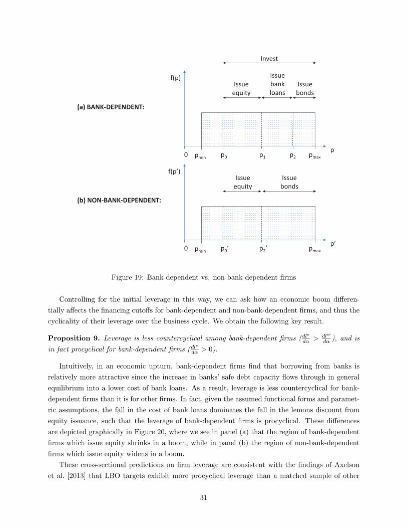
sections, depicted in panel (a) of Figure 19. In particular, now the worst quality entrepreneurs

issue equity, moderate quality entrepreneurs issue bank loans, and high quality entrepreneurs issue

bonds. We obtain the following statement of equilibrium.

Proposition 8. Under Assumptions 4 and 5, there exists an equilibrium in which:

• entrepreneurs sort as follows:

– p ∈ [p2, pmax] invest, fully commit their own capital ce, and issue zD = 1− ce in bonds;

– p ∈ [p1, p2) invest, fully commit their own capital ce, and issue zB = 1−ce in bank loans;

– p ∈ [p0, p1) invest, fully commit their own capital ce, and issue zE = 1− ce in equity;

– p ∈ [pmin, p1] do not invest;

• bankers act as follows:

29

(a)

BROKER/DEALER

(b)

COMMERCIAL BANK

0 lb

1+rb

(1+r)(1+ms)

b(mu) = 0

b(ms) = 0

1 0

lb 1

b(mu) = 0 b(ms) = 0

1+rb

(1+r)(1+ms)

Figure 18: Impact of an economic downturn

– skilled bankers intermediate, financing every dollar of assets with zS = z̄S(rb;ms), zD =

lb − z̄S(rb;ms), and zE = 1− lb;

– unskilled bankers do not intermediate;

and {p0, p1, p2, 1 + rb, lb} are characterized by the system:

12(1− p2)d = rb − r(1 + r)

(v(p1)v(p0)

)= 1 + rb(

1− (1+r)(1−ce)v(pE)

)v(p0) = (1 + r)ce

lb = z̄S(rb;ms) + (1− zS) 1

1+12 d

1+r

1+rb

1+ms = 1 + r + 12d(lb − z̄S(rb;ms))

,

where pE ≡ E[p|p ∈ [p0, p1]], z̄S(rb;ms) = 1

1+rγsd

(1+rb

1+ms

), and γsd = E

[p

12+ 1

2p|p ∈ [p1, p2]

].

We can now compare these firms’ behavior to those of firms with the same level of leverage,

but which do not rely on any bank financing. That is, consider the entrepreneurs in panel (b) of

Figure 19. For the cutoff between equity and bank loans for bank-dependent firms to be the same

as the cutoff between equity and bonds for non-bank-dependent firms, the latter must have a lower

cost of financial distress but prohibitively high monitoring costs. This is formalized below.

Corollary 2. Consider two groups of firms across which banks cannot diversify. Bank-dependent

firms are defined as in the previous proposition, while non-bank-dependent firms face a cost of

financial distress d′ but prohibitively expensive monitoring costs ms′,mu′ → ∞, such that these

firms are only equity and bond-financed. Then there exists a unique d′ < d such that p0 = p′0,

p1 = p′2, and thus le = le′.

30

p 0 p2

Invest

Issue

bank

loans

Issue

bonds

f(p)

pmax pmin p1 p0

Issue

equity

p’ 0

Issue

bonds

f(p’)

pmax pmin p2’ p0’

Issue

equity

(a) BANK-DEPENDENT:

(b) NON-BANK-DEPENDENT:

Figure 19: Bank-dependent vs. non-bank-dependent firms

Controlling for the initial leverage in this way, we can ask how an economic boom differen-

tially affects the financing cutoffs for bank-dependent and non-bank-dependent firms, and thus the

cyclicality of their leverage over the business cycle. We obtain the following key result.

Proposition 9. Leverage is less countercyclical among bank-dependent firms (dle

dα > dle′

dα ), and is

in fact procyclical for bank-dependent firms (dle

dα > 0).

Intuitively, in an economic upturn, bank-dependent firms find that borrowing from banks is

relatively more attractive since the increase in banks’ safe debt capacity flows through in general

equilibrium into a lower cost of bank loans. As a result, leverage is less countercyclical for bank-

dependent firms than it is for other firms. In fact, given the assumed functional forms and paramet-

ric assumptions, the fall in the cost of bank loans dominates the fall in the lemons discount from

equity issuance, such that the leverage of bank-dependent firms is procyclical. These differences

are depicted graphically in Figure 20, where we see in panel (a) that the region of bank-dependent

firms which issue equity shrinks in a boom, while in panel (b) the region of non-bank-dependent

firms which issue equity widens in a boom.

These cross-sectional predictions on firm leverage are consistent with the findings of Axelson

et al. [2013] that LBO targets exhibit more procyclical leverage than a matched sample of other

31

p1

p0 0

p0(p2)

p1(p0)

(a)

BANK-DEPENDENT

p2’

p0’ 0

p0’(p2’)

p2’(p0’)

(b)

NON-BANK-DEPENDENT


non-financial firms, as LBO financing is heavily dependent on the syndicated loan market. They

are also consistent with the findings in Leary [2009] that smaller, bank-dependent firms exhibit

more procyclical leverage than larger, less bank-dependent firms.

Proposition 9 also makes an interesting and testable cross-country prediction. In particular, it

would predict that holding the initial level of leverage the same, firms in bank-dependent economies

(e.g., Europe) should exhibit more procyclical leverage than those in non-bank-dependent economies

(e.g., the U.S.). I leave an empirical test of this prediction to future work.

6 Welfare and policy

Having demonstrated the positive explanatory power of the framework developed in this paper, I

now study its normative implications. I first characterize the constrained efficient allocation chosen

by a planner constrained by the same technological and informational frictions as agents in the

economy. I then show that there is a role for macroprudential policy in limiting the level, but not

cyclicality, of bank leverage to implement the constrained efficient allocation.

6.1 Constrained efficiency

Consider a planner focused on the intermediation chain involving bankers studied in section 4, and

who is restricted to selecting one among the feasible allocations supported as competitive equilibria

following Definition 3. This planner then is constrained by the same technological and informational

frictions as agents in the economy, but has the power to choose any one of the multiple equilibria.

I define a constrained efficient allocation to be one chosen by this planner to maximize ex-ante

utilitarian social welfare.10 Given linear and identical preferences across agents, this welfare metric

10It is well known that in signaling models in the tradition of Spence [1973], the set of multiple equilibria often can

32

0 lb

1+rb

(1+r)(1+ms)

1

Constrained efficient equilibria,

implemented by leverage cap

b(mu) = 0 b(ms) = 0

Equilibrium

under study

C

E D

A B

Figure 21: Constrained efficiency and implementation in banking

is simply given by the NPV of investment, less monitoring costs and expected costs of financial

distress, plus initial wealth in the economy. The following result characterizes the equilibria which

achieve the constrained efficient allocation according to this definition.

Proposition 10. In the constrained efficient equilibria, entrepreneurs sort as in Proposition 5,

bankers act as follows:

• skilled bankers intermediate, financing every dollar of assets with zS,ce ≤ z̄S(rb,ce;ms) ≡1

1+rγsd

(1+rb,ce

1+ms

), zD,ce = 0, and zE,ce = 1− zS,ce;

• unskilled bankers may or may not intermediate;

and {pce1 , pce2 , 1 + rb,ce} are characterized as follows:12(1− pce2 )d = rb,ce − rv(pce1 ) = 1 + r + (rb,ce − r)(1− ce)1 + rb,ce = (1 + r)(1 +ms)

.

These equilibria are depicted in Figure 21, and are compared with the benchmark equilibrium

under study in section 4 (at point C).

In the constrained efficient equilibria, the equilibrium interest rate on bank loans simply com-

pensates bankers for the cost of monitoring. The ROA of skilled bankers is thus 1 + r, and their

equilibrium financing is simply composed of safe debt (deposits) and equity. Because skilled bankers’

ROA is identical to that of unskilled bankers, there is no incentive for the latter to imitate the for-

mer, and the equity of skilled bankers will be fairly priced. Hence, bankers’ weighted average cost

of capital is 1 + r, ensuring that the zero profit condition is satisfied. Indeed, within the class of

be Pareto ranked. My definition of the constrained efficient allocation in this setting identifies a particular equilibriumor set of equilibria on the Pareto frontier — namely, that/those which maximize ex-ante utilitarian social welfare.

33

financing structures using only safe debt and equity, bank financing is indeterminate following the

Modigliani and Miller [1958] Theorem.

Relative to the constrained efficient allocation, the equilibrium studied in section 4 features fewer

positive-NPV entrepreneurs receiving financing and greater deadweight costs of bond financing. As

such, not only does the constrained efficient allocation yield higher ex-ante utilitarian social welfare

— it Pareto dominates the equilibrium of section 4. Moving from the latter to the former, previously

bank-financed and newly bank-financed entrepreneurs see their expected profit strictly increase,

while all other entrepreneurs find that their profit has not changed. Bankers and households

continue to earn zero profits and (1 + r)ch, respectively.

Coordination at the inefficient equilibrium of section 4 is sustained by asymmetric information.

In particular, at a high interest rate on bank loans, skilled bankers attempt to signal their quality

to the market by issuing costly, risky debt which unskilled bankers cannot profitably replicate. The

act of issuing costly, risky debt raises skilled bankers’ weighted average cost of capital, supporting

the high interest rate on bank loans in an equilibrium with free entry into banking. No skilled

banker seeks to issue less risky debt, and thus charge a lower interest rate on bank loans and

capture the market, for fear that doing so would signal he is unskilled.

6.2 Implementation through macroprudential regulation

In practice, the observation that banks issue massive quantities of short-term financing suggests

that we may indeed live in a world that has coordinated on the inefficient equilibrium discussed

above. While the distinction between safe and risky short-term debt is admittedly imprecise, if we

interpret at least some of these short-term debt securities as costly attempts to signal quality to

the market, this model suggests that there can exist a socially excessive incentive to do so.

Starting from the inefficient equilibrium, Figure 21 suggests that a simple macroprudential tool

can implement the constrained efficient allocation: a cap on bank leverage. Similar to results in

other signaling models where banning signaling can generate a Pareto improvement, a leverage cap

can break coordination at a ‘high interest rate - high leverage’ equilibrium. Formally, we have:

Proposition 11. A banking leverage cap of l̄b = z̄S(rb,ce;ms) can eliminate all equilibria in the

banking sector except those leading to the constrained efficient allocation.

At the same time, because banks’ safe debt capacity remains procyclical in the constrained effi-

cient allocation, the model does not justify the use of macroprudential tools to limit this cyclicality.

The intuition is unchanged from the equilibrium of section 4: banks are diversified intermediaries

whose worst-case payoff rises when idiosyncratic project quality in the economy improves.

Indeed, within the set of constrained efficient equilibria, there are reasons outside the model to

think that letting banks issue as much safe debt as possible may be uniquely constrained efficient.

In particular, there appears to exist a special demand for banks’ safe liabilities — whether because

they provide the transaction services of money (a la Stein [2012]), or because they cater to a specific

investor clientele (pension funds, etc.) in a world of segmented markets.

34

To that end, the following result is notable.

Proposition 12. The safe debt capacity of banks in the constrained efficient equilibria z̄S(rb,ce;ms)

is procyclical: ddα z̄

S(rb,ce;ms) > 0. Thus, implementing the constrained efficient equilibrium with

maximal safe debt issuance requires a time-varying, procyclical leverage cap.

Other authors have also advocated for time-variation in bank regulation; what is notable about

this result is that bank leverage regulation should be looser in good times, to accommodate time

variation in the safe debt capacity in the banking sector. To be sure, proponents of countercyclical

leverage requirements (e.g., Hanson et al. [2011]) have in mind dynamic trade-offs and pecuniary

externalities which the present model does not capture. Nonetheless, the analysis here demonstrates

that time variation in banks’ capacity to issue safe debt is an important force which should also be

taken into account in the analysis of macroprudential regulation.

7 Conclusion

This paper jointly characterizes the investment and financing of non-financial firms and banks in

general equilibrium. It is designed to explain the differential cyclicality of firm and bank leverage

over the business cycle. The core idea is that while firm leverage falls in an economic boom because

of a lower lemons discount in equity issuance relative to the costs of financial distress, bank leverage

rises because banks, as diversified intermediaries, see their capacity to issue safe debt expand.

I use this framework to then illuminate several other stylized facts in the data and questions

of welfare and policy. First, the model rationalizes the weaker procyclicality of commercial bank

leverage as arising from deposit insurance: such insurance reduces the volatility in safe debt capacity

for commercial banks relative to that for uninsured intermediaries such as broker/dealers. Second,

the model rationalizes evidence on the procyclicality of leverage for LBO targets and small firms:

such bank-dependent firms inherit the improved funding conditions of banks in a boom due to

a general equilibrium effect on the cost of bank loans. Finally, the model motivates a role for

macroprudential regulation of the level of bank leverage, but not its cyclicality. The latter follows

from the fact that bank issuance of safe debt is a constrained efficient response to informational

and technological frictions in the economy, and their capacity to issue safe debt is procyclical.

A fruitful direction for future work is to enrich the present framework with durable goods,

permitting the modeling of pecuniary externalities. This might introduce a rich trade-off in the

determination of time-varying capital requirements for banks: on the one hand, preventing banks

from shedding assets and delevering in a downturn might avoid socially costly pecuniary externali-

ties, but on the other, forcing banks to maintain higher capital ratios in a boom might complicate

their issuance of socially beneficial safe debt. Analyzing this trade-off through an enriched version

of the present framework may shed light on comparative statics and empirical moments which can

guide policymakers in balancing these objectives to optimally regulate bank capital over the cycle.

35

References

Tobias Adrian and Hyun Song Shin. Liquidity and leverage. Journal of Financial Intermediation,

19(2010):418–437, 2010a.

Tobias Adrian and Hyun Song Shin. The changing nature of financial intermediation. Federal

Reserve Bank of New York Staff Reports, 439:1–34, 2010b.

Tobias Adrian and Hyun Song Shin. Financial intermediary balance sheet management. Federal

Reserve Bank of New York Staff Reports, 532:1–28, 2011.

Tobias Adrian and Hyun Song Shin. Procyclical leverage and value-at-risk. Review of Financial

Studies, 27(2):373–403, 2014.

Ulf Axelson, Tim Jenkinson, Per Stromberg, and Michael S. Weisbach. Borrow cheap, buy high?

The determinants of leverage and pricing in buyouts. Journal of Finance, 68(6):2223–2267, 2013.

Patrick Bolton and David S. Scharfstein. Optimal debt structure and the number of creditors.

Journal of Political Economy, 104(1):1–25, 1996.

Markus K. Brunnermeier and Martin Oehmke. The maturity rat race. Journal of Finance, 68(2):

483–521, 2013.

Charles W. Calomiris and Charles M. Kahn. The role of demandable debt in structuring optimal

banking arrangements. American Economic Review, 81(3):497–513, 1991.

In-Koo Cho and David M. Kreps. Signaling games and stable equilibria. Quarterly Journal of

Economics, 102(2):179–221, 1987.

Hyuk Choe, Ronald W. Masulis, and Vikram Nanda. Common stock offerings across the business

cycle: Theory and evidence. Journal of Empirical Finance, 1(1993):3–31, 1993.

Douglas W. Diamond. Financial intermediation and delegated monitoring. Review of Economic

Studies, 51(3):393–414, 1984.

Douglas W. Diamond and Philip H. Dybvig. Bank runs, deposit insurance, and liquidity. Journal

of Political Economy, 91(3):401–419, 1983.

Douglas W. Diamond and Raghuram G. Rajan. A theory of bank capital. Journal of Finance, 55

(6):2431–2465, 2000.

Mark J. Flannery. Debt maturity and the deadweight costs of leverage: Optimally financing banking

firms. American Economic Review, 84(1):320–331, 1994.

Evan Gatev and Philip E. Strahan. Banks’ advantage in hedging liquidity risk: Theory and evidence

from the commercial paper market. Journal of Finance, 61(2):861–892, 2006.

36

John Geanakoplos. The leverage cycle. NBER Macroeconomic Annual 2009. University of Chicago

Press, 2010.

Nicola Gennaioli, Andrei Shleifer, and Robert W. Vishny. A model of shadow banking. Journal of

Finance, 68(4):1331–1363, 2013.

Gary Gorton and George Pennacchi. Financial intermediaries and liquidity creation. Journal of

Finance, 45(1):49–71, 1990.

Samuel G. Hanson, Anil K. Kashyap, and Jeremy C. Stein. A macroprudential approach to financial

regulation. Journal of Economic Perspectives, 25(1):3–28, 2011.

Zhiguo He and Arvind Krishnamurthy. Intermediary asset pricing. American Economic Review,

20(20):1–42, 2012.

Zhiguo He, In Gu Khang, and Arvind Krishnamurthy. Balance sheet adjustments in the 2008 crisis.

IMF Economic Review, 58:118–156, 2010.

Victoria Ivashina and David S. Scharfstein. Bank lending during the financial crisis of 2008. Journal

of Financial Economics, 97(3):319–338, 2010.

Mark T. Leary. Bank loan supply, lender choice, and corporate capital structure. Journal of

Finance, 64(3):1143–1185, 2009.

Franco Modigliani and Merton H. Miller. The cost of capital, corporation finance and the theory

of investment. American Economic Review, 48(3):261–297, 1958.

Stewart C. Myers. The capital structure puzzle. Journal of Finance, 39(3):575–592, 1984.

Stewart C. Myers and Nicholas S. Majluf. Corporate financing and investment decisions when firms

have information that investors do not have. Journal of Financial Economics, 13(2):187–221,

1984.

Andrei Shleifer and Robert W. Vishny. The limits of arbitrage. Journal of Finance, 52(1):35–55,

1997.

Alp Simsek. Belief disagreements and collateral constraints. Econometrica, 81(1):1–53, 2013.

Clifford W Smith, Jr. and Jerold B. Warner. On financial contracting: An analysis of bond

covenants. Journal of Financial Economics, 7(1979):117–161, 1979.

Michael Spence. Job market signaling. Quarterly Journal of Economics, 87(3):355–374, 1973.

Jeremy Stein. Monetary policy as financial stability regulation. Quarterly Journal of Economics,

127(1):57–95, 2012.

Robert M. Townsend. Optimal contracts and competitive markets with costly state verification.

Journal of Economic Theory, 21:265–293, 1979.

37

Proofs†

Proposition 3: equilibrium in non-financial corporate sector

Proof. Demonstrating that the conjectured equilibrium is in fact an equilibrium requires showing

that (i) the parametric conditions in Assumption 4 ensure that {p2, p0} solving (1) and (2) exist,

and (ii) there exist off-path beliefs under which all entrepreneurs are indeed acting optimally.

I start with (i). By the implicit function theorem, let p(1)2 (p0) be the upward-sloping schedule

defined by (1) and let p(2)2 (p0) be the downward-sloping schedule defined by (2). Then we have

pnpv = p(2)2 (pnpv) < p

(1)2 (pnpv) ∈ (pnpv, pmax),

where the last relation follows from

0 < d

by Assumption 4. And we have

∞ = p(2)2 (p) > pmax > p

(1)2 (p)

for p := v(p) = (1 + r)ce, where the last relation follows from the fact that

d <(1 + r)

(v(pmax)

v(E[p|p∈[pnpv ,pmax]]) − 1)

12(1− pmax)

<

(1 + r)

(v(pmax)

v(E[p|p∈[p,pmax]])− 1

)12(1− pmax)

by Assumption 4. Since we know pnpv ∈ (pmin, pmax) and p ∈ (pmin, pnpv) following

v(pmin)

1 + r< ce < 1 <

v(pmax)

1 + r

the Intermediate Value Theorem guarantees that there exists a (unique) {p0 ∈ (p, pnpv), p2 ∈(p0, pmax)} solving

p(2)2 (p0) = p

(1)2 (p0).

Now I turn to (ii). Consider the following off-path beliefs:

• If zE + zD = 1− ce,µ(p|zE , zD) = f(p|p ∈ [p0, p2]).

• If zE + zD > 1− ce,

µ(p|zE , zD) = δ{p = max{pmin, p∗(zD)}}, where p∗(zD) := v(p∗) = (1 + r +1

2(1− p∗)d)zD.

†I provide proofs of results for which the intuition is not fully laid out in the main text. Formal proofs of resultsnot provided here are available on request.

38

Note that here δ is the Dirac delta function. Under these beliefs, for entrepreneurs who seek

1 − ce in external financing, households’ posterior is that they are just like equity issuers in the

conjectured equilibrium. But for entrepreneurs who seek more than 1 − ce in external financing,

households’ posterior is quite pessimistic, consistent with the intuition that “high” types would

seek to minimize external finance since frictions render it costly. In particular, their posterior in

this case assigns entrepreneurs to be the lowest type who could in fact raise zD in debt. This latter

condition ensures that beliefs are “reasonable” in the present setting where households should be

able to backward induce from entrepreneurs’ ability to raise informed capital (debt) their minimum

type. Assumption 4 implies that

1 + r + 12(1− pmin)d

2(1 + r) + 12(1− pmin)d

< ce ⇒1 + r + 1

2(1− p)d2(1 + r) + 1

2(1− p)d< ce ⇒ v(p0) > (1 + r +

1

2(1− p)d)(1− ce),

ensuring that even entrepreneur p0 could raise up to zD = 1− ce in informed capital.

It is straightforward to verify that under these beliefs, all entrepreneurs are acting optimally.

Proposition 4: countercyclical leverage in non-financial corporate sector

Proof. Let F̃ be the CDF of the transformation p̃ ≡ p−pmin

pmax−pmin. Then following Definition 1,

F̃ (p̃) = p̃α (the CDF of a Beta(α, 1) random variable), and we are interested in the effect of local

changes in α around α = 1 (the U [0, 1] case).

Since assets and leverage are

ae = 1− F (p0) = 1− p̃α0 ,

le =1− F (p2)

1− F (p0)(1− ce) =

1− p̃α21− p̃α0

(1− ce),

for p̃0 ≡ p0−pmin

pmax−pminand p̃2 ≡ p2−pmin

pmax−pmin, it is straightforward to show

dae

dα∝ −dp̃0

dα

α

p̃0− ln p̃0,

dle

dα∝ (1− p̃α2 )p̃α0

(dp̃0dα

α

p̃0+ ln p̃0

)− (1− p̃α0 )p̃α2

(dp̃2dα

α

p̃2+ ln p̃2

).

Differentiating the system (1) and (2), we can show:

• dp2dα

αp2> 0, which remains bounded above zero even for d (and ce) on the high end of their

respective ranges in Assumption 4,

• dp0dα

αp0< 0.

The second point immediately implies that dae

dα > 0. And when d is on the high end of its range in

Assumption 4, so p̃2 is close to its upper bound 1 and thus initial leverage is low, we have that dle

dα

takes the sign of −dp̃2dα ∝ −

dp2dα < 0.

39

Proposition 5: equilibrium in banking

Proof. Demonstrating that the conjectured equilibrium is in fact an equilibrium requires showing

that (i) the parametric conditions in Assumption 5 ensure that {p1, p2, 1 + rb, lb} solving (3), (4),

(5), and (6) exist, and (ii) there exist off-path beliefs under which all bankers are indeed acting

optimally.

I start with (i). First note that we can combine (5) and (6) to obtain (7), and then can plug

the latter into (3) and (4), to obtain the system

1

2(1− p2)d = (1 + r)

(1 +ms)

1 +12d

1+r+ 12d

1 +12d

1+r+ 12dγsd

− 1

, (8)

v(p1) = (1 + r)

1 + (1− ce)

(1 +ms)

1 +12d

1+r+ 12d

1 +12d

1+r+ 12dγsd

− 1

, (9)

γsd = E

[p

12 + 1

2p|p ∈ [p1, p2]

]. (10)

Hence, if we can prove that {p1, p2, γsd} solving this smaller system exist, we are done.

I will focus on the parametric case of small ms and d, following Assumption 5. First note that

given ∂∂p2

γsd < 1 by Assumption 5, we can use the Implicit Function Theorem to argue that (8)

implies the well-defined function p2(p1) over p1 ∈ [pnpv, pmax) which is upward-sloping for ms and

d small. In fact, as ms, d→ 0, the fact that χ ≡ ms

d satisfies

1

2

1

1 + r

(E

[p

12 + 1

2p|p ∈ [pnpv, pmax]

]− pmax

)< χ <

1

2

1

1 + r

((pnpv

12 + 1

2pnpv

)− pnpv

)

(by Assumption 5) implies that p2(p1) converges to an upward-sloping function p2(p1) where

p2(pnpv) ∈ (pnpv, pmax).

We can then use the Implicit Function Theorem to argue that (9) implies the well-defined function

p1(p2) over p2 ∈ (pnpv, pmax] which is downward-sloping. And as ms, d → 0, p1(p2) converges to

the constant

p1 = pnpv.

It follows that {p1 = pnpv, p2 = p2(pnpv)} solve the system of limiting equations asms and d converge

to zero and χ remains in the range above. Since the conditions (8)-(10) are all well-behaved, it

follows that for small but positive ms and d, the upward-sloping p2(p1) and downward-sloping

p1(p2) intersect near the point {p1 = pnpv, p2 = p2}, and an equilibrium exists.

40

Now I turn to (ii). Consider household beliefs

µ

ms|lb < z̄S(rb;ms) + (1− z̄S(rb;ms))1

1 +12d

1+r

= 0,

µ

ms|lb ≥ z̄S(rb;ms) + (1− z̄S(rb;ms))1

1 +12d

1+r

= 1,

where µ satisfies as well the conditions of Lemma 3. Under these beliefs, a household perceives a

low-leverage issuer to be unskilled with probability one, and a sufficiently high-leverage issuer to

be skilled with probability one. These beliefs reflect the intuition that only the (more profitable)

skilled bankers can afford to undertake the costly signal of issuing risky debt.

It is straightforward to verify that under these beliefs, all bankers are acting optimally.

Proposition 6: procyclical leverage in banking

Proof. First differentiate the system (8)-(10), which given the conditions of Assumption 5 can be

used to show that for ms, d small:

• dγsddα > 0,

• dp2dα > 0, is bounded above zero even as ms, d → 0, and remains bounded above zero even if

χ ≡ ms

d is arbitrarily close to the bottom of the range in Assumption 5,

• dp1dα < 0 but converges to zero as ms, d→ 0.

Then with respect to bank leverage,

dlb

dα∝ d

dαz̄S(rb;ms),

∝ d

dαγsd,

> 0,

where the first line uses (5) and the second line uses (7) (which simply combines (5) and (6)).

And with respect to bank assets

ab = (F (p2)− F (p1))(1− ce)(1 +ms),

= (p̃α2 − p̃α0 )(1− ce)(1 +ms),

where the second line uses the definition of the transformations used extensively in the proof of

Proposition 4, we have that

dab

dα∝ p̃α2

(dp̃2dα

α

p̃2+ ln p̃2

)− p̃α1

(dp̃1dα

α

p̃1+ ln p̃1

).

41

Hence, dab

dα > 0 when χ is near the bottom of the range in Assumption 5, and thus p̃2 is near the

upper bound 1, and thus the initial share of bank loans in credit provision is sufficiently high.

Proposition 10: constrained efficient equilibria

Proof. Relative to the problem facing the constrained planner described in the text, consider a

relaxed problem in which the planner can directly choose the consumption, investment, and fi-

nancing decisions of entrepreneurs, banks, and households subject only to the economy’s aggregate

resource constraints and the technological constraints posed by the investment technology of each

entrepreneur and the deadweight costs involved in bank loan and bond financing.

It is first straightforward to see that this planner will not have banks issue any risky debt, as

this would increase the social costs of financing with no social benefit. With this in mind, and

given the linear preferences of each agent, the aggregate resource constraints for the economy at

each date mean that the planner with ex-ante utilitarian objective faces

max1{invest}(p),zB(p),zD(p)

[ce +Hch −

∫ pmax

pmin

1{invest}(p)[1 +mszB(p)]dp

]+

β

[∫ pmax

pmin

1{invest}(p)[v(p)− 1

2(1− p)dzD(p)]dp

]s.t.

zB(p) + zD(p) ≥ 1− ce, ∀p.

It is straightforward to see that the solution to this program has the bang-bang nature

1{invest}(p) = 1 iff v(p) ≥ 1

β+ min{m

s

β,1

2(1− p)d}(1− ce),

zB(p) = 1− ce iff 1{invest}(p) = 1 andms

β<

1

2(1− p)d,

zD(p) = 1− ce iff 1{invest}(p) = 1 andms

β>

1

2(1− p)d.

Then note that in the competitive equilibria under study, 1 + r = 1β . It follows that the

above allocation can be achieved in the feasible set (the set of allocations supported as competitive

equilibria following Definition 3), as outlined in the claim and depicted in Figure 21. Hence, this

allocation is in fact constrained efficient as well.

Proposition 11: implementation of constrained efficiency through leverage cap

Proof. Recall that by Lemma 2 we have 1 + rb ≥ (1 + r)(1 +ms) in any equilibrium, and following

Lemma 3 I will restrict the analysis only to equilibria with bank diversification.

First suppose there exists an equilibrium with 1+rb > (1+r)(1+ms) and lb ≤ lb ≡ z̄S(rb,ce;ms).

If such an equilibrium is a separating one, skilled banks earn positive profit which is inconsistent

with free entry. If such an equilibrium is a pooling one, unskilled banks earn positive profit (from

a subsidy from equity issuance) which is inconsistent with free entry. Hence, by contradiction no

42

such equilibrium exists.

Next suppose that there exists an equilibrium with 1 + rb = (1 + r)(1 + ms) and lb ≤ lb ≡

z̄S(rb,ce;ms). Given this value of 1 + rb, {p1, p2} are determined by (3) and (4), and in particular

we have p1 = pce1 and p2 = pce2 . Since lb ≤ lb ≡ z̄S(rb,ce;ms), it is clear this equilibrium achieves

the constrained efficient allocation as described in Proposition 10.

43

Firm vs. Bank Leverage over the Business...

Documents

Transcript of Firm vs. Bank Leverage over the Business...