Firm Value and Corporate Governance -...

Firm Value and Corporate Governance:

How the Former Determines the Latter∗

Benjamin E. Hermalin†

Abstract

A model of corporate governance must explain (i) why governancematters; (ii) variation in governance across firms (i.e., be responsiveto the Demsetz and Lehn, 1985, critique); and (iii) the positive cor-relations found empirically between quality of corporate governanceand corporate performance. The model presented here satisfies thesethree criteria. Moreover, the model explains the correlation betweenfirm size and executive compensation and why empirical estimatesof managerial incentives seem too low, among other phenomena.

Keywords: corporate governance, executive compensation, firm het-erogeneity, trends in governance.

∗The author thanks seminar participants at the Universities of Arizona, California (Berke-ley), Chicago, and Missouri, Ohio State University, and the 13th Finsia Conference, Mel-bourne, for valuable feedback on earlier versions. As usual, they are exonerated with respectto the paper’s residual shortcomings. The financial support of the Thomas and Alison Schnei-der Distinguished Professorship in Finance is gratefully acknowledged.

†University of California • Walter A. Haas School of Business • S545 Student ServicesBuilding #1900 • Berkeley, CA 94720–1900. email: [email protected].

Draft 11/11/2008—Version 11

Contents

Contents

1 Introduction 1

2 The Basic Model 4

3 Endogenous Investment 9

4 Managerial Compensation 12

5 Alternative Formulations 17

6 Trends in Governance 21

7 Conclusions 23

Appendix A: Proofs 25

Appendix B: Issues in Estimating Pay for Performance 28

References 31

i

Introduction 1

1 Introduction

As a rule, people choose more security or protection the more they have at stake.Observations of homeowners, merchants, and institutions support this view:those with more at stake typically have greater security. The same rule shouldapply to firm owners when they must rely on others to manage their firms. Aconcern, dating at least as far back as Adam Smith, is that managers will abuse,misuse, or even misappropriate the resources of the firm.1 Corporate governanceis the security that owners put in place to protect their interests against suchagency problems. It is well-documented that the strength of governance variesacross firms; and one might ask which firms will have stronger governance thanothers? The answer, I will argue, are those in which more is at stake.

Which firms have more at stake? To an extent, those with the most resources(e.g., capital, assets, etc.). But also those that possess the greatest potentialreturn to those resources. Specifically, consider two firms, A and B, with Bhaving the greater marginal return to resources. The marginal cost to B’sowners of an abused, misused, or misappropriated dollar of resources is, thus,greater than it is for A’s. Consequently, the marginal return to B’s owners ofinvesting in greater security—that is, stronger corporate governance—is greaterthan it is for A’s. In equilibrium, firm B will have stronger governance thanfirm A. Furthermore, if the factors that give firm B greater marginal returnsalso directly increase its returns, then firm B will be more profitable than firm Ain equilibrium. Profits and strength of governance will, therefore, be positivelycorrelated. Observe that this correlation follows not because better governanceleads to greater profitability. Rather it follows because potential profitabilityleads to better governance.2

This view satisfies the three requirements necessary of theory in this area:(i) it must allow governance to matter; (ii) it must explain why there is varia-tion in governance across firms; and (iii) it must also explain why we observethe empirical results we do; in particular, that in many studies—but not all—there is a positive correlation between stronger governance and firm performance(profitability or value).3 The idea that A’s profit potential is worse than B’s isparticularly attractive with respect to these last two criteria because it readilyexplains both why A’s owners choose weaker governance than B’s and why thelevel of governance and firm performance are positively correlated.

1“The directors of companies, however, being the managers rather of other people’s moneythan of their own, it cannot well be expected, that they should watch over it with the sameanxious vigilance . . . negligence and profusion, therefore, must always prevail, more or less, inthe management of the affairs of such a company.” — Smith (1776).

2Causality is an important, but vexing, issue in the study of corporate governance. Demsetzand Lehn (1985) were among the first to make this point. Others who have raised it includeHimmelberg et al. (1999), Palia (2001), Hermalin and Wallace (2001), and Coles et al. (2007).The point has also been discussed in various surveys of the literature; consider, e.g., Bhagatand Jefferis (2002), Becht et al. (2003), and Hermalin and Weisbach (2003) among others.

3See the literature surveys by Becht et al. and Hermalin and Weisbach for examples anddiscussion.

Introduction 2

The more-to-protect view developed here is an alternative to the more preva-lent views in the literature, which tend to be cost-based. For instance, variationin the noisiness of a firm’s environment affects contracting costs, which in turndetermine the degree to which agency problems are ameliorated, thus finally de-termining performance (Demsetz and Lehn; Himmelberg et al.; Palia; and Her-malin and Wallace); or variation in the complexity and size of a firm’s operationsaffect contracting costs and, hence, agency amelioration and firm performance(Demsetz and Lehn; Himmelberg et al.; and Hermalin and Wallace).

The two views can be summarized as (i) firms vary in their profit potential sothat firms with greater potential ceteris paribus have a higher marginal return togovernance; or (ii) firms vary on the cost side so that firms with lower marginalcosts of governance have more of it and, therefore, higher profits.4 At onelevel, as discussed in Section 5.2 below, a similar logic is behind both stories.Ultimately, whether it is heterogeneity on the profit-side or the cost-side thatis more important is an empirical question. As discussed in Sections 5.2 and 6,the trend toward stronger governance over the past quarter century or so wouldsuggest it is primarily the profit-side that is critical given that the empiricalevidence suggests that the marginal cost of governance has, if anything, risenover this period.

Another reason to consider the profit-potential side is that one might expectfirms in the same industry to face similar agency costs. Yet, intra-industry het-erogeneity in governance is large (see, e.g., Hermalin, 1994, and Hermalin andWallace, 2001, for discussion and evidence). Although within-industry compe-tition itself can account for some of this heterogeneity (Hermalin, 1994), thefact that different firms have different profit potentials (e.g., as a consequenceof valuable intellectual property, superior location, advantageous supplier rela-tions, etc.) offers another explanation.

Yet another reason to consider the profit-side perspective is that firm size,which is often taken to be a cost determinant, is itself endogenous. As discussedbelow, heterogeneity on the profit-side can explain both firm size and the levelof governance.

One paper that can be seen as also considering the profit-side is the con-temporaneous work of Coles et al. Although their paper is primarily empirical,it does contain a brief model of optimal managerial ownership in which thefirm’s productivity, among other factors, influences the amount of managerialownership. They do not, however, analyze the general relation between profitpotential and governance; nor do they distinguish between marginal and leveleffects.

In what follows, Section 2 presents the model. The key assumption is thatfirms vary in their marginal returns from resources utilized for the owners’ ben-efit (i.e., total resources less those diverted by the manager). It is shown that

4It is worth noting that the cited articles, which provide primarily verbal models, do notdistinguish between total and marginal costs of governance. For a variety of reasons (see, e.g.,

Grossman and Hart, 1983 or Hermalin, 1994), comparative statics on the cost side can oftenbe quite subtle or counter-intuitive; in particular, a factor that raises total cost might noteverywhere shift the marginal-cost schedule in the same direction.

Introduction 3

firms with higher marginal returns—higher-type firms—will have stronger gov-ernance than those with lower marginal returns—lower-type firms. If type alsodirectly and positively affects profits, then there will be a positive correlationbetween profits and the level of governance; however, the correlation is essen-tially spurious in that both variables are positively correlated with firm type(profit potential).

Section 2 also considers the situation in which firms are homogeneous in type,but vary with respect to total resources. The more-to-protect rule is shown toapply here too: firms with more resources will tend to have stronger governanceand greater profits. Again, governance and profits are positively correlated, butalso again the correlation is spurious—both variables are a function of totalresources.

In Section 2, a firm’s total resources are fixed exogenously. In many contexts,it is better to think of them as endogenously determined, with the necessaryfunds coming from the capital markets. Section 3 extends the basic modelto allow the firm’s owners to also determine how much capital is to be raised.Higher-type firms will raise more capital, have stronger governance, and generategreater profits than will lower-type firms. To the extent the amount of capitalraised or profits are indicators of firm size or correlated with other measures ofsize, the results from this section predict a positive correlation between firm sizeand the strength of governance. It is also shown that the level of governancecould well be independent of a firm’s capital structure.

A particularly important form of governance is incentive compensation. Sec-tion 4 explores the implications of the model for compensation. It is shown therethat higher-type firms pay more in expectation than lower-type firms; that is,executives are paid more not only as a function of how their firms actually do,but also as a function of how they are expected to do. Given that profits arecorrelated with standard measures of firm size, this insight offers a novel expla-nation for the positive correlation between firm size and executive pay commonlyfound in the data.

Much of Section 4 concerns the standard cross-sectional regression of payon performance. It is shown that equation is almost always misspecified. Im-portantly, this misspecification leads to the coefficient on performance (profit)being biased downward so that it understates the true strength of the incentivesexecutives have. This finding sheds light on the debate over whether real-lifeexecutives are given sufficiently strong incentives.

Section 5 considers two alternative formulations of the model. One, as dis-cussed above, considers heterogeneity on the cost side of governance. The other,considered in Section 5.1, addresses the degree to which the analysis of the earliersections continues to hold if governance is a multi-dimensional variable. That is,in that section, the fact the governance can vary simultaneously across firms onmany dimensions, such as board structure, incentive compensation, shareholderactivism, and so forth, is explicitly considered. It is readily shown that firmswith better profit potentials will spend more on governance than firms withweaker profit potentials. This does not, however, mean that higher-type firmshave stronger governance on all dimensions. Such a result follows, however, if

The Basic Model 4

it is assumed that there is complementarity in governance.Section 6 contains a brief discussion of how the analysis in this paper sheds

light on trends in corporate governance over the past twenty to thirty years.Section 7 is a brief conclusion, which focuses on the implications of the analysisfor future empirical work in the area.

Because much of the analysis involves a reduced-form model, it is importantto note that the model in question can be derived from first principles. Anearlier version of this paper developed two models from first principles thatcorrespond to the reduced-form model used in the main part of the paper (detailsavailable from author). Moreover, as will become clear, the examination ofcompensation in Section 4 builds a model from first principles that satisfies theassumptions of the reduced-form model. Proofs not given in the text can befound in Appendix A.

2 The Basic Model

Consider a firm’s manager, who has utility

u = S + v(Y − S, g) ,

where Y is a source of funds or pool of assets from which the manager can divertS to his private use and g is a measure of the strength of corporate governance.Private use is meant to encompass a wide range of possible behaviors such asallocating funds or assets to pet projects not in the owners’ interest, using fundsfor empire building, acquiring perks, or misusing assets for private benefit.5 Thevariable g could represent the percentage of independent directors on the boardor on key board committees, a measure of the directors’ diligence, a measure ofthe effectiveness of the monitoring and auditing systems in place, some measureof the strength of the incentives given the manager, or perhaps some index ofgovernance strength.6

One interpretation, in particular, is worth considering: given the many di-mensions of governance, think of g as the firm’s total expenditure on governance.Provided the owners set the dimensions of governance optimally, spending moreon governance must correspond to better governance. Section 5.1 explores thisinterpretation in greater depth.

The function v : R2 → R represents the monetary equivalent of the benefit

the manager derives from behaving in a manner desired by the firm’s owners(i.e., not diverting funds or assets for private benefit). Equivalently, it could

5Another interpretation is that S represents resources that are wasted through managerialneglect, inefficiency of operations, or in other ways. Under this interpretation, the moreattentive is the manager or the harder he works to improve operations—that is, the lower isS—the greater the disutility he suffers; hence, the lower his utility (ignoring the v(Y − S, g)term).

6The conclusions of the paper would not change if the manager’s utility were b(S)+ v(Y −S, g), where b(·) is an increasing and, at least weakly, concave function. Nor would theconclusions of this section and the next section change if the specification were U

`

b(S) +

v(Y − S, g)´

, U(·) an increasing function.

The Basic Model 5

be reexpressed—with a suitable change in sign—as the cost, in monetary units,the manager incurs from his efforts to divert S.7 The function v(·, ·), like allfunctions in this paper, is assumed to be at least twice differentiable in each ofits arguments. Throughout, the convention fn is used to denote the derivativewith respect to the nth argument of function f and fnm to denote the secondderivative with respect to the nth and mth arguments. Assume that

v1(·, g) > 0 ∀g , (1)

v11(·, g) < 0 ∀g , (2)

v1(0, g) > 1 > limx→∞

v1(x, g) ∀g > 0 , (3)

v12(·, ·) > 0 , (4)

and∀x ∃g <∞ such that v1(x, g) ≥ 1 . (5)

Expression (1) reflects that, due to governance, a component of the manager’sutility is increasing in the amount of undiverted resources. Expression (2) im-plies that there is a unique value of S that maximizes the manager’s utility.Expression (3) implies that the manager never finds it personally optimal todivert all resources (all Y ) to himself, but will divert some if the amount ofresources is great enough. Expression (4) implies that the manager’s marginalutility from not diverting resources increases with the level of governance, g.Finally, (5) implies that for any level of resources, there exists a sufficientlytough level of governance such that the manager’s optimal response is to divertno resources.8

Although expressed in reduced form, these assumptions are meant to capturethe idea that, through the governance system, the manager benefits the bettermanaged the firm is. This could reflect the direct impact on his compensation,the benefit of keeping his job, the utility from less interference from the direc-tors and owners, etc. Equivalently, the manager’s cost of diverting resources tohis own use depends on the level of governance. The concavity-of-benefits as-sumption, expression (2)—equivalently, a convexity assumption about the costof diverting resources—could reflect assumptions that the marginal increase inthe probability of being retained or other benefits rise at a slower rate the betterthe manager performs. It could also reflect an assumption about the technologyof diverting resources, namely that it shows decreasing returns to scale—thefirst dollar is likely easier to divert than the second. Alternatively, the risk ofdetection or the penalty if detected or both accelerate in the amount diverted.

7In this second interpretation, the manager’s marginal cost of diverting funds falls withthe total amount, Y , potentially available. This is consistent with the idea that diverting themarginal dollar is easier, less subject to detection, or less penalized when taken from a largepool than a small pool. For example, it could be easier for a manager to get away with tripson the company jet when the firm has lots of resources than when it is strapped for cash.

8Observe, as one of many examples, that the function v(Y −S, g) = 2g√

Y − S satisfies allthese assumptions.

The Basic Model 6

Assumption (3) assumes it is never in the manager’s interest to divert all re-sources, at least given positive levels of governance. Finally, assumptions (4)and (5) simply say that governance matters—the better governed the firm, theless the marginal benefit (the greater the marginal cost) to the manager fromdiverting resources; and, in fact, the marginal benefit can be made so low thatthe manager prefers to divert no resources.

In this paper, the focus is on Y and S’s being monetary amounts; that is,the manager diverts S dollars from a total pool of Y dollars. The analysis, inthis section at least, also applies, however, if Y is the total amount of someasset measured in non-monetary terms (e.g., managerial time; so S is, e.g., on-the-job leisure or time devoted to activities that benefit the manager but notthe company, etc.). In this sense, this basic model encompasses the standardprincipal-agent model.

A consequence of assumptions (1)–(4) is

Lemma 1. For all governance levels, g ∈ R+, there exists an amount Y (g),such that, in equilibrium, the manager diverts a positive amount if and only iftotal resources exceed Y (g) (i.e., iff Y > Y (g)). The equilibrium amount ofdiversion is S = max{Y − Y (g), 0}. Moreover, Y (g) is strictly increasing anddifferentiable in g.

To avoid dealing with corner solutions in the level of governance, assumev1(0, 0) = 1; this implies Y (0) = 0—in the absence of governance, the managerwill divert all available funds to his private use. Because the function Y (·) ismonotone, it is invertible. Let G(·) denote its inverse.

Much of the analysis in this paper relies on the following well-known revealed-preference result, which is worth stating once, at a general level, for the sake ofcompleteness and to avoid unnecessary repetition.

Lemma 2. Let f(·, ·) : R2 → R be a function at least twice differentiable in

its arguments. Suppose that f12(·, ·) > 0. Let x maximize f(x, z) and let x′

maximize f(x, z′), where z > z′. Then x ≥ x′. Moreover, if x′ is an interiormaximum, then x > x′.

The owners of the firm have a payoff given by

B(Y − S, τ) − C(g) ,

where τ ∈ T ⊂ R is an index of the firm’s type. The amount C(g) is the cost ofimplementing governance level g; it is, for instance, the cost of establishing andmaintaining auditing and monitoring procedures, the cost of incentive pay, etc.It could also include the cost owners incur overcoming managerial resistance tomore oversight. The amount B(Y − S, τ) is the benefit a type-τ firm’s ownersrealize when the net resources utilized are Y −S. The function C(·) is increasing.To avoid corner solutions at zero governance, assume C′(0) = 0.9 Assume that

9This assumption is not critical. There are other assumptions that could be made to avoidcorner solutions at g = 0. Moreover, corner solutions only mean that some of the strictcomparative static results below become weak comparative static results.

The Basic Model 7

B1(·, τ) > 0; that is, the more net resources utilized, the more the owners’benefit. As a definition of type, assume:

B12(·, ·) > 0 ; (6)

that is, the marginal benefit of more net resources is greater for higher-indextypes than for lower-index types.

There are numerous possible underlying assumptions for B(·, ·). For in-stance, B(x, τ) = τψ(x), where ψ(·) is an increasing function that relates thenet amount invested to expected production and τ is the average price margin.Alternatively, ψ(·) could be the probability of a successful r&d innovation andτ the profit from such an innovation. As yet one more example, ψ(·) is realizedcash flow and τ is the owners’ claim on that cash flow (i.e., excluding (i) theshares held by management and (ii) after taxes).10

The timing of the model is that the owners choose the level of governance, g,then the manager chooses how much to divert, S. Assume for the moment thatY is fixed exogenously. From Lemma 1, net resources will be Y (g) if Y (g) < Y(the manager diverts Y − Y (g)); or Y if Y (g) ≥ Y . Given that raising g iscostly and Y (·) is strictly increasing, the owners will never choose a level of gsuch that Y (g) > Y . Define g as the solution to Y (g) = Y ; that is, g = G(Y ).11

The owners’ problem is, thus,

maxg∈[0,g]

B(Y (g), τ

)− C(g) .

Because [0, g] is compact and all functions are continuous, at least one solutionmust exist. Let g(τ) be the solution adopted by a type-τ firm.

There is variance in the level of governance across firms. Specifically,

Proposition 1. Higher-type firms adopt at least as great a level of governanceas lower-type firms (i.e., if τ > τ ′, then g(τ) ≥ g(τ ′)). Moreover, if a lower-type firm has not adopted the maximum level of governance (i.e., g(τ ′) < g),then a higher-type firm will have a strictly greater level of governance (i.e.,g(τ) > g(τ ′)).

Proof: Given Lemma 2, the proposition follows if the cross-partial derivativeof

B(Y (g), τ

)− C(g)

with respect to τ and g is positive everywhere. That cross-partial derivative isB12

(Y (g), τ

)Y ′(g), which is positive by Lemma 1 and expression (6).

10Alternatively, if because of free-rider issues, only some shareholders act to shape gover-nance (e.g., large blockholders such as institutional investors take an active role), then τ couldthe proportion held by these active shareholders.

11The equation Y (g) = Y has a solution; this follows from the assumption that v1(0, 0) ≥ 1(i.e., Y (0) = 0), condition (5), and the continuity of Y (·) as established by Lemma 1.

The Basic Model 8

If we assume that total benefit—and not just the marginal benefit of re-sources—is increasing in type—that is,12

B2(y, τ) > 0 for all y > 0 (7)

—then we get the following relationship between firm profits and governance.

Proposition 2. Under the assumptions of the basic model and assuming acommon level of resources, Y , a firm that will be more profitable in equilibriumthan another has at least as high a level of governance as the other firm.

Proof: Equilibrium profits are

π(τ) ≡ B

(

Y(g(τ)

), τ

)

− C(g(τ)

).

By the envelope theorem,

π′(τ) = B2

(

Y(g(τ)

), τ

)

> 0 .

So τ > τ ′ implies π(τ) > π(τ ′). From Proposition 1, τ > τ ′ implies g(τ) ≥ g(τ ′).

In other words, profitability potential (type) causes better governance and, ofcourse, it also directly causes better profits. Consequently, profits and gover-nance end up positively correlated (consistent with many studies). The corre-lation is, however, spurious, not causal (both are a function of type).

Suppose that τ were invariant across firms. Suppose, however, that firmsdiffered in terms of the gross resources, Y , available to them. Each firm’s ownerswould solve

maxg∈[0,G(Y )]

B(Y (g)

)− C(g) , (8)

where τ has been suppressed because it is assumed constant across firms. Letg(Y ) denote the solution to (8). Because G(·) is an increasing function, g(·)is non-decreasing. Moreover, a higher-Y firm has more options than a lower-Yfirm (i.e., [0, G(Y ′)] ⊂ [0, G(Y )] if Y ′ < Y ), which means its profits are weaklygreater as well.13 Hence,

Proposition 3. Assume all firms are the same type, but they differ as to thegross resources, Y , available to them. Then a firm with more resources willhave at least as great a level of governance as a firm with fewer resources. Itwill also have at least as much profits as a firm with fewer resources. That is,

12Note, in light of (6), assumption (7) is equivalent to assuming B2(0, τ) ≥ 0 becauseB2(y, τ) = B2(0, τ) +

R y

0B12(z, τ)dz.

13One has to be careful about how these resources are accounted for. If, as assumed here,they are sunk, then they are not directly a component of (economic) profits and the statementin Proposition 3 is valid. If the accounting system, nevertheless, treats them as an expense,then the correlation between governance and accounting profits could prove ambiguous.

Endogenous Investment 9

under these assumptions, gross resources and the level of governance are non-negatively correlated and profits and the level of governance are non-negativelycorrelated. The correlation between profits and the level of governance will,therefore, be non-negative.

Adopting any of a myriad of possible assumptions that guarantee interior so-lutions would allow one to rewrite Proposition 3 so “non-negative” is replacedwith “positive.”

3 Endogenous Investment

To this point, gross resources, Y , were fixed exogenously. Now consider a modelin which resources must be funded from the capital market. Let I denote fundsraised from the market. The resources potentially available for productive in-vestment are Y = I−C(g). Of these, S will be diverted, leavingN = I−C(g)−Savailable to be actually utilized. Normalize the model so the marginal opportu-nity cost of funds is 1.

Denote financial returns by r. Assume r ∼ F (·|N, τ). Assume the expecta-tion

B(N, τ) ≡∫ ∞

−∞

rdF (r|N, τ)

exists. Maintain the previously made assumptions about B(·, ·).14 To these,add the assumption that, for all τ ,

B1(0, τ) > 1 > B1(n, τ) (9)

for n > n, where n is finite. The first inequality in (9) implies it is profitableto invest in firms; the second inequality rules out infinite investment as beingoptimal. The second inequality implies that we are free to act as if the set ofpossible investment levels is bounded; this will insure interior maxima for theoptimization programs below.

Initially, assume that the owners self finance. Because every dollar providedover Y (g)+C(g) will be diverted by the manager, the owners will never providefunding in excess of Y (g) + C(g). The owners problem can, thus, be stated as

maxY

∫ ∞

−∞

r dF (r|Y, τ) − C(G(Y )

)− Y , (10)

where, recall, G(·) is the inverse function of Y (·).

Proposition 4. Under the above assumptions, there will be a strictly positivecorrelation between the amount the owners invest in a firm and its level ofgovernance. Furthermore, if financial return is increasing in firm type (i.e.,B2(N, τ) > 0), then there will be a strictly positive correlation between firmprofit and level of governance.

14Those assumptions would hold, for instance, if r = τ√

N +η, where η is a random variabledrawn independently of N and τ .


Proof: Let y∗(τ) denote a solution to (10). By the assumptions above,0 < y∗(τ) < ∞ for all τ ; that is, it is an interior solution. The first part ofthe proposition follows immediately from Lemma 2 provided the cross-partialderivative of

B(Y, τ) − C(G(Y )

)− Y

with respect to Y and τ is positive everywhere. That it is follows from assump-tion (6).

The “furthermore” part follows from the envelope theorem, which estab-lishes that equilibrium profits are increasing in type, and from the first part ofthe proposition, which established that investment is increasing in type.

One imagines that firm size is positively correlated with the amount investedin it. Indeed, the amount invested—firm capitalization—could be a definitionof size. Hence,

Corollary 1. If investment in a firm is positively correlated with its size, thenfirm size and level of governance are positively correlated.

What if the firm owners must raise capital? Consider two timing possibilities:first, the owners can wait to set g until they have received outside capital; second,they must set it and expend the money to do so prior to seeking capital. In thelatter case, it follows that g ≤ C−1(I0), where I0 is the owners’ available capital.A firm’s type is taken to be common knowledge; in particular, it is known towould-be investors.

Consider the first possibility. Because every dollar of capital over Y (g)+C(g)will be diverted by the manager, total capital invested will be Y +C

(G(Y )

). Let

I ∈ [0, I0] be the amount of capital the owners self finance and Y +C(G(Y )

)−I,

therefore, be the amount they must raise from outside investors. Let Z(·) denotethe financial contract; that is, the owners repay the outside investors Z(r) whenthe firm’s gross profit is r.15 Observe, this encompasses standard forms offinancing such as debt, equity, a combination of debt and equity, or more exoticsecurities. Given the owners are the residual claimants, they get the cash leftin the firm at the end, r, less what the outside investors are due. Hence, theirproblem is

max{Y,I,Z(·)}

∫ ∞

−∞

(r − Z(r)

)dF (r|Y, τ) − I (11)

subject to∫ ∞

−∞

Z(r)dF (r|Y, τ) = Y + C(G(Y )

)− I , (12)

where (12) is the condition for investors to be willing to provide the requiredcapital. Using (12) to substitute out I in (11) and, then, simplifying yields (10);hence, the total amount invested is unaffected by the need to raise funds and

15An alternative, but ultimately equivalent, accounting would be to define profit as r −C

`

G(Y )´

. What is relevant for the owners is the cash left in the firm less what they mustrepay outside investors.


the financial structure of the firm (i.e., the Z(·) function) is indeterminate. Thisestablishes

Proposition 5. If a firm’s owners are not obligated to fund the level of gover-nance before raising capital from the market, then the level of governance will bethe same as if the owners could self finance. Moreover, there is not necessarilyany correlation between the firm’s capital structure and its level of governance.

This result is, in essence, a simple version of Modigliani and Miller (1958).Like Modigliani and Miller, Proposition 5 can be criticized insofar as capital-structure indeterminancy may fail to hold in a richer model. Nevertheless, itindicates that governance need not be a driver of capital structure nor evencorrelated with it.

A further potential criticism is there is a significant literature that arguesthat the capital structure is itself part of the governance structure; that is, be-cause g has entered the model in reduced form, the analysis could be overlookingthe possibility that g is a function of the capital structure. For instance, it hasbeen argued that debt can be used to force managers not to divert funds (see,e.g., Grossman and Hart, 1982, Jensen, 1986, Hart and Moore, 1998). Whilethis literature offers many insights, it remains true that there are a number ofother governance instruments, such as incentive schemes, board oversight, andoutside auditing, that have nothing to do with the capital structure. Moreover,because of access to these other governance mechanisms, one wonders to whatextent firms would utilize capital structure for this purpose. After all, therecould be competing motives (e.g., the tax advantage of debt) affecting capitalstructure; and it could be difficult or costly to adjust capital structure withsufficient precision to deal with governance issues.

A related concern is that agency issues can lead managers to distort a firm’scapital structure (see, e.g., Jensen and Meckling, 1976, Harris and Raviv, 1988,Stulz, 1988; for an empirical examination see Berger et al., 1997). In particu-lar, weak governance could mean more agency problems, which could mean apreference for one form of financing over another; that is, a correlation existsbetween governance and capital structure. To an extent, this issue can be cap-tured within the framework of the previous section and the interpretation ofthe agency problem spelled out in the next section: Interpret S as the fundsraised via one form of financing and Y −S = Y (g) the funds raised via another.In light of Lemma 1, stronger governance would be positively correlated withthe use of the other form of financing. On the other hand, one might questionwhy the manager is not simply barred contractually from changing the capitalstructure.

What if the owners must fix and pay for the level of governance beforeseeking outside capital? Because the owners can subsequently acquire capitalfrom the market at the same rate that their own investments in the marketwould earn, there is no loss in generality in assuming that, beyond the fundingof the governance level, the owners invest none of their own money in the firm.

Managerial Compensation 12

The owners’ problem is, therefore,

max{g,Z(·)}

∫ ∞

−∞

(r − Z(r)

)dF

(r|Y (g), τ

)− C(g) (13)

subject to

C(g) ≤ I0 and (14)∫ ∞

−∞

Z(r) dF(r|Y (g), τ

)= Y (g) , (15)

where, recall, I0 equals the owners’ available funds. Using (15) to substituteout

∫ZdF in (13), the owners’ problem becomes

maxg

B(Y (g), τ

)− C(g) − Y (g) (16)

subject to (14). Expression (16) is equivalent to (10); hence, if I0 > C(G

(y∗(τ)

)),

then the solution is the same as in Proposition 4. If, instead, the constraintbinds, then the equilibrium level of governance is less than the unconstrainedoptimum. The basic conclusion of Proposition 5 continues, however, to hold.

Corollary 2. Suppose a firm’s owners are obligated to set and pay for thelevel of governance before raising capital from the market. Then the level ofgovernance they choose is independent of the firm’s capital structure.

4 Managerial Compensation

In this section, the focus is on the use of managerial compensation as a gov-ernance mechanism. To that end a model of compensation consistent with thereduced-form model used above needs to be constructed. Assume, as is custom-ary in agency models, the manager’s utility is additively separable in income,w, and action (i.e., choice of S). Specifically, assume it is S + V (w), whereV (·) is increasing and strictly concave.16 Suppose that there are two possibleoutcomes, success and failure, upon which the manager’s compensation can bebased. Let ws and wf be compensation for success and failure, respectively. Letthe probability of success be P (Y −S), where P ′(·) > 0 and P ′′(·) < 0. AssumeP (0) = 0. Define g = V (ws) − V (wf ). Observe g is a measure of the strengthof the incentives.

v(Y − S, g) = P (Y − S)g + V (wf ) .

Observe v11 = P ′′(Y − S)g < 0 and v12 = P ′(Y − S) > 0, as required.

16If S and w are both money, one might ask why utility isn’t V (S+w). One possible answeris that diverted funds are consumed in kind (e.g., as trips on the company jet, lavish offices,etc.) so w and S are not perfect substitutes. A second answer is that V (w) = w—so S and w

are perfect substitutes—but, due to limited liability on the part of the manager, his expectedcompensation is increasing in the strength of his incentives. An earlier version of this paper,in fact, pursued this latter approach and reached the same conclusions.


Here, C(g), the cost of governance, must be determined as part of the anal-ysis. To keep the analysis straightforward, assume Y is sufficiently big that theconstraint S ≤ Y never binds in equilibrium. Given g, the manager will chooseS to solve

−P ′(Y − S)g + 1 = 0

if a solution exists for S ∈ [0, Y ); and he chooses S = Y otherwise. Observe ifg = 0, the manager will choose S = Y . In that case, because P (0) = 0, it isirrelevant what ws is because the manager will be paid wf with certainty.

The manager chooses S such that

P ′(Y − S) = P ′(N(g)

)=

1

g;

note the implicit definition of N(·). Because P (·) is concave, N(·) is an increas-ing function.

To close the model, assume that the manager has, as an alternative toworking for the firm in question, an opportunity that would yield him util-ity U . Normalize this reservation utility to zero (i.e., U = 0). Conditional onV (ws)−V (wf ) = g, the firm will set ws and wf as low as possible, which meansthe manager’s participation constraint,

P(N(g)

) (V (ws) − V (wf )

)

︸︷︷︸

g

+V (wf ) ≥ 0 ,

is binding. It follows that

wf (g) = V −1(

−P(N(g)

)g)

and, thus

ws(g) = V −1((

1 − P(N(g)

))

g)

.

The expected cost of providing g in incentives is, therefore,

C(g) = P(N(g)

)(ws(g) − wf (g)

)+ wf (g) .

Lemma 3. The function C(·) is increasing.

By the choice of functional forms, one can insure that C′(0) = 0.17 Forexample, if P (N) =

√

1 − (N − 1)2 (a quarter-circle function with center (1, 0))and V (w) = log(w), then it can be shown limg→0 C

′(g) = 0.Finally, suppose that owners get τ if the manager is successful and 0 if he

fails. The benefit function is, thus, B(N, τ) = τP (N). Let c(N) denote theminimum cost to the owners of inducing the manager to divert only S = Y −N .Note c(N) is the manager’s expected compensation, which by Lemma 3 is anincreasing function of N . Because N(g) is increasing in g it is invertible, so a

17Of course, since this assumption was made primarily for convenience, it is not essentialthat it hold.


higher N also means the manager has more high-powered incentives. Given thatB12(·, ·) > 0 and B2(·, ·) > 0 when B(N, τ) = τP (N), it follows that N , andthus expected compensation and the power of the manager’s incentives will (i)be non-decreasing in τ by Lemma 2; and (ii) that therefore there will be a non-negative correlation between firm profits and managers’ expected compensationand between profits and strength of incentives. By Lemma 2 “non-decreasing”and “non-negative” can be replaced by “increasing” and “positive” if the owners’problem always admits an interior solution (for instance, if c(·) is convex andc′(0) < τP ′(0) for almost every τ ∈ T ). To summarize:

Proposition 6. Under the agency model presented here and assuming the own-ers get profits τ if the manager is successful and 0 if he fails, an increase in therelative value of success (i.e., τ) causes

(i) net resources, N , not to decrease;

(ii) the manager’s expected compensation, c(N), not to decrease; and

(iii) the power of the manager’s incentives, g, not to decrease.

If the owners’ problem has an interior solution for all τ ∈ T , then “not to de-crease” can be replaced by “to increase.” Furthermore, the following correlationswill hold:

(iv) Firm profits and managerial compensation will be non-negatively corre-lated; and

(v) Firm profits and the power of managerial incentives will be non-negativelycorrelated.

If the owners’ problem has an interior solution for all τ ∈ T , then “non-negatively” can be replaced by “positively.”

Proposition 6 holds two important implications for empirical analysis. Oneconcerns the cross-sectional relation between pay and performance, the otherthe cross-sectional relation between pay and firm size. With respect to thefirst, the proposition predicts that there will be a positive correlation betweenmanagerial pay and the financial performance of the firm. Firms that are likelyto be more profitable (e.g., higher τ firms) will have both a higher level of g anda higher probability of paying it. Consequently, if one estimated the regression

Payi = δ0 + δ1Profiti + ηi , (17)

where i indexes firms, the δs are coefficients to be estimated, and ηi is an errorterm, then one’s estimate of δ1 would be positive.18

18For simplicity, any other controls in (17) have been omitted. For purpose of this discussionPayi and Profiti are in levels. As will become clear, a specification in logs would not changethe conclusions of this analysis.


How should such a finding be interpreted? Observe that the manager of amore profitable firm has greater expected compensation than the manager of aless profitable firm solely because he was employed by a firm that anticipatedbeing more profitable. In other words, his expected compensation is due to theinherent profitability of the firm that employes him.

Another issue this analysis points out is that because different type firms willhave different values of δ0 and δ1, heterogeneity across firms could make (17) aquestionable specification. To appreciate this point, for each firm, its δ0 is wf (g)and its δ1 is

(ws(g) − wf (g)

)/τ . Because g varies with τ (Proposition 6(iii)),

the coefficients are varying with τ and are not constants as specification (17)assumes.

This last discussion leads to a final comment about (17). There has beena lengthy debate about whether executive compensation is sufficiently sensitiveto firm performance (see, e.g., Jensen and Murphy, 1990, Haubrich, 1994, Halland Liebman, 1998, Hermalin and Wallace, 2001). A rough summary of thedebate is that it is concerned with whether δ1 is big enough. But δ1 could bethe wrong measure on which to focus: The strength of the manager’s incentivesare reflected by g, not δ1. Moreover, the estimated δ1 will likely be biased.19

To illustrate the problems with specification (17), the following simulationwas done using the specification P (N) = N

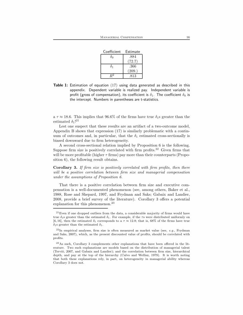
N+1 and V (w) = log(w). Data werecreated for 10,000 firms as follows. For each firm, its τ was a random draw fromthe Pareto distribution τ ∼ 1 − (6/τ)3 : [6,∞). Gabaix and Landier (2008)provide evidence for why a Pareto distribution reflects reality. Then, for eachfirm, the optimal contract was calculated, as was the N its manager wouldchoose in equilibrium. Whether that firm was successful or not was determinedby whether a uniformly distributed random variable on the unit interval wasless than P (N)—successful—or was above P (N)—failure. Once the data wereconstructed, equation (17) was estimated. The results are shown in Table 1.20

The estimated δ1, while estimated with great accuracy, is a poor measure ofactual incentives in this sample. For any given firm, the true coefficients solve

wf = δ0 + δ1 × 0 and ws = δ0 + δ1τ .

Hence a firm’s true δ1 is given by

δ1 =ws − wf

τ.

In the sample, the range of τ proved to be from 6.0010 to 132.32. The corre-sponding firm-specific δ1s are falling in τ from .670 to .147. This is considerablevariation. Moreover, the estimated cross-section δ1 is the true δ1 of a firm with

19Hermalin and Wallace also present reasons, different than those discussed here, for whythe δ1 estimated from (17) using cross-sectional data could be a biased-downward measure ofincentive strength.

20The Mathematica program used to generate the data is available from the author uponrequest.


Coefficient Estimateδ0 .884

(72.7)δ1 .366

(209.)R2 .813

Table 1: Estimation of equation (17) using data generated as described in thisappendix. Dependent variable is realized pay. Independent variable isprofit (gross of compensation), its coefficient is δ1. The coefficient δ0 isthe intercept. Numbers in parentheses are t-statistics.

a τ ≈ 18.6. This implies that 96.6% of the firms have true δ1s greater than theestimated δ1!

21

Lest one suspect that these results are an artifact of a two-outcome model,Appendix B shows that expression (17) is similarly problematic with a contin-uum of outcomes and, in particular, that the δ1 estimated cross-sectionally isbiased downward due to firm heterogeneity.

A second cross-sectional relation implied by Proposition 6 is the following.Suppose firm size is positively correlated with firm profits.22 Given firms thatwill be more profitable (higher τ firms) pay more than their counterparts (Propo-sition 6), the following result obtains.

Corollary 3. If firm size is positively correlated with firm profits, then therewill be a positive correlation between firm size and managerial compensationunder the assumptions of Proposition 6.

That there is a positive correlation between firm size and executive com-pensation is a well-documented phenomenon (see, among others, Baker et al.,1988, Rose and Shepard, 1997, and Frydman and Saks; Gabaix and Landier,2008, provide a brief survey of the literature). Corollary 3 offers a potentialexplanation for this phenomenon.23

21Even if one dropped outliers from the data, a considerable majority of firms would havetrue δ1s greater than the estimated δ1. For example, if the τs were distributed uniformly on[6, 16], then the estimated δ1 corresponds to a τ ≈ 12.8; that is, 68% of the firms have trueδ1s greater than the estimated δ1.

22In empirical analyses, firm size is often measured as market value (see, e.g., Frydmanand Saks, 2007), which, as the present discounted value of profits, should be correlated withprofits.

23As such, Corollary 3 complements other explanations that have been offered in the lit-erature. Two such explanations are models based on the distribution of managerial talent(Tervio, 2007, and Gabaix and Landier); and the correlation between firm size, hierarchicaldepth, and pay at the top of the hierarchy (Calvo and Wellisz, 1979). It is worth notingthat both these explanations rely, in part, on heterogeneity in managerial ability whereasCorollary 3 does not.

Alternative Formulations 17

The amount of firm resources, Y , is an alternative measure of size. Thefollowing proposition provides comparative statics when Y varies, but τ is fixed(to improve readability, τ is, thus, suppressed in the following).

Proposition 7. Assume firms don’t vary in type, but have different levels ofresources, Y . A manager of firm with a higher value of Y is paid at least as muchin expectation as a manager of a firm with a lower value of Y ; moreover, thereis an interval of Y , starting at 0, such that the manager’s expected compensationis strictly increasing with Y .

Proof: A firm’s profit can be written as

π = B(N(g)

)− C(g) . (18)

Because N(·) is strictly increasing, it is invertible and, hence, (18) can be rewrit-ten as

π = B(N) − c(N) , (19)

where c(N) = C(N−1(N)

). The firm’s objective is to maximize (19) with

respect to N subject to the boundary constraint N ≤ Y . For Y small, theconstraint binds, so relaxing it means a larger N , which in turn means a largerg, which in turn means higher expected compensation, C(g).

Corollary 4. Under the assumptions of Proposition 7, there is a positive cor-relation between firm size, measured as available resources (assets), and man-agerial compensation.

5 Alternative Formulations

5.1 Governance as a Multi-Dimensional Problem

There are multiple dimensions to governance. There is board structure, com-pensation, shareholder activism, and so forth. Heretofore, however, governancehas been treated as a scalar, g. In this section, the model is extended to allowgovernance to be a vector, g ∈ R

n+, n > 1.

Return to the model of Section 2 and let the manager’s utility be

u = S + v(Y − S,g) .

Assume that v(·, ·) continues to satisfy conditions (1)–(3), with g substitutedfor g. In lieu of (4), assume

v1j(·, ·) > 0 for all 1 < j < n ; (4′)

that is, an increase in any dimension of governance lowers the marginal benefitof diverting resources (equivalently, raises the marginal cost of doing so).

Lemma 1′. For all governance levels, g ∈ Rn+, there exists an amount Y (g),

such that, in equilibrium, the manager diverts a positive amount if and only if


total resources exceed Y (g) (i.e., iff Y > Y (g)). The equilibrium amount ofdiversion is S = max{Y − Y (g), 0}. Moreover, Y (·) is strictly increasing anddifferentiable in each argument (i.e., ∂Y/∂gj exists and is positive).

Assume v1(0,0) = 1, so Y (0) = 0.In lieu of (5), assume

∀x ∃g = (g1, . . . , gn) such that gj <∞ ∀j and v1(x,g) ≥ 1 . (5′)

Let the owners’ profits be

B(Y − S, τ) − C(g) ,

where the previous assumptions hold and C(·) is strictly increasing in each ofits arguments. Because increasing g along any dimension is costly, the ownerswill never choose a g such that Y (g) > Y . Define

G(Y ) ={g∣∣Y (g) ≤ Y

}.

In light of the assumption that v1(0,0) = 1, condition (5′), and the continuityof Y (·) as established by Lemma 1′, G(Y ) is compact. The owners problem is,thus,

maxg∈G(Y )

B(Y (g), τ

)− C(g) .

Because G(Y ) is compact and all functions are continuous, at least one solutionmust exist. Let g(τ) be the solution adopted by a type-τ firm.

The main comparative static result is the following:

Proposition 8. Higher-type firms spend at least as much on governance as dolower-type firms (i.e., if τ > τ ′, then C

(g(τ)

)≥ C

(g(τ ′)

)). Moreover, if a

lower-type firm has not blocked all resource diversion (i.e., Y(g(τ ′)

)< Y ), then

the higher-type firm spends strictly more (i.e., C(g(τ)

)> C

(g(τ ′)

)).

Recall the interpretation set forth in Section 2 that g be thought of as theexpenditure on governance; that is, g = C(g). In light of Proposition 8, one isfree to view the owners as solving a two-step process: first, for each y solve theproblem

ming

C(g) subject to Y (g) = y .

Let g(y) denote the solution. Then associate to each y a g ≡ C(g(y)); this yieldsa one-to-one strictly monotonic mapping. This mapping can be inverted to yielda function mapping g into y. By construction, that function is equivalent to theY (g) function used in Section 2. Observe, in this case, the cost of g is just g.24

A related question is whether higher-type firms employ stronger governanceon all dimensions than lower-type firms; that is, does τ > τ ′ imply g(τ) ≥ g(τ ′),

24To rule out corner solutions at no governance (i.e., g = 0) it was assumed in Section 2that C′(0) = 0. Under the interpretation here, C′(g) ≡ 1. Hence, an alternative solution isneeded to rule out solutions; one such assumption would be B1(0, τ) > 1 for all τ .


where the order over vectors is the usually piecewise ordering? It is readilyshown this implication cannot be true generally. For instance, suppose n = 2,v(Y − S,g) = v

(Y − S,max{g1, g2}

), and

C(g) = g1 +1

2g2 +

3

2

(

g2 − min

{

g2,2

3

})

,

then the optimal g to achieve effective governance level g = max{g1, g2} is (0, g)for g ≤ 1 and (g, 0) for g > 1. Hence, if g(τ ′) < 1 < g(τ), then g(τ ′) and g(τ)cannot be compared (i.e., neither g(τ) ≥ g(τ ′) nor g(τ ′) ≥ g(τ) are true).

In the preceding example, the two dimensions of governance are perfect sub-stitutes. If the dimensions of governance are complements, then the desiredimplication, τ > τ ′ ⇒ g(τ) ≥ g(τ ′), follows from Topkis’s Monotonicity Theo-rem (Milgrom and Roberts, 1990, p. 1262):

Proposition 9. Suppose that the manager’s marginal benefit from behaving ina manner desired by the owners, v1(y,g), exhibits complementarities in gov-ernance; specifically, assume it is supermodular in g. Suppose it also exhibitsincreasing differences; that is, if y > y′ and g ≥ g′, then

v1(y,g) − v1(y′,g) > v1(y,g

′) − v1(y′,g′) .

Finally suppose that the marginal cost of governance in one dimension is non-increasing in any other dimension (i.e., ∂2C(g)/(∂gi∂gj) ≤ 0, i 6= j).25 Thenthe governance of a higher-type firm on any given dimension is no less than thatof a lower-type firm on that dimension; that is, τ > τ ′ implies g(τ) ≥ g(τ ′).

Observe that if (i) v(y,g) has the form

v(y,g) = γ(g)υ(y) (20)

plus, possibly, additional terms with zero cross-partial derivatives in gi and yfor all i; if (ii) γ(·) is increasing in its arguments, with positive cross-partialderivatives; and if (iii) υ(·) is increasing, then the conditions on v1(y,g) setforth in Proposition 9 all hold. Observe further that (20) has the followinginterpretation: given a choice of g, the firm has an “effective” level of governanceγ(g).26 The owners’ problem can, thus, be seen as choosing, for each effectivelevel of governance γ, the cost-minimizing vector g(γ). The cost of such aneffective level is C

(g(γ)

)≡ C(γ). Viewing γ as the equivalent of g in Sections 2

25Observe this condition would hold if C(g) were additive across the dimensions; that is, if

C(g) =n

X

i=1

ci(gi) , .

where ci(·) is strictly increasing for all i.

26The effective level of governance is increasing in each dimension of governance and themarginal effective level in any one dimension is increasing in any other dimension (e.g., γ(·)exhibits complementarities).


and 3, the analysis in those earlier sections can be seen as short-hand for a moreelaborate model in which the owners set governance on many dimensions in acost-minimizing way to achieve an effective level of governance (the g in thosesections).

Whether different dimensions of governance are complements or substitutesis an empirical question. This question does not seem to have attracted muchattention. A partial exception is Hermalin and Wallace (2001), which studies,inter alia, whether firms base incentive compensation on the same measuresor different measures. They find evidence that if a firm heavily weights onemeasure, it will tend not to weight another; whereas if a firm heavily weightsthe other, it will tend not to weight the one. With respect to compensation,these findings support a view that dimensions of governance are substitutes.On the other hand, they neglect many other dimensions, so the overall issue ofcomplements versus substitutes must be seen as open.

5.2 Heterogeneity in Cost of Governance

An alternative to assuming heterogeneity in the benefit function, B(·, ·), is to as-sume heterogeneity in the cost-of-governance function. To explore this, considerthe model of Section 2, except write the owners’ payoff as B(Y − S) − C(g, θ),where θ denotes firm type in this alternative specification. As a definition oftype, assume

C12(·, ·) < 0 ; (6′)

that is, higher-type firms have lower marginal costs of governance. A straight-forward modification of the proof of Proposition 1 shows that

Proposition 1′. In a heterogeneous costs model, higher-type firms adopt atleast as great a level of governance as lower-type firms (i.e., if θ > θ′, theng(θ) ≥ g(θ′)). Moreover, if a lower-type firm has not adopted the maximumlevel of governance (i.e., g(θ′) < g),27 then a higher-type firm will have a strictlygreater level of governance (i.e., g(θ) > g(θ′)).

If C2(0, θ) ≤ 0 for all θ, then it also follows that

Proposition 2′. Under the assumptions of the heterogenous costs model andassuming a common level of resources, Y , a firm that will be more profitable inequilibrium than another has at least as high a level of governance as the otherfirm.

and

Proposition 4′. Assuming (6 ′) and endogenous investment, there will be astrictly positive correlation between the amount the owners invest in a firm andits level of governance. Furthermore, if governance cost is decreasing in firmtype (i.e., C2(g, θ) < 0), then there will be a strictly positive, but non-causal,correlation between firm profit and level of governance.

27Recall g is the solution to Y (g) = Y .

Trends in Governance 21

In short, the model operates the same whether it is assumed that hetero-geneity stems from different profit potentials or it is assumed that heterogeneitystems from different marginal costs of governance across firms.

There are numerous reasons firms could have different marginal costs ofachieving a given level of effective governance (i.e., a level that deters a givenamount of agency behavior). Monitoring in some settings could be more difficultthan in others (Demsetz and Lehn, 1985, among others make this point). Forexample, it could be more difficult to determine what is going on with firmsin fast-changing or highly innovative industries than with firms in staid andpredictable industries. Or for instance, it could be more difficult to monitora conglomerate operating in many industries than a firm operating in a singleindustry. Variation in laws and regulations across time or place could lead todifferences in governance costs across time or space.

Although there is no reason to think that heterogeneity is solely on thebenefit or cost side, one might ask which is more relevant. This is, obviously,an empirical question. One piece of evidence that points to the benefit sideis the trend towards increased use of outside directors on the board in theUnited States and other countries over the past quarter decade or more (see,for instance, Borokhovich et al., 1996, Dahya et al., 2002, and Huson et al.,2001). It is difficult to see this trend as reflecting a drop in the marginal costof outside directors. If anything, the evidence suggests the marginal cost ofoutside directors has increased; certainly, outside director compensation hasincreased (see, e.g., Huson et al.). Another piece of evidence is the increasedpayout to executives, particularly from incentive pay (Hall and Liebman report anearly seven-fold increase in the amount of options granted managers from 1980to 1994). It is unclear what, if anything, has changed over the past thirty yearsto make the marginal cost of incentive pay decrease.

6 Trends in Governance

There have been numerous trends in corporate governance over the past twentyto thirty years (see, e.g., Becht et al. and Holmstrom and Kaplan, 2001, forsurveys). As noted above, the proportion of outside directors on boards hassteadily increased in the United States and other countries (Borokhovich et al.;Dahya et al.; and Huson et al.). There has been growing use of stock-basedincentives for directors over the period 1989 to 1997 (Huson et al.). Kaplan andMinton (2006) find evidence that ceo turnover rates in the period 1998–2005 aresignificantly greater than in the period 1992–1998; and the rate in that periodis greater than found in studies for the pre-1992 period. They interpret thisas evidence of better monitoring by boards of directors. Consistent with thisinterpretation is the finding of Huson et al. that firings, as a percentage of allceo successions, were trending upward in the period 1971 to 1994. These trendscan all be interpreted as evidence that governance has been getting stronger overthe past twenty to thirty years.

At the same time, there is evidence that firms’ profit potential and resourceshave been increasing during this period. As Gabaix and Landier note, there

Conclusions 22

has been a six-fold increase in the market value of the top 500 us firms be-tween 1980 and 2003. From 1973 to 2003, there has been a three-fold increasein patents granted in the us; and, since the late 1980s, evidence of increasedproductivity in r&d (Hall, 2004). Technological progress has been remarkablein this period, especially with respect to information technology and telecom-munications. Since the mid-1990s, there has been a growth in productivity thathas not resulted in a significant increase in wages (DeLong, 2003).

The analysis in Sections 2–4 offers a way of tying these two trends to-gether. As the potential profitability and resources of firms increased, the valueof improved governance also rose. Consequently, governance got stronger (onaverage—the model does not predict any kind of convergence across firms).

This is not to say the process was necessarily smooth. As noted by manyauthors, one might expect management to resist improved governance. This re-sistance could have led to more aggressive forms of change, such as the takeovers,leveraged buyouts, and proxy fights that characterized the 1980s. It could alsohave motivated shareholders to seek change through legislation or changes in thelisting requirements of exchanges. But over time, as suggested by Holmstromand Kaplan, a new equilibrium with stronger governance has emerged.

Tying the change in governance to changes in the resources and potential offirms also serves to explain why changes in governance occurred when they did.After all, commentators have been complaining about the state of governancefor a long time (consider, e.g., Berle and Means, 1932), so presumably somethinghad to occur to motivate action. Until the point that the payoff from improvedgovernance made imposing it worthwhile, investors were not willing to walk thetalk.

The model set forth above offers a broader explanation for change than thatset forth by Tervio or Gabaix and Landier, which are concerned with executivecompensation only; moreover, their models suggest a relatively smooth processin which growth in firm size increases executive compensation.28 Like the modelhere, Hermalin (2005) offers an explanation for improvements, broadly, in gov-ernance, but his explanation is based on the rise of institutional investors.29

His explanation can be seen as complementary to the one set forth here insofaras greater institutional holding could reduce the free-riding problem among eq-uity holders with respect to taking action; hence, greater institutional holdingcould serve to reduce the owners’ marginal cost of governance, which, follow-ing Proposition 1′, would yield higher levels of governance. Alternatively, anincrease in holdings by institutional investors can be seen as a rise in τ—as alarger proportion of profits accrue to these investors, their incentive to push forstronger governance increases.

28Another explanation primarily focused on executive compensation is the model of Murphyand Zabojnık (2003), which argues that changes in the ceo labor market, specifically a greateremphasis on general versus firm-specific knowledge, explains the rise in ceo compensation.

29Huson et al. report that the percentage of us equity held by institutional investors hasincreased from 20% in 1971 to 45% in 1994. Gompers and Metrick (2001) report a similardoubling from 1980 to 1996.

Conclusions 23

7 Conclusions

This paper has sought to make the case that firms are not profitable becausethey have good corporate governance, rather they have good corporate gover-nance because they are profitable. This is not to say, of course, that corporategovernance is irrelevant, but instead to say that the observed variation in gov-ernance across firms is not the cause of observed variation in their profits.

This insight holds important implications for empirical work in corporategovernance and, to an extent, in the study of organizations generally. Theendogenous characteristics of an organization are, presumably, chosen to facili-tate the organization’s objectives. If organizations are behaving optimally, thenvariation in how well they do cannot be explained by variation in their char-acteristics. However, as shown here, the variation in their characteristics couldwell be a tied to variation in the potentials they have to do well.

To be sure, real-life optimizing is often a trial-and-error process. Hence,at any moment in time, organizations could be making errors and, thus, somevariation in chosen characteristics is explaining some of the variation in perfor-mance. But if the variation in characteristics persists over time, then the weightone can place on cross-sectional regressions’ representing evidence of causationis de minimus.

What might these insights hold for empirical work? One course suggestedby this paper is to consider exogenous firm attributes that plausibly predictprofitability and see whether they predict patterns in governance (somewhatanalogous to earlier work that looks for attributes that plausibly predict thecosts of ameliorating agency problems and their ability to predict patterns ingovernance). A second course is, for some aspects of governance such as com-pensation, to make greater use of panel data and employ random-coefficient orsimilar models to estimate firm-specific coefficients. For instance, in the pay-for-performance regression (17), estimate the coefficients δ0 and δ1 on a firm-by-firmbasis.30 A third course is to examine the consequences of regulated changes thatare binding on some firms (e.g., those resulting from the Sarbanes-Oxley Act).If firms were optimizing prior to the regulated change, then those firms for whichthe regulations are binding should suffer poorer performance subsequent to theregulations than firms for which the regulations were not binding (i.e., thanfirms that were meeting the regulations prior to their enactment).

Beyond empirical work, future research may wish to model the dynamics ofgovernance change. Although some sense of how the model might be extendedto a dynamic setting was given in Section 6, this is far from a complete analysis.Moreover, in a dynamic setting, many models presume managers can entrenchthemselves or otherwise gain influence over how they are governed (surveysby Becht et al. and Hermalin and Weisbach discuss such models). In termsof the model presented above, this suggests that the cost of governance (i.e.,C(g)) could rise over time if the same management team remains in office.

30Hermalin and Wallace essentially employ this approach in their study of pay for perfor-mance; they find evidence for a much stronger pay-for-performance relationship using thisapproach than suggested by a cross-sectional analysis of the same data.

Conclusions 24

Particularly if the marginal cost increases, then governance strength will declineand, consequently, so will profits.

To an extent, entrenchment and managerial influence are, themselves, aproduct of the initial governance system, which suggests that, when a dynamicperspective is taken, initial governance might be overly strong when viewed atthat point in time, but is optimal vis-a-vis the dynamic game. Other factorsthat influence the play of a dynamic game would be adjustment costs related togovernance. In short, numerous issues will arise when this analysis is extended toa dynamic framework. Nonetheless, the basic messages of the paper concerningcausality and the importance of firm heterogeneity are unlikely to be overturnedby such an extension.


Appendix A: Proofs

Proof of Lemma 1: Fix a g. From (3) and the continuity and monotonicityof v1(·, g), there exists a Y (g) <∞ such that

v1(Y (g), g

)= 1 . (21)

The manager’s problem is

maxS≥0

S + v(Y − S, g) . (22)

The derivative = 1 − v1(Y − S, g)

{< 0 , if Y − S < Y (g)> 0 , if Y − S > Y (g)

,

where the inequalities follow from (21) because (22) is strictly concave. It fol-lows the manager does best to set S = 0 if Y < Y (g) and S > 0 if Y > Y (g).In the latter case, it is readily seen the manager’s optimal S = Y − Y (g). Themoreover part follows because raising g increases the left-hand side of (21) by(4), hence, by concavity, Y (g) must increase to restore equality. That Y (·) isdifferentiable follows from the implicit function theorem.

Proof of Lemma 2: By the definition of an optimum (revealed preference):

f(x, z) ≥ f(x′, z) and (23)

f(x′, z′) ≥ f(x, z′) . (24)

Expressions (23) and (24) imply

0 ≤(f(x, z) − f(x′, z)

)−

(f(x, z′) − f(x′, z′)

)

=

∫ x

x′

(f1(x, z) − f1(x, z

′))dx =

∫ x

x′

(∫ z

z′

f12(x, ζ)dζ

)

dx ,

where the integrals follow from the fundamental theorem of calculus. The innerintegral in the rightmost term is positive because f12(·, ·) > 0 and the directionof integration is left to right. It follows that the direction of integration in theouter integral must be weakly left to right; that is, x′ ≤ x. To establish themoreover part, because f1(·, ζ) is a differentiable function for all ζ, if x′ is aninterior maximum, then it must satisfy the first-order condition

0 = f1(x′, z′) .

Because f12(·, ·) > 0 implies f1(x′, z) > f1(x

′, z′), it follows that x′ does notsatisfy the necessary first-order condition for maximizing f1(x, z). Thereforex′ 6= x; so, by the first half of the lemma, x′ < x.

Proof of Lemma 3: Given that N(·) is increasing, it is sufficient to showthat the standard agency problem of implementing N at minimum cost yieldsa cost function c(N) that is increasing in N . The standard problem is

min{vs,vf}

P (N)V −1(vs) +(1 − P (N)

)V −1(vf ) (p)


subject to

P ′(N)(vs − vf ) − 1 = 0 and (ic)

P (N)vs +(1 − P (N)

)vf ≥ 0 . (ir)

The solution is readily shown to be

vf = − P (N)

P ′(N)and vs =

1 − P (N)

P ′(N).

Hence,

c(N) = P (N)V −1

(1 − P (N)

P ′(N)

)

+(1 − P (N)

)V −1

(

− P (N)

P ′(N)

)

.

Observe that c(N) is the expected value of a convex function over a two-pointdistribution that has a mean of zero for all N ; that is,

P (N)vs +(1 − P (N)

)vf =

P (N)(1 − P (N)

)

P ′(N)− P (N)

(1 − P (N)

)

P ′(N)= 0 .

Because the left point of the distribution is falling in N (i.e., dvf/dN < 0) andthe right point is increasing in N (i.e., dvs/dN > 0), an increase in N representsa mean-preserving spread. From Jensen’s inequality, it follows that c(N) mustbe increasing in N .

Proof of Lemma 1′: The proof up to the “moreover” part mimics that ofLemma 1 and is omitted for the sake of brevity. The moreover part follows be-cause raising any element of g increases the left-hand side of (21) by (4′), hence,by concavity, Y (g) must increase to restore equality. That Y (·) is differentiablefollows from the implicit function theorem.

Proof of Proposition 8: Let τ > τ ′. To reduce notational clutter, letg = g(τ) and g′ = g(τ ′). To prove the first part of the proposition it is sufficientto show that Y (g) ≥ Y (g′); because, if Y (g) ≥ Y (g′) but C(g) < C(g′), thenthe τ ′-type firm cannot be optimizing—it could weakly increase its benefit andstrictly lower its costs by switching to g. By revealed preference:

B(Y (g), τ

)− C(g) ≥ B

(Y (g′), τ

)− C(g′) and (25)

B(Y (g′), τ ′

)− C(g′) ≥ B

(Y (g), τ ′

)− C(g) . (26)

Expressions (25) and (26) can be combined to yield

B(Y (g), τ

)−B

(Y (g′), τ

)≥ B

(Y (g), τ ′

)−B

(Y (g′), τ ′

).

Twice applying the fundamental theorem of calculus, this last expression canbe rewritten as

∫ τ

τ ′

∫ Y (g)

Y (g′)

B12(y, t)dydt ≥ 0 . (27)


Because B12(·, ·) > 0 and τ > τ ′, (27) can be non-negative only if the directionof integration for the inner integral is left to right; that is, only if Y (g) ≥ Y (g′).As noted, this implies C(g) ≥ C(g′), as was to be shown.

Turning to the moreover part, the goal is to show Y (g) > Y (g′). Suppose,instead, that Y (g) = Y (g′). One of the types would, therefore, have to beplaying non-optimally if C(g) 6= C(g′); hence, this supposition implies C(g) =C(g′). The τ ′-type firm is at an interior solution, so there must be at least oneg′j such that

B1

(Y (g′), τ ′

)Yj(g

′) − Cj(g′) = 0 .

Because B12(·, ·) > 0, this implies

B1

(Y (g′), τ

)Yj(g

′) − Cj(g′) > 0 .

It follows there exists a governance vector g that has slightly more on the jthdimension such that

B(Y (g), τ

)− C(g) > B

(Y (g′), τ

)− C(g′) = B

(Y (g), τ

)− C(g) ,

where the equality follows because Y (g) = Y (g′) and C(g) = C(g′). Butthen, g was not optimal for the τ -type firm, a contradiction. By contradic-tion, Y (g) 6= Y (g′), which, given the first part of the proposition, entailsY (g) > Y (g′). It must then be that C(g) > C(g′) because otherwise theτ ′-type firm is not behaving optimally.

Proof of Proposition 9: In light of Proposition 8, define

C(y) = ming∈G(Y )

C(g) subject to y = Y (g) . (28)

The cost, C(g), is increasing in each dimension and so is Y (g) (the latter followsfrom Lemma 1′). Consequently, C(·) is an increasing function. The owners’problem can be reexpressed as

maxy≤Y

B(y, τ) − C(y) . (29)

Let y(τ) be the solution to (29) selected by a type-τ firm. Utilizing Lemma 2,it is readily shown that τ > τ ′ implies y(τ) ≥ y(τ ′). The proposition follows ifit can be shown that y(τ) ≥ y(τ ′) implies g(τ) ≥ g(τ ′).

To that end, observe that minimization program in (28) is equivalent to theprogram

maxg∈G(Y )

−C(g) subject to (30)

v1(y,g) = 1 (31)

Let λ be the Lagrange multiplier on (31). The program given by (30) is, thus,equivalent to

maxg,λ

−C(g) + λ(v1(y,g) − 1

). (32)

Appendix B: Issues in the Estimation of the Pay-for-Performance Relation 28

This expression is supermodular in (g, λ) in light of Topkis’s characterizationtheorem (Milgrom and Roberts, 1990, p. 1261) because v1i(y,g) > 0 by (4′) andv1ij(y,g) ≥ 0 and −Cij(g) ≥ 0 by the assumptions of the proposition.31 Bythe increasing-differences assumption of the proposition, (32) exhibits increas-ing differences in y and gi for any i. Let g(y) denote the solution to (32). Itfollows, therefore, from Topkis’s monotonicity theorem (Milgrom and Roberts,p. 1262) that y > y′ implies the g(y) ≥ g(y′).

Appendix B: Issues in the Estimation of the Pay-for-

Performance Relation

Consider the following agency model. The manager’s utility is

−1

exp(Y −N︸︷︷︸

S

+δ0 + δ1π) ,

where his compensation contract is δ0 + δ1π, π being realized profits gross ofcompensation. Assume that32

π ∼ N(τ log(N), σ2

),

In what follows, assume Y is sufficiently large that the constraint N ≤ Y neverbinds.

Using the formula for the moment-generating function of a normal randomvariable, the manager’s expected utility is

−1

exp(Y −N + δ0 + δ1τ log(N) − 1

2δ21σ

2) .

A monotonic transformation is

Y −N + δ0 + δ1τ log(N) − 1

2δ21σ

2 . (33)

Given δ0 and δ1, the manager maximizes (33) with respect to N . This yields

N = δ1τ .

31v1ij denotes the third partial derivative of v with respect to y, gi, and gj .

32Note the assumed compensation contract is not second-best optimal under these assump-tions (see Mirrlees, 1974). A reformulation of this simple model along the lines of Holmstromand Milgrom (1987)—in particular, assuming the manager decides how much to divert on acontinuous basis with the resulting net funds controlling the drift of a Brownian motion—would, however, yield an optimal compensation contract of this form. One can thus view themodel here as a simple approximation of that more complex model. In any case, given theissue is the econometric consequences of heterogeneity, the optimality of the contract is notessential to the analysis.


Hence, if the owners want to induce a particular N , they must set δ1 to satisfy

δ1 =N

τ. (34)

Assume, as an alternative to working for the firm, the manager could get a jobthat paid a flat wage of w. Hence, the owners must set δ0 to satisfy

Y −N + δ0 +N

τ︸︷︷︸

δ1

τ log(N) − 1

2

N2

τ2︸︷︷︸

δ2

1

σ2 ≥ w .

Given the owners’ profit is decreasing in δ0, the constraint will bind and, thus,

δ0 = w − Y +N −N log(N) +1

2N2 σ

2

τ2. (35)

The owners seek to choose N to maximize their expected profits. Using (34)and (35), their expected profits can be written as

τ log(N) − w + Y −N − 1

2N2 σ

2

τ2.

The first-order condition is

τ

N− 1 −N

σ2

τ2= 0 .

Solving for the root that satisfies the second-order condition yields

N =τ3/2

√4σ2 + τ − τ2

2σ2. (36)

Plugging (36) into (34) and (35) yields expressions for δ1 and δ0, respectively,in terms of the model’s primitives (τ , σ2, Y , and w).

Data were created for 10,000 firms as follows. For each firm, its τ was arandom draw from the uniform distribution τ ∼ U : [10, 20]. To insure thatN ≤ Y was never binding, Y = 400. The reservation wage, w, was set tozero. Then, for each firm, the optimal contract was calculated, as was the N itsmanager would choose in equilibrium. Profits gross of compensation, π, werethen generated for that firm as a draw from N (τ log(N), 1) and the resultingcompensation for the manager calculated. Once the data were constructed,equation (17) was estimated with π as the independent variable. The resultsare shown in Table 2.33

The true δ1s for firms with τ ∈ [10, 20] ranges from [.916, .954]; hence, theestimate δ1 is less than the true δ1 for 100% of the firms. The reason why

33The Mathematica program used to generate the data is available from the author uponrequest.


Coefficient Estimateδ0 -396.46

(-15321.)δ1 .27568

(440.69)R2 .95104

Table 2: Estimation of equation (17) using data generated as described in thisappendix. Dependent variable is realized pay. Independent variable isprofit (gross of compensation), its coefficient is δ1. The coefficient δ0 isthe intercept. Numbers in parentheses are t-statistics.

(17) does so poorly is that while the true δ1s are fairly constant across τ , theintercepts—the true δ0s—vary considerably. Because low τ firms have greaterδ0s and tend to have lower πs, while high τ firms have lower δ0s and tendto have higher πs, the estimated slope between pay and profits is flattened.Consequently, the estimated δ1 is biased downward.

References 31

References

Baker, George P., Michael C. Jensen, and Kevin J. Murphy, “Com-pensation and Incentives: Practice vs. Theory,” Journal of Finance, 1988, 43(3), 593–616.

Becht, Marco, Patrick Bolton, and Ailsa Roell, “Corporate Governanceand Control,” in George Constantinides, Milton Harris, and Rene Stulz, eds.,The Handbook of the Economics of Finance, Amsterdam: North-Holland,2003.

Berger, Philip G., Eli Ofek, and David L. Yermack, “Managerial En-trenchment and Capital Structure Decisions,” Journal of Finance, September1997, 52 (4), 1411–1438.

Berle, Adolph A. and Gardiner C. Means, The Modern Corporation andPrivate Property, New York: MacMillan, 1932.

Bhagat, Sanjai and Richard H. Jefferis, The Econometrics of CorporateGovernance Studies, Cambridge, MA: MIT Press, 2002.

Borokhovich, Kenneth A., Robert P. Parrino, and Teresa Trapani,“Outside Directors and CEO Selection,” Journal of Financial and Quantita-tive Analysis, September 1996, 31 (3), 337–355.

Calvo, Guillermo A. and Stanislaw Wellisz, “Hierarchy, Ability, and In-come Distribution,” Journal of Political Economy, October 1979, 87 (5, Part1), 991–1010.

Coles, Jeffrey L., Michael L. Lemmon, and J. Felix Meschke, “Struc-tural Models and Endogeneity in Corporate Finance: The Link Between Man-agerial Ownership and Corporate Finance,” 2007. Working Paper, ArizonaState University.

Dahya, Jay, John J. McConnell, and Nickolaos G. Travlos, “The Cad-bury Committee, Corporate Performance, and Top Management Turnover,”Journal of Finance, 2002, 57 (1), 461–483.

DeLong, J. Bradford, “Productivity Growth in the 2000s,” in Mark Gertlerand Kenneth Rogoff, eds., NBER Macroeconomics Annual 2002, Cambridge,MA: MIT Press, 2003.

Demsetz, Harold and Kenneth Lehn, “The Structure of Corporate Own-ership: Causes and Consequences,” Journal of Political Economy, December1985, 93 (6), 1155–1177.

Frydman, Carola and Raven E. Saks, “Executive Compensation: A NewView from a Long-Term Perspective, 1936–2005,” July 2007. Unpublishedworking paper, MIT Sloan.

References 32

Gabaix, Xavier and Augustin Landier, “Why Has CEO Pay Increased SoMuch?,” Quarterly Journal of Economics, 2008, 123 (1), 49–100.

Gompers, Paul A. and Andrew Metrick, “Institutional Investors and Eq-uity Prices,” Quarterly Journal of Economics, February 2001, 116 (1), 229–259.

Grossman, Sanford J. and Oliver D. Hart, “Corporate Financial Struc-ture and Managerial Incentives,” in John J. McCall, ed., The Economics ofInformation and Uncertainty, University of Chicago, 1982.

and , “An Analysis of the Principal-Agent Problem,” Econometrica, 1983,51, 7–46.

Hall, Brian J. and Jeffrey B. Liebman, “Are CEOs Really Paid Like Bu-reaucrats?,” Quarterly Journal of Economics, August 1998, CXIII (3), 653–691.

Hall, Bronwyn H., “Exploring the Patent Explosion,” Journal of TechnologyTransfer, December 2004, 30 (1–2), 35–48.

Harris, Milton and Artur Raviv, “Corporate Control Contests and CapitalStructure,” Journal of Financial Economics, 1988, 20, 55–86.

Hart, Oliver D. and John H. Moore, “Default and Renegotiation: A Dy-namic Model of Debt,” Quarterly Journal of Economics, February 1998, 113(1), 1–41.

Haubrich, Joseph G., “Risk Aversion, Performance Pay, and the Principal-Agent Problem,” Journal of Political Economy, April 1994, 102 (2), 258–276.

Hermalin, Benjamin E., “Heterogeneity in Organizational Form: WhyOtherwise Identical Firms Choose Different Incentives for their Managers,”RAND Journal of Economics, Winter 1994, 25 (4), 518–537.

, “Trends in Corporate Governance,” Journal of Finance, 2005, 60 (5), 2351–2384.

and Michael S. Weisbach, “Boards of Directors as an Endogenously De-termined Institution: A Survey of the Economic Literature,” Economic PolicyReview, April 2003, 9 (1), 7–26.

and Nancy E. Wallace, “Firm Performance and Executive Compensationin the Savings and Loan Industry,” Journal of Financial Economics, 2001,61, 139–170.

Himmelberg, Charles P., R. Glenn Hubbard, and Darius Palia, “Un-derstanding the Determinants of Managerial Ownership and the Link betweenOwnership and Performance,” Journal of Financial Economics, September1999, 53 (3), 353–384.

References 33

Holmstrom, Bengt and Paul Milgrom, “Aggregation and Linearity in theProvision of Intertemporal Incentives,” Econometrica, March 1987, 55 (2),303–328.

and Steven N. Kaplan, “Corporate Governance and Merger Activity in theUnited States: Making Sense of the 1980s and 1990s,” Journal of EconomicPerspectives, Spring 2001, 15 (2), 121–144.

Huson, Mark R., Robert Parrino, and Laura T. Starks, “Internal Mon-itoring Mechanisms and CEO Turnover: A Long-Term Perspective,” Journalof Finance, December 2001, 55 (6), 2265–2297.

Jensen, Michael C., “Agency Costs of Free Cash Flow, Corporate Finance,and Takeovers,” American Economic Review, May 1986, 76 (2), 323–329.Papers and Proceedings of the Ninety-Eighth Annual Meeting of the AmericanEconomic Association.

and Kevin J. Murphy, “Performance Pay and Top-Management Incen-tives,” Journal of Political Economy, 1990, 98, 225–264.

and William H. Meckling, “Theory of the Firm: Managerial Behavior,Agency Costs, and Capital Structure,” Journal of Financial Economics, 1976,3, 305–360.

Kaplan, Steven N. and Bernadette A. Minton, “How has CEO TurnoverChanged? Increasingly Performance Sensitive Boards and Increasingly Un-easy CEOs,” July 2006. Unpublished working paper, University of ChicagoGSB.

Milgrom, Paul and John Roberts, “Rationalizability, Learning, and Equi-librium in Games with Strategic Complementarities,” Econometrica, 1990,58, 1255–1277.

Mirrlees, James, “Notes on Welfare Economics, Information, and Uncer-tainty,” in Michael S. Balch, Daniel L. McFadden, and Shih-Yen Wu, eds., Es-says on Economic Behavior Under Uncertainty, Amsterdam: North-Holland,1974.

Modigliani, Franco and Merton H. Miller, “The Cost of Capital, Corpo-rate Finance, and the Theory of Corporation Finance,” American EconomicReview, 1958, 48, 261–297.

Murphy, Kevin J. and Jan Zabojnık, “Managerial Capital and the Marketfor CEOs,” December 2003. Marshall School of Business Working Paper,University of Southern California.

Palia, Darius, “The Endogeneity of Managerial Compensation in Firm Value:A Solution,” Review of Financial Studies, Autumn 2001, 14 (3), 735–764.

References 34

Rose, Nancy L. and Andrea Shepard, “Firm Diversification and CEO Com-pensation: Managerial Ability or Executive Entrenchment?,” RAND Journalof Economics, Autumn 1997, 28 (3), 489–514.

Smith, Adam, An Inquiry into the Nature and Causes of the Wealth of Na-tions, Indianapolis: Liberty Press, 1776.

Stulz, Rene M., “Managerial Control of Voting Rights : Financing Policiesand the Market for Corporate Control,” Journal of Financial Economics,1988, 20, 25–54.

Tervio, Marko, “The Difference That CEOs Make: An Assignment Model Ap-proach,” February 2007. Unpublished working paper, University of California,Berkeley.

Firm Value and Corporate Governance -...

Documents

Transcript of Firm Value and Corporate Governance -...