Finite Strain Behavior of Polyureafor a Wide Range of Strain Rates

by

Jongmin Shim

M.S., Massachusetts Institute of Technology (2005)M.S., Korea Advanced Institute of Science of Technology (2001)B.S., Korea Advanced Institute of Science of Technology (1998)

Submitted to the Department of Civil and Environmental Engineeringin partial fulfillment of the requirements for the degree of

Doctor of Philosophy in the field of Engineering Mechanics

at the

MASSACHUSETTS INSTITUTE OF TECHNOLOGY

February 2010

c° 2009 Massachusetts Institute of Technology. All rights reserved.

Signature of Author . . . . . . . . . . . . . . . . . . . . . . . . . . . . . . . . . . . . . . . . . . . . . . . . . . . . . . . . . . . . . . . . . . .Department of Civil and Environmental Engineering

November 16, 2009

Certified by . . . . . . . . . . . . . . . . . . . . . . . . . . . . . . . . . . . . . . . . . . . . . . . . . . . . . . . . . . . . . . . . . . . . . . . . . . .Tomasz Wierzbicki

Professor of Applied Mechanics, Department of Mechanical EngineeringThesis Supervisor

Certified by . . . . . . . . . . . . . . . . . . . . . . . . . . . . . . . . . . . . . . . . . . . . . . . . . . . . . . . . . . . . . . . . . . . . . . . . . . .Dirk Mohr

CNRS Assistant Research Professor, École PolytechniqueThesis Supervisor

Certified by . . . . . . . . . . . . . . . . . . . . . . . . . . . . . . . . . . . . . . . . . . . . . . . . . . . . . . . . . . . . . . . . . . . . . . . . . . .Eduardo Kausel

Professor of Civil and Environmental EngineeringThesis Reader

Accepted by. . . . . . . . . . . . . . . . . . . . . . . . . . . . . . . . . . . . . . . . . . . . . . . . . . . . . . . . . . . . . . . . . . . . . . . . . . .Daniele Veneziano

Chairman, Departmental Committee for Graduate Students

Finite Strain Behavior of Polyurea

for a Wide Range of Strain Rates

by

Jongmin Shim

Submitted to the Department of Civil and Environmental Engineeringon November 16, 2009, in partial fulfillment of the

requirements for the degree ofDoctor of Philosophy in the field of Engineering Mechanics

Abstract

Polyurea is a special type of elastomer that features fast setting time as well as good chemicaland fire resistance. It has also good mechanical properties such as its high toughness-to-densityratio and high strain rate-sensitivity, so its application is recently extended to structural purposeto form sandwich-type or multi-layered plates. Those structures can be used for retrofitting ofmilitary vehicles and historic buildings, absorbing energy during structural crash.

In order to investigate its behavior of hysteresis as well as rate-sensitivity, three differenttesting systems are used to cover a wide range of strain rates up to strain of 100%. In viewof impact and blast events, the virgin state of polyurea is considered throughout the exper-iments. First, a hydraulic universal testing machine is used to perform uniaxial compressiveloading/unloading tests in order to investigate its hysteresis behavior at low strain rates (0.001/sto 10/s). Second, two distinct gas-gun split Hopkinson pressure bar [SHPB] systems are em-ployed to cover high strain rates: a nylon bar system (700/s to 1200/s) and an aluminum barsystem (2300/s to 3700/s). Lastly, the rate-sensitivity for intermediate strain rates (10/s to1000/s) is characterized using a modified SHPB system. The device is composed of a hydraulicpiston along with nylon input and output bars.

A finite strain constitutive model of polyurea is presented in order to predict the hysteresisand rate-sensitivity behavior. The 1-D rheological concept of two Maxwell elements in parallelis employed within the framework of the multiplicative decomposition of the deformation gra-dient. Model parameters are calibrated based on the uniaxial compressive tests at various rates.The corresponding algorithms is implemented as a user-defined material subroutine VUMATfor ABAQUS/Explicit, and used to predict the response of polyurea. The proposed consti-tutive model reasonably captures the experimentally observed asymmetric rate-sensitivity andstress-relaxation behavior: strong rate-sensitivity and large amount of stress relaxation dur-ing loading phase, but weak rate-sensitivity and smaller amount of stress relaxation duringunloading phase. In order to validate the proposed model, various dynamic punching testsare performed, and their results are well compared with the model predictions during loadingalthough the prediction of unloading behavior can be further improved.

Thesis Supervisor: Tomasz WierzbickiTitle: Professor of Applied Mechanics, Department of Mechanical Engineering

2

Thesis Supervisor: Dirk MohrTitle: CNRS Assistant Research Professor, École Polytechnique

Thesis Reader: Eduardo KauselTitle: Professor of Civil and Environmental Engineering

3

Acknowledgments

I would like to express my deep gratitude to Professor Tomasz Wierzbicki for taking me into the

Impact and Crashworthiness Lab and providing me with much needed support, guidance, and

mentorship. He has enlightened me on how important to keep an engineering mind. My sincere

thanks are due Professor Dirk Mohr at École Polytechnique for his mentorship and his valuable

insight into my research. He has shown me an excellent example for how to do research. I would

also like to offer many thanks to Professor Eduardo Kausel, Professor Jerome J. Connor, and

Professor David Roylance for their participation in my thesis committee and for their helpful

comments. Moreover, I am indebted to Professor Gerard Gary at École Polytechnique for his

guidance into the split Hopkinson pressure systems. The financial support of this work through

the Office of Naval Research is also greatly acknowledged.

I would like to thank all the members and alumni of the ICL (Dr. Young-Woong Lee, Dr.

Xiaoqing Teng, Dr. Liang Xue, Dr. Li Zheng, Dr. Yuanli Bai, Dr. Carey Walters, Dr. Yaning

Li, Ms. Allison Beese, Mr. Meng Luo, Mr. Matthieu Dunand, Ms. Danielle Issa, and Ms.

Kirki Kofiani) for creating a cooperative working environment. My thanks are also extended

to Ms. Sheila McNary for her administrative assistance.

Life at MIT would be much less interesting without several individuals: previous office-

mates (Georgios, Emilio, Matt/Cara and Chris), Korean colleagues in CEE (Joonsang-hyung,

Sungjune-hyung, Yunseung-nuna, Jungwuk-hyung, Phillseung-hyung, Sanghyun-hyung, Sangyoon-

hyung, Hongchul-hyung and many others), and colleagues from the neighboring labs (Yeunwoo-

hyung, Heejin, Hyunjoe-hyung and Shawn). It was a privilege to know all of you.

Finally, my deepest gratitude goes to my family: my wife, Eunkyung, for her constant

support and encouragement; my son, Seohyun, for providing me with ineffable joy of life; and

my parents and sister for their unconditional love and faith in me. Thank you very much.

4

Contents

1 Introduction 12

1.1 Motivation . . . . . . . . . . . . . . . . . . . . . . . . . . . . . . . . . . . . . . . 12

1.2 Objective and Tasks . . . . . . . . . . . . . . . . . . . . . . . . . . . . . . . . . . 14

1.3 Outline of Dissertation . . . . . . . . . . . . . . . . . . . . . . . . . . . . . . . . . 14

2 Experimental Work 17

2.1 Introduction . . . . . . . . . . . . . . . . . . . . . . . . . . . . . . . . . . . . . . . 17

2.2 Experimental Procedures . . . . . . . . . . . . . . . . . . . . . . . . . . . . . . . 19

2.2.1 Universal Testing Machine . . . . . . . . . . . . . . . . . . . . . . . . . . . 19

2.2.2 Conventional SHPB Systems . . . . . . . . . . . . . . . . . . . . . . . . . 20

2.2.3 Modified SHPB with Hydraulic Actuator . . . . . . . . . . . . . . . . . . 20

2.2.4 Determination of the Stress-Strain Curves . . . . . . . . . . . . . . . . . . 26

2.3 Experimental Results . . . . . . . . . . . . . . . . . . . . . . . . . . . . . . . . . . 27

2.3.1 Experiments using the Universal Testing Machine . . . . . . . . . . . . . 27

2.3.2 Experiments Using Conventional SHPB Systems . . . . . . . . . . . . . . 29

2.3.3 Experiments Using the Modified SHPB Systems . . . . . . . . . . . . . . 33

2.3.4 Comment on the Signal Oscillations . . . . . . . . . . . . . . . . . . . . . 34

2.4 Discussion . . . . . . . . . . . . . . . . . . . . . . . . . . . . . . . . . . . . . . . . 37

2.4.1 Experimental Results . . . . . . . . . . . . . . . . . . . . . . . . . . . . . 37

2.4.2 Intermediate Strain Rate Testing Systems . . . . . . . . . . . . . . . . . . 38

2.5 Conclusion . . . . . . . . . . . . . . . . . . . . . . . . . . . . . . . . . . . . . . . 41

5

3 Constitutive Modeling 42

3.1 Introduction . . . . . . . . . . . . . . . . . . . . . . . . . . . . . . . . . . . . . . . 42

3.2 Experimental Investigation . . . . . . . . . . . . . . . . . . . . . . . . . . . . . . 45

3.2.1 Material . . . . . . . . . . . . . . . . . . . . . . . . . . . . . . . . . . . . . 45

3.2.2 Relaxation Experiments . . . . . . . . . . . . . . . . . . . . . . . . . . . . 45

3.2.3 Continuous Compression Experiments . . . . . . . . . . . . . . . . . . . . 47

3.2.4 Stair Compression Experiments . . . . . . . . . . . . . . . . . . . . . . . . 47

3.3 Constitutive Model . . . . . . . . . . . . . . . . . . . . . . . . . . . . . . . . . . . 49

3.3.1 Motivation . . . . . . . . . . . . . . . . . . . . . . . . . . . . . . . . . . . 49

3.3.2 Homogenization . . . . . . . . . . . . . . . . . . . . . . . . . . . . . . . . 52

3.3.3 Constitutive Equations for Volumetric Deformation . . . . . . . . . . . . . 53

3.3.4 Maxwell Model for Isochoric Deformation . . . . . . . . . . . . . . . . . . 54

3.3.5 Specialization of the Maxwell Model for Network A . . . . . . . . . . . . 56

3.3.6 Specialization of the Constitutive Equations for Network B . . . . . . . . 57

3.4 Identification of the Model Parameters . . . . . . . . . . . . . . . . . . . . . . . . 58

3.4.1 Constitutive Equations for Uniaxial Loading . . . . . . . . . . . . . . . . 59

3.4.2 Model Calibration . . . . . . . . . . . . . . . . . . . . . . . . . . . . . . . 61

3.5 Comparison of Simulation and Experiments . . . . . . . . . . . . . . . . . . . . . 65

3.5.1 Continuous Compression . . . . . . . . . . . . . . . . . . . . . . . . . . . . 65

3.5.2 Stair Compression . . . . . . . . . . . . . . . . . . . . . . . . . . . . . . . 67

3.5.3 Relaxation . . . . . . . . . . . . . . . . . . . . . . . . . . . . . . . . . . . 70

3.5.4 Discussion . . . . . . . . . . . . . . . . . . . . . . . . . . . . . . . . . . . . 70

3.6 Conclusions . . . . . . . . . . . . . . . . . . . . . . . . . . . . . . . . . . . . . . . 71

4 Validation Application 73

4.1 Introduction . . . . . . . . . . . . . . . . . . . . . . . . . . . . . . . . . . . . . . . 73

4.2 Punch Experiments . . . . . . . . . . . . . . . . . . . . . . . . . . . . . . . . . . . 75

4.2.1 Specimens . . . . . . . . . . . . . . . . . . . . . . . . . . . . . . . . . . . . 75

4.2.2 Experimental Procedure . . . . . . . . . . . . . . . . . . . . . . . . . . . . 76

4.2.3 Experimental Results . . . . . . . . . . . . . . . . . . . . . . . . . . . . . 76

4.3 Constitutive Model . . . . . . . . . . . . . . . . . . . . . . . . . . . . . . . . . . . 79

6

4.3.1 Response of Network A . . . . . . . . . . . . . . . . . . . . . . . . . . . . 80

4.3.2 Response of Network B . . . . . . . . . . . . . . . . . . . . . . . . . . . . 82

4.3.3 Model Parameter Identification . . . . . . . . . . . . . . . . . . . . . . . . 83

4.4 Numerical Simulations of the Punch Experiments . . . . . . . . . . . . . . . . . . 85

4.5 Discussion on Unloading Behavior of Polyurea . . . . . . . . . . . . . . . . . . . . 87

4.6 Conclusion . . . . . . . . . . . . . . . . . . . . . . . . . . . . . . . . . . . . . . . 93

5 Conclusion and Suggestions 95

5.1 Summary of Main Results . . . . . . . . . . . . . . . . . . . . . . . . . . . . . . . 95

5.2 Suggestions for Future Studies . . . . . . . . . . . . . . . . . . . . . . . . . . . . 96

A Identification of the Wave Propagation Coefficient for Viscoelastic Bars 98

B List of Papers with Reference to Respective Chapters 100

7

List of Figures

2-1 (a) Conventional and (b) Modified SHPB systems. . . . . . . . . . . . . . . . . . 21

2-2 Identification of Poisson’s ratio from the linear relationship between the logarith-

mic radial and axial strains . . . . . . . . . . . . . . . . . . . . . . . . . . . . . . 28

2-3 Test results from the universal testing machine: (a) True stress-strain curves, (b)

True strain versus true strain curves . . . . . . . . . . . . . . . . . . . . . . . . . 29

2-4 Propagation coefficient of aluminum bar (first row) and nylon bar (second row).

(a)-(c) Longitudinal wave speed and (b)-(d) Attenuation coefficient. . . . . . . . 30

2-5 Comparison of forces between input bar and output bar from SHPB tests from

aluminum bar tests: (a) 3700/s, (b) 2300/s; and nylon bar tests: (c) 1200/s, (d)

700/s . . . . . . . . . . . . . . . . . . . . . . . . . . . . . . . . . . . . . . . . . . 32

2-6 (a) True stress-strain curves, (b) True strain rate versus true strain curves. . . . 33

2-7 Comparison of forces between input bar and output bar from the modified SHPB

tests: (a) 1000/s, (b) 110/s, (c) 36/s and (d) 10/s . . . . . . . . . . . . . . . . . 35

2-8 Test results from the modified SHPB system: (a) True stress-strain curves, (b)

True strain rate versus true strain curves. . . . . . . . . . . . . . . . . . . . . . . 36

2-9 Comparison of the results from the modified SHPB with those from other two

testing methods: (a) True stress-strain curves, (b) True strain rate versus true

strain curves. . . . . . . . . . . . . . . . . . . . . . . . . . . . . . . . . . . . . . . 37

2-10 True stress as a function of the strain rate at selected strain levels: (a) Results

of the current study and a fit of Eq. (2.26) to the results from the present study.

(b) Comparison of the results with previous studies. . . . . . . . . . . . . . . . . 38

8

3-1 Results of relaxation tests (left column) and corresponding simulations (right

column). (a)-(b) True stress histories, (c)-(d) Relaxation moduli histories, (e)-

(f) Isochronous stress-strain curves for different instants after the rapid strain

loading. . . . . . . . . . . . . . . . . . . . . . . . . . . . . . . . . . . . . . . . . . 46

3-2 Results of continuous loading/unloading experiments and corresponding simula-

tions. (a) History of applied strain. Note that time in the x-axis is normalized by

the total testing duration |ε0/ε0| where ε0 = 10−3 , 10−2, 10−1, 100, and 101/s .

(b) Stress-strain curves obtained from experiments and . . . . . . . . . . . . . . 48

3-3 Results for stair compression loading/unloading. (a) History of applied strain.

Note that time in the x-axis is normalized by the total testing duration |ε0/ε0|

where ε0 = 1 and ε0 = 10−3 , 10−2, 10−1, 100, and 101/s . (b) Stress-strain

curves from experiments and (c) Corresponding simulations. (d) Comparison of

results from continuous and stair-type loading/unloading experiments and (e)

Corresponding simulations. . . . . . . . . . . . . . . . . . . . . . . . . . . . . . . 50

3-4 Estimation of the behavior of Network A using the equilibrium path concept for

path concept for different strain rates: (a) 10−3/s, (b) 10−2/s, (c) 10−1/s, (d)

100/s and (e) 101/s . . . . . . . . . . . . . . . . . . . . . . . . . . . . . . . . . . . 51

3-5 Proposed rheological model for polyurea composed of two Maxwell elements in

parallel. . . . . . . . . . . . . . . . . . . . . . . . . . . . . . . . . . . . . . . . . . 52

3-6 Material model parameter identification for Network A. (a) Estimated exper-

imental stress-strain curve for Network A; (b) Equivalent Mandel stress as a

function of the scalar deformation measure ζ; (c) ΠA as function of the equiva-

lent viscous deformation rate dA for the identification of the model parameters

PA and nA through power-law fit. . . . . . . . . . . . . . . . . . . . . . . . . . . 63

3-7 Material model parameter identification for Network B. (a) Estimated exper-

imental stress-strain curve for Network B; (b) Equivalent Mandel stress as a

function of the scalar deformation measure ζ; (c) ζB as function of the equiva-

lent viscous deformation rate dB; identification of the model parameters QB and

nB. . . . . . . . . . . . . . . . . . . . . . . . . . . . . . . . . . . . . . . . . . . . 66

9

3-8 Comparison of simulation results and experiments for continuous loading-unloading

cycles. (a) 10−3/s, (b) 10−2/s, (c) 10−1/s, (d) 100/s and (e) 101/s . . . . . . . . 68

3-9 Comparison of simulation results and experiments for stain loading/unloading.

(a) 10−3/s, (b) 10−2/s, (c) 10−1/s, (d) 100/s and (e) 101/s . . . . . . . . . . . . 69

4-1 Photos of the experiments with (a) the small punch and (b) the large punch.

The second row shows the set up for (c) free boundaries in all lateral directions

and (d) for constrained boundary conditions in the width direction. . . . . . . . . 77

4-2 Applied loading profiles: (a) Applied velocity history; the velocity axis is nor-

malized by the applied initial velocity of either v0 = 1mm/s or 100m/s; the

time axis is normalized by |2u0/v0| with u0 = 7mm; (b) Corresponding applied

displacement history. . . . . . . . . . . . . . . . . . . . . . . . . . . . . . . . . . . 77

4-3 Measured load-displacement curves for experiments with (a) the small punch,

(b) the large punch. . . . . . . . . . . . . . . . . . . . . . . . . . . . . . . . . . . 78

4-4 Rheological model of the rate dependent constitutive model for polyurea. . . . . 79

4-5 Comparison of simulation results and experiments for continuous loading-unloading

cycles. (a) 10−3/s, (b) 10−2/s, (c) 10−1/s, (d) 100/s, (e) 101/s. . . . . . . . . . . 84

4-6 The contour plots of the logarithmic strain in thickness-direction from simula-

tions with v0 = 100m/s at an indentation depth of 7mm: (a) small hemispherical

indenter, and (b) large hemispherical indenter. The detail in Figure 4-6a shows

the locations for which the strain rates dA and dB are plotted in Figure 4-8. . . 86

4-7 Comparison of simulations and experiments. Force-displacement curves for (a)

small punch with free lateral boundaries, (b) large punch with the free lateral

boundaries, (c) large punch with constraint in the width direction. . . . . . . . . 88

4-8 Results from the small punch simulation with v0 = 100mm/s and free lateral

boundary conditions at three different locations (labeled by A, B and C in

Figure 4-6(a): Histories of (a) the strain-like deformation measure, ζ, (b) the

viscous strain rate of Network A, dA, (c) the viscous strain rate of Network B,

dB. Note that the loading direction is reversed at t = 0.14s. . . . . . . . . . . . 89

4-9 Stress-strain curves for a single loading-unloading cycle at ε = 10−2/s as obtained

from (a) experiments and (b) simulations. . . . . . . . . . . . . . . . . . . . . . 90

10

4-10 Comparison of simulation results and experiments for continuous loading/unloading

cycles at ε = 10−2/s. (a) εf = −0.5, (b) εf = −1.0, (c) εf = −1.5. . . . . . . . . 92

4-11 Illustration of the Mullins effect. Five compression loading and unlading cycles

are performed at the constant strain rate of 10−2/s up to the maximum strain

of −1.0. The stress is zero between subsequent cycles for about five minutes. . . 93

11

Chapter 1

Introduction

1.1 Motivation

Polyurea has been generally used for coating purpose due to its good chemical properties such as

fast setting time (few minutes or less) and good water/chemical/fire resistance. Polyurea is used

on metallic substrates where it provides corrosion and abrasion resistance in harsh environments.

Moreover, it has also good mechanical properties such as high toughness for its low density and

high rate-sensitivity. Thus, its application is recently extended to structural purpose to form

sandwich-type or multi-layered plates, which can be used for retrofitting of military vehicles,

historic buildings, gas/oil pipelines and marine structures, absorbing energy during structural

crash and holding metal/brick fragments even after structural failure. Like other elastomers,

polyurea is viscous material so its mechanical properties are rate dependent. Especially under

extreme loading conditions such as blast, projectile and explosive loadings, polyurea becomes

very attractive; its lightness is good for operational purpose, and its mechanical strength is

enhanced under extreme loading conditions. This structural purpose of polyurea under extreme

loading conditions motivates our research on a wide range of strain rates up to large strains.

In view of the simulation of blast and impact events, we limit our attention to the mechanical

behavior of polyurea in its virgin state.

Limited experimental study of virgin polyurea has been published on the rate-sensitivity

behavior for a wide range of strain rates. Polyurea shows a highly nonlinear viscoelastic

behavior at finite strains (e.g. Amirkhizi et al., 2006, Bogoslovov and Roland, 2007, Roland

12

et al., 2007). The stress-strain response of most polymeric materials shows a pronounced

strain rate sensitivity at low, intermediate and high strain rates. Various authors published

experimental results on the strain rate sensitive response of amorphous glassy polymers (e.g.

Chou et al., 1973, Boyce et al., 1988, Walley et al., 1989, Cady et al., 2003, Siviour et al., 2005,

Mulliken and Boyce, 2006, Mulliken et al., 2006), crystalline glassy polymers (e.g. Chou et al.,

1973, Bordonaro and Krempl, 1992, Cady et al.,2003, Siviour et al., 2005, Khan and Farrokh,

2006) and elastomers (e.g. Gray et al., 1997, Rao et al.,1997, Song and Chen, 2003, 2004, Hoo

Fatt and Bekar, 2004, Shergold et al., 2006, Roland, 2006) including polyurea (e.g. Amirkhizi

et al., 2006, Roland et al., 2007, Sarva et al., 2006). However, only few experimental studies

deal with the intermediate strain rate behavior of elastomers at large deformations. Sarva

et al. (2006) performed intermediate strain rate compression tests on polyurea for maximum

strains greater than 100% but the strain rates were only 14 ∼ 80/s. The same research group

also obtained test results for a strain rate of 800/s using a very long aluminum SHPB system.

Roland et al. (2007) characterized the tensile behavior of polyurea over a strain rate range of

14 ∼ 573/s and up to strains of more than 300%.

As for the experimental study on the rate-sensitivity of polyurea, little research has been

reported on modeling of virgin polyurea under loading/unloading conditions for a wide range

of strain rates. Finite viscoelasticity models of elastomers may be formulated using the so-

called hereditary integral approach (Coleman and Noll, 1961, Bernstein et al., 1963, Lianis,

1963, McGuirt and Lianis, 1970, Leonov, 1976, Johnson et al., 1994, Haupt and Lion, 2002,

Amirkhizi et al., 2006) but their validity is often limited to a narrow range of strain rates

(Yang et al., 2000, Shim et al., 2004, Hoo Fatt and Ouyang, 2007). As an alternative to the

hereditary integral approach, the framework of multiplicative decomposition of the deformation

gradient (Kröner, 1960 and Lee, 1969) is frequently used in finite viscoelasticity (e.g. Sidoroff,

1974, Lubliner, 1985, Le Tallec et al., 1993, Reese and Govindjee, 1998, Huber and Tsakmakis,

2000). In that framework, the nonlinear viscoelasticity of elastomers is commonly described

through a rheological spring-dashpot models of the Zener type (e.g. Roland, 1989, Johnson

et al., 1995, Bergström and Boyce, 1998, Huber and Tsakmakis, 2000, Quintavalla and John-

son, 2004, Bergström and Hilbert, 2005, Qi and Boyce, 2005, Areias and Matous, 2008, Hoo

Fatt and Ouyang, 2008, Tomita et al., 2008). As for the hereditary integral approach based

13

models, however, most multiplicative decomposition based models have been also experimen-

tally validated for a narrow range of strain rates. Quintavalla and Johnson (2004) adopted the

Bergström-Boyce model to describe the dynamic behavior of cis-(1,4) polybutadiene at high

strain-rate of 3000/s to 5000/s. Recently, Hoo Fatt and Ouyang (2008) proposed a thermo-

dynamically consistent constitutive model with modified neo-Hookean rubber elastic springs

to describe the steep initial stiffness of virgin butadiene rubber under tensile and compressive

loading at intermediate strain rates (76/s to 450/s).

1.2 Objective and Tasks

The objective of the present dissertation is to develop a finite constitutive model of virgin

polyurea for a wide range of strain rates under loading/unloading condition. The material is

assumed to be isotropic, and the isothermal condition is considered at the room temperature.

In order to achieve the objective, the following tasks are set:

• To characterize the mechanical properties of virgin polyurea at low, intermediate and high

strain rates for large strains;

• To develop a finite constitutive model of virgin polyurea;

• To demonstrate the validity of the proposed constitutive model by performing dynamic

punching tests and simulations.

1.3 Outline of Dissertation

This dissertation is composed of five chapters. Excluding Chapter 1 and Chapter 5, each

chapter addresses one specific topic and it is self-contained because it has already been published

or submitted for publications. A list of publications related to this dissertation is presented in

Appendix B.

Chapter 2 presents experimental results on polyurea. The strain rate sensitivity of polyurea

is characterized using a modified split Hopkinson pressure bar (SHPB) system. The device is

composed of a hydraulic piston along with nylon input and output bars. In combination with

an advanced wave deconvolution method, the modified SHPB system provides an unlimited

14

measurement time, and thus can be used to perform experiments at low, intermediate and high

strain rates. A series of compression tests of polyurea is performed using the modified SHPB

system. In addition, conventional SHPB systems as well as a universal hydraulic testing machine

are employed to confirm the validity of the modified SHPB technique at low and high strain

rates. The analysis of the data at intermediate strain rates shows that the strain rate is not

constant due to multiple wave reflections within the input and output bars. It is demonstrated

that intermediate strain rate SHPB experiments require either very long bars (> 20m) or very

short bars (< 0.5m ) in order to achieve an approximately constant strain rate throughout the

entire experiment.

Chapter 3 is devoted to a constitutive model for polyurea based on the experimental results.

Continuous loading and unloading experiments are performed at different strain rates to char-

acterize the large deformation behavior of polyurea under compressive loading. In addition,

uniaxial compression tests are carried out with stair-like strain history profiles. The analysis

of the experimental data shows that the concept of equilibrium path may not be applied to

polyurea. This finding implies that viscoelastic constitutive models of the Zener type are no

suitable for the modeling of the rate dependent behavior of polyurea. A new constitutive model

is developed based on a rheological model composed of two Maxwell elements. The soft rub-

bery response is represented by a Gent spring while nonlinear viscous evolution equations are

proposed to describe the time-dependent material response. The eight material model parame-

ters are identified for polyurea and used to predict the experimentally-measured stress-strain

curves for various loading and unloading histories. The model provides a good prediction of

the response under monotonic loading over wide range of strain rates, while it overestimates

the stiffness during unloading. Furthermore, the model predictions of the material relaxation

and viscous dissipation during a loading/unloading cycle agree well with the experiments.

Chapter 4 presents the validation application for the proposed constitutive model. Punch

indentation experiments are performed on 10mm thick polyurea layers on a steel substrate.

A total of six different combinations of punch velocity, punch size and the lateral constraint

conditions are considered. Furthermore, the time integration scheme for a newly-developed rate-

dependent constitutive material model is presented and used to predict the force-displacement

response for all experimental loading conditions. The comparison of the simulations and the

15

experimental results reveals that the model is capable to predict the loading behavior with good

accuracy for all experiments which is seen as a partial validation of the model assumptions

regarding the pressure and rate sensitivity. As far as the unloading behavior is concerned, the

model predicts the characteristic stiff and soft phases of unloading. However, the comparison

of simulations and experiments also indicates that the overall model response is too stiff. The

results from cyclic compression experiments suggest that the pronounced Mullins effect needs

to be taken into account in future models for polyurea to improve the quantitative predictions

during unloading.

Chapter 5 summarizes the main contributions of the dissertation, and presents suggestions

for future studies.

16

Chapter 2

Experimental Work

2.1 Introduction

Polyurea is a special type of elastomer which is widely used as coating material. It features a

fast setting time (few minutes or less) as well as good chemical and fire resistance. Polyurea

is frequently used on metallic substrates where it provides corrosion and abrasion resistance

in harsh environments. Applications include transportation vehicles, pipelines, steel buildings

or marine constructions. More recently, polyurea is also considered for the blast protection

of transportation vehicles because of its high toughness-to-density ratio, in particular at high

strain rates. It is the objective of this work to characterize the mechanical properties of polyurea

at low, intermediate and high strain rates.

The mechanical properties of most metallic engineering materials exhibit only a weak rate-

dependence at strain rates below 100/s. Therefore, metals are usually tested either at very

low strain rates (< 10−2/s) on universal testing machines or at high strain rates (> 102/s) on

split Hopkinson pressure bar (SHPB) systems. The stress-strain response of most polymeric

materials on the other hand shows a pronounced strain rate sensitivity at low, intermediate

and high strain rates. At small strains, the viscoelastic properties of polymers are typically

determined using dynamic mechanical analysis (e.g. McGrum et al. 1997). The characterization

of the large deformation response of polymers at low and intermediate strain rates of up to 10/s

can be performed on hydraulic testing systems (e.g. Yi et al. 2006, Song et al. 2007). As for

metals, conventional SHPB systems are employed to characterize the large deformation response

17

of polymeric materials at high strain rates. However, as discussed by Gray and Blumenthal

(2000), low impedance Hopkinson bars are recommended when testing soft polymeric materials

(e.g. Zhao et al., 1997, Chen et al., 1999, Sharma et al., 2002). Hoo Fatt and Bekar (2004)

developed a pulley system to perform large strain tensile tests on rubber sheets at intermediate

and high strain rates. Inspired by this work, Roland et al. (2007) designed a pendulum impact

tester to study the tensile properties of elastomers at strain rates of up to about 500/s. In

both testing systems, the issues related to the strain measurements under dynamic loading

conditions are circumvented through the use of digital image correlation (DIC) based on high

speed camera recordings.

Unlike for high strain rate experiments, the duration of the experiment poses a major

challenge when using SHPB systems for intermediate strain rate testing. The experiment

duration Texp is given by the ratio of the strain εmax at the end of the experiment and the

average strain rate ε, Texp = εmax/ε. In order to avoid the superposition of waves, the maximum

duration of reliable measurements is limited to the input bar transit time. The input bar

transit time is an intrinsic property of the input bar and can only be lengthened by increasing

the bar length or by choosing a bar material of low wave propagation speed. In combination

with two strain measurements on each Hopkinson bar, wave separation techniques may be

used to overcome this limitation for elastic (e.g. Lundberg and Henchoz, 1977, Yanagihara,

1978, Park and Zhou, 1999) and viscoelastic bar systems (e.g. Zhao and Gary, 1997, Bacon

1999, Casem et al., 2003). However, Jacquelin and Hamelin (2001, 2003) as well as Bussac et

al. (2002) have shown that so-called two-point measurement wave separation techniques are

sensitive to noise. This finding led to the development of a mathematical framework for an

advanced wave deconvolution technique which is based on redundant measurements (Bussac et

al., 2002). Othman and Gary (2007) demonstrated the applicability of this testing technique to

the intermediate strain rate testing of aluminum on a hydraulic actuator driven SHPB system.

Othman et al. (2009) also employed this technique when using a 0.82m long bar to measure

the axial forces in a modified servo-hydraulic machine. In the present work, we make use of a

similar testing system as Othman and Gary (2007) to characterize the intermediate strain rate

response of the elastomeric material polyurea under compressive loading.

Various authors published experimental results on the strain rate sensitive response of amor-

18

phous glassy polymers (e.g. Chou et al., 1973, Boyce et al., 1988, Walley et al., 1989, Cady

et al., 2003, Siviour et al., 2005, Mulliken and Boyce, 2006, Mulliken et al., 2006), crystalline

glassy polymers (e.g. Chou et al., 1973, Bordonaro and Krempl, 1992, Cady et al., 2003, Siviour

et al., 2005, Khan and Farrokh, 2006) and elastomers (e.g. Gray et al., 1997, Rao et al., 1997,

Song and Chen, 2003, 2004, Hoo Fatt and Bekar, 2004, Shergold et al., 2006, Roland, 2006) in-

cluding polyurea (e.g. Amirkhizi et al., 2006, Roland et al., 2007, Sarva et al., 2007). However,

only few experimental studies deal with the intermediate strain rate behavior of elastomers at

large deformations. Sarva et al. (2007) performed intermediate strain rate compression tests

on polyurea for maximum strains greater than 1.0, but the strain rates were only 14 ∼ 80/s.

The same research group also obtained test results for a strain rate of 800/s using a very long

aluminum SHPB system. Roland et al. (2007) characterized the tensile behavior of polyurea

over a strain rate range of 14 ∼ 573/s and up to strains of more than 3.0. In the present study,

an attempt is made to cover a similar range of strain rates by using the modified SHPB system

of Zhao and Gary (1997) in combination with the deconvolution method of Bussac et al. (2002)

to perform compression experiments on polyurea.

This paper is organized as follows. Section 2.2 describes all experimental procedures, notably

the conventional SHPB and the modified SHPB systems. The experimental results on polyurea

are presented in Section 2.3, followed by a discussion of the limitations of the present testing

system in Section 2.4.

2.2 Experimental Procedures

Three different testing systems are used to cover a wide range of strain rates: a universal testing

machine, a conventional SHPB system, and a modified SHPB system with a hydraulic actuator.

Throughout our presentation of the experimental methods, we use the hat symbol to denote

the Fourier transforms f (ω) =R∞−∞ f (t) e−iωtdt of time-dependent functions f (t).

2.2.1 Universal Testing Machine

A hydraulic universal testing machine (Model 8800, Instron, Canton MA) is used to perform

compression tests at low and intermediate strain rates (10−2 ∼ 10/s). The position of the

19

vertical actuator is controlled using the software MAX (Instron, Canton). The axial force F (t)

is measured using a low profile load cell of a maximum loading capacity of 10kN (MTS, Chicago,

IL) that has been positioned at a distance of 25mm from the specimen. At the same time, the

cross-head displacement is measured using an LVDT positioned at a distance of about 1300mm

above the specimen (integrated in the actuator piston). A DIC system (Vic2D, Correlated

Solutions, Columbia, SC) is employed to measure the displacements uin (t) and uout (t) of the

top and bottom loading platens, respectively. Furthermore, we make use of the DIC system to

quantify the Poisson’s ratio of polyurea. Both a thin polymer layer (Teflon) and grease are used

to minimize the frictional forces at the contact surface between the specimen and the loading

platens.

2.2.2 Conventional SHPB Systems

Two distinct conventional SHPB systems are used in this study:

• The first is an aluminum bar system with a 1203mm long striker bar. Experiments of a

maximum duration of Texp = 472µs can be performed on this system.

• The second SHPB system is composed of thermoplastic nylon bars with a 1092mm long

striker bar. Thus, a maximum duration of Texp = 1255µs is achieved on that system.

Technical details of these systems are given in Table 2.1. The gages for strain history

recordings are positioned near the center of the input bar and near the output bar/specimen

interface (Table 2.1, Figure 2-1a). Using viscoelastic wave propagation theory (e.g. Zhao and

Gary, 1997), we reconstruct the incident and reflected waves based on the input bar strain

gage recordings to estimate the force Fin (t) and displacement uin (t) at the input bar/specimen

interface. Analogously, the force Fout (t) and displacement uout (t) at the output bar/specimen

interfaces are calculated after reconstructing the transmitted wave based on the output bar

strain gage recording.

2.2.3 Modified SHPB with Hydraulic Actuator

The total duration of the loading pulse in an experiment on a conventional SHPB system is

limited by the length of the striker bar. Thus, it is usually impossible to reach large strains at

20

(a)

(b)

Figure 2-1: (a) Conventional and (b) Modified SHPB systems.

Table 2.1: Specifications of the conventional SHPB sytemsAluminum Bar System Nylon Bar System

Striker Input bar Output bar Striker Input bar Output bar

Length, L [m] 1.203 2.991 1.850 1.092 3.070 1.919

Radius, R [m] 20 20 20 16.5 20 20

Longitudinal wavespeed, c0 (ω = 0)

[m/s]5100 5100 5100 1740 1740 1740

Mass density, ρ [kg/m3] 2820 2820 2820 1187 1162 1145

Distance between straingauge and specimen/bar

interface, d [m]- 1.493 0.335 - 1.537 0.394

21

intermediate strain rates on conventional SHPB systems. To overcome this key limitation, we

make use of the modified SHPB system proposed by Zhao and Gary (1997). By substituting

the striker bar through a hydraulic actuator, almost infinite loading pulse durations may be

achieved. Having this setting, the right end of the output bar needs to be fixed in space as

its inertia is no longer sufficient to support the specimen (Figure 2-1b). In order to prevent

the failure of the nylon bars under excessive loads (it can be difficult to stop the piston), a

fixed end support system is designed such that the bars are released before elastic buckling

occurs. Note that the wave superposition in the input and output bars can no longer be

avoided when the test duration Texp exceeds the transit time for waves traveling from one

bar end to the other. Therefore, a wave separation technique is employed to reconstruct the

rightward and leftward travelling waves in the bars based on strain gage measurements. Once

both the rightward and leftward traveling waves in the bars are known, the interface forces and

velocities may be calculated using the same equations as those for the input bar in a conventional

SHPB system. Wave separation techniques in the time domain are efficient for non-dispersive

bars (e.g. Lundberg and Henchoz, 1977), but these require more intense computations for

waves in dispersive systems (e.g. Bacon, 1999). Here, we adopt the frequency domain based

deconvolution technique of Bussac et al. (2002). In particular, displacement measurements are

included in addition to strain gage recordings.

Suppose that a strain wave ε (x, t) in a bar is composed of the rightward traveling wave

εR (x, t) and the leftward traveling wave εL (x, t). In terms of Fourier transforms, we have the

multiplicative decomposition of the frequency and spatial dependence,

ε (x, ω) = εR (x0, ω) e−iξ(ω)(x−x0) + εL (x0, ω) e

iξ(ω)(x−x0) (2.1)

where εR (x0, ω) and εL (x0, ω) denote the Fourier transform of the respective strain histories

at some reference location x0. Moreover, ξ (ω) is the frequency-dependent wave propagation

coefficient for the respective bar system,

ξ (ω) = κ (ω) + iα (ω) =ω

c (ω)+ iα (ω) (2.2)

with the frequency dependent wave number κ (ω), the longitudinal wave propagation speed

22

c (ω) = ω/κ (ω), and the attenuation coefficient α (ω).

The simplest approach to determine the functions εR (x0, ω) and εL (x0, ω) is to measure the

strain histories ε (x1, t) and ε (x2, t) associated with the wave ε (x, t) at two distinct locations

x1 and x2 (on the same bar). Subsequently, one can solve the linear system of equations

b = Ax (2.3)

with the unknowns

x (ω) =

⎡⎣ εR (x0, ω)

εL (x0, ω)

⎤⎦ (2.4)

the measurements

b (ω) =

⎡⎣ ε (x1, ω)

ε (x1, ω)

⎤⎦ (2.5)

and the coefficient matrix

A (ω) =

⎡⎣ e−iξ(ω)(x1−x0) eiξ(ω)(x1−x0)

e−iξ(ω)(x2−x0) eiξ(ω)(x2−x0)

⎤⎦ (2.6)

However, the coefficient matrix becomes singular (detA = 0) if

ξ (ω) =nπ

x2 − x1(2.7)

Bussac et al. (2002) propose an integration method in the complex domain to address this

problem. However, the same authors have also shown that the noise in the recorded strain gage

signals may still lead to erroneous solutions for x (ω). In order to improve the solution of Eq.

(2.3) under the presence of measurement noise, it is useful to introduce redundant measurements

including force, velocity or displacement measurements. From Eq. (2.1), the Fourier transform

of force, velocity and displacement can be expressed as

F (x, ω) = E∗ (ω)AhεR (x0, ω) e

−iξ(ω)(x−x0) + εL (x0, ω) eiξ(ω)(x−x0)

i(2.8)

ˆu (x, ω) = c∗ (ω)h−εR (x0, ω) e−iξ(ω)(x−x0) + εL (x0, ω) e

iξ(ω)(x−x0)i

(2.9)

23

u (x, ω) = l∗ (ω)hεR (x0, ω) e

−iξ(ω)(x−x0) − εL (x0, ω) eiξ(ω)(x−x0)

i(2.10)

where

E∗ (ω) = ρ

∙ω

ξ (ω)

¸2, c∗ (ω) =

ω

ξ (ω)and l∗ (ω) =

i

ξ (ω)(2.11)

In the present work, we perform only strain and displacement measurements. Formally, we

write

b (ω) =

⎡⎢⎢⎢⎢⎢⎢⎢⎢⎢⎢⎢⎢⎢⎣

ε (x1, ω)...

ε (xQ, ω)

u (xQ+1, ω)...

u (xQ+R, ω)

⎤⎥⎥⎥⎥⎥⎥⎥⎥⎥⎥⎥⎥⎥⎦(2.12)

where the subscripts Q and R represent the number of measurements for strains and displace-

ments, respectively, at the locations xi (i = 1, ..., Q+R) on the bar. The corresponding matrix

A (ω) reads

A (ω) =

⎡⎢⎢⎢⎢⎢⎢⎢⎢⎢⎢⎢⎢⎢⎣

e−iξ(ω)(x1−x0) eiξ(ω)(x1−x0)

......

e−iξ(ω)(xQ−x0) eiξ(ω)(xQ−x0)

l∗ (ω) e−iξ(ω)(xQ+1−x0) −l∗ (ω) eiξ(ω)(xQ+1−x0)...

...

l∗ (ω) e−iξ(ω)(xQ+R−x0) −l∗ (ω) eiξ(ω)(xQ+R−x0)

⎤⎥⎥⎥⎥⎥⎥⎥⎥⎥⎥⎥⎥⎥⎦(2.13)

For redundant measurements, the equation b = Ax for the unknown x is over-determined,

and cannot be solved exactly. Instead, an approximate solution is calculated by using the least

squares method to minimize the scalar error, e = kb−Axk2 = (b−Ax)H (b−Ax). Thus,

the approximate solution x minimizing the error must satisfy the equation AHb = AHAx. As

long as the columns of A are linearly independent, the matrix AHA is positive definite (e.g.

Strang, 1985) and the unknown x can be determined as

x =£AHA

¤−1AHb (2.14)

24

where the Hermitian AH (complex conjugate and transpose of A) corresponds to the transpose

of A if A is real (e.g. Magnus and Neudecker, 1988). Note that a least squares solution of

similar form has been presented by Hillström et al. (2000) in the context of complex modulus

identification based on redundant strain measurements.

In order to rule out the linear dependence of the columns of A, we modify the propagation

coefficient ξ (ω) artificially. In other words, when calculating A, ξ (ω) is substituted by the

modified propagation coefficient ξ (ω)

ξ (ω) = ξ (ω) + iηdξ (ω)

dω(2.15)

where η is a very small, but otherwise arbitrary, negative number; throughout our analysis,

we used η = −10−7. The modified propagation coefficient ξ (ω) corresponds to the linear

perturbation of the propagation coefficient ξ (ω) in the complex frequency domain. As a result,

the propagation coefficient is always complex-valued, and thus the singularity condition in Eq.

(2.7) can no longer be satisfied. Note that η introduces a very small artificial attenuation

ξ (ω) =

∙κ (ω)− η

dα (ω)

dω

¸+ i

∙α (ω) + η

dκ (ω)

dω

¸(2.16)

As a result, even purely elastic materials (α (ω) = 0) exhibit some artificial attenuation (i.e.

non-zero imaginary value) which ensures the causality of the waves propagating in a bar (e.g.

Bacon, 1999).

In the present study we make use of a modified SHPB system with nylon input and output

bars. Table 2.2 summarizes the technical specifications of the testing system. Each bar is

equipped with three strain gages and a high contrast grid for optical displacement measurements

(Model 100H, Zimmer, Germany). After using Eq. (2.14) to determine the leftward and the

rightward traveling waves εinL¡xin0 , t

¢and εinR

¡xin0 , t

¢, the displacement uin (t) and the force

Fin (t) at the input bar/specimen interface are:

uin (ω) = l∗ (ω)hεinR¡xin0 , ω

¢eiξ(ω)x

in0 − εinL

¡xin0 , ω

¢e−iξ(ω)x

in0

i(2.17)

Fin (ω) = E∗ (ω)AhεinR¡xin0 , ω

¢eiξ(ω)x

in0 + εinL

¡xin0 , ω

¢e−iξ(ω)x

in0

i(2.18)

25

Table 2.2: Specifications of the modified nylon SHPB sytemInput bar Output bar

Length, L [m] 3.123 3.045

Radius, R [m] 20 20

Longitudinal wavespeed, c0 (ω = 0)

[m/s]1740 1740

Mass density, ρ [kg/m3] 1150 1150

0.61 0.825

Distance between straingauges and specimen/bar

interface, dsg [m]1.515 1.523

2.623 2.582

Distance between displacementsensor and specimen/bar

interface, ddm [m]0.953 2.183

Analogously, the displacement uout (ω) and the corresponding force Fout (ω) at the output

bar/specimen interface are determined from the output bar measurements.

2.2.4 Determination of the Stress-Strain Curves

The time histories of the displacements and forces at the specimen boundaries, uin (t), uout (t),

Fin (t) and Fout (t) are obtained from applying the inverse Fourier transform f (t) = 12π

R∞−∞ f (ω) eiωtdω

to uin (ω), uout (ω), Fin (ω) and Fout (ω), respectively. The input force Fin (t) is considered as

a redundant measurement; it is used to verify the condition of quasi-static equilibrium of a

dynamically loaded specimen

Fin (t)− Fout (t) ' 0 (2.19)

26

The spatial average of the logarithmic axial strain within the specimen reads

ε (t) = ln

µ1 +

uout (t)− uin (t)

L0

¶(2.20)

where L0 denotes the initial length of the specimen. Using the output force measurement, we

calculate the true stress

σ (t) =Fout (t)

A0exp [2νε (t)] (2.21)

where A0 is the initial cross-sectional area, and ν is the elastic Poisson’s ratio. In the present

work, it is assumed that the Poisson’s ratio is constant, i.e. it depends neither on the strain

nor on the strain rate. The final true stress-strain curve is then found from the combination of

the stress and strain history functions

σ (ε) = σ (t) ε (t) (2.22)

2.3 Experimental Results

All experiments are performed on polyurea. This rubber-like material has a mass density of

1.0g/cm3 and an elastic modulus of about 100MPa.

2.3.1 Experiments using the Universal Testing Machine

Representative stress-strain curves for true strain rates of up to 10/s are determined from

experiments on the universal testing machine using cylindrical specimens of diameter D0 =

10mm and length L0 = 10mm. All experiments are carried out under displacement control up

to a maximum true compressive strain of 1.0 (which corresponds to an engineering compressive

strain of 0.63). In order to achieve a constant true strain rate ε0, a velocity profile uin (t) of

exponential shape is applied to the top of the specimen

uin (t) = −L0ε0 exp (ε0t) (2.23)

The Poisson’s ratio is determined from the experiments performed at true compressive strain

rates of up to 1/s. Based on the DIC measurements of the specimen diameter D = D (t), we

27

Figure 2-2: Identification of Poisson’s ratio from the linear relationship between the logarithmicradial and axial strains

calculate the logarithmic radial strain εr,

εr = ln

µD

D0

¶(2.24)

where D0 denotes the initial specimen diameter. The experimental data depicted in Figure 2-2

shows the linear relationship between the logarithmic radial strain and the logarithmic axial

strain. Upon evaluation of the slope, we find a Poisson’s ratio of ν = 0.448.

The data acquisition rate of the DIC system is limited to about 7Hz. Thus, we only use the

DIC system for the slowest experiments and make use of the actuator position measurement

(LVDT) to determine the effective axial displacement at higher strain rates. The comparison

of the LVDT readout with the DIC measurement yields an overall stiffness of the testing frame

of about 100kN/mm. The measured true stress-strain curves are shown in Figure 2-3a for

true strain rates of about 10−2/s, 10−1/s, 100/s, and 101/s. The corresponding true strain rate

versus true strain curves are depicted in Figure 2-3b. For the slowest experiment (ε0 ' 10−2/s),

the slope of the stress-strain curve (Figure 2-3a) decreases significantly at a stress of about 0.1;

subsequently, the stress-strain curve changes its shape from concave to convex at an axial

strain of about 0.3. Due to the characteristic rubber chain locking behavior, the stress level

increases monotonically throughout the entire experiment from 6MPa at ε = 0.1 to 13.5MPa

28

(a) (b)Universal Testing Machine Universal Testing Machine

Figure 2-3: Test results from the universal testing machine: (a) True stress-strain curves, (b)True strain versus true strain curves

at ε = 1.0. For the next higher strain rate (ε0 ' 10−1/s), the overall stress level is about 12%

higher. Similarly, the shape of the stress-strain curve is preserved for strain rates of 100/s and

101/s, but the stress level increases by 35% and 65%, respectively, compared to that at 10−2/s.

2.3.2 Experiments Using Conventional SHPB Systems

Appendix B outlines the identification of the frequency dependant coefficients c (ω) and α (ω)

for both the aluminum and nylon bars. The results are presented in Figure 2-4 together with

the Pochhammer-Chree solution (e.g. Graff, 1975). These experimentally obtained coefficients

are used throughout our analysis of the waves in both the conventional and the modified SHPB

systems.

Aluminum Bar System

Experiments at high strain rates are performed on the conventional aluminum SHPB system.

Cylindrical polyurea specimens with D0 = 20mm and L0 = 5mm are used on the aluminum

system. Average strain rates of ε ' 3700/s and ε ' 2300/s are achieved at striker velocities

of 13m/s and 9m/s, respectively. To verify the quasi-static equilibrium throughout the ex-

periments, both the input and output force are depicted in Figures 2-5a and 2-5b. The poor

29

(a) (b)

(c) (d)

Figure 2-4: Propagation coefficient of aluminum bar (first row) and nylon bar (second row).(a)-(c) Longitudinal wave speed and (b)-(d) Attenuation coefficient.

30

agreement of the force measurements for 3700/s may be read as lack of equilibrium (e.g. Aloui

et al., 2008). However, for the present experiments, this observation is attributed to the low

signal-to-noise ratio for the input force measurements. Due to the pronounced mismatch be-

tween the force amplitude of the incident wave (e.g. Finc = AALρALcALVstr/2 ' 120kN for

13m/s) and the specimen resistance (Fin = Aspcσspc ' 15kN at ε = 0.5), most of the inci-

dent wave is reflected at the input bar/specimen interface which ultimately results in a poor

input force measurement (see e.g. Grolleau et al. (2008) for details on the force measurement

accuracy). The incident wave exhibits some Pochhammer-Chree oscillations due to the lateral

inertia of the 40mm diameter aluminum bars. Consequently, we observe some non-monotonic

behavior in the stress-strain curves for 3700/s and 2300/s in Figure 2-6a. The overall shape of

the curve is very similar to that for static loading, but the stress level is almost three to four

times higher.

Nylon Bar System

Another set of high strain rate experiments (1200/s and 700/s) are performed using smaller

diameter specimens (D0 = 10mm, L0 = 5mm ) on the nylon bar SHPB system. Recall that the

main reason for changing from aluminum to nylon bars is to increase the maximum duration of

the experiments from Texp = 472µs to 1255µs. At the same time, the use of nylon significantly

reduces the impedance mismatch between the bars and the polyurea specimen. This improves

the force measurement accuracy, notably, that of the input force. Striker velocities of 8m/s and

6m/s are needed to obtain an average strain rate of ε ' 1200/s and ε ' 700/s, respectively.

Higher striker velocities would cause inelastic deformation in the bars upon striker impact. On

the other hand, for a maximum loading duration of 1255µs, lower striker velocities would not

achieve the desired maximum true compressive strain of ε = 1.0.

There are less signal oscillations in the nylon than in the aluminum system because of

its higher signal-to-noise ratio. Furthermore, due to the lower striker velocities and the wave

attenuation in the nylon input bar, there are less severe Pochhammer-Chree oscillations in

the incident wave signal as compared to the aluminum system (see Figure 2-55). Therefore,

relatively smooth stress-strain curves are obtained from the dynamic experiments on the nylon

bar system (Figure 2-6a). The exact evolution of the true strain rates as a function of the

31

Figure 2-5: Comparison of forces between input bar and output bar from SHPB tests fromaluminum bar tests: (a) 3700/s, (b) 2300/s; and nylon bar tests: (c) 1200/s, (d) 700/s

32

(a) (b)Conventional SHPB Conventional SHPB

Figure 2-6: (a) True stress-strain curves, (b) True strain rate versus true strain curves.

true strain are shown in Figure 2-6b. Unlike for the experiments on the aluminum bar system,

the true strain rate is no longer increasing in a monotonic manner. This is due to the lower

amplitude of the incident force (e.g. for Finc = AALρALcALVstr/2 ' 7.6kN for ε ' 700/s) which

is now of the same order of magnitude as the specimen resistance (Fin = Aspcσspc ' 2.5kN).

Thus, as the specimen resistance increases throughout the experiment, the magnitude of the

reflected wave decreases; as a result, despite the logarithmic strain definition, the engineering

strain rate no longer increases due to the decreasing interface velocity.

2.3.3 Experiments Using the Modified SHPB Systems

Experiments are performed on the modified nylon SHPB system using the hydraulic actuator

in an open mode, which is different from the conventional closed loop mode of servo hydraulic

testing machines. In this open loop mode, the user can preset the position of the inlet servo

valve. Furthermore, the initial pressure of the in-flowing fluid may be controlled. However,

the user has no active control of the actuator velocity throughout the experiment. Actuator

piston velocities of up to 5m/s may be achieved in this mode of operation. Here, we perform

experiments at 4m/s, 1m/s, 0.5m/s, and 0.1m/s which resulted in average compressive strain

rates of about 1000/s, 110/s, 36/s and 10/s.

Three strain gages and one displacement measurement are taken into account (per bar) to

33

reconstruct the waves in either bar using the above deconvolution technique1. The comparison of

the measured input and output force histories confirms the quasi-static equilibrium for 110/s,

36/s and 10/s (Figure 2-7). The differences between the input and output force for 1000/s

are associated with the poor quality of the deconvolution based estimate of the input force;

the accuracy of the optical displacement measurement system decreases substantially at high

loading velocities leading to severe oscillations in the input force history. However, considering

that the higher velocity cases (Figure 2-5) show the good force agreement, the quasi-static

equilibrium can also be assumed for the strain rate of 1000/s. A significant force drop is found

at t ' 5ms, 20ms, and 60ms for the strain rates of 110/s, 36/s and 10/s, respectively. This

force drop is due to the premature partial failure of the fixed end support of the output bar

that causes a short unloading-reloading cycle. The same force drops are also found in the stress

versus strain curve (Figure 2-8a) at strains of 0.55, 0.60 and 0.25 for strain rates of 110/s, 36/s

and 10/s, respectively.

2.3.4 Comment on the Signal Oscillations

There are two characteristic time scales associated with the experiments on the modified SHPB

system. The short time scale corresponds to the round trip time of an elastic wave traveling

through the specimen, Tspc ' 11µs. The second time scale is much longer; it is associated with

the round trip of an elastic wave traveling through the input bar, Tin ' 3600µs. The experiment

at an average strain rate of 1000/s remains unaffected by the large time scale as the total

duration of the experiment (Texp ' 103µs) is still shorter than Tin ' 3600µs. However, already

at a strain rate of 110/s, the duration of the experiment (Texp ' 104µs) exceeds Tin ' 3600µs.

As a result, the shape and amplitude of the incident wave is not only determined by the velocity

of the hydraulic actuator, but also by the leftward travelling wave that has been reflected by

the specimen. Consequently, the incident wave changes with a periodicity of Tin. In the present

experiments, the first reflected wave is a tensile wave which reduces the initial magnitude of

the compressive incident wave. Hence, the rate of loading decreases before the rate of loading

increases again after the next period of Tin. Therefore, this abrupt change of the loading rate

1The only exception is the input bar in the experiment at 110/s where one of the three strain gauge signalswas not properly recorded. Therefore, only two strain gages and one displacement measurement were taken intoaccount for that experiment.

34

Figure 2-7: Comparison of forces between input bar and output bar from the modified SHPBtests: (a) 1000/s, (b) 110/s, (c) 36/s and (d) 10/s

35

(a) (b) Modified SHPBModified SHPB

Figure 2-8: Test results from the modified SHPB system: (a) True stress-strain curves, (b) Truestrain rate versus true strain curves.

has a periodicity of Tin. The corresponding strain rate versus strain curve shows a pronounced

decrease in strain rate; since the strain increases only little during a period of reduced loading

rate, we observe sharp drops in the strain rate versus total strain curve. For lower average

strain rates, this number of strain rate drops increases further. Formally, we may write

n ' |εtot/εave|Tin

(2.25)

where n is the number of the expected drops in strain rate associated with the wave reflections

in the input bar. This number is 2, 7, and 27 for the experiments at average strain rates of

110/s, 36/s and 10/s. In the limiting case of static loading, we have n→∞ which ultimately

results in a constant strain-rate versus strain curve. In addition to loading velocity changes

associated with wave reflections in the input bar, our experimental results are also affected by

other sources of vibrations. These include wave reflections within the output bar as well as

vibrations in the fixed end support system and the hydraulic actuator. Therefore, the exact

identification of all strain rate drops in Figure 2-8b according to Eq. (2.25) has been omitted.

36

(a) (b)

Figure 2-9: Comparison of the results from the modified SHPB with those from other twotesting methods: (a) True stress-strain curves, (b) True strain rate versus true strain curves.

2.4 Discussion

2.4.1 Experimental Results

To validate our experimental data, we first checked the consistency among the results obtained

from different testing methods. Figure 2-9 shows selected stress-strain curves obtained from the

modified SHPB system (dashed lines) next to the results from the conventional SHPB (red solid

line) and the universal testing machine (blue solid line). For 1000/s, the modified SHPB result

shows reasonably good agreement with the conventional SHPB curve for 1200/s. Analogously,

for the average strain rate of 10/s, the stress-strain curve obtained from the modified SHPB

test corresponds well to that obtained from the test on the universal testing machine. Recall

that the perturbation of the stress-strain curve for the modified SHPB system at about 0.25

strain is due to the partial premature failure of the output bar end support system. The stress

level from the modified SHPB is slightly higher after partial support failure which is attributed

to differences in the strain rate.

The data in Figure 2-10a show the stress as a function of the strain rate for different levels

of strain: 0.1, 0.5 and 0.9. The effect of strain rate is more pronounced at large strains. For

instance, at a strain of 0.1, the stress level increases by 317% when increasing the strain rate

from ε ' 10−2/s to ε ' 3700/s (increase 6kN from to 19kN); at a strain of 0.9, the stress level

37

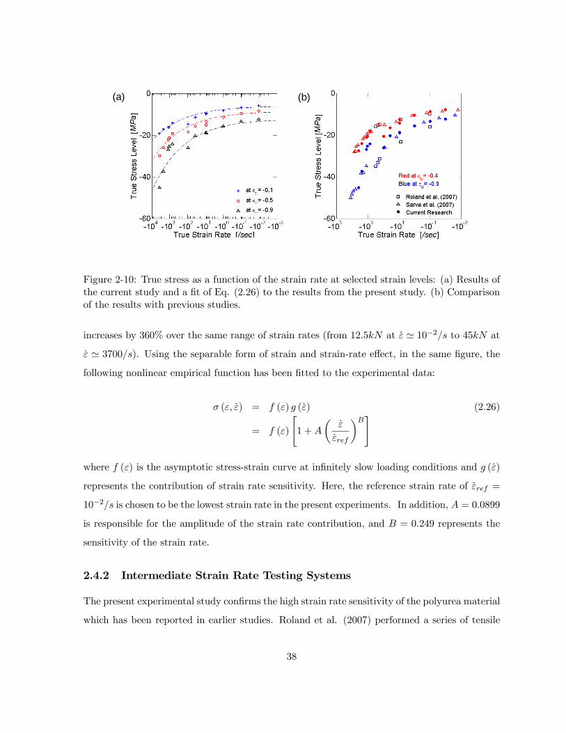
(b)(a)

Figure 2-10: True stress as a function of the strain rate at selected strain levels: (a) Results ofthe current study and a fit of Eq. (2.26) to the results from the present study. (b) Comparisonof the results with previous studies.

increases by 360% over the same range of strain rates (from 12.5kN at ε ' 10−2/s to 45kN at

ε ' 3700/s). Using the separable form of strain and strain-rate effect, in the same figure, the

following nonlinear empirical function has been fitted to the experimental data:

σ (ε, ε) = f (ε) g (ε) (2.26)

= f (ε)

"1 +A

µε

εref

¶B#

where f (ε) is the asymptotic stress-strain curve at infinitely slow loading conditions and g (ε)

represents the contribution of strain rate sensitivity. Here, the reference strain rate of εref =

10−2/s is chosen to be the lowest strain rate in the present experiments. In addition, A = 0.0899

is responsible for the amplitude of the strain rate contribution, and B = 0.249 represents the

sensitivity of the strain rate.

2.4.2 Intermediate Strain Rate Testing Systems

The present experimental study confirms the high strain rate sensitivity of the polyurea material

which has been reported in earlier studies. Roland et al. (2007) performed a series of tensile

38

tests using a custom-made pulley system in a drop tower to perform uniaxial tensile tests at

intermediate and high strain rates. Sarva et al. (2007) used an enhanced universal testing

machine to perform compression experiments at strain rates of up to 80/s while an aluminum

SHPB system with a striker bar length of 3m has been used to perform experiments at strain

rates above 800/s. The comparison of the present experimental data with the results of Sarva

et al. (2007) and Roland et al. (2007) confirms the validity of the measurements with the

modified SHPB system (Figure 2-10b).

The implementation of the deconvolution technique by Bussac et al. (2002) leads to a stable

algorithm that is convenient to use for the reconstruction of dispersive waves in bars based

on redundant measurements. Thus, the theoretical limitation of the duration of experiments

on SHPB systems is successfully overcome. In combination with a hydraulic actuator, the

entire range of low to high strain rates could be covered using a single testing system. The

comparison with conventional SHPB experiments at high strain rates and universal testing

machine experiments at low strain rates has confirmed the validity of the modified SHPB

technique. However, there are still two difficulties associated with our modified SHPB system

which need to be addressed in the future:

• Displacement and/or velocity measurement accuracy: the accuracy of the deconvolution

technique relies heavily on accurate displacement measurements (in particular at low

strain rates). The present optical technique provided good results for loading velocities

of up to 0.5m/s, but significant errors became visible at larger loading velocities.

• Quality of the loading pulse at specimen interfaces. In order to achieve approximately con-

stant strain rates, the ideal loading pulse should be such that the bar/specimen interfaces

move at constant velocities.

The first difficulty may be resolved through the use of improved measurement equipment.

Alternatively, the deconvolution technique for high loading velocities may also be applied using

strain gage measurements only. However, it is very challenging to overcome the second difficulty.

As an intermediate strain rate experiment takes much longer than a wave round trip in the

input bar, the input bar/specimen interface velocity is not constant even if the hydraulic piston

moves at a constant velocity. Simple wave analysis shows that a period of high velocity loading

39

is followed by a period of loading at a lower rate; the length of each period corresponds to the

round trip time for a wave travelling in the input bar. The same holds true for the output

bar/specimen interface velocity which is affected by the round trip time in the output bar.

Consequently, the strain rate in our intermediate strain rate experiments was not constant.

For the desired maximum true compressive strain of ε = 1.0, the total duration of an

intermediate strain experiment at 50/s is Texp = 20ms - irrespective of the specimen geometry.

Conceptually, there exist several solutions to this problem:

• Conventional nylon SHPB system with a striker bar length of 1740× 0.02× 0.5 = 17.4m

along with a 35m long input bar and a 17.5m long output bar. In this configuration, all

strain gages can be positioned such that the rightward and leftward traveling waves do

not superpose at the strain gage locations.

• Conventional nylon SHPB system with a 17.5m long striker bar and 17.5m long input

and output bars. In this case, a deconvolution method needs to be used to reconstruct

the waves in the input and output bars. However, the input bar is still sufficiently long

to guarantee that the round trip time is greater than the duration of the experiment.

• Hydraulic nylon SHPB system with 17.5m long input and output bars. Based on the

assumption that the hydraulic piston moves at a constant velocity, this system will provide

the same capabilities as the previous system.

As an alternative to very long input and output bars, one may chose the opposite strategy.

Note that the magnitude of the oscillations is proportional to the change in force level in

the specimen over the time Tin. Thus, the shorter the input bar, the smaller the oscillation

magnitude. One could therefore envision very short (e.g. < 0.5m) small diameter input and

output bars. In this case, we have Tin = 0.57ms and hence Tin ¿ Texp.

However, since the modified SHPB system requires two displacement measurement sensors

(notably for low strain rate experiments), one can also use these sensors to measure directly

the displacements of the respective bar/specimen interfaces. Hence the strain history can be

measured without using the deconvolution algorithm. The bars would therefore only serve as

load cell to measure the force history. Unless the quasi-static equilibrium needs to be verified

40

experimentally, a single force measurement is satisfactory. Moreover, it may be worth consider-

ing a piezoelectric sensor to measure the force, thereby completely eliminating the use of bars

to perform the experiments at low, intermediate and high strain rates. As our hydraulic piston

cannot provide a constant loading velocity above 0.5m/s, a striker bar may also be used to load

the specimen. The only unknown which is left in this system is the realization of the “fixed”

boundary condition. Further research needs to be carried out to design a support point that

does not introduce spurious oscillation into the testing system.

2.5 Conclusion

The modified SHPB system of Zhao and Gary (1997) has been used to perform compression tests

on polyurea at low, intermediate and high strain rates. It is composed of nylon input and output

bars, while the striker bar is substituted by a hydraulic actuator. Using the deconvolution

technique by Bussac et al. (2002), the time limitation of conventional SHPB systems may be

overcome, thereby enabling the use of the modified SHPB system for low and intermediate strain

rate experiments of long duration. The experiments confirm the known strain rate sensitivity

of polyurea. The measured stress levels correspond well to earlier results which have been

obtained from tests on conventional SHPB systems with very long bars. Although the intrinsic

time limitation of SHPB systems could be overcome, this study also shows that it is still not

possible to perform experiments at reasonably constant strain rates with this technique. This is

due to the finite length of the input and output bars which causes a periodic change in loading

velocity. It is shown that intermediate strain rate SHPB experiments require either very long

bars (> 20m) or very short bars (< 0.5m) in order to achieve an approximately constant strain

rate throughout the entire experiment.

41

Chapter 3

Constitutive Modeling

3.1 Introduction

Polyurea is used to mitigate structural damage during impact loading because of its good

damping performance. In addition, it is utilized by various industries because of its fast setting

time as well as its good chemical and fire resistance. Polyurea has found applications in army

vehicles for blast protection because of its high toughness-to-density ratio at high strain rates.

Polyurea shows a highly nonlinear viscoelastic behavior at finite strains (e.g. Amirkhizi et

al., 2006, Bogoslovov and Roland, 2007, Roland et al., 2007, Shim and Mohr, 2009a). The

mechanical properties of linearly viscoelastic materials may be described by the relaxation

modulus (or creep compliance) which is independent of strain magnitude. However, nonlinear

viscoelasticity is characterized by a decrease (or increase) of the relaxation modulus (or creep

compliance) with increasing strain or decreasing stress (e.g. Brinson and Brinson, 2008).

Most finite viscoelasticity models of elastomers are formulated using either (1) the so-called

hereditary integral approach or (2) the framework of multiplicative decomposition of the de-

formation gradient. Motivated by linear viscoelastic models, hereditary integral models are

formulated in terms of relaxation or memory functions (e.g. Lockett, 1972). Widely used single

integral theories are the theory of Finite Linear Viscoelasticity (Coleman and Noll, 1961) and

the BKZ theory (Bernstein et al., 1963); both make use of several relaxation/memory functions.

Significant efforts have been made to improve these theories and to reduce the number of re-

quired material parameters (e.g. Lianis, 1963, McGuirt and Lianis, 1970, Leonov, 1976, Johnson

42

et al., 1994, Haupt and Lion, 2002). Nonlinear viscoelastic behavior is often considered as the

superposition of a rate-independent nonlinear elastic response (so-called equilibrium part) and a

viscosity-induced overstress contribution which is described through fading memory functions.

Most nonlinear viscoelastic constitutive models have been experimentally validated at very low

strain-rates of 0.1/s or less. Only few papers deal with the nonlinear viscoelastic behavior of

elastomers at intermediate and high strain-rates (1/s to 1000/s). Using the hereditary integral

approach, Yang et al. (2000) and Shim et al. (2004) proposed a phenomenological constitutive

model to predict the behavior of silicon rubber at high strain rates (900/s to 3000/s). Hoo Fatt

and Ouyang (2007) adopted the integral approach to model the response of butadiene rubber at

strain rate ranging from 76/s to 450/s. The validity of most hereditary integral approach based

models is limited to a narrow range of strain rates due to the use of only one relaxation time

period (Yang et al., 2000 and Shim et al., 2004) or a constant memory function (Hoo Fatt and

Ouyang, 2007). In general, the hereditary integral approach is very useful in describing finite

viscoelastic behavior, but its successful application to the real test data depends strongly on

the effectiveness of the rather complex relaxation or memory function calibration procedures.

Compared to hereditary integral models, the multiplicative decomposition of the deforma-

tion gradient typically leads to models with material parameters that can be easily identified

from experiments. The concept of the multiplicative decomposition of the deformation gra-

dient (Kröner, 1960, and Lee, 1969) was initially applied to finite viscoelasticity by Sidoroff

(1974) and further explored by others (e.g. Lubliner, 1985, Le Tallec, 1993, Reese and Govin-

djee, 1998, Huber and Tsakmakis, 2000). The nonlinear viscoelasticity is commonly described

through a rheological spring-dashpot model that features a rate-independent equilibrium part

and a rate-dependent viscous part. In particular, Zener models are widely used (e.g. Roland,

1989, Johnson et al., 1995, Bergström and Boyce, 1998, Huber and Tsakmakis, 2000, Quin-

tavalla and Johnson, 2004, Bergström and Hilbert, 2005, Qi and Boyce, 2005, Tomita et al.,

2008, Areias and Matous, 2008). Zener models are composed of a spring (rate-independent

part) in parallel with a Maxwell element (rate-dependent part). The constitutive model of the

time-dependent part includes an evolution equation for the viscous deformation. The simplest

evolution equation is a linear viscous flow rule (e.g. Amin et al., 2002, Johlitz et al., 2007).

However, experiments have shown that the viscosity at finite strains is a function of the driving

43

stress (e.g. Amin et al., 2006), the strain (e.g. Amin et al., 2006, Hoo Fatt and Ouyang, 2008)

and/or the strain-rate (e.g. Khan et al., 2006). Thus, nonlinear viscous flows rules have been

developed using a micro-mechanism inspired approach (e.g. Bergström and Boyce, 1998, Palm

et al., 2006) or a purely phenomenological approach (e.g. Khan and Zhang, 2001, Colak, 2005,

Amin et al., 2006, Khan et al., 2006, Hoo Fatt and Ouyang, 2008).

In order to represent the equilibrium contribution as the nonlinear elastic spring, rubber

elasticity models are employed using the conventional material types such as Neo-Hookean (e.g.

Johlitz et al., 2007), Mooney-Rivlin, (e.g. Huber and Tsakmakis, 2000), or Arruda and Boyce’s

(1993) eight-chain model (e.g. Bergström and Boyce, 1998, Tomita et al., 2008). Other research

groups (e.g. Amin et al., 2002, 2006, Hoo Fatt and Ouyang, 2008) used modified conventional

material models to describe the high initial stiffness and the subsequent strain hardening.

Although many researcher have recently reported on experimental behavior of various poly-

meric materials for a wide range of strain rates (e.g. Khan and Farrokh, 2006, Mulliken and

Boyce, 2006, Sarva et al., 2007), little research has been reported on the modeling of elastomeric

materials for loading and unloading for a wide range of strain rates. As for the hereditary inte-

gral approach based models, most multiplicative decomposition based models have been exper-

imentally validated for a narrow range of strain rates. Quintavalla and Johnson (2004) adopted

the Bergström-Boyce model to describe the dynamic behavior of cis-(1,4) polybutadiene at high

strain-rate of 3000/s to 5000/s. Recently, Hoo Fatt and Ouyang (2008) proposed a thermo-

dynamically consistent constitutive model with modified neo-Hookean rubber elastic springs

to describe the steep initial stiffness of virgin butadiene rubber under tensile and compressive

loading at intermediate strain rates (76/s to 450/s).

The present work focuses on the modeling of the loading and unloading response of polyurea

over a wide range of strain rates (from 10−3/s to 101/s) and at large compressive strains (up

to 1.0). Using the framework of the multiplicative decomposition of the deformation gradient,

the rheological concept of two parallel Maxwell elements is employed to develop a nonlinear

viscoelastic finite strain constitutive model. Guided by similar developments in area of rate-

dependent plasticity models for glassy polymers (e.g. Qi and Boyce, 2005, Anand and Ames,

2006, Anand et al., 2009, Ames et al., 2009, Ayoub et al., 2009), the high stiffness of elastomers

at small deformations is modeled using Hencky’s strain energy function. In view of the simula-

44

tion of blast and impact events, we limit our attention to the mechanical behavior of polyurea

in its virgin state. After presenting all experimental results in Section 3.2, the constitutive

model is detailed in Sections 3.3 and 3.4. A discussion of the comparison of simulations and

experimental results for polyurea is given in Section 3.5.

3.2 Experimental Investigation

3.2.1 Material

The polyurea specimens used in the study are extracted from a 12.7mm thick polyurea DragonShield-

HT Explosive Resistant Coating (ERC) layer on a steel armor plate. After separation from the

plates, the polyurea specimens of diameter D0 = 10mm and length L0 = 10mm are machined

using conventional milling procedures. The shelf life of the polyurea prior to testing was about

4 years. All experiments are performed on polyurea in its virgin state (condition after curing.

no prior mechanical loading history).

3.2.2 Relaxation Experiments

The nonlinearity of the viscoelastic behavior of polyurea at low and intermediate strain rates

is identified from relaxation tests. Using a hydraulic universal testing machine (Model 8800,

Instron), the material is rapidly loaded to a prescribed strain level at the beginning of the

experiment. The strain is subsequently kept constant while stress relaxation takes place. Nine

relaxation tests are performed for true compressive strains ranging from ε0 = 0.048 to 1.0. The

engineering strain rate during the rapid loading phase was about 0.48/s. In order to capture

the short-term viscoelastic behavior, the sampling frequency of the data was 5kHz; the stress

is recorded for about 10 minutes to identify the long-term behavior. Figure 3-1a shows the

recorded stress histories for various constant strain loadings. While the test duration was not

long enough to observe the asymptotic long-term behavior (i.e. equilibrium modulus), the

results indicate that the sampling frequency of 5kHz is high enough to capture the asymptotic

short-term viscoelastic behavior (i.e. initial relaxation modulus).

45

(e) (f)

(c) (d)

(a) (b)

Figure 3-1: Results of relaxation tests (left column) and corresponding simulations (right col-umn). (a)-(b) True stress histories, (c)-(d) Relaxation moduli histories, (e)-(f) Isochronousstress-strain curves for different instants after the rapid strain loading.

46

The relaxation moduli are computed using the definition

H (t) =σ (t)

ε0(3.1)

where σ (t) is the time history of the measured true stress for a constant strain of ε0 (Figure

3-1a). The corresponding relaxation modulus histories (Figure 3-1c) clearly demonstrate the

nonlinear viscoelastic nature of the material response: the relaxation modulus decreases from

120MPa (at the strain of −0.048) to 20MPa (at the strain of −1.0) at the beginning of

relaxation; after more than 10 minutes, the corresponding relaxation moduli are 60MPa and

10MPa, respectively. The strong nonlinear nature of the viscoelastic behavior becomes also

apparent when plotting the isochronous stress-strain curves (Figure 3-1e).

3.2.3 Continuous Compression Experiments

In addition to relaxation experiments, constant strain rate loading and unloading tests are

performed at absolute true strain rates between 10−3 and 101/s (Figure 3-2a). The measured

true stress versus logarithmic strain curves for five different strain rates are summarized in

Figure 3-2b. At least two tests are performed at each strain rate to confirm the repeatability

of the experimental results. During the loading phase, the observed stress level exhibits strong

strain rate sensitivity. For example, the observed stress level for 10−3/s is about twice as high

as for 101/s. However, during unloading, all the stress-strain curves seem to converge to the

same curve regardless of the unloading strain rate.

3.2.4 Stair Compression Experiments

In order to investigate the stress relaxation behavior during loading and unloading, experiments

are performed with stair-type strain history profiles. Figure 3-3a shows the applied strain history

as a function of the normalized time t |ε/ε0|. The same maximum strain of ε0 = −1.0 is chosen

for all experiments. Experiments are performed for |ε0| = 10−3/s, 10−2/s, 10−1/s, 100/s and

101/s. All measured stress-strain curves are depicted in Figure 3-3b. The results from the stair

compression tests confirm the previous observation of high strain rate sensitivity during loading

phase along with nearly rate independent behavior during unloading. Also the magnitude of

47

(b) (c)

(a)

Figure 3-2: Results of continuous loading/unloading experiments and corresponding simula-tions. (a) History of applied strain. Note that time in the x-axis is normalized by the totaltesting duration |ε0/ε0| where ε0 = 10−3 , 10−2, 10−1, 100, and 101/s . (b) Stress-strain curvesobtained from experiments and

48

stress relaxation during the loading phase is found to be larger than that during unlading. The

superposition of the results from the monotonic and stair compression experiments (Figure 3-

3d) shows that the specimens recover the virgin state resistance (described by the curves from

the monotonic tests) after each relaxation period in the stair compression experiment. The

resistance recovery appears to be slower for large strains and high strain rates.

3.3 Constitutive Model

3.3.1 Motivation

In the framework of multiplicative decomposition of the deformation gradient, models of the

Zener type (Maxwell element in parallel with a spring) are widely used since these can effec-

tively represent the nonlinear viscoelastic behaviors of many elastomers. For Zener models,

it is common to identify the equilibrium path and the over-stress contribution from the ex-

perimental stress-strain curves. The equilibrium path can be determined in an approximate

manner from two alternative approaches: (1) taking the mid-path of stress-strain curves from

the monotonic loading and unloading test (e.g. Bergström and Boyce, 1996), (2) connecting

the stress relaxation mid-points between loading and unloading phase from the stair-type com-

pression tests (e.g. Qi and Boyce, 2005). Figure 3-4 shows the equilibrium paths that have

been identified from the continuous compression tests at different strain rates. The summary

plot in Figure 3-66a clearly shows that the identified equilibrium paths are not identical, i.e.

the identified equilibrium path depends on the strain rate. For instance, at a strain of −1.0,

an equilibrium stress of −10MPa is found from the experiment at 10−3/s while an equilibrium

stress of −17MPa is obtained from the experiment at 101/s. This important observation is

confirmed by the stair-type compression tests. Recall from Figure 3-33b that the amount of

stress relaxation is different for loading and unloading. Thus, it is concluded that the concept

of equilibrium path breaks down in the case of polyurea. Consequently, rheological models of

the Zener type will not be able to describe the nonlinear viscoelastic behavior of polyurea for

both loading and unloading.

In models of the Zener type, the equilibrium part is represented by a spring element. Qi and

Boyce (2005) explained in their paper on the micro-mechanism inspired constitutive modeling

49

(d) (e)

(b) (c)

(a)

Figure 3-3: Results for stair compression loading/unloading. (a) History of applied strain.Note that time in the x-axis is normalized by the total testing duration |ε0/ε0| where ε0 =1 and ε0 = 10−3 , 10−2, 10−1, 100, and 101/s . (b) Stress-strain curves from experimentsand (c) Corresponding simulations. (d) Comparison of results from continuous and stair-typeloading/unloading experiments and (e) Corresponding simulations.

50

(e)

(c) (d)

(a) (b)

Figure 3-4: Estimation of the behavior of Network A using the equilibrium path concept forpath concept for different strain rates: (a) 10−3/s, (b) 10−2/s, (c) 10−1/s, (d) 100/s and (e)101/s

51

Figure 3-5: Proposed rheological model for polyurea composed of two Maxwell elements inparallel.

of thermoplastic polyurethanes that the spring element associated with the equilibrium path

represents the entropic resistance of the soft domains in polyurethanes, while the rate dependent

behavior of the hard part is represented by the Maxwell element of the Zener model. Due to

the apparent rate dependency of the calculated equilibrium paths, we substitute the spring of

the Zener model by another Maxwell element. The resulting rheological model, two Maxwell

springs in parallel (Figure 3-5), has already been considered in the past by Boyce et al. (2000)

and Dupaix and Boyce (2007) to describe the finite strain behavior of amorphous polymers. In

the context of amorphous polymers near glass transition temperature, two Maxwell elements

have been used to represent the rate-dependent inter- and intra-molecular network resistances

under monotonic loading conditions.

In the following, we outline the constitutive equations for each of the four basic elements

of our rheological model. Throughout our presentation, we refer to the Maxwell element that

is predominantly associated with the deformation resistance of the soft domain of polyurea

as “Network A”, while the Maxwell element associated with the effect of the hard domain is

referred to as “Network B”.

3.3.2 Homogenization

The macroscopic deformation gradient Ftot is decomposed into a rotation free volumetric part

Fvol,

Fvol = J1/31 with J = detFtot (3.2)

52

and an isochoric part F

F = J−1/3Ftot (3.3)

The constitutive model for the stresses induced by isochoric deformation is developed with

the Taylor assumption in mind, i.e. the isochoric deformation gradients within both networks,

FA and FB, equal the macroscopic isochoric deformation gradient

F = FA= FB (3.4)

while the deviatoric part of the macroscopic Cauchy stress T corresponds to the spatial average

of the local stress fields

devT =1

Ω

∙ZAσdΩA +

ZBσdΩB

¸(3.5)

where σ describes the local deviatoric stress fields, Ω is the total volume of the representa-

tive volume element, and ΩA and ΩB are the corresponding volumes of Networks A and B,

respectively. In the context of micromechanism-inspired polymer models, the role of the mi-

crostructure is typically neglected. Instead, the constitutive equations for the individual phases

predict a weighted macroscopic Cauchy stress (in the present case the weighted deviator stresses

TA and TB) such that the macroscopic stress deviator can be written as

devT = TA +TB (3.6)

3.3.3 Constitutive Equations for Volumetric Deformation

The volume change of polyurea under mechanical loading is very small as compared to the

magnitude of isochoric deformation. For simplicity, we assume a linear elastic relationship

between the logarithmic volumetric strain and the hydrostatic part of the macroscopic Cauchy

stress tensortrT3= κ

lnJ

J(3.7)

where κ denotes the bulk modulus.

53

3.3.4 Maxwell Model for Isochoric Deformation

The responses of Network A and Network B are described through Maxwell models. In this

subsection, we provide the general framework for the formulation of the constitutive equations

for Maxwell models. In the Sections 3.3.5 and 3.3.6, we will then specialize our equations for

the individual networks.

Kinematics

Consider a Maxwell elementK subject to a isochoric deformation gradient FK with detFK = 1.

In the context of finite strain, we assume that the total isochoric deformation gradient can be

multiplicatively decomposed into an elastic part FeK and a viscous part Fv

K ,

FK = FeKF

vK (3.8)

Furthermore, we introduce the total, elastic and viscous rate of isochoric deformation tensors

FK = LKFK , FeK = L

eKF

eK and Fv

K = LvKF

vK (3.9)

with the relationship

LK = LeK +F

eKL

vKF

e−1K (3.10)

It is assumed that the viscous spins is zero for the deformation of the Maxwell elements.

Formally, we write

DvK := L

vK = L

vTK (3.11)

The rate of deformation tensor DeK may also be expressed as a function of the time derivative

of the right Cauchy-Green tensor

DeK =

1

2Fe−TK Ce

KFe−1K (3.12)

In addition to the tensor description of the kinematics, we make use of the scalar deformation

measure

ζ =√trC− 3 (3.13)

54

in our model formulation. The strain-like variable ζ is zero in the undeformed configuration

and always positive for deformed configurations.

Thermodynamics and Hyperelasticity

For isothermal conditions, the second law of thermodynamics for each Maxwell element reads

JTK : LK − ψK ≥ 0 (3.14)

with the deviatoric Cauchy stress TK and the free energy ψK (per unit initial volume). We

impose the assumption of Green elasticity through the hyperelastic relationship (e.g. Ogden,

1984)

TK =2

Jdev

½FeK

∂ψK

∂CeK

FeTK

¾(3.15)

where CeK = FeT

K FeK denotes the right Cauchy-Green tensor of isochoric elastic deformation.

Recall that we assume isochoric elastic deformation which implies detFeK = 1 and trDe

K = 0.

Using Eq. (3.10) and Eq. (3.15) in Eq. (3.14) yields the thermodynamic constraint

JTK :¡FeKL

vKF

e−1K

¢=³JFeT

K TKFe−TK

´: Dv

K ≥ 0 (3.16)

In the following, the Mandel stress

MK := Jdev©FeTK TKF

eTK

ª(3.17)

is used as the driving stress of viscous deformation while the viscoplastic constitutive equations

are written such that

MK : DvK ≥ 0 (3.18)

Flow Rule for Viscous Flow

The direction of viscous flow is supposed to be aligned with the direction of the driving Mandel

stress. Formally, we write the flow rule

MK = ηKDvK (3.19)

55

with the deformation and rate dependent viscosity ηK ≥ 0. The rate dependent viscosity is

defined through the nonlinear relationship mk = mk

¡dk¢between the equivalent Mandel stress

mk =

r3

2Mk :Mk (3.20)

and the equivalent viscous strain rate

dk =

r3

2Dv

k : Dvk (3.21)

Using Eq. (3.20) and Eq. (3.21) in Eq. (3.19), we obtain

ηK =2

3

mk

dk(3.22)

3.3.5 Specialization of the Maxwell Model for Network A

Network A represents the rubbery response of the soft domain which is modeled through a

Maxwell element composed of a nonlinear elastic Gent spring and a nonlinear viscous damper

that accounts for the apparent rate dependency of the theoretical equilibrium path.

Gent Elasticity of Network A

For isochoric deformation, Gent’s (1996) free energy function may be written as

ψA = −1

2µAJA ln

µ1− trC

eA − 3JA

¶(3.23)

with the material parameters µA > 0 (initial modulus) and JA > 0 (locking stretch). With this

form of free energy, the Cauchy stress TA in Network A reads:

TA =µAJ

µ1− trC

eA − 3JA

¶−1devBe

A (3.24)

where BeA = F

eAF

eTA denotes the right Cauchy-Green tensor of isochoric elastic deformation.

56

Nonlinear Viscous Response of Network A

Figure 3-6a suggests that the viscoelastic contribution to the stress of Network A increases

monotonically as the deformation increases. Furthermore, the experimental results suggest a

power-law relation between the viscosity ηA and the equivalent rate of viscous deformation.

Thus, the nonlinear viscous evolution law for Network A is written as

mA =3

2ηAdA = PA (exp ζ − 1)

µdAdref

¶nA

(3.25)

with the reference rate of deformation dref = 1/s, the viscosity constant PA > 0, and the

exponent nA > 0 controlling the rate-sensitivity.

3.3.6 Specialization of the Constitutive Equations for Network B

Network B represents the response of the hard domain which is modeled through a Maxwell

element composed of a linear elastic spring and a nonlinear viscous damper that accounts for

the high stiffness at small strain and the rate sensitivity of hysteresis.

Hencky Elasticity of Network B

The stiffness of Network B governs the stiff macroscopic response of polyurea at small strains.

Here, we make use of the isochoric part of Hencky’s strain energy function

ψB =1

2µB (lnU

eB) : (lnU

eB) (3.26)

where the elastic stretch tensor UeB is found from the polar decomposition of the elastic defor-

mation gradient, FeB = R

eBU

eB with R

eTB R

eB = 1. Upon evaluation, we obtain the deviatoric

part of the Cauchy stress acting on Network B

TB =2µBJRe

B (lnUeB)R

eTB (3.27)

57

Nonlinear Viscous Response of Network B

Figure 3-7a suggests that the overall viscoelastic response of Network B is similar to the linear

viscoelastic response of a Maxwell model composed of a linear spring (of Young’s modulus E)

and a linear viscous damper (of viscosity η). The stress-strain (σ − ε) response of a Maxwell

model with the linear components at a constant strain rate reads (e.g. Brinson and Brinson,

2008)

σ = Eτε0

∙1− exp

µ− ε

τ ε0

¶¸(3.28)

where τ = η/E is the relaxation time, and ε0 is the applied constant strain rate. Note that

even though the Maxwell model is composed of only linear elements, the stress-strain response

is nonlinear at constant strain rates. However, our experiments suggest that the stress-strain

response of Network B is linear for small strains regardless of strain rate.

Inspired by the results for the one-dimensional Maxwell model with linear components

(Eq. (3.28)), we propose a constitutive equation that guarantees a linear elastic response of

Network B at small strains

mB =√3µBQB

µdBdref

¶nB(1− exp

"− ζ

QB

µdBdref

¶−nB#)(3.29)

where the dimensionless material constants QB and nB characterize the viscous properties of

Network B.

3.4 Identification of the Model Parameters

The proposed constitutive model comprises eight material parameters: four parameters (µA, JA,

PA, nA) for Network A, three parameters (µB, QB, nB) for Network B, and one parameter (κ)

describing the elastic volumetric response. The constitutive equations are detailed for uniaxial

stress loading in order to identify all material parameters from the monotonic loading and

unloading compression experiments.

58

3.4.1 Constitutive Equations for Uniaxial Loading

Under uniaxial stress loading, the macroscopic stress tensor takes the form

T = σe1 ⊗ e1 (3.30)

where σ is the true stress (macroscopic Cauchy stress) while the macroscopic deformation

gradient reads

Ftot = λ1e1 ⊗ e1 + λ2 (e2 ⊗ e2 + e3 ⊗ e3) (3.31)

J = detFtot = λ1 (λ2)2 (3.32)

At the network level, the isochoric part of the deformation gradient may be expressed as a

function of the stretch λ,

F = λe1 ⊗ e1 +1√λ(e2 ⊗ e2 + e3 ⊗ e3) with λ =

µλ1λ2

¶2/3(3.33)

The total stretch of a Maxwell element K can be decomposed further into its elastic part λeK

and the viscous part λvK

λ = λeKλvK (3.34)

Using this notation, the kinematic variables used in our constitutive equations may be

expressed as a function of the elastic and viscous stretches and their respective time derivatives

trCeK = (λ

eK)

2 +2

λeK(3.35)

devBeK =

1

3

∙(λeK)

2 − 1

λeK

¸(2e1 ⊗ e1 − e2 ⊗ e2 − e3 ⊗ e3) (3.36)

lnUeK =

1

2(lnλeK) (2e1 ⊗ e1 − e2 ⊗ e2 − e3 ⊗ e3) (3.37)

ζ =

rλ2 +

2

λ− 3 (3.38)

dk =

¯λvK

¯λvK

(3.39)

59

The deviatoric stress tensors TK acting on the Maxwell elements are written as

TK =σK3(2e1 ⊗ e1 − e2 ⊗ e2 − e3 ⊗ e3) (3.40)

while

σ = σA + σB (3.41)

σA and σB are true stresses acting on Networks A and B, respectively.

Using expressions Eq. (3.30) to Eq. (3.41), we obtain the simplified constitutive equations

for uniaxial loading:

• Volumetric deformation induced linear elasticity with the model parameter κ

σ = 3κlnJ

J(3.42)

• Gent elasticity of Network A with the model parameters JA and µA

σA =µAJ

∙(λeA)

2 − 1

λeA

¸¿1− 1

JA

∙(λeA)

2 +2

λeA− 1¸À−1

(3.43)

• Nonlinear viscous response of Network A with the model parameters PA and nA

|σA| =PAJ(exp ζ − 1)

µdAdref

¶nA

(3.44)

• Hencky elasticity of Network B with the model parameter µB

σB =3µBJlnλeB (3.45)

• Nonlinear viscous response of Network B with the model parameters and ,

|σB| =√3µBQB

J

µdBdref

¶nB(1− exp

"− ζ

QB

µdBdref

¶−nB#)(3.46)

60

Table 3.1: Summary of material parameters indentified from monotonic loading/unloading testsunder five different strain rates.

RubberµA 7.00MPa

Isochoric PartSpring

JA 10.7

of Network AViscous

PA 4.42MPa

DampernA 0.0646

LinearSpring

µB 82.3MPa

Isochoric Partof Network B Viscous

QA 0.0447

DampernA 0.0755

Volumetric Part κ 829MPa

3.4.2 Model Calibration

The 1-D calibration process is composed of two steps: the seven parameters (i.e. µA, JA,

PA, nA, µB, QB and nB) relating to isochoric deformation are identified assuming material

incompressibility (J = 1), before the bulk modulus κ is estimated based on the Lamé moduli

and the Poison’s ratio. A summary of all identified material parameters is given in Table 1.

Material Parameters of Network A (µA, JA, PA, nA)

The model is calibrated such that the response of Network A describes the rate dependency

of the hypothetical equilibrium path in the continuous compression experiments. As discussed

in Section 3.3.1 (see also Figure 3-6a), the hypothetical equilibrium path σA = σA¡λ, dA

¢for

a given strain rate amplitude dA is approximated by the average of the measured loading and

unloading stress-strain curves at a total strain rate ε

σA¡λ, dA

¢' 1

2

£σA¡λ, dA

¢+ σA

¡λ,−dA

¢¤with dA ' |ε| (3.47)

The material parameters for Network A are calibrated in an iterative manner:

61

1. Assuming λeA (t) ' λ (t), we estimate (µA, JA) from the best fit of Eq. (3.4344) to the

experimentally obtained stress-strain curve for the highest strain rate case (here, |ε| '

101/s).

2. For the remaining strain rates, we calculate λeA (t) based on Eq. (3.43) using (µA, JA).

3. Using the relationship λvA (t) = λ (t) /λeA (t), we calculate |σA| as a function of the strain-

like variable ζ for each experiment (Figure 3-6b); in the figure, the curve labels indicate

the average effective viscous strain rate dA.

4. The parameters PA and nA are then obtained from the approximation Eq. (3.44) of the

curves shown in Figure 3-6c.

5. It is useful to evaluate the term ΠA := |σA| / (exp ζ − 1) from each experimental curve.

ΠA is a function of the effective viscous strain rate dA only and independent of the total

strain. In other words, each curve shown in Figure 3-6b reduces to a single data point

in Figure 3-6c. The subsequent curve fit ΠA = (PA/J)¡dA/dref

¢nA of the data points inFigure 3-6c yields the model parameters PA and nA.

After completing Steps 1 to 5, we obtain:

µA = 6.85MPa , JA = 11.0

PA = 4.44MPa , nA = 0.0648(3.48)

A second calibration loop is performed, starting with λeA (t) = λ (t) /λvA (t) in Step 1, where

λvA (t) is the viscous deformation predicted by the model parameters Eq. (3.48). Subsequent

evaluation yields:

µA = 7.00MPa , JA = 10.7

PA = 4.42MPa , nA = 0.0646(3.49)

The calibration procedure has been stopped at this point as additional iterations did not improve

the accuracy of the curve fit.

62

(b) (c)

(a)

Figure 3-6: Material model parameter identification for Network A. (a) Estimated experimen-tal stress-strain curve for Network A; (b) Equivalent Mandel stress as a function of the scalardeformation measure ζ; (c) ΠA as function of the equivalent viscous deformation rate dA forthe identification of the model parameters PA and nA through power-law fit.

63

Material Parameters of Network B (µB, QB, nB)

The stress contribution of Network B is obtained by subtracting the identified stress con-

tribution of Network A (using the parameters Eq. (3.49) in Eq. (3.44)) from the original

stress-strain curve for each strain rate

σB (λ, ε) = σ (λ, ε)− σA¡λ, dA

¢(3.50)

where dA corresponds to the average viscous strain rates that have been determined throughout

the calibration of Network A. Figure 3-7 shows the corresponding results for different strain

rates. According the proposed rheological model, viscoelastic behavior of Network B should

be symmetric with respect to the stress, i.e. σB (λ,−ε) = −σB (λ, ε). However, the curves

in Figure 3-7 illustrate that this symmetry assumption holds only approximately true when

using the calibrated analytical expression Eq. (3.44) for Network A. In close analogy with

the calibration procedure for Network A, we identify the model parameters associated with

Network B:

1. We assume λeB (t) ' λ (t) for the highest strain rate case (i.e. strain rate of 101/s).

2. Determine µB from the best curve fit for the experimental stress-strain curve for the

loading phase using Eq. (3.45).

3. Using µB, we can then calculate λeB (t) and λ

vB (t) = λ (t) /λeB (t) for the other experiments.

The corresponding |σB| versus ζ curves are shown in Figure 3-7b. According to Eq. (3.46),

we have

|σB| =√3µBJ

ζB

∙1− exp

µ− ζ

ζB

¶¸(3.51)

where ζB := QB

¡dB/dref

¢nB is a function of the strain rate only. Thus, we determineζB from the approximation of Eq. (3.51) to the |σB| vs. ζ curves.

4. Subsequently, the material constants QB and nB are found from plotting ζB as a function

of the effective viscous strain rate dB.

64

A second parameter identification loop is performed using λeB (t) = λ (t) /λvB (t) leading to:

µB = 82.3MPa

QB = 0.0447 , nA = 0.0755(3.52)

Bulk Modulus of Material (κ)

The initial shear modulus for the proposed model is the sum of the shear modulus of each

network, i.e., µ = µA + µB = 89.3MPa. Experiments revealed that the Poisson’s ratio of

ν = 0.45 is nearly rate-independent throughout the deformation up to the strain of 1.0 (Shim

and Mohr, 2009a). Since the free energy for the volumetric deformation is based on the linear

elastic model, we can determine the bulk modulus using the relation between the elastic moduli

κ =2µ (1 + ν)

3 (1− 2ν) = 8.29MPa (3.53)

3.5 Comparison of Simulation and Experiments

The constitutive model has been programmed as a user material subroutine for the finite element

software ABAQUS/Explicit. Using the identified material model parameters, we perform the

simulations of all experiments described in Section 3.2.

3.5.1 Continuous Compression

Figure 3-2c summarizes the numerically predicted stress-strain curves for different strain rates.

Similarly to the experiments (Figure 3-2b), the simulation results exhibit a high strain rate

sensitivity during the loading phases. In addition, the characteristic convergence of the stress-

stain curves for different loading velocities is also captured by the simulations. The comparisons

of experiment and simulation for individual strain rates are shown in Figures 3-8a to 3-8e. The

stress-strain curves show a better agreement during loading than during unloading. The loading

portions typically feature the largest error for small strains (less than 0.2) while good predictions

are achieved for large strains. The predicted response during unloading is too stiff for all strain

rates, i.e. the simulations reach a stress of zero at larger compressive strains than measured in

65

(b) (c)

(a)

Figure 3-7: Material model parameter identification for Network B. (a) Estimated experi-mental stress-strain curve for Network B; (b) Equivalent Mandel stress as a function of thescalar deformation measure ζ; (c) ζB as function of the equivalent viscous deformation rate dB;identification of the model parameters QB and nB.

66

the experiments. From an energetic point of view, it is worth noting that the differences during

the loading phase underestimate the mechanical work, while the work is overestimated during

unloading. However, these two errors compensate each other when calculating the viscous

energy dissipation for the entire loading/unloading cycle. In other words, despite small errors

in the stress level during loading and unloading, the overall energy dissipation is well predicted

over a wide range of strain rates.

The graphs in Figure 3-8 also depict the predicted individual contributions of Network A

(dotted blue line) and Network B (dashed green line). During the model calibration, we

assumed that the effective viscous strain rate dA is the same during loading and unloading,

which implies that Network A exhibits the same stress-strain response during loading and

unloading. However, since the total viscous strain λvA keeps on decreasing during unloading (the

driving stress for Network A is compression during both loading and unloading) even though

λ increases, the decrease of the stress level is faster during unloading than the corresponding

increase during loading (hysteresis behavior of a Maxwell element). The differences between

the loading and unloading portion for Network A (blue dashed curves) illustrate this behavior.

The model’s symmetric response of Network B (the green dashed curves show only the

loading portion) is characterized by a plateau over a wide range of strains. Since the elastic

strains in Network B are small, the driving stress of viscous deformation in Network B changes

rapidly from compression during loading to tension during unloading. As a result, the effective

rate of viscous deformation dB is the same during loading and unloading which is consistent with

the assumptions made during calibration. Thus, it is concluded that the differences between

the experiments and model predictions are associated with the response of Network A.

3.5.2 Stair Compression

Figure 3-3c provides an overview on the simulation results for all loading cases next to the

experimentally-measured stress-strain curves from stair compression tests. A direct comparison

of the experimental and the simulation results for each loading velocity is shown in Figure 3-

9a to 3-9e. Overall, we observe the same model accuracy as for the monotonic loading and

unloading experiments, i.e. the model slightly underestimates the stress level for small strains

and predicts a faster decrease in stress level after reversal of the loading direction.

67

(e)

(c) (d)

(a) (b)

Figure 3-8: Comparison of simulation results and experiments for continuous loading-unloadingcycles. (a) 10−3/s, (b) 10−2/s, (c) 10−1/s, (d) 100/s and (e) 101/s

68

(e)

(c) (d)

(a) (b)

Figure 3-9: Comparison of simulation results and experiments for stain loading/unloading. (a)10−3/s, (b) 10−2/s, (c) 10−1/s, (d) 100/s and (e) 101/s

69

The relaxation behavior ofNetwork B is symmetric for loading and unloading (green dashed

lines in Figure 3-9). Conversely, the stress-strain curves for Network A (blue dotted lines in

Figure 3-9) reveal that stress relaxation is more pronounced during the loading phase, while

unloading is mainly elastic. This non-symmetric feature of Network A is also visible at the

macroscopic level where the model predicts the experimental observation of a faster relaxation

during loading than during unloading. The model provides accurate estimates of the relaxation-

induced stress decrease (jump) for small strains during the loading phase, while this decrease

is underestimated at large strains. This is attributed to the fact that the stress contribution

of Network B reaches its plateau level at small strains; as a result, the amplitude of stress

relaxation within Network B is very similar for small and large strains.

3.5.3 Relaxation

Figure 3-1b shows the predicted stress histories for all relaxation experiments. In addition,

the histories of the relaxation modulus are presented in Figure 3-1d. The relaxation modulus

histories are well predicted for the entire range of strains. However, the comparison of the

true stress versus time curves indicates that the model predicts slower stress relaxation than

observed in the experiments. Similar conclusions may be drawn from the comparison of the

experimental and simulated isochronous stress-strain curves. Observe that the instantaneous

stress-strain curves agree well with the test results, while the long-term behavior (e.g. blue

curves for 616s) predicted by the model overestimates the stress level at large strains.

3.5.4 Discussion

The model is able to predict the strain rate dependent loading and relaxation behavior polyurea

with reasonable accuracy. Furthermore, the model provides good estimates of the rate depen-

dent viscous dissipation throughout the loading/unloading cycles. In the present rheological

framework of two parallel Maxwell elements, the identification of the behavior of Network A

is important. Here, the response of Network A has been defined through the “rate-dependent

equilibrium path” concept; the mechanical response of Network A is identical throughout com-

pressive loading and compressive unloading. Furthermore, in the particular case of polyurea,

this imaginary equilibrium path depends on the absolute value of the total true strain rate. The

70

response of the calibrated constitutive model illustrates that the assumption of a Maxwell model

does not lead to an exact description of the material behavior for both loading and unloading.

The hysteresis behavior for loading and unloading at a constant total strain rate is an inherent

feature of Maxwell models. Consequently, the rate dependency of the conceptual equilibrium

path (which is hysteresis free) cannot be represented accurately by a Maxwell model. An at-

tempt has been made to calibrate the material model parameters using a numerical parameter

identification scheme (minimization of the error between the experiments and simulations). In

other words, the equilibrium path concept based separation of the contributions of Network A

and Network B has been omitted throughout the material model parameters identification.

However, the identified model response was not more satisfactory as improvements on the un-

loading response could only be obtained at the expense of the quality of the loading curve

prediction.

In order to come up with an improved constitutive model, one may consider a different rheo-

logical model for Network A, but to the best of the authors’ knowledge, no thermodynamically

consistent model has been published in the open literature that can model the apparent elastic

(same loading and unloading curve), but yet strain rate dependent behavior of Network A.

Thus, alternative modeling approaches need to be explored in the future. One thermody-

namically consistent option is the introduction of loading and unloading conditions for viscous

evolution. However, more research is needed at the microstructural (i.e. molecular) level to

justify such loading and unloading conditions from a mechanism point of view.

3.6 Conclusions

The large strain compression response of polyurea is investigated for strain rates ranging 10−3/s

from to 101/s. Continuous and stair-like loading and unloading experiments are performed in

addition to simple relaxation tests. The experimental results reveal that the so-called equilib-

rium path concept breaks down in the case of polyurea. In contradiction with the definition of

the equilibrium path, the identified average stress-strain curves in continuous loading/unloading

experiments depend on the rate of loading. Thus, as an alternative to the equilibrium path

based rheological models of the Zener type, a new constitutive model is formulated assuming

71

two parallel Maxwell elements. The finite strain constitutive equations are outlined in detail.

Subsequently, the eight material model constants are calibrated to describe the mechanical be-

havior of polyurea. The model predictions are in good agreement with the experimental results.

The characteristic convergence of the unloading paths for different strain rates is successfully

captured by the model. Furthermore, the rate dependent viscous dissipation throughout a load-

ing/unloading cycle is described with reasonable accuracy. The predicted unloading behavior

is too stiff which is associated with the limitations of the Maxwell model that describes the soft

domain of polyurea.

72

Chapter 4

Validation Application

4.1 Introduction

Polyurea is a highly viscoelastic rubber material that is used for the impact protection of vehicle

structures. It is considered for the armor protection and retrofitting of military vehicles that are

exposed to the blast loading of improvised explosive devices. The anticipated effect of polyurea

coatings on the blast resistance of steel plates is twofold. Firstly, the polyurea can directly

absorb a portion of the blast energy as it undergoes large deformations. Secondly, the onset of

ductile fracture of a steel plate may be retarded through the use of a polyurea coating, thereby

increasing the energy absorption of the steel structure.

As discussed by Xue and Hutchinson (2008), necking occurs under uniaxial tension when

the average true stress becomes equal to the overall tangent hardening modulus (Considere

criterion). In the case of a coated ductile substrate, a high strain hardening coating material

can increase the effective hardening modulus of the bilayer material such that necking is re-

tarded with respect to the Considere strain of the uncoated material. The bifurcation analysis

of Guduru et al. (2006) reveals that an added surface layer can increase the resistance of a

structural element to fragmentation. Moreover, their results show that the addition of a soft

coating with high strain hardening can improve the weight specific energy absorption of the

structural element. Xue and Hutchinson (2008) demonstrate that the ratio of the elastomer

modulus to the flow strength of the substrate controls the effect of necking retardation. Mc-

Shane et al. (2008) performed tension and bulge tests on copper/polyurethane bilayers under

73

static and dynamic conditions. Their experimental measurements indicate that coatings do not

provide dynamic performance benefits on an equal mass basis. While the total blast resistance

increases, the weight specific energy absorption of the structure may actually decrease through

the application of a polymer coating. Dynamic ring expansion experiments have been performed

by Zhang et al. (2009) on polyurea coated aluminum 6061 − O and copper 101 at very high

strain rates (4000−15000/s). Their experimental results show that there is no significant effect

of the polyurea coating on the strain at the onset of localization.

It appears that the neck retardation effect in coated ductile substrates is difficult to achieve

when using polyurea in combination with typical engineering materials. However, as pointed

out by McShane et al. (2008), polyurea coatings may still be seen as a practical solution for

enhancing the blast resistance of metallic structures because of the ease of applying polyurea

on existing structures (retrofitting). Even though the performance of the steel substrate may

remain unaffected, a very thick polyurea layer can still increase the energy absorption in absolute

terms. The impulsive loading experiments of Amini et al. (2009a) reveal that polyurea coatings

have a strong effect on the energy transfer to the steel plate. In particular, they demonstrate

that the positioning of polyurea on the impact side promotes failure of the steel plate under

shock loading while a polyurea layer on the back of the plate attenuates the shock. In the present

paper, we deal with the prediction of the large deformation behavior of polyurea in structural

applications. Xue and Hutchinson (2008) made use of a Mooney-Rivlin model for the polymer

coating in their numerical analysis of the polymer/metal bilayers. Zhang et al. (2009) modeled

the behavior of polyurea using a nonlinear hyperelastic material model. However, both uniaxial

compression and tension tests have demonstrated that the mechanical response of polyurea is

highly strain-rate dependent (e.g. Amirkhizi et al., 2006, Roland et al., 2007, Sarva et al., 2007,

Shim and Mohr, 2009a). Amini et al. (2009b) make use of the temperature-, rate- and pressure-

sensitive constitutive model by Amirkhizi et al. (2006) to provide supporting simulation results

of their direct pressure pulse experiments.

Finite viscoelasticity models of elastomers may be formulated using the so-called hereditary

integral approach (Coleman and Noll, 1961, Bernstein et al., 1963, Lianis, 1963, McGuirt and

Lianis, 1970, Leonov, 1976, Johnson et al., 1994, Haupt and Lion, 2002, Amirkhizi et al., 2006)

but their validity is often limited to a narrow range of strain rates (Yang et al., 2000, Shim et al.,

74

2004, Hoo Fatt and Ouyang, 2007). As an alternative to the hereditary integral approach, the

framework of multiplicative decomposition of the deformation gradient (Kröner, 1960 and Lee,

1969) is frequently used in finite viscoelasticity (e.g. Sidoroff, 1974, Lubliner, 1985, Le Tallec

et al., 1993, Reese and Govindjee, 1998, Huber and Tsakmakis, 2000). In that framework,

the nonlinear viscoelasticity of elastomers is commonly described through a rheological spring-

dashpot models of the Zener type (e.g. Roland, 1989, Johnson et al., 1995, Bergström and

Boyce, 1998, Huber and Tsakmakis, 2000, Quintavalla and Johnson, 2004, Bergström and

Hilbert, 2005, Qi and Boyce, 2005, Areias and Matous, 2008, Hoo Fatt and Ouyang, 2008,

Tomita et al., 2008).

In the present work, we present the time integration scheme for a newly developed rate-

dependent constitutive model for polyurea (Shim and Mohr, 2009b). After implementing the

model as a user material subroutine into a commercial finite element software, the model is used

to predict the mechanical response of thick polyurea layers under punch loading. Experiments

are performed on 10mm thick polyurea layers for different punch velocities and different hemi-

spherical punch radii. It is found that the model provides an accurate description of the loading

phase, which validates the assumptions made with respect to strain-rate and pressure sensitiv-

ity. However, the predicted response deviates from the experimental result during unloading

which is discussed in detail.

4.2 Punch Experiments

4.2.1 Specimens

The polyurea specimens used in the study are extracted from a steel armor plate with a 12.7mm

thick layer of polyurea DragonShield-HT Explosive Resistant Coating (ERC). Rectangular sam-

ples of 46×40mm are cut from the coated armor plate using conventional machining. The coated

polyurea is not separated from the steel as the steel serves as specimen support throughout the

punching experiments. However, to guarantee a uniform layer thickness for all specimens, the

outer surface of the polyurea is machined down to a final polyurea thickness of 10mm. All

experiments are performed on polyurea in its virgin state (no prior loading) after a shelf life of

about four years.

75

4.2.2 Experimental Procedure

The specimens are clamped on the table of a hydraulic testing machine (Model 8080, Instron).

The specimens are loaded through hemispherical indenters that are attached to the moving

actuator of the upper crosshead. Two hemispherical indenters of different size are employed:

D = 12.7mm and D = 44.45mm (see Figures 4-1a and 4-1b). In addition, we consider two dif-

ferent types of lateral boundary conditions: (1) free in all lateral directions, and (2) constrained

in the width direction (Figures 4-1c and 4-1d). For the latter case, the polyurea specimen is

placed between two steel blocks which prevents bulging in the width direction, but does not

prevent possible shrinking of the specimen in width direction. The friction at the interface

between the indenters and the polyurea is reduced by grease and multiple 0.1mm thick Teflon

layers (which are partially torn apart during the test). The experiments are performed under

displacement control at constant deceleration using the control software MAX (Instron, Can-

ton). Starting with an initial velocity v0, the velocity-time profile decreases linearly until the

experiment is stopped at a velocity of −v0 (Figure 4-2). The initial position of the actuator

is chosen such that the loading direction is reversed (point v0 = 0) when the punch depth

reaches 7mm. Experiments are performed for v0 = 1mm/s and v0 = 100mm/s. Throughout

all experiments, the punch force is measured using a 50kN load cell. The punch displacement

is measured using an LVDT that is integrated in the actuator. The overall stiffness of the test-

ing frame of about 100kN/mm has obtained from the comparison of the LVDT readout with

optical displacement measurements (Shim and Mohr, 2009a). All displacements reported in the

following have been corrected by the deformation associated with the finite machine stiffness.

4.2.3 Experimental Results

Figure 4-3a summarizes the results for the experiments with the small hemispherical indenter

(D = 12.7mm). The measured force-displacement curves are monotonically increasing up to

the point of load reversal. During unloading, the force reaches zero at a displacement of about

3.2mm. Beyond that point, the punch moves faster than the surface of the creeping polyurea

specimen. The force level is about 40% higher in a punch test at v0 = 100mm/s than that

at v0 = 1mm/s which is mostly due to the rate dependent material behavior. Note that the

76

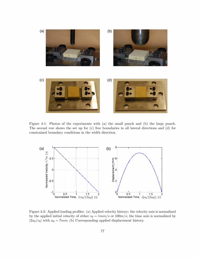
(c) (d)

(a) (b)

Figure 4-1: Photos of the experiments with (a) the small punch and (b) the large punch.The second row shows the set up for (c) free boundaries in all lateral directions and (d) forconstrained boundary conditions in the width direction.

(a) (b)

Figure 4-2: Applied loading profiles: (a) Applied velocity history; the velocity axis is normalizedby the applied initial velocity of either v0 = 1mm/s or 100m/s; the time axis is normalized by|2u0/v0| with u0 = 7mm; (b) Corresponding applied displacement history.

77

(a) (b)

Figure 4-3: Measured load-displacement curves for experiments with (a) the small punch, (b)the large punch.

loading conditions are of quasi-static nature since the speed of elastic waves is polyurea (of

the order of 106mm/s) is much faster than the loading velocities. It is interesting to observe

the convergence of the force-displacement curves for both velocities upon unloading which is

consistent with the results from uniaxial compression experiments (Shim and Mohr, 2009b).

The results with and without constraint in the width direction are almost identical. Thus,

Figure 4-3a presents the results for free lateral boundary conditions only.

In close analogy with the results from the small punch, the measured force-displacement

curves for the large hemispherical punch experiments are loading velocity sensitive and show

a higher force level for the high loading velocity (Figure 4-3b). Moreover, the large punch

experiments also show the characteristic convergence of the force-displacement curves during

unloading. For the large punch, the force level is zero at a punch displacement of 3.4mm. The

effect of the boundary condition in width direction becomes apparent when using the large

hemispherical punch (D = 44.45mm); the force level with the constraint (solid lines) is higher

than that with the free lateral boundary conditions (dotted lines). Regardless of the applied

velocity profiles, the constraint in the width direction increases the force level by about 3kN

at the maximum punching depth. Subtracting the force level with v0 = 1mm/s from the force

level from v0 = 100mm/s for the corresponding displacement magnitude, one can find that the

78

Figure 4-4: Rheological model of the rate dependent constitutive model for polyurea.

effect strain rate during loading phase results in the increase of force level up to 7kN about at

the punching depth of 7mm.

4.3 Constitutive Model

In the following, we present the algorithmic version of a recently-developed constitutive model

for polyurea. The reader is referred to Shim and Mohr (2009b) for details on the differen-

tial formulation and the underlying physical arguments for specific constitutive equations.

The algorithm is implemented as a user material subroutine for the finite element software

Abaqus/explicit. The constitutive equations are based on a rheological model of two Maxwell

elements that act in parallel (Figure 4-4). The first Maxwell element represents the soft part

(Network A) of polyurea and is composed of a nonlinear viscous damper and a nonlinear Gent

spring. The hard part (Network B) is represented by another nonlinear viscous damper and

a Hencky spring. The equations are cast in a framework of finite strains with multiplicative

Kröner-Lee decomposition (Kröner, 1960, and Lee, 1969) of the deformation gradient for each

Maxwell element. The specific evolution laws for individual model components are given in

algorithmic form below. The Euler forward numerical integration method is employed within

the subroutine for the effectiveness of the implementation, because of numerical challenges as-

sociated with Euler backward integration schemes for Maxwell model with nonlinear rubber

spring and nonlinear dashpot (e.g. Areias and Matous, 2008).

The material model comprises the viscous deformation gradients of Networks A and B, FvA

79

and FvB, as internal state variables. We consider the strain driven time integration problem,

where the variables at time τ = t+∆t are calculated based on the solution at time t. In other

words, given the total deformation gradient Ftot (τ) and the internal state variables FvA (t) and

FvB (t), we evaluate the total Cauchy stress T (τ) along with the updated state variables F

vA (τ)

and FvB (τ). The hydrostatic part of the Cauchy stress tensor is directly related to the change

in total volume,

J (τ) = detFtot (τ) (4.1)

trT (τ)3

= κlnJ (τ)

J (τ)(4.2)

where κ denoting the bulk modulus. The deviatoric part of the macroscopic stress tensor corre-

sponds to the sum of the deviatoric stresses TA and TB acting on Network A and Network B,

respectively,

T (τ) = devT (τ) +trT (τ)3

1 (4.3)

= TA (τ) +TB (τ) +trT (τ)3

1

For the evaluation of the stresses and internal variables in Networks A and B, it is useful to

define the isochoric deformation gradient

F (τ) = [J (τ)]−1/3Ftot (τ) (4.4)

as well as the strain-like deformation measure

ζ (τ) =qtr FT (τ)F (τ)− 3 (4.5)

4.3.1 Response of Network A

The viscous gradient is calculated from the Euler forward form

FvA (τ) = [1+∆t D

vA (t)]F

vA (t) (4.6)

80

where DvA (t) is the rate of viscous deformation at time t. Subsequently, we have the isochoric

deformation gradient of elastic deformation in Network A

FeA (τ) = FA (t) [F

vA (t)]

−1 (4.7)

Using FeA (τ), we determine the deviatoric Cauchy stress for Network A based on Gent’s (1996)

free energy function

TA (τ) =µAJ (τ)

Ã1−

tr©FeTA (τ)Fe

A (τ)ª− 3

JA

!−1dev

©FeA (τ)F

eTA (τ)

ª(4.8)

with the material parameters µA > 0 (initial modulus) and JA > 0 (locking stretch).

The viscous rate of deformation tensor DvA (τ) is obtained from the nonlinear viscous evo-

lution law. For this, we calculate the driving Mandel stress

MA (τ) = J (τ)devnFeTA (τ)TA (τ)F

e−TA (τ)

o(4.9)

along with the corresponding equivalent stress

mA (τ) =

r3

2MA (τ) :MA (τ) (4.10)

The equivalent rate of viscous deformation dA (τ) is then given by the power-law

dA (τ) = dref

¿mA (τ)

PA [exp ζ (τ)− 1]

À1/nA(4.11)

with the reference rate of deformation dref = 1/s and the material properties PA > 0 (viscosity

constant) and the exponent nA > 0 (constant for rate sensitivity). The flow rule assumes that

the rate of viscous deformation tensor DvA is aligned with the driving Mandel stress MA

DvA (τ) =

3

2

dA (τ)

mA (τ)MA (τ)

81

4.3.2 Response of Network B

In close analogy with the procedure for Network A, the constitutive equations for Network B

are solved numerically. We have

FvB (τ) = [1+∆t D

vB (t)]F

vB (t) (4.12)

and

FeB (τ) = FB (t) [F

vB (t)]

−1 (4.13)

The stiff elastic response of Network B is described by Hencky’s strain energy function. Thus,

elastic right stretch tensor UeB (τ) and the rotation tensor R

eB (τ) are calculated from the polar

decomposition of the elastic deformation gradient,

FeB (τ) = R

eB (τ)U

eB (τ) with ReT

B (τ)ReB (τ) = 1 (4.14)

before calculating the deviatoric Cauchy stress

TB (τ) =2µBJ (τ)

ReB (τ) [lnU

eB (τ)]R

eTB (τ) (4.15)

with the shear modulus µB.

Subsequently, we write

MB (τ) = J (τ)devnFeTB (τ)TB (τ)F

e−TB (τ)

o(4.16)

mB (τ) =

r3

2MB (τ) :MB (τ) (4.17)

The rate of viscous deformation is approximated by

dB (τ) = dref

*mB (τ)√3µBQB

(1− exp

"−ζ (τ)

QB

µdB (t)

dref

¶−nB#)−1+1/nB(4.18)

where QB and nB are material model parameters that control the rate sensitivity ofNetwork B.

As for Network A, the rate of viscous deformation tensorDvB is aligned with the driving Mandel

82

Table 4.1: Summary of material parameters indentified from monotonic loading/unloading testsunder five different strain rates.

RubberµA 7.00MPa

Isochoric PartSpring

JA 10.7

of Network AViscous

PA 4.42MPa

DampernA 0.0646

LinearSpring

µB 82.3MPa

Isochoric Partof Network B Viscous

QA 0.0447

DampernA 0.0755

Volumetric Part κ 829MPa

stressMB

DvB (τ) =

3

2

dB (τ)

mB (τ)MB (τ) (4.19)

4.3.3 Model Parameter Identification

The constitutive model requires the identification of eight material parameters: four parameters

(µA, JA, PA, nA) for Network A, three parameters ( µB, QA, nA) for Network B, and one

parameter (κ) describing the elastic volumetric response. All model parameters have been iden-

tified based on the results from uniaxial compression experiments at five different strain rates

between 10−3/s and 101/s up to a true strain of −1.0. Details on the parameter identification

procedure are given in Shim and Mohr (2009b). Table 4.1 summarizes the identified material

parameters which are used in the present structural validation study. The comparison of the

measured and predicted stress-strain curves for uniaxial compression is shown in Figure 4-5. It

is noted that the present choice of material model parameters provides a good description of the

initial monotonic loading response of polyurea, while the model predictions are systematically

too stiff during unloading.

83

(e)

(c) (d)

(a) (b)

Figure 4-5: Comparison of simulation results and experiments for continuous loading-unloadingcycles. (a) 10−3/s, (b) 10−2/s, (c) 10−1/s, (d) 100/s, (e) 101/s.

84

4.4 Numerical Simulations of the Punch Experiments

Finite element simulations are performed of all punch experiments. We make use of the sym-

metry of the mechanical system by using a quarter model. The polyurea block is meshed with

eight-node reduced integration solid elements (type C3D8R of the Abaqus element library)

while using the user material option to describe the constitutive behavior. The punches are

modeled using rigid elements. The meshes comprise eight elements in thickness direction and

a small bias in the horizontal plane providing a smaller element size near the center than at

the specimen boundaries. Frictionless interface conditions are assumed between the punch and

the polyurea. The motion of all nodes at the bottom of the polyurea (which corresponds to the

interface with the steel substrate in the experiment) is set to zero. We applied the same punch

velocity histories as in the experiments and omitted addition of bulk viscosity.

The deformed meshes at the point of maximum penetration (u0 = 7mm) are shown in Figure

4-6 for the simulation without lateral constraint along the width direction. The comparison of

Figures 4-6a and 4-6b clearly shows that the bulging effect, i.e. the lateral expansion of the

polyurea block is more pronounced for the large than for the small punch. In the latter case,

we observe a small lateral displacement of about 0.5mm. The bulging has little effect in the

load-displacement curves for the small punch and we found nearly the same force-displacement

curve for free and constrained lateral boundary conditions.

The predicted force-displacement curves for the small punch are shown in Figure 4-7a.

The simulations results are in good agreement with the measured force-displacement curves

during the loading phase. A similar conclusion may be drawn from comparing the simulations

and experiments for the large punch (Figure 4-7b and 4-7c). The comparison shows that the

numerical model can predict (a) the effect of the punch size, (b) the effect of the lateral boundary

constraint, and (c) the effect of loading velocity on the force-displacement curve during loading.

Figure 4-8 shows the histories of the strain-like variable, ζ, and the viscous rates, dA and

dB, for the simulation of a small punch with v0 = 100mm/s (the corresponding locations are

highlighted in Figure 4-6a). The profiles elucidate the strong variations in local strain rate

during the punch experiments. It is interesting to see that the local viscous rate can be as high

as 30/s which is close to the strain rate of the fastest calibration experiment (Figure 4-5e).

However, unlike for the calibration experiments, the strain rates are non-constant throughout

85

(b)

(a)

Figure 4-6: The contour plots of the logarithmic strain in thickness-direction from simulationswith v0 = 100m/s at an indentation depth of 7mm: (a) small hemispherical indenter, and (b)large hemispherical indenter. The detail in Figure 4-6a shows the locations for which the strainrates dA and dB are plotted in Figure 4-8.

86

a punch tests which is seen as an important validation of the model assumptions with respect

to the effect of strain rate. At a punching depth of 7mm, the simulation results overestimate

the force level by about 0.5kN in the case of the small punch and 2.5kN in the case of the

large punch. This overestimation (which corresponds to less than 10% of the current force

level) is consistent with the model calibration results. Recall from Figure 4-5 that the model

systematically overestimates the stress level at very large compressive strains.

The model predictions during unloading deviate from the experimentally-measured force-

displacement responses. The simulations predict the characteristic convergence of the load-

displacement curves, but the predicted response during unloading is too stiff for both velocities

and both punch sizes. Consequently, the instantaneous residual displacement at zero force

is overestimated in the simulations. This deviation is again consistent with the calibration

experiments, indicating an inherent shortcoming of the model formulation for unloading.

4.5 Discussion on Unloading Behavior of Polyurea

The loading response of the model agrees well with the test results except for an overestimation

of the force at large punch displacements. The simulation results indicate that the material is

subject to strains of up to −2.0 as the punching depth reaches 7mm (see Figure 4-6). Since

this is twice as high as in the experiments for the material model parameter identification, we

performed additional material tests at a strain rate of 10−2/s. Figure 4-9a shows the resulting

stress-strain curve from three different experiments. Each virgin-state specimen is subject to a

single loading-unloading cycle up to a maximum strain of -0.5, -1.0 and -1.5, respectively. The

corresponding simulations (Figure 4-9b) reveal that the numerically-predicted locking behavior

is more severe than that observed in the experiments.

The unloading path in the stress-strain curves comprises two characteristic regimes: a stiff

part at the beginning of unloading followed by a soft part as the stress approaches zero. Both

the experiments and the numerical simulations exhibit this feature. The numerical model does

not show the smooth transition between these two regimes, but this is seen as an acceptable

engineering approximation of the physical behavior. However, the apparent main deficiency of

the current model is its inability to capture the increase of the hysteresis loop width as the strain

87

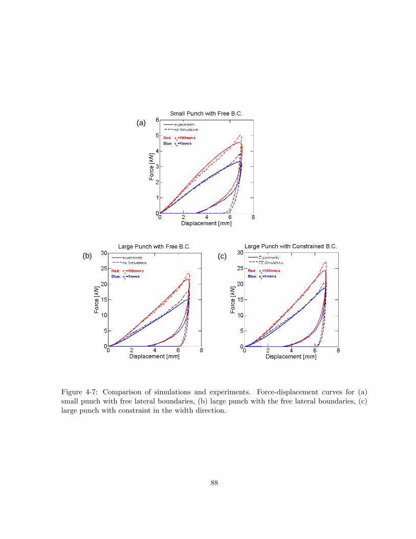
(b) (c)

(a)

Figure 4-7: Comparison of simulations and experiments. Force-displacement curves for (a)small punch with free lateral boundaries, (b) large punch with the free lateral boundaries, (c)large punch with constraint in the width direction.

88

(b) (c)

(a)

Figure 4-8: Results from the small punch simulation with v0 = 100mm/s and free lateralboundary conditions at three different locations (labeled by A, B and C in Figure 4-6(a):Histories of (a) the strain-like deformation measure, ζ, (b) the viscous strain rate of Network A,dA, (c) the viscous strain rate of Network B, dB. Note that the loading direction is reversedat t = 0.14s.

89

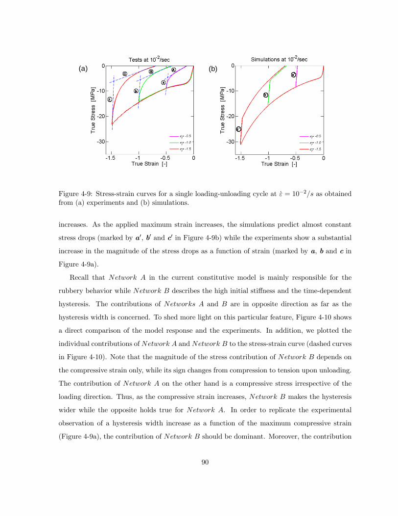
(a) (b)

Figure 4-9: Stress-strain curves for a single loading-unloading cycle at ε = 10−2/s as obtainedfrom (a) experiments and (b) simulations.

increases. As the applied maximum strain increases, the simulations predict almost constant

stress drops (marked by a0, b0 and c0 in Figure 4-9b) while the experiments show a substantial

increase in the magnitude of the stress drops as a function of strain (marked by a, b and c in

Figure 4-9a).

Recall that Network A in the current constitutive model is mainly responsible for the

rubbery behavior while Network B describes the high initial stiffness and the time-dependent

hysteresis. The contributions of Networks A and B are in opposite direction as far as the

hysteresis width is concerned. To shed more light on this particular feature, Figure 4-10 shows

a direct comparison of the model response and the experiments. In addition, we plotted the

individual contributions ofNetwork A and Network B to the stress-strain curve (dashed curves

in Figure 4-10). Note that the magnitude of the stress contribution of Network B depends on

the compressive strain only, while its sign changes from compression to tension upon unloading.

The contribution of Network A on the other hand is a compressive stress irrespective of the

loading direction. Thus, as the compressive strain increases, Network B makes the hysteresis

wider while the opposite holds true for Network A. In order to replicate the experimental

observation of a hysteresis width increase as a function of the maximum compressive strain

(Figure 4-9a), the contribution of Network B should be dominant. Moreover, the contribution

90

of Network B would need to increase as the compressive strain increases. However, due to the

specific choice of the viscous evolution law forNetwork B, the stress contribution of Network B

is more or less constant once the compressive strain has exceeded −0.1 (see the stress plateau

in the response curves for Network B in Figure 4-10). An attempt was made to change

the calibration of the response of Network B using the present modeling framework, but the

subsequent simulation results were no longer satisfactory for the phase of loading.

A constitutive model with a different rheological composition needs to be used to improve

the predictions for unloading. A previous study (Shim and Mohr, 2009b) has shown that

models of the Zener-type (spring in parallel with a single Maxwell element) cannot describe

the large deformation behavior of polyurea over a wide range of strain rates. The present

results indicate that the assumption of two Maxwell elements in parallel provides an accurate

description for monotonic loading only. It can describe the two characteristic stiff and soft

regimes during unloading over a wide range of strain rates, but the model predictions are only

in poor quantitative agreement during unloading.

Throughout our model development, we focused on a single loading-unloading cycle on

virgin-state specimens. However, even though the loading of the material in its virgin state

appears to be the most important with respect to the real-life applications of polyurea, the

material response to cyclic loading may be instructive as far as the choice of the rheological

model is concerned. Figure 4-11 shows the stress-strain curve for polyurea for five consecutive

loading-unloading cycles. After each loading-unloading cycle at a constant true strain rate of

10−2/s, we let the specimen creep at zero stress for about 300s before applying the subsequent

loading-unloading cycle. The significant difference between the first and subsequent loading

cycles illustrates the Mullins effect for polyurea. The stress-strain curve for the first loading is

characterized by the high initial stiffness and the high peak stress marked as A. After the first

loading-unloading cycle, however, the shape of the loading path changes noticeably while nearly

the same unloading path is observed. Additional loading-unloading cycles create very little

changes in both loading and unloading. This observation suggests that the constitutive model

should comprise an internal variable that reflects the amount of “microstructural damage”

associated with the Mullins effect. The Mullins effect has been investigated by many research

groups using either damage-based constitutive models (e.g., Simo, 1987, Govindjee and Simo,

91

(b)

(a)

(c)

Figure 4-10: Comparison of simulation results and experiments for continuous load-ing/unloading cycles at ε = 10−2/s. (a) εf = −0.5, (b) εf = −1.0, (c) εf = −1.5.

92

Figure 4-11: Illustration of the Mullins effect. Five compression loading and unlading cyclesare performed at the constant strain rate of 10−2/s up to the maximum strain of −1.0. Thestress is zero between subsequent cycles for about five minutes.

1991, 1992, Lion, 1996, 1997, Miehe and Keck, 2000) or the concept of hard/soft domain

reorganization (e.g. Johnson and Beatty, 1993a, 1993b, Beatty and Krishnaswamy, 2000, Qi

and Boyce, 2004, 2005). Here, the explicit account of the Mullins effect is deferred to future

work since further experimental data is needed to analyze the effect of loading velocity over a

wide range of strain rates.

4.6 Conclusion

Punch experiments have been performed on 10mm thick polyurea samples at punch velocities

of up to 100mm/s which resulted in maximum local viscous strain rates of up to 30/s inside the

polyurea layers. A newly-developed rate-dependent constitutive model for polyurea has been

implemented into a finite element program and used to predict the experimentally-measured

force-displacement curves for different punch sizes and velocities. Furthermore, the effect of

lateral constraints has been investigated. The model provides accurate predictions of the load-

ing response for all six test configurations which is interpreted as a partial validation of the

assumptions made with respect to strain-rate and pressure sensitivity. During unloading, the

93

model exhibits the characteristic stiff and soft responses of polyurea; however, it systematically

overestimates the depth of the quasi-instantaneous residual punch imprint after unloading.

94

Chapter 5

Conclusion and Suggestions

5.1 Summary of Main Results

The main results of this dissertation can be summarized twofold: experiments and constitutive

modeling. First, the effect of strain rate on polyurea are experimentally quantified for a wide

range of strain rates, i.e. 10−3/s ∼ 4000/s. The modified SHPB system of Zhao and Gary

(1997) has been used to perform compression tests on polyurea at low, intermediate and high

strain rates (10/s ∼ 1000/s). It is composed of nylon input and output bars, while the striker

bar is substituted by a hydraulic actuator. Using the deconvolution technique by Bussac et al.

(2002), the time limitation of conventional SHPB systems may be overcome, thereby enabling

the use of the modified SHPB system for low and intermediate strain rate experiments of

long duration. The experiments confirm the known strain rate sensitivity of polyurea. The

measured stress levels correspond well to earlier results which have been obtained from tests

on conventional SHPB systems with very long bars.

Second, a new constitutive model is proposed to capture the rate-sensitivity for a wide range

of strain rates and the characteristic high stiffness behavior of virgin polyurea at small strains.

Various types of loading conditions are tested for the purpose of validation, and their results

are well compared with the model predictions in loading phases. The large strain compression

response of polyurea is investigated for strain rates ranging 10−3/s from to 101/s. Continuous

and stair-like loading and unloading experiments are performed in addition to simple relaxation

tests. The experimental results reveal that the so-called equilibrium path concept breaks down

95

in the case of polyurea. In contradiction with the definition of the equilibrium path, the iden-

tified average stress-strain curves in continuous loading/unloading experiments depend on the

rate of loading. Thus, as an alternative to the equilibrium path based rheological models of the

Zener type, a new constitutive model is formulated assuming two parallel Maxwell elements.

The finite strain constitutive equations are outlined in detail, and it has been implemented

into a finite element program. Subsequently, the eight material model constants are calibrated

to describe the mechanical behavior of polyurea. The model predictions are in good agree-

ment with the experimental results. The characteristic convergence of the unloading paths for

different strain rates is successfully captured by the model. Furthermore, the rate dependent

viscous dissipation throughout a loading/unloading cycle of uniaxial conditions is described

with reasonable accuracy. For the validation of the proposed model, punch experiments have

been performed on 10mm thick polyurea samples at punch velocities of up to 100mm/s which

resulted in maximum local viscous strain rates of up to 30/s inside the polyurea layers. The

proposed constitutive model is used to predict the experimentally-measured force-displacement

curves for different punch sizes and velocities. Furthermore, the effect of lateral constraints has

been investigated. The model provides accurate predictions of the loading response for all six

test configurations which is interpreted as a partial validation of the assumptions made with

respect to strain-rate and pressure sensitivity.

5.2 Suggestions for Future Studies

The following topics can be suggested for future studies:

• Constant strain rates from the hydraulic SHPB : Although the intrinsic time limitation

of SHPB systems could be overcome, this study also shows that it is still not possible

to perform experiments at reasonably constant strain rates with this technique. This is

due to the finite length (i.e. 3m in this study) of the input and output bars which causes

a periodic change in loading velocity. It is shown that intermediate strain rate SHPB

experiments require either very long bars (> 20m) or very short bars (< 0.5m) in order

to achieve an approximately constant strain rate throughout the entire experiment.

• Improvement in the fixed boundary conditions in the hydraulic SHPB : In order to prevent

96

the failure of the nylon bars under excessive loads, a fixed end support system in the

hydraulic SHPB of the current study is designed such that the bars are released before

elastic buckling occurs. However, with the current design of the fixed end, significant

force drops are found during tests due to the premature partial failure of the fixed end

support of the output bar. A new design of the fixed end support can be investigated to

prevent the elastic buckling of the bars and to resist the specimen strength at the same

time.

• Improvement in the unloading prediction of the constitutive model : From various tests

with different loading conditions, the model exhibits the characteristic stiff and soft re-

sponses of polyurea during unloading. However, the predicted unloading behavior is too

stiff, and the model systematically overestimates the depth of the quasi-instantaneous

residual strain/displacement after unloading. A new rheological model can be investi-

gated to improve the prediction of unloading behavior and to capture the Mullins effect

for polyurea.

97

Appendix A

Identification of the Wave

Propagation Coefficient for

Viscoelastic Bars

The complex-valued propagation coefficient ξ (ω) is a function of both the geometric and ma-

terial properties of the bars. If the complex modulus of the viscoelastic bar material is known,

ξ (ω) may be calculated from solving Pochhammer-Chree’s frequency equation (Zhao and Gary,

1995). As an alternative, we make use of an experimental method that considers both geometric

dispersion and viscous attenuation within the framework of the 1-D wave theory (e.g. Bacon,

1998, Lundberg and Blanc, 1988) to determine ξ (ω). Recall the solution of the one-dimensional

wave equation for viscoelastic bars,

ε (x, ω) = εR (ω) e−iξ(ω)x + εL (ω) e

iξ(ω)x (A.1)

where εR (x, ω) and εL (x, ω) are the rightward and the leftward traveling strain waves. Here,

ξ (ω) is the propagation coefficient of the bars defined by

ξ (ω) = κ (ω) + iα (ω) =ω

c (ω)+ iα (ω) (A.2)

98

where κ (ω) is the wave number, c (ω) is the frequency-dependant longitudinal wave propagation

speed, and α (ω) ≤ 0 represents the attenuation coefficient. Note that c (ω) and α (ω) are even

functions of ω while κ (ω) is an odd function in the frequency space.

After performing an impact test on a single bar, we measure the incident and reflected

strain histories (i.e. εinc (x = 0, t) and εref (x = 0, t)) at x = 0 within in the bar. In order to

determine the transfer function of the bar, we use the two facts from the impact test:

• The rightward and the leftward travelling strain waves are equal to the measured incident

and reflected strain histories, respectively:

εR (ω) = εinc (x = 0, ω) (A.3)

εL (ω) = εref (x = 0, ω) (A.4)

• The normal force is zero at the free end of the bar (i.e. the opposite end to the impacting

end of the bar):

εR (ω) e−iξ(ω)d + εL (ω) e

iξ(ω)d = 0 (A.5)

where x = d is the distance between the strain gage location and the free end of the bar.

Now, the transfer function of the bar H (ω) is experimentally determined from

H (ω) = − εref (x = 0, ω)εinc (x = 0, ω)

= e−2iξ(ω)d (A.6)

From Eq. (A.6), two components of the propagation coefficient can be identified using the

relations

κ (ω) = −arg [H (ω)]2d

(A.7)

α (ω) =ln [|H (ω)|]

2d(A.8)

99

Appendix B

List of Papers with Reference to

Respective Chapters

The following papers are published or submitted for publication with reference to the respective

chapters.

Chapter 2

Shim, J. and Mohr, M. (2009) "Using split Hopkinson pressure bars to perform large strain

compression tests on polyurea at low, intermediate and high strain rates," International Journal

of Impact Engineering, 36:1116-1127.

Chapter 3

Shim, J. and Mohr, M. (2009) "Finite strain constitutive model of polyurea for a wide range

of strain rates," (submitted for publication, September 2009).

Chapter 4

Shim, J. and Mohr, M. (2009) "Punch indentation of polyurea at different loading velocities:

Experiments and numerical simulations," (submitted for publication, October 2009).

100

Bibliography

[1] Aloui, S., Othman, R., Poitou, A., Guégan, P. and El-Borgi, S. (2008) "Non-parametric

identification of the non-homogeneous stress in high strain-rate uni-axial experiments,"

Mechanics Research Communications, 35:392—397.

[2] Ames, N.M., Srivastava, V., Chester, S.A. and Anand, L. (2009) "A thermo-mechanically

coupled theory for large deformations of amorphous polymers. Part II: Applications,"

International Journal of Plasticity, 25:1495-1539.

[3] Amin, A.F.M.S., Alam, M.S. and Okui, Y. (2002) "An improved Hyperelasticity relation

in modeling viscoelasticity response of natural and high damping rubbers in compres-

sion: Experiments, parameter identification and numerical verification," Mechanics of

Materials, 34:75-95.

[4] Amin, A.F.M.S., Lion, A., Sekita, S. and Okui, Y. (2006) "Nonlinear dependence of vis-

cosity in modeling the rate-dependent response of natural and high damping rubbers in

compression and shear: Experimental identification and numerical verification," Interna-

tional Journal of Plasticity, 22:1610-1657.

[5] Amini, M.R., Isaacs, J. and Nemat-Nasser, S. (2009a) "Investigation of effect of polyurea

on response of steel plates to impulsive loads in direct pressure-pulse experiments," Me-

chanics of Materials, in press, doe: 10.1016/j.mechmat.2009.09.008.

[6] Amini, M.R., Simon, J. and Nemat-Nasser, S. (2009b) "Numerical modeling of effect of

polyurea on response of steel plates to impulsive loads in direct pressure-pulse experi-

ments," Mechanics of Materials, in press, doe: 10.1016/j.mechmat.2009.09.009.

101

[7] Amirkhizi, A.V., Isaacs, J., McGee, J. and Nemat-Nasser, S. (2006) "An experimentally-

based viscoelastic constitutive model for polyurea, including pressure and temperature

effects," Philosophical Magazine, 86:5847—5866.

[8] Anand, L. and Ames, N.M. (2006) "On modeling the micro-indentation response of an

amorphous polymer," International Journal of Plasticity, 22:1123-1170.

[9] Anand, L., Ames, N.M., Srivastava, V. and Chester, S.A. (2009) "A thermo-mechanically

coupled theory for large deformations of amorphous polymers. Part I: Formulation," In-

ternational Journal of Plasticity, 25:1474-1494.

[10] Areias, P. and Matous, K. (2008) "Finite element formulation for modeling nonlin-

ear viscoelastic elastomers," Computational Methods in Applied Mechanical Engineering,

197:4702-4717.

[11] Arruda, E.M. and Boyce, M.C. (1993) "A 3-dimensional constitutive model for the large

stretch behavior of rubber elastic materials," Journal of the Mechanics and Physics of

Solids, 41:389-412.

[12] Ayoub, C., Zaïri F., Naït-Abdelaziz, M. and Gloaguen, J.M. (2009) "Modelling large

deformation behaviour under loading-unloading of semicrystalline polymers: Appli-

cation to a high density polyethylene," International Journal of Plasticity, in press,

doi:10.1016/j.ijplas.2009.07.005.

[13] Bacon, C. (1998) "An experimental method for considering dispersion and attenuation in

a viscoelastic Hopkinson bar," Experimental Mechanics, 38:242—249.

[14] Bacon, C. (1999) "Separation of waves propagating in an elastic or viscoelastic Hopkinson

pressure bar with three-dimensional effects," International Journal of Impact Engineering,

22:55—69.

[15] Beatty, M.F. and Krishnaswamy, S. (2000) "A theory of stress-softening in incompressible

isotropic materials," Journal of the Mechanics and Physics of Solids, 48:1931-1965.

102

[16] Bergström, J.S. and Boyce, M.C. (1998). "Constitutive modeling of the large strain

time-dependent behavior of elastomers," Journal of the Mechanics and Physics of Solids,

46:931-954.

[17] Bergström, J.S. and Hilbert, L.B. (2005) "A constitutive model of predicting the large

deformation thermomechanical behavior of fluoropolymers," Mechanics of Materials,

37:899-913.

[18] Bernstein, B., Kersley, E.A. and Zapas, L.J. (1963) "A study of stress relaxation with

finite strain," Transaction of the Society of Rheology, 7:391-410.

[19] Bogoslovov, R.B. and Roland, C.M. (2007) "Viscoelastic effects on the free retraction of

rubber," Journal of Applied Physics, 102:063531.

[20] Bordonaro, C.M. and Krempl, E. (1992) The effect of strain rate on the deformation and

relaxation behavior of 6/6 nylon," Polymer Engineering and Science, 32:1066—1072.

[21] Boyce, M.C., Parks, D.M. and Argon, A.S. (1988) "Large inelastic deformation of glassy

polymers. Part I: Rate dependent constitutive model," Mechanics of Materials, 7:15—33.

[22] Boyce, M.C., Socrate, S. and Llana, P.G. (2000) "Constitutive model for the finite defor-

mation stress-strain behavior of poly(ethylene terephthalate) above the glass transition,"

Polymer, 41:2183-2201.

[23] Brinson, H.F. and Brinson, L.C. (2008) Polymer Engineering Science and Viscoelasticity:

An Introduction, New York, NY, Springer Science+Business Media, LLC, p327.

[24] Bussac, M.N., Collet, P., Gary, G. and Othman, R. (2002) "An optimization method for

separating and rebuilding one-dimensional dispersive waves form multi-point measure-

ments. Application to elastic or viscoelastic bars," Journal of the Mechanics and Physics

of Solids, 50:321—349.

[25] Cady, C.M., Blumenthal, W.R., Gray, G.T. and Idar, D.J. (2003) "Determining the

constitutive response of polymeric materials as a function of temperature and strain rate,"

Journal de Physique IV, 110:27—32.

103

[26] Casem, D.T., Fourney, W. and Chang P. (2003) "Wave separation in viscoelastic pressure

bars using single point measurements of strain and velocity," Polymer Testing, 22:155—

164.

[27] Chen, W., Zhang, B. and Forrestal M.J. (1999) "A split Hopkinson bar technique for low

impedance materials," Experimental Mechanics, 39:81—85.

[28] Chou, S.C., Roberstson, K.D. and Rainey, J.H. (1973) "The effect of strain rate and

heat developed during deformation on the stress—strain curve of plastics," Experimental

Mechanics, 13:422—432.

[29] Colak, O.U. (2005) "Modeling deformation behavior of polymers with viscoplasticity the-

ory based on overstress," International Journal of Plasticity, 21:145-160.

[30] Coleman, B.D. and Noll, W. (1961) "Foundations of linear viscosity," Reviews of Modern

Physics, 33:239-249.

[31] Dupaix, R.B. and Boyce, M.C. (2007) "Constitutive modeling of the finite strain behavior

of amorphous polymers in and above the glass transition,"Mechanics of Materials, 39:39-

52.

[32] Gent, A.N. (1996) "A new constitutive relation for rubber," Rubber Chemistry and Tech-

nology, 69:59-61.

[33] Govindjee, S. and Simo, J. (1991) "A micro-mechanically based continuum damage model

for carbon black-filled rubbers incorporating Mullins effect," Journal of the Mechanics and

Physics of Solids, 39: 87-112.

[34] Govindjee, S. and Simo, J. (1992) "Mullins effect and the strain amplitude dependence

of the storage modulus," International Journal of Solids and Structures, 29:1737-1751.

[35] Graff, K.F. (1975)Wave Motion in Elastic Solids, Mineola, NY, Dover Publications, Inc.,

p470.

[36] Gray, G.T. and Blumenthal, W.R. (2000) "Split-Hopkinson pressure bar testing of soft

materials," ASM Handbook Volume 8: Mechanical Testing and Evaluation, 8:488—496.

104

[37] Gray, G.T., Blumenthal, W.R., Trujillo, C.P. and Carpenter, R.W. (1997) "Influence of

temperature and strain rate on the mechanical behavior of Adiprene L-100," Journal de

Physique IV, 7:523—528.

[38] Grolleau, V., Gary, G. and Mohr, D. (2008) "Biaxial testing of sheet materials at high

strain rates using viscoelastic bars," Experimental Mechanics, 48:293—306.

[39] Guduru, P.R., Bharath, M.S. and Freund, L.B. (2006) "The influence of a surface coating

on the high-rate fragmentation of a ductile material," International Journal of Fracture,

137:89-108.

[40] Haupt, P. and Lion, A. (2002) "On finite linear viscoelasticity of incompressible isotropic

materials," Acta Mechanica, 159:87-124.

[41] Hillström, L., Mossberg, M. and Lundberg, B. (2000) "Identification of complex modulus

from measured strains on an axially impacted bar using least squares," Journal of Sound

and Vibration, 230:689—707.

[42] Hoo Fatt, M.S. and Bekar, I. (2004) "High-speed testing and material modeling of unfilled

styrene butadiene vulcanizates at impact rates," Journal of Materials Science, 39:6885—

6899.

[43] Hoo Fatt, M.S. and Ouyang, X. (2007) "Integral-based constitutive equation for rubber

at high strain rates," International Journal of Solids and Structures, 44:6491-6506.

[44] Hoo Fatt, M.S. and Ouyang, X. (2008) "Three-dimensional constitutive equations for

styrene butadiene rubber at high strain rates," Mechanics of Materials, 40:1-16.

[45] Huber, N. and Tsakmakis, C. (2000) "Finite deformation viscoelasticity laws,"Mechanics

of Materials, 32:1-18.

[46] Jacquelin, E. and Hamelin, P. (2001) "Block-bar device for energy absorption analysis,"

Mechanical Systems and Signal Processing, 15:603—617.

[47] Jacquelin, E. and Hamelin, P. (2003) "Force recovered from three recorded strains,"

International Journal of Solids and Structures, 40:73—88.

105

[48] Johlitz, M., Steeb, H., Diebels, S., Chatzouridou, A., Batal, J. and Possart, W. (2007)

"Experimental and theoretical investigation of nonlinear viscoelastic polyurethane sys-

tems," Journal of Materials Science, 42:9894-9904.

[49] Johnson, A.R., Quigley, C.J. and Freese, C.E. (1995) "A visco hyperelastic finite element

model for rubber," Computational Methods in Applied Mechanical Engineering, 127:163-

180.

[50] Johnson, A.R., Quigley, C.J. and Mead, J.L. (1994) "Large-strain viscoelastic constitutive

models for rubber, I. Formulations," Rubber Chemistry and Technology, 67:904-917.

[51] Johnson, M.A. and Beatty, M.F. (1993a) "The Mullins effect in uniaxial extension and

its influence on the transverse vibration of a rubber string," Continuum Mechanics and

Thermodynamics, 5:83-115.

[52] Johnson, M.A. and Beatty, M.F. (1993b) "A constitutive equation for the Mullins effect

in stress controlled uniaxial extension experiments," Continuum Mechanics and Thermo-

dynamics, 5:301-318.

[53] Khan, A. and Zhang, H. (2001) "Finite deformation of a polymer: experiments and

modeling," International Journal of Plasticity, 17:1167-1188.

[54] Khan, A.S. and Farrokh, B. (2006) "Thermo-mechanical response of nylon 101 under

uniaxial and multi-axial loadings: Part I, Experimental results over wide ranges of tem-

peratures and strain rates," International Journal of Plasticity, 22:1506-1529.

[55] Khan, A.S., Lopez-Pamies, O. and Kazmi, R. (2006) "Thermo-mechanical large defor-

mation response and constitutive modeling of viscoelastic polymers over a wide range of

strain rates and temperatures," International Journal of Plasticity, 22:581-601.

[56] Kröner, E. (1960) "Allgemeine kontinuumstheorie der versetzungen und eigenspannun-

gen," Archive for Rational Mechanics and Analysis, 4:273—334.

[57] Lee, E.H. (1969) "Elastic plastic deformation at finite strain," ASME Journal of Applied

Mechanics, 36:1—6.

106

[58] Leonov, A.I. (1976) "Nonequilibrium thermodynamics and Rheology of viscoelastic poly-

mer media," Rheologica Acta, 15:85-98.

[59] Le Tallec, P., Rahier, C. and Kaiss, A. (1993) "Three-dimensional incompressible vis-

coelasticity in large strains: Formulation and numerical approximation," Computer Meth-

ods in Applied Mechanics and Engineering, 109:233-258.

[60] Lianis, G. (1963) Constitutive Equations of Viscoelastic Solids under Large Deformations,

A & ES Report No.63-5, Purdue University.

[61] Lion, A. (1996) "A constitutive model for carbon black filled rubber: Experimental investi-

gations and mathematical representation," Continuum Mechanics and Thermodynamics,

8:153-169.

[62] Lion, A. (1997) "A physically based method to represent the thermo-mechanical behaviour

of elastomers," Acta Mechanica, 123:1-25.

[63] Lockett, F.J. (1972) Nonlinear Viscoelastic Solids, New York, NY, Academic Press Inc.,

p59.

[64] Lubliner, J. (1985) "A model of rubber viscoelasticity", Mechanics Research Communi-

cations, 12:93-99.

[65] Lundberg, B. and Blanc, R.H. (1988) "Determination of mechanical material properties

from the two-points response of an impacted linearly viscoelastic rod specimen," Journal

of Sound and Vibration, 126:97—108.

[66] Lundberg, B. and Henchoz, A. (1977) "Analysis of elastic-waves from 2-point strain mea-

surement," Experimental Mechanics, 17:213—218.

[67] Magnus, J.R. and Neudecker, H. (1988) Matrix differential calculus with applications in

statics and econometrics, Chichester, England, John Wiley & Sons Ltd., p15.

[68] McGrum, N.G., Buckley, C.P. and Bucknal, C.B. (1997) Principles of Polymer Engineer-

ing, New York, NY, Oxford University Press, p117.

107

[69] McGuirt, C.W. and Lianis, G. (1970) "Constitutive equations for viscoelastic solids under

finite uniaxial and biaxial deformations," Transaction of the Society of Rheology, 14:117—

134.

[70] McShane, G.J., Stewart, C., Aronson, M.T., Wadley, H.N.G., Fleck, N.A. and Deshpande,

V.S. (2008) "Dynamic rupture of polymer-metal bilayer plates," International Journal of

Solids and Structures, 45:4407-4426.

[71] Miehe, C. and Keck, J. (2000) "Superimposed finite elastic-viscoelastic-plastoelastic stress

response with damage in filled rubbery polymers. Experiments, modelling and algorithmic

implementation," Journal of the Mechanics and Physics of Solids, 48:323-365.

[72] Mulliken, A.D. and Boyce, M.C. (2006) "Mechanics of the rate-dependent elastic-plastic

deformation of glassy polymers from low to high strain rates," International Journal of

Solids and Structures, 43:1331-1356.

[73] Mulliken, A.D., Soong, S.Y., Boyce, M.C. and Cohen, R.E. (2006) "High-rate thermome-

chanical behavior of poly(vinyl chloride) and plasticized poly(vinyl chloride)," Journal de

Physique IV, 134:217—223.

[74] Ogden, R.W. (1984) Non-linear Elastic Deformations, New York, NY, Ellis Horwood

Limited, p.209.

[75] Othman, R. and Gary, G. (2007) "Testing aluminum alloy from quasi-static to dy-

namic strain-rates with a modified split Hopkinson bar method," Experimental Mechanics,

47:295—299.

[76] Othman, R. and Guegan, P., Challita, G., Pasco, F. and LeBreton, D. (2009) "A modified

servohydraulic machine for testing at intermediate strain rates," International Journal of

Impact Engineering, 36:460—467.

[77] Palm, G., Dupaix, R.B. and Castro, J. (2006) "Large strain mechanical behavior of

poly(methyl methacrylate) (PMMA) near the glass transition temperature," Journal of

Engineering Materials and Technology, 128:559-563.

108

[78] Park, S.W. and Zhou, M. (1999) "Separation of elastic waves in split Hopkinson bars

using one-point strain measurements," Experimental Mechanics, 39:287—294.

[79] Qi, H.J. and Boyce, M.C. (2004) "Constitutive model for stretch-induced softening of the

stress-stretch behavior of elastomeric materials," Journal of the Mechanics and Physics

of Solids, 52:2187-2205.

[80] Qi, H.J. and Boyce, M.C. (2005) "Stress-strain behavior of thermoplastic polyurethanes,"

Mechanics of Materials, 37:817-839.

[81] Quintavalla, S.J. and Johnson, S.H. (2004) "Extension of the Bergström-Boyce model to

high strain rates," Rubber Chemistry and Technology, 77:972-981.

[82] Rao, S., Shim, V.P.W. and Quah, S.E. (1997) "Dynamic mechanical properties of

polyurethane elastomers using a nonmetallic Hopkinson bar," Journal of Applied Polymer

Science, 66:619—631.

[83] Reese, S. and Govindjee, S. (1998) "A theory of finite viscoelasticity and numerical as-

pects," International Journal of Solids and Structures, 35:3455-3482.

[84] Roland, C.M. (1989) "Network recovery from uniaxial extension, I: Elastic equilibrium",

Rubber Chemistry Technology, 62:863-879.

[85] Roland, C.M. (2006) "Mechanical behavior of rubber at high strain rates," Rubber Chem-

istry and Technology, 79:429—459.

[86] Roland, C.M., Twigg, J.N., Vu, Y. and Mott, P.H. (2007) "High strain rate mechanical

behavior of polyurea," Polymer, 48:574—578.

[87] Sarva, S.S., Deschanel, S., Boyce, M.C. and Chen, W. (2007) Stress-strain behavior of a

polyurea and a polyurethane from low to high strain rates," Polymer, 48:2208-2213.

[88] Sharma, A., Shukla, A. and Prosser, R.A. (2002) "Mechanical characterization of soft

materials using high speed photography and split Hopkinson pressure bar technique,"

Journal of Materials Science, 37:1005—1017.

109

[89] Shergold, O.A., Fleck, N.A. and Radford, D. (2006) "The uniaxial stress versus strain

response of pig skin and silicon rubber at low and high strain rates," International Journal

of Impact Engineering, 32:1384—1402.

[90] Shim, J. and Mohr, D. (2009a) "Using split Hopkinson pressure bars to perform large

strain compression tests on polyurea at low, intermediate and high strain rates," Inter-

national Journal of Impact Engineering, 36:1116-1127.

[91] Shim, J. and Mohr, D. (2009b) "Finite strain constitutive model of polyurea for a wide

range of strain rates," submitted for publication.

[92] Shim, V.P.W., Yang, L.M., Lim, C.T. and Law, P.H. (2004) "A visco-hyperelastic consti-

tutive model to characterize both tensile and compressive behavior of rubber," Journal

of Applied Polymer Science, 92:523-531.

[93] Sidoroff, F. (1974) "Un modèle viscoélastique non linéaire avec configuration intermédi-

aire," Journal de Mécanique, 13:679—713.

[94] Simo, J.C. (1987) "On a fully 3-dimensional finite-strain viscoelastic damage model -

Formulation and computational aspects," Computer Methods in Applied Mechanics and

Engineering, 60:153-173.

[95] Siviour, C.R., Walley, S.M., Proud, W.G. and Field, J.E. (2005) "The high strain

rate compressive behaviour of polycarbonate and polyvinylidene difluoride," Polymer,

46:12546—12555.

[96] Song, B. and Chen, W. (2003) "One-dimensional dynamic compressive behavior of EPDM

rubber," Journal of Engineering Materials and Technology, Transaction of the ASME,

125:294—301.

[97] Song, B. and Chen, W. (2004) "Dynamic compressive behavior of EPDM rubber un-

der nearly uniaxial strain conditions," Journal of Engineering Materials and Technology,

Transaction of the ASME, 126:213—217.

110

[98] Song, B., Chen, W. and Lu, W.Y. (2007) "Mechanical characterization at intermedi-

ate strain rates for rate effects on an epoxy syntactic foam," International Journal of

Mechanical Sciences, 49:1336—1343.

[99] Strang, G. (1985) Introduction to Applied Mathematics, Wellesley, MA, Wellesley-

Cambridge Press, p32.

[100] Tomita, Y., Azuma, K. and Naito, M. (2008) "Computational evaluation of strain-

rate-dependent deformation behavior of rubber and carbon-black-filled rubber under

monotonic and cyclic straining," International Journal of Mechanical Sciences, 50:856-

868.

[101] Walley, S.M., Field, J.E., Pope, P.H. and Safford, N.A. (1989) "A study of the rapid

deformation behaviour of a range of polymers," Philosophical Transactions of the Royal

Society of London Series A-Mathematical Physical and Engineering Sciences, 328:1—33.

[102] Xue, Z.Y. and Hutchinson, J.W. (2008) "Neck development in metal/elastomer bilayers

under dynamic stretchings," International Journal of Solids and Structures, 45:3769-3778.

[103] Yanagihara, N. (1978) "New measuring method of impact force," Bulletin of the Japan

Society of Mechanical Engineers, 21:1085—1088.

[104] Yang, L.M., Shim, V.P.W. and Lim, C.T. (2000) "A visco-hyperelastic approach to mod-

elling the constitutive behaviour of rubber," International Journal of Impact Engineering,

24:545-560.

[105] Yi, J., Boyce, M.C., Lee, G.F. and Balizer, E. (2006) "Large deformation rate-dependent

stress—strain behavior of polyurea and polyurethanes," Polymer, 47:319—329.

[106] Zhang, H., Liechti, K.M. and Ravi-Chandar, K. (2009) "On the dynamics of localization

and fragmentation - III. Effect of cladding with a polymer," International Journal of

Fracture, 155:101-118.

[107] Zhao, H. and Gary, G. (1995) "A three dimensional analytical solution of the longitu-

dinal wave propagation in an infinite linear viscoelastic cylindrical bar. Application to

experimental techniques," Journal of the Mechanics and Physics of Solids, 43:1335—1348.

111

[108] Zhao, H. and Gary, G. (1997) "A new method for the separation of waves. Application to

the SHPB technique for an unlimited duration of measurement," Journal of the Mechanics

and Physics of Solids, 45:1185—1202.

[109] Zhao, H., Gary, G. and Klepaczko, J.R. (1997) "On the use of a viscoelastic split Hop-

kinson pressure bar," International Journal of Impact Engineering, 19:319—330.

112