Finite-sample multivariate tests of asset pricing models with

coskewness∗

Marie-Claude Beaulieu†

Université Laval

Jean-Marie Dufour‡

McGill University

Lynda Khalaf§

Carleton University

First version: July 2002

Revised: July 2002, April 2004, April 2005, September 2007

This version: February 2008

Compiled: March 16, 2008, 9:44pm

This paper is forthcoming in theComputational Statistics and Data Analysis.

∗ The authors thank the Editor David Belsley, two anonymous referees, Raja Velu, Craig MacKinlay, participantsat the 2005 Finite Sample Inference in Finance II, the 2006 European Meetings of the Econometric Society, the 2006New York Econometrics Camp, and the 2007 International workshop on Computational and Financial Econometricsconferences, for several useful comments. This work was supported by the William Dow Chair in Political Economy(McGill University), the Canada Research Chair Program (Chair in Econometrics, Université de Montréal), the Bankof Canada (Research Fellowship), a Guggenheim Fellowship,a Konrad-Adenauer Fellowship (Alexander-von-HumboldtFoundation, Germany), the Institut de finance mathématiquede Montréal (IFM2), the Canadian Network of Centres ofExcellence [program onMathematics of Information Technology and Complex Systems(MITACS)], the Natural Sciencesand Engineering Research Council of Canada, the Social Sciences and Humanities Research Council of Canada, the Fondsde recherche sur la société et la culture (Québec), the Fondsde recherche sur la nature et les technologies (Québec), theChaire RBC en innovations financières (Université Laval), and NATECH (Government of Québec).

† RBC Chair in Financial Innovations and Département de finance et assurance, Université Laval, CIRANO, andCentre Interuniversitaire sur le risque, les politiques economiques et l’emploi (CIRPEE). Mailing address: Départementde finance et assurance, Pavillon Palasis-Prince, Université Laval, Québec, Québec G1K 7P4, Canada. TEL: 1 (418)656-2926, FAX: 1 (418) 656-2624; e-mail: Marie-Claude.Beaulieu@fas.ulaval.ca

‡ William Dow Professor of Economics, McGill University, Centre interuniversitaire de recherche en analyse desorganisations (CIRANO), and Centre interuniversitaire derecherche en économie quantitative (CIREQ). Mailing address:Department of Economics, McGill University, Leacock Building, Room 519, 855 Sherbrooke Street West, Montréal,Québec H3A 2T7, Canada. TEL: (1) 514 398 8879; FAX: (1) 514 3984938; e-mail: jean-marie.dufour@mcgill.ca . Webpage: http://www.jeanmariedufour.com

§ Canada Research Chair in Environmental and Financial Econometric Analysis (Université Laval), Economics De-partment, Carleton University, CIREQ, and Groupe de recherche en économie de l’énergie, de l’environnement et desressources naturelles (GREEN), Université Laval. Mailingaddress: Economics Department, Carleton University, LoebBuilding 1125 Colonel By Drive, Ottawa, Ontario K1S 5B6, Canada. TEL: 1 (613) 520 2600 ext. 8697; FAX: 1 (613)520 3906; e-mail: Lynda_Khalaf@carleton.ca

ABSTRACT

Finite-sample inference methods are proposed for asset pricing models with unobservable risk-free

rates and coskewness, specifically, for thequadratic market model(QMM) which incorporates the

effect of asymmetry of return distribution on asset valuation. In this context, exact tests are ap-

pealing for several reasons: (i) the increasing popularityof such models in finance, (ii) the fact that

traditional market models (which assume that asset returnsmove proportionally to the market) have

not fared well in empirical tests, (iii) finite-sample testsfor the QMM are unavailable even with

Gaussian errors. Empirical models are considered where theprocedure to assess the significance

of coskewness preference is LR-based, and relates to the statistical and econometric literature on

dimensionality tests which are interesting in their own right. Exact versions of these tests are ob-

tained, allowing for non-normality of fundamentals. A simulation study documents the size and

power properties of asymptotic and finite-sample tests. Empirical results with well known data sets

reveal temporal instabilities over the full sampling period, namely 1961-2000, though tests fail to

reject the QMM restrictions over 5-year subperiods.

Key words: capital asset pricing model; CAPM; quadratic market model; QMM; Black; mean-

variance efficiency; non-normality; weak identification; multivariate linear regression; uniform lin-

ear hypothesis; exact test; Monte Carlo test; bootstrap; nuisance parameters; specification test;

diagnostics; GARCH; variance ratio test.

Journal of Economic Literature classification: C3; C12; C33; C15; G1; G12; G14.

i

1. Introduction

The traditional market model, which supposes that expectedasset returns move proportionally to

their market beta risk, has not fared well in empirical tests; seee.g.Campbell (2003). These failures

have spurred studies on possible nonlinearities and asymmetries in the dependence between asset

and market returns. In particular, the quadratic market model (QMM) was proposed to extend

the standard CAPM framework to incorporate the effect of return distribution asymmetry on asset

valuation; see Kraus and Litzenberger (1976). A number of well known empirical studies [e.g.

Dittmar (2002), Harvey and Siddique (2000), Simaan (1993),Barone-Adesi (1985), Barone-Adesi,

Gagliardini and Urga (2004a, 2004b), Smith (2007)] have attempted to assess such asset pricing

models; yet these studies are only asymptotically justified. Exact QMM tests seem lacking even

with Gaussian errors.

We consider empirical settings based on multivariate linear regressions (MLR), as in Barone-

Adesi (1985) and Barone-Adesi, Gagliardini and Urga (2004a, 2004b). These studies model

coskewness preference via an Arbitrage Pricing Theory (APT) framework, leading to nonlinear

cross-equation constraints on an MLR-based QMM. The associated MLR includes the expected re-

turn in excess of the zero-beta portfolio (assumed unknown and denotedγ) and an extra regressor:

the expected excess returns on a portfolio perfectly correlated with the squared market returns; the

latter parameter (denotedθ) is also unobservable and should be estimated in empirical applications.

This formulation is interesting because it nests Black’s fundamental model [Black (1972), Gibbons

(1982), Shanken (1996)] theoretically and statistically.

Empirical tests of several well known asset pricing models [see Shanken (1996), Campbell,

Lo and MacKinlay (1997), Dufour and Khalaf (2002) and Beaulieu, Dufour and Khalaf (2007)]

are often conducted within the MLR framework. In this context however, and as may be checked

from the above-cited references, discrepancies between asymptotic and finite-sample distributions

are documented and are usually ascribed to the curse of dimensionality: as the number of equations

increases, the number of error cross-correlations grows rapidly which leads to reductions in degrees

of freedom and to test size distortions. In the QMM case, the model further involves nonlinear

restrictions whose identification raises serious non-regularities: γ andθ are not identified over the

1

whole parameter space, which can strongly affect the distributions of estimators and test statistics,

leading to the failure of standard asymptotics. For references on weak-identification problems, see

e.g. Dufour (1997, 2003), Stock, Wright and Yogo (2002), Dufour and Taamouti (2005, 2007),

Joseph and Kiviet (2005), Khalaf and Kichian (2005), Kivietand Niemczyk (2007), Bolduc, Khalaf

and Moyneur (2008), and the references therein. We propose here exact likelihood ratio (LR) type

tests immune to such difficulties.

To obtain an exact version of the QMM test under consideration, we formulate the problem as a

dimensionality test on the parameters of a MLR, and derive closed-form analytical expressions for

estimates and test statistics. Exact dimensionality testsare available under Gaussian fundamentals

[seee.g. Zhou (1991), Zhou (1995) and Velu and Zhou (1999) who point out references to the

statistical literature], yet these procedures have not been applied to the QMM framework. Of course,

empirical evidence on non-normalities of financial returnsmay lead one to question the usefulness

of Gaussian based exact tests. The results of Beaulieu, Dufour and Khalaf (2005, 2006, 2007)

related to the standard CAPM confirm this issue: despite relaxing normality (using provably exact

non-Gaussian tests), the linear CAPM is still rejected for several subperiods. We thus propose to

extend the statistical framework of Beaulieu et al. (2007) to the QMM case.

The paper is organized as follows. Section 2 sets the framework. Section 3 presents estimates

and test statistics. Distributional results are discussedin sections 4 and 5. In Section 6, we study the

problem of testing the homogeneity hypothesis. In section 7, we report a simulation study which

assesses the finite-sample performance of available asymptotic tests as well as the power properties

of our proposed exact tests. Section 8 reports our empiricalresults and section 9 concludes.

2. Framework

Let Rit, i = 1, . . . , n, be returns onn securities for periodt, t = 1, . . . , T andRMt the returns

on a market portfolio under consideration. Kraus and Litzenberger (1976)’s quadratic market model

(QMM) takes the following form:

Rit = ai + biRMt + ciR2Mt + uit , i = 1, . . . , n, t = 1, . . . , T, (2.1)

2

where theuit are random disturbances. Our main statistical results require that the vectorsVt =

(u1t, . . . , unt)′, t = 1, . . . , T , satisfy the following distributional assumption:

Vt = JWt , t = 1, . . . , T , (2.2)

whereJ is an unknown nonsingularn × n matrix and the distribution ofw = vec(W ) with W =

[W1, . . . , WT ]′ is: either (i) fully specified, or (ii) specified up to a nuisance parameterν. We will

treat first the case whereν is known; the case of unknownν is discussed in section 5. We also study

the special cases where the errors arei.i.d. following: (i) a multivariate Gaussian distribution,i.e.,

W1, . . . , WT ∼ N [0, In] (2.3)

or (ii) a multivariate Student-t distribution with degrees-of-freedomκ, i.e.,

Wt = Z1t/(Z2t/κ)1/2, (2.4)

whereZ1t ∼ N [0, In] andZ2t is aχ2(κ) variate independent fromZ1t.

Using Ross’ Arbitrage Pricing Theory, Barone-Adesi (1985)derived a model of equilibrium

based on (2.1), which entails the following restrictions:

HQ : ai + γ(bi − 1) + ciθ = 0 , i = 1, . . . , n, for someγ andθ. (2.5)

HQ is nonlinear sinceγ andθ are unknown. Clearly,γ may be weakly identified if thebi coefficients

are close to1, andθ may be weakly identified if theci coefficients are close to0.

For any specified valuesγ0 andθ0, the hypothesis

HQ(γ0, θ0) : ai + γ0(bi − 1) + ciθ0 = 0 , i = 1, . . . , n, (2.6)

is linear. This observation underlies our exact bound test procedure; we can also use pivotal statistics

associated with the latter hypothesis as in Beaulieu, Dufour and Khalaf (2006) to obtain a joint

3

confidence set forγ andθ.

To simplify the presentation, let us transform the model as follows:

Rit − RMt = ai + (bi − 1)RMt + ciR2Mt + uit , t = 1, . . . , T, i = 1, . . . , n. (2.7)

The above model is a special case of the following MLR:

Y = XB + U, (2.8)

whereY = [Y1, ... , Yn] is T × n matrix,X is T × k matrix with rankk and is assumed fixed, and

U = [U1, . . . , Un] = [V1, . . . , VT ]′ is theT × n matrix of error terms. In most cases of interest,

we also haven ≥ k. Clearly, (2.7) corresponds to the case where:

Y = [R1 − RM , ... , Rn − RM ] , X = [ιT , RM , R2M ], (2.9)

Ri = (R1i, ... , RT i)′, RM = (R1M , ... , RT M)′ , R2

M = (R21M , ... , R2

T M)′ , (2.10)

B =

a1 · · · an

b1 − 1 · · · bn − 1

c1 · · · cn

. (2.11)

In this context, the (Gaussian) quasi likelihood ratio (QLR) criterion for testing (2.5) is:

LRQ = T ln(|ΣQ|/|Σ|) (2.12)

whereΣ is the unrestricted (Gaussian) quasi maximum likelihood estimator (QMLE) ofΣ andΣQ

is the restricted QMLE ofΣ underHQ. Note that

Σ = U ′U/T = Y ′MY/T , U = Y − XB , B = (X ′X)−1X ′Y, M = I − X(X ′X)−1X ′.

(2.13)

Conformably, letai, bi and ci refer to the QMLEs ofai, bi andci. Barone-Adesi (1985) imple-

ments a linearization procedure as in Gibbons (1982) to approximate the latter statistic; in a related

4

framework which corresponds to a knownγ, Barone-Adesi, Gagliardini and Urga (2004b) obtains

a test statistic of this form using iterative numerical maximization. In what follows, we propose: (i)

simple eigenvalue-based non-iterative formula to derive (2.12), (ii) exact bounds onp-values and,

(iii) bootstrap-type cut-offp-values.

Our analysis reveals similarities with the statistical foundations of MLR-based tests of Black’s

version of the CAPM. Indeed, ifci = 0, i = 1, . . . , n, the above model nests Black’s model.

The statistical results we provide here thus extend Shanken(1986), Zhou (1991) and Velu and Zhou

(1999) to the three-moment CAPM case. Some results from Zhou(1995) are also relevant for the

Gaussian case, although Zhou (1995) did not study the three-moment CAPM.

Alternative formulations of the three moment CAPM allow fora less restrictive nonlinear hy-

pothesis [see Barone-Adesi, Gagliardini and Urga (2004a)] as follows:

HQ : ai + γ(bi − 1) + ciθ = φ, i = 1, . . . , n, for someγ, θ andφ, (2.14)

whereφ is the same across portfolios. We will consider this hypothesis in section 6.

3. Constrained estimation and test statistics

In this section, we provide convenient non-iterative formulae for computing QMLE-based test sta-

tistics forHQ(γ0, θ0) andHQ.

3.1. Linear case

HypothesisHQ(γ0, θ0) in (2.6) is a special case of

H(C0) : C0B = 0, (3.1)

whereC0 ∈ M(k − r, k), 0 ≤ k − r ≤ k andM(m1, m2) denotes the set of full-rankm1 × m2

matrices with real elements. In this case, the constrained QMLEs are:

B(C0) = B −(

X ′X)−1

C ′0

[

C0

(

X ′X)−1

C ′0

]−1C0B , (3.2)

5

Σ(C0) = Σ + B′C ′0

[

C0

(

X ′X)−1

C ′0

]−1C0B = Y ′M(C0)Y , (3.3)

M(C0) = M + X(X ′X)−1C ′0[C0(X

′X)−1C ′0]−1C0(X

′X)−1X ′, (3.4)

whereM is defined in (2.13). Furthermore, the standard LR and Wald statistics for testingH(C0) –

denoted respectivelyLR(C0) andW(C0) – can be expressed in terms of the eigenvaluesµ1(C0) ≥

µ2(C0) ≥ · · · ≥ µn(C0) of the matrixΣ(C0)−1[Σ(C0) − Σ]:

LR(C0) = −T ln(

|I − Σ(C0)−1[Σ(C0) − Σ]|

)

= −T

l∑

i=1

ln[1 − µi(C0)] , (3.5)

W(C0) = T trace(

Σ−1[Σ(C0) − Σ])

= Tl

∑

i=1

µi(C0)

1 − µi(C0), (3.6)

wherel ≡ min{k − r, n} is the rank ofΣ(C0)−1[Σ(C0) − Σ]. If k ≤ n, we havel = k − r .

Applying these expressions to testHQ(γ0, θ0) leads to the following constrained QMLEs:

B(γ0, θ0) = B(C0), Σ(γ0, θ0) = Σ(C0), M(γ0, θ0) = M(C0), (3.7)

where B(C0), Σ(C0) and M(C0) obtain from (3.2) - (3.4) withX and Y as defined in (2.9)

and C0 = [1, γ0, θ0]. In this case,l = rank(C0) = k − r = 1, so that the matrix

Σ(γ0, θ0)−1[Σ(γ0, θ0) − Σ] has only one non-zero root which we denoteµ(γ0, θ0), and the LR

and Wald test statistics are thus monotonic transformations of each other given by:

LR(γ0, θ0) = −T ln[1 − µ(γ0, θ0)] , W(γ0, θ0) = T

(

µ(γ0, θ0)

1 − µ(γ0, θ0)

)

. (3.8)

3.2. Nonlinear case

For tests on the rank of a matrix, Gouriéroux, Monfort and Renault (1993, 1995) provide the fol-

lowing formulae to test hypotheses of the form

HNL : CB = 0 , for someC ∈ M(k − r, k), (3.9)

6

in the context of the MLR (2.8). The LR and Wald statistics maybe written as:

LRNL

= minC∈M(k−r, k)

LR(C) = −Tk

∑

i=r+1

ln(1 − λi), (3.10)

WNL

= minC∈M(k−r, k)

W(C) = Tk

∑

i=r+1

λi

(1 − λi), (3.11)

whereLR(C), W(C) are as defined in (3.5)-(3.6) andλ1 ≥ λ2 ≥ · · · ≥ λk are the eigenvalues of

RXY = (X ′X)−1X ′Y (Y ′Y )−1Y ′X. (3.12)

Let e1, e2, . . . , ek denote the eigenvectors associated withλ1, λ2, . . . , λk, normalized so that

[er+1, . . . , ek]′ (X ′X) [er+1, . . . , ek] = I. (3.13)

ThenCNL = [er+1, . . . , ek]′ (X ′X) gives the QMLE ofC. Note thatHNL is equivalent toB =

δβ for someδ, whereβ is r × n andδ is ak × r matrix of rankr which are linked toC through the

condition

Cδ = 0. (3.14)

In the same vein, whenδ0 is a knownk × r matrix of rankr such thatCδ0 = 0, then

H(C0) ⇔ B = δ0β . (3.15)

Consider the transformed regressionY = X(δ)β + U and associated OLS estimatorβ(δ) where

δ = [e1, . . . , er] , X(δ) = Xδ, β(δ) =[

X(δ)′X(δ)]−1

X(δ)′Y. (3.16)

Thenδ provides a QMLE forδ, and QMLEs ofB andΣ (denotedBNL andΣNL) obtain as

BNL = δβ(δ) , ΣNL = U(δ)′U(δ)/T, U(δ) = Y − Xβ(δ) . (3.17)

7

Under standard regularity assumptions,LRNL

asy∼ χ2

(

(n−r)(k−r))

andWNL

asy∼ χ2

(

(n−r)(k−

r))

; see Gouriéroux, Monfort and Renault (1993, 1995).

The QMM restrictionsHQ in (2.5) are a special case of (3.9) withC = [1, γ, θ]. Sincek = 3

andk−r = 1, we haver = 2. The fact that one element ofC is equal to one implies a normalization

that does not alter the formulae for the test statistics. LetλQ1 ≥ λQ2 ≥ λ3Q and eQ1, eQ2, eQ3

denote the the eigenvalues of (3.12) [there arek = 3 non-zero roots] and associated eigenvectors

[normalized as in (3.13)] whereX andY are as in (2.9), and define

δQ = [eQ1, eQr] . (3.18)

Then the associated LR and Wald statistics are monotonic transformations of each other given by:

LRQ = infγ, θ

{LR(γ, θ)} = −T ln(1− λQ3) , WQ = infγ, θ

{W(γ, θ)} = TλQ3

(1 − λQ3), (3.19)

whereLR(γ, θ) andW(γ, θ) are as defined in (3.8). By (3.17), constrained QMLEs can be written

as:

BQ = δQβ(

δQ

)

, ΣQ = U(

δQ

)′U

(

δQ

)

/T, U(

δQ

)

= Y − Xβ(

δQ

)

, (3.20)

whereX(δ) andβ(δ) correspond to (3.16) replacingδ with δQ. QMLEs for γ andθ [denotedγQ

and θQ] may be obtained from (3.18) using the orthogonality condition (3.14). To the best of our

knowledge, the latter formulae for Barone-Adesi (1985)’s model have not been applied to date. The

original application in Barone-Adesi (1985) relied on a linearized version of the model and a pre-set

estimator forθ which is not the QMLE; while Barone-Adesi et al. (2004a, 2004b) do tackle the

nonlinear problem, they follow a standard iterative based numerical MLE.

Under strong-identification regularity assumptions,LRQ

asy∼ χ2 (n − 2) andW

Q

asy∼ χ2(n−2).

However, it is well known that the latter approximations: (i) perform poorly in finite samples,

particularly if n is large relative toT , and (ii) may lead to severe size distortions, because the

underlying asymptotics are not corrected for weak-identification; see Dufour and Khalaf (2002) and

Dufour (1997, 2003).

8

4. Exact distributional results

In Dufour and Khalaf (2002), we have recently derived several exact distributional results regard-

ing the QLR criteria discussed in the previous section for linear and nonlinear hypotheses. The

following results are relevant to the problem under consideration.

4.1. Tests on QMM parameters

Let us first consider results relevant to the hypothesis (2.6). This result is a special case of Theorem

3.1 in Dufour and Khalaf (2002).

Theorem 4.1 DISTRIBUTION OF TESTS FOR UNIFORM LINEAR HYPOTHESES. Under (2.2),

(2.8) and(3.1), LR(C0) andW(C0) [defined in(3.5)-(3.6)] are respectively distributed like

LR(C0) = −Tl

∑

i=1

ln[1 − µi(C0)] , W(C0) = Tl

∑

i=1

µi(C0)

1 − µi(C0), (4.1)

whereµ1(C0) ≥ µ2(C0) ≥ · · · ≥ µl(C0) are the eigenvalues of the matrix

FL(C0) ≡ [W ′M(C0)W ]−1[W ′M(C0)W − W ′MW ], (4.2)

M andM(C0) are defined in(2.13) and(3.4) andW = [W1, . . . , WT ]′ is defined by(2.2).

In view of (3.15), the constrained projection matrix can also be calculated as

M(C0) = M(δ0) = I − X(

δ0

)

(X(

δ0

)′X

(

δ0

)

)−1X(

δ0

)

, X(

δ0

)

= Xδ0. (4.3)

For certain values ofk − r and normal errors, the null distribution in question reduces to theF

distribution. For instance, ifk − r = 1, then

T − (k − 1) − n

n

[(

|Σ(C0)|/|Σ|)

− 1]

∼ F(

n, T − (k − 1) − n)

. (4.4)

9

These results may be applied to the problem at hand for inference onγ and θ. It will be

convenient to study first the problem of testing hypotheses of the formHQ(γ0, θ0).

Theorem 4.2 DISTRIBUTION OF LINEAR QMM TEST STATISTICS. Under(2.2) and(2.6) - (2.9),

LR(γ0, θ0) andW(γ0, θ0) [defined in(3.8)] are respectively distributed like

LR(γ0, θ0) = −T ln[1 − µ(γ0, θ0)], W(γ0, θ0) = Tµ(γ0, θ0)

1 − µ(γ0, θ0), (4.5)

whereµ(γ0, θ0) is the non-zero eigenvalue of the matrix

FL(γ0, θ0) ≡ [W ′M(γ0, θ0)W ]−1[W ′M(γ0, θ0)W − W ′MW ], (4.6)

with M , M(γ0, θ0) andW as defined in(2.13), (3.7) and(2.2), respectively.

In this case, the tests based onLR(γ0, θ0) andW(γ0, θ0) are equivalent because they are

monotonic transformations of each other. The latter theorem shows that the exact distributions

of LR(γ0, θ0) andW(γ0, θ0) do not depend on any unknown nuisance parameter as soon as the

distribution ofW is completely specified. In particular, the values ofB andJ are irrelevant, though

it depends in general uponX, γ0 andθ0. Although possibly non standard, the relevant distributions

may easily be simulated. For generality and further reference, we present a generic algorithm to

obtain a MCp-value based on a pivotal statistic of the formS(y, X), that can be written as a

pivotal function ofW (in (2.2)) knowingX, formally

S(y, X) = S (W, X) , (4.7)

where the distribution underlyingW is fully specified or is specified up to the parameterν, in which

case the following conditions onν.

1. LetS0 denote the test statistic calculated from the observed dataset.

2. For a given numberN of replications, drawW j = [W j1 , . . . , W j

n], j = 1, . . . , N , as

in (2.2), conditional onν when relevant. Correspondingly obtainSj = S(W j , X), j =

10

1 , . . . , N . For instance, in the case of the QLR statistic underlying Theorem (4.1), use the

pivotal expressionLR(γ0, θ0) as defined by (4.5)-(4.6) forS (W, X) .

3. Given the series of simulated statisticsS1, ..., SN , compute

pPMCN (S0) =

NGN (S0 ) + 1

N + 1, (4.8)

whereNGN (S0) is the number of simulated values which are greater than or equal toS0. If

step 2 conditions onν, we propose to modify notation to emphasize this fact, sopPMCN (S0)

is replaced bypPMCN (S0|ν). We use the superscript “PMC” to emphasize that thep-value is

based on a proper pivot.

4. The MC critical region is

pPMCN (S0) ≤ α, 0 < α < 1. (4.9)

If α(N + 1) is an integer, then under the null hypothesis,P[

pPMCN (S0) ≤ α

]

= α and

P[

pPMCN (S0|ν) ≤ α

]

= α for knownν.

The latter algorithm applies to the statisticLR(γ0, θ0) [we focus on the latter rather than on

W(γ0, θ0) to compare our results with published works and in view of their functional equivalence]

using (4.5). For further reference, we call the MCp-value so obtained

pPMCN [γ0, θ0, ν] ≡ pPMC

N [LR(γ0, θ0)|ν] (4.10)

whereN is the number of MC replications, the superscriptPMC emphasizes the fact that the

simulated statistic is a proper pivot andν refers to the parameter of the error distribution.

Since the procedure just described allows one to test any hypothesis of the formHQ(γ0, θ0),

which sets the values of bothγ andθ, we can build a confidence set for(γ, θ), by considering all

pairs(γ0, θ0) which are not rejected,i.e. such thatpPMCN [LR(γ0, θ0)|ν] > α :

C(α; γ, θ) = {(γ0, θ0) : pPMCN [LR(γ0, θ0)|ν] > α} . (4.11)

11

By construction, we have:

P[(γ, θ) ∈ C(α; γ, θ)] ≥ 1 − α . (4.12)

In the special case where the errors arei.i.d. Gaussian as in (2.3), the null distribution of

LR(γ0, θ0) takes a simpler form. Sincerank(C0) = k − r = 1, we have:

(T − 2 − n)

n

[(

|Σ(γ0, θ0)|/|Σ|)

− 1]

∼ F (n, T − 2 − n ) . (4.13)

In this case, the distribution ofLR(γ0, θ0) does not depend onX, γ0 or θ0. This convenient feature

is, however, specific to the Gaussian error distribution (though we cannot exclude the possibility

that it holds for other distributions).

4.2. Tests for QMM

Let us now consider the problem of testingHQ in (2.5). We propose a number of possible avenues

in order to deal with the nonlinear nature of the problem.

For that purpose, we start from the confidence setC(α; γ, θ) for (γ, θ). Under the assumption

HQ, C(α; γ, θ) contains the true parameter vector(γ, θ) with probability at least1 − α, in which

case the setC(α; γ, θ) is obviously not empty. By contrast, ifHQ does not hold, no vector(γ0, θ0)

does satisfyHQ : if the test is powerful enough, all proposed values will be rejected, in which case

C(α; γ, θ) is empty. The size condition (4.12) entails the following property: underHQ,

P[C(α; γ, θ) = ∅] ≤ α . (4.14)

Thus, by checking whether we haveC(α; γ, θ) = ∅, i.e.

{(γ0, θ0) : pPMCN [LR(γ0, θ0)|ν] > α} = ∅ , (4.15)

we get a critical region with levelα for HQ.

In view of the fact that the setC(α; γ, θ) only involves two parameters, it can be established

fairly easily by numerical methods. But it would be useful ifthe conditionC(α; γ, θ) = ∅ could

12

be checked in an even simpler way. To do this, we shall derive bounds on the distribution ofLRQ

andWQ. This is done in the two following theorems. In the first one of these, we consider tests for

general (nonlinear) restrictions of the formHNL in (3.9).

Theorem 4.3 A GENERAL BOUND ON THE NULL DISTRIBUTION OF WALD AND LR NON-

LINEAR TEST STATISTICS. Under (2.2), (2.8) and (3.9), the distributions ofLRNL

and WNL

[defined in(3.10) - (3.11)] may be bounded as follows: for all(B, J),

P(B, J)[LRNL ≥ x] ≤ sup(B, J)∈H(C0)

P(B, J)

[

− T

l∑

i=1

ln[1 − µi(C0)] ≥ x]

, ∀x, (4.16)

P(B, J)[WNL ≥ x] ≤ sup(B, J)∈H(C0)

P(B, J)

[

T

l∑

i=1

µi(C0)

1 − µi(C0)≥ x

]

, ∀x, (4.17)

whereP(B, J) represents the distribution ofY when the parameters are(B, J), H(C0) = {(B, J) :

C0B = 0}, C0 ∈ M(k − r, k), l = min{k − r, n}, andµ1(C0) ≥ µ2(C0) ≥ · · · ≥ µn(C0) are

the eigenvalues of the matrix

FL(C0) = [W ′M(C0)W ]−1[W ′M(C0)W − W ′MW ] , (4.18)

with M, M(C0) andW as defined in(2.13), (3.4) and(2.2), respectively.

PROOF. Let HNL = {(B, J) : CB = 0 for someC ∈ M(k − r, k)}. It is clear that

HNL = ∪C0∈M(k−r, k)

H(C0) . (4.19)

From Gouriéroux, Monfort and Renault (1993, 1995), we have:

LRNL

= infC0∈M(k−r, k)

LR(C0), WNL

= infC0∈M(k−r, k)

W(C),

which implies thatLRNL

≤ LR(C0) andWNL

≤ W(C0), for anyC0 ∈ M(k − r, k). This entails

13

that, for eachC0 ∈ M(k − r, k) and for all(B, J) ∈ H(C0),

P(B, J)[LRNL ≥ x] ≤ P(B, J)

[

LR(C0) ≥ x]

, ∀x, (4.20)

P(B, J)[WNL ≥ x] ≤ P(B, J)

[

W(C0) ≥ x]

, ∀x. (4.21)

Furthermore, from Theorem4.1, we see that, under the null hypothesisHNL, LR(C0) andW(C0)

are distributed (respectively) like the variables−T∑l

i=1 ln(1 − µi(C0)) and T∑l

i=1µi(C0)

1−µi(C0)

where µ1(C0) ≥ µ2(C0) ≥ · · · ≥ µn(C0) are the eigenvalues underlying (4.18) andl =

min{k − r, n}. From there on, (4.16)-(4.17) follow straightforwardly.

Theorem4.3 shows that the distribution ofLRNL can be bounded by the distributions of the

test statisticsLR(C0) [refer to (4.1)-(4.2)] over the set of possible values forC0. In particular, if the

distribution ofLR(C0) is the same for allC0, this yields a single bounding distribution. The latter

situation obtains in the Gaussian case (2.3), where anF -distribution can be used. Whenk − r = 1,

Theorem4.4and (4.4) yield the following probability inequality:

P[

([T − (k − 1) − n]/n) (LRNL − 1) ≥ x]

≤ P[F (n, T − (k − 1) − n) ≥ x], ∀x. (4.22)

Applying these distributional results to the problem at hand leads to the following theorem.

Theorem 4.4 A GENERAL BOUND ON THE NULL DISTRIBUTIONS OFQMM NON-LINEAR TEST

STATISTICS. Under(2.2), (2.5) and(2.7) - (2.9), the null distribution ofLRQ andWQ

[defined by

(3.19)] may be bounded as follows: for all(B, J)

P(B, J)[LRQ ≥ x] ≤ sup(B, J)∈H(γ0, θ0)

P(B, J)

[

− T ln[1 − µ(γ0, θ0)] ≥ x]

, ∀x, (4.23)

P(B, J)[WQ ≥ x] ≤ sup(B, J)∈H(γ

0, θ0)

P(B, J)

[

Tµ(γ0, θ0)

1 − µ(γ0, θ0)≥ x

]

, ∀x, (4.24)

whereP(B, J) represents the distribution ofY when the parameters are(B, J), H(γ0, θ0) =

14

{(B, J) : [1, γ0, θ0] B = 0}, andµ(γ0, θ0) is the non-zero eigenvalue of the matrix

FL(γ0, θ0) = [W ′M(γ0, θ0)W ]−1[W ′M(γ0, θ0)W − W ′MW ] , (4.25)

whereM , M(γ0, θ0) andW are given by(2.13), (3.7) and(2.2), respectively.

Theorem4.4shows that the distribution ofLRQ can be bounded by the distributions of the test

statisticsLR(γ0, θ0) [refer to (4.5)-(4.6)] over the set of possible values(γ0, θ0). A single bound-

ing distribution obtains if the distribution ofLR(γ0, θ0) is the same for all(γ0, θ0); in particular,

for the Gaussian case, (4.22) yields the following inequality:

P[

([T − 2 − n]/n) (LRQ − 1) ≥ x]

≤ P[F (n, T − 2 − n) ≥ x], ∀x. (4.26)

For non-Gaussian error distributions, the situation is more complex. Again, if the bounding

test statisticsLR(γ0, θ0) have the same distribution [underHQ(γ0, θ0)] irrespective of(γ0, θ0),

we can obtain a level correct MC bound test by simulating the distribution of LR(γ0, θ0). For

generality and further reference, we show here how the generic algorithm associated with a statistic

of the general formS(y, X) [refer to (4.7)] presented in section 4.1 above can be adapted to yield

a bound MC test. So suppose now thatS(y, X) is not pivotal but is bounded by a pivotal quantity

and (4.7) no longer holds, however

S(y, X) ≤ S (W, X) .

Repeat steps 1-4 above, so the termsS(W j, X) are now draws from the bounding distribution;

to emphasize this distinction (relative to the pivotal statistics case), we refer to the bound basedp-

value in step 3 aspBMCN (S0) or pBMC

N (S0|ν) when relevant; the corresponding bound critical region

from (4.9) is level correct, in the sense that under the null hypothesisP[

pBMCN (S0) ≤ α

]

≤ α and

P[

pBMCN (S0|ν) ≤ α

]

≤ α for knownν.

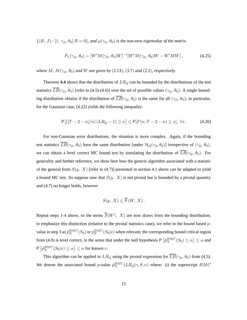
This algorithm can be applied toLRQ using the pivotal expression forLR(γ0, θ0) from (4.5).

We denote the associated boundp-value pBMCN (LRQ|γ, θ, ν) where: (i) the superscriptBMC

15

[rather thanPMC as in (4.10)] indicates that the MCp-value is bound-based, (ii)ν refers to the

parameter of the error distribution which is for the moment considered known, and (iii) conditioning

on γ andθ identifies the specific choice forγ andθ underlying the bound. This emphasizes that

invariance of the bounding distributions generated byLR(γ0, θ0) may not necessarily hold. In this

case, numerical methods may be needed to evaluate the boundsin (4.23)-(4.24). So it is not clear

that this is any simpler than drawing the setC(α; γ, θ) using numerical methods. However, even

then, a useful bound may still be obtained by considering thesimulated distribution obtained on

replacing(γ0, θ0) by their QMLE estimates inLR(γ0, θ0), where the estimates are treated as fixed

known parameters. This yields the following boundp-value:

pBMCN (γQ, θQ, ν) ≡ pBMC

N (LRQ|γQ, θQ, ν). (4.27)

Then, we have the following implication:

pBMCN (LRQ|γQ, θQ, ν) > α ⇒ pPMC

N [LR(γ0, θ0)|ν] > α , for some(γ0, θ0). (4.28)

In other words, ifpBMCN (LRQ|γQ, θQ, ν) > α, we can be sure thatC(α; γ, θ) is not emptyso that

HQ is not rejected by the test in (4.14).

4.3. A bootstrap-type LR test

With N draws from the distribution ofW1, . . . , WT , N simulated samples can be constructed con-

formably with (2.7)-(2.9), (2.2) under the null hypothesis (2.5), given any value for{B,Σ} ∈ ΨQ

whereΨQ refers to the parameter space compatible with the null hypothesisHQ. Applying (3.19)

to each of these samples yieldsN simulated statistics from the null data generating process.

Count the number of simulated statistics≥ {observedLRQ} and replace this number forGN (.)

in (4.8); this provides a MCp-value conditional on the choice forB and Σ which we denote

pLMCN (LRQ|B,Σ, ν) where the symbol LMC stands forLocal MC to emphasize that it is esti-

mated given a specific nuisance parameter value. In particular, it is natural to consider the QMLE

16

estimatesBQ andΣQ defined in (3.20) which yields

pLMCN (BQ, ΣQ, ν) ≡ pLMC

N (LRQ|BQ, ΣQ, ν). (4.29)

This bootstrap-typep-value differs from the bound-basedp-value pBMCN (LRQ|γQ, θQ, ν) from

(4.27), although both use QMLE estimates. Indeed, as a consequence of Theorem4.4, it is straight-

forward to see thatpBMCN (LRQ|γQ, θQ, ν) ≥ pLMC

N (LRQ|BQ, ΣQ, ν). Relying on the latter will

not necessarily yield a level correct test in finite samples.However, since

pLMCN (LRQ|BQ, ΣQ, ν) > α ⇒ sup

{B,Σ}∈ΨQ

pLMCN (LRBCAPM |B,Σ, ν) > α

whereB,Σ refer to the parameter space compatible with the null hypothesis. So a non-rejection

based onpLMCN (LRQ|BQ, ΣQ, ν) can be considered conclusive from an exact test perspective.

5. The case of error distributions with unknown parameters

We will now extend the above results to the unknown distributional parameter case for the error

families of particular interest, namely (2.2). To do this, it is helpful to first revisit the generic

algorithm and its modification presented in sections 4.1 and4.2 above. The outcome of the both

algorithms, namely thep-valuespPMCN (S0|ν) andpBMC

N (S0|ν) are valid ifν is known. Whenν is

unknown, we can apply the method of maximized Monte Carlo (MMC) tests [see Dufour (2006)] to

obtain tests that satisfy the level constraint even in finitesamples: given a set of nuisance parameters

Φ0 consistent with the null hypothesis of interest, the critical regions

supν ∈ Φ0

[pPMCN (S0|ν)] ≤ α, sup

ν ∈ Φ0

[pBMCN (S0|ν)] ≤ α. (5.1)

have levelα. This suggests to maximize the MCp-values presented in sections 4.1, 4.2 and 4.3

above. Rather than consideringΦ0 as a search set, we focus on a set estimate forν [see e.g. Dufour

and Kiviet (1996) and Beaulieu, Dufour and Khalaf (2005, 2006, 2007)] to ensure that the error

17

distributions retained are empirically relevant. Formally, we consider the following critical regions:

QBMCU (γ, θ) ≤ α2 , QBMC

U (γQ, θQ) ≤ α2 , (5.2)

QBMCU (γQ, θQ) = sup

ν ∈ C(Y )pBMC

N (LRQ|γQ, θQ, ν), (5.3)

QLMCU (BQ, ΣQ) = sup

ν∈ C(Y )pLMC

N (LRQ|BQ, ΣQ, ν) (5.4)

wherepBMCN (LRQ|γQ, θQ, ν) [defined in (4.27)] is the specific bound based on QMLE estimates

of γ and θ, pLMCN (LRQ|BQ, ΣQ, ν) [defined in (4.29)] is the LMC bootstrap-typep-value, and

C(Y ) is an(1-α1) level confidence set forν [described below]. Non-rejections [refer to sections 4.2

and 4.3] based on (5.2) are exact at theα1 + α2 level. In section 8, we useα1 = α2 = α/2.

To obtainC(Y ), we “invert” a test for hypothesis (2.2) whereν = ν0 and knownν0. Inverting an

α1 level test involves collecting the values ofν0 not rejected by this test at levelα1. We consider a

test which assesses lack-of-fit of the hypothesized distribution. In what follows, we briefly describe

this test; for more complete algorithms, proofs and references, see Dufour, Khalaf and Beaulieu

(2003) and Beaulieu et al. (2007). We consider

ESK(ν0) =∣

∣SK−SK(ν0)∣

∣ , EKU(ν0) =∣

∣KU−KU(ν0)∣

∣ , (5.5)

whereSK andKU are the multivariate skewness and kurtosis criteria

SK =1

T 2

T∑

t=1

T∑

i=1

d3ii, KU =

1

T

T∑

t=1

d2tt, (5.6)

dit are the elements of the matrixU(U ′U)−1U ′, andSK(ν0) andKU(ν0) are simulation-based es-

timates of the expectedSK andKU given (2.2). These are obtained, givenν0, by drawing samples

conformable with (2.2) then computing the corresponding average measures of skewness and kur-

tosis. The MC test technique may be applied to obtain exactp-values forESK(ν0) andEKU(ν0)

as follows. Conditional on the sameSK(ν0) andKU(ν0), generate, imposingν = ν0, replica-

tions of the excess skewness and excess kurtosis statistics. Exact Monte Carlop-values [denoted

18

p(ESK0 |ν0) and p(EKU0 |ν0)] for each test statistic can be calculated from the rank of the ob-

servedESK(ν0) andEKU(ν0) relative to the simulated ones. The generic algorithm presented in

section 4.1 also applies here, where the relevant pivotal characterizations can be found in Dufour

et al. (2003). To obtain a joint test based onSK andKU, we consider the joint criterion:

CSK = 1 − min {p(ESK0 |ν0), p(EKU0 |ν0)} . (5.7)

The MC test technique is once again applied to obtain a size correctp-value for the combined test.

6. A less restricted model

We now turn to the general hypothesis (2.14). Let us first observe that the hypothesis may be re-

written in matrix formHGQMM : [1, γ, θ]B = φι′n, whereιn is ann-dimensional vector of ones.

If φ is known, then it is possible to use the above eigenvalue testprocedure to derive its associated

LR statistic. One maye.g.consider the MLR:

Rit − RMt − φ = ai + (bi − 1)RMt + ciR2Mt + uit, t = 1, . . . , T, i = 1, . . . , n. (6.8)

In this context, testingHGQMM corresponds to assessing

ai + γ(bi − 1) + ciθ = 0, i = 1, . . . , n, (6.9)

which leads to the above framework. This also suggests a simple procedure to derive the LR statistic

to testHGQMM and the associated MLE estimate ofφ. Indeed, one may minimize, overφ, the

eigenvalue based criterion associated with (6.8)-(6.9); this may be conducted numerically (yet since

the argument of the underlying minimization is scalar, thisapproach is numerically much more

tractable than the iterative maximization applied by Barone-Adesi et al. (2004b)). The statistical

solutions we derived above also hold in this framework: indeed, bounding cut-off points can be

obtained using the null distribution of the test statistic which fixesφ to a known value. Note however

that we have shown in Dufour and Khalaf (2002) that the latterdistribution does not depend onφ,

19

which will lead one to the same bound whetherφ is zero or not. Tighter bounds can be obtained

under normality; see Velu and Zhou (1999) or Zhou (1995).

7. Simulation study

We now present a small-scale simulation experiment to assess the performance of the proposed tests.

We focus onHQ [hypothesis (2.5)] in the context of (2.1). The design is calibrated to match our

empirical analysis (see section 8) which relies on monthly returns of 25 value-weighted portfolios

from Fama and French’s data base, for 1961-2000. Since we assess the model over 5-year intervals

(as well as over the whole sample), we consider (2.1) withn = 25 equations andT = 60, which

reflect our subperiod analysis.RMt, t = 1, ..., T are fixed to the returns on the market portfolio from

the aforementioned data set for the 1996-2000 time period. The coefficients of this regressor and its

square, namelybi andci, i = 1, . . . , n, in (2.1), are fixed to their observed counterparts, namely,

bi and ci, i = 1, . . . , n, corresponding to the unconstrained OLS regression over the 1996-2000

sample period; from this same regression, we also retain: (i) the largest intercept estimate

a = maxi

{ai} , i = 1, . . . , n, (7.1)

to set the scale for the power study (see below), and (ii) the estimated variance-covariance error

matrix, to generate model shocks; formally, we use (2.2) substituting the Cholesky factor of the

variance-covariance estimate in question for theJ matrix.

We study normal andt-errors with unknown degrees-of-freedom, so the random errors Wt,

t = 1, ..., T in (2.2) are generated as in (2.3) and (2.4), respectively. In the latter case, the degrees-

of-freedom parameterκ is fixed to8. This choice is also motivated by our empirical application: as

may be checked from Table 4 in section 8, the average lower limit of the confidence set forκ over

the eight 5-year subperiods analyzed is around 8. The MC tests are applied imposing and ignoring

information onκ, which allows to document the cost of estimating this parameter. Whenκ is taken

as unknown, MMCp-values are calculated over the space4 ≤ κ ≤ 13. A wider range is allowed

in our empirical application; in the case of the simulation study, this restriction is adopted to keep

20

execution time manageable.

Several choices for the key parametersγ andθ are evaluated, particularly to assess the size of

asymptotic tests. Again, we rely on the data set analyzed in the next section, as follows. We consider,

in turn, the QMLE estimates ofγ andθ from each of the eight 5-year sub-samples analyzed; we

also consider an alternative design settingγ andθ to the average of their estimates over the eight

5-year subperiods. The latter design is used for the power study (see below).

We study the LR statistic defined in the previous sections, with its asymptoticχ2 p-value, its

QMLE-based boundp-value and its QMLE-based bootstrap typep-value.

The model intercepts are set as follows. For the size study,HQ [hypothesis (2.5)] is imposed so

ai, i = 1, . . . , n, are obtained given the choices forbi andci, andγ andθ described above. For

the power study, intercepts are generated such that

ai = −γ(bi − 1) − ciθ + ∆ a, i = 1, . . . , n, (7.2)

wherea is defined in (7.1) and∆ is a scalar ranging from0.25 to 2.5 which controls the extent of

departure fromHQ; clearly,∆ = 0 yieldsHQ. Here again, the constanta aims at calibrating the

design to our empirical application, for empirical relevance purposes.

In all designs,N = 99 replications are used to implement MC tests [we used 999 in the em-

pirical application]. The literature on MC testing [seee.g. Dufour and Kiviet (1996), Dufour and

Khalaf (2002) or Dufour, Khalaf, Bernard and Genest (2004)]illustrates reliability withN = 99

in simulation studies. In each experiment, the number of simulations is 1000; we report empirical

rejections for a nominal level of5%.

Results reveal that theχ2 asymptotic test is oversized for all designs considered; indeed, em-

pirical sizes range from a minimum of 25.8% to 32.3%. Since wehave attempted to calibrate

simulation designs to the empirical study, these results confirm our reliance on MC alternatives to

the usual asymptotic cut-off points. It is worth noting thatover-rejections with normal errors are

almost as severe as with the Student-t case. To interpret the bootstrap results in Table 1, recall

that for the Student-t distribution, the degrees-of-freedom are assumed known (this assumption is

relaxed in Table 2), whereas all remaining nuisance parameters are estimated consistently under the

21

Table 1. Size of asymptotic and parametric bootstrap QMM tests

(1) (2) (3) (4) (5) (6) (7) (8)

Normal Asy .287 .291 .279 .295 296 .275 .258 .287LMC .062 .062 .051 .087 .072 .039 .029 .077

Student-t Asy .314 .313 .317 .300 .314 .323 .288 .319LMC [ κ known] .073 .074 .069 .087 .077 .062 .029 .109

Note – Numbers shown are empirical rejections for proposed tests ofHQ [hypothesis (2.5) in the context of (2.1)]. Thestatistic considered is the quasi-LR statistic (3.19); associatedp-values rely on, respectively, the asymptoticχ2(n − 2)distribution and the LMCp-values assuming the error distribution is known, which corresponds to a parametric bootstrap.Columns (1) - (8) refer to the choices for the parametersγ andθ underlying the various simulation designs considered.These parameters are fixed, in turn, to their QMLE counterparts based on the data set analyzed in section 8, over eachof the eight 5-year subperiods under study, so column (1) refers to parameters estimated using the 1961-65 subsample,column (2) to the 1966-70 subsample, etc.

null hypothesis. Bootstrapping reduces over-rejections so tests based on LMCp-values deviate only

moderately from their nominal size: rejection probabilities range from 2.9% to 8.7% with normal

errors and from 2.9% to 10.9% with Student-t errors.

Results of the power study reported in Table 2 show that the tests have a good power perfor-

mance. Observe that empirical rejections associated with∆ 6= 0 in columns (1) and (4) of Table

2 convey a misleading assessment of power, since the underlying χ2-based tests are severely over-

sized. In such cases, a size-correction scheme is required;for instance, one may compute an artificial

size-correct cut-off point from the quantiles of the simulated statistics conditional on each design.

Since the bootstrap-type correction seems to work, at leastlocally, for the design under study, we

prefer to analyze the bootstrap version of the tests rather than resorting to another artificial size

correction. Indeed, whereas bootstrap-based size corrections are empirically applicable, a local cor-

rection corresponds to a practically infeasible test. Though simulation results generally depend on

the designs considered, the following findings summarized next are worth noting.

1. Estimation costs for the degrees-of-freedom parameter with Student-t errors are unnoticeable.

Indeed, the empirical rejections based onBMC p-values are identical whetherκ is treated

as a known or as an unknown scalar. The bootstrap typeLMC tests are affected albeit

moderately from estimatingκ.

22

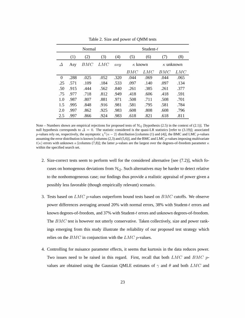
Table 2. Size and power of QMM tests

Normal Student-t

(1) (2) (3) (4) (5) (6) (7) (8)

∆ Asy BMC LMC asy κ known κ unknown

BMC LMC BMC LMC

0 .288 .025 .052 .320 .044 .069 .044 .065.25 .571 .109 .184 .533 .097 .140 .097 .134.50 .915 .444 .562 .840 .261 .385 .261 .377.75 .977 .718 .812 .949 .418 .606 .418 .5911.0 .987 .807 .881 .971 .508 .711 .508 .7011.5 .995 .848 .916 .981 .581 .795 .581 .7842.0 .997 .862 .925 .983 .608 .808 .608 .7962.5 .997 .866 .924 .983 .618 .821 .618 .811

Note – Numbers shown are empirical rejections for proposed tests ofHQ [hypothesis (2.5) in the context of (2.1)]. Thenull hypothesis corresponds to∆ = 0. The statistic considered is the quasi-LR statistics [refer to (3.19)]; associatedp-values rely on, respectively, the asymptoticχ2(n − 2) distribution [columns (1) and (4)], the BMC and LMCp-valuesassuming the error distribution is known [columns (2,3) and(5,6)], and the BMC and LMCp-values imposing multivariatet(κ) errors with unknownκ [columns (7,8)]; the latterp-values are the largest over the degrees-of-freedom parameter κ

within the specified search set.

2. Size-correct tests seem to perform well for the considered alternative [see (7.2)], which fo-

cuses on homogenous deviations fromHQ. Such alternatives may be harder to detect relative

to the nonhomogeneous case; our findings thus provide a realistic appraisal of power given a

possibly less favorable (though empirically relevant) scenario.

3. Tests based onLMC p-values outperform bound tests based onBMC cutoffs. We observe

power differences averaging around 20% with normal errors,38% with Student-t errors and

known degrees-of-freedom, and 37% with Student-t errors and unknown degrees-of-freedom.

TheBMC test is however not utterly conservative. Taken collectively, size and power rank-

ings emerging from this study illustrate the reliability ofour proposed test strategy which

relies on theBMC in conjunction with theLMC p-values.

4. Controlling for nuisance parameter effects, it seems that kurtosis in the data reduces power.

Two issues need to be raised in this regard. First, recall that both LMC and BMC p-

values are obtained using the Gaussian QMLE estimates ofγ and θ and bothLMC and

23

BMC procedures are not invariant to the latter. In addition, thetest statistic is based on

Gaussian-QMLE, although we have corrected its critical region for departures from normal-

ity. Gaussian-QMLE coincides with least squares in this model, and least-squares-based sta-

tistics are valid (although possibly not optimal) in non-normal settings, at least in principle.

We view our results as a motivation for research on finite-sample robust test procedures in

MLR models.

8. Empirical analysis

For our empirical analysis, we use Fama and French’s data base. We produce results for monthly

returns of 25 value-weighted portfolios from 1961-2000. The portfolios which are constructed at the

end of June, are the intersections of five portfolios formed on size (market equity) and five portfolios

formed on the ratio of book equity to market equity. The size breakpoints for years are the New

York Stock Exchange (NYSE) market equity quintiles at the end of June of years. The ratio of

book equity to market equity for June of years is the book equity for the last fiscal year end ins−1

divided by market equity for December of years− 1. The ratio of book equity to market equity are

NYSE quintiles. The portfolios for July of years to June of years + 1 include all NYSE, AMEX,

NASDAQ stocks for which we have market equity data for December of years−1 and June of year

s, and (positive) book equity data fors − 1. All MC tests where applied with 999 replications, and

multivariate normal and multivariate Student-t errors; formally, as in (2.3) and (2.4) respectively.

Table 3 reports tests ofHQ [hypothesis (2.5) in the context of (2.1)] and ofHGQMM [hypothesis

(2.14) in the context of (2.1)], over intervals of 5 years andover the whole sample. Subperiod

analysis is usual in this literature [seee.g. the surveys of Black (1993) or Fama and French (2004)],

and is mainly motivated by structural stability arguments.Our previous and ongoing work on related

asset pricing applications [Beaulieu, Dufour and Khalaf (2005, 2006, 2007), Dufour, Khalaf and

Beaulieu (2008)] have revealed significant temporal instabilities which support subperiod analysis

even in conditional models which allow for time varyingbetas.

To validate our statistical setting, companion diagnostictests are run and are reported in Table

4. These include: (i) goodness of fit tests associated with distributional hypotheses (2.3) and (2.4);

24

Table 3. QMM and GQMM tests

Tests ofHQ Tests ofHGQMM

(1) (2) (3) (4) (5) (6) (7) (8) (9) (10)

Sample Asy pBMCN pLMC

N pBMCt

pLMCt

Asy pBMCN pLMC

N pBMCt

pLMCt

1961-1965 .078 .586 .405 .596 .414 .099 .666 .468 .678 .4741966-1970 .008 .246 .134 .255 .143 .217 .813 .646 .828 .6521971-1975 .054 .515 .341 .529 .367 .227 .815 .664 .828 .6741976-1980 .000 .006 .002 .015 .006 .215 .793 .670 .810 .6791981-1985 .001 .081 .022 .093 .033 .002 .133 .061 .176 .0851986-1990 .003 .163 .074 .193 .091 .029 .448 .283 .467 .2951991-1995 .001 .114 .055 .148 .076 .002 .163 .071 .196 .0961996-2000 .073 .543 .386 .591 .420 .229 .803 .665 .830 .677

1961-2000 .000 .001 .001 .002 .002 .003 .011 .015 .002 .005

Note – Columns (1)-(5) pertain to tests ofHQ [hypothesis (2.5) in the context of (2.1)]; columns (6)-(10) pertain to tests ofHGQMM [hypothesis (2.14) in the context of (2.1)]. Numbers shown arep-values, associated with the quasi-LR statistics[refer to (3.19)], relying on, respectively, the asymptotic χ2(n−2) distribution [columns (1) and (6)], the Gaussian basedBMC and LMC p-values [columns (2)-(3) and (7)-(8)], and the BMC and LMCp-values imposing multivariatet(κ)errors [columns (4)-(5) and (9)-(10)]. MCp-values fort(κ) errors are the largest over the degrees-of-freedom parameterκ within the specified confidence sets; the latter is reported in column 6 of Table 4. January and October 1987 returns areexcluded from the dataset.

(ii) tests for departure from the maintained errori.i.d. hypothesis, and (iii) tests for exogeneity of

the market factors.

The goodness-of-fit tests rely on the multivariate skewness-kurtosis criteria described in section

5. For the normal distribution, we apply the pivotal MC procedure to the omnibus statistic:

MN =T

6SK+

T [KU−n(n + 2)]2

8n(n + 2). (8.1)

For the Student-t distribution, we report the confidence set for the degrees-of-freedom parameter

which inverts the combined skewness-kurtosis statistic (5.7).

Serial dependence tests [from Dufour et al. (2008) and Beaulieu et al. (2007)] are summarized

here for convenience. In particular, we apply the LM-GARCH test statistic [Engle (1982)] and

the variance ratio statistic which assesses linear serial dependence [Lo and MacKinlay (1988)], to

25

standardized residuals, namelyWit, the elements of the matrix

W = U S−1

U, (8.2)

whereSU is the Cholesky factor ofU ′U . So the modified GARCH test statistic for equationi,

denotedEi, is given byT× (the coefficient of determination in the regression of the equation’s

squared OLS residualsW 2it on a constant andW 2

(t−j),i , j = 1, . . . , q) whereq is the ARCH order

against which the test is designed. The modified variance ratio is given by:

˜V Ri = 1 + 2K

∑

j=1

(

1 −j

K

)

ρij , ρij =

∑Tt=j+1 WitWi,t−j

∑Tt=1 W 2

ti

. (8.3)

12 lags are used for both procedures. We combine inference across equation via the joint statistics:

E = 1 − min1≤i≤n

[

p(Ei)]

, ˜V R = 1 − min1≤i≤n

[

p( ˜V Ri)]

, (8.4)

wherep(Ei) andp( ˜V Ri) refer top-values, obtained using theχ2(q) andN[

1, 2(2K − 1)(K −

1)/(3K)]

respectively. In Dufour et al. (2008), we show that under (2.2), W has a distribution

which depends only onκ, so the MC test technique can be applied to obtain a size correct p-value

for E and ˜V R. To deal with an unknownκ, we apply an MMC test procedure following the same

technique proposed for tests onHQ. Specifically, we use the same confidence set forκ, of level

(1 − α1); we maximize thep-value function associated withE and ˜V R over all values ofκ in the

latter confidence set; we then refer the latter maximalp-value toα2 whereα = α1 + α2. Power

properties of these tests are analyzed in Dufour et al. (2008) and suggest a good performance for

sample sizes compatible with our subperiod analysis.

We also apply the Wu-Hausman test to assess the potential endogeneity of our regressors. It

consists in appending, to each equation, the residuals froma first stage regression of returns on a

constant and the instruments, and testing for the exclusionof these residuals using the usual OLS

basedF-statistic [see Hausman (1978), Dufour (1987)]. This test is run, in turn, for each equation,

with one lag ofRM , R2M andRi, i = 1, 25 as instruments. Numbers shown are the minimum

26

p-values over all equations. The usualF-basedp-value is computed for the normal case; for the

Student-t, we compute MMCp-values, as follows. In each equation, and ignoring contemporaneous

correlation of the error term, theF-statistic in question is location-scale invariant and caneasily

be simulated to derive a MCp-value given draws from a Student-t distribution, conditional on

its degrees-of-freedom. We maximize thep-value so obtained overκ in the same confidence set

used for all other tests as described above; we then refer thelatter maximalp-value toα2 where

α = α1 + α2. For presentation clarity, we report the minimump-value in each case, over all

equations.

For all confidence set based MMC tests under the Student-t hypothesis, we considerα1 = 2.5%

so, in interpreting thep-values reported in following tables for the Student-t case,α1 must be

subtracted from the adopted significance level; for instance, to obtain a5% test, reportedp-values

should be referred to 2.5% as a cut-off.

From Table 3, we see that, when assessed using the whole sample, bothHQ andHGQMM are

soundly rejected, using asymptotic or MCp-values, the confidence sets on the degrees-of-freedom

parameter is quite tight and suggests high kurtosis, and normality is definitely rejected. Unfortu-

nately, the diagnostic tests (Table 4) reveal significant departures from the statistical foundations

underlying the latter tests (even when allowing for non-normal errors); temporal instabilities thus

cast doubt on the full sample analysis.

Results over subperiods can be summarized as follows. Multivariate normality is rejected in

many subperiods and provides us with a reason to investigatewhether test results shown under

multivariate normality are still prevalent once we use Student-t distributions. HQ is rejected at

the 5% level in five subperiods out of eight using asymptoticp-values. Using finite-sample tests

under multivariate normality reveals thatHQ is rejected at the5% level in only one subperiod,

namely 1976-1980. The LMCp-value confirms all these non-rejections but one. Using the same

approach under the multivariate Student-t distribution leads to the same conclusion.HGQMM is not

rejected in any subperiod allowing fort-errors, although the normal LMCp-value is less than5% for

1986-90, and asymptoticp-values are highly significant for three subperiods spanning 1981-1995.

Diagnostic tests allowing fort errors reveal significant (at the5% level) departures from thei.i.d.

27

Table 4. Multivariate diagnostics

Time Dependence Goodness-of-fit Exogeneity

E ˜V R MN CS(κ) Wu-Hausman

(1) (2) (3) (4) (5) (6) (7) (8)

Sample Normal Student-t Normal Student-t Normal Student-t Normal Student-t

1961-1965 .718 .769 .117 .135 .026 ≥ 8 .214 .2351966-1970 .258 .314 .954 .996 .044 ≥ 8 .079 .1001971-1975 .215 .266 .253 .260 .015 ≥ 7 .018 .0261976-1980 .001 .004 .502 .516 .004 ≥ 6 .003 .0051981-1985 .222 .237 .131 .148 .001 ≥ 5 .143 .1611986-1990 .544 .559 .056 .070 .401 ≥ 12 .042 .0531991-1995 .150 .166 .142 .149 .176 ≥ 9 .259 .2851996-2000 .010 .049 .847 .849 .001 3 − 11 .194 .189

1961-2000 .001 .001 .002 .007 .001 5 − 8 .000 .001

Note – Numbers shown in columns (1)-(5) and (7)-(10) arep-values associated with the combined test statisticsE

[columns (1) and (2)], ˜V R [columns (3) and (4)],MN [column (5)] andWH [columns (7)-(10)].E, defined by (8.4),

is a multivariate extension of Engle’s GARCH test statistic. ˜V R, defined by (8.4), is a multivariate extension of Lo

and MacKinlay’s variance ratio test.MN is a MC version of the multivariate combined skewness and kurtosis test

based on (8.1). The Wu-Hausman test is applied with one lag ofRM , R2

M andRi, i = 1, 25 as instruments. Numbers

shown are the minimump-values over all equations; the usualF-basedp-value is computed for the normal case; for

the Student-t, we compute MMCp-values. Both normal and Student-t p-values for this test are univariate. In columns

(1), (3), (5) and (7), the Gaussianp-values are MC pivotal statistics based;p-values in columns (2), (4), (6) and (8)

are MMC confidence set based; the relevant 2.5% confidence set for the nuisance parameters is reported in column (6).

Specifically,CS(κ) corresponds to the confidence set estimate of level97.5% for the degrees-of-freedom parameter of

the multivariate Student-t error distribution; this set is obtained by inverting the goodness-of-fit statistic (5.7).

hypothesis in the 1976-1980 subperiod and not elsewhere. Recall that in this same subperiod, our

QLR tests rejectHQ at the5% level.

We conclude by underlying the evidence that contrary to the asset pricing evidence in the lit-

erature, this version of the CAPM is generally not rejected by our tests, even when controlling

for finite-sample inference. Compared to the results of Beaulieu, Dufour and Khalaf (2005, 2006,

2007), we see that the QMM model is not rejected using our tests, whereas both Black’s version of

the CAPM, or the CAPM with observed risk-free rate are rejected using related test methods. This

observation must be qualified since the diagnostic tests applied to the overall sample are significant

at conventional levels revealing temporal instabilities.Care must be exercised in interpreting our

28

generalized Wu-Hausman test results. Indeed, recall that the reportedp-values are the smallest over

all equations, and thep-values (including the simulated ones), are univariate, inthe sense that con-

temporaneous correlation of shocks is ignored. If we consider a Bonferroni approach to obtain a

valid joint test, which involves dividing the adopted test level by 25 here, we see that for the full

sample, the test remains significant even with such a conservative correction. This result may be

viewed as a motivation for conditional three-moment based modeling.

9. Conclusion

In this paper, we consider the quadratic market model which extends the standard CAPM framework

to incorporate the effect of asymmetry of return distribution on asset valuation. The development

of exact tests of the QMM is an appealing research objective,given: (i) the increasing popularity of

this model in finance, (ii) the fact that traditional market models (which suppose that asset returns

move proportionally to the market) have not fared well in empirical tests, (iii) available related

studies are only asymptotic (exact tests are unavailable even with normal errors). We have proposed

exacts tests of the QMM allowing for non-normal distributions exactly. The underlying statistical

challenges relate to dimensionality tests which are interesting in their own right. Our results show

that although asymptotic tests are significant in several subperiods, exact tests fail to reject this

model with Fama-French data. Temporal instabilities are however evident, and motivate exploring

conditional three-moment based models.

29

References

Barone-Adesi, G. (1985), ‘Arbitrage equilibrium with skewed asset returns’,Journal of Financial

and Quantitative Analysis20(3), 299–313.

Barone-Adesi, G., Gagliardini, P. and Urga, G. (2004a), A test of the homogeneity hypothesis on

asset pricing models,in E. Jurczenko and B. Maillett, eds, ‘Multi-Moment CAPM and Related

Topics’, Springer-Verlag, Berlin.

Barone-Adesi, G., Gagliardini, P. and Urga, G. (2004b), ‘Testing asset pricing models with coskew-

ness’,Journal of Business and Economic Statistics22(4), 474–485.

Beaulieu, M.-C., Dufour, J.-M. and Khalaf, L. (2005), Exactmultivariate tests of asset pricing

models with stable asymmetric distributions,in M. Breton and H. Ben Ameur, eds, ‘Numerical

Methods in Finance’, Kluwer/Springer-Verlag, New York, chapter 9, pp. 173–191.

Beaulieu, M.-C., Dufour, J.-M. and Khalaf, L. (2006), Testing Black’s CAPM with possibly non-

gaussian errors: An exact identification-robust simulation-based approach, Technical report,

CIREQ, Université de Montréal and Université Laval.

Beaulieu, M.-C., Dufour, J.-M. and Khalaf, L. (2007), ‘Multivariate tests of mean-variance effi-

ciency with possibly non-Gaussian errors: An exact simulation-based approach’,Journal of

Business and Economic Statistics25(4), 398–410.

Black, F. (1972), ‘Capital market equilibrium with restricted borrowing’, Journal of Business

45, 444–454.

Black, F. (1993), ‘Beta and return’,Journal of Portfolio Management20(1), 8–17.

Bolduc, D., Khalaf, L. and Moyneur, E. (2008), ‘Identification-robust simulation-based inference

in joint discrete/continuous models for energy markets’,Computational Statistics and Data

Analysisforthcoming.

Campbell, J. Y. (2003), ‘Asset pricing at the millennium’,Journal of Finance55, 1515–1567.

30

Campbell, J. Y., Lo, A. W. and MacKinlay, A. C. (1997),The Econometrics of Financial Markets,

Princeton University Press, New Jersey.

Dittmar, R. (2002), ‘Nonlinear pricing kernels, kurtosis preferences and the cross-section of equity

returns’,Journal of Finance57, 369–403.

Dufour, J.-M. (1987), Linear Wald methods for inference on covariances and weak exogeneity tests

in structural equations,in I. B. MacNeill and G. J. Umphrey, eds, ‘Advances in the Statistical

Sciences: Festschrift in Honour of Professor V.M. Joshi’s 70th Birthday. Volume III, Time

Series and Econometric Modelling’, D. Reidel, Dordrecht, The Netherlands, pp. 317–338.

Dufour, J.-M. (1997), ‘Some impossibility theorems in econometrics, with applications to structural

and dynamic models’,Econometrica65, 1365–1389.

Dufour, J.-M. (2003), ‘Identification, weak instruments and statistical inference in econometrics’,

Canadian Journal of Economics36(4), 767–808.

Dufour, J.-M. (2006), ‘Monte Carlo tests with nuisance parameters: A general approach to finite-

sample inference and nonstandard asymptotics in econometrics’, Journal of Econometrics

133(2), 443–477.

Dufour, J.-M. and Khalaf, L. (2002), ‘Simulation based finite and large sample tests in multivariate

regressions’,Journal of Econometrics111(2), 303–322.

Dufour, J.-M., Khalaf, L. and Beaulieu, M.-C. (2003), ‘Exact skewness-kurtosis tests for multivari-

ate normality and goodness-of-fit in multivariate regressions with application to asset pricing

models’,Oxford Bulletin of Economics and Statistics65, 891–906.

Dufour, J.-M., Khalaf, L. and Beaulieu, M.-C. (2008), ‘Multivariate residual-based finite-sample

tests for serial dependence and GARCH with applications to asset pricing models’,Journal of

Applied Econometricsforthcoming.

Dufour, J.-M., Khalaf, L., Bernard, J.-T. and Genest, I. (2004), ‘Simulation-based finite-sample tests

for heteroskedasticity and ARCH effects’,Journal of Econometrics122(2), 317–347.

31

Dufour, J.-M. and Kiviet, J. F. (1996), ‘Exact tests for structural change in first-order dynamic

models’,Journal of Econometrics70, 39–68.

Dufour, J.-M. and Taamouti, M. (2005), ‘Projection-based statistical inference in linear structural

models with possibly weak instruments’,Econometrica73(4), 1351–1365.

Dufour, J.-M. and Taamouti, M. (2007), ‘Further results on projection-based inference in IV regres-

sions with weak, collinear or missing instruments’,Journal of Econometrics139(1), 133–153.

Engle, R. F. (1982), ‘Autoregressive conditional heteroscedasticity with estimates of the variance of

United Kingdom inflation’,Econometrica50(4), 987–1008.

Fama, E. F. and French, K. R. (2004), ‘The Capital Asset Pricing Model: Theory and evidence’,

The Journal of Economic Perspectives18(3), 25–46.

Gibbons, M. R. (1982), ‘Multivariate tests of financial models: A new approach’,Journal of Finan-

cial Economics10, 3–27.

Gouriéroux, C., Monfort, A. and Renault, E. (1993), ‘Tests sur le noyau, l’image et le rang de la

matrice des coefficients d’un modèle linéaire multivarié’,Annales d’Économie et de Statistique

11, 81–111.

Gouriéroux, C., Monfort, A. and Renault, E. (1995), Inference in factor models,in G. S. Mad-

dala, P. C. B. Phillips and T. N. Srinivasan, eds, ‘Advances in Econometrics and Quantitative

Economics’, Blackwell, Oxford, U.K., chapter 13, pp. 311–353.

Harvey, C. R. and Siddique, A. (2000), ‘Conditional skewness in asset pricing tests’,The Journal

of Finance55, 1263–1295.

Hausman, J. (1978), ‘Specification tests in econometrics’,Econometrica46, 1251–1272.

Joseph, A. S. and Kiviet, J. F. (2005), ‘Viewing the relativeefficiency of IV estimators in mod-

els with lagged and instantaneous feedbacks’,Computational Statistics and Data Analysis

49, 417–444.

32

Khalaf, L. and Kichian, M. (2005), ‘Exact tests of the stability of the Phillips curve: The Canadian

case.’,Computational Statistics and Data Analysis49, 445–460.

Kiviet, J. F. and Niemczyk, J. (2007), ‘The asymptotic and finite sample distributions of OLS and

simple IV in simultaneous equations’,Computational Statistics and Data Analysis51, 3296–

3318.

Kraus, A. and Litzenberger, R. (1976), ‘Skewness preference and the valuation of risk assets’,Jour-

nal of Finance31, 1085–1100.

Lo, A. and MacKinlay, C. (1988), ‘Stock prices do not follow random walks: Evidence from a

simple specification test’,Review of Financial Studies1, 41–66.

Shanken, J. (1986), ‘Testing portfolio efficiency when the zero-beta rate is unknown: A note’,

Journal of Finance41, 269–276.

Shanken, J. (1996), Statistical methods in tests of portfolio efficiency: A synthesis,in G. S. Mad-

dala and C. R. Rao, eds, ‘Handbook of Statistics 14: Statistical Methods in Finance’, North-

Holland, Amsterdam, pp. 693–711.

Simaan, Y. (1993), ‘Portfolio selection and asset pricing three parameter framework’,Management

Science5, 568–577.

Smith, D. R. (2007), ‘Conditional coskewness and asset pricing’, Journal of Empirical Finance

41, 91–119.

Stock, J. H., Wright, J. H. and Yogo, M. (2002), ‘A survey of weak instruments and weak iden-

tification in generalized method of moments’,Journal of Business and Economic Statistics

20(4), 518–529.

Velu, R. and Zhou, G. (1999), ‘Testing multi-beta asset pricing models’,Journal of Empirical Fi-

nance6, 219–241.

Zhou, G. (1991), ‘Small sample tests of portfolio efficiency’, Journal of Financial Economics

30, 165–191.

33

Zhou, G. (1995), ‘Small sample rank tests with applicationsto asset pricing’,Journal of Empirical

Finance2, 71–93.

34