Finite ElementAnalysis! - University of...

B. Konh, T. Sorensen, A Trimble 1 of XXME 481 – Fall 2017

Finite Element Analysis!

Senior DesignME481

Fall 2017Dr. Bardia Konh


We perform analysis for:• Deformations and internal forces/stresses

• Temperatures and heat transfer in solids

• Fluid flows (with or without heat transfer)

• Conjugate heat transfer (between solids and fluids)

• etc...

Analysis is the key to effective design


Effective design

• Performs the required task efficiently

• is inexpensive in materials used

• is safe under extreme operating conditions

• can be manufactured inexpensively

• is pleasing/attractive to the eye

• etc...


Analysis means probing into, modeling, simulating nature

Therefore, analysis gives us insight into

the world we live in, and this

Enriches our life

Many great philosophers were

analysts and engineers …


Analysis is performed based upon the laws of mechanics

Mechanics

Solid/structural

mechanics

(Solid/structural

dynamics)

Fluid

mechanics

(Fluid

dynamics)

Thermo

mechanics

(Thermo

dynamics)


Physical problem

(given by a “design”)

Mechanical

model

Improve

model

Change of

physical problem

Solution of

mechanical

model

Interpretation

of results

Refine

analysis

Design

improvement

The process of modeling for analysis


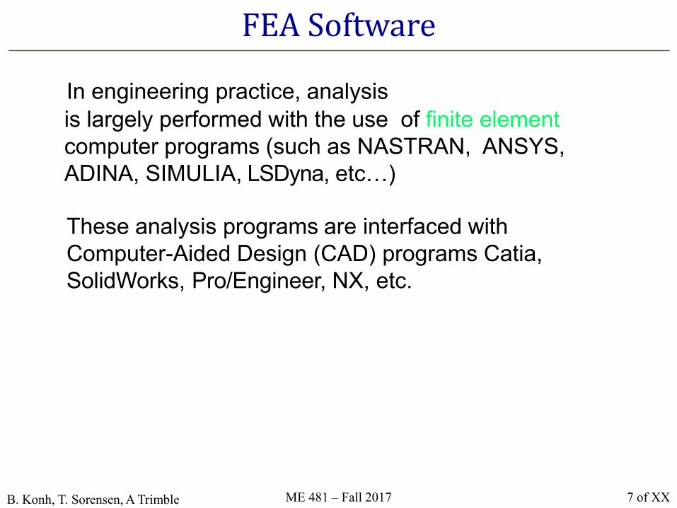
In engineering practice, analysis

is largely performed with the use of finite element

computer programs (such as NASTRAN, ANSYS,

ADINA, SIMULIA, LSDyna, etc…)

These analysis programs are interfaced with

Computer-Aided Design (CAD) programs Catia,

SolidWorks, Pro/Engineer, NX, etc.

FEA Software


Modeling

Means taking increasingly more complex models

to simulate nature with increasing accuracy

Increasingly more

complex models

Assumptions:

spring, rod, truss

beam, shaft

2-D solid

plate

shell

fully three-dimensional

dynamic effects

nonlinear effects

nature


CAD and Analysis

In CAD System

CAD solid model is established

In Analysis System

• Preparation of the mathematical model

• Meshing and Solution

• Presentation of results


Numerical Analyses: Discretization Methods

Nature of Numerical Methods

Consists of a set of numbers from which the distribution of the dependent

variable can be constructed

- Evaluate at any location x, by substituting the values of x and the values of

a's into Equation

- Obtain the values of φ at various locations

- Construct a method that employs the values of φ at a given number of

points (called grid points)

- Conservation of mass, the conservation of momentum, and the

conservation of energy

- a set of algebraic equations for the unknowns

- Prescribing an algorithm for solving the equations

φ = a0 + a1x + a2x2 + · · · + amxm


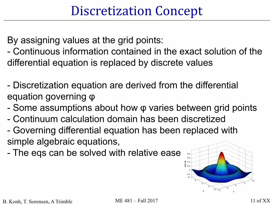
Discretization Concept

By assigning values at the grid points:

- Continuous information contained in the exact solution of the

differential equation is replaced by discrete values

- Discretization equation are derived from the differential

equation governing φ

- Some assumptions about how φ varies between grid points

- Continuum calculation domain has been discretized

- Governing differential equation has been replaced with

simple algebraic equations,

- The eqs can be solved with relative ease


Structure of Discretization Equation

- A discretization equation is an algebraic relation connecting

the values of φ for a group of grid points

- Derived from the differential equation

- With same physical information as the differential equation

- As the number of grid points become very large, the

solution to the discretization equation is expected to

approach the exact solution of the corresponding

differential equation

- Wont give the exact same solution


Finite Element Method

- Whole Domain and Finite element discretization

- Material property (moduli of elasticity for composites) and

geometry vary with spatial coordinate

- Solutions in each of these subdomains are represented by

different functions

- Nodes, elements

- Mesh

- Number of Equations


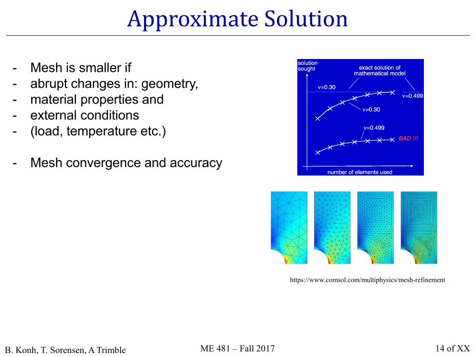
Approximate Solution

- Mesh is smaller if

- abrupt changes in: geometry,

- material properties and

- external conditions

- (load, temperature etc.)

- Mesh convergence and accuracy

https://www.comsol.com/multiphysics/mesh-refinement


Finite Element Representation

http://www.padtinc.com/blog/the-focus/making-pretty-plots-in-

ansys-mechanical-and-mechanical-apdl

http://www.predictiveengineering.com/consulting/ls-dyna-consulting


A reliable and efficient finite element discretization scheme

- for a well-posed mathematical model

- always give,for a reasonable finite element mesh,a reasonable solution

- if the mesh is fine enough, an accurate solution can be obtained


Element Selection

We want elements that are reliable for any

- geometry

- boundary conditions

- and meshing used

The displacement method is not reliable for

- plates and shells

- almost incompressible analysis


Tremendous advances have taken place –

• mixed optimal elements have greatly increased

the efficiency and reliability of analyses

• sparse direct solvers and algebraic multigrid iterative

solvers have lifted the analysis possibilities to completely

new levels

Some analysis experiences


In Industry:Two categories of analyses

• Analysis of problems for which test results are scarce or

non-existent

– large civil engineering structures

• Analysis of problems for which test results can relatively

easily be obtained

– mechanical / electrical engineering structures


Examples of category 1 problems

• Analysis of offshore structures

• Seismic analysis of major bridges

– only "relatively small" components can be tested

Reliable analysis procedures are crucial


Examples of category 2 problems

• Metal forming, crash and crush analyses in the

automobile industries

• These types of problems can now be solved much more

reliably and efficiently than just a few years ago


Reduce Calculation time

- Use symmetry, anti-symmetry, beams, frames, shells, and

trusses

Compare FEA results with mechanics of materials theory

- Analytic approximation

- Then use them to dependently validate a more complex

study

Needle insertion for drug delivery inside a tissue

Fluid-structural analyses

http://uhatmanoa.wixsite.com/ammi/copy-of-smp


Modeling and Optimization of Airbag Helmets for Preventing Head Injuries in Bicycling

Bicycling is the leading cause of sports-related traumatic brain injury (TBI)

Borrowed from Dr. Laksari’s website with permission

M. Kurt, K. Laksari, C. Kuo, G. Grant, D. Camarillo, "Modeling and Optimization of Airbag Helmets for Preventing Head Injuries in

Bicycling", Annals of Biomedical Engineering (2016) [Link].

http://www2.engr.arizona.edu/~klaksari/UA/Brain_Injury.html

http://link.springer.com/article/10.1007/s10439-016-1732-1


Example: Analysis of a Z-section Beam

Z shape cantilever beam

length of L = 500 mm.

thickness of t = 5 mm,

each flange has a length of a = 20 mm,

depth of h = 2a = 40 mm.

loaded by a vertical force P = 500 N


Cantilever Beam

Bending moment, about the x-axis M = P (L – z)

where z is the distance from the support

σz

For symmetric sections: stress is zero at the neutral axis

The load P causes a moment and a shear force

maximum tension along the top edge, and a compression

along the bottom

- Transverse shear stress (τ) varies parabolically through the

depth and has its maximum at the neutral axis


1D Cantilever Beam Theory

Ix is the second moment of inertia

Q is the first moment of the section at a distance, y, from the

neutral axis.

For this section Ix = (2t a3) / 3

The maximum tension will occur at y = a + t/2, while

compression occurs at –y

Uy = PL3 /3EIx = 7.8mm

σz= M y / I

x

τ = P Q /t Ix


3D Beam Theory

The more general non-symmetric beam 1D displacement

predictions are

Uy = - 0.0045, Ux = 0.0067, and Umax = 0.0081 meters

σz = 17.9e7 MPa

Finite ElementAnalysis! - University of...

Documents

Transcript of Finite ElementAnalysis! - University of...