Finite-Element Vibration Analysis and Modal Testing of...

NASA Technical Memorandum 110298U. S. Army Research Laboratory Technical Report 1288

Finite-Element Vibration Analysis and Modal Testing of Graphite Epoxy Tubes and Correlation Between the Data

Barmac K. TaleghaniVehicle Structures DirectorateU.S. Army Research LaboratoryLangley Research Center, Hampton, Virginia

Richard S. PappaLangley Research Center, Hampton, Virginia

November 1996

National Aeronautics andSpace AdministrationLangley Research CenterHampton, Virginia 23681-0001

1

Finite-Element Vibration Analysis and Modal Testing of Graphite Epoxy Tubes and Correlation Between the Data

B. K. Taleghani* and R. S. Pappa**

NASA Langley Research CenterHampton, Virginia

SUMMARY

Structural materials in the form of graphite epoxy composites withembedded rubber layers are being used to reduce vibrations in rocket motortubes. Four filament-wound, graphite epoxy tubes were studied to evaluatethe effects of the rubber layer on the modal parameters (natural vibrationfrequencies, damping, and mode shapes). Tube 1 contained six alternatinglayers of 30-degree helical wraps and 90-degree hoop wraps. Tube 2 wasidentical to tube 1 with the addition of an embedded 0.030-inch-thick rubberlayer. Tubes 3 and 4 were identical to tubes 1 and 2, respectively, with theaddition of a Textron Kelpoxy elastomer. This report compares experimentalmodal parameters obtained by impact testing with analytical modalparameters obtained by NASTRAN finite-element analysis. Four test modesof tube 1 and five test modes of tube 3 correlate highly with correspondinganalytical predictions. Unsatisfactory correlation of test and analysis resultsoccurred for tubes 2 and 4 and these comparisons are not shown. Work isunderway to improve the analytical models of these tubes. Test results clearlyshow that the embedded rubber layers significantly increase structural modaldamping as well as decrease natural vibration frequencies.

--------------------------------------------- * Army Research Laboratory, VSD** NASA Langley Research Center

INTRODUCTION

The Army Research Laboratory’s Vehicle Structures Directorate (ARL, VSD) has a Technology Program Annex (TPA) agreement with theArmy Missile Command (MICOM) to assess the use of layers of rubber toincrease damping in filament-wound, graphite epoxy rocket motor tubes. Thefirst phase of the investigation involves modeling and testing four tubes (twowith a thin rubber layer at the center of the layup and two without the rubberlayer). MICOM fabricated the tubes, performed initial dynamic tests, anddelivered their test results and the four tubes to NASA Langley. Additionaltests were performed at NASA by suspending the tubes from low-frequencysupports, mounting accelerometers, and exciting the tubes with impact loads.Processing the accelerometer responses yielded natural frequencies, mode

2

shapes, and modal damping. The effects of the rubber layer was thenevaluated as was the ability of the analytical models to predict modalcharacteristics of the tubes.

DESCRIPTION OF TEST ARTICLES

The tubes (figure 1) have a 3.6-inch inside diameter, 41-inch length,and wall thicknesses varying from 0.072 inches to 0.102 inches depending onthe layup. The filament winding process used H-IM6 graphite fibers with ananhydride epoxy resin system, wet winding over an aluminum mandrel, andan oven cure in a rotisserie. The cure cycle ramped from an ambientcondition to 300 degrees Fahrenheit and held for three hours to ensurecomplete curing of the matrix. The cylinders were allowed to cool overnightto room temperature, extracted from the mandrel, and then cut to length.

Four tubes (table 1) were manufactured. The baseline tube (tube 1),depicted in figure 2, consisted of alternating layers of 30-degree helical wrapsand 90-degree hoop wraps for a total of six layers. Tube 2 is identical to tube 1with the addition of a 0.030-inch-thick layer of Kevlar-reinforced polyisoprenerubber. The rubber layer was introduced to the cylinder by interrupting thewinding process in the middle of the layup. The rubber layer was hand laid,trimmed, and seamed to provide a uniform thickness. The filament windingprocess was then continued to complete the cylinder fabrication. Tube 3 is thesame as the tube 1 except the epoxy was modified with elastomeric copolymerparticles ranging from 0.01 to 10 microns in diameter. The concentration ofthe spheres in the epoxy was 5 percent by weight. Tube 4 is the same as tube 2except for the addition of an elastomer-modified matrix. The previouslymentioned cure cycle was used for all four tubes.

MODAL TEST METHOD

Figure 1a shows the test configuration. Each tube hung on soft bungeecords to obtain free-free boundary conditions. Figure 3 shows the 4 excitationpositions and 25 accelerometer positions used in each test. Frequencyresponse functions (FRFs) were measured with impact excitation using acommercial “modal testing” hammer; i.e., a hammer with an integral forcegauge. Standard test procedures generated the FRFs with exponentialresponse windowing and 5 ensemble averages. The data-analysis softwareapplied a correction term that removed the increased-damping effects of theexponential window. Each FRF had 512 lines of resolution from 0 to 4096 Hz.

The accelerometer positions used in these tests correspond to thoseused in previous tests performed at MICOM. They adequately measure radialmotion only in the x-z plane passing through the centerline of the tube.Analysis results obtained after testing(discussed in the results section of thereport) show that many more sensors are necessary to fully measure thevibration(modal) characteristics of the tubes up to 2000 Hz.

3

Figure 4 shows sample FRFs for each of the four tubes. These data aredriving-point FRFs of each tube at test point 15Z (i.e., at location 15 in the zdirection). A driving-point FRF is one in which the excitation and responseoccur at the same location and in the same direction. The data are of highquality based on the smoothness of the curves and the regularity of thedriving-point phase angles (always between 0 and 180 degrees). A count of theresonant peaks shows that there are at least 20 modes from 0 to 4096 Hz.

The accelerometer positions used in these tests correspond to thoseused in previous tests performed at MICOM. They adequately measure radialmotion only in x-z plane passing through the centerline of the tube. Analysisresults obtained after testing (discussed in the results section of this report)show that many more sensors are necessary to fully measure the vibration(modal) characteristics of the tubes up to 2000 Hz.

The Eigensystem Realization Algorithm (ERA) (refs. 1 and 2) identifiedstructural modal parameters (natural frequencies, damping, and modeshapes) from the FRFs. ERA is a multiple-input, multiple-output, time-domain technique which analyzes free-decay data or impulse responsefunctions derived by inverse Fourier transformation of FRFs. The FRFs foreach tube were analyzed with ERA in 5 separate analyses as follows: 1) usingall 100 FRFs (4 excitations and 25 responses) simultaneously, 2) using the 25responses for excitation 1X only, 3) using the 25 responses for excitation 15Zonly, 4) using the 25 responses for excitation 17Z only, and 5) using the 25responses for excitation 20Y only. The best result for each mode based on theConsistent-Mode Indicator (CMI) (ref. 1) and visual inspection of modeshapes was selected from among the 5 analyses of each tube.

MODAL AND TRANSIENT RESPONSE ANALYSIS

Finite-Element Model

The MSC/NASTRAN (ref. 3) finite-element model is shown infigure 5. The model consisted of 1312 equally spaced quadrilateral elements,1328 nodes, and 7968 degrees of freedom. The CQUAD4 isoparametricmembrane-bending plate element was used to model the tubes. The modelincorporated 16 elements around the circumference and 83 elements alongthe length. Lumped masses were added as individual point masses located atdesignated nodes of the finite-element model to account for the weight of theinstrumentation (figure 6). As shown in figure 6, 3 triple-axis accelerometers(weighing 22 grams each) were located at the ends of the tube, (b) 15 single-axis accelerometers (weighing 2 grams each) were placed 5 inches apart oneach side of the longitudinal axis of the tubes, and (c) 1 single-axisaccelerometer was located on top. Accelerometers were modeled as pointmasses and were not offset from the structural nodes. The CONM2NASTRAN mass element was used for the point masses.

The Integrated Design Engineering Analysis Software, I-DEAS, (ref. 4)was used for pre-and post-processing. A universal file translator transferred

4

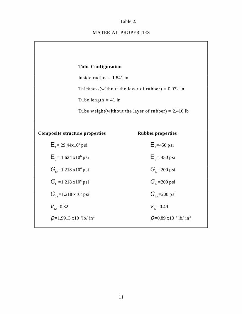
the mesh information into the NASTRAN environment to create the bulkdata deck file for finite-element analysis. Table 2 shows the materialproperties for the analysis. A NASTRAN MAT8 material card definedorthotropic material properties for isoparametric shell elements. Lackingprecise knowledge of the constituent materials, the authors used data givenby Tsai (ref. 5). The density in table 2 is the weight of the tube divided by thevolume of the tube. A separate material card was developed for the layer ofrubber. The rubber properties also appear in table 2.

Eigenvalue Analysis

The analysis of the composite tubes presented here was performedusing version 68 of the MSC/NASTRAN commercial finite-element analysiscomputer code. MSC/NASTRAN Solution Sequence 103 was used to analyzethe model. Mode shapes and frequencies were calculated inMSC/NASTRAN using the Lanczos method (ref. 3). It was decided todetermine all modes with frequencies up to 2000 Hz.

Direct Transient Response Analysis

Transient response analysis allows for studying and optimizing theeffect and the location of the rubber layer within the composite cylinder. Thefollowing result is presented to serve as a baseline for future work oninvestigating the damping effects of the rubber layers in these tubes.

Direct transient response analysis allows the computation of thegeneral dynamic response of a structure. This method performs a numericalintegration on the complete coupled equations of motion, as follows:

M[ ] ˙x{ } + C[ ] x{ } + K[ ] x{ } = f{ } (1)

x x( )00{ } = { }

˙( )x 0 0{ } = { }where:M[ ] = Mass MatrixC[ ] = Damping MatrixK[ ] = Stiffness matrixf{ } = Forcing function˙x{ } = Acceleration vectorx{ } = Velocity vectorx{ } = Displacement vector

x0{ } =Initial displacement vector

5

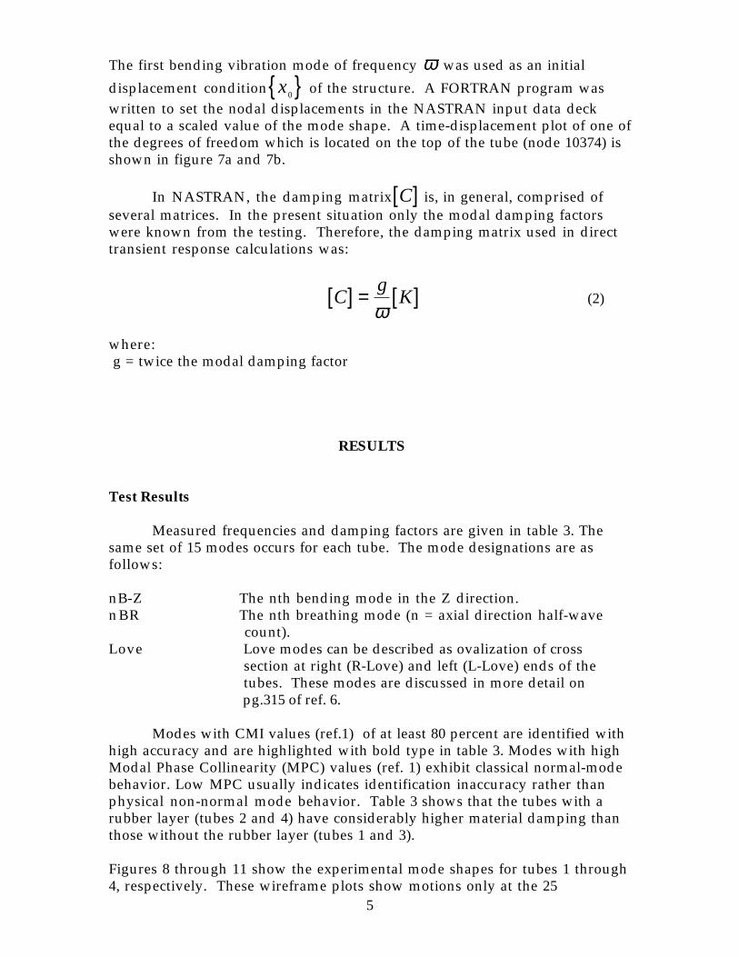
The first bending vibration mode of frequency ω was used as an initial

displacement condition x0{ } of the structure. A FORTRAN program was

written to set the nodal displacements in the NASTRAN input data deckequal to a scaled value of the mode shape. A time-displacement plot of one ofthe degrees of freedom which is located on the top of the tube (node 10374) isshown in figure 7a and 7b.

In NASTRAN, the damping matrix C[ ] is, in general, comprised ofseveral matrices. In the present situation only the modal damping factorswere known from the testing. Therefore, the damping matrix used in directtransient response calculations was:

Cg

K[ ] = [ ]ω

(2)

where: g = twice the modal damping factor

RESULTS

Test Results

Measured frequencies and damping factors are given in table 3. Thesame set of 15 modes occurs for each tube. The mode designations are asfollows:

nB-Z The nth bending mode in the Z direction.nBR The nth breathing mode (n = axial direction half-wave

count).Love Love modes can be described as ovalization of cross

section at right (R-Love) and left (L-Love) ends of the tubes. These modes are discussed in more detail on

pg.315 of ref. 6.

Modes with CMI values (ref.1) of at least 80 percent are identified withhigh accuracy and are highlighted with bold type in table 3. Modes with highModal Phase Collinearity (MPC) values (ref. 1) exhibit classical normal-modebehavior. Low MPC usually indicates identification inaccuracy rather thanphysical non-normal mode behavior. Table 3 shows that the tubes with arubber layer (tubes 2 and 4) have considerably higher material damping thanthose without the rubber layer (tubes 1 and 3).

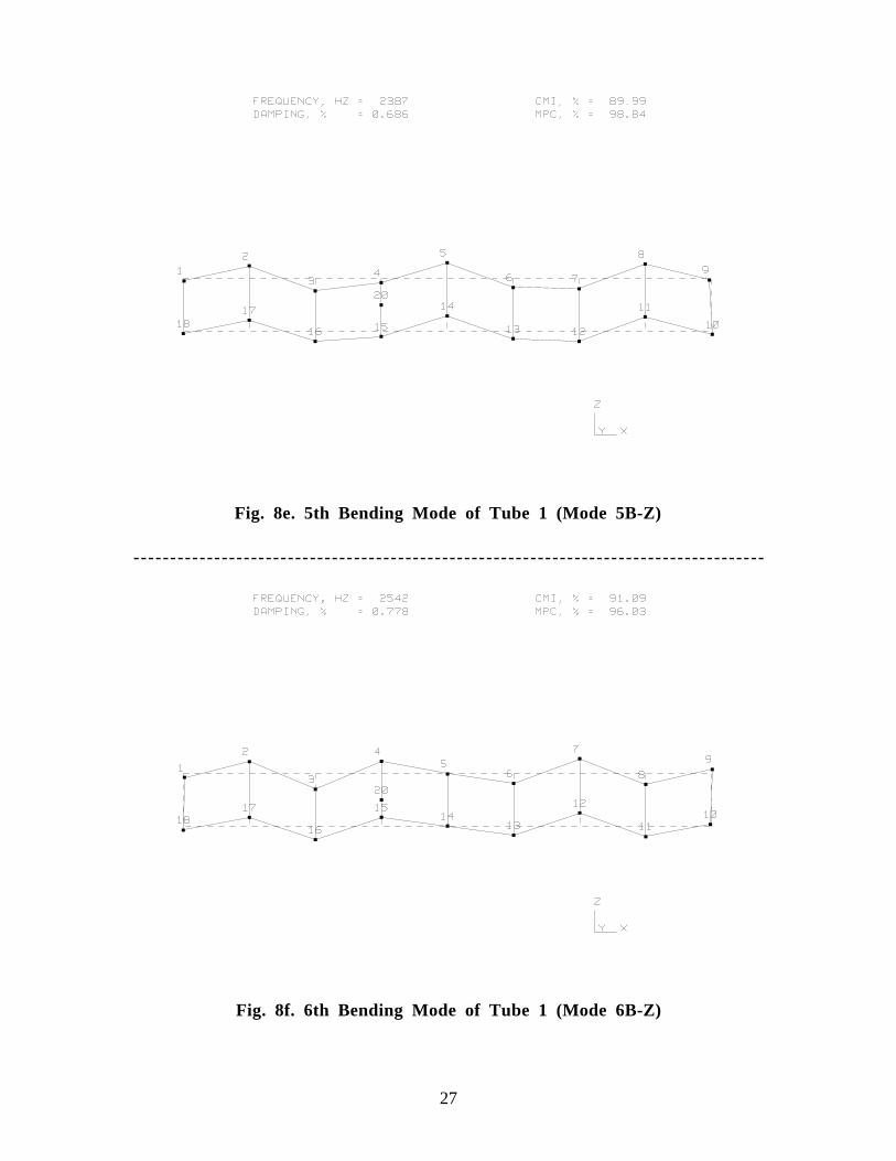
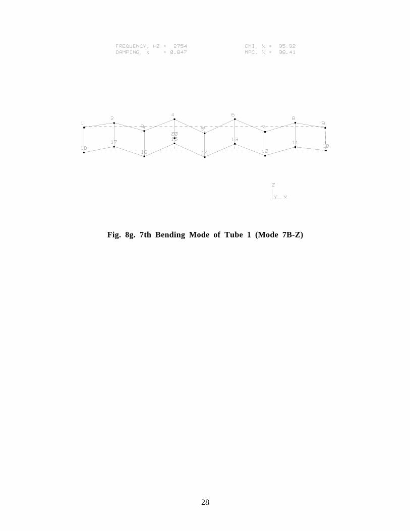
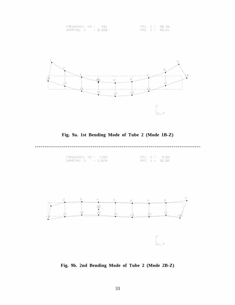
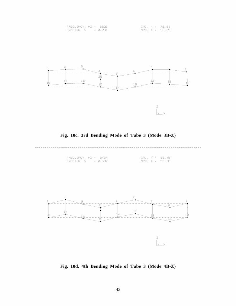
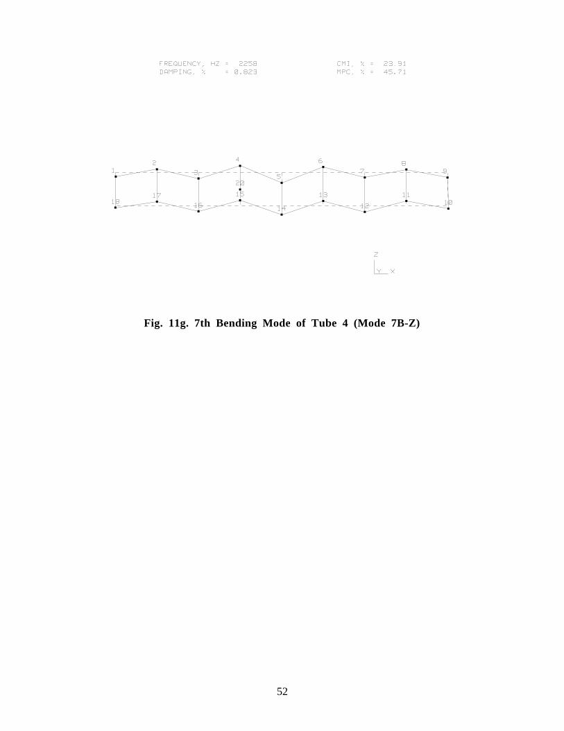
Figures 8 through 11 show the experimental mode shapes for tubes 1 through4, respectively. These wireframe plots show motions only at the 25

6

accelerometer positions used in the test. The measurements were mademostly in the Z direction (figure 3) and only motion in this direction isunderstandable. Additional sensors at other circumferential locations arenecessary to fully measure the modal characteristics.

Figure 12 shows the numerical correlation of the mode shapes for variouspairs of tubes using the Modal Assurance Criterion (MAC) (ref. 7). The size ofeach rectangle plotted in figure 12 is proportional to the corresponding MAC(0 - 100%). Pairs of modes with MAC values of at least 70 percent aredarkened for emphasis. This is an indication that the mode shapes are notaffected by the rubber layer.

Analysis Results

Analytical and experimental results were obtained for all 4 tubes.NASTRAN analysis determined 32 modes for tubes 1 and 3, and 134 modesfor tubes 2 and 4 that included the rigid body modes in the frequency range of0-2000 Hz. The increase in number of modes for tubes 2 and 4 is attributed tothe increase in flexibility of the tubes with the rubber layer.

The correlated mode shapes and corresponding analysis frequencies oftubes 1 and 3 are shown in figure 13a-13e. The modes consist of one Lovemode, three bending modes, and one breathing mode. The 3-D modes give abetter understanding of the complexity of the dynamic behavior of the tubes.Although a large number of modes were predicted by NASTRAN, no modescorrelated for tubes 2 and 4. Since there is no correlation between theexperimental data and analytical results for tubes 2 and 4 at the present time,only the correlation results for tube 1 and tube 3 will be discussed.

Correlation of Test and Analysis Results

In this work, the Modal Assurance Criteria (MAC) (ref. 7) was chosenfor correlation purposes. Each analysis mode shape is correlated with eachtest mode shape as follows:

MAC =ψ1

T j( )ψ 2 j( )j=1

n

∑2

ψ1T j( )ψ1 j( )(( ) ψ 2

T j( )ψ 2 j( )(( )j=1

n

∑j=1

n

∑(3)

where:ψ1= Analysis mode shapeψ 2 = Test mode shape

7

The MAC is a scalar value between zero and one that measuressimilarity of mode shapes. Values above 0.70 indicate a good match betweenthe compared modes.

Figures 14a and 14b show the numerical correlation of the mode shapesusing MAC for tubes 1 and 3, respectively.The size of each rectangle isproportional to the corresponding MAC (0-100%). Pairs of modes with MACvalues of at least 70 percent are darkened for emphasis. The analytical modeshapes which have a MAC value with the test results of at least 70% areplotted in figures 13a-13e. The test mode shapes for all the tubes are plotted infigures 8 - 12. Modes with high correlation include bending, breathing, andLove modes.

For tube 1, four modes matched between test and analysis as shown intable 4. The right side love mode had the best correlation. The measured andpredicted frequencies were 688 Hz and 523 Hz, respectively. The mode shapeis shown in figure 13a. The MAC value of 0.93 indicated that the modeshapes are practically identical. The first breathing mode had a MAC value of0.89 and measured and predicted frequencies of 808 Hz and 637 Hz,respectively. The mode shape is shown in figure 13b. The third result wasthe second breathing mode with measured and predicted frequencies of 845Hz and 788 Hz, respectively. The mode shape is shown in figure 13c. Thisresult had a correlation factor of 0.91. For the fourth mode, the measuredfrequency is 2195 Hz and the respective frequencies of the analysis mode is1926 Hz. The correlation factor is 0.87. This mode is the third bending shownin figure 13d.

Tube 3, had five modes that correlated between the analysis and testresults as shown in table 5. The first mode that correlated had a test frequencyof 724 Hz and analysis frequency of 523 Hz. The correlation factor or MACvalue was 0.94 and the mode was the R-love shown in figure 13a. The nextmode that correlated with a MAC value of 0.89 had test and predictedfrequencies of 854 Hz and 637 Hz, respectively. The mode type was the firstbreathing shown in figure 13b. The third mode was the second breathingmode shown in figure 13c. The MAC value of this correlation was 0.89 andthe test and predicted frequencies were 893 Hz and 788 Hz. The fourth modehad a test frequency of 1100 Hz and analysis frequency of 1142 Hz. The MACvalue was 0.76 and the mode was the third breathing mode shown in figure13d. The fifth test mode had a frequency of 2305 Hz and analysis frequency of1926 Hz. The MAC value was 0.82 shown in figure 13e.

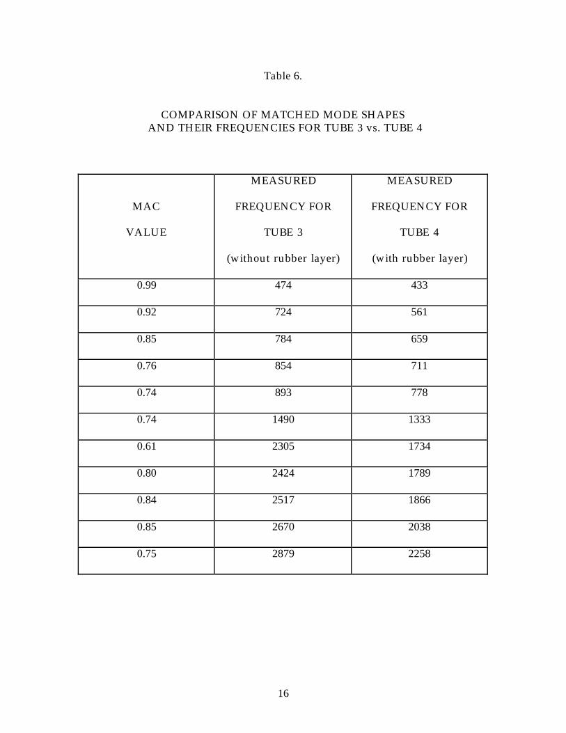
Test results were obtained and used to evaluate the effect of the rubberlayer. Table 6 shows the comparison of matched mode shapes and theirrespective frequencies for tube 3 without the rubber layer and tube 4 with therubber layer. There were 15 modes not including the rigid body modes thatmatched between these two tubes. The best correlation (with frequencies of474 Hz and 433 Hz, respectively) was mode 1. The MAC values ranged from0.99 to 0.61. The largest difference in frequencies occurred between modes no.

8

12 of tube 3 having a frequency of 2517 Hz and tube 4 having a frequency of1866 Hz. The frequencies for tube 4 were generally lower than for tube 3 onthe other hand damping values in tube 4 were higher than that in tube 3 dueto the presence of the rubber layer in table 6. The experimental frequenciesand damping values are summarized in table 3.

CONCLUDING REMARKS

This report described test and analysis results obtained for four graphiteepoxy missile tubes, two having an embedded layer of rubber. The rubberlayer significantly increased the damping of the structure which reducesvibration during operation. Measured modal damping factors (percent ofcritical damping) of the tubes without the rubber layer were approximately0.5%, increasing to approximately 2-3% for the tubes with the rubber layer.The embedded rubber layer also caused natural frequencies of the modes todecrease by approximately 10-20%.

Modal tests were performed using 25 accelerometer locations. Theseaccelerometer locations adequately measured the motion only in a singleplane passing through the centerline of the tube. Subsequent NASTRANanalytical predictions showed that additional measurement locations arenecessary to fully characterize the complex motion of the tubes in thefrequency range of interest (0-2000 Hz).

NASTRAN finite-element analysis predicted 26 elastic modes below 2000 forthe tubes without the rubber layer (tubes 1 and 3) and 128 elastic modes below2000 Hz for tubes with the rubber layer (tubes 2 and 4). The large increase inmodes is attributed to increased flexibility of the tubes having the rubberlayer. Based on the 25 available measurements, 4 of the NASTRAN modes oftube 1 and 5 of the NASTRAN modes of tube 3 correlated highly with the testresults. Unsatisfactory test-analysis correlation occurred for all modes of tubes2 and 4. It may be necessary to perform additional tests with moremeasurement locations in order to resolve the discepancies between test andanalysis due to the complex nature of the (predicted) mode shapes.

9

REFERENCES

1. Pappa, R. S., Elliott, K. B., Schenk, A, Consistent-Mode Indicator for theEigensystem Realization Algorithm, J. Guidance, Control, and Dynamics,Vol. 16, No. 5, Sept. 1993, pp. 852-858.

2. Pappa, R. S., Eigensystem Realization Algorithm User’s Guide forVAX/VMS Computers, Version 931216, NASA TM-109066, May 1994.

3. MSC/NASTRAN Handbook for Composite Analysis, The MacNeal-Schwendler Corporation, 1993.

4. I-DEAS Test Data Analysis User’s Guide, Structural Dynamics ResearchCorporation, 1990.

5. Tsai, S. W., Composite Design - 1985 , Think Composite, Dayton, OH, 1985.

6. Belvin R.D., Formulas For Natural Frequency and Mode Shape , KreigerPublishing Co., Malabar, FL, 1984.

7. Ewins, D. J., Modal Testing: Theory and Practice, John Wiley and SonsInc., New York, NY, 1984.

10

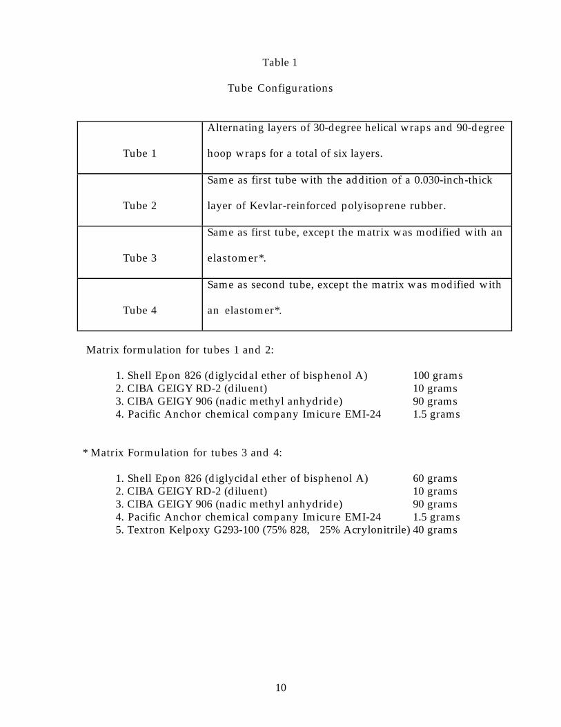
Table 1

Tube Configurations

Tube 1

Alternating layers of 30-degree helical wraps and 90-degree

hoop wraps for a total of six layers.

Tube 2

Same as first tube with the addition of a 0.030-inch-thick

layer of Kevlar-reinforced polyisoprene rubber.

Tube 3

Same as first tube, except the matrix was modified with an

elastomer*.

Tube 4

Same as second tube, except the matrix was modified with

an elastomer*.

Matrix formulation for tubes 1 and 2:

1. Shell Epon 826 (diglycidal ether of bisphenol A) 100 grams2. CIBA GEIGY RD-2 (diluent) 10 grams3. CIBA GEIGY 906 (nadic methyl anhydride) 90 grams4. Pacific Anchor chemical company Imicure EMI-24 1.5 grams

* Matrix Formulation for tubes 3 and 4:

1. Shell Epon 826 (diglycidal ether of bisphenol A) 60 grams2. CIBA GEIGY RD-2 (diluent) 10 grams3. CIBA GEIGY 906 (nadic methyl anhydride) 90 grams4. Pacific Anchor chemical company Imicure EMI-24 1.5 grams5. Textron Kelpoxy G293-100 (75% 828, 25% Acrylonitrile) 40 grams

11

Table 2.

MATERIAL PROPERTIES

Tube Configuration

Inside radius = 1.841 in

Thickness(without the layer of rubber) = 0.072 in

Tube length = 41 in

Tube weight(without the layer of rubber) = 2.416 lb

Composite structure properties Rubber properties

Ε1= 29.44x106 psi Ε

1=450 psi

Ε2= 1.624 x106 psi Ε

2= 450 psi

G12

=1.218 x106 psi G12

=200 psi

Gz1=1.218 x106 psi G

z1=200 psi

Gz2=1.218 x106 psi G

z2=200 psi

ν12

=0.32 ν12

=0.49

ρ=1.9913 x10--4lb/in3 ρ=0.89 x10--4 lb/in3

12

Table 3.Measured Frequencies and Damping of Tubes 1- 4

(a) TUBE 1

ModeNatural

Frequency,Hz

DampingFactor,

%CMI, % MPC, %

1B-Z 459 0.26 98 992B-Z 1158 1.51 9 173B-Z 2195 0.63 93 99

4B-Z 2298 0.57 89 97

5B-Z 2387 0.69 90 99

6B-Z 2542 0.78 91 96

7B-Z 2754 0.85 96 98

R-Love 688 0.55 94 99

L-Love 726 0.52 97 99

1BR 808 0.20 98 99

2BR 845 0.46 95 98

3BR 1045 2.53 8 254BR 1430 1.84 64 705BR 1964 1.60 89 99

6BR 2489 1.22 32 65

(b) TUBE 2

ModeNatural

Frequency,Hz

DampingFactor,

%CMI, % MPC, %

1B-Z 431 0.32 98 1002B-Z 1184 5.08 5 323B-Z 1606 3.02 49 884B-Z 1674 2.83 74 905B-Z 1801 2.77 60 866B-Z 1958 2.14 50 967B-Z 2229 1.99 17 78

R-Love 555 2.79 67 84L-Love 575 2.73 88 93

1BR 691 3.28 89 98

2BR 741 2.27 94 99

3BR 911 3.14 47 614BR 1377 2.65 72 865BR 1745 2.86 28 726BR 2434 1.73 80 94

13

(c) TUBE 3

ModeNatural

Frequency,Hz

DampingFactor,

%CMI, % MPC, %

1B-Z 474 0.26 98 992B-Z 1178 3.15 23 393B-Z 2305 0.29 70 924B-Z 2424 0.60 88 93

5B-Z 2517 0.63 90 96

6B-Z 2670 0.97 84 92

7B-Z 2879 0.79 96 99

R-Love 724 0.49 97 99

L-Love 784 1.02 79 801BR 854 0.18 97 98

2BR 893 0.69 83 86

3BR 1100 1.60 74 774BR 1490 2.51 35 385BR 2064 1.19 93 97

6BR 2600 1.40 63 78

(d) TUBE 4

ModeNatural

Frequency,Hz

DampingFactor,

%CMI, % MPC, %

1B-Z 433 0.32 99 1002B-Z 1061 1.77 16 203B-Z 1675 2.31 38 464B-Z 1734 2.39 72 945B-Z 1865 2.39 52 906B-Z 2037 1.86 85 97

7B-Z 2258 0.82 24 46R-Love 560 3.53 48 92L-Love 659 2.99 34 83

1BR 712 2.17 82 97

2BR 778 1.81 95 99

3BR 989 2.88 48 544BR 1332 2.06 71 785BR 1789 2.08 58 786BR 1969 2.11 73 96

14

Table 4.

COMPARISON OF MATCHED MODE SHAPES AND THEIR FREQUENCIES FOR TUBE 1.

MAC

VALUE

MEASURED

FREQUENCY

COMPUTED

FREQUENCY

MODE

TYPE

0.93 688 523

Right-side Love

Fig. 8h / Fig. 13a

0.89 808 637

1st Breathing

Fig. 8j / Fig. 13b

0.91 845 788

2nd Breathing

Fig. 8k / Fig. 13c

0.87 2195 1926

3rd Bending - Z

Fig. 8c / Fig. 13d

15

Table 5.

COMPARISON OF MATCHED MODE SHAPES AND THEIR FREQUENCIES FOR TUBE 3.

MAC

VALUE

MEASURED

FREQUENCY

COMPUTED

FREQUENCY

MODE

TYPE

0.94 724 523Right-side Love

Fig. 10h / Fig. 13a

0.89 854 6371st Breathing

Fig. 10j / Fig. 13b

0.89 893 7882nd Breathing

Fig. 10k / Fig. 13c

0.76 1100 11423rd Breathing

Fig. 10I / Fig. 13d

0.82 2305 19263rd Bending - Z

Fig. 10c / Fig. 13e

16

Table 6.

COMPARISON OF MATCHED MODE SHAPES AND THEIR FREQUENCIES FOR TUBE 3 vs. TUBE 4

MAC

VALUE

MEASURED

FREQUENCY FOR

TUBE 3

(without rubber layer)

MEASURED

FREQUENCY FOR

TUBE 4

(with rubber layer)

0.99 474 433

0.92 724 561

0.85 784 659

0.76 854 711

0.74 893 778

0.74 1490 1333

0.61 2305 1734

0.80 2424 1789

0.84 2517 1866

0.85 2670 2038

0.75 2879 2258

17

(a) Test Article

(All 4 tubes are similar in appearance)

41 in.

Composite layersincluding rubber

0.072-0.102 in

3.6 in Depending on layup

(b) Geometry

Figure 1. Graphite epoxy tubes

18

RUBBER

90

30

90

30

90

30

inside diameter

Outside surface

Inside surface

Rubber

+ / −

+ / −

+ / −

Angle with respectto tube axis

Figure 2. Composite layup

19

(a) Test Location Numbers

Location: 1 2 3 4 5 6 7 8 9 10 11 12 13 14 15 16 17 18 20

X xY xZ x x

(b) Excitation Positions (4)

Location: 1 2 3 4 5 6 7 8 9 10 11 12 13 14 15 16 17 18 20

X x x xY x x x xZ x x x x x x x x x x x x x x x x x x

(c) Accelerometer Positions (25)

Fig. 3. Test Set-Up

20

Fig. 4a. Driving-Point FRF for Tube 1 at Position 15Z

--------------------------------------------------------------------------------------

Fig. 4b. Driving-Point FRF for Tube 2 at Position 15Z

21

Fig. 4c. Driving-Point FRF for Tube 3 at Position 15Z

--------------------------------------------------------------------------------------

Fig. 4d. Driving-Point FRF for Tube 4 at Position 15Z

22

Figure 5. Finite Element Model

23

YX

Z

FINITE ELEMENT MODEL

ACCELEROMETERS

= TRIPLE AXIS ACCELEROMETERS

= SINGLE AXIS ACCELEROMETERS

Figure 6. Accelerometer locations and coordinate system.

24

Figure 7a. Transient Response for node 10374 in y-direction. First bending mode decay

Figure 7b. Location of the node 10374 on the Finite Element model

25

Fig. 8a. 1st Bending Mode of Tube 1 (Mode 1B-Z)

--------------------------------------------------------------------------------------

Fig. 8b. 2nd Bending Mode of Tube 1 (Mode 2B-Z)

26

Fig. 8c. 3rd Bending Mode of Tube 1 (Mode 3B-Z)

--------------------------------------------------------------------------------------

Fig. 8d. 4th Bending Mode of Tube 1 (Mode 4B-Z)

27

Fig. 8e. 5th Bending Mode of Tube 1 (Mode 5B-Z)

--------------------------------------------------------------------------------------

Fig. 8f. 6th Bending Mode of Tube 1 (Mode 6B-Z)

28

Fig. 8g. 7th Bending Mode of Tube 1 (Mode 7B-Z)

29

Fig. 8h. Rightside Love Mode of Tube 1 (Mode R-Love)

--------------------------------------------------------------------------------------

Fig. 8i. Leftside Love Mode of Tube 1 (Mode L-Love)

30

Fig. 8j. 1st Breathing Mode of Tube 1 (Mode 1BR)

--------------------------------------------------------------------------------------

Fig. 8k. 2nd Breathing Mode of Tube 1 (Mode 2BR)

31

Fig. 8l. 3rd Breathing Mode of Tube 1 (Mode 3BR)

--------------------------------------------------------------------------------------

Fig. 8m. 4th Breathing Mode of Tube 1 (Mode 4BR)

32

Fig. 8n. 5th Breathing Mode of Tube 1 (Mode 5BR)

--------------------------------------------------------------------------------------

Fig. 8o. 6th Breathing Mode of Tube 1 (Mode 6BR)

33


--------------------------------------------------------------------------------------


34


--------------------------------------------------------------------------------------


35


--------------------------------------------------------------------------------------


36


37


--------------------------------------------------------------------------------------


38


--------------------------------------------------------------------------------------


39


--------------------------------------------------------------------------------------


40


--------------------------------------------------------------------------------------


41


--------------------------------------------------------------------------------------


42


--------------------------------------------------------------------------------------


43


--------------------------------------------------------------------------------------


44


45


--------------------------------------------------------------------------------------


46


--------------------------------------------------------------------------------------


47


--------------------------------------------------------------------------------------


48


--------------------------------------------------------------------------------------


49


--------------------------------------------------------------------------------------


50


--------------------------------------------------------------------------------------


51


--------------------------------------------------------------------------------------


52


53


--------------------------------------------------------------------------------------


54


--------------------------------------------------------------------------------------


55


--------------------------------------------------------------------------------------


56


--------------------------------------------------------------------------------------


57

Fig. 12a. Correlation of Tube 1 and Tube 2 Mode Shapes

--------------------------------------------------------------------------------------

Fig. 12b. Correlation of Tube 1 and Tube 3 Mode Shapes

58

Fig. 12c. Correlation of Tube 1 and Tube 4 Mode Shapes--------------------------------------------------------------------------------------

Fig. 12d. Correlation of Tube 2 and Tube 3 Mode Shapes

59

Fig. 12e. Correlation of Tube 2 and Tube 4 Mode Shapes--------------------------------------------------------------------------------------

Fig. 12f. Correlation of Tube 3 and Tube 4 Mode Shapes

60

Figure 13a - Computed Right side Love Mode fortubes 1 and 3 (Frequency = 523 Hz)

61

Figure 13b - Computed 1st Breathing Mode fortubes 1 and 3 (Frequency = 637 Hz)

62

Figure 13c - Computed 2nd Breathing Mode for tubes 1 and 3 (Frequency = 788 Hz)

63

Figure 13d - Computed 3rd Breathing Mode for tubes 1 and 3 (Frequency = 1142 Hz)

64

Figure 13e- Computed 3rd Bending Mode for tube 3 (Frequency = 1926 Hz)

65

14a Test - Analysis Correlation for Tube 1

14b Test - Analysis Correlation for Tube 3

Figure 14. Modal Assurance Criterias for tube1 and 3

Finite-Element Vibration Analysis and Modal Testing of...

Documents

Transcript of Finite-Element Vibration Analysis and Modal Testing of...