Finite Element Transient Analysis - Civil · PDF fileFinite Element Transient Analysis V2.1...
67
Finite Element Transient Analysis version 2.1.00 Copyright 1996-2008 Dr. D.C. Rizos Contact Information Email [email protected] phone (803) 777-6166 User's Manual
Transcript of Finite Element Transient Analysis - Civil · PDF fileFinite Element Transient Analysis V2.1...

Finite Element Transient Analysis
version 2.1.00
Copyright 1996-2008
Dr. D.C. Rizos
Contact Information Email [email protected]
phone (803) 777-6166
User's Manual

Finite Element Transient Analysis V2.1 Dr. D.C. Rizos Copyright 1996-2008
7. Methodologies of Solution
Governing Equation The governing equations of motion of a multi-degree of freedom (MDOF) system can be cast in a matrix form as,
( ) ( ) ( ) ( )M C K f&& &u t u t u t t+ + = 7.1 where M, C, and K are the mass, damping and stiffness matrices of the dynamic system, u(t) represents the displacements of the nodal points of the system, f(t) are the nodal equivalent forces, and dots indicate differentiation with respect to time. The mass, damping and stiffness matrices are assembled from the respective element matrices as discussed in the Element Library section.
Support Conditions and External Loading The support conditions for both 2-D and 3-D dynamic systems pertain to restrains of the degrees of freedom of individual nodes or group of nodes of the finite element mesh. The external loading cases of the system are of the form of time histories of several types of excitations. Nodal forces and moments can be defined directly on the unrestrained nodes of the mesh. In the loading situation where known displacement and rotation time histories are prescribed, the corresponding degrees of freedom need to be restrained. To this end, program FETA automatically identifies the nodes subjected to forced motion and restrains the appropriate degrees of freedom. Ground motion in the form of known time histories of displacement, velocity and acceleration, is also accommodated.
Frequency Domain Solution For frequency domain analysis the solution is obtained in the form of a complex frequency response by letting the forcing function to be of the form
( )f t f eoi t= ω 7.2
The steady state response to this excitation has the same frequency as the exciting force and is expressed in terms of the complex frequency response, U, as,
u Uei t= ω 7.3
Substitution of equation 7.3 and its derivatives into equation 7.1 gives the governing equation adopted in FETA for frequency domain analysis, as

Finite Element Transient Analysis V2.1 Dr. D.C. Rizos Copyright 1996-2008
( )− + + =M C K U f2ω ωi o 7.4 The damping matrix C is evaluated on the basis of the hysteretic damping of the material. Equation 7.4 is solved for a series of frequencies ω for the complex frequency response U. Subsequently, the time history of the displacements can be obtained through a Fourier transformation of the complex response to the time domain. In the event that soil-structure models are considered, the far field is assumed to be a horizontally layered region. Each layer is a linearly elastic, isotropic medium. The far field extends to infinity in all horizontal directions, and its surface is free of tractions. At the base of the far field, two possibilities are available in FETA: rigid bedrock or a homogeneous, linearly elastic, isotropic half-space. The representation of the far field as a hyperelement is accomplished in the frequency domain by the finite element method. An expression of far-field motion in terms of semi-discrete wave modes (vertically discrete, horizontally continuous) is the basis of the formulation. Brief descriptions of the hyperelements implemented in FETA for two-dimensional as well as three-dimensional frequency domain computations are given in chapter Element Library.
Time Domain Solution For direct time domain analysis the solution the governing equation of motion 7.1 is obtained in the time marching scheme derived by the Newmark-β method. The mass, damping and stiffness matrices are assembled from the corresponding element matrices. The external excitation is in the form of time histories of nodal forces, or displacements. In the event that infinite soil regions are considered in the soil-structure model, the boundary of the finite domain is complemented by absorbing elements consisting of uniformly distributed dashpots, as defined in the Element Library section.
Newmark-β Method The direct numerical integration in time of second order differential equations of motion may be formulated as some type of finite difference scheme. To this end, program FETA implements the Newmark-β method for the computation of direct time domain solutions of the considered elastodynamic systems. This method is preferred because of its controlled stability characteristics. Furthermore, this method accomodates iterative schemes of the solution of nonlinear dynamic systems. The first step of any direct numerical integration method is the definition of a time knot sequence, tj. On the basis of this time knot sequence, Newmark presented equations for approximating the displacement and velocity at time tj+1 which for a multi degree of freedom system are as follows
( )[ ]( )[ ]
Δ
ΔΔ
Δ
t t t
tt
t
j j j
j j j j j
j j j j j
= −
= + + − +
= + − +
+
+ +
+ +
1
1
2
2 2 1
1 1 1 1
21
1
u u u u u
u u u u
& && &&
& & && &&
β β
β β
7.5

Finite Element Transient Analysis V2.1 Dr. D.C. Rizos Copyright 1996-2008 where β1, and β2 are the Newmark-β coefficients, and subscripts indicated the time step. Equation #.2 together with the dynamic Equation #.1 are used to determine the three unknowns && , & ,u u uj j j+ + +1 1 1. First the displacement at step j+1 is evaluated as,
( )( )
( )
( )
u M CK
C u u
u u
M u u u
j j j j
j j j
j j j
tt
xt
f t
t u tt
tt
+
−
+= + +⎛
⎝⎜
⎞
⎠⎟
−β− + −
⎧⎨⎪
⎩⎪
−β + + −⎛
⎝⎜
⎞
⎠⎟⎫⎬⎪
⎭⎪
+ + + −⎧⎨⎪
⎩⎪
⎫⎬⎪
⎭⎪
1 12
2 12
2
1 1
1
2
2
2
2
2 21
21
21
ββ
β
β
β
ΔΔ Δ
Δ
Δ ΔΔ
ΔΔ
& &&
& &&
& &&
7.6
Subsequently, the velocity and acceleration are computed by solving the system of Equations 7.5.
The parameter β1 introduces numerical (algorithmic) damping within the step Δtj. If β1 is taken to be equal to 0.5 then no numerical damping is considered. Values of β1 less than 0.5 produce negative damping. If β1 is taken greater than 0.5 then positive artificial damping is introduced. The parameter β2 controls the variation of acceleration within the time step. For example if β2 is taken equal to 0 then the acceleration is constant within the step. The method is unconditionally stable for values of the β coefficients satisfying the inequality β β2 1 0 5≥ ≥ . .
Solution of the System of Equations. The dynamic governing equations are solved in the time marching scheme introduced by the Newmark-β method. First a sequence of equally spaced time knots is defined on the time axis. Subsequently, the equations of motion can be written for step j and solved for step j+1 in terms of the field variables at step j and j+1 as,
Du fj j jb+ += +1 1 7.7 where
Finite Element Transient Analysis V2.1 Dr. D.C. Rizos Copyright 1996-2008
D M CK
= + +⎛
⎝⎜
⎞
⎠⎟β
β1
22
2Δ
Δt
t 7.8
f fj jt
+ +=−β
12
2
12Δ
7.9
( )( ) ( )
( )
b t t u tt
tt
j j j j j j
j j j
+ = − + − − + + −⎛
⎝⎜
⎞
⎠⎟
⎧⎨⎪
⎩⎪
⎫⎬⎪
⎭⎪
+ + + −⎧⎨⎪
⎩⎪
⎫⎬⎪
⎭⎪
1 1 1
2
2
2
2
12
1
21
C u u u u
M u u u
& && & &&
& &&
Δ Δ ΔΔ
ΔΔ
β β β
β
7.10
The system of equations 7.7 is solved for the unknown variables at step j+1. To this end, a real arithmetic frontal solver is developed on the basis of the work presented by Irons [1]. This algorithm is based on a Gauss elimination scheme. However, it is more involved than the standard band-matrix algorithms, but is more efficient especially in the case where higher order elements are considered. In addition, for the present time marching scheme, an efficient technique to accommodate multiple right hand sides is implemented. For linear applications the coefficient matrix, D, needs to be evaluated once and the system of equations 7.7 is solved for the different right hand sides defined by equations 7.9 and 7.10. For nonlinear elastic applications, the coefficient matrix D is time dependent and is evaluated at every time step, provided that the stress-strain relationships are defined.

Finite Element Transient Analysis V2.1 Dr. D.C. Rizos Copyright 1996-2008
8. ELEMENT LIBRARY This section describes the finite elements and their formulation as implemented in FETA. Tables 8.1-8.5 present a list of all available elements and their modeling features. Table 8.1 Structural Elements
Description Nodes Global Degrees of Freedom x y z θx θy θz
2D Axial force element for truss modeling 2 * * 3D Axial force element for truss modeling 2 * * * 2D Beam element for framed structures 2 * * * 3D Beam element for framed structures 2 * * * * * * 2D Linear Spring-Damper System 2 * * 3D Linear Spring-Damper System 2 * * * 2D Concentrated Mass 1 * * * 3D Concentrated Mass 1 * * * * * * 2D Concentrated Stiffness 1 * * * 3D Concentrated Stiffness 1 * * * * * * 3D Horizontal Plate 8 * * * 3D General Shell Element 8 * * * * * * Table 8.2 Soil/Solid Elements
Description Nodes Global Degrees of Freedom x y z θx θy θz
2D Constant Strain Triangle 3 * * 2D Linear Strain Triangle 6 * * 2D Constant Strain Quadrilateral 4 * * 2D Linear Strain Quadrilateral 8 * * 3D Linear Strain Tetrahedron 10 * * * 3D Linear Strain Pentahedron 15 * * * 3D Linear Strain Hexahedron 20 * * *

Finite Element Transient Analysis V2.1 Dr. D.C. Rizos Copyright 1996-2008 Table 8.3 Special Soil Elements
Description Nodes Global Degrees of Freedom x y z θx θy θz
2D Vertical Transmitting Boundaries varied * * 3D Vertical Cylindrical Transmitting
Bound. varied * * *
2D Absorbing Boundary 2 or 3 * * 3D Absorbing Boundary 6 or 8 * * * Table 8.4 Constraining Elements
Description Nodes Global Degrees of Freedom x y z θx θy θz
2D Rigid Link 3 * * 3D Rigid Link 3 * * * 2D Rigid Footing 3 * * * 3D Rigid Footing 3 * * * * * * 2D Frictional Interface 3 * * Table 8.5 Fluid Elements
Description Nodes Global Degrees of Freedom Q ∂Q/∂N x y z
2D Quadrilateral pressure element 4 * 2D Triangular pressure element 3 * 2D Fluid-Solid Interface element 3 * * * 2D Free surface fluid element 2
Finite Element Transient Analysis V2.1 Dr. D.C. Rizos Copyright 1996-2008
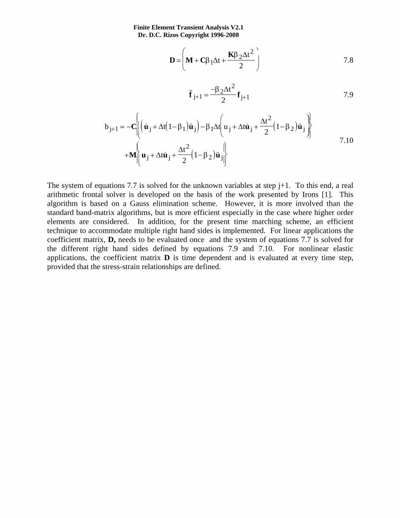
2-D Uniaxial Force Element The two dimensional uniaxial force element is a tension-compression element with two nodes. Each node has two translational degrees of freedom, in the global X and Y directions. The element can take only nodal forces and bending is not allowed. This element is used to model 2-D truss members.
Shape Functions The shape functions for the 2-D uniaxial element are
( ) ( )N112
1ξ ξ= − ( ) ( )N212
1ξ ξ= + 8.1
Stiffness Matrix The stiffness matrix of the 2D uniaxial tension-compression member is given in an explicit form as:
[ ]KEAL
l symlm ml lm llm m lm m
=− −− −
⎡
⎣
⎢⎢⎢⎢
⎤
⎦
⎥⎥⎥⎥
2
2
2 2
2 2
.
8.2
where l, and m are the directional cosines of the element defined as:
X
Y
ξ2
1
1
4
3
2
Finite Element Transient Analysis V2.1 Dr. D.C. Rizos Copyright 1996-2008
( ) ( )l
X X
X X Y Y=
−
− + −
2 1
2 12
2 12
( ) ( )
mY Y
X X Y Y=
−
− + −
2 1
2 12
2 12
8.3
Mass Matrix The mass matrix is evaluated according to the consistent formulation and is given in an explicit form as,
[ ]MAL
sym
=
⎡
⎣
⎢⎢⎢⎢
⎤
⎦
⎥⎥⎥⎥
ρ6
20 21 0 20 1 0 2
.
8.4
where ρ is the mass density
Damping Matrix For time domain analysis the damping matrix is evaluated according to the proportional damping formulation (Rayleigh damping) as a linear combination of the stiffness and mass matrices,
[ ] [ ] [ ]C a M b C= + 8.5 where a and b are user defined constants.
Finite Element Transient Analysis V2.1 Dr. D.C. Rizos Copyright 1996-2008
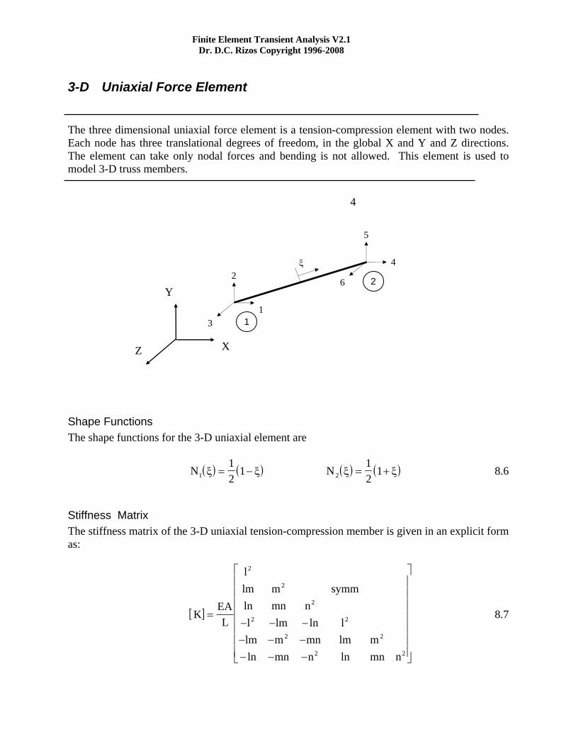
3-D Uniaxial Force Element The three dimensional uniaxial force element is a tension-compression element with two nodes. Each node has three translational degrees of freedom, in the global X and Y and Z directions. The element can take only nodal forces and bending is not allowed. This element is used to model 3-D truss members.
Shape Functions The shape functions for the 3-D uniaxial element are
( ) ( )N112
1ξ ξ= − ( ) ( )N212
1ξ ξ= + 8.6
Stiffness Matrix The stiffness matrix of the 3-D uniaxial tension-compression member is given in an explicit form as:
[ ]KEAL
llm m symm
mn nl lm llm m mn lm m
mn n mn n
=− − −− − −− − −
⎡
⎣
⎢⎢⎢⎢⎢⎢⎢
⎤
⎦
⎥⎥⎥⎥⎥⎥⎥
2
2
2
2 2
2 2
2 2
lnln
ln ln
8.7
X Z
Y
ξ
4
6
5
4
13
2 2
1

Finite Element Transient Analysis V2.1 Dr. D.C. Rizos Copyright 1996-2008 where l, m, and n are the directional cosines of the element defined as:
lX X
L=
−2 1 , mY Y
L=
−2 1 , nZ Z
L=
−2 1 8.8
( ) ( ) ( )L X X Y Y Z Z= − + − + −2 12
2 12
2 12
Mass Matrix The mass matrix is evaluated according to the consistent formulation and is given in an explicit form as,
[ ]MAL
=
⎡
⎣
⎢⎢⎢⎢⎢⎢⎢
⎤
⎦
⎥⎥⎥⎥⎥⎥⎥
ρ6
20 20 0 21 0 0 20 1 0 0 20 0 1 0 0 2
8.9
where ρ is the mass density
Damping Matrix For time domain analysis the damping matrix is evaluated according to the proportional damping formulation (Rayleigh damping) as a linear combination of the stiffness and mass matrices,
[ ] [ ] [ ]C a M b C= + 8.10 where a and b are user defined constants.

Finite Element Transient Analysis V2.1 Dr. D.C. Rizos Copyright 1996-2008
2-D Elastic Beam Element The two dimensional elastic beam element is a straight line element with two nodes. Each node has two translational, and one rotational degrees of freedom in the global coordinate system. The element takes either nodal forces or displacements. This element is used to model plane frame members.
Shape Functions The shape functions for the 2-D beam element are
( ) ( )N112
1ξ ξ= − ( )N23 22 3 1ξ ξ ξ= − + ( ) ( )N L3
3 22ξ ξ ξ ξ= − +
8.11
( ) ( )N 412
1ξ ξ= + ( )N 53 22 3ξ ξ ξ= − + ( ) ( )N L6
3 2ξ ξ ξ= −
and the displacement functions ux and uy are interpolated in terms of the nodal displacements ui as ( ) ( ) ( ) ( )u t N u t N u tx ( , )ξ ξ ξ= +1 1 4 4
8.12 ( ) ( ) ( ) ( ) ( ) ( ) ( ) ( ) ( )u t N u t N u t N u t N u ty ξ ξ ξ ξ ξ, = + + +2 2 3 3 5 5 6 6
X
Y
ξ
1
6
5
4
3
2
1
2

Finite Element Transient Analysis V2.1 Dr. D.C. Rizos Copyright 1996-2008 Stiffness Matrix The stiffness matrix of the 2D elastic beam member is given in an explicit form with respect to the element coordinate system as:
[ ]KEL
AI
Lsymm
IL
IA A
IL
IL
IL
IL
II
LI
= −
−
−
⎡
⎣
⎢⎢⎢⎢⎢⎢⎢⎢⎢⎢
⎤
⎦
⎥⎥⎥⎥⎥⎥⎥⎥⎥⎥
012
06
40 0
012 6
012
06
2 06
4
2
2 2
8.13
where A is the cross sectional area, and I is the moment of inertia.
Mass Matrix The mass matrix is evaluated according to the consistent formulation and is given in an explicit form with respect to the element coordinate system as,
[ ]MAL L L
LL L L L
=
− − −
⎡
⎣
⎢⎢⎢⎢⎢⎢⎢
⎤
⎦
⎥⎥⎥⎥⎥⎥⎥
ρ420
1400 1560 22 470 0 0 1400 54 13 0 1560 13 3 0 22 4
2
2 2
8.14
where ρ is the mass density.
Damping Matrix For time domain analysis the damping matrix is evaluated according to the proportional damping formulation (Rayleigh damping) as a linear combination of the stiffness and mass matrices,
[ ] [ ] [ ]C a M b C= + 8.15 where a and b are user defined constants.
3-D Elastic Beam Element

Finite Element Transient Analysis V2.1 Dr. D.C. Rizos Copyright 1996-2008 The three dimensional elastic beam element is a straight line element with two nodes. Each node has three translational and three rotational degrees of freedom, in the global coordinate system. The element takes either nodal forces or displacements. This element is used to model space frame members.
Shape Functions The shape functions for the 3-D beam element are
( ) ( )N1 0 5 1ξ ξ= −. , ( ) ( )N 2 0 5 1ξ ξ= +.
( ) ( )N321
21
23ξ
ξξ= − −
⎛⎝⎜
⎞⎠⎟ ( ) ( )N 4
212
12
3ξξ
ξ= + −⎛⎝⎜
⎞⎠⎟ 8.16
( ) ( )( )N520 5 1 1ξ ξ ξ= − −. ( ) ( )( )N 6
20 5 1 1ξ ξ ξ= + −. and the displacement functions ux, uy, uz, and θx are interpolated in terms of the nodal displacements ui as ( ) ( ) ( ) ( ) ( )u t u t N u t Nx ξ ξ ξ, = +1 1 7 2
( ) ( ) ( ) ( ) ( ) ( ) ( ) ( ) ( )( )u t u t N u t NL
u t N u t Ny ξ ξ ξ ξ ξ, = + + −2 3 8 4 6 5 12 68
( ) ( ) ( ) ( ) ( ) ( ) ( ) ( ) ( )( )u t u t N u t NL
u t N u t Nz ξ ξ ξ ξ ξ, = + − −3 3 9 4 5 5 11 68 8.17
( ) ( ) ( ) ( ) ( )θ ξ ξ ξx t u t N u t N, = +4 1 10 2
X Z
Y z
yx,ξ
1 12
11
10
9
8
7
6
5
4
3
2
1
2
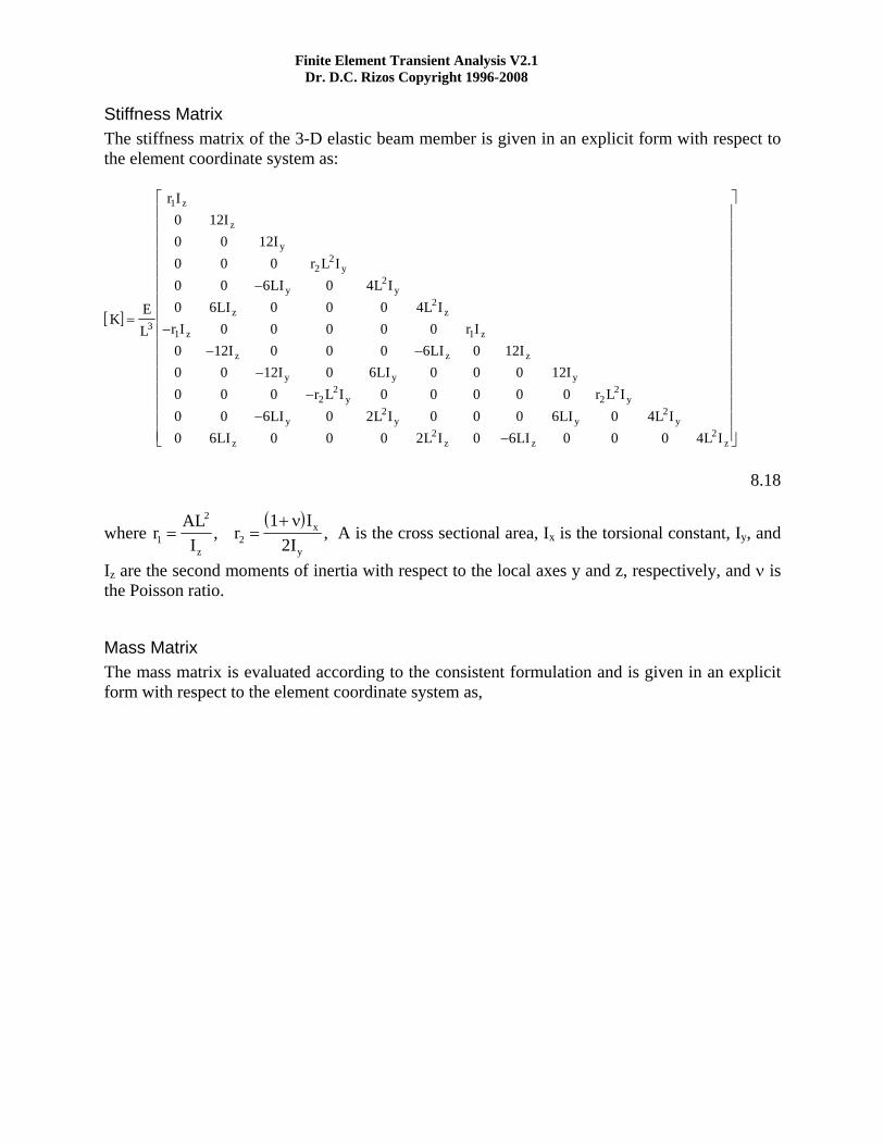
Finite Element Transient Analysis V2.1 Dr. D.C. Rizos Copyright 1996-2008 Stiffness Matrix The stiffness matrix of the 3-D elastic beam member is given in an explicit form with respect to the element coordinate system as:
[ ]KEL
r I
r L ILI L I
LI L Ir I r I
LILI
r L I r L ILI L I LI L I
LI L I LI L I
z
z
y
y
y y
z z
z z
z z z
y y y
y y
y y y y
z z z z
=
−
−− −
−−
−−
⎡
⎣
⎢⎢⎢⎢⎢⎢⎢⎢⎢⎢⎢⎢⎢⎢⎢⎢
⎤
3
1
22
2
2
1 1
22
22
2 2
2 2
0 12I0 0 12I0 0 00 0 6 0 40 6 0 0 0 4
0 0 0 0 00 12I 0 0 0 6 0 12I0 0 12I 0 6 0 0 0 12I0 0 0 0 0 0 0 00 0 6 0 2 0 0 0 6 0 40 6 0 0 0 2 0 6 0 0 0 4 ⎦
⎥⎥⎥⎥⎥⎥⎥⎥⎥⎥⎥⎥⎥⎥⎥⎥
8.18
where rALIz
1
2
= , ( )
rI
Ix
y2
12
=+ ν
, A is the cross sectional area, Ix is the torsional constant, Iy, and
Iz are the second moments of inertia with respect to the local axes y and z, respectively, and ν is the Poisson ratio.
Mass Matrix The mass matrix is evaluated according to the consistent formulation and is given in an explicit form with respect to the element coordinate system as,

Finite Element Transient Analysis V2.1 Dr. D.C. Rizos Copyright 1996-2008
[ ]MAL
rL L
L LL
LL
rL L L L L
L L L L
g
g
=
−
−
−
− −− − −
⎡
⎣
⎢⎢⎢⎢⎢⎢⎢⎢⎢⎢⎢⎢⎢⎢⎢⎢
⎤
⎦
⎥⎥⎥⎥⎥⎥⎥⎥⎥⎥⎥⎥⎥⎥⎥⎥
ρ420
1400 1560 0 1560 0 0 1400 0 22 0 40 22 0 0 0 470 0 0 0 13 0 1400 54 0 0 0 13 0 1560 0 54 13 0 0 0 0 1560 0 0 0 0 0 0 0 0 1400 0 13 3 3 0 0 0 22 0 40 13 0 0 0 3 0 22 0 0 0 4
2
2
2
2
2 2 2
2 2
8.19
where ρ is the mass density, and rg=J/A is the radius of gyration.
Damping Matrix For time domain analysis the damping matrix is evaluated according to the proportional damping formulation (Rayleigh damping) as a linear combination of the stiffness and mass matrices,
[ ] [ ] [ ]C a M b C= + 8.20 where a and b are user defined constants.

Finite Element Transient Analysis V2.1 Dr. D.C. Rizos Copyright 1996-2008
2-D Spring-Damper Element The two dimensional spring damper element is a tension-compression element with two nodes. Each node has two translational degrees of freedom, in the global X and Y directions. The element consists of a spring and a damper of known elastic properties. It can take only nodal forces and bending is not allowed. This element is used to model 2-D elastic links.
Stiffness Matrix The stiffness matrix of the 2D spring-damper element with respect to the global coordinate system is given in an explicit form as:
[ ]K k
l symlm ml lm llm m lm m
=− −− −
⎡
⎣
⎢⎢⎢⎢
⎤
⎦
⎥⎥⎥⎥
2
2
2 2
2 2
.
8.21
where k is the stiffness of the spring, and l, and m are the directional cosines of the element defined as:
( ) ( )l
X X
X X Y Y=
−
− + −
2 1
2 12
2 12
( ) ( )
mY Y
X X Y Y=
−
− + −
2 1
2 12
2 12
8.22
x
k
c
1
X
Y
1
2
2
3
4

Finite Element Transient Analysis V2.1 Dr. D.C. Rizos Copyright 1996-2008 Damping Matrix For time domain analysis the damping matrix is similar to the stiffness matrix, i.e.,
[ ]C c
l symlm ml lm llm m lm m
=− −− −
⎡
⎣
⎢⎢⎢⎢
⎤
⎦
⎥⎥⎥⎥
2
2
2 2
2 2
.
8.23
where c is the damping constant.

Finite Element Transient Analysis V2.1 Dr. D.C. Rizos Copyright 1996-2008
3-D Spring-Damper Element The three dimensional spring-damper element is a tension-compression element with two nodes. Each node has three translational degrees of freedom, in the global X, Y, and Z directions. The element consists of a spring and a damper of known elastic properties. It can take only nodal forces and bending is not allowed. This element is used to model 3-D elastic links.
Stiffness Matrix The stiffness matrix of the 3-D spring-damper element with respect to the global coordinate system is given in an explicit form as:
[ ]K k
llm m sym
mn nl lm llm m mn lm m
mn n mn n
=− − −− −− − −
⎡
⎣
⎢⎢⎢⎢⎢⎢⎢
⎤
⎦
⎥⎥⎥⎥⎥⎥⎥
2
2
2
2 2
2 2
2 2
.ln
ln
ln ln
8.24
where k is the spring stiffness, and l, m, and n are the directional cosines of the element defined as:
( ) ( )l
X X
X X Y Y=
−
− + −
2 1
2 12
2 12
x
k
c
1
X
Y
1
2
2
3
5
Z
6
4

Finite Element Transient Analysis V2.1 Dr. D.C. Rizos Copyright 1996-2008
( ) ( )m
Y Y
X X Y Y=
−
− + −
2 1
2 12
2 12
8.25
( ) ( )
nZ Z
X X Y Y=
−
− + −
2 1
2 12
2 12
Damping Matrix For time domain analysis the damping matrix is similar to the stiffness matrix, i.e.,
[ ]C c
llm m sym
mn nl lm llm m mn lm m
mn n mn n
=− − −− −− − −
⎡
⎣
⎢⎢⎢⎢⎢⎢⎢
⎤
⎦
⎥⎥⎥⎥⎥⎥⎥
2
2
2
2 2
2 2
2 2
.ln
ln
ln ln
8.26
where c is the damping constant.

Finite Element Transient Analysis V2.1 Dr. D.C. Rizos Copyright 1996-2008
2-D Concentrated Mass The two dimensional concentrated mass is a point element which has two translational and one rotational degrees of freedom, in the global coordinate system. The element consists of a lumped mass which presents inertia forces and moments. This element is used to add the influence of concentrated masses to the dynamic system.
Mass Matrix The mass matrix of the 2-D concentrated mass element with respect to the global coordinate system is a diagonal matrix given in an explicit form as:
[ ]Mm
mI
x
y=
⎡
⎣
⎢⎢⎢
⎤
⎦
⎥⎥⎥
0
8.27
where mx, and my are the masses contributing to the inertia forces in the X and Y direction, and Io is the mass moment of inertia associated to the moment.
X
Y
2
31
Θ

Finite Element Transient Analysis V2.1 Dr. D.C. Rizos Copyright 1996-2008
3-D Concentrated Mass The three dimensional concentrated mass is a point element which has three translational and three rotational degrees of freedom, in the global coordinate system. The element consists of a lumped mass which presents inertia forces and moments. This element is used to add the influence of concentrated masses to the 3-D dynamic system.
Mass Matrix The mass matrix of the 3-D concentrated mass element with respect to the global coordinate system is a diagonal matrix given in an explicit form as:
[ ]M
mm
mI
II
x
y
z
ox
oy
oz
=
⎡
⎣
⎢⎢⎢⎢⎢⎢⎢
⎤
⎦
⎥⎥⎥⎥⎥⎥⎥
8.28
where mx, my, and mz are the masses contributing to the inertia forces in the X, Y, and Z direction, respectively, and Iox, Ioy, Ioz, are the mass moments of inertia in the X, Y, and Z directions, respectively.
X
Y2
3
1
Z
4
5
6

Finite Element Transient Analysis V2.1 Dr. D.C. Rizos Copyright 1996-2008
2-D Elastic Stiffener The two dimensional elastic stiffener is a point element which has two translational and one rotational degrees of freedom, in the global coordinate system. The element consists of a stiffener which presents elastic forces and moments. This element is used to add the influence of stiffeners to the dynamic system.
Stiffness Matrix The stiffness matrix of the 2-D stiffener with respect to the global coordinate system is a diagonal matrix given in an explicit form as:
[ ]Kk
kk
x
y=
⎡
⎣
⎢⎢⎢
⎤
⎦
⎥⎥⎥θ
8.29
where kx, and ky are the stiffness coefficients contributing to the elastic forces in the X and Y direction, and kθ is the stiffness coefficient associated to the elastic moment.
X
Y
2
3 1
Θ
Finite Element Transient Analysis V2.1 Dr. D.C. Rizos Copyright 1996-2008
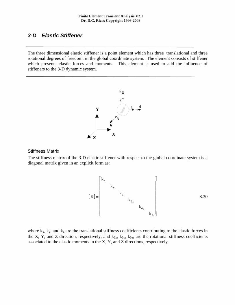
3-D Elastic Stiffener The three dimensional elastic stiffener is a point element which has three translational and three rotational degrees of freedom, in the global coordinate system. The element consists of stiffener which presents elastic forces and moments. This element is used to add the influence of stiffeners to the 3-D dynamic system.
Stiffness Matrix The stiffness matrix of the 3-D elastic stiffener with respect to the global coordinate system is a diagonal matrix given in an explicit form as:
[ ]K
kk
kk
kk
x
y
z
x
y
z
=
⎡
⎣
⎢⎢⎢⎢⎢⎢⎢
⎤
⎦
⎥⎥⎥⎥⎥⎥⎥
θ
θ
θ
8.30
where kx, ky, and kz are the translational stiffness coefficients contributing to the elastic forces in the X, Y, and Z direction, respectively, and kθx, kθy, kθz, are the rotational stiffness coefficients associated to the elastic moments in the X, Y, and Z directions, respectively.
X
Y
2
3
1
Z
4
5
6

Finite Element Transient Analysis V2.1 Dr. D.C. Rizos Copyright 1996-2008
3-D Horizontal Plate - Bending Only The element is of rectangular shape defined by eight geometric nodes and is parallel to the X-Y horizontal plane. Each node has one translational degree of freedom in the vertical Z direction, and two rotational degrees of freedom in the plane of the plate. It can take only vertical forces or bending moments.
Shape Functions The shape functions of the 8-node plate element are
( )( )( )
( )( )
( )( )
N i
N i
N i
i
i
i
= + + − + + =
= − + =
= + − =
14
1 1 1 1 2 3 4
12
1 1 5 7
12
1 1 6 8
0 0 0 0
20
02
ξ η ξ η
ξ η
ξ η
, , ,
,
,
8.31
Stiffness Matrix The element stiffness matrix is given as
X
Y
Z
ζ
ξ
η
1
2
3
4
56
78
w
θθ
xy
h
ξ
η

Finite Element Transient Analysis V2.1 Dr. D.C. Rizos Copyright 1996-2008
[ ] [ ] [ ][ ] [ ] [ ][ ]K B E Bh
B E B dAAT
A BT
BA
= +⎛
⎝⎜
⎞
⎠⎟∫∫ 2
6
2
8.32
where : [E] is the stress-strain matrix
[ ] ( )( )( )
( )
EE
sym
=+ −
−−
−
−
−
⎡
⎣
⎢⎢⎢⎢⎢⎢⎢⎢
⎤
⎦
⎥⎥⎥⎥⎥⎥⎥⎥
1 1 2
11
1 22
1 22 12
1 22 12
ν ν
νν ν
ν
ν
ν
.
.
.
8.33
the form factor (1.2) appearing in the last two terms of the stress-strain matrix accounts for the fact that the transverse shearing stresses produce too little strain energy [2]. [BA], and [BB] are matrices containing the shape functions and the associated derivatives, and consist of the sub-matrices
[ ] [ ]Bb Na N
B
aba bAi
i i
i i
Bi
i
i
i i=−
⎡
⎣
⎢⎢⎢⎢⎢⎢
⎤
⎦
⎥⎥⎥⎥⎥⎥
=
−−
⎡
⎣
⎢⎢⎢⎢⎢⎢
⎤
⎦
⎥⎥⎥⎥⎥⎥
0 0 00 0 00 0 0
00
0 00 000 0 00 0 0
8.34
with ai, and bi defined as
ab
NN
i
i
x x
y y
i x
i y
⎧⎨⎩
⎫⎬⎭
=⎡
⎣⎢
⎤
⎦⎥⎧⎨⎩
⎫⎬⎭
ξ ηξ η
, ,
, ,
,
, 8.35
The integral indicated in equation 8.32 is evaluated numerically using a standard Gaussian quadrature with the following points and weights:
ξ η weight 0-.774596669241483 -0.774596669241483 25/81

Finite Element Transient Analysis V2.1 Dr. D.C. Rizos Copyright 1996-2008
-0.774596669241483 0.0 40/81 -0.774596669241483 0.774596669241483 25/81
0.0 -0.774596669241483 40/81 0.0 0.0 64/81 0.0 0.774596669241483 40/81
0.774596669241483 -0.774596669241483 25/81 0.774596669241483 0.0 40/81 0.774596669241483 0.774596669241483 25/81
Mass Matrix The element mass matrix is evaluated from the integral
[ ] [ ] [ ] [ ] [ ]M N Nh
N N dAAT
A BT
BA
= +⎛
⎝⎜
⎞
⎠⎟∫∫ρ 2
6
2
8.36
with [NA], and [NB] being the following shape function matrices,
[ ] [ ]N N N NAi i Bi i=
⎡
⎣
⎢⎢⎢
⎤
⎦
⎥⎥⎥
= −
⎡
⎣
⎢⎢⎢
⎤
⎦
⎥⎥⎥
0 0 00 0 01 0 0
0 0 10 1 00 0 0
8.37
The integral indicated in equation 8.36 is evaluated numerically using a standard Gaussian quadrature with the points and weights shown in the Stiffness Matrix section.
Damping Matrix For time domain analysis the damping matrix is evaluated according to the proportional damping formulation (Rayleigh damping) as a linear combination of the stiffness and mass matrices,
[ ] [ ] [ ]C a M b C= + 8.38 where a and b are user defined constants.

Finite Element Transient Analysis V2.1 Dr. D.C. Rizos Copyright 1996-2008
3-D General Shell The element is of rectangular shape defined by eight geometric nodes and is arbitrarily oriented in the 3-D space. Each node has three translational degrees of freedom in the global coordinate system, and two rotational degrees of freedom in the plane tangent on the node under consideration.
Shape Functions The shape functions of the 8-node general shell element are
( )( )( )
( )( )
( )( )
N i
N i
N i
i
i
i
= + + − + + =
= − + =
= + − =
14
1 1 1 1 2 3 4
12
1 1 5 7
12
1 1 6 8
0 0 0 0
20
02
ξ η ξ η
ξ η
ξ η
, , ,
,
,
8.39
where ξ ξξo i= and η ηηo i=
X Y
Z
ξ
η
ζ
η
ξ
1
2
3
45
6
7
8
h

Finite Element Transient Analysis V2.1 Dr. D.C. Rizos Copyright 1996-2008
Stiffness Matrix The element stiffness matrix is given as
[ ] [ ] [ ][ ] [ ] [ ][ ]K B E B B E B dAAT
A BT
BA
= +⎛⎝⎜
⎞⎠⎟∫∫ 2
23
8.40
where : [E] is the stress-strain matrix
[ ] ( )( )( )
( )
EE
sym
=+ −
−−
−
−
−
⎡
⎣
⎢⎢⎢⎢⎢⎢⎢⎢
⎤
⎦
⎥⎥⎥⎥⎥⎥⎥⎥
1 1 2
11
1 22
1 22 12
1 22 12
ν ν
νν ν
ν
ν
ν
.
.
.
8.42
the form factor (1.2) appearing in the last two terms of the stress-strain matrix accounts for the fact that the transverse shearing stresses produce too little strain energy [2]. [BA], and [BB] are matrices containing the shape functions and the associated derivatives,
[ ] [ ]
[ ] [ ]
B T
a d l d lb e m e m
c g n g nb a e l d m e l d m
c b g m e n g m e nc a d n g l d n g l
Bh
T
a l a lb m b
Ai
i i i i i
i i i i i
i i i i i
i i i i i i i i i i
i i i i i i i i i i
i i i i i i i i i i
Bi
i i i i
i i
=
−−−
− − +− − +− − +
⎡
⎣
⎢⎢⎢⎢⎢⎢⎢
⎤
⎦
⎥⎥⎥⎥⎥⎥⎥
=
−−
0 00 00 0
00
0
2
0 0 00 0 0
2 1
2 1
2 1
2 2 1 1
2 2 1 1
2 2 1 1
2 1
2 i i
i i i i
i i i i i i i i
i i i i i i i i
i i i i i i i i
mc n c n
b l a m b l a mc m b n c m b na n c l a n c l
1
2 1
2 2 1 1
2 2 1 1
2 2 1 1
0 0 00 0 00 0 00 0 0
−− − +− − +− − +
⎡
⎣
⎢⎢⎢⎢⎢⎢⎢
⎤
⎦
⎥⎥⎥⎥⎥⎥⎥
8.43
The parameters ai, through gi are defined as

Finite Element Transient Analysis V2.1 Dr. D.C. Rizos Copyright 1996-2008
abcdeg
NNNNN
i
i
i
i
i
i
x x
y y
z z
x
y
z
i
i
i
i
i
⎧
⎨
⎪⎪⎪
⎩
⎪⎪⎪
⎫
⎬
⎪⎪⎪
⎭
⎪⎪⎪
=
⎡
⎣
⎢⎢⎢⎢⎢⎢⎢
⎤
⎦
⎥⎥⎥⎥⎥⎥⎥
⎧
⎨
⎪⎪⎪
⎩
⎪⎪⎪
⎫
⎬
⎪⎪⎪
⎭
⎪⎪⎪
ξ ηξ ηξ η
ζζ
ζ
ξ
η
, ,
, ,
, ,
,
,
,
,
,
0 0 00 0 00 0 0
0 0 0 00 0 0 00 0 0 0
8.44
Matrix [T] is the transformation matrix containing the directional cosines of the normal and tangential vectors at the integration point, and lji, mji, nji, j=1,2 represent the directional cosines of the two tangential vectors at node i. The integral indicated in equation 8.40 is evaluated numerically using a standard Gaussian quadrature with the points and weights listed in the element 3-D Horizontal Plate - Bending Only
Mass Matrix The element mass matrix is evaluated from the integral
[ ] [ ] [ ] [ ] [ ]M N N N N dAAT
A BT
BA
= +⎛⎝⎜
⎞⎠⎟∫∫ρ 2
23
8.45
with [NA], and [NB] being the following shape function matrices,
[ ] [ ]N N Nl l
m mn n
hNAi i Bi
i i
i i
i i
i=
⎡
⎣
⎢⎢⎢
⎤
⎦
⎥⎥⎥
=−
−−
⎡
⎣
⎢⎢⎢
⎤
⎦
⎥⎥⎥
1 0 0 0 00 1 0 0 00 0 1 0 0
0 0 00 0 00 0 0
2
2 1
2 1
2 1
8.46
The integral indicated in equation 8.45 is evaluated numerically using a standard Gaussian quadrature with the points and weights listed in the element 3-D Horizontal Plate - Bending Only
Damping Matrix For time domain analysis the damping matrix is evaluated according to the proportional damping formulation (Rayleigh damping) as a linear combination of the stiffness and mass matrices,
[ ] [ ] [ ]C a M b C= + 8.47 where a and b are user defined constants.
2-D Constant Strain Triangle

Finite Element Transient Analysis V2.1 Dr. D.C. Rizos Copyright 1996-2008 This is a triangular element defined by three geometric nodes. Each node has two translational degrees of freedom in the global coordinate system. It is used to model two dimensional plane strain solids and soils.
Shape Functions The shape functions of the 3-node constant strain triangle are
N L ii i= = 1 3,2, 8.48
where Li are the area coordinates.
Stiffness Matrix The element stiffness matrix is given as
[ ] [ ] [ ][ ]K B D B dAT
A
= ∫ 8.49
where [D] is the elasticity matrix for a plane strain isotropic material expressed as,
[ ] ( )( )( )
( )( )
DE
=−
+ −
−
−−
−
⎡
⎣
⎢⎢⎢⎢⎢⎢
⎤
⎦
⎥⎥⎥⎥⎥⎥
11 1 2
11
0
11 0
0 01 2
2 1
νν ν
νν
νν
νν
8.50
and [B] consists of the sub-matrices [B]i, I=1,2,3, defined as
Y1
2
3
4
5
6
1
2
3
L1
L2
L3

Finite Element Transient Analysis V2.1 Dr. D.C. Rizos Copyright 1996-2008
[ ]B
Nx
Ny
Ny
Nx
i
i
i
i i
=
⎡
⎣
⎢⎢⎢⎢⎢⎢
⎤
⎦
⎥⎥⎥⎥⎥⎥
∂∂
∂∂
∂∂
∂∂
0
0 8.51
The integral indicated in equation 8.49 is evaluated numerically using a standard Gaussian quadrature with one integration point at L1=L2=L3=1/3 and corresponding weight w=1.0
Mass Matrix The element mass matrix is evaluated on the basis of the consistent formulation as
[ ] [ ] [ ]M N N dAT
A
= ∫ρ 8.52
where ρ is the mass density of the elastic medium, and the integral is evaluated numerically, similarly to the stiffness matrix.
Damping Matrix For time domain analysis the damping matrix is evaluated according to the proportional damping formulation (Rayleigh damping) as a linear combination of the stiffness and mass matrices,
[ ] [ ] [ ]C a M b C= + 8.53 where a and b are user defined constants.

Finite Element Transient Analysis V2.1 Dr. D.C. Rizos Copyright 1996-2008
2-D Linear Strain Triangle This is a triangular element defined by six geometric nodes. Each node has two translational degrees of freedom in the global coordinate system. It is used to model two dimensional plane strain solids and soils.
Shape Functions The shape functions of the 6-node linear strain triangle are
( )N L L iN L L i p i q i
i i i
i p q
= − =
= = = − = −
2 1 1 34 4 5 3 2
,2,, ,6, ,
8.54
where Li are the area coordinates.
Stiffness Matrix The element stiffness matrix is given as
[ ] [ ] [ ][ ]K B D B dAT
A
= ∫ 8.55
where [D] is the elasticity matrix for a plane strain isotropic material defined in equation 8.50, and [B] consists of the sub-matrices [B]i, i=1,2,...,6 defined in equation 8.51. The integral indicated in equation 8.55 is evaluated numerically using a standard Gaussian quadrature with the integration points and weights defined in Table 8.6.
Y1
2
34
5
6
1
L1
L2
L3
7
8
4 2
5
3
6
9
1011
12

Finite Element Transient Analysis V2.1 Dr. D.C. Rizos Copyright 1996-2008 Table 8.6 Integration Points and Weights
L1 L2 L3 W 0.5 0.5 0.0 1/3 0.0 0.5 0.5 1/3 0.5 0.0 0.5 1/3
Mass Matrix The element mass matrix is evaluated on the basis of the consistent formulation as
[ ] [ ] [ ]M N N dAT
A
= ∫ρ 8.56
where ρ is the mass density of the elastic medium, and the integral is evaluated numerically using a standard Gaussian quadrature with the integration points and weights defined in Table 8.6.
Damping Matrix For time domain analysis the damping matrix is evaluated according to the proportional damping formulation (Rayleigh damping) as a linear combination of the stiffness and mass matrices,
[ ] [ ] [ ]C a M b C= + 8.57 where a and b are user defined constants.

Finite Element Transient Analysis V2.1 Dr. D.C. Rizos Copyright 1996-2008
2-D Constant Strain Quadrilateral This is a triangular element defined by four geometric nodes. Each node has two translational degrees of freedom in the global coordinate system. It is used to model two dimensional plane strain solids and soils.
Shape Functions The shape functions of the 4-node constant strain triangle are
( )( ) ( )( )
( )( ) ( )( )
N N
N N
1 2
3 4
14
1 114
1 1
14
1 114
1 1
= − − = + −
= + + = − +
ξ η ξ η
ξ η ξ η 8.58
Stiffness Matrix The element stiffness matrix is given as
[ ] [ ] [ ][ ]K B D B dAT
A
= ∫ 8.59
Y
X
1
2
1
7
8
4
34
2
5
6
3
ξ
η
ξ
η
1 2
34
(−1,−1)
(1,1)

Finite Element Transient Analysis V2.1 Dr. D.C. Rizos Copyright 1996-2008 where [D] is the elasticity matrix for a plane strain isotropic material defined in equation 8.50, and [B] consists of the sub-matrices [B]i, i=1,2,3,4 defined in equation 8.51. The integral indicated in equation 8.59 is evaluated numerically using a standard Gaussian quadrature with the integration points and weights defined in Table 8.7. Table 8.7 Integration Points and Weights
ξ η w
-0.577350269189626 -0.577350269189626 1.0
0.577350269189626 -0.577350269189626 1.0
0.577350269189626 0.577350269189626 1.0
-0.577350269189626 0.577350269189626 1.0
Mass Matrix The element mass matrix is evaluated on the basis of the consistent formulation as
[ ] [ ] [ ]M N N dAT
A
= ∫ρ 8.60
where ρ is the mass density of the elastic medium, and the integral is evaluated numerically using a standard Gaussian quadrature with the integration points and weights defined in Table 8.7.
Damping Matrix For time domain analysis the damping matrix is evaluated according to the proportional damping formulation (Rayleigh damping) as a linear combination of the stiffness and mass matrices,
[ ] [ ] [ ]C a M b C= + 8.61 where a and b are user defined constants.

Finite Element Transient Analysis V2.1 Dr. D.C. Rizos Copyright 1996-2008
2-D Linear Strain Quadrilateral This is a triangular element defined by eight geometric nodes. Each node has two translational degrees of freedom in the global coordinate system. It is used to model two dimensional plane strain solids and soils.
Shape Functions The shape functions of the 4-node constant strain triangle are
( )( )( ) ( )( )( )
( )( )( ) ( )( )( )
( )( ) ( )( )
( )( ) ( )( )
N N
N N
N N
N N
1 2
3 4
52
62
72
62
14
1 1 114
1 1 1
14
1 1 114
1 1 1
12
1 112
1 1
12
1 112
1 1
= − − − − − = + − − + −
= + + − + + = − + − − +
= − − = + −
= + − = − −
ξ η ξ η ξ η ξ η
ξ η ξ η ξ η ξ η
η ξ ξ η
η ξ ξ η
8.62
Y
X
1
2
1
7
8
4
34
2
5
6
3
η
1 2
34
(−1,−1)
(1,1)
910
5
11
12
6
13
14
7
15
16
8
6
7
8
5

Finite Element Transient Analysis V2.1 Dr. D.C. Rizos Copyright 1996-2008 Stiffness Matrix The element stiffness matrix is given as
[ ] [ ] [ ][ ]K B D B dAT
A
= ∫ 8.63
where [D] is the elasticity matrix for a plane strain isotropic material defined in equation 8.50, and [B] consists of the sub-matrices [B]i, i=1,2,...,8 defined in equation 8.51. The integral indicated in equation 8.62 is evaluated numerically using a standard Gaussian quadrature with the integration points and weights defined in Table 8.8 Table 8.8 Integration Points and Weights
ξ η w
-0.774596669241483 -0.774596669241483 1/3.24
0.0 -0.774596669241483 1/2.025
0.774596669241483 -0.774596669241483 1/3.24
-0.774596669241483 0.0 1/2.025
0.0 0.0 1/1.265625
0.774596669241483 0.0 1/2.025
-0.774596669241483 0.774596669241483 1/3.24
0.0 0.774596669241483 1/2.025
0.774596669241483 0.774596669241483 1/3.24
Mass Matrix The element mass matrix is evaluated on the basis of the consistent formulation as
[ ] [ ] [ ]M N N dAT
A
= ∫ρ 8.64
where ρ is the mass density of the elastic medium, and the integral is evaluated numerically.
Finite Element Transient Analysis V2.1 Dr. D.C. Rizos Copyright 1996-2008
Damping Matrix For time domain analysis the damping matrix is evaluated according to the proportional damping formulation (Rayleigh damping) as a linear combination of the stiffness and mass matrices,
[ ] [ ] [ ]C a M b C= + 8.65 where a and b are user defined constants.

Finite Element Transient Analysis V2.1 Dr. D.C. Rizos Copyright 1996-2008
3-D 10 Node Tetrahedron This is a solid element defined by ten geometric nodes. Each node has three translational degrees of freedom in the global coordinate system. It is used to model three dimensional solids and soils.
Shape Functions The shape functions of the 3-node constant strain triangle are
( )N L L iN L L N L L N L LN L L N L L N L L
i i i= − =
= = == = =
2 1 1 3 44 4 44 4 4
5 1 2 6 2 3 7 3 1
8 1 4 9 2 4 10 3 4
,2, , 8.66
where Li are the volume coordinates
Stiffness Matrix The element stiffness matrix is given as
[ ] [ ] [ ][ ]K B D B dAT
A
= ∫ 8.67
where [D] is the elasticity matrix for an isotropic material expressed as,
3
2
4
6
810
1
9
7
Z
XY
L2
1
2
3
4
5 6
78
910
1314
15
5
Finite Element Transient Analysis V2.1 Dr. D.C. Rizos Copyright 1996-2008
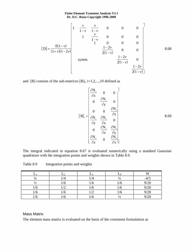
[ ]( )
( )( ) ( )
( )
( )
DE
symm
=−
+ −
− −
−
−−
−−
−−
⎡
⎣
⎢⎢⎢⎢⎢⎢⎢⎢⎢⎢⎢
⎤
⎦
⎥⎥⎥⎥⎥⎥⎥⎥⎥⎥⎥
11 1 2
11 1
0 0 0
11
0 0 01 0 0 0
1 22 1
0 0
1 22 1
0
1 22 1
νν ν
νν
νν
νν
νν
νν
νν
.
8.68
and [B] consists of the sub-matrices [B]i, i=1,2,...,10 defined as
[ ]B
Nx
Ny
Nz
Ny
Nx
Nz
Ny
Nz
Nx
i
i
i
i
i i
i i
i i
=
⎡
⎣
⎢⎢⎢⎢⎢⎢⎢⎢⎢⎢⎢⎢⎢
⎤
⎦
⎥⎥⎥⎥⎥⎥⎥⎥⎥⎥⎥⎥⎥
∂∂
∂∂
∂∂
∂∂
∂∂
∂∂
∂∂
∂∂
∂∂
0 0
0 0
0 0
0
0
0
8.69
The integral indicated in equation 8.67 is evaluated numerically using a standard Gaussian quadrature with the integration points and weights shown in Table 8.9. Table 8.9 Integration points and weights
L1 L2 L3 L4 W ¼ 1/4 1/4 ¼ -4/5 ½ 1/6 1/6 1/6 9/20
1/6 1/2 1/6 1/6 9/20 1/6 1/6 1/2 1/6 9/20 1/6 1/6 1/6 ½ 9/20
Mass Matrix The element mass matrix is evaluated on the basis of the consistent formulation as

Finite Element Transient Analysis V2.1 Dr. D.C. Rizos Copyright 1996-2008
[ ] [ ] [ ]M N N dAT
A
= ∫ρ 8.70
where ρ is the mass density of the elastic medium, and the integral is also evaluated numerically using a standard Gaussian quadrature with the integration points and weights shown in Table 8.9.
Damping Matrix For time domain analysis the damping matrix is evaluated according to the proportional damping formulation (Rayleigh damping) as a linear combination of the stiffness and mass matrices,
[ ] [ ] [ ]C a M b C= + 8.71 where a and b are user defined constants.

Finite Element Transient Analysis V2.1 Dr. D.C. Rizos Copyright 1996-2008
3-D 15 Node Pentahedron This is a solid element defined by 15 geometric nodes. Each node has three translational degrees of freedom in the global coordinate system. It is used to model three dimensional solids and soils.
Shape Functions The shape functions of the 15-node pentahedron are
( )( ) ( )( )
( )( ) ( )( )( )( )
( )
N L L L i
N L L L i p
N L L i p q
N L L i p q
N L i p
i i i i
i j j j
i p q
i p q
i p
= − − − − =
= − + − − = =
= − = = =
= + = = =
= − = =
12
2 1 1 1 1 3
12
2 1 1 1 4 5 6 1 3
2 1 7 8 9 1 3 2 31
2 1 10 1112 1 3 2 31
2 1 1314 15 1 3
2
2
2
ξ ξ
ξ ξ
ξ
ξ
ξ
,2,
, , ,2,
, , ,2, , ,
, , ,2, , ,
, , ,2,
8.72
3
2
4
6
8
10
1112
13
14
15
19
7Z
XY
L1
L2
ξ
L2
1
2
3
4
5
6
7 8
9
10 1112
13
14
1513
14
15
5

Finite Element Transient Analysis V2.1 Dr. D.C. Rizos Copyright 1996-2008 where Li are the area coordinates at level ξ, -1≤ξ≤1
Stiffness Matrix The element stiffness matrix is given as
[ ] [ ] [ ][ ]K B D B dAT
A
= ∫ 8.73
where [D] is the elasticity matrix for a plane strain isotropic material defined in equation 8.68, and [B] consists of the sub-matrices [B]i, i=1,2,...,15 defined in equation 8.69. The integral indicated in equation 8.73 is evaluated numerically using a standard Gaussian quadrature with the integration points and weights defined in Table 8.10 Table 8.10 Integration Points and Weights
L1 L2 L3 ξ W 0.5 0.5 0.0 -0.577350269189626 1.0/3.0 0.5 0.0 0.5 -0.577350269189626 1.0/3.0 0.0 0.5 0.5 -0.577350269189626 1.0/3.0 0.5 0.5 0.0 0.577350269189626 1.0/3.0 0.5 0.0 0.5 0.577350269189626 1.0/3.0 0.0 0.5 0.5 0.577350269189626 1.0/3.0
Mass Matrix The element mass matrix is evaluated on the basis of the consistent formulation as
[ ] [ ] [ ]M N N dAT
A
= ∫ρ 8.74
where ρ is the mass density of the elastic medium, and the integral is evaluated numerically, as in the stiffness matrix.
Damping Matrix For time domain analysis the damping matrix is evaluated according to the proportional damping formulation (Rayleigh damping) as a linear combination of the stiffness and mass matrices,
[ ] [ ] [ ]C a M b C= + 8.75 where a and b are user defined constants.
Finite Element Transient Analysis V2.1 Dr. D.C. Rizos Copyright 1996-2008
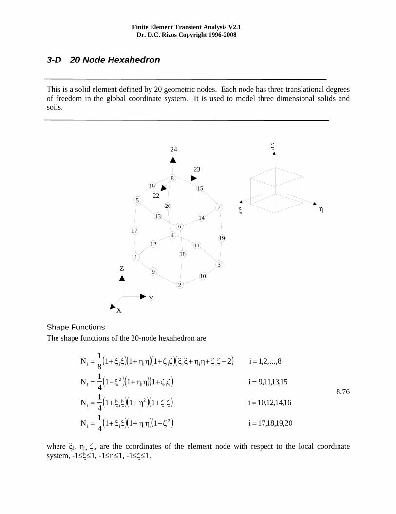
3-D 20 Node Hexahedron This is a solid element defined by 20 geometric nodes. Each node has three translational degrees of freedom in the global coordinate system. It is used to model three dimensional solids and soils.
Shape Functions The shape functions of the 20-node hexahedron are
( )( )( )( )
( )( )( )
( )( )( )
( )( )( )
N i
N i
N i
N i
i i i i i i i
i i i
i i i
i i i
= + + + + + − =
= − + + =
= + + + =
= + + + =
18
1 1 1 2 1 8
14
1 1 1 9111315
14
1 1 1 1012 1416
14
1 1 1 171819
2
2
2
ξ ξ η η ζ ζ ξ ξ η η ζ ζ
ξ η η ζ ζ
ξ ξ η ζ ζ
ξ ξ η η ζ
,2,...,
, , ,
, , ,
, , ,20
8.76
where ξi, ηi, ζi, are the coordinates of the element node with respect to the local coordinate system, -1≤ξ≤1, -1≤η≤1, -1≤ζ≤1.
Z
XY
1
2
3
4
5
6
7
910
1112
13 14
1516
17
18
19
20 ξ η
ζ24
23
22
8
Finite Element Transient Analysis V2.1 Dr. D.C. Rizos Copyright 1996-2008
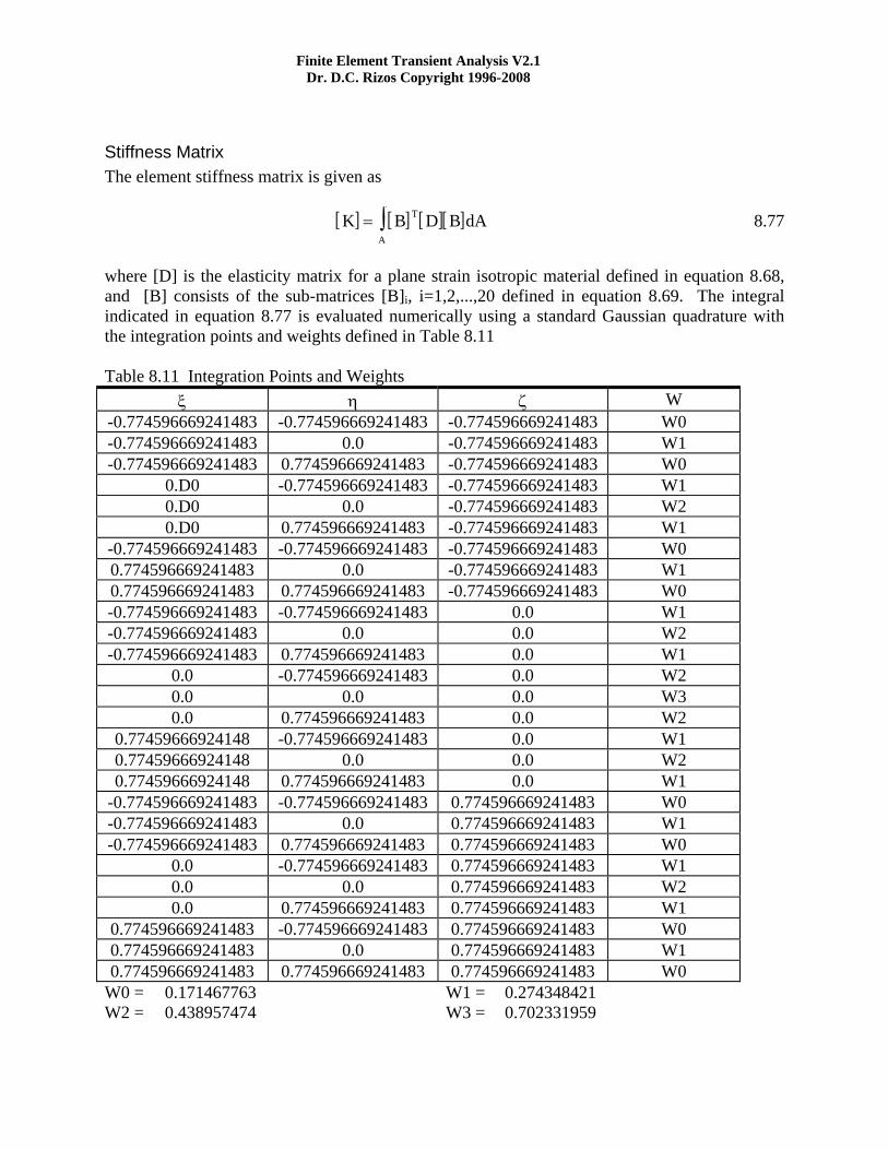
Stiffness Matrix The element stiffness matrix is given as
[ ] [ ] [ ][ ]K B D B dAT
A
= ∫ 8.77
where [D] is the elasticity matrix for a plane strain isotropic material defined in equation 8.68, and [B] consists of the sub-matrices [B]i, i=1,2,...,20 defined in equation 8.69. The integral indicated in equation 8.77 is evaluated numerically using a standard Gaussian quadrature with the integration points and weights defined in Table 8.11 Table 8.11 Integration Points and Weights
ξ η ζ W -0.774596669241483 -0.774596669241483 -0.774596669241483 W0 -0.774596669241483 0.0 -0.774596669241483 W1 -0.774596669241483 0.774596669241483 -0.774596669241483 W0
0.D0 -0.774596669241483 -0.774596669241483 W1 0.D0 0.0 -0.774596669241483 W2 0.D0 0.774596669241483 -0.774596669241483 W1
-0.774596669241483 -0.774596669241483 -0.774596669241483 W0 0.774596669241483 0.0 -0.774596669241483 W1 0.774596669241483 0.774596669241483 -0.774596669241483 W0 -0.774596669241483 -0.774596669241483 0.0 W1 -0.774596669241483 0.0 0.0 W2 -0.774596669241483 0.774596669241483 0.0 W1
0.0 -0.774596669241483 0.0 W2 0.0 0.0 0.0 W3 0.0 0.774596669241483 0.0 W2
0.77459666924148 -0.774596669241483 0.0 W1 0.77459666924148 0.0 0.0 W2 0.77459666924148 0.774596669241483 0.0 W1
-0.774596669241483 -0.774596669241483 0.774596669241483 W0 -0.774596669241483 0.0 0.774596669241483 W1 -0.774596669241483 0.774596669241483 0.774596669241483 W0
0.0 -0.774596669241483 0.774596669241483 W1 0.0 0.0 0.774596669241483 W2 0.0 0.774596669241483 0.774596669241483 W1
0.774596669241483 -0.774596669241483 0.774596669241483 W0 0.774596669241483 0.0 0.774596669241483 W1 0.774596669241483 0.774596669241483 0.774596669241483 W0
W0 = 0.171467763 W1 = 0.274348421 W2 = 0.438957474 W3 = 0.702331959

Finite Element Transient Analysis V2.1 Dr. D.C. Rizos Copyright 1996-2008 Mass Matrix The element mass matrix is evaluated on the basis of the consistent formulation as
[ ] [ ] [ ]M N N dAT
A
= ∫ρ 8.78
where ρ is the mass density of the elastic medium, and the integral is evaluated numerically, similarly to the stiffness matrix.
Damping Matrix For time domain analysis the damping matrix is evaluated according to the proportional damping formulation (Rayleigh damping) as a linear combination of the stiffness and mass matrices,
[ ] [ ] [ ]C a M b C= + 8.79
where a and b are user defined constants.

Finite Element Transient Analysis V2.1 Dr. D.C. Rizos Copyright 1996-2008
2-D Vertical Transmitting Boundaries The two dimensional vertical transmitting boundary is developed for frequency domain analysis. This elements are defined by all nodes bounding each side of the layered soil medium. They are used to model the far field motion of the infinite half space. These elements are attached directly to the finite elements of the soil region.
The element formulation is based on the calculation by the finite element method of the modes of vibration satisfying the boundary conditions on the surface and the bedrock. Subsequently, the solution in the far field is written as a linear combination of these semi-discrete modes. Details of this formulation can be found in the reference by J. Tassoulas and E. Kausel [8].
X
Y
Layer A
Layer B
Layer N
TransmittingBoundary
TransmittingBoundary

Finite Element Transient Analysis V2.1 Dr. D.C. Rizos Copyright 1996-2008
3-D Vertical Transmitting Boundaries The two dimensional vertical transmitting boundary is developed for frequency domain analysis. These elements are defined by all nodes on the surface of the soil cylinder. They are used to model the far field motion of the 3-D infinite half space. These elements are attached directly to the finite elements of the soil region. The three dimensional hyperelement is a direct extension of the two dimensional one introduced in the previous section. The development of this element by Lin and Tassoulas [3] who extended the axisymmetric boundaries of Waas [4] and Kausel [5] provides the basis for the hyperelement implemented in FETA. The approximate treatment of the half space underlying a layered stratum for both 2-D and 3-D is due to Hull and Kausel [6].

Finite Element Transient Analysis V2.1 Dr. D.C. Rizos Copyright 1996-2008
2-D Absorbing Boundary The two dimensional absorbing boundary is developed for time or frequency domain analysis. This elements are defined on the boundaries of the layered soil medium and consist of two or three nodes, depending on the soil elements that they are attached to. They are used to model the far field motion of the infinite half space by introducing appropriate dashpots. These elements are assembled directly to the damping matrix of the system under consideration.
Damping Matrix The absorbing boundary consists of vertical and horizontal dashpots per unit length of the boundary. The associated damping coefficients are proportional to the pressure, V1, and shear, V2 ,wave velocities and are evaluated as
C VC V
V
H
==
ρρ
1
2 8.80
The damping matrix is evaluated according to the consistent formulation.
X
Y

Finite Element Transient Analysis V2.1 Dr. D.C. Rizos Copyright 1996-2008
3-D Absorbing Boundary The three dimensional absorbing boundary is developed for time or frequency domain analysis. This elements are defined on the boundary of the layered soil medium and consist of six or eight nodes, depending on the soil elements they are attached to. They are used to model the far field motion of the infinite half space by introducing appropriate dashpots. These elements are assembled directly to the damping matrix of the system under consideration.
Damping Matrix The absorbing boundary consists of one vertical and two horizontal dashpots per unit length of the boundary. The associated damping coefficients are proportional to the pressure, V1, and shear, V2 ,wave velocities and are evaluated as
C VC V
V
H
==
ρρ
1
2 8.81
The damping matrix is evaluated according to the consistent formulation.
Y
Z

Finite Element Transient Analysis V2.1 Dr. D.C. Rizos Copyright 1996-2008
2-D Rigid Link The two dimensional rigid link is defined by two geometric nodes. This element implements the constrained equations for the motion of the two nodes in all corresponding degrees of freedom. Each node has two sets of two translational and one rotational degrees of freedom in the global coordinate system. The first set corresponds to displacements, and the second one corresponds to forces. In addition, a reference node, R, is assigned the three degrees of freedom shown in the figure to implement the coupling of the motion of the two geometric nodes. This element can be used by itself when both nodes have all three degrees of freedom, or combined with a massless 2-D beam element, that provides the appropriate stiffness, in any other case.
Constrained matrix The constrained matrix is formulated on the basis of the Lagrange multipliers, and for the 2-D rigid link element is given as:
Y
X
7,10
8,11
9,12
1,4
2,5
3,6 13
14
15R
1
2

Finite Element Transient Analysis V2.1 Dr. D.C. Rizos Copyright 1996-2008
[ ]L
RR
RR
symm
y
x
y
x=
−−
−−
− −−
−
⎡
⎣
⎢⎢⎢⎢⎢⎢⎢⎢⎢⎢⎢⎢
0 0 0 1 0 0 0 0 0 0 0 0 0 0 00 0 0 1 0 0 0 0 0 0 0 0 0 0
0 0 0 1 0 0 0 0 0 0 0 0 00 0 0 0 0 0 0 0 0 1 0 1
0 0 0 0 0 0 0 0 0 1 10 0 0 0 0 0 0 0 0 1
0 0 0 1 0 0 1 0 20 0 0 1 0 0 1 2
0 0 0 1 0 0 10 0 0 0 0 0
0 0 0 0 00 0 0 0
0 0 00 0
0
⎢⎢⎢⎢⎢⎢⎢⎢⎢⎢
⎤
⎦
⎥⎥⎥⎥⎥⎥⎥⎥⎥⎥⎥⎥⎥⎥⎥⎥⎥⎥⎥⎥⎥⎥ 8.82
where R1x=XR-X1, R1y=YR-Y1, R2x=XR-X2, and R2y=YR-Y2.

Finite Element Transient Analysis V2.1 Dr. D.C. Rizos Copyright 1996-2008
3-D Rigid Link
The three dimensional rigid link is defined by two geometric nodes. This element implements the constrained equations for the motion of the two nodes in all corresponding degrees of freedom. Each node has two sets of three translational and three rotational degrees of freedom in the global coordinate system. The first set corresponds to displacements, and the second one corresponds to forces. In addition, a reference node, R, is assigned the six degrees of freedom shown in the figure to implement the coupling of the motion of the two geometric nodes. This element can be used by itself when both nodes have all six degrees of freedom, or combined with a massless 3-D beam element, that provides the required stiffness, in any other case.
Y
X
1,7
2,8
3,9
R
1
2
Z
4,10
5,11
6,12
25
26
2728
29
30

Finite Element Transient Analysis V2.1 Dr. D.C. Rizos Copyright 1996-2008 Constrained matrix The constrained matrix is formulated on the basis of the Lagrange multipliers, and for the 3-D rigid link element is given as:
[ ]
[ ] [ ] [ ] [ ] [ ][ ] [ ] [ ] [ ] [ ]
[ ] [ ] [ ] [ ] [ ][ ] [ ] [ ] [ ] [ ][ ] [ ] [ ] [ ] [ ]
L
II L
II L
L LT T
=
−−
−−
⎡
⎣
⎢⎢⎢⎢⎢⎢
⎤
⎦
⎥⎥⎥⎥⎥⎥
0 0 0 00 0 0
0 0 0 00 0 00 0 0
1
2
1 2
8.83
where
[ ]L
R RR R
R Rwith
R X XR Y YR Z Z
z y
z x
y xx R
y R
z R
1
1
1
1
1 0 0 0 1 11 0 1 0 1
1 1 1 01 0 0
0 1 01
111
=
−−
−
⎡
⎣
⎢⎢⎢⎢⎢⎢⎢
⎤
⎦
⎥⎥⎥⎥⎥⎥⎥
= −= −= −
8.84
[ ]L
R RR R
R Rwith
R X XR Y YR Z Z
z y
z x
y xx R
y R
z R
2
2
2
2
1 0 0 0 2 21 0 2 0 2
1 2 2 01 0 0
0 1 01
222
=
−−
−
⎡
⎣
⎢⎢⎢⎢⎢⎢⎢
⎤
⎦
⎥⎥⎥⎥⎥⎥⎥
= −= −= −

Finite Element Transient Analysis V2.1 Dr. D.C. Rizos Copyright 1996-2008
2-D Rigid Footing The 2-D rigid footing consists of all geometric nodes in contact with the user defined line which represents the rigid region, and an additional reference node that enforces the rigid conditions. Each node in the rigid footing along with the common reference node becomes a 2-D rigid footing element and its formulation is based on the Lagrange multipliers. Each node has two sets of two translational degrees of freedom in the global coordinate system. The first set corresponds to displacements, and the second one corresponds to forces. The reference node has two translational and one rotational degrees of freedom corresponding to the translations and rotation of the footing as rigid body.
Constrained matrix The constrained matrix is formulated on the basis of the Lagrange multipliers, and for the 2-D rigid footing element is given as:
[ ]L
RR
R R
where R X X R Y Yy
x
y x
x R y R=
−−
−− −
−
⎡
⎣
⎢⎢⎢⎢⎢⎢⎢⎢⎢
⎤
⎦
⎥⎥⎥⎥⎥⎥⎥⎥⎥
= − = −
0 0 1 0 0 0 00 0 0 1 0 0 01 0 0 0 1 0
0 1 0 0 0 10 0 1 0 0 0 00 0 0 1 0 0 00 0 0 0 0
1 1, 8.85
Y
X
1,3
2,45
6
7R
1
N
n
m
iRigidLine
Rigid FootingElement

Finite Element Transient Analysis V2.1 Dr. D.C. Rizos Copyright 1996-2008
3-D Rigid Footing The 3-D rigid footing consists of all geometric nodes in contact with the user defined surface which represents the rigid region, and an additional reference node that enforces the rigid conditions. Each node in the rigid footing along with the common reference node becomes a 3-D rigid footing element and its formulation is based on the Lagrange multipliers. Each node has two sets of three translational degrees of freedom in the global coordinate system. The first set corresponds to displacements, and the second one corresponds to forces. The reference node has three translational and three rotational degrees of freedom corresponding to the translations and rotations of the footing as rigid body.
Constrained matrix The constrained matrix is formulated on the basis of the Lagrange multipliers, and for the 3-D rigid footing element is given as:
[ ]
[ ] [ ] [ ] [ ][ ] [ ] [ ] [ ]
[ ] [ ] [ ] [ ][ ] [ ] [ ] [ ]
L
II I R
IR T
=
−−
⎡
⎣
⎢⎢⎢⎢
⎤
⎦
⎥⎥⎥⎥
0 0 00
0 0 00 0 0
8.86
Y
X
RigidSurface
Rigid FootingElement
Z
1,4
2,5
3,67
89 10
11
12

Finite Element Transient Analysis V2.1 Dr. D.C. Rizos Copyright 1996-2008 where [I] is the identity matrix and
[ ]RR R
R RR R
z y
z x
y x
=−
−−
⎡
⎣
⎢⎢⎢
⎤
⎦
⎥⎥⎥
00
0 with
R X XR Y YR Z Z
x R n
y R n
z R n
= −= −
= −
8.87

Finite Element Transient Analysis V2.1 Dr. D.C. Rizos Copyright 1996-2008
2-D Frictional Contact Element The 2-D frictional contact element is an interface element between two bodies in contact. It consists of three pairs of nodes. The two nodes of each pair are initially coincident. Each node has two degrees of freedom in the local coordinate system, i.e. the tangential velocity and the normal displacement. In addition, three parameters are required to completely describe the element, i.e. the coefficient of friction μ, and the penalty coefficients kn, and ks that represent the relative stiffness in the normal and tangential direction, respectively. This element is used in time domain analysis only.
Formulation Parameters The sides of the element that may be in frictional contact are defined by nodes 1-3-5 and 2-4-6. Let ( ) ( ) ( )x u vi i i
~ ~ ~, , be the position, displacement and velocity vectors of node i. At any point s
along the element, we can compute
( ) ( ) ( ) ( ) ( ) ( )
( ) ( ) ( ) ( ) ( ) ( )
( ) ( ) ( ) ( ) ( ) ( )
x x N s x N s x N s
u u N s u N s u N s
u u N s u N s u N s
~ ~ ~ ~
~ ~ ~ ~
~ ~ ~ ~
= + +
= + +
= + +
+
−
11
32
53
21
42
63
11
32
53
8.88
Y
X
1,2
3,4
5,6n s

Finite Element Transient Analysis V2.1 Dr. D.C. Rizos Copyright 1996-2008
( ) ( ) ( ) ( ) ( ) ( )
( ) ( ) ( ) ( ) ( ) ( )
v v N s v N s v N s
v v N s v N s v N s~ ~ ~ ~
~ ~ ~ ~
+
−
= + +
= + +
21
42
63
11
32
53
where Ni are the quadratic Lagrangian interpolation functions. In terms of the above we can determine the unit vectors, tangent and normal to the element:
sss n
nn
ss
x
y
x
y
y
x~ ~=
⎧⎨⎩
⎫⎬⎭
=⎧⎨⎩
⎫⎬⎭
=−⎧
⎨⎩
⎫⎬⎭
8.89
The separation and relative tangential velocity are then given by:
δn
T
s
T
u u n
v v v s
= −⎛⎝⎜
⎞⎠⎟
= −⎛⎝⎜
⎞⎠⎟
+ −
+ −
~ ~ ~
~ ~ ~
8.90
where negative δn indicates penetration. Finally, the forces on the interface nodes are computed as: If δn≤ε
F k
F
k v ifF
kv
Fk
F if vF
k
F if vF
k
n n n
s
s sn
ss
n
s
n sn
s
n sn
s
=
=
− ≤ ≤
>
− < −
⎧
⎨
⎪⎪⎪⎪
⎩
⎪⎪⎪⎪
δ
μ μ
μμ
μμ
8.91 If δn>ε
FF
n
s
==
00
where kn and ks are the penalty parameters indicating the relative stiffness between the two bodies and ε is a positive tolerance.

Finite Element Transient Analysis V2.1 Dr. D.C. Rizos Copyright 1996-2008 Stiffness Matrix The contribution to the stiffness matrix is evaluated as
[ ] [ ] [ ] [ ] [ ]K N Q D Q N dsTn n n
T
s= ∫ 8.91
where
[ ] [ ] [ ] [ ] [ ] [ ] [ ][ ] [ ]N N N N N N N NN
Nii
i= − − − =
⎡
⎣⎢
⎤
⎦⎥1 1 2 2 3 3
00
8.92
are the shape functions, Qn contains the directional cosines of the normal and
Dk if
otherwisenn n=
≤⎧⎨⎩
δ ε0
8.93
Damping Matrix The contribution of the element in the damping matrix of the system is calculated as
[ ] [ ] [ ] [ ] [ ]C N Q D Q N dsTs s s
T
s= ∫ 8.94
where [N] are the shape functions as in Equation 8.02, Qs contains the directional cosines of the tangent vector and
Dk if and v
Fk
otherwises
s n sn
s=≤ ≤
⎧
⎨⎪
⎩⎪
δ εμ
0 8.95
Contribution to the Right Hand Side The contribution to the right hand side of the system of equations is calculated as
{ } [ ] [ ][ ]R N Q F dsT
s= −∫ 8.96
where [N] are the shape functions as indicated in Equation 8.02, [Q] contains the directional cosines and {F} is the vector of the forces on the frictional interface as calculated in equation 8.91.

Finite Element Transient Analysis V2.1 Dr. D.C. Rizos Copyright 1996-2008
28 2-D Fluid Element The 2-D fluid element is developed on the basis of the Helmholtz’s or Laplace’s equation for the time harmonic motion of compressible and incompressible fluids, respectively. It is a 2-D 3-node or 4-node surface patch element and the degrees of freedom correspond to the fluid velocity potential. Along with the fluid-solid interface is used to model fluid domains in a fluid-structure-interaction applications.
Formulation The governing equation for time harmonic motion of a compressible fluid is the well known Helmholtz’s equation:
∂ φ
∂
∂ φ
∂
ωφ
2
2
2
2
2
2 0x y C
+ + = 8.97
while the Laplace’s equation
∂ φ
∂
∂ φ
∂
2
2
2
2 0x y
+ = 8.98
must be satisfied in an incompressible fluid. In equations 8.97 and 8.98, φ denotes the fluid velocity potential and C is the pressure wave velocity. Applying the variational approach, both sides of equation 8.97 are multiplied by ρδφ and integrated by parts over the domain Ω. This approach yields:
Y
X
1
3
2 1
4 3
2

Finite Element Transient Analysis V2.1 Dr. D.C. Rizos Copyright 1996-2008
( ) ( ) ( )− +⎡
⎣⎢
⎤
⎦⎥ + =
−⎛⎝⎜
⎞⎠⎟+
⎛
⎝⎜
⎞
⎠⎟
⎡
⎣⎢
⎤
⎦⎥
∫ ∫
∫
ρ∂ δφ
∂∂φ∂
∂ δφ∂
∂φ∂
ωρ δφ φ
ρ∂
∂δφ
∂φ∂
∂∂
δφ∂φ∂
x x y yd
Cd
x x y yd
Ω Ω
Ω
Ω Ω
Ω
2
2
8.99
Applying Green’s theorem on the right hand side of equation 8.99 in order to change the integral over the domain Ω to the integral over the domain B yields:
( ) ( ) ( )− +⎡
⎣⎢
⎤
⎦⎥ + =
− +⎛
⎝⎜
⎞
⎠⎟
∫ ∫
∫
ρ∂ δφ
∂∂φ∂
∂ δφ∂
∂φ∂
ωρ δφ φ
ρ δϕ∂φ∂
∂φ∂
x x y yd
Cd
xn
yn dBx y
B
Ω ΩΩ Ω
2
2
8.100
Considering triangular, or quadrilateral isoparametric elements with linear interpolation of the amplitude of the velocity potential equation 8.100 can be written as:
−⎛⎝⎜
⎞⎠⎟⎛⎝⎜
⎞⎠⎟ +
⎛⎝⎜
⎞⎠⎟⎛⎝⎜
⎞⎠⎟
⎡
⎣⎢⎢
⎤
⎦⎥⎥
+
+
⎡
⎣
⎢⎢⎢⎢⎢⎢⎢
⎤
⎦
⎥⎥⎥⎥⎥⎥⎥
⎧
⎨
⎪⎪⎪
⎩
⎪⎪⎪
⎫
⎬
⎪⎪⎪
⎭
⎪⎪⎪
=
⎧
⎨
⎪⎪⎪
⎩
⎪⎪⎪
⎫
⎬
⎪⎪⎪
⎭
⎪⎪⎪
∫
∫
ρ∂∂
∂∂
∂∂
∂∂
ωρ
φ
Nx
Nx
N N
NN T
T T
i iy y
d
Cd
RΩ
Ω
Ω
Ω
2
2
8.101
where N = Ni, i=1,.. number of element nodes, is the vector of the shape functions associated to the element that is used (see equations 8.48, 8.58), φi is the velocity potential at the nodes of the element, and
R Nx
ny
n dBi i x yB
= − +⎛⎝⎜
⎞⎠⎟∫ρ
∂φ∂
∂φ∂
8.102
represents the amplitude of the consistent mass flux into the domain at node i. In the case of an incompressible fluid, the second integral in equation 8.1015 will drop out.

Finite Element Transient Analysis V2.1 Dr. D.C. Rizos Copyright 1996-2008
2-D Fluid-Solid Interface Element The 2-D fluid-solid interface element is an element that relates the nodal velocity potentials of the fluid region to the nodal horizontal and vertical displacements of the solid domain. This element is created automatically by FETA at the interface between fluid and solid domains and is invisible to the user.
Y
X
1
2Fluid
Solid
φ1
φ2
U1,W1
U2,W2
Formulation At the interface between the fluid and solid finite elements, the nodal velocity potentials of fluid must be related to the nodal horizontal and vertical displacements of the solid finite element. This can be done by taking the contributions of the consistent mass flux, and consistent nodal forces on the common boundary S to the left-hand side of the equations and for convenience storing the result as a matrix of an auxiliary interface element to be assembled with the matrices corresponding to the solid and fluid finite elements. The contribution of the mass flux through S corresponding to the starting (1) and ending (2) nodes of the interface element are given explicitly after integration in terms of the outward normal and the horizontal and vertical displacements U and W as

Finite Element Transient Analysis V2.1 Dr. D.C. Rizos Copyright 1996-2008
R i Ln n n n
UWUW
R i Ln n n n
UWUW
S x y x y
S x y x y
1
1
1
2
2
2
1
1
2
2
3 3 6 6
6 6 3 3
= −⎡
⎣⎢
⎤
⎦⎥
⎡
⎣
⎢⎢⎢⎢
⎤
⎦
⎥⎥⎥⎥
= −⎡
⎣⎢
⎤
⎦⎥
⎡
⎣
⎢⎢⎢⎢
⎤
⎦
⎥⎥⎥⎥
ωρ
ωρ
8.103
On the other hand, the contribution of the consistent horizontal and vertical nodal forces H and V from S to the starting (1) and ending (2) nodes of the interface element are given explicitly after integration in terms of the fluid pressure on S as:
H i Ln n
V i Ln n
H i Ln n
V i Ln n
S x x
S y y
S x x
S y y
11
2
11
2
21
2
21
2
3 6
3 6
6 3
6 3
= −⎡⎣⎢
⎤⎦⎥⎡
⎣⎢
⎤
⎦⎥
= −⎡
⎣⎢
⎤
⎦⎥⎡
⎣⎢
⎤
⎦⎥
= −⎡⎣⎢
⎤⎦⎥⎡
⎣⎢
⎤
⎦⎥
= −⎡
⎣⎢
⎤
⎦⎥⎡
⎣⎢
⎤
⎦⎥
ωρφφ
ωρφφ
ωρφφ
ωρφφ
8.104
The relations 8.103 and 8.104 represent the contributions of the consistent mass flux and consistent nodal forces on the interface S. If these contributions are taken to the left-hand side of the equations, the matrix of the auxiliary element is formed as:
Q =
⎡
⎣
⎢⎢⎢⎢⎢⎢⎢⎢⎢⎢⎢⎢⎢⎢
⎤
⎦
⎥⎥⎥⎥⎥⎥⎥⎥⎥⎥⎥⎥⎥⎥
i L
n n n n
n n n n
n n
n n
n n
n n
x y x y
x y x y
x x
y y
x x
y y
ωρ
0 03 3 6 6
0 06 6 3 3
3 60 0 0 0
3 60 0 0 0
6 30 0 0 0
6 30 0 0 0
8.105
Clearly this matrix is symmetric. Thus, an element has been formulated with degrees of freedom [ ]φ φ1 2 1 1 2 2U W U W . Inserting such elements along the soil-fluid interface, the usual

Finite Element Transient Analysis V2.1 Dr. D.C. Rizos Copyright 1996-2008 solid and fluid elements can be used without any modifications. Detailed formulation can be found in the reference by Lotfi and Tassoulas [7].

Finite Element Transient Analysis V2.1 Dr. D.C. Rizos Copyright 1996-2008


