Finite element simulation of microphotonic lasing...

Finite element simulation ofmicrophotonic lasing system

Chris Fietz1k∗ and Costas M. Soukoulis1,2

1Ames Laboratory and Department of Physics and Astronomy, Iowa State University, Ames,Iowa 50011, USA

2Institute of Electronic Structure and Laser, FORTH, 71110 Heraklion, Crete, Greece∗[email protected]

Abstract: We present a method for performing time domain simulationsof a microphotonic system containing a four level gain medium based onthe finite element method. This method includes an approximation thatinvolves expanding the pump and probe electromagnetic fields around theirrespective carrier frequencies, providing a dramatic speedup of the timeevolution. Finally, we present a two dimensional example of this model,simulating a cylindrical spaser array consisting of a four level gain mediuminside of a metal shell.

© 2012 Optical Society of AmericaOCIS codes: (160.3918) Metamaterials; (140.3460) Lasers; (050.1755) Computational elec-tromagnetic methods.

References and links1. K. Bohringer and O. Hess, “A full time-domain approach to spatio-temporal dynamics of semiconductor lasers.

II. spatio-temporal dynamics,” Prog. Quantum Electron.32, 247–307 (2008).2. A. Fang, T. Koschny, M. Wegener, and C. M. Soukoulis, “Self-consistent calculation of metamaterials with gain,”

Phys. Rev. B79, 241104 (2009).3. A. Fang, “Reducing the losses of optical metamaterials,” Ph.D. thesis, Iowa State University (2010).4. A. Fang, T. Koschny, and C. M. Soukoulis, “Lasing in metamaterial nanostructures,” J. Opt.12, 024013 (2010).5. A. Fang, T. Koschny, and C. M. Soukoulis, “Self-consistent calculations of loss-compensated fishnet metamate-

rials,” Phys. Rev. B82, 121102 (2010).6. S. Wuestner, A. Pusch, K. L. Tsakmakidis, J. M. Hamm, and O. Hess, “Overcoming losses with gain in a negative

refractive index metamaterial,” Phys. Rev. Lett.105, 127401 (2010).7. A. Fang, Z. Huang, T. Koschny, and C. M. Soukoulis, “Overcoming the losses of a split ring resonator array with

gain,” Opt. Express19, 12688–12699 (2011).8. S. Wuestner, A. Pusch, K. L. Tsakmakidis, J. M. Hamm, and O. Hess, “Gain and plasmon dynamics in active

negative-index metamaterials,” Phil. Trans. R. Soc. London Ser. A369, 3525–3550 (2011).9. J. M. Hamm, S. Wuestner, K. L. Tsakmakidis, and T. Hess, “Theory of light amplification in active fishnet

metamaterials,” Phys. Rev. Lett.107, 167405 (2011).10. J. A. Gordon and R. W. Ziolkowski, “The design and simulated performance of a coated nano-particle laser,”

Opt. Express15, 2622–2653 (2007).11. J. A. Gordon and R. W. Ziolkowski, “CNP optical metamaterials,” Opt. Express16, 6692–6716 (2008).12. A. E. Siegman,Lasers(University Science Books, 1986). See chapters 2, 3, and 6.13. X. Jiang and C. M. Soukoulis, “Time dependent theory for random lasers,” Phys. Rev. Lett.85, 70–73 (2000).14. W. B. J. Zimmerman,Process Modelling and Simulation with Finite Element Methods(World Scientific, 2004).15. J. Jin,The Finite Element Method in Electromagnetics, 2nd ed. (John Wiley & Sons, Inc., 2002).16. D. J. Bergman and M. I. Stockman, “Surface plasmon amplification by stimulated emission of radiation: quantum

generation of coherent surface plasmons in nanosystems,” Phys. Rev. Lett.90, 027402 (2003).17. M. I. Stockman, “Spasers explained,” Nat. Photon.2, 327–329 (2008).18. E. F. Kuester, M. A. Mohamed, M. Piket-May, and C. L. Holloway, “Averaged transition conditions for electro-

magnetic fields at a metafilm,” IEEE Trans. Antennas Propag.51, 2641–2651 (2003).19. C. Fietz and G. Shvets, “Homogenization theory for simple metamaterials modeled as one-dimensional arrays of

thin polarizable sheets,” Phys. Rev. B82, 205128 (2010).

#166283 - $15.00 USD Received 9 Apr 2012; revised 27 Apr 2012; accepted 30 Apr 2012; published 4 May 2012(C) 2012 OSA 7 May 2012 / Vol. 20, No. 10 / OPTICS EXPRESS 11548

1. Introduction

Interestin microphotonic lasing systems has been increasing over the past few years. As a re-sult, it has become more important to be able to numerically simulate these lasing systems.Several finite difference time domain (FDTD) simulations of a four level gain medium embed-ded in a microphotonic system have been presented previously [1–9], but these simulations alluse structured (cubic) grids and consequently accurately model curved geometries. There havealso been methods developed to model spherical gain geometries by expanding electromagneticfields as sums of spherical Bessel functions [10, 11]. These methods overcome the limitationsof structured grids for spherical geometries, but in turn are limited to only modelling sphericalgeometries. In principle it should be possible to model a microphotonic lasing system with anFDTD simulation utilizing unstructured grids, but to the best knowledge of the authors this hasnot been demonstrated. The finite element method (FEM) can utilize unstructured grids and asa result can model a wide variety of geometries. In this paper we present a FEM model of amicrophotonic system with gain arising from a four level quantum system. In addition to devel-oping a FEM microphotonic lasing model, an approximation is introduced whereby the pumpand probe fields are solved for separately, with each field described by the slowly varying com-plex valued field amplitude of a constant frequency carrier wave. This approximation allowsfor much larger time steps and a considerable speedup in simulation time.

In the first section of this paper we will describe the dynamics of the microphotonic lasingsystem, the carrier wave approximation, and finally the finite element formulation of the prob-lem. In the second section we present a two dimensional model of a one dimensional cylindricalspaser array as an example of this new simulation method.

2. FEM microphotonic lasing simulation

2.1. Field equations of a microphotonic lasing system

The simulation we present of a microphotonic lasing system requires the time domain mod-elling of several different fields and their mutual interactions. These fields include the electro-magnetic field, the electric polarization field inside a metal with a Drude response, the electricpolarization field of the gain medium, and the population density fields of the different energylevels of the gain medium. Each of these fields evolve according a particular differential equa-tion that must be solved when simulating a microphotonic lasing system. The field equation forthe electromagnetic field is

∇×(

1µ0

∇×A)

+ εrε0∂ 2A∂ t2 =

∂P∂ t

, (1)

whereA is the electromagnetic vector potential,P is a polarization vector describing either aDrude response from a metal inclusion or a Lorentzian response from a four level gain system,andεr is a relative permittivity that is constant with respect to frequency and not included inP.Here and for the remainder of the paper we have use SI units. Also, we have used the tempo-ral gauge condition∂A0/∂ t = 0 along with the initial condition for the electrostatic potentialA0(t = 0,x) = 0 to ensure that the electrostatic potential is zero for all time, eliminating it fromour equations. Given this choice of gauge the electric field and magnetic flux density are definedas

E = −∂A∂ t

,

B = ∇×A

(2)


Using this definition forE, the Drude response of a metal inclusion is determined by the equa-tion

∂P∂ t

+ γP = −ε0ω2pA (3)

whereωp is the plasma frequency andγ is the damping frequency of the Drude metal.

0

1

2

3

ωb ωa

τ30 τ32

τ21

τ10

Fig. 1. Simple model of a four level gain medium. The lasing and pump transitions areassumedto be electric dipole transistions with frequencies ofωa andωb respectively. Thedecay processes between the i-th and j-th energy levels are described by the decay rates1/τi j .

The gain medium is modelled as simple four level quantum system, described schematicallyin Fig. 1. The 1→ 2 transition is an electric dipole transition with a frequency ofωa. Similarly,the 0→ 3 transition is also an electric dipole transition with frequencyωb. Spontaneous decaybetween the i-th level to the j-th level occurs at the decay rate of 1/τi j . These decay ratesinclude both radiative (spontaneous photon emission) and non-radiative (spontaneous phononemission) decay processes. In the case of spontaneous photon emission, our model does notproduce a photon. Coupling of the gain medium to the electromagnetic field is only allowed forstimulated photon emission.

The electromagnetic response of the four level gain system is given by

∂ 2Pai

∂ t2 +Γa∂Pai

∂ t+ω2

aPai = −σa(N2i −N1i)Ei ,

∂ 2Pbi

∂ t2 +Γb∂Pbi

∂ t+ω2

bPbi = −σb(N3i −N0i)Ei .

(4)

Here Pai and Pb

i are the i-th components of the gain polarization due to transitions between the1st and 2nd levels and between the 0th and 3rd levels respectively. Additionally,Γa andΓb arethe linewidths of these transitions,σa andσb are coupling constants, and N0i , N1i , N2i and N3i

are the population number densities for oscillators polarized in the i-th direction for the 0th, 1st,2nd and 3rd energy levels. Note thatΓa ≥ 1/τ21 andΓb ≥ 1/τ30 [12].

Finally, the population number densities evolve according the equations [12,13]


∂N3i

∂ t=

1hωb

Ei∂Pbi

∂ t−(

1τ30

+1

τ32

)

N3i ,

∂N2i

∂ t=

N3i

τ32+

1hωa

Ei∂Pai

∂ t−

N2i

τ21,

∂N1i

∂ t=

N2i

τ21−

1hωa

Ei∂Pai

∂ t−

N1i

τ10,

∂N0i

∂ t=

N3i

τ30+

N1i

τ10−

1hωb

Ei∂Pbi

∂ t,

(5)

Together, this system of equations (Eqs. (1), (3)–(5)) completely describes the dynamics ofthe microphotonic lasing system. The main disadvantage of solving this system of differen-tial equations is the small time step required. In practice,∼ 100 time steps per period of thepumping laser beam are required for an adequate simulation. A typical lasing simulation couldrequire over 100,000 lasing periods, making the computational requirements of the simulationprohibitively large.

2.2. Period averaged approximation

There is a simple method for dramatically speeding up the simulation time. The electromag-netic field as well as the polarization fields oscillates at two frequencies. These two frequenciesare approximately equal to the frequency of the 1→ 2 transition frequencyωa, and the 0→ 3transition frequencyωb. Much of the computational effort required in this time domain simu-lation is spent on these simple, approximately harmonic oscillations. A good approximation isto assume these fields oscillate harmonically, with complex valued amplitudes that are slowlychanging in time. We can ignore the fast oscillations and instead simulate the relatively slowertime dependence of these amplitudes.

Since there are two frequencies, we divide our electromagnetic field into two separate fields

A(t,x) =A1(t,x)eiω1t +A2(t,x)eiω2t +c.c.

2, (6)

with each field oscillating at a different frequency. HereA1 is the complex valued amplitude foran electromagnetic field that oscillates at a frequency close to the 1→ 2 transition (ω1 ≈ ωa),andA2 is the complex valued amplitude for an electromagnetic field that oscillates close to the0→ 3 transition (ω2 ≈ ωb). Also,c.c. indicates the complex conjugate of the preceding terms.

By inserting the above equation into Eq. (1), the field equation forA, we derive two new fieldequations

∇×(

1µ0

∇×A1

)

+ εrε0

(

−ω21A1 +2iω1

∂A1

∂ t+

∂ 2A1

∂ t2

)

=∂P1

∂ t,

∇×(

1µ0

∇×A2

)

+ εrε0

(

−ω22A2 +2iω2

∂A2

∂ t+

∂ 2A2

∂ t2

)

=∂P2

∂ t.

(7)

Here we have also separated the polarization field into two fields

P(t,x) =P1(t,x)eiω1t +P2(t,x)eiω2t +c.c

2. (8)

For Drude metal inclusions the polarization fields obey the equations


iω1Pd1 +

∂Pd1

∂ t+ γPd

1 = −ε0ω2pA1,

iω2Pd2 +

∂Pd2

∂ t+ γPd

2 = −ε0ω2pA2,

(9)

while for Lorentzian gain inclusions the polarization fields obey the equations

−ω21Pg

1i +2iω1∂Pg

1i

∂ t+

∂ 2Pg1i

∂ t2 +Γa

(

iω1Pg1i +

∂Pg1i

∂ t

)

+ω2aPg

1i = −σa (N2i −N1i)E1i ,

−ω22Pg

2i +2iω2∂Pg

2i

∂ t+

∂ 2Pg2i

∂ t2 +Γb

(

iω2Pg2i +

∂Pg2i

∂ t

)

+ω2bPg

2i = −σb (N3i −N0i)E2i .

(10)

Here E1i and E2i are the i-th components of the electric fields associated with the potentialsA1

andA2, and are defined asE1 = −∂A1/∂ t andE2 = −∂A1/∂ t respectively.Finally, the new differential equations for the occupation number densities are

∂N3i

∂ t=

1hωb

⟨

E2i∂P2i

∂ t

⟩

−(

1τ30

+1

τ32

)

N3i ,

∂N2i

∂ t=

N3i

τ32+

1hωa

⟨

E1i∂P1i

∂ t

⟩

−N2i

τ21,

∂N1i

∂ t=

N2i

τ21−

1hωa

⟨

E1i∂P1i

∂ t

⟩

−N1i

τ10,

∂N0i

∂ t=

N3i

τ30+

N1i

τ10−

1hωb

⟨

E2i∂P2i

∂ t

⟩

.

(11)

Here the coupling term between the occupation number density fields and the electromagneticand polarization fields has been replaced by a term representing the period averaged value ofthese terms

⟨

E1i∂P1i

∂ t

⟩

=12

Re

[(

−iω1A1i −∂A1i

∂ t

)∗(

iω1P1i +∂P1i

∂ t

)]

,

⟨

E2i∂P2i

∂ t

⟩

=12

Re

[(

−iω1A2i −∂A2i

∂ t

)∗(

iω1P2i +∂P2i

∂ t

)]

,

(12)

where∗ indicates complex conjugation.Finally, we mention that while we have developed the preceding approximation using a FEM

model, this approximation is not limited to the FEM. It could potentially be used to speedupboth the FDTD models of microphotonic lasing systems [1–9] as well as the time domainmodels of spherical lasing geometries utilizing spherical Bessel functions [10,11].

2.3. Finite element formulation

Now that we have derived the period averaged field equations (Eqs. (7), (9)–(12)) for the mi-crophotonic lasing system, we can convert these differential equations into weak forms that canbe solved in a finite element simulation.


The weak forms for the field equations of the electromagnetic fields (Eq. (7)) are

FA1(A1,A1) =(

∇× A1)

·1µ0

(∇×A1)+ εrε0A1 ·(

−ω21A1 +2iω1

∂A1

∂ t+

∂ 2A1

∂ t2

)

−A1 ·∂P1

∂ t,

FA2(A2,A2) =(

∇× A2)

·1µ0

(∇×A2)+ εrε0A2 ·(

−ω22A2 +2iω2

∂A2

∂ t+

∂ 2A2

∂ t2

)

−A2 ·∂P2

∂ t.

(13)

Here∼ indicates a test function [14, 15]. These weak forms enforce both the electromagneticfield equations as well as a natural boundary condition [14, 15]. The finite element methodrequires that the integral of the weak form over the simulation domain be set to zero. As anexample, if we apply this requirement to the weak form FA1, we find that by integrating byparts we obtain a volume integral enforcing the electromagnetic field equation as well as asecond boundary integral enforcing a boundary condition on the field,

0 =

∫

Ωd3x FA1

=∫

Ωd3x A1 ·

[

∇×(

1µ0

∇×A1

)

+ εrε0

(

−ω21A1 +2iω1

∂A1

∂ t+

∂ 2A1

∂ t2

)

−∂P1

∂ t

]

−∮

∂ΩdA A1 ·

[

n×(

1µ0

∇×A1

)]

.

(14)Here Ω is the simulation domain,∂Ω is the boundary of that domain,dA is a infinitesimaldifferential area on that boundary, andn is the direction normal to the boundary. In the absenceof any extra boundary terms, the boundary integral in Eq. (14) forces the tangential componentof the magnetic fieldH1 to zero. Thisperfect magnetic conductorboundary condition is notdesirable for our simulation, so we will modify it to allow for a boundary that absorbs andemits plane waves at normal incidence to the boundary.

For a flat boundary at a large enough distance from the inclusions in the simulation domainthat evanescent waves are negligibly small, if the remaining propagating fields are normal to thisflat boundary then the vector potential can be represented as the sum of two vector potentials,

A1(t,x) = a(

t −n ·x

c

)

+b(

t +n ·x

c

)

. (15)

Herea is the vector potential of a plane wave propagating toward the boundary andb is thevector potential of a plane wave propagating away from the boundary. The boundary conditionwe desire is one that absorbsa and emits an arbitrarily definedb. If we take the part of thesurface integrand from Eq. (14) that is within the brackets and substitute Eq. (15) forA1 we get


n×(

1µ0

∇×A1

)

= n×(

−n

µ0c×

∂a∂ t

+n

µ0c×

∂b∂ t

)

=1z0

(

n× n×(

Eout1 −Einc

1

)

)

= −1z0

n× n×(

∂A1

∂ t+2Einc

1

)

,

(16)

whereEout1 = −∂a/∂ t is the part of the electric field associated the plane wavea propagating

toward the boundary, andEinc1 = −∂b/∂ t is the part of the electric field associated with the

plane waveb propagating away from the boundary, the sum of which isEout1 + Einc

1 = E1 =

−∂A1/∂ t. Also, z0 ≡√

µ0/ε0 is the impedance of free space. Multiplying Eq. (16) by a testfunctionA1 and integrating over the domain boundary gives us a new boundary weak term

BA1(A1,A1) = −∮

∂ΩdA

1z0

A1 ·[

n× n×(

∂A1

∂ t+2Einc

1

)]

. (17)

Adding this additional boundary weak term to specific boundaries enforces amatched boundarycondition(referred to as anabsorbing boundary conditionin Ref. [15]) which allows for planewaves normal to the boundary to be absorbed and for the incident plane waveEinc

1 to be emittedinto the domain normal to the boundary. A matched boundary condition forA2 can be enforcedin the same manner.

The weak forms for the remaining field equations are simpler since these differential equa-tions only involve derivatives with respect to time. The weak form for the polarization of Drudemetal inclusions is

FPD1(Pd1,P

d1) = Pd

1 ·[

iω1Pd1 +

∂Pd1

∂ t+ γPd

1 + ε0ω2pA1

]

,

FPD2(Pd2,P

d2) = Pd

2 ·[

iω2Pd2 +

∂Pd2

∂ t+ γPd

2 + ε0ω2pA2

]

,

(18)

where again a∼ indicates a test function. Similarly, the weak form for the polarization fieldsof the gain medium are

FPG1(Pg1,P

g1) = Pg

1 ·[

−ω21Pg

1i +2iω1∂Pg

1i

∂ t+

∂ 2Pg1i

∂ t2 +Γa

(

iω1Pg1i +

∂Pg1i

∂ t

)

+ω2aPg

1i +σa (N2i −N1i)E1i

]

,

FPG2(Pg2,P

g2) = Pg

2 ·[

−ω22Pg

2i +2iω2∂Pg

2i

∂ t+

∂ 2Pg2i

∂ t2 +Γb

(

iω2Pg2i +

∂Pg2i

∂ t

)

+ω2bPg

2i +σb (N3i −N0i)E2i

]

,

(19)

and the weak forms for the population density rate equations are


FN3i(N3i ,N3i) = N3i ·[

∂N3i

∂ t−

1hωb

⟨

E2i∂P2i

∂ t

⟩

+

(

1τ30

+1

τ32

)

N3i

]

,

FN2i(N2i ,N2i) = N2i ·[

∂N2i

∂ t−

N3i

τ32−

1hωa

⟨

E1i∂P1i

∂ t

⟩

+N2i

τ21

]

,

FN1i(N1i ,N1i) = N1i ·[

∂N1i

∂ t−

N2i

τ21+

1hωa

⟨

E1i∂P1i

∂ t

⟩

+N1i

τ10

]

,

(20)

where the period averaged values for the coupling term are given in Eq. (12). Also, we canavoid solving for N0i by taking advantage of the fact that N0i = Nint −N1i −N2i −N3i whereNint is the initial value of N0i when N1i = N2i = N3i = 0.

3. Cylindrical spaser array

As an example of a microphotonic lasing system simulation we present a two dimensionalmodel of a spaser (surface plasmon amplification by stimulated emission of radiation [16,17]).The time domain FEM simulation was performed using the commercial software COMSOLMultiphysics 3.5. For time stepping, the Generalized-α method was used with the dampingparameterρin f = 1. A copy of the model can be obtained by contacting the correspondingauthor by email.

The spaser is a one dimensional array of cylinders, each cylinder being infinite in extent intheir axial direction. Each cylinder has a core consisting of a four level gain medium with aradius ofr1 = 30nm and an outer shell composed of Ag with an outer radius ofr2 = 35nm. Adiagram of the simulation domain is provided in Fig. 2. The artificial gain medium is character-ized by the lifetimesτ10 = 10−14s,τ21 = 10−11s,τ32 = 10−13s andτ30 = 10−12s. The couplingconstants in Eq. (10) areσa = 10−4C2/kg andσb = 5 ·10−6C2/kg, and the linewidths of theircorresponding transitions areΓa = 2 · 1013s−1 andΓb = 1/τ30 = 1012s−1. Finally, the initialpopulation density parameter is Nint = 5 ·1023m−3. The population densities of the four levelgain medium obeys the rate equations given in Eq. (11), and the gain medium interacts with theelectromagnetic field through the gain polarization which obeys Eq. (10). The Ag layer inter-acts with the electromagnetic field through the Drude polarization which evolves according toEq. (9).

Since the cylinder array is a single layer, it can be characterized as a metasurface [18]. As ametasurface, the electromagnetic response is given by the surface polarizability

α =

(

αeeyy αem

yzαme

zy αmmzz

)

= −2i

ω/c(1+S12+S21−det(S))×

(

[1+det(S)− (S11+S22)]ε0 [(S12−S21)− (S11−S22)]/c

[(S12−S21)+(S11−S22)]/c [1+det(S)+(S11+S22)]µ0

)

.

(21)

Equation (21) is adapted from Ref. [19], modified to be consistent with SI units and taking forgranted that the metasurface is embedded in vacuum. The surface polarizabilityα is definedfrom the scattering matrixS. The S matrix is defined from the amplitude of the electric fieldof the scattered waves and is adjusted so that the effective thickness of the characterized arrayis zero [19]. For a symmetric and reciprocal array, such as the cylindrical spaser array, the Smatrix componentsS11 = S22 are the reflection amplitude of a scattered wave andS12 = S21 arethe transmitted amplitude of the scattered wave.

The surface polarizability of the cylindrical array is plotted in Fig. 2. The reflection andtransmission amplitudes used to calculate the surface polarizability were calculated from a


700 800 900 1000 1100 1200 1300 1400−20

−10

0

10

λ0 (nm)

(b) Re(αeeyy/(ǫ0a)) Im(αee

yy/(ǫ0a))

700 800 900 1000 1100 1200 1300 1400−0.12

−0.08

−0.04

0

λ0 (nm)

(c) Re(αmmzz /(µ0a)) Im(αmm

zz /(µ0a))

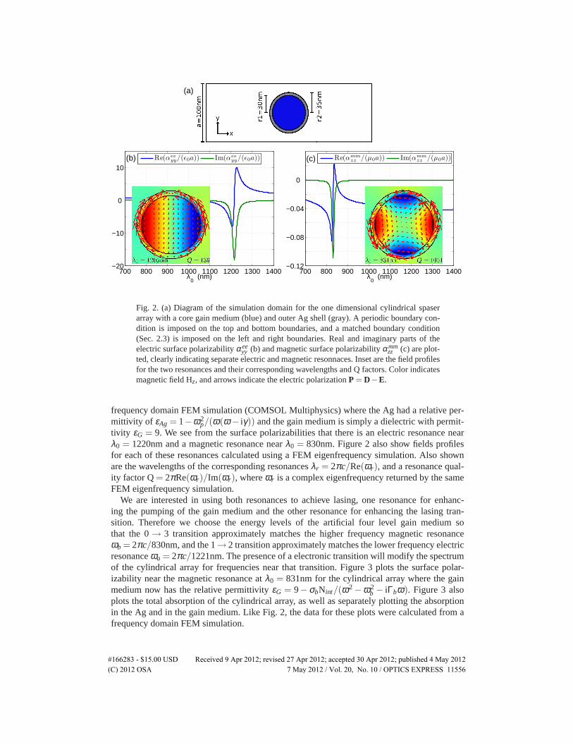
(a)

Fig. 2. (a) Diagram of the simulation domain for the one dimensional cylindrical spaserarraywith a core gain medium (blue) and outer Ag shell (gray). A periodic boundary con-dition is imposed on the top and bottom boundaries, and a matched boundary condition(Sec. 2.3) is imposed on the left and right boundaries. Real and imaginary parts of theelectric surface polarizabilityαee

yy (b) and magnetic surface polarizabilityαmmzz (c) are plot-

ted, clearly indicating separate electric and magnetic resonnaces. Inset are the field profilesfor the two resonances and their corresponding wavelengths and Q factors. Color indicatesmagnetic field Hz, and arrows indicate the electric polarizationP = D−E.

frequency domain FEM simulation (COMSOL Multiphysics) where the Ag had a relative per-mittivity of εAg = 1−ω2

p/(ω(ω − iγ)) and the gain medium is simply a dielectric with permit-tivity εG = 9. We see from the surface polarizabilities that there is an electric resonance nearλ0 = 1220nm and a magnetic resonance nearλ0 = 830nm. Figure 2 also show fields profilesfor each of these resonances calculated using a FEM eigenfrequency simulation. Also shownare the wavelengths of the corresponding resonancesλr = 2πc/Re(ωr), and a resonance qual-ity factor Q= 2πRe(ωr)/Im(ωr), whereωr is a complex eigenfrequency returned by the sameFEM eigenfrequency simulation.

We are interested in using both resonances to achieve lasing, one resonance for enhanc-ing the pumping of the gain medium and the other resonance for enhancing the lasing tran-sition. Therefore we choose the energy levels of the artificial four level gain medium sothat the 0→ 3 transition approximately matches the higher frequency magnetic resonanceωb = 2πc/830nm, and the 1→ 2 transition approximately matches the lower frequency electricresonanceωa = 2πc/1221nm. The presence of a electronic transition will modify the spectrumof the cylindrical array for frequencies near that transition. Figure 3 plots the surface polar-izability near the magnetic resonance atλ0 = 831nm for the cylindrical array where the gainmedium now has the relative permittivityεG = 9−σbNint/(ω2 −ω2

b − iΓbω). Figure 3 alsoplots the total absorption of the cylindrical array, as well as separately plotting the absorptionin the Ag and in the gain medium. Like Fig. 2, the data for these plots were calculated from afrequency domain FEM simulation.


780 800 820 840 860 880

−4

0

4

(a)

Re(αeeyy/(ǫ0a))

Im(αeeyy/(ǫ0a))

780 800 820 840 860 880−0.2

0

0.2

(b) Re(αmm

zz /(µ0a)) Im(αmmzz /(µ0a))

780 800 820 840 860 880 0

0.2

0.4

λ0 (nm)

(c) 1−|r|2−|t|2

Ag LossGain Loss

Fig. 3. (a) Electric surface polarizabilityαeeyy and (b) magnetic sufrace polarizabilityαmm

zz

for the cylindrical array with gain medium relative permittivity ofεG = 9−σNint/(ω2−ω2

b − iΓbω). (c) Total, absorption as well as absorption in Ag and absorption in the gainmedium. It is clear that the presence of the electronic transition in the gain medium stronglymodifies the spectrum of the cylindrical array.

We can see from Fig. 3 that the interaction of the electronic transition with the magnetic shaperesonance shown in Fig. 2(c) causes these resonances to hybridize. As a result the responseof the cylindrical array for frequencies near that transition is strongly modified. Instead of asingle magnetic resonance we see now see multiple resonances, both electric and magnetic.Examining the absorption plotted in Fig. 3(c) we see that the gain medium strongly absorbsat the magnetic resonance nearλ0 = 826nm. For our lasing simulations this will be the pumpfrequency. There is no way to know exactly what the lasing frequency will be without firstrunning the time domain lasing simulation, except to say that it will be approximately equalto the frequency of the 1→ 2 transitionωa. A good initial guess is to setω1 = ωa, but afterrunning the lasing simulation this can be adjusted to better match true lasing frequency. In whatfollows, we have usedω1 = 2πc/1219.3nm.

Figure 4 shows data from a time domain simulation of the cylindrical spaser array usingthe parameters defined above. The initial state of the simulation is prepared with a previoussimulation where the system is pumped with the fieldA2, with an intensity of 8W/mm2, whilethe incident probe field is set toA1 = 0. The pump beam is turned on slowly withA2 havingthe profile

A2 = Apuey12

[

1+er f

(

t −5τpu√2τpu

)]

, (22)


0 1 2 3 4

x 104

0

0.5

1

1.5

Inte

nsity

(W

/mm

2 )

t (2π/ω1)

(a)

0 1 2 3 4

x 104

7

7.5

8

8.5

9x 10

6

∫ Ωd

2x

(N2y

-N

1y)

t (2π/ω1)

(b)

6 6.5 7 7.5 80

0.02

0.04

0.06

0.08

0.1

0.12

0.14

Lasi

ng In

tens

ity (

W/m

m2 )

Pump Intensity (W/mm2)

(c)

slope = 0.145

threshold = 0.715W/mm2

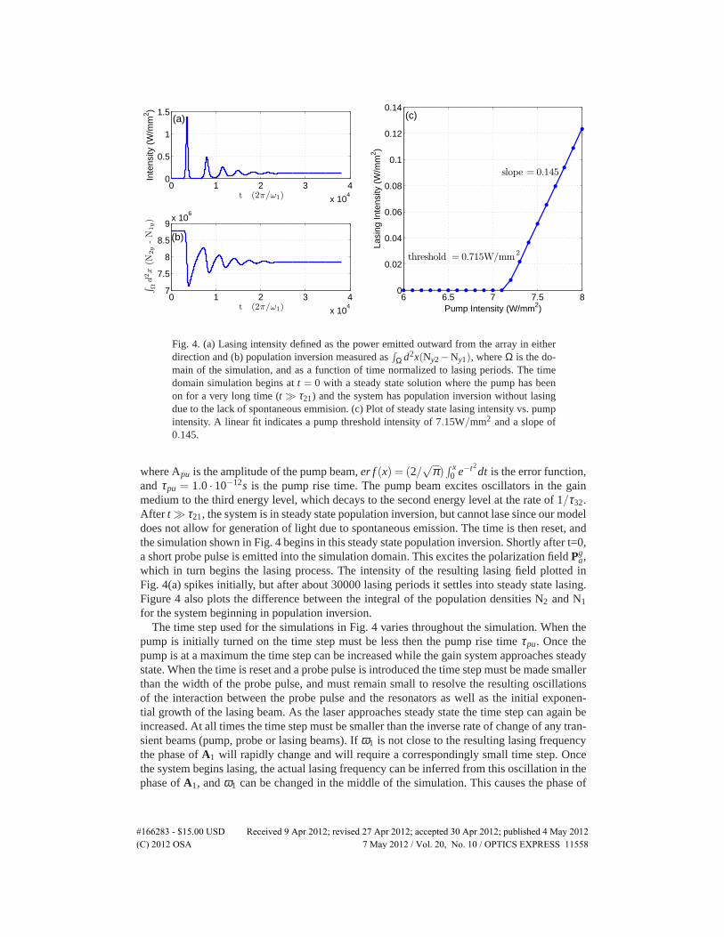
Fig. 4. (a) Lasing intensity defined as the power emitted outward from the array in eitherdirectionand (b) population inversion measured as

∫Ω d2x(Ny2−Ny1), whereΩ is the do-

main of the simulation, and as a function of time normalized to lasing periods. The timedomain simulation begins att = 0 with a steady state solution where the pump has beenon for a very long time (t ≫ τ21) and the system has population inversion without lasingdue to the lack of spontaneous emmision. (c) Plot of steady state lasing intensity vs. pumpintensity. A linear fit indicates a pump threshold intensity of 7.15W/mm2 and a slope of0.145.

where Apu is the amplitude of the pump beam,er f(x) = (2/√

π)∫ x

0 e−t2dt is the error function,andτpu = 1.0 · 10−12s is the pump rise time. The pump beam excites oscillators in the gainmedium to the third energy level, which decays to the second energy level at the rate of 1/τ32.After t ≫ τ21, the system is in steady state population inversion, but cannot lase since our modeldoes not allow for generation of light due to spontaneous emission. The time is then reset, andthe simulation shown in Fig. 4 begins in this steady state population inversion. Shortly after t=0,a short probe pulse is emitted into the simulation domain. This excites the polarization fieldPg

a,which in turn begins the lasing process. The intensity of the resulting lasing field plotted inFig. 4(a) spikes initially, but after about 30000 lasing periods it settles into steady state lasing.Figure 4 also plots the difference between the integral of the population densities N2 and N1

for the system beginning in population inversion.The time step used for the simulations in Fig. 4 varies throughout the simulation. When the

pump is initially turned on the time step must be less then the pump rise timeτpu. Once thepump is at a maximum the time step can be increased while the gain system approaches steadystate. When the time is reset and a probe pulse is introduced the time step must be made smallerthan the width of the probe pulse, and must remain small to resolve the resulting oscillationsof the interaction between the probe pulse and the resonators as well as the initial exponen-tial growth of the lasing beam. As the laser approaches steady state the time step can again beincreased. At all times the time step must be smaller than the inverse rate of change of any tran-sient beams (pump, probe or lasing beams). Ifω1 is not close to the resulting lasing frequencythe phase ofA1 will rapidly change and will require a correspondingly small time step. Oncethe system begins lasing, the actual lasing frequency can be inferred from this oscillation in thephase ofA1, andω1 can be changed in the middle of the simulation. This causes the phase of


1180 1200 1220 1240 1260

−60

−40

−20

0

20

40

60

λ0 (nm)

αee

yy/(ǫ

0a)

(a) 0 W/mm2

0.6 W/mm2

1 W/mm2

1180 1200 1220 1240 1260

−60

−40

−20

0

20

40

60

λ0 (nm)

αee

yy/(ǫ

0a)

(b) 1.8 W/mm2

2.4 W/mm2

3.4 W/mm2

Fig. 5. Real (solid lines) and imaginary (dashed lines) parts of the electric surface polar-izability αee

yy for the lasing electric resonance shown in Fig. 2 for various pump intensities(shown in legend). In Fig. 5(a) we see that at higher pump intensities the linewidth of theresonance narrows. In Fig. 5(b) we see that at even higher pump intensities the imaginarypart of the surface polarizability flips (indicating gain) and the linewidth of the resonancebegins to broaden.

A1 to slowly change allowing for a larger time step.There is a minimum pump intensity required for the light generated due to stimulated emis-

sion to overcome the internal losses in the cylindrical array. Figure 4(c) plots the steady statelasing intensity vs. the pump intensity. A linear fit to the lasing data points indicates a thresh-old pump intensity of 7.15W/mm2. This threshold intensity depends on a number of variables,including all of the parameters of the gain medium, as well as the cylinder plasmon resonancesused to enhance both the pump and lasing transition (Figs. 2 and 3). These resonances in turndepend on the geometry and material parameters of the cylindrical array.

While there is a minimum threshold intensity for the array to exhibit lasing, we can observeinteresting changes in the spectrum of the array at lower pump intensities. We saw by compar-ing Figs. 2 and 3 that the spectrum of the cylindrical array was changed by the presence of the0 → 3 transition. As we pump the array at increasing intensities we observe a similar changein the spectrum due to the 1→ 2 transition. Figure 5 plots the surface polarizability (Eq. (21))of the electric resonance for different pump intensities. These plots were created by pumpingthe cylindrical array with the fieldA2 for a long period of time (t ≫ τ21), and then injectinga Gaussian probe fieldA1 with a much weaker intensity. Applying a Fourier transform to theresulting time domain reflected and transmitted probe fields gives us the reflection and trans-mission amplitudes in the frequency domain, allowing us to calculate the surface polarizabilityaccording to Eq. (21).

From Fig. 5, we see that for increasing values of the pump intensity, the lineshape ofαeeyy

resembles a Lorentzian

αeeyy = αin f −

α0

ω2−ω2α − iγα ω

. (23)

We see in Fig. 5(a) that as we increase the pump intensity, it is as if the positive valued scattering


frequencyγα is made smaller, narrowing the lineshape. We see in Fig. 2(b) that at even higherpump intensities,γα continues to shrink, passing through zero, and the imaginary part ofαee

yychanges sign, indicating gain. As the pump intensity continues to increase,γα continues to growmore negative and the lineshape begins to broaden.

Even though we have gain at the pump intensities in Fig. 5(b), we still do not have lasingbecause the gain is not large enough to overcome radiative losses.

4. Conclusion

We have presented a finite element method simulation for a microphotonic lasing system. Wehave shown how to achieve a massive speedup in the simulation by separating the various fieldsinto fields that oscillate at the carrier frequenciesω1 or ω2, with slowly changing complex val-ued amplitudes. A demonstration of this simulation was provided with a two dimensional modelof a one dimensional cylindrical spaser array as an example. The threshold pump intensity forthis array was determined. Finally, we have shown how the linewidth of the lasing transitionchanges for various pump intensities.

Acknowledgments

Chris Fietz would like to acknowledge support from the IC Postdoctoral Research FellowshipProgram. Work at Ames Laboratory was supported by the Department of Energy (Basic En-ergy Science, Division of Materials Sciences and Engineering) under contract no. DE-ACD2-07CH11358.


Finite element simulation of microphotonic lasing...

Documents

Transcript of Finite element simulation of microphotonic lasing...