Finite element simulation of explosive welding

Mohammad Tabbataee, Jafar Mahmoudi

IST dep., HST School, MDH University, Box 883, SE 721 23, Västerås, Sweden mohammad.abbataee.ghomi@mdh.se jafar.ahmoudi@mdh.se

Abstract

Explosion welding or bonding is a solid-state welding process that is used for the metallurgical joining of dissimilar metals. The process uses the forces of controlled detonations to accelerate one metal plate into another creating an atomic bond. Explosion bonding can introduce thin, diffusion inhibiting interlayers such as tantalum and titanium, which allow conventional weld-up installation. In addition, explosive welding is considered a cold-welding process, which allows metals to be joined without losing their pre-bonded properties.

This paper describes work carried out to numerically analyze a two plate welding process using a finite element method (FEM) and the verification of the results using experimental data. The numerical simulations identify factors such as the level of strain induced in the plates and the direction of the shear stress at the collision zone, in the surface of flyer plates as indicators of bond strength. The phenomenon of jetting is computationally reproduced.

Keywords: Explosive welding; Ferrous metals and alloys; Wrought materials

1. Introduction

Explosive welding is a solid state welding process, which uses a controlled explosive detonation to force two metals together at high pressure. The resultant composite system is joined with a durable, metallurgical bond. Explosive welding under high velocity impact was probably first recognized by Garl in 1944. Explosive welding was first recognized as a possibility in 1957 in the United States when it was observed by Philipchuck that metal sheets being explosively formed occasionally stuck to the metal dies. Between that and now the process has been

developed fully with large applications in the manufacturing industry.

It has been found to be possible to weld together combinations of metals, which are impossible, by other means. This is a solid state joining process. When an explosive is detonated on the surface of a metal, a high pressure pulse is generated. This pulse propels the metal at a very high rate of speed. If this piece of metal collides at an angle with another piece of metal, welding may occur. For welding to occur, a jetting action is required at the collision interface. This jet is the product of the surfaces of the two pieces of metals colliding. This cleans the metals and allows to pure metallic surfaces to join under extremely high pressure. The metals do not commingle, they are atomically bonded. Due to this fact, any metal may be welded to any metal (i.e.- copper to steel; titanium to stainless). Typical impact pressures are millions of psi. Fig. 1 shows the explosive welding process.

Fig. 1. Explosion bonding process.

The process can be divided into three basic stages.

(i) The detonation of the explosive charge.

(ii) The deformation and acceleration of the flyer plate.

(iii) The collision between the plates.

Scheme of explosion welding with formation of cumulative jet presented here:

Fig 1. Welded join after sudden stop of explosion welding

where: U0, δ1 is velocity and thickness of general jet

Uc, δс is velocity and thickness of cumulative jet moving to the right (reverse)

Un, δn is velocity and thickness of jet moving to the left

To obtain a join at explosion welding it is necessary to follow to next conditions:

D < Co

where: Со sound velocity in welded materials

D is detonation velocity P ≥ Pкр

where: Ркр is a critical pressure in join

Р is a pressure in join γ < γкр

where: γ is an angle of collision , γкр is a critical angle of collision

According to the results of experiments about method of marks it is necessary to emphasize two points:

• Distance between the marks on the clad sheet doesn’t change along the full surface.

• Marks on the clad sheet coincide with their projections on the base sheet.

Fig. 2. Accepted scheme of explosion welding. Suggested scheme of explosion welding

where: V0 – plate velocity, γ – angle of collision, δL – next concerned element, а – zone of chemical reaction.

The absence of oblique collision at explosion welding doesn’t allow considering a process of join formation as a collision of straight and reverse liquid jet.

Zones singled out during join formation at explosion welding:

1- zone of contact point, 2- zone of ahead of contact point and 3- zone of join formation.

D – detonation velocity, Vв- velocity of shock-compressed gas, Vk – velocity of contact point.

Calculation of temperature into standoff:

Boltzmann’s equation

where R=8,31 (universal gas constant), µ=0,029 (molar mass of air), V– velocity of collision.

For the used conditions V = 2500 m/s (detonation velocity of mixture of porous ammonium nitrate with diesel oil 96:4) we obtain:

КT °≈⋅

⋅= 7270

31,83

029,025002

Calculation of stabilization length at explosion welding:

• h= 8 mm, D= 2500 m/s, V0= 400 m/s.

• Time of plate flight to collision is 20х10-6sec,

• Time of beginning of intense glowing of gas clot is 30-40х10-6sec.

Overall is 50-60х10-6sec.

• During all this time detonation passed 125-150 mm that conformed to stabilization site sizes observed in practice at manufacture of bimetal.

It is now generally accepted that jet formation at the collision point is an essential condition for welding. The jet if formed sweeps away the oxide layers on the surface of the metals leaving behind clean faces which are more likely to form a metallurgical bond by making it possible for the atoms of two materials to meet at interatomic distances when subjected to the explosively produced pressure waves. The pressure has to be sufficiently high and for a sufficient length of time to achieve inter-atomic bonds. The velocity of

µ

RTV

3=

R

VT

3

2µ=

the collision point, Vc (see Fig. 2) sets the time available for bonding. This high pressure also causes considerable local plastic deformation of the metals in the bond zone. As the bond is metallurgical in nature it is usually stronger than the weaker material. The quality of the bond depends on careful control of process parameters such as surface preparation, plate separation, detonation energy and detonation velocity Vd (see Fig. 2). While various welding mechanisms have been proposed for the explosive welding, they all almost agree that it occurs as a direct result of high velocity oblique collision. Experimental results indicate that there are certain critical values for both the collision and the geometrical parameters which have to be observed. These can be summarized as follows:

• Since a jet is required at the collision region, a collision angle β is critical. For a given metal, β is a function of the collision velocity [1]. It has been shown experimentally that the collision velocity Vc and the plate velocity Vp must be less than the velocity of sound in either metal. El-Sobky and Blazynski [2] used this to define the conditions necessary for the reflected stress waves not to interfere with the incident wave at the current collision point. It is also known that at supersonic velocities, the dynamic pressure is not held for a sufficiently long period to create physical conditions conducive to the adjustments of interatomic diffusion and of equilibrium within the collision region. While Wylie et al. [3] suggested that the velocity of sound may be exceeded by up to 25%; the subsonic collision appears to be more satisfactory. As Vc is related to Vd and β, it may be adjusted by introducing an initial angle of obliquity. The velocity of sound or more precisely, the velocity of stress wave propagation provides an upper limit for Vp and Vc.

• A minimum impact pressure must be exceeded (and hence a minimum Vp), in order that the impact energy should be sufficient to produce a weld. It has been suggested by Wylie et al. [3] that the impact energy required is related to the strain energy and the dynamic yield strength of the flyer material. An upper limit for the energy is also required to avoid excess heating and possibly melting by viscous dissipation and thus the formation of brittle layers. Obviously, such an upper limit should be sought in terms of the melting energy of the lower melting point of the weld combination.

• A sufficient stand-off distance has to be provided in order to flyer plate can accelerate to the required impact velocity.

Therefore, the critical parameters used to establish a weldability window are

• The critical collision angle for jet formation.

• The collision velocity, Vc.

• The kinetic energy and impact pressure in the collision region associated with the impact velocity, Vp.

Aspects of the welding process have been studied in detail by several investigators in the past. Attempts have been made, for example, to determine the velocity imparted to a plate by an explosive charge [4] and various empirical and semi-empirical equations have been suggested [5] and [6]. Attempts have also been made to find the minimum flyer plate velocity and impact angle required for bonding [5], [6], [7], [8] and [9]. Welding windows (of various parameters such as flyer plate velocity-impact angle and impact pressure-impact angle etc.) have been proposed by different authors [5], [6], [9] and [10].

The explosive welding trials with PETN and ANFO mixtures described in this paper were modeled using the ABAQUS/Explicit finite element [11].

ABAQUS/Explicit can utilize any constitutive equation that expresses the flow stress as a function of strain, strain-rate and temperature. They include amongst others, the Johnson–Cook [12] and Cowper–Symonds [13] constitutive equations for metals. In addition, ABAQUS can employ any equation of state that expresses pressure as a function of density and specific internal energy, for example, the Jones–Wilkins–Lee (JWL) equation of state [14] for high explosives, such as pentaerythritol tetranitrate (PETN), nitromethane etc. In this study, the analyses were performed with Johnson–Cook constitutive equations [12] (which relate the flow stress to strain, strain-rate and temperature). The JWL equation of state [14] was used for high explosives and the Williamsburg equation of state [15] coded into ABAQUS software was used for the ANFO mixture. The required parameters for the constitutive equations and equation of state used for plates and explosives respectively were extracted from the Autodyn material library [16] and [17].

The main aims of the work were to numerically simulate the process, to attempt to relate the process variables to the physical parameters and to establish how these can be used to predict whether or not bonding will occur. Part of this process included a program of welding tests using titanium and stainless steel cladding plates and carbon steel base plates. Most tests were done with the relatively slow ANFO explosive mixture. A few tests were conducted using PETN with a higher detonation velocity.

Few attempts to numerically model and simulate explosive welding have been reported in the literature. El-Sobky and Blazynski [2] studied the process using a liquid analogue. Their rationale was based on the similarity between hydrodynamic fluid behavior and material deformation close to the collision point in explosive welding. The strength of the material is small compared to the applied stress, therefore, for a short period of time the material behaves as if it were

a liquid. In metals there is a transition from inviscid flow to viscous flow, as stresses decrease solidification begins. In the latter case the strength of the material is negligible. This aspect of a liquid implies that in any liquid analogy mechanism for explosive welding only, the initial stages are important. Lazari et al. [18], [19], [20] and [21] used the finite element method to analyze the transient response of metal plates under explosive loading. Material non-linearity due to plasticity and strain-rate effects were considered. The problem was treated as normal transient loading of plane stress elements of rectangular shape. In this analysis, kinematically equivalent concentrated loads at the nodes represented the uniformly distributed explosive load. Oberg et al. [22] simulated explosive welding by means of a Lagrangian finite difference computer code, but only produced jetting. Akihisa [23] produced interface waves but no jetting. In addition, the author assumed that symmetric or asymmetric shear flow distribution was generated in the flyer and base plates and the modeling was performed based on this supposition. Akbari mousavi et al. [24], [25] and [26] simulated explosive welding using the Williamsburg equation of

state to model low detonation explosive such as ANFO mixture. They successfully reproduced the phenomena wave formations in explosive welding. Grigon et al. [27] simulated the straight interface and the phenomena of jetting using the Raven, an explicit multi-material Eulerian code [28]. However, no criteria for successful bonding have yet been demonstrated.

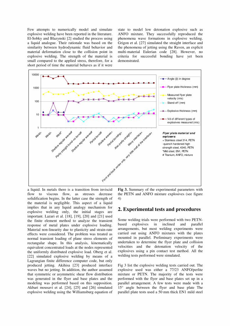
Fig 3. Summary of the experimental parameters with the PETN and ANFO mixture explosives (see figure 4)

2. Experimental tests and procedures

Some welding trials were performed with two PETN-based explosives in inclined and parallel arrangements, but most welding experiments were carried out using ANFO mixtures with the plates mounted in parallel. Preliminary experiments were undertaken to determine the flyer plate and collision velocities and the detonation velocity of the explosives using a pin contact test method. All the welding tests performed were simulated.

Fig 3 list the explosive welding tests carried out. The explosive used was either a 77/23 ANFO/perlite mixture or PETN. The majority of the tests were performed with the flyer and base plates set up in a parallel arrangement. A few tests were made with a 15° angle between the flyer and base plate The parallel plate tests used a 50 mm thick EN1 mild steel

1

10

100

1000

10000

Weld

+

Weld

+

Weld

*

Shallo

w re

gular

wav

es#

Partly

stra

ight

bon

d–no

bond

#

Shallo

w re

gular

wav

es#

Partia

l bond

#

Shallo

w w

aves

+

Partia

l bond

ing+

Also

partly

stra

ight+

Wavy

inte

rface

+

Front

and

back

vor

tex

only, v

ery little

melt a

t the

inte

rface

+

Angle (β) in degree

Flyer plate thickness (mm)

Measured f lyer plate

velocity (m/s)

Stand-off (mm)

Explosive thickness (mm)

Vd of different types of

explosives measured (m/s)

Flyer plate material and

explosers:

+ Stainless steel 314, PETN

-quench hardened high

strength steel, 4340, PETN

*Mild steel, EN1, PETN

# Titanium, ANFO, mixture

base plate (Metals Handbook, 2000; [29]) resting on sand. Tests were performed for several stand-off distances (from half to twice the flyer plate thickness) and for different thicknesses of explosive and flyer plate.

The ANFO detonation velocities as measured using a detonation velocity meter and the pin contact method [10], [30], [31], [32] and [33], varied between 1800 and 2600 m/s.

The test program was designed to determine the effect of changes in the operational parameters of the process (contact velocity, flyer plate velocity and dynamic angle) on the physical parameters such as effective stress, strain and contact pressure. Loading is due to detonation of the low explosive, which is in the form of 80 mm and 235 mm high powder mixtures covering the upper surface of the flyer plate for the different cases considered.

Most of the low explosives cannot generally be initiated by a detonator alone. A booster made of about 50–500 g of high explosive such as Composition C4, which can be initiated by a detonator, is used to start the detonation.

Following the tests two samples were cut from the central region of each welded plate, one sample parallel to the longitudinal axis of the plate, (i.e. in the direction of detonation), the other sample perpendicular to the direction of detonation. Each sample was polished and metallography of the region around the bond lines performed.

It was found that using an inclined plate arrangement with high explosive (PETN) the plates only partially bonded, whereas with the parallel arrangement and ANFO, bonding was almost 100% complete. In the case of the inclined plate set up bonding did not occur until approximately half way along the plate i.e. about 12 cm from the booster charge.

3. Modeling explosive welding

Numerical simulations of the experiments described above were carried out using ABAQUS version 6.4 [11]. The model has a novel approach to the problem in that no particular type of collision geometry or deformation pattern is pre-supposed. Starting with a given initial geometry, the gradual development of steady state collision geometry and the deformation pattern is calculated from the basic equation of motion. In this sense, the present computer model is better founded in fundamental physics than those previously reported. However, this does not imply that the present model is free from empirical elements. Empirical relationships and idealised behaviors (i.e. stress–strain models) constitute important parts of the

model. The Johnson–Cook equations [12] (see Appendix 1) and shock equations of state were used to simulate the behavior of the plates. These equations describe the behavior of materials subjected to large strains, high strain-rates and high temperatures resulting from intensive impulsive loading due to high velocity-impact and explosive detonation. The material constants were determined from experimental tests. The flyer and base plates were modeled using Arbitrary Eulerian Lagrangian formulation for both components. The code requires the user to specify a mode for tensile failure with the Johnson–Cook plasticity model from a number of options. For this work the tensile failure was set to a value of 5 GPa for the stainless steel and 4 GPa for the titanium plates. The Mohr–Coulomb model [34], was used for the sand on which the plates rested and the JWL [14] (see Appendix 2) and Williamsburg EoS [24] for the explosive. In the ABAQUS code, energy and momentum transfer was through contact surfaces between the base of the explosive and the upper surface of the flyer plate and between the lower surface of the flyer plate and the upper surface of the base plate. The base of the sand anvil was fixed in a direction perpendicular to its surface. The lower surface of the explosive and the upper surface of the flyer plate were represented by independent nodes and their interactions specified by appropriate contact algorithms.

The loading is due to the detonation of the PETN high explosive (9 and 75 mm sheet covering the upper surface of the flyer plate) and the various thicknesses of ANFO mixture low explosive (80, 107, 135 and 235 mm).

It was found that the size of mesh was also important in visualizing the large velocity vectors which indicated jetting at the interface. In the areas close to the collision zones where the jet forms, mesh size of about 0.02 mm were used, in other areas the meshes were made an order of magnitude larger. Friction was also included in the modeling with a value of about 0.3 chosen as optimum for the coefficient of friction [30]. The initial model assumed no bonding criteria. Later some criteria (see later section), were inserted into the model. Comprehensive descriptions of the modeling can be found in [30] and [31].

The data obtained from the simulations were validated by the explosive welding trials as well as impact welding tests [24] and [25].

3.1. Williamsburg equation of state applied to

ANFO mixtures

Low detonation velocity explosives cannot be modeled with the widely used Jones–Wilkins–Lee (JWL) EoS [14] as the reaction zone at the detonation

front is thick compared with high explosives. This means the energy and momentum in the von-Neumann spike cannot be neglected [35] and [36] and the Chapman–Jouguet [17] pressure is more than that calculated using the JWL EoS, and a reactive model is required [30]. The JWL is empirical and assumes the Gruneisen gamma coefficient is constant, and is not a complete EoS, so that temperature and entropy cannot be calculated without a crude assumption, for example that heat capacity is constant, which is not true. There is always a large increase of specific entropy on going from explosive to products. The JWL EoS can only be employed assuming thermal isolation, as the temperature is not defined. Consequently, a new approach using the Williamsburg EoS [35] was adopted with all the relevant parameters being determined from experimental measurements and thermodynamic analyses.

The Williamsburg equation of state [24] is a semi-empirical EoS which relates the internal energy U to the specific volume V and the specific entropy S. Pressure is also calculated by means of U, V and S. The small number of parameters required are found by fitting to the principal adiabats calculated using a detonation code SIRIUS [37]. SIRIUS incorporates the Theostar [38] and Murnaghan [39] EoS for detonation products and silica, respectively, which are based on statistical mechanics and intermolecular potentials. The reference state in the Williamsburg equation of state is the detonation state, which is assumed to be ideal. i.e. satisfying the assumptions of the Chapman–Jouguet theory [14]. The main assumption is that the reaction zone, in which the explosive decomposes to form stable molecular products in chemical and phase equilibrium, is extremely thin and flat. The Williamsburg equation of state energy equation of order N in terms of reduced variables v is

kk

k

ref

N

kk

kUSVU

γα

υ β

υσβ

γ ∏=

+

+=

−

1

)1

1(),(

1

(1)

Where

refV

V=υ

,

−=

Rn

SSEXP

ref

ref )(σ

and R is the gas constant. The equations involve 4N + 4 basic parameters (the k, βk, γk, δk, and Uref, Vref, Sref, nref). The reference values of Uref, Vref, Sref and nref are the Chapman–Jouguet (CJ) values. Further information on the Williamsburg equation of state, including how to extract the quantities required by the simulation software, such as

pressure, and Gruneisen gamma can be found elsewhere [35] and [24].

4. Finite element modeling

4.1. Description of the code

The finite difference and finite element communities have used Eulerian methods for over 30 years to analyze problem with explosive loading, but until comparatively recently, they were too computationally demanding and inaccurate to be attractive for solving problems in solid mechanics. The strengths and weaknesses of the Eulerian formulation are summarized here in a brief description of the computational methods used in Raven, an explicit, multi-material Eulerian program developed by David Benson [28]. The review by Benson [29] discusses the algorithms in greater detail. Benson and coworkers [30] successfully used Raven in the computation of explosive compaction and shock synthesis.

Operator splitting replaces a differential equation with a set of equations that are solved sequentially. To illustrate its application in a multi-material Eulerian code, consider Eq. (2), a simple transport equation, where φ is a solution variable, u is the velocity, and Φ is a source term.

φϕϕ

=∇+∂

∂.u

t

r

(2)

This equation is split into two equations,

φϕ

=∂

∂

t (3)

0. =∇+∂

∂ϕ

ϕu

t

r

(4)

Where (3) and (4) are referred to as the Lagrangian and Eulerian steps, respectively. The Lagrangian step uses the central difference algorithm to advance the solution in time in the same manner as a standard explicit Lagrangian finite element formulation.

The Eulerian step is equivalent to a projection of the solution from one mesh onto another, and a perfect projection should be completely conservative. Most transport algorithms are conservative by construction: a flux added to one element is subtracted from its neighbor. Van Leer [31] developed the MUSCL transport algorithm used in the current calculation. The transport volumes are geometrical calculations defined by the mesh motion and they are independent

of the transport kernel. The 1D algorithm is extended to 2D by performing sweeps along one mesh direction, then another sweep in the other direction.

4.2. Material models

The Johnson–Cook constitutive model [32] was used for the 6061 T0 aluminum alloy. The advantage of this equation is that the five parameters can easily be extracted from mechanical tests. The Johnson–Cook equation is

−

−−++= m

rm

rn

TT

TTCB )(1)ln1)((

00 ε

εεσσ

(5)

The five parameters are σ0, B, C, n, and m. Tr is a reference temperature (at which σ0 is measured) and

is a reference strain rate (often equal to 1). The first term gives the stress as function of strain with

and T*=0. The second and the third terms represent, respectively, the strain rate and the temperature effects. The values of the parameters were derived from quasistatic and dynamic mechanical tests carried out on the 6061 T0 aluminum alloy. The dynamic tests were conducted in a split Hopkinson bar at varying temperatures. The results of the mechanical tests are presented in Fig. 11. The JC parameters obtained from the experiments are

σ0=60 MPa, n=0.3,B=500 MPa, m=1.C=0.02,

For the explosive, the Jones–Wilkins–Lee [33] equation of state was chosen to represent the expansion of the explosive products. The JWL equation of state defines pressure as function of relative volume (inverse of density), V, and internal energy per initial volume, E, as

V

Ee

VRBe

VRAP

VRVR ωωω+−+−= 21 )1()1(

21 (6)

Where P is the pressure, V is the relative volume, E is the internal energy, ω is the Gruneisen parameter, and A, B, R1 and R2 are constants which satisfy the mass, momentum, and energy conservation equations.

5. Results of model

The simulations showing 3D maps and profiles of a number of physical parameters, such as contact pressure, shear stress, normal stress, plastic strain, effective strain, strain rate, internal energy, kinetic energy, temperature and velocity of the flyer plate at

the point of contact and the angle of contact. Plots of mesh and material boundaries, and quantities as a function of time and distance for given co-ordinate were also available.

For the sake of clarity, only a representative sample of the simulations of the experimental tests is presented here. The results are presented in the following order (they are also listed in Fig 6).

The overall movement of the flyer plate; Vertical and horizontal velocities of flyer and base plates; Maximum pressure (P); Maximum shear stresses (S12); Maximum strains; The maximum base plate velocity (assuming the base plate moves after impact); The maximum impact angle. These variables are discussed later and finally the collision velocities calculated by dividing the length of the material by the total timing of the simulation process.

Comparisons of these results with experiments are presented in a later section.

Models for tests 1, 3 and 10 are shown in Fig. 7, Fig. 8

and Fig. 9, respectively. The explosive thickness is divided into 60, 350 and 600 elements for tests 1, 3 and 10, respectively, and is shown in red1. The flyer plate is modeled using 50, 90, and 45 thickness elements for tests 1, 3 and 10 respectively, and is shown in blue. The base plate is shown in cyan and has 200 elements through its thickness with appropriate grading. The sand anvil is modeled using 400 elements through its thickness with appropriate grading and is shown in green. Tests 4 and 5 were also inclined geometry arrangements. In all cases, the lowest mesh size was used for in regions near the

0 0.1 0.2 0.3 0.4 0.5 0.6 0.7 0.8 0.9 1-400

-350

-300

-250

-200

-150

-100

-50

0

50

100

Distance of plates [m]

Velo

city [

m/s

]

Flyer plate

Base plate

contact surfaces, further away the meshes were made larger.

5.2. Validating the numerical results

The impact velocities of the plate predicted by computational simulations agree with experiments (see Fig 6). The collision velocities calculated by dividing the length of the material by the total timing of the simulation process was in agreement with experiments. Due to the geometry of the process at the collision point, the dynamic angle defined as sin B=Vp/Vc [40] is in agreements wit the data obtained from the simulations. Fig 6 also shows maximum pressure (P), maximum shear stresses (S12), the maximum base plate velocity (assuming the base plate moves after impact) and the maximum impact angle. These variables are discussed later.

For PETN and ANFO/mixtures the pressure at the detonation front is equal to the Chapman–Jouguet (CJ) value [15]. This confirms that the coding was

performed correctly and the constitutive equations and the equations of state used to model the behavior of plates and explosive were correctly chosen. The predicted velocities were also in reasonable agreement with experiment. This leads to the assumption that the predicted impact angle should also be similar to that occurring in practice.

Based on this assumption, the numerical analysis was used to investigate the “local mechanism” at the collision point in order to identify the internal (physical) processes linked to the external (operational) parameters.

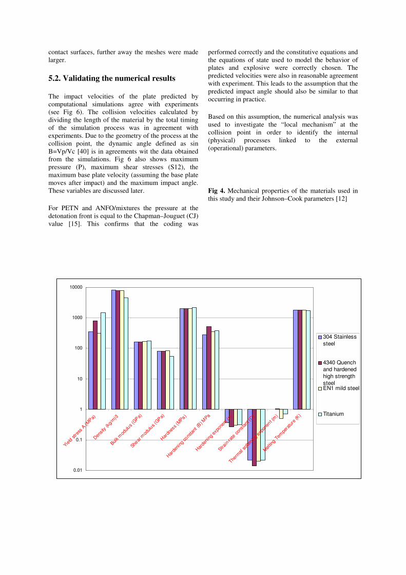
Fig 4. Mechanical properties of the materials used in this study and their Johnson–Cook parameters [12]

0.01

0.1

1

10

100

1000

10000

Yield s

tress

A (M

Pa)

Den

sity

(kg/

m)3

Bulk m

odulus

(GPa)

Shear

mod

ulus

(GPa)

Har

dnes

s (M

Pa)

Har

deni

ng cons

tant

(B) M

Pa

Har

deni

ng e

xpon

ent (

n)

Strain

-rate

con

stan

t (C)

Therm

al s

ofte

ning

expo

nent (

m)

Mel

ting T

empe

ratu

re (K

)

304 Stainless

steel

4340 Quench

and hardened

high strength

steelEN1 mild steel

Titanium

Fig 5. JWL parameters of the explosive used [14], CJ, Chapman–Jouguet [15] and [17]

Fig 6. Variables results obtained from the analysis

For pure ANFO the velocity of sound is 3667 m/s and the adiabatic gamma is 2.881.

0.1

1

10

100

1000

10000

Det

onatio

n ve

locit

y (m

/s)

Den

sity

(kg/

m3)

CJ

ener

gy (M

J/m

3)

CJ

pres

sure

(GPa)

C1

(GPa)

C2

(GPa) r1 r2

PETN

PETN

Pure ANFO

ANFO mixture

0.01

0.1

1

10

100

1000

10000

0 5 10 15 20 25

Measured f lyer plate

velocity (m/s)

Predicted f lyer plate

velocity (m/s)

Explosive ratio (R)

Predicted maximum impact

angle (°)

Predicted collision velocity

(m/s)

Predicted maximum

pressure (GPa)

Predicted maximum shear

stress (GPa)

Predicted maximum plastic

strain

Terminal velocity (Gurney)

(m/s)

Fig. 7. Inclined geometry arrangement and meshed form.

Fig.8. Parallel geometry arrangement.

Fig. 9. Parallel geometry arrangement.

5.3. Vertical and horizontal velocities of

flyer and base plates

The flyer plate was accelerated initially by a shock wave, resulting from the detonation pressure, and then by the expanding gaseous products of detonation. If the stand-off distance between flyer and base plates was sufficiently large, the flyer plate eventually attained a terminal velocity. The vertical velocity profile for the flyer obtained from the ABAQUS analyses are shown in red in Fig. 9 for test 3. Fig. 9 shows that the velocity increases from zero to its highest at the collision point and then the velocity reaches zero. The predicted vertical velocities compared well with those measured by pin contact tests (see Fig 6). For the tests carried out with the PETN explosive, the terminal velocities were reached. Therefore the vertical velocities can also be compared with the Gurney velocities [4]

Fig. 10. Vertical velocity of flyer and base plate at 0.6 m from the edge of the plates.

, where VT is flyer plate terminal velocity, Vd is detonation velocity and R=mp/mc is the charge to plate mass ratio, mp is plate mass per unit area and me is the charge mass per unit area and k is the polytropic constant of explosive. The polytropic constant is 2.3 for PETN explosive and 2 for ANFO mixture [30].

The highest values were generated in parallel plate geometries. The vertical component of the flyer plate also agreed with that determined using the Gurney velocity, see Fig 6. The Gurney equation [4] calculates the velocity perpendicular to the surface; therefore its value was compared with the value of vertical velocity obtained from this analysis (shown in Fig. 9). The profiles of the vertical velocity of the base plate shows that the contact surface exhibits the condition of Helmholtz discontinuity [41] i.e. the vertical velocity is positive ahead and negative behind the collision point, see Fig. 9. The vertical velocity of the base plate in green, if it assumed it moved when impacted, increases to its highest negative behind the collision point, return to zero at the collision zone and increases to its highest positive ahead of the collision zone.

The velocity of the flyer plate increases as the plate moves down towards the base plate. The velocity of the base plate also increases on impact. As these two velocities are of opposite sign, it is clear that at some point on the interface, the velocities of the flyer and base plates will be equal. These velocities are

compared with the minimum velocities required for bonding in Fig 8 later in this paper.

5.4. Contact pressure and pressure

distributions.

An example of the variation of contact pressure, i.e. the pressure normal to the surface is shown in Fig. 11 (test 2) for a point 0.6 m from the edge of the plate. The contact pressures are about 107 Pa. In the inclined geometries, the contact pressure profile spreads further ahead of the collision point than in the parallel geometries.

Fig. 11. Contact pressure (normal to the contact surface) for test 2.

The pressure applied on the surface of the both flyer and base plates (at one instant in time) for test 3 is shown in Fig. 12. The pressure profiles for the flyer plate are shown in red and for base plates in green.

Fig. 11. Pressure profiles of flyer and base plates (test 3) at one instant in time.

In all cases, whether the collision point moves with subsonic, sonic or supersonic velocity, the pressure

generated immediately at collision must be sufficient to exceed the dynamic elastic limit of the material to ensure deformation of the metal surface into a jet. The typical predicted pressure distributions around the point of contact are shown in Fig. 13 and Fig. 14 for the tests 1 and 2, respectively. The spread of the pressure on the surface depends on the angle of impact and the magnitude of the pressure. It can be seen that the pressure distribution depended on the angle between the flyer and base plate. For the inclined geometry the pressure distribution was spread furthest in front of the collision point and its maximum level was about one third of that seen in the parallel arrangement.

Fig. 13. Inclined arrangements – pressure contour for test 1.

Fig. 14. Parallel arrangements – pressure contour for test 2.

The highest pressure predicted was at the collision point and of the order of 109 Pa, see Fig 6. An interesting feature of the inclined plate simulation is the presence of a small ‘hump’ on the surface of the base plates ahead the point of contact (see Fig. 13). This hump only appeared in the simulations of the experiments in which the plates bonded. It is shown

that the pressure distributions are more localized in the inclined geometry than the parallel geometry due to the increased in the angle between the flyer and base plates. In the case of the PETN explosive with very high velocity of detonation (7450 m/s), the pressure wave made a 30° angle with the horizontal surface in the base plate (see Fig. 14). This is because the speed of detonation is higher than the speed of the sound in the material. In the parallel arrangement with the PETN explosive, the shock is attached (the contact periphery moves supersonically i.e. no jet) as predicted in [42], [43] and [44]. In the inclined set-up the shock produced is detached due to the increased angle reducing the velocity of deformation. Cowan et al. noted that if the shock was attached, no bonding occurred because the pressure did not spread ahead of the collision point to produce surface deformation and jetting. No weld was obtained in this arrangement. For test 2 (a parallel arrangement), with the detonation velocity lower than the speed of sound, the contact periphery moved subsonically (i.e. creating a jet) and welding occurred. The simulation results confirmed Cowan’s prediction, Holtzman [42]. The results also show that if only one plate contributed to the jet, the pressure maximum was closer to the surface of the other plate. This may be due to loss of material from the surface of the jet producing plate.

Fig 15: temperature distribution in explosion instace

5.5. Dynamic angle profiles

The dynamic angle is one of the influential parameters in explosive welding. The dynamic angles predicted in the simulations are shown Fig 6. This shows the sum of the angles between the flyer and the x-axis and between the base plate and x-axis. The dynamic angles for tests 1–3 were 17.5°, 2.3° and 5.25°, respectively. The dynamic angle obtained for the inclined geometry arrangement (17.5°) was greater than its initial angle (15°).

5.6. Strain-rate

Mechanical strain-rates of the order of 103 s−1 were obtained in these analyses. This is much lower than the strain-rate calculated by [45]. However, his data was obtained using hydrodynamic theory and assuming the shear strength of the materials could be neglected. Hydrodynamic theories give a very high value of pressure and thereby a very high strain-rate. It is shown in [24] that the sizes of the interface waves produced using the hydrodynamic treatment were greater than the experimental results by 30%. Using the strength models to describe the behavior of metals a reasonable agreement was found between the wave sizes obtained from the simulation and the experimental results.

6. Discussion

The impact velocity of the plate predicted by computational modeling agrees very well with experiment. The collision velocity in the simulation was obtained by dividing the length of the material by the total timing of the simulation process was also in agreement with experiments. With the same impact angle as that used in the experiments the computational model was used to investigate the “local” mechanism at the collision point, to assist the identification of the internal processes and to link them to external parameters.

7. Conclusions

The present study has made it possible to model the main features of the explosive welding process. Relationships between operational conditions and physical parameters, such as local stresses, strains and particle velocities which determine the success or failure of the weld were identified.

In general, the choice of contact algorithm, kinetic or penalty (see ABAQUS manual for details) made little difference to the results. Bonding is dependent on the level of induced plastic strain in the two materials exceeding a threshold level. Shear stresses induced in the two plates were not always of the same sign. In the case of simulations of the bonded plates the shear stresses were of opposite sign but had the same sign for non-welded plates. The predicted impact velocities were in very good agreement with experiment and calculations made using the Gurney equation.

According to this investigation, the influential physical parameters affecting explosive bonding can be defined as effective strain, shear stress. The formation of a hump in the collision zone was found in the cases where bonding occurred. The occurrence of jet can be shown by simulations. The simulations confirm some of the previous results for the explosive welding process.

References

[1] J.M. Walsh, R.G. Shreffler and F.J. Willig, Limiting conditions for jet formation in high velocity collision, J Appl Phys 24 (3) (1953), pp. 349–359.

[2] El-Sobky H, Blazynski TZ. Experimental investigation of the mechanics of explosive welding by means of a liquid analogue. In: Proc 5th int conf on high energy rate fab, Denver, Colorado, vol. 4(5); 1975. p. 1–21.

[3] Wylie HK, Williams PEG, Crossland B. Further experimental investigation of explosive welding parameters. In: Proc 2nd int conf cent high energy fab, vol. 1(3); 1971. p. 1–43.

[4] Gurney RW. The initial velocities of fragments from bombs, shells and granades. Ballistic Research Laboratory 1947; Report No. 405. Aberdeen Proving Ground, Maryland.

[5] Lazari GL. Explosive Welding of multi-Laminate Composites. PhD thesis UMIST; 1986 [Chapter 3].

[6] Kowalewskij V, Belajew W, Smirnow G. Application of explosive welding in manufacturing of composite materials, Belorussisches Polythechnisches Institute, Minsk, UDSSR, Explosionsschweiben von Verbunmaterialien, vol. 70(2); 1979. p. 67–70.

[7] Wittman RH. Use of explosive energy in manufacturing metallic materials of new properties. In: 2nd int symp, 1973; Marianski, Lazne, Czechoslovakia.

[8] Crossland B, McKee FA, Szecket A. An experimental investigation of explosive welding parameters. In: Proc 6th air conf, Boulder; 1977. p. 805–13.

[9] Loyer A, Talerman M, Hay DR. Explosive welding, the weldability window for dissimilar metals and alloys. In: 3rd int symp use of expl ener in man met mat new prop; 1976. p. 43.

[10] Szecket A. An experimental study of the explosive welding window. PhD thesis, Queen’s University of Belfast; 1979.

[11] Hibbit HD, Karlson BI, Sorenson D. ABAQUS User Theory Man version 6.4. HKS Inc., Rhode Island USA; 2004.

[12] Johnson RG, Cook WH. A constitutive model and data for metals subjected to large strains, high

strain-rates and high temperature. In: Proc 7th int symp ball the hague the Netherlands; 1983. p. 541–47.

[13] P.S. Symonds In: N.J. Muffington, Editor, Visco-elastic behavior in response of structures to dynamic loading, ASME, New York (1987), pp. 106–125.

[14] Lee EH, Hornig HC, Kury JW. Adiabatic expansion of high explosive detonation products. 1968; Rep UCRL-50422, Lawrence Livermore National Laboratory Livermore CA USA.

[15] Byers Brown W, Braithwaite M. Williamsburg equation of state for detonation product fluid. Shock Comp Cond Matt, Colorado; 1993.

[16] Autodyn manual, Century Dynamics. 2003; Ver. 2.6.

[17] M.A. Cook, The science of high explosives, Reinhold Publishing Corporation, New York (1958).

[18] Lazari GL, Al-Hassani STS. Solid mechanics approach explosive welding composite. In: Proc 8th int conf on high energy rate fabrication, San Antonio; 1984.

[19] S.T.S. Al-Hassani, S.A. Salem and G.L. Lazari, Explosive welding of flat plates in free flight, Int J Imp Eng 1 (2) (1984), pp. 85–101.

[20] Al-Hassani STS, Salem SAL Interfacial wave generation in explosive welding of laminates. In: Mayers A, Murr L, editors. Shock waves and high strain phenomena in metals; 1981 [Chapter 57].

[21] S.T.S. Al-Hassani and G.L. Lazari, Explosive welding of tapering plates. In: L.E. Murr, K.P. Staudhammer and M.A. Meyers, Editors, Metallurgical applications of shock-wave and high strain-rate phenomena, Marcell Deckker Inc., NY, Basel (1986) [Chapter 53].

[22] A. Oberg, J.A. Schweitz and H. Olfsson, Computer modeling of the explosive welding process, Proc int conf on high energy rate fabrication (1984), pp. 75–84. [23] A.B.E. Akihisa, Numerical study of the mechanism of a wavy interface generation in explosive welding, JSME Int J Series B 40 (3) (1997), pp. 395–401.

[24] A.A. Akbari Mousavi, S.T.S. Al-Hassani, S.J. Burley and W. Byers Brown, Simulation of explosive welding with ANFO mixture, J Prop Exp Pyro 29 (3) (2004), pp. 188–196.

[25] A.A. Akbari Mousavi and S.T.S. Al-Hassani, Simulation of explosive welding using Williamsburg

equations of state to model low detonation velocity explosive, Int J Imp Eng 31 (2005), pp. 719–734.

[26] Akbari Mousavi AA, Al-Hassani STS. Simulation of wave and jet formation in explosive/impact welding. In: Proc. 7th Biennial ASME Conf, The ASME conf eng sys des anal, Manchester; 9–22 July 2004.

[28] Benson, DG. Raven user’s man, Ver; 2001.

[29] Metals Handbook, ASM, The materials information society.

[30] Akbari Mousavi AA. The mechanics of explosive welding. University of Manchester Institute of Science and Technology UMIST PhD thesis; 2001.

[31] Al-Hassani STS. Numerical and experimental investigation of explosive bonding process, variables and their influence on bond strength. EPSRC Grant GR/M10106/01, Final Report, University of Manchester Institute of Science and Technology UMIST; 2001.

[32] Al-Hassani STS, Akbari Mousavi AA. The experimental investigation of explosive welding. In: Proc. 6th SMEIR conference, Amir Kabir University of Technology, Tehran, Iran; 2003.

[33] Al-Hassani STS, Akbari Mousavi AA. Recent development on the response of materials and structures to impact and explosion (the case for explosive and impact welding). In: Proc 4th int conf eng sci, Gilan University Gilan, Iran; 2000.

[34] Hancock S. Soil and rock strength models. Pieces 2DELK Application Note, vol. 78; 1979. p. 14.

[35] W. Byers Brown, Analytical representation of the adiabatic equation for detonation products based on statistical mechanics and intermolecular forces, Philos Trans Ry Soc A 339 (1992), pp. 345–353.

[36] W.C. Davis, The detonation of explosives, Sci Am 256 (5) (1987), pp. 98–106.

[37] Byers Brown W. SIRIUS code. Williamsburg equation of state for fluids at very high density. ICI plc Explosive Group Technical Center, Ardeer; 1994.

[38] T.V. Horton, Analytical representation of high density fluid equations of state based on statistical mechanics. In: S.C. Schmidt and N.C. Holmes, Editors, Shock waves in condensed matter, Elsevier BV, Amsterdam (1987).

[39] Byers Brown W, Behain A. Review of equations of state of fluids valid to high density. HSE; 1991.

[40] B. Crossland, Explosive welding of metals and its application, Oxford University Press, New York (1882).

[41] J.M. Hunt, Wave formation in explosive welding, Phil Mag 17 (148) (1968), p. 669. [42] A.H. Holtzman and G.R. Cowan, Flow configuration in colliding plates: explosive bonding, J App Phy 34 (4) (1963), pp. 928–939 Part 1.

[43] A.H. Holtzman and G.R. Cowan, Bonding of metals with explosive, Weld Res Coun Bull 104 (1965), pp. 1–21.

[44] G.R. Cowan, O.R. Bergman and A.H. Holtzman, Mechanics of bond wave formation in explosive cladding of metals, Met Tran 2 (1971), p. 3145.

[45] Robinson JL. A fluid model of impact welding. In: Proc 5th int conf high ener rate form phil mag, vol. 31(1); 1975. p. 587.