Finite element modelling of earth pressure on abutment ...
56
Publications of the FTIA 32/2020 FINITE ELEMENT MODELLING OF EARTH PRESSURE ON ABUTMENT PILES OF INTEGRAL BRIDGES
Transcript of Finite element modelling of earth pressure on abutment ...

Publications of the FTIA
32/2020
FINITE ELEMENT MODELLING OF
EARTH PRESSURE ON ABUTMENT
PILES OF INTEGRAL BRIDGES


Finite element modelling of earth pressure on
abutment piles of integral bridges
Publications of the FTIA 32/2020
Finnish Transport Infrastructure Agency
Helsinki 2020

Online publications pdf (www.vayla.fi)
ISSN 2490-0745
ISBN 978-952-317-785-7
Finnish Transport Infrastructure Agency
P.O.Box 33
FIN-00521 HELSINKI, Finland
Tel. +358 (0)295 34 3000

Publications of the FTIA 32/2020 3
Foreword
This study was prepared by Ramboll Finland Ltd on behalf of Finnish Transport
Infrastructure Agency (FTIA). The objective of the study was modelling the earth
pressure on abutment piles of integral bridges with finite element analyses. The
results were converted to a simplified analytical calculation model to be used in
structural design of integral bridges.
The study was carried out by Marco D'Ignazio, PhD, Ville Lehtonen, PhD and Lauri
P. Savolainen, MSc, from Ramboll Finland Ltd. The study was supervised by Veli-
Matti Uotinen and Panu Tolla from FTIA.
Helsinki, December 2020
Finnish Transport Infrastructure Agency

Publications of the FTIA 32/2020 4
Contents
1 INTRODUCTION ........................................................................................................... 5
2 ANALYTICAL SOLUTION FOR EARTH PRESSURE ON ABUTMENT PILES OF
INTEGRAL BRIDGES .................................................................................................... 7
3 DEFINITION OF PROBLEM FRAMEWORK ............................................................... 8 3.1 Geometries .................................................................................................................. 8 3.2 Loads ............................................................................................................................. 9 3.3 Calculation matrix...................................................................................................... 9
4 FINITE ELEMENT MODEL ......................................................................................... 11 4.1 Geometry and mesh ................................................................................................. 11 4.2 Load configurations .................................................................................................12 4.3 Construction phases and calculation steps ...................................................... 14 4.4 Earth pressure modelling ....................................................................................... 15
5 MATERIAL MODELS AND PARAMETERS ............................................................... 17 5.1.1 Hardening Soil model ................................................................................. 17 5.1.2 Mohr-Coulomb model ............................................................................... 20 5.1.3 Linear Elastic parameters for piles ........................................................ 20
6 RESULTS ..................................................................................................................... 22 6.1 Model performance and behaviour ..................................................................... 22 6.2 Mesh sensitivity check ........................................................................................... 24 6.3 Effect of traffic load configuration ...................................................................... 24 6.4 Earth pressure: FEM vs analytical solution ....................................................... 25 6.5 Earth pressure on active vs passive side ........................................................... 32 6.6 Pile displacements................................................................................................... 34 6.7 Earth pressure distribution ................................................................................... 39
7 IMPROVEMENT OF ANALYTICAL SOLUTIONS FOR EARTH PRESSURE .......... 45
8 DISCUSSION .............................................................................................................. 48 8.1 Using the results of this study when modelling a pile slab ......................... 48 8.2 Limitations of this study ....................................................................................... 48
9 SUMMARY, CONCLUSIONS AND RECOMMENDATIONS FOR FUTURE
RESEARCH WORK...................................................................................................... 50 9.1 Summary and conclusions..................................................................................... 50 9.2 Recommendations for future research work .................................................... 51
REFERENCES......................................................................................................................... 53
Publications of the FTIA 32/2020 5
1 Introduction
Väylävirasto (hereinafter referred to as Väylä or the Client) has asked Ramboll
Finland Oy (Ramboll) to perform a study aiming to model the earth pressure on
abutment piles of integral bridges. Bridge abutments are often founded on piles,
especially in presence of difficult soil conditions.
Structural design of piles is strongly affected by the earth pressure acting along
the piles during the construction of the road embankment and superstructure
and under the action of traffic loads. The mobilized earth pressure is commonly
determined analytically based on the simplified solution in Sillan geotekniset
suunnitteluperusteet (“Geotechnical design criteria for bridges”, Tiehallinto
2007). This solution accounts for the weight of the soil above the pile and the
applied traffic load. The resulting earth pressure increment is calculated based
on the earth pressure coefficient at rest (Ko) of the embankment/superstructure
material and assuming a 2:1 stress distribution with depth.
Soil conditions and drainage during loading are expected to have an impact on
the actual earth pressure. These aspects cannot be captured by the simplified
analytical solution. Therefore, this study aims to compare the analytical
approach to 3D Finite Element (FE) analyses carried out with the FE software
PLAXIS 3D by Bentley.
Väylä provided Ramboll with the following inputs to be considered in the
analyses:
Two bridge configurations:
Integral bridge with cantilever span (hereinafter referred to as Cantilever or
CA) and n.2 piles with diameter D=0,813m and 5m spacing
Integral bridge without cantilever span (hereinafter referred to as Non-
Cantilever or NCA) and n.2 piles with diameter D=0,813m and 5m spacing
A 5m-high embankment with additional 3m-high superstructure with 10m top
width is considered. Two embankment configurations are modelled assuming:
Crushed rock material with 1:1,5 slope
Sand material with 1:2 slope
Two subsoil types are considered:
Medium dense to dense sand with a friction angle ’ = 36°
Clay with undrained shear strength su = 40 kPa
Surface loads as follows:
Traffic loads: 9 kPa distributed, 9+31 (3x5m) kPa according to NCCI 7 (FTA
Guidelines 13/2007)
Train LM-71 max load: 52 (3x6,4m) kPa + 27 kPa (3m width); 52 (3x6,4m) load
on bogies – repeated at 6,1m distance (RATO 3, FTA guidelines 13/2018)
All the necessary input parameters to the FE analyses are selected based on
inputs from Väylä, available literature and Ramboll’s experience. The proposed
parameters are anticipated to represent best estimate properties. Therefore, the
modelled earth pressure is also intended to represent a best estimate.

Publications of the FTIA 32/2020 6
The analytical solution, the problem framework, the adopted geometries and
assumptions, material models and parameters and FE results are presented and
discussed in this report. Furthermore, a suggestion to improve the current
analytical solution is briefly presented. Finally, the outcomes and limitations of
this study are summarized, along with recommendations for future research
work.
Publications of the FTIA 32/2020 7
2 Analytical solution for earth pressure on
abutment piles of integral bridges
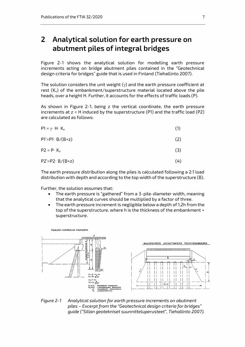
Figure 2-1 shows the analytical solution for modelling earth pressure
increments acting on bridge abutment piles contained in the “Geotechnical
design criteria for bridges” guide that is used in Finland (Tiehallinto 2007).
The solution considers the unit weight () and the earth pressure coefficient at
rest (Ko) of the embankment/superstructure material located above the pile
heads, over a height H. Further, it accounts for the effects of traffic loads (P).
As shown in Figure 2-1, being z the vertical coordinate, the earth pressure
increments at z = H induced by the superstructure (P1) and the traffic load (P2)
are calculated as follows:
P1 = ∙ H∙ Ko (1)
P1’=P1∙ B/(B+z) (2)
P2 = P∙ Ko (3)
P2’=P2∙ B/(B+z) (4)
The earth pressure distribution along the piles is calculated following a 2:1 load
distribution with depth and according to the top width of the superstructure (B).
Further, the solution assumes that:
The earth pressure is “gathered” from a 3-pile-diameter width, meaning
that the analytical curves should be multiplied by a factor of three.
The earth pressure increment is negligible below a depth of 1,2h from the
top of the superstructure, where h is the thickness of the embankment +
superstructure.
Figure 2-1 Analytical solution for earth pressure increments on abutment
piles – Excerpt from the “Geotechnical design criteria for bridges”
guide (“Sillan geotekniset suunnitteluperusteet”, Tiehallinto 2007).
Publications of the FTIA 32/2020 8
3 Definition of problem framework
3.1 Geometries
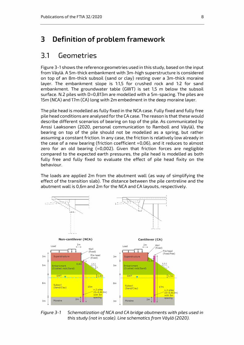
Figure 3-1 shows the reference geometries used in this study, based on the input
from Väylä. A 5m-thick embankment with 3m-high superstructure is considered
on top of an 8m-thick subsoil (sand or clay) resting over a 3m-thick moraine
layer. The embankment slope is 1:1,5 for crushed rock and 1:2 for sand
embankment. The groundwater table (GWT) is set 1,5 m below the subsoil
surface. N.2 piles with D=0,813m are modelled with a 5m-spacing. The piles are
15m (NCA) and 17m (CA) long with 2m embedment in the deep moraine layer.
The pile head is modelled as fully fixed in the NCA case. Fully fixed and fully free
pile head conditions are analysed for the CA case. The reason is that these would
describe different scenarios of bearing on top of the pile. As communicated by
Anssi Laaksonen (2020, personal communication to Ramboll and Väylä), the
bearing on top of the pile should not be modelled as a spring, but rather
assuming a constant friction. In any case, the friction is relatively low already in
the case of a new bearing (friction coefficient ≈0,06), and it reduces to almost
zero for an old bearing (≈0,002). Given that friction forces are negligible
compared to the expected earth pressures, the pile head is modelled as both
fully free and fully fixed to evaluate the effect of pile head fixity on the
behaviour.
The loads are applied 2m from the abutment wall (as way of simplifying the
effect of the transition slab). The distance between the pile centreline and the
abutment wall is 0,6m and 2m for the NCA and CA layouts, respectively.
Figure 3-1 Schematization of NCA and CA bridge abutments with piles used in
this study (not in scale). Line schematics from Väylä (2020).
Publications of the FTIA 32/2020 9
3.2 Loads
The loads considered in this study are:
Traffic loads: 9 kPa distributed, 9+31 (3x5m) kPa - NCCI 7 (FTA guidelines
13/2007)
Train LM-71 max load: 52 (3x6,4m) kPa + 27 kPa (3m width); 52 (3x6,4m) load
on bogies – repeated at 6,1m distance (RATO 3, FTA guidelines 13/2018)
3.3 Calculation matrix
The calculation matrix presented in Table 3-1 summarizes all the different
calculations that are carried out. A progressive number and an ID are assigned
to each calculation, according to the following nomenclature:
Bridge type - Embankment material - Subsoil & Pile-head fixity - Load type
Legend:
Bridge type: CA for cantilever; NCA for non-cantilever
Embankment material: 01 for crushed rock with 1:1,5 slope; 02 for sand with 1:2
slope
Subsoil: S for sand; C for clay
Pile-head fixity: 1 for fully fixed; 2 for fully-free
Load type: T for traffic load (9 + 31 kPa); R1 for distributed 52 kPa+27 kPa LM-71
load; R2 for 52 kPa LM-71 load on bogies
For instance, a cantilever bridge with a crushed rock embankment, clay subsoil,
free pile head and traffic load reads as CA-01-C2-T; whereas a non-cantilever
bridge with a sand embankment, sand subsoil, fixed pile head and distributed
LM-71 load reads as NCA-02-S1-R1.

Publications of the FTIA 32/2020 10
Table 3-1 Calculation matrix.
Bridge type Embankment Subsoil Pile-head fixity Load ID N. Legend
9+31 kPa CA-01-S1-T 1 Crushed rock 01 1:1,5 slope
LM-71 v1 CA-01-S1-R1 2 Sand 02 1:2 slope
LM-71 v2 CA-01-S1-R2 3
Sand S
9+31 kPa CA-01-S2-T 4 Clay C
LM-71 v1 CA-01-S2-R1 5
LM-71 v2 CA-01-S2-R2 6 Fixed 1
Free 2
9+31 kPa CA-01-C1-T 7
LM-71 v1 CA-01-C1-R1 8 Traffic T
LM-71 v2 CA-01-C1-R2 9 Railway R
9+31 kPa CA-01-C2-T 10 Distributed 1
LM-71 v1 CA-01-C2-R1 11 Bogies 2
LM-71 v2 CA-01-C2-R2 12
9+31 kPa CA-02-S1-T 13
LM-71 v1 CA-02-S1-R1 14
LM-71 v2 CA-02-S1-R2 15
9+31 kPa CA-02-S2-T 16
LM-71 v1 CA-02-S2-R1 17
LM-71 v2 CA-02-S2-R2 18
9+31 kPa CA-02-C1-T 19
LM-71 v1 CA-02-C1-R1 20
LM-71 v2 CA-02-C1-R2 21
9+31 kPa CA-02-C2-T 22
LM-71 v1 CA-02-C2-R1 23
LM-71 v2 CA-02-C2-R2 24
9+31 kPa NCA-01-S1-T 25
LM-71 v1 NCA-01-S1-R1 26
LM-71 v2 NCA-01-S1-R2 27
9+31 kPa NCA-01-C1-T 28
LM-71 v1 NCA-01-C1-R1 29
LM-71 v2 NCA-01-C1-R2 30
9+31 kPa NCA-02-S1-T 31
LM-71 v1 NCA-02-S1-R1 32
LM-71 v2 NCA-02-S1-R2 33
9+31 kPa NCA-02-C1-T 34
LM-71 v1 NCA-02-C1-R1 35
LM-71 v2 NCA-02-C1-R1 36
Cantilever
Non-
Cantilever
Free
Fixed
Crushed
rock
Sand
Crushed
rock
Sand
Free
Fixed
Free
Fixed
Free
Fixed
Sand
Clay Fixed
Fixed
Fixed
Fixed
Sand
Clay
Sand
Clay
Sand
Clay
Publications of the FTIA 32/2020 11
4 Finite element model
4.1 Geometry and mesh
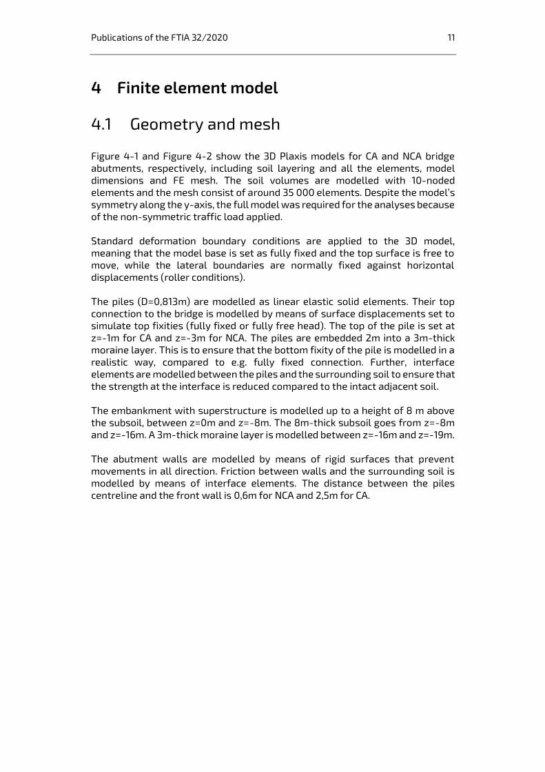
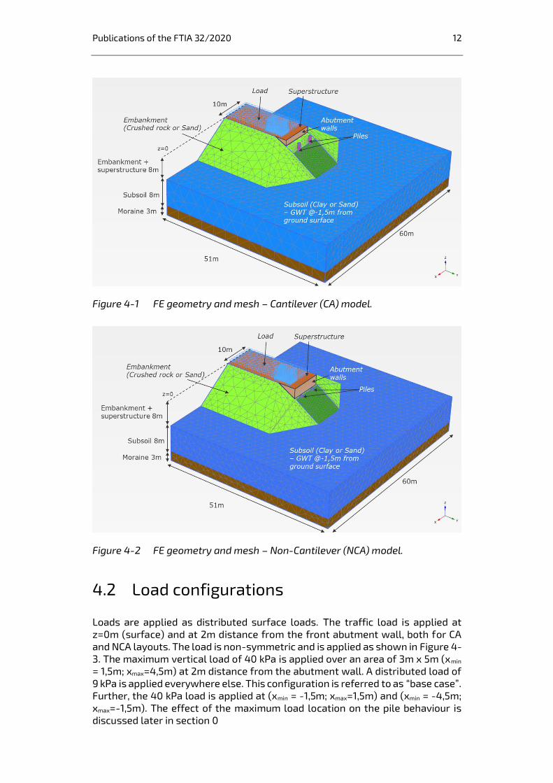
Figure 4-1 and Figure 4-2 show the 3D Plaxis models for CA and NCA bridge
abutments, respectively, including soil layering and all the elements, model
dimensions and FE mesh. The soil volumes are modelled with 10-noded
elements and the mesh consist of around 35 000 elements. Despite the model’s
symmetry along the y-axis, the full model was required for the analyses because
of the non-symmetric traffic load applied.
Standard deformation boundary conditions are applied to the 3D model,
meaning that the model base is set as fully fixed and the top surface is free to
move, while the lateral boundaries are normally fixed against horizontal
displacements (roller conditions).
The piles (D=0,813m) are modelled as linear elastic solid elements. Their top
connection to the bridge is modelled by means of surface displacements set to
simulate top fixities (fully fixed or fully free head). The top of the pile is set at
z=-1m for CA and z=-3m for NCA. The piles are embedded 2m into a 3m-thick
moraine layer. This is to ensure that the bottom fixity of the pile is modelled in a
realistic way, compared to e.g. fully fixed connection. Further, interface
elements are modelled between the piles and the surrounding soil to ensure that
the strength at the interface is reduced compared to the intact adjacent soil.
The embankment with superstructure is modelled up to a height of 8 m above
the subsoil, between z=0m and z=-8m. The 8m-thick subsoil goes from z=-8m
and z=-16m. A 3m-thick moraine layer is modelled between z=-16m and z=-19m.
The abutment walls are modelled by means of rigid surfaces that prevent
movements in all direction. Friction between walls and the surrounding soil is
modelled by means of interface elements. The distance between the piles
centreline and the front wall is 0,6m for NCA and 2,5m for CA.
Publications of the FTIA 32/2020 12
Figure 4-1 FE geometry and mesh – Cantilever (CA) model.
Figure 4-2 FE geometry and mesh – Non-Cantilever (NCA) model.
4.2 Load configurations
Loads are applied as distributed surface loads. The traffic load is applied at
z=0m (surface) and at 2m distance from the front abutment wall, both for CA
and NCA layouts. The load is non-symmetric and is applied as shown in Figure 4-
3. The maximum vertical load of 40 kPa is applied over an area of 3m x 5m (xmin
= 1,5m; xmax=4,5m) at 2m distance from the abutment wall. A distributed load of
9 kPa is applied everywhere else. This configuration is referred to as “base case”.
Further, the 40 kPa load is applied at (xmin = -1,5m; xmax=1,5m) and (xmin = -4,5m;
xmax=-1,5m). The effect of the maximum load location on the pile behaviour is
discussed later in section 0
Publications of the FTIA 32/2020 13
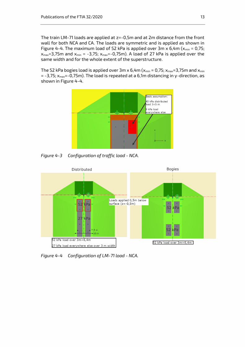
The train LM-71 loads are applied at z=-0,5m and at 2m distance from the front
wall for both NCA and CA. The loads are symmetric and is applied as shown in
Figure 4-4. The maximum load of 52 kPa is applied over 3m x 6,4m (xmin = 0,75;
xmax=3,75m and xmin = -3,75; xmax=-0,75m). A load of 27 kPa is applied over the
same width and for the whole extent of the superstructure.
The 52 kPa bogies load is applied over 3m x 6,4m (xmin = 0,75; xmax=3,75m and xmin
= -3,75; xmax=-0,75m). The load is repeated at a 6,1m distancing in y-direction, as
shown in Figure 4-4.
Figure 4-3 Configuration of traffic load - NCA.
Figure 4-4 Configuration of LM-71 load - NCA.

Publications of the FTIA 32/2020 14
4.3 Construction phases and calculation steps
Figure 4-5 shows the construction phases of the embankment, piles and
superstructure and the calculation steps to model earth pressure on piles under
the different loads for the situation where the subsoil is sand. The initial stresses
in the subsoil are generated through a “Ko phase”, where the soil weight is
applied, and stresses are defined according to Ko.
The 5m embankment is modelled as a drained material and applied by gravity in
a plastic calculation phase (1a). This will result in mobilized shear stress in the
embankment and stress change in the drained subsoil. The mobilized shear in
the embankment is affected by the deformations in the subsoil. In a subsequent
phase (1b), piles are activated. This represents a phase where no mobilization of
earth pressure is generated along the piles, since those are activated (in reality,
installed) only after the embankment construction.
In phase 2, the 3m superstructure and loads are applied. Firstly, the 3m
superstructure, modelled as drained, is applied and the earth pressure mobilized
(2a). Secondly, additional earth pressure mobilization occurs under the applied
load (2b).
Figure 4-6 shows the construction phases of the embankment, piles and super-
structure and the calculation steps to model earth pressure on piles under the
different loads for the situation where the subsoil is clay. The initial stresses in
the subsoil are generated through a “Ko phase”, where the soil weight is applied,
and stresses are defined according to KONC and a POP. The clay is modelled as
Drained.
The 5m embankment is modelled as a drained material and applied by gravity in
a plastic calculation phase (1a). This will result in mobilized shear stress in the
embankment and stress change in the drained subsoil. The mobilized shear in
the embankment is affected by the deformations in the subsoil. Compared to the
sand case, the embankment deformations are anticipated to be significantly
larger (≈2 orders or magnitude). In a subsequent phase (1b), piles are activated.
This represents a phase where no mobilization of earth pressure is generated
along the piles, since those are activated (in reality, installed) only after the
embankment construction.
In phase 2, the clay behaviour is switched to undrained and 3m superstructure
and loads are applied. Firstly, the 3m superstructure, modelled as drained, is
applied and the earth pressure mobilized both from the embankment and the
undrained clay (2a). Secondly, additional earth pressure mobilization occurs
under the applied load (2b).

Publications of the FTIA 32/2020 15
Figure 4-5 Calculation steps – Sand subsoil (not in scale).
Figure 4-6 Calculation steps – Clay subsoil (not in scale).
4.4 Earth pressure modelling
The earth pressure along the piles is modelled as the average stress acting on a
surface right behind the pile. The surface width is taken equal to the pile
diameter D = 0,813 m. The reference surface is normal to the maximum
displacement direction, which is inclined by an angle from the x-direction. The
concept is illustrated in Figure 4-7:
Publications of the FTIA 32/2020 16
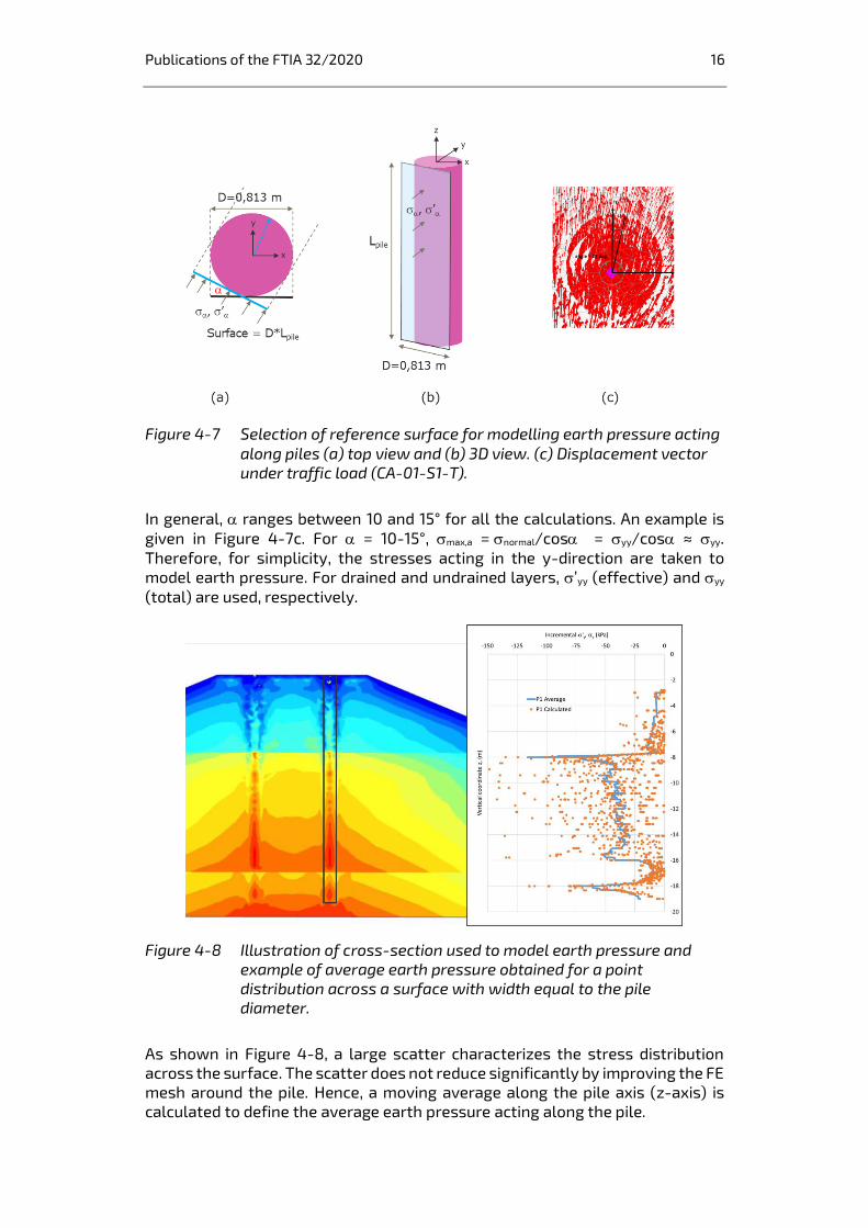
Figure 4-7 Selection of reference surface for modelling earth pressure acting
along piles (a) top view and (b) 3D view. (c) Displacement vector
under traffic load (CA-01-S1-T).
In general, ranges between 10 and 15° for all the calculations. An example is
given in Figure 4-7c. For = 10-15°, max,a =normal/cos = yy/cos ≈ yy.
Therefore, for simplicity, the stresses acting in the y-direction are taken to
model earth pressure. For drained and undrained layers, ’yy (effective) and yy
(total) are used, respectively.
Figure 4-8 Illustration of cross-section used to model earth pressure and
example of average earth pressure obtained for a point
distribution across a surface with width equal to the pile
diameter.
As shown in Figure 4-8, a large scatter characterizes the stress distribution
across the surface. The scatter does not reduce significantly by improving the FE
mesh around the pile. Hence, a moving average along the pile axis (z-axis) is
calculated to define the average earth pressure acting along the pile.
Publications of the FTIA 32/2020 17
5 Material models and parameters
Coarse materials that are expected to exhibit drained behaviour are modelled by
the Hardening Soil model. These include the embankment, superstructure, sand
subsoil and moraine. The Hardening Soil model is further used to simulate the
long-term drained behaviour of the clay subsoil beneath the 5m embankment,
prior to construction of the superstructure and application of the loads. The
undrained behaviour of the clay subsoil is otherwise modelled by the Mohr-
Coulomb model where the stiffness is selected so that it corresponds to fairy
small strain levels. Piles are modelled as linear elastic volume elements. The
following sections describe the basics of the material models used and the
selection of model parameters.
Input parameters to the FE analyses are selected based on inputs from the
Client, available literature and Ramboll’s experience. The proposed parameters
are anticipated to represent best estimate properties.
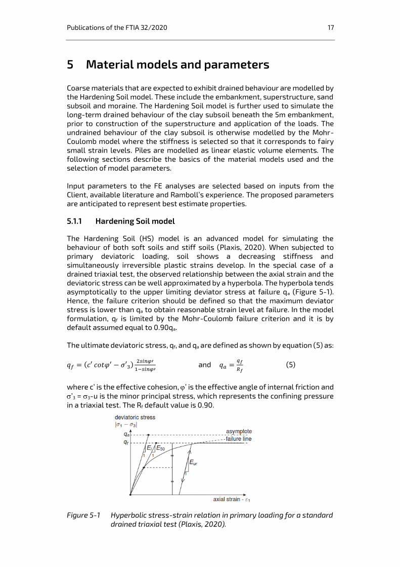
5.1.1 Hardening Soil model
The Hardening Soil (HS) model is an advanced model for simulating the
behaviour of both soft soils and stiff soils (Plaxis, 2020). When subjected to
primary deviatoric loading, soil shows a decreasing stiffness and
simultaneously irreversible plastic strains develop. In the special case of a
drained triaxial test, the observed relationship between the axial strain and the
deviatoric stress can be well approximated by a hyperbola. The hyperbola tends
asymptotically to the upper limiting deviator stress at failure qa (Figure 5-1).
Hence, the failure criterion should be defined so that the maximum deviator
stress is lower than qa to obtain reasonable strain level at failure. In the model
formulation, qf is limited by the Mohr-Coulomb failure criterion and it is by
default assumed equal to 0.90qa.
The ultimate deviatoric stress, qf, and qa are defined as shown by equation (5) as:
𝑞𝑓 = (𝑐′ 𝑐𝑜𝑡𝜑′ − 𝜎′3)2𝑠𝑖𝑛𝜑′
1−𝑠𝑖𝑛𝜑′ and 𝑞𝑎 =
𝑞𝑓
𝑅𝑓 (5)
where c’ is the effective cohesion, ’ is the effective angle of internal friction and
’3 = 3-u is the minor principal stress, which represents the confining pressure
in a triaxial test. The Rf default value is 0.90.
Figure 5-1 Hyperbolic stress-strain relation in primary loading for a standard
drained triaxial test (Plaxis, 2020).
Publications of the FTIA 32/2020 18
Some basic characteristics of the model are:
Stress dependent stiffness according to a power law
Input parameter m
Plastic straining due to primary deviatoric loading
Input parameter E50ref
Plastic straining due to primary compression
Input parameter Eoedref
Elastic unloading / reloading
Input parameters Eurref, ur
Failure according to the Mohr-Coulomb failure criterion
Parameters c’, ’ and
A basic feature of the HS model is the stress dependency of soil stiffness. For
oedometer conditions of stress and strain, the model implies for example the
relationship:
Eoed = Eoedref (’ / pref)m (6)
where Eoed is the oedometer modulus at a given stress level ’, Eoed is the
oedometer modulus at a reference stress pref (a default pref = 100 kPa is used by
Plaxis), m is the stress exponent defined as 1 – (being the Ohde-Janbu’s stress
exponent). The stiffness in primary drained triaxial loading E50 and the
unloading/reloading stiffness Eur are defined in a similar way as Eoed. More
details can be found in the Plaxis’ user’s manual (Plaxis, 2020).
Typically, m ≈ 0,5 for coarse soils, while m ≈ 0,7 for silty soils. In the special case
of soft soils, it is realistic to use m = 1.
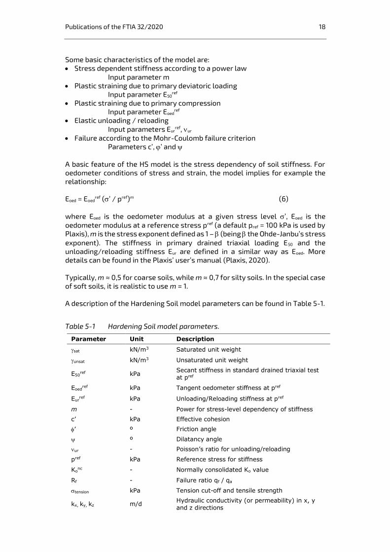
A description of the Hardening Soil model parameters can be found in Table 5-1.
Table 5-1 Hardening Soil model parameters.
Parameter Unit Description
sat kN/m3 Saturated unit weight
unsat kN/m3 Unsaturated unit weight
E50ref kPa
Secant stiffness in standard drained triaxial test at pref
Eoedref kPa Tangent oedometer stiffness at pref
Eurref kPa Unloading/Reloading stiffness at pref
m - Power for stress-level dependency of stiffness
c’ kPa Effective cohesion
’ º Friction angle
º Dilatancy angle
ur - Poisson’s ratio for unloading/reloading
pref kPa Reference stress for stiffness
Konc - Normally consolidated Ko value
Rf - Failure ratio qf / qa
tension kPa Tension cut-off and tensile strength
kx, ky, kz m/d Hydraulic conductivity (or permeability) in x, y and z directions
Publications of the FTIA 32/2020 19
Parameter Unit Description
e0 - Initial void ratio
ck - Change of permeability coefficient
POP kPa Pre-overburden pressure
Rinter - Interface strength reduction coefficient
Generally, the symbol m is used to indicate the Ohde-Jabu’s modulus number;
while in the HS model, m represents the stress-exponent (= 1 – ). To avoid
confusion, the modulus number is hereinafter indicated using the symbol m*,
while m is kept for the stress exponent. Hence, the stress-dependent moduli can
be determined as shown in equations (7), (8) and (9) as:
Eoedref = m*∙ pref (7)
E50ref ≈ Eoed
ref (8)
Eurref = n∙ E50
ref (9)
As described in the PLAXIS’ manual, in many practical cases it is appropriate to
set Eurref equal to 3E50
ref; this is the default setting used in PLAXIS. Further, it is
generally assumed that E50ref ≈ Eoed
ref. However, the ratio between moduli should
be defined based on laboratory test results, whenever possible. For the
superstructure, Eurref = 2E50
ref is assumed. For clay, Eurref > 10E50
ref.
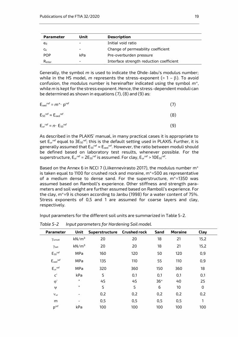
Based on the Annex 6 in NCCI 7 (Liikennevirasto 2017), the modulus number m*
is taken equal to 1100 for crushed rock and moraine, m*=500 as representative
of a medium dense to dense sand. For the superstructure, m*=1350 was
assumed based on Ramboll’s experience. Other stiffness and strength para-
meters and soil weight are further assumed based on Ramboll’s experience. For
the clay, m*=9 is chosen according to Janbu (1998) for a water content of 75%.
Stress exponents of 0,5 and 1 are assumed for coarse layers and clay,
respectively.
Input parameters for the different soil units are summarized in Table 5-2.
Table 5-2 Input parameters for Hardening Soil model.
Parameter Unit Superstructure Crushed rock Sand Moraine Clay
unsat kN/m³ 20 20 18 21 15,2
sat kN/m³ 20 20 18 21 15,2
E50ref MPa 160 120 50 120 0,9
Eoedref MPa 135 110 55 110 0,9
Eurref MPa 320 360 150 360 18
c' kPa 5 0,1 0,1 0,1 0,1
' ° 45 45 36* 40 25
° 5 5 6 10 0
ur - 0,2 0,2 0,2 0,2 0,2
m - 0,5 0,5 0,5 0,5 1
pref kPa 100 100 100 100 100

Publications of the FTIA 32/2020 20
Parameter Unit Superstructure Crushed rock Sand Moraine Clay
K0nc - 0,29 0,33 0,41 0,36 0,58
Rf - 0,9 0,9 0,9 0,9 0,9
e - 0,5 0,5 0,5 0,5 2
POP kPa 0 0 0 0 20
Rinter - 0,5 0,5 0,5 0,5 0,7
Drainage type - Drained Drained Drained Drained Drained
*Input from the Client
5.1.2 Mohr-Coulomb model
The Mohr-Coulomb (MC) model is an elastoplastic model for simulating both
drained and undrained soil behaviour. The model assumes a constant stiffness
and a linear-stress-strain behaviour before reaching the failure state. In this
way, the stiffness is independent of both stress level and shear mobilization. The
MC model is used to model the undrained response of the clay subsoil. As
suggested by the Client, the 8m-thick clay unit is characterized by a constant
undrained shear strength su = 40 kPa. The soil stiffness is then selected
according to literature as a function of su and assuming a plasticity index (PI) of
30%.
According to Termaat et al. (1985), the shear modulus at 50% of the shear
strength (G50) can be defined as:
G50/su = 5000/PI(%) = 5000/30 ≈ 167 (10)
Further, a common formula to estimate the undrained elastic modulus Eu is:
Eu/su = 15000/PI(%) = 15000/30 = 500 (11)
Equations (10) and (11) give G = 6680 kPa and Eu = 20 000 kPa. The elasticity
theory suggests that for Eu = 20 000 kPa and =0,495 (undrained), G = 6689 kPa.
This is in line with equation (10).
Table 5-3 summarizes the input parameters for the Mohr-Coulomb model.
Table 5-3 Input parameters for Mohr-Coulomb model.
Parameter unsat sat su G/su Eu/su G Eu Rinter Drainage
type
Unit kN/m³ kN/m³ kPa - - MPa MPa - - -
Clay 15,2 15,2 40* 167 500 6,7 20 0,495 0,7 Undrained
(C) *Input from the Client
5.1.3 Linear Elastic parameters for piles
The piles are modelled as circular linear elastic volume elements with an elastic
modulus E = 42 GPa, Poisson’s ratio = 0,3, unit weight = 28 kN/m3 and
diameter D = 0,813 m.
The input parameters are calculated for composite reinforced concrete
RR800/12.5 piles with steel grade S440J2H. The pile is characterized by a steel
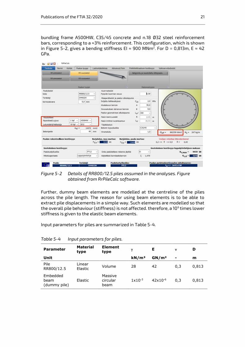
Publications of the FTIA 32/2020 21
bundling frame A500HW, C35/45 concrete and n.18 Ø32 steel reinforcement
bars, corresponding to a ≈3% reinforcement. This configuration, which is shown
in Figure 5-2, gives a bending stiffness EI ≈ 900 MNm2. For D = 0,813m, E ≈ 42
GPa.
Figure 5-2 Details of RR800/12.5 piles assumed in the analyses. Figure
obtained from RrPileCalc software.
Further, dummy beam elements are modelled at the centreline of the piles
across the pile length. The reason for using beam elements is to be able to
extract pile displacements in a simple way. Such elements are modelled so that
the overall pile behaviour (stiffness) is not affected. therefore, a 106 times lower
stiffness is given to the elastic beam elements.
Input parameters for piles are summarized in Table 5-4.
Table 5-4 Input parameters for piles.
Parameter Material type
Element type
E D
Unit kN/m³ GN/m² - m
Pile RR800/12.5
Linear Elastic
Volume 28 42 0,3 0,813
Embedded beam (dummy pile)
Elastic Massive circular beam
1x10⁻³ 42x10-6 0,3 0,813
Publications of the FTIA 32/2020 22
6 Results
6.1 Model performance and behaviour
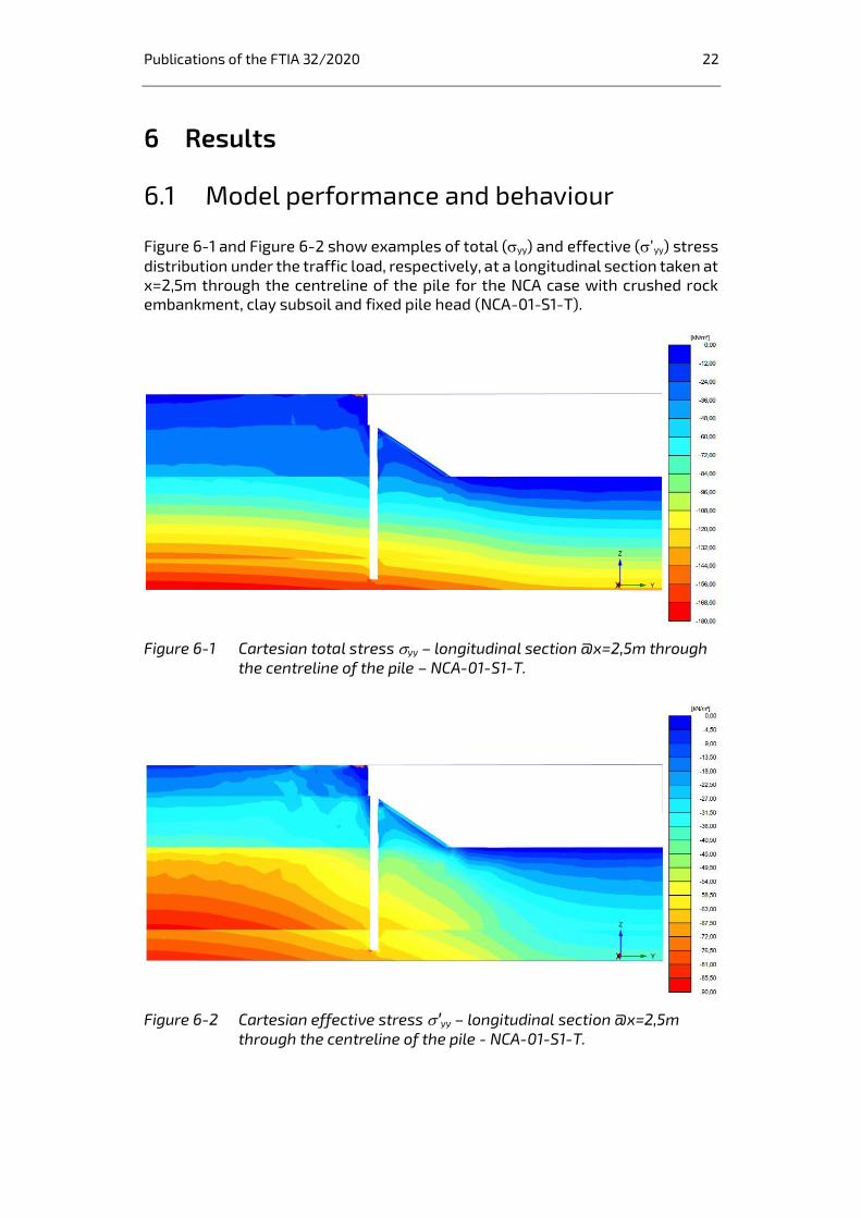
Figure 6-1 and Figure 6-2 show examples of total (yy) and effective (’yy) stress
distribution under the traffic load, respectively, at a longitudinal section taken at
x=2,5m through the centreline of the pile for the NCA case with crushed rock
embankment, clay subsoil and fixed pile head (NCA-01-S1-T).
Figure 6-1 Cartesian total stress yy – longitudinal section @x=2,5m through
the centreline of the pile – NCA-01-S1-T.
Figure 6-2 Cartesian effective stress 'yy – longitudinal section @x=2,5m
through the centreline of the pile - NCA-01-S1-T.

Publications of the FTIA 32/2020 23
Figure 6-3 and Figure 6-4 show examples of total displacements for NCA-01-S1-
T (sand subsoil) and NCA-01-C1-T, respectively, under the traffic load at the
same longitudinal section. It can be noted that the traffic load produces a
maximum displacement at surface (settlement) of ≈3-4mm. According to
Väylävirasto, this is in line with what is typically observed and somewhat
validates the stiffness of the FE model. Further, displacements under the LM-71
loads are ≈4mm for the case with sand subsoil and ≈6,5mm for the case with
clay subsoil. Similar values were found in all the other NCA and CA cases
analysed. The computed displacements were found to be substantially
independent of the FE mesh used.
Figure 6-3 Phase displacement - Load application (Phase 2b) – longitudinal
section @x=2,5m through the centreline of the pile – NCA-01-S1-T.
Figure 6-4 Phase displacement - Load application (Phase 2b) – longitudinal
section @x=2,5m through the centreline of the pile – NCA-01-C1-T.

Publications of the FTIA 32/2020 24
6.2 Mesh sensitivity check
The sensitivity of FE results to the element discretization is checked for the pile
horizontal displacement under the traffic load. As shown in Figure 6-5, the use
of a Very Fine mesh, consisting of approximately 130 000 elements, does not
show a significant increase of displacements (less than 1%) compared to the
Very Coarse (≈ 19 000 elements) and Medium (≈ 35 000 elements) mesh types.
This is true for both CA and NCA configurations and for both clay and sand
subsoil. Further, the use of a Very fine mesh increases significantly the
computation time. Therefore, the Medium mesh is used in subsequent analyses.
Figure 6-5 Sensitivity of pile displacements to the FE mesh.
6.3 Effect of traffic load configuration
The impact of load traffic asymmetry is checked in Figure 6-6 by comparing pile
displacement of the reference pile for different load configurations, i.e. by
changing the location of the maximum load (40 kPa over 3m x 5m). The
differences in terms of displacements of the reference pile are less than 1%. As
expected, the pile displacement increases more significantly when a load of
40 kPa is applied to the whole loading area.
As shown in Figure 6-6, the location of the maximum load does not have any
notable effect on pile behaviour. Such a conclusion is anticipated to be valid for
all NCA and CA cases and regardless of the subsoil and/or embankment material.
Therefore, the “load on right” configuration is taken as the base case
configuration to model earth pressure under traffic load.

Publications of the FTIA 32/2020 25
Figure 6-6 Effect of traffic load configuration on pile displacements (NCA-01-
S1-T).
6.4 Earth pressure: FEM vs analytical solution
Figure 6-7 to Figure 6-19 show a comparison between the computed earth
pressure under traffic and LM-71 loads and the analytical solutions for P1 and
P2. The analytical curves do not include the assumed multiplying factor of 3
that accounts for gathering of earth pressure from an area equal to 3 times
the pile diameter (see section 0). The two analysed LM-71 load configurations
(distributed and bogies) give substantially similar results, as shown in Figure 6-
7 and Figure 6-8. Therefore, only the “52 kPa + 27 kPa” LM-71 load results are
presented in Figure 6-9 to Figure 6-19 together with the “9 kPa + 31 kPa” traffic
load.
In the analytical solution for P2, average traffic/train loads are selected to model
P and P2 in equations (3) and (4). In detail, P = 10 kPa with B = 10 m and P = 32 kPa
with B = 7,5 m are selected for traffic load and LM-71 load, respectively.
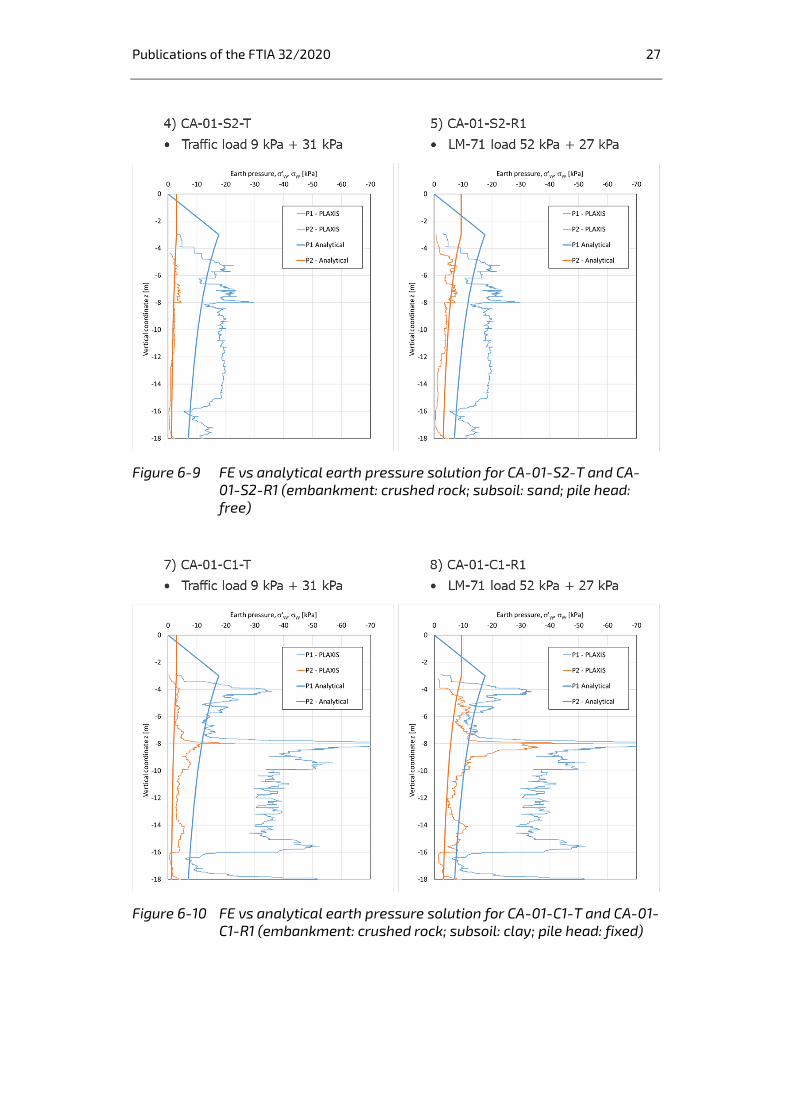
In most cases, the analytical solution appears to deviate from the FE results. In
particular, it severely underestimates the earth pressure in undrained
conditions. The analytical solution seems to be more in line with the earth
pressure in the coarse layers when the model is governed by drained conditions
(i.e. sand subsoil). Nevertheless, the solution is based on Ko conditions and it only
accounts for the Ko of the superstructure. On the other hand, the mobilized earth
pressure may deviate from Ko conditions according to the degree of mobilization.
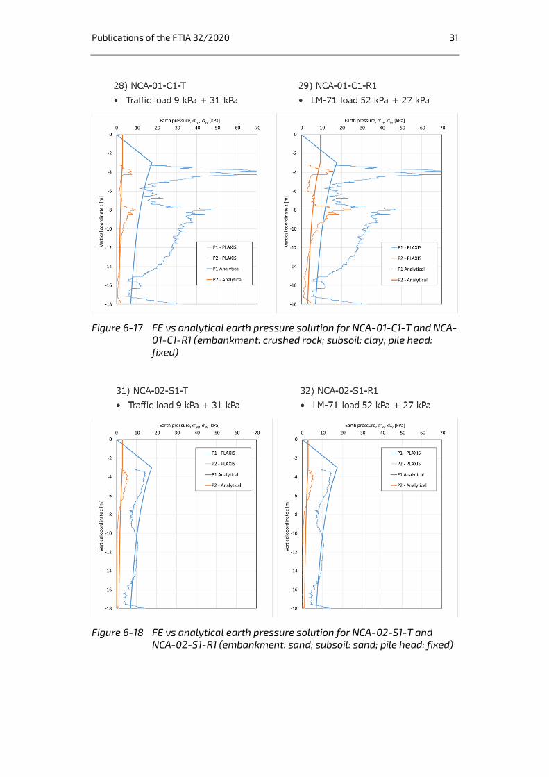
In undrained conditions, the two solutions show a discrepancy even in the coarse
layers, especially for the NCA cases with clay subsoil (see Figure 6-17 and Figure
6-19). One possible reason may be the high shear mobilization in the
embankment that results from the simulation of long-term conditions (large
settlement after construction). In this way, the embankment and superstructure
will show a softer behaviour compared to the case with sand subsoil, with
consequent stress concentration and earth pressure increase behind the fixed

Publications of the FTIA 32/2020 26
piles. This behaviour seems to be less pronounced in the CA model with fixed pile
head (Figure 6-10 and Figure 6-14), while it tends to disappear when the pile
head is free to move (Figure 6-11 and Figure 6-15). It must be noted that the
distance between the centre of the pile and the abutment wall is larger in the CA
model (2,5m) compared to the NCA model (0,6m).
Figure 6-7 FE vs analytical earth pressure solution for CA-01-S1-T and CA-01-
S1-R1 (embankment: crushed rock; subsoil: sand; pile head: fixed)
Figure 6-8 FE vs analytical earth pressure solution for CA-01-S1-R2
(embankment: crushed rock; subsoil: sand; pile head: fixed)
Publications of the FTIA 32/2020 27
Figure 6-9 FE vs analytical earth pressure solution for CA-01-S2-T and CA-
01-S2-R1 (embankment: crushed rock; subsoil: sand; pile head:
free)
Figure 6-10 FE vs analytical earth pressure solution for CA-01-C1-T and CA-01-
C1-R1 (embankment: crushed rock; subsoil: clay; pile head: fixed)

Publications of the FTIA 32/2020 28
Figure 6-11 FE vs analytical earth pressure solution for CA-01-C2-T and CA-
01-C2-R1 (embankment: crushed rock; subsoil: clay; pile head:
free)
Figure 6-12 FE vs analytical earth pressure solution for CA-02-S1-T and CA-
02-S1-R1 (embankment: sand; subsoil: sand; pile head: fixed)

Publications of the FTIA 32/2020 29
Figure 6-13 FE vs analytical earth pressure solution for CA-02-S2-T and CA-
02-S2-R1 (embankment: sand; subsoil: sand; pile head: free)
Figure 6-14 FE vs analytical earth pressure solution for CA-02-C1-T and CA-
02-C1-R1 (embankment: sand; subsoil: clay; pile head: fixed)

Publications of the FTIA 32/2020 30
Figure 6-15 FE vs analytical earth pressure solution for CA-02-C2-T and CA-
02-C2-R1 (embankment: sand; subsoil: clay; pile head: free)
Figure 6-16 FE vs analytical earth pressure solution for NCA-01-S1-T and NCA-
01-S1-R1 (embankment: crushed rock; subsoil: sand; pile head:
fixed)
Publications of the FTIA 32/2020 31
Figure 6-17 FE vs analytical earth pressure solution for NCA-01-C1-T and NCA-
01-C1-R1 (embankment: crushed rock; subsoil: clay; pile head:
fixed)
Figure 6-18 FE vs analytical earth pressure solution for NCA-02-S1-T and
NCA-02-S1-R1 (embankment: sand; subsoil: sand; pile head: fixed)
Publications of the FTIA 32/2020 32
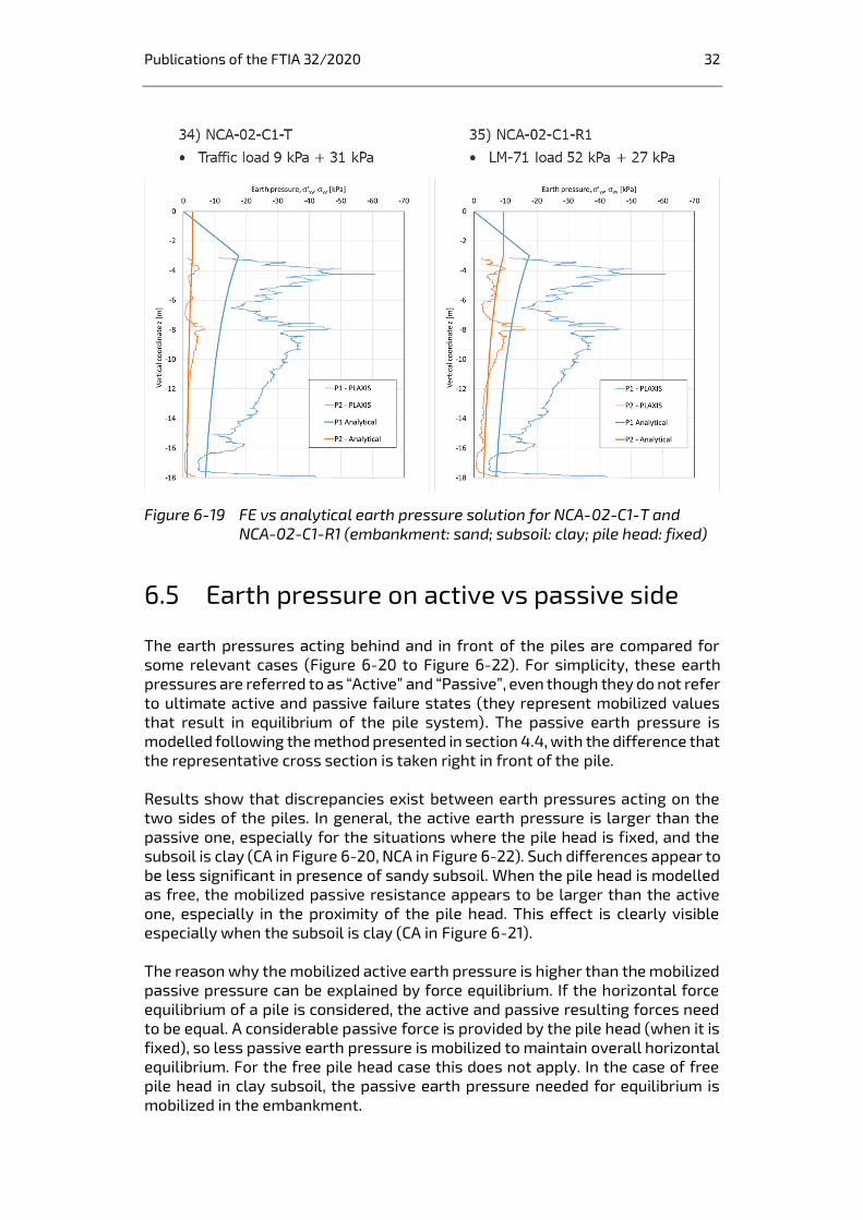
Figure 6-19 FE vs analytical earth pressure solution for NCA-02-C1-T and
NCA-02-C1-R1 (embankment: sand; subsoil: clay; pile head: fixed)
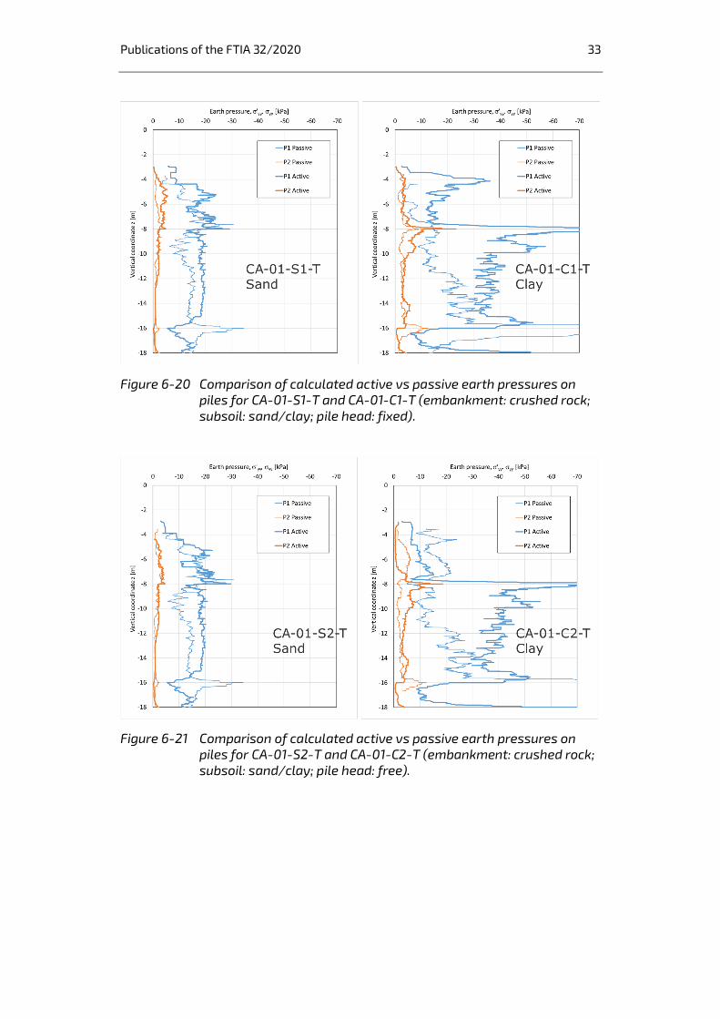
6.5 Earth pressure on active vs passive side
The earth pressures acting behind and in front of the piles are compared for
some relevant cases (Figure 6-20 to Figure 6-22). For simplicity, these earth
pressures are referred to as “Active” and “Passive”, even though they do not refer
to ultimate active and passive failure states (they represent mobilized values
that result in equilibrium of the pile system). The passive earth pressure is
modelled following the method presented in section 4.4, with the difference that
the representative cross section is taken right in front of the pile.
Results show that discrepancies exist between earth pressures acting on the
two sides of the piles. In general, the active earth pressure is larger than the
passive one, especially for the situations where the pile head is fixed, and the
subsoil is clay (CA in Figure 6-20, NCA in Figure 6-22). Such differences appear to
be less significant in presence of sandy subsoil. When the pile head is modelled
as free, the mobilized passive resistance appears to be larger than the active
one, especially in the proximity of the pile head. This effect is clearly visible
especially when the subsoil is clay (CA in Figure 6-21).
The reason why the mobilized active earth pressure is higher than the mobilized
passive pressure can be explained by force equilibrium. If the horizontal force
equilibrium of a pile is considered, the active and passive resulting forces need
to be equal. A considerable passive force is provided by the pile head (when it is
fixed), so less passive earth pressure is mobilized to maintain overall horizontal
equilibrium. For the free pile head case this does not apply. In the case of free
pile head in clay subsoil, the passive earth pressure needed for equilibrium is
mobilized in the embankment.
Publications of the FTIA 32/2020 33
Figure 6-20 Comparison of calculated active vs passive earth pressures on
piles for CA-01-S1-T and CA-01-C1-T (embankment: crushed rock;
subsoil: sand/clay; pile head: fixed).
Figure 6-21 Comparison of calculated active vs passive earth pressures on
piles for CA-01-S2-T and CA-01-C2-T (embankment: crushed rock;
subsoil: sand/clay; pile head: free).

Publications of the FTIA 32/2020 34
Figure 6-22 Comparison of calculated active vs passive earth pressures on
piles for NCA-01-S1-T and NCA-01-C1-T (embankment: crushed
rock; subsoil: sand/clay; pile head: fixed).
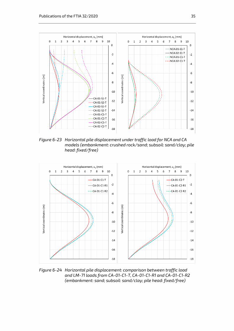
6.6 Pile displacements
Figure 6-23 illustrates the computed horizontal pile displacement (uy) from the
combined superstructure and traffic load for the different NCA and CA models.
For the CA cases with sand subsoil, uy_max ≈ 1,5-2,5 mm; while in presence of clay
subsoil uy_max ≈ 6,5-7,5 mm. For the NCA cases with sand subsoil, uy_max ≈ 1-1,3 mm;
while in presence of clay subsoil uy_max ≈ 5,5-6 mm.
In general, uy in clay is about 5-6 times than uy in sand. The maximum calculated
horizontal pile head displacement is 5,5 mm and is obtained from the CA case
with sand embankment and clay subsoil.
Figure 6-24 compares uy under traffic and LM-71 loads for the CA models with
crushed rock embankments and clay subsoil. The value of uy_max increases by ≈1
mm under the LM-71 load. Similar results are obtained for all the other CA and
NCA models.
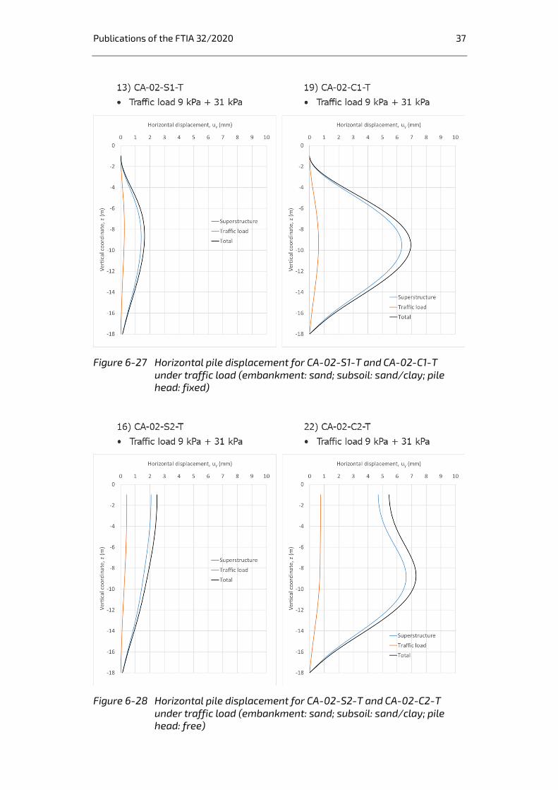
Figure 6-25 to Figure 6-30 show uy from the different calculation phases. The
sole traffic load phase generates a displacement of less than 1 mm. Most of the
deformations and, hence, earth pressure, appear to derive from the super-
structure construction phase.
In conclusion, traffic (road or railway) loading seems to cause approximately
10% of the total pile movement when the pile head is modelled as fixed; while it
causes approximately 15-20% of the total pile movement in the upper part of the
pile with free head.
Publications of the FTIA 32/2020 35
Figure 6-23 Horizontal pile displacement under traffic load for NCA and CA
models (embankment: crushed rock/sand; subsoil: sand/clay; pile
head: fixed/free)
Figure 6-24 Horizontal pile displacement: comparison between traffic load
and LM-71 loads from CA-01-C1-T, CA-01-C1-R1 and CA-01-C1-R2
(embankment: sand; subsoil: sand/clay; pile head: fixed/free)

Publications of the FTIA 32/2020 36
Figure 6-25 Horizontal pile displacement for CA-01-S1-T and CA-01-C1-T under
traffic load (embankment: crushed rock; subsoil: sand/clay; pile
head: fixed)
Figure 6-26 Horizontal pile displacement for CA-01-S2-T and CA-01-C2-T
under traffic load (embankment: crushed rock; subsoil: sand/clay;
pile head: free)
Publications of the FTIA 32/2020 37
Figure 6-27 Horizontal pile displacement for CA-02-S1-T and CA-02-C1-T
under traffic load (embankment: sand; subsoil: sand/clay; pile
head: fixed)
Figure 6-28 Horizontal pile displacement for CA-02-S2-T and CA-02-C2-T
under traffic load (embankment: sand; subsoil: sand/clay; pile
head: free)

Publications of the FTIA 32/2020 38
Figure 6-29 Horizontal pile displacement for NCA-01-S1-T and NCA-01-C1-T
under traffic load (embankment: crushed rock; subsoil: sand/clay;
pile head: fixed)
Figure 6-30 Horizontal pile displacement for NCA-02-S1-T and NCA-02-C1-T
under traffic load (embankment: sand; subsoil: sand/clay; pile
head: fixed)

Publications of the FTIA 32/2020 39
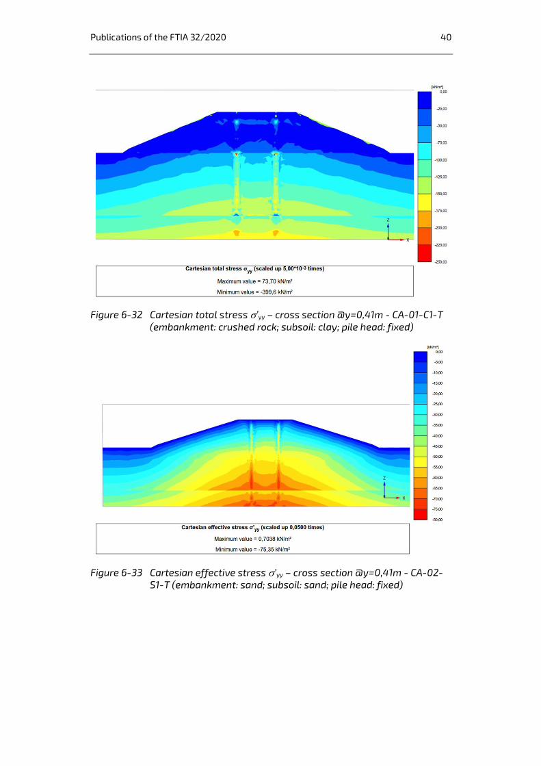
6.7 Earth pressure distribution
Figure 6-31 to Figure 6-38 show the earth pressure distribution under the traffic
load acting on a cross section taken right behind the piles at y=-0,41m. Since the
cross section is normal to the y-axis, the normal stress to the surface
corresponds to ’yy (effective) or yy (total).
Figure 6-31 and Figure 6-33 suggest a 5-10 kPa difference in the sand subsoil
between the earth pressure on the piles and the soil between piles. Such a
difference is ≈25 kPa in both crushed rock and sand embankment. Similar results
are obtained for the free pile-head configurations and for the LM-71 loads.
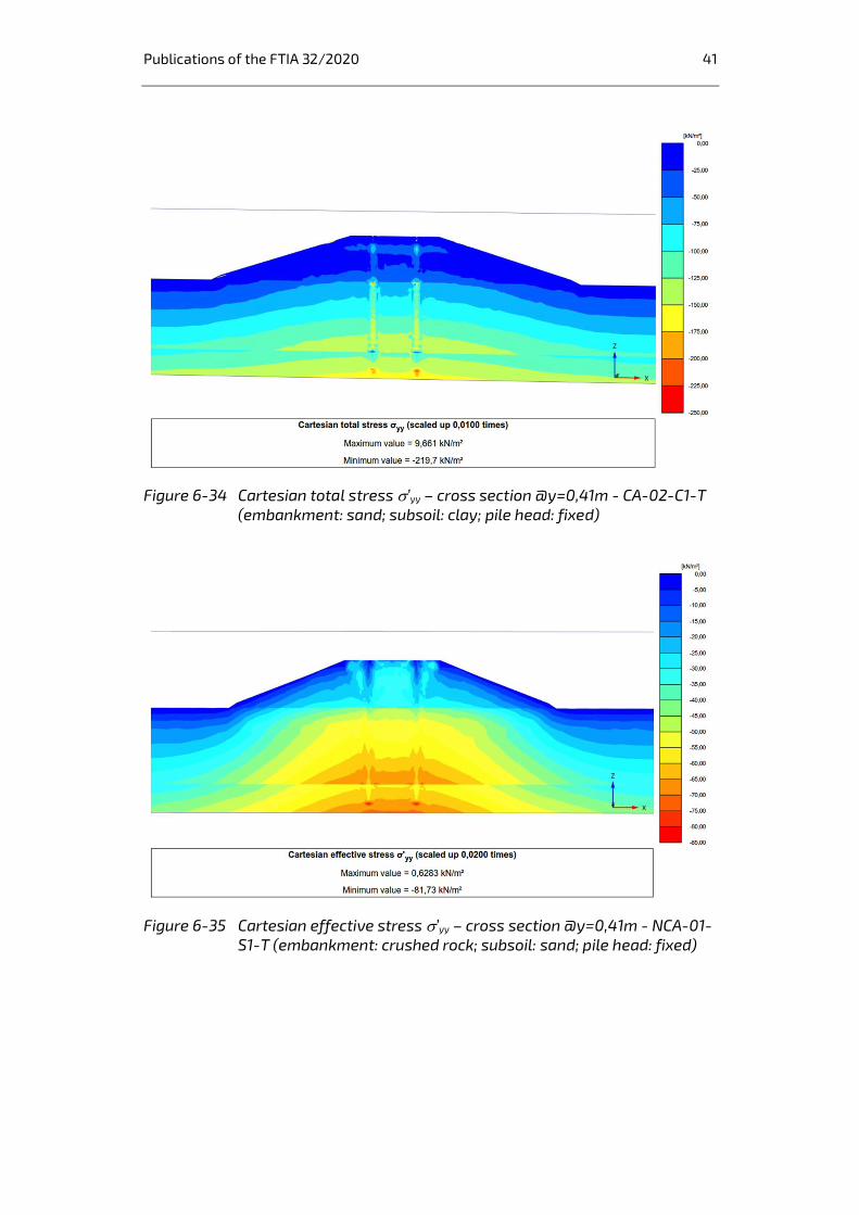
Figure 6-32 and Figure 6-34 suggest a ≈25 kPa difference in the clay subsoil
between the earth pressure on the piles and the soil between piles. Such a
difference is ≈25-50 kPa in the crushed rock and up to ≈25 kPa in the sand
embankment. Similar results are obtained for the free pile-head configurations
and for the LM-71 loads.
Figure 6-35 and Figure 6-37 suggest a ≈5 kPa difference in the sand subsoil
between the earth pressure on the piles and the soil between piles. Such a
difference is ≈10 kPa in the crushed rock and ≈0-5 kPa in the sand embankment.
Similar results are obtained for the LM-71 loads.
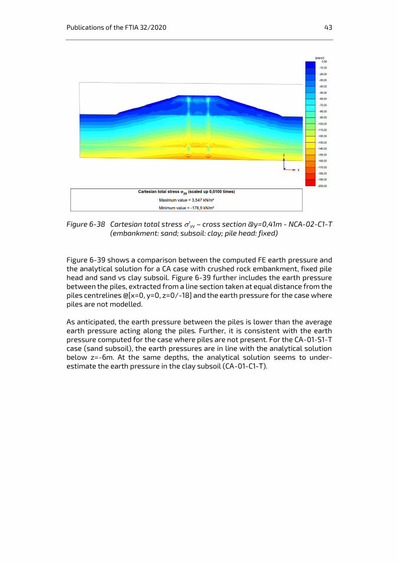
Figure 6-36 and Figure 6-38 suggest a ≈10-30 kPa difference in the clay subsoil
between the earth pressure on the piles and the soil between piles. Such a
difference is ≈10 kPa in the crushed rock and ≈10-25 kPa in the sand
embankment. Similar results are obtained for the LM-71 loads.
Figure 6-31 Cartesian effective stress ’yy – cross section @y=0,41m - CA-01-
S1-T (embankment: crushed rock; subsoil: sand; pile head: fixed)
Publications of the FTIA 32/2020 40
Figure 6-32 Cartesian total stress ’yy – cross section @y=0,41m - CA-01-C1-T
(embankment: crushed rock; subsoil: clay; pile head: fixed)
Figure 6-33 Cartesian effective stress ’yy – cross section @y=0,41m - CA-02-
S1-T (embankment: sand; subsoil: sand; pile head: fixed)
Publications of the FTIA 32/2020 41
Figure 6-34 Cartesian total stress ’yy – cross section @y=0,41m - CA-02-C1-T
(embankment: sand; subsoil: clay; pile head: fixed)
Figure 6-35 Cartesian effective stress ’yy – cross section @y=0,41m - NCA-01-
S1-T (embankment: crushed rock; subsoil: sand; pile head: fixed)

Publications of the FTIA 32/2020 42
Figure 6-36 Cartesian total stress ’yy – cross section @y=0,41m - NCA-01-C1-T
(embankment: crushed rock; subsoil: clay; pile head: fixed)
Figure 6-37 Cartesian effective stress ’yy – cross section @y=0,41m - NCA-02-
S1-T (embankment: sand; subsoil: sand; pile head: fixed)
Publications of the FTIA 32/2020 43
Figure 6-38 Cartesian total stress ’yy – cross section @y=0,41m - NCA-02-C1-T
(embankment: sand; subsoil: clay; pile head: fixed)
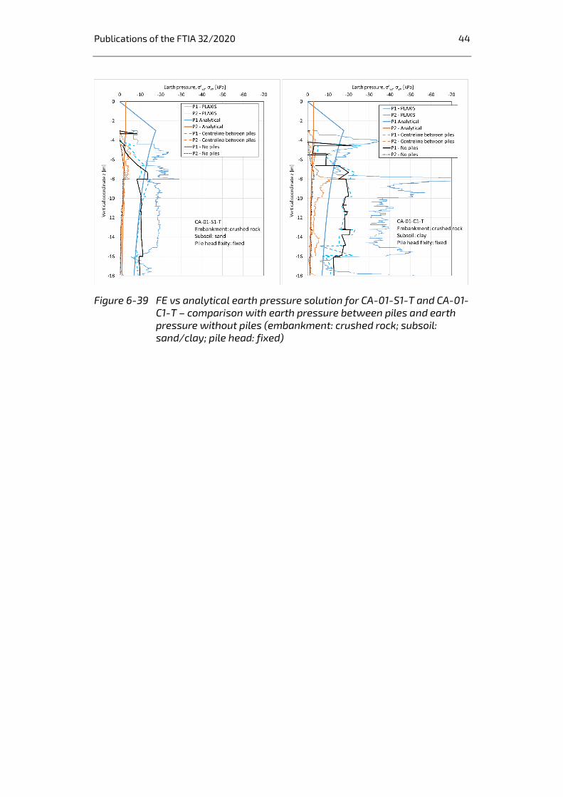
Figure 6-39 shows a comparison between the computed FE earth pressure and
the analytical solution for a CA case with crushed rock embankment, fixed pile
head and sand vs clay subsoil. Figure 6-39 further includes the earth pressure
between the piles, extracted from a line section taken at equal distance from the
piles centrelines @[x=0, y=0, z=0/-18] and the earth pressure for the case where
piles are not modelled.
As anticipated, the earth pressure between the piles is lower than the average
earth pressure acting along the piles. Further, it is consistent with the earth
pressure computed for the case where piles are not present. For the CA-01-S1-T
case (sand subsoil), the earth pressures are in line with the analytical solution
below z=-6m. At the same depths, the analytical solution seems to under-
estimate the earth pressure in the clay subsoil (CA-01-C1-T).
Publications of the FTIA 32/2020 44
Figure 6-39 FE vs analytical earth pressure solution for CA-01-S1-T and CA-01-
C1-T – comparison with earth pressure between piles and earth
pressure without piles (embankment: crushed rock; subsoil:
sand/clay; pile head: fixed)

Publications of the FTIA 32/2020 45
7 Improvement of analytical solutions for
earth pressure
The FE results seems to suggest that the current analytical approach does not
provide with a realistic estimate of earth pressure increments, especially in
undrained conditions. An attempt to improve the current analytical solution is
presented here.
A new set of equations for earth pressure increments P1 and P2 is proposed as
follows (equations (12)-(15) and Figure 7-1):
P1 (kPa) = ∙ H∙ Ko (12)
P1’ (kPa) = ∙ H∙ [B/(B+z)]∙ Koi∙ f (13)
P2 (kPa) = q∙ Ko (14)
P2’ (kPa) =q∙ [B/(B+z)]∙ Koi∙ f (15)
Figure 7-1 Illustration of improved analytical solution accounting for the
variation of Ko in each layer or with depth.
P1 and P2 represent the earth pressure increment values at pile head level (z=H)
induced by the superstructure and traffic load, respectively. The notation for P1,
P1’, P2 and P2’ is retained from the 2007 solution, but the traffic load symbol is
changed to “q” for clarity. B is the width of the top of the embankment. The
symbol f is a model factor (see below).
The logic behind these equations considers the specific Ko to each soil layer (Koi),
or a Ko that varies with depth. So, for each layer i, the vertical stress increment is
multiplied by the layer-specific or depth dependent Koi value. Under drained
conditions, normally Ko ≈ 1- sin’; while for undrained conditions, Ko = 1, which
reflects the condition = 0.
Publications of the FTIA 32/2020 46
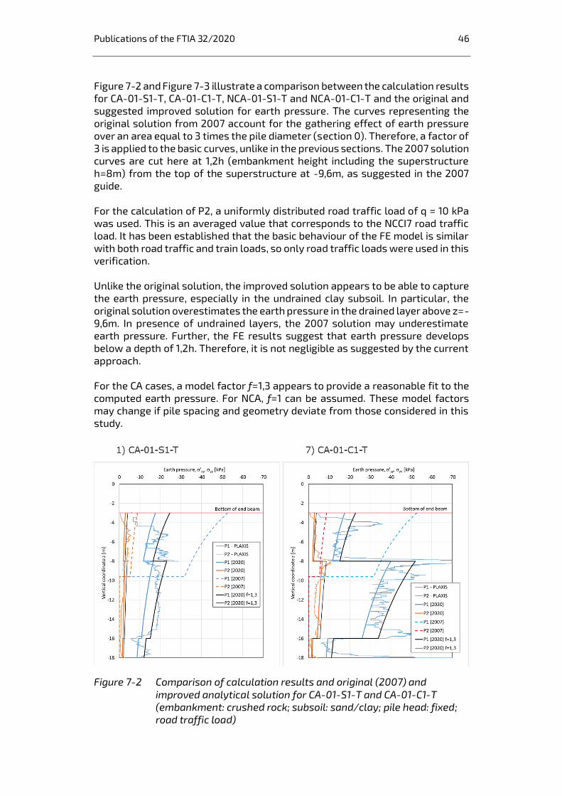
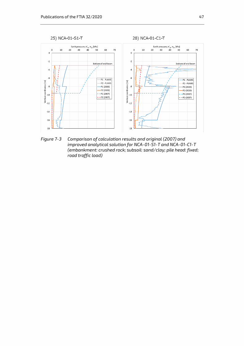
Figure 7-2 and Figure 7-3 illustrate a comparison between the calculation results
for CA-01-S1-T, CA-01-C1-T, NCA-01-S1-T and NCA-01-C1-T and the original and
suggested improved solution for earth pressure. The curves representing the
original solution from 2007 account for the gathering effect of earth pressure
over an area equal to 3 times the pile diameter (section 0). Therefore, a factor of
3 is applied to the basic curves, unlike in the previous sections. The 2007 solution
curves are cut here at 1,2h (embankment height including the superstructure
h=8m) from the top of the superstructure at -9,6m, as suggested in the 2007
guide.
For the calculation of P2, a uniformly distributed road traffic load of q = 10 kPa
was used. This is an averaged value that corresponds to the NCCI7 road traffic
load. It has been established that the basic behaviour of the FE model is similar
with both road traffic and train loads, so only road traffic loads were used in this
verification.
Unlike the original solution, the improved solution appears to be able to capture
the earth pressure, especially in the undrained clay subsoil. In particular, the
original solution overestimates the earth pressure in the drained layer above z=-
9,6m. In presence of undrained layers, the 2007 solution may underestimate
earth pressure. Further, the FE results suggest that earth pressure develops
below a depth of 1,2h. Therefore, it is not negligible as suggested by the current
approach.
For the CA cases, a model factor f=1,3 appears to provide a reasonable fit to the
computed earth pressure. For NCA, f=1 can be assumed. These model factors
may change if pile spacing and geometry deviate from those considered in this
study.
Figure 7-2 Comparison of calculation results and original (2007) and
improved analytical solution for CA-01-S1-T and CA-01-C1-T
(embankment: crushed rock; subsoil: sand/clay; pile head: fixed;
road traffic load)
Publications of the FTIA 32/2020 47
Figure 7-3 Comparison of calculation results and original (2007) and
improved analytical solution for NCA-01-S1-T and NCA-01-C1-T
(embankment: crushed rock; subsoil: sand/clay; pile head: fixed;
road traffic load)

Publications of the FTIA 32/2020 48
8 Discussion
8.1 Using the results of this study when
modelling a pile slab
In presence of a pile slab, the embankment and superstructure are expected to
develop smaller deformations than those observed in this study. Under these
conditions, the mobilized earth pressure may be close to a Ko condition. As the
pile slab supports the superstructure and traffic load, only little earth pressure
loading is expected to act on the bridge piles below the slab. No attempt to
estimate such earth pressure values can be made here.
8.2 Limitations of this study
This study provided insights into the modelling of earth pressure on bridge
abutment piles and compared a 3D numerical to a simple analytical solution.
Nevertheless, the use of FE results needs thoughtful judgment, given the
following limitations:
The results are valid for the geometries and conditions analysed. Results may
differ when pile spacing, pile diameter, abutment geometry, thickness of the
different layers, position of ground water table and construction phases
deviate from the assumptions made in this study.
The earth pressure on piles is modelled from the normal stress acting on a
surface normal to the principal deformation direction of the pile. A full
integration of the stresses acting on the soil-pile interface may provide with
more accurate results. Nevertheless, Ramboll’s experience suggests that the
computed average earth pressures should not deviate significantly from
those obtainable from more advanced integration methods.
Piles are modelled as linear elastic and, therefore, possible yielding cannot be
captured by the model. However, correctly designed piled foundations are not
loaded close to yielding in any case.
Input parameters were determined as “best estimate” parameters based on
literature and experience. No sensitivity study was performed to evaluate the
effect of the single parameters on the numerical results. In general, a proper
parameter assessment would require a comprehensive testing (laboratory/
in-situ) campaign to characterize the different soil units involved in the soil-
structure interaction problem. Further, low and high boundaries of soil
properties should be selected accordingly with the design requirements and
codes.
The clay subsoil is modelled assuming an isotropic undrained shear strength
(su) and a constant shear modulus that is independent of the shear
mobilization in the soil. These assumptions are not realistic (they may be
under specific circumstances), as both su and stiffness of Finnish clays are
known to be stress-path dependent (or anisotropic) (e.g. Lehtonen 2015;

Publications of the FTIA 32/2020 49
Mansikkamäki 2015; D’Ignazio 2016). Further, assuming a constant su may not
reflect the stress state and over-consolidation throughout the model domain.
In presence of clay subsoil, it is crucial to model the correct construction
stages of the embankment and superstructure, including possible preloading
phases. This will provide accurate modelling of shear mobilization in both
coarse and clay layers. In this study, it is assumed that the embankment is
built on the virgin soil prior to the application of the superstructure and the
loads, simulating a long-term condition. While the response under the
external traffic/train loads is substantially undrained, drainage and
consolidation are expected to occur during the construction phases of the
superstructure. Therefore, the computed earth pressure resulting from the
superstructure load (P1) should be intended as the upper boundary
associated with the given set of parameters.
Publications of the FTIA 32/2020 50
9 Summary, conclusions and
recommendations for future research work
9.1 Summary and conclusions
This study focused on modelling earth pressure from traffic and train loads on
abutment piles of integral bridges. Two different bridge abutment
configurations have been analysed: bridge with cantilever span (CA) and bridge
without cantilever span (NCA). The main scope of the study was to compare the
analytical solution from Tiehallinto (2007), which is used in bridge geotechnics
in Finland, with the earth pressure computed from 3D Finite Element analyses
using the Bentley Plaxis 3D program.
The 2007 analytical solution gives the earth pressure based on the earth
pressure coefficient at rest (Ko) and the weight of the embankment/super-
structure material located above the pile heads, assuming a 2:1 stress
distribution with depth. Further, the solution assumes that the earth pressure is
gathered from a 3-pile-diameter width, meaning that the analytical curves
should be multiplied by a factor of three, and that the earth pressure is negligible
below a certain depth according to the thickness of the embankment and
superstructure.
The scope of the FE analyses was to study the effect of using different bridge
configurations, different embankment materials and slope geometries, subsoils
(clay, soft vs sand, stiff) and pile bearings (fully fixed vs free pile head) on the
earth pressure under traffic and train loads.
Coarse (drained) layers were modelled with the Hardening Soil model, which
uses a stress-dependent stiffness and can model hardening along with plastic
straining. The Mohr-Coulomb model with a given undrained shear strength and
a constant shear stiffness was used for the undrained clay subsoil. Piles were
modelled as volume elements with linear elastic behaviour, with interface
elements that ensure strength reduction at the soil-pile interface compared to
the surrounding soil.
Ramboll selected appropriate models and input parameters based on
recommendations from Väylä, available literature and in-house experience. The
parameters are meant to represent a best estimate of the soil properties.
Therefore, the modelled earth pressures are also intended to represent best
estimates.
Results show that in most cases the 2007 analytical solution appears to deviate
from the FE results. The discrepancies are mainly evident in undrained
conditions, where the analytical solution notably underestimates the earth
pressure. The analytical solution seems to agree with the numerical results
when the model behaviour is governed by drained conditions (i.e. with stiff sand
subsoil). Nevertheless, this could be anticipated given its formulation. It must be
pointed out that the analytical curves were not multiplied by a factor of 3 to
account for the stress gathering effect behind the piles. This would have led to
a severe overestimation of earth pressure, especially in the coarse layers. In the

Publications of the FTIA 32/2020 51
FE results, such a “gathering effect” for earth pressure was not visible. More-
over, earth pressure appears to develop over the entire pile length, in contrast
with the recommendations given in previous guidelines.
In general, the Tiehallinto (2007) analytical solution (when including the factor
of 3 and the depth cut-off) seems to:
- overestimate the earth pressure increment in drained conditions,
- underestimate the earth pressure increment in undrained conditions, and
- fully underestimate the earth pressure below a depth of 1,2 times
embankment height
In undrained conditions, the two solutions diverge even in the drained layers,
especially for the NCA cases with clay subsoil. This may be explained by the high
shear mobilization in the embankment that results from the simulation of long-
term conditions (large settlement after construction). The embankment and
superstructure show a softer behaviour compared to the case with stiff (sand)
subsoil, with consequent stress concentration behind the rigid piles. This
behaviour seems to be less pronounced in the CA model with fixed pile-head,
while it tends to disappear when the pile head is free to move (no bearing).
However, the comparison between CA and NCA is not straightforward, given the
differences in the geometry, especially in terms of distance between the piles
and the abutment rigid wall and location of the pile head fixity.
Finally, a way to improve the current analytical solution was proposed based on
the FE results. The improved solution accounts for the Ko of the different soil
layers and it assumes Ko = 1 in undrained conditions. The latter is in line with
basic earth pressure theory. Compared to the standard solution, the improved
solution appears to be able to capture the earth pressure in the undrained layers.
For the drained layers, the benefit is less evident, as some discrepancy remains
between the analytical and the numerical results. In order to obtain a better fit
to the computed earth pressure, model factors are proposed for CA and NCA to.
For CA, the calculated earth pressure needed to be multiplied by a factor of 1,3;
while for NCA this factor could be taken equal to 1. Therefore, the multiplying
factor of 3 recommended in Tiehallinto (2007) appears to be conservative when
applied along with the improved solution. Further, the earth pressure seems to
develop over the entire pile length. Note that these conclusions and proposed
model factors are only valid for the pile spacing, geometry and construction
phases adopted in this study.
9.2 Recommendations for future research
work
It would be of valuable importance in future research to:
Evaluate the effects of geometry, including pile spacing, pile diameter and
thickness of the soil units on the calculated earth pressure.
Evaluate the effect of different construction phases; i.e. evaluating the effect
of constructing the embankment and superstructure before or after pile
installation; evaluating the effect of preload and consolidation in presence of
clay subsoil.
Publications of the FTIA 32/2020 52
Evaluate the effect of forces acting on piles (axial, horizontal and bending)
caused by bridge superstructure and loading.
Evaluate the effect of soil parameters on the model behaviour and perform a
parametric study to evaluate the impact of each model parameter on the
earth pressure. Possibly, include small strain behaviour for both coarse and
fine-grained layers.
Use advanced soil models for clay to model strength and stiffness anisotropy,
shear mobilization and change of anisotropy in the soil. For instance, the
SHANSEP-NGI-ADP model (Panagoulias et al. 2018) or the effective stress
based SCLAY1 or SCLAY-1S model (Karstunen et al. 2005). These models would
require a proper laboratory calibration, even though literature exists on their
use in Finnish soil conditions (e.g. Mansikkamäki 2015; D’Ignazio 2016). When
using advanced models, it is crucial to associate a detailed modelling of all
the construction phases of the embankment and superstructure over the clay
layer(s) (i.e. preloading and consolidation). The models will then predict
undrained behaviour based on the current stress state and shear mobilization
in the soil.
Study the effect of using different FE models on earth pressure. For instance,
compare the Hardening Soil (HS) with Hardening Soil with small strain
(HSsmall) and Mohr-Coulomb with the clay models mentioned above.
If available, back-calculate monitoring data from existing structures to
validate the model’s performance.
Publications of the FTIA 32/2020 53
References
D'Ignazio, M. (2016). Undrained shear strength of Finnish clays for stability
analyses of embankments. PhD thesis, Tampere University of Technology,
Tampere. Publication 1412
Janbu, N. (1998). Sediment deformations. University of Trondheim, Norwegian
University of Science and Technology, Geotechnical Institution. Bulletin, 35, 86.
Karstunen, M., Krenn, H., Wheeler, S. J., Koskinen, M., & Zentar, R. (2005). Effect
of anisotropy and destructuration on the behavior of Murro test embankment.
International Journal of Geomechanics, 5(2), 87-97.
Lehtonen, V. (2015). Modelling undrained shear strength and pore pressure
based on an effective stress soil model in limit equilibrium method. PhD thesis,
Tampere University of Technology, Tampere. Publication 1337.
Liikennevirasto (2017). Eurokoodin soveltamisohje – Geotekninen suunnittelu –
NCCI 7. Siltojen ja pohjarakenteiden suunnitteluohjeet 21.4.2017. Liikenne-
viraston ohjeita 13/2017.
Liikennevirasto (2018). RATO 3. Ratatekniset ohjeet (RATO) osa 3, radan rakenne.
Liikenneviraston ohjeita 13/2018.
Mansikkamäki, J. (2015). Effective stress finite element stability analysis of an
old railway embankment on soft clay. PhD thesis, Tampere University of
Technology, Tampere. Publication 1287.
Panagoulias, S., Vilhar, G., Brinkgreve, R. B. J. (2018) The SHANSEP NGI-ADP model
2018. Plaxis B.V., The Netherlands.
PLAXIS (2020). Bentley Plaxis user’s manual (www.plaxis.nl)
Termaat, R.J., Vermeer, P.A., Vergeer, C.J.H. (1985). Failure by large plastic
deformations. In Proceedings of the 11th International Conference on Soil
Mechanics and Foundation Engineering, San Francisco, 12-16 Aug
Tiehallinto (2007). Sillan geotekniset suunnitteluperusteet. Suunnitteluvaiheen
ohjaus. Tiehallinto, Helsinki.
Väylä (2020). Liikuntasaumattoman sillan suunnittelu, Väyläviraston ohjeita
X/2020 (Draft version/early 2020)

ISSN 2490-0745 ISBN 978-952-317-785-7 www.vayla.fi