FINITE ELEMENT MODELING, COMPUTER SIMULATIONS, AND ...
54
i FINITE ELEMENT MODELING, COMPUTER SIMULATIONS, AND EXPERIMENTS OF SHEAR WAVE PROPAGATION FOR TISSUE MECHANICAL PROPERTY ASSESSMENT By Allison Pinosky Senior Honors Thesis Department of Biomedical Engineering University of North Carolina at Chapel Hill 2015 Approved: ___________________________ Caterina Gallippi, Thesis Advisor Devin Hubbard, Reader Gianmarco Pinton, Reader
Transcript of FINITE ELEMENT MODELING, COMPUTER SIMULATIONS, AND ...

i
FINITE ELEMENT MODELING, COMPUTER SIMULATIONS, AND EXPERIMENTS OF
SHEAR WAVE PROPAGATION FOR TISSUE MECHANICAL PROPERTY ASSESSMENT
By
Allison Pinosky
Senior Honors Thesis
Department of Biomedical Engineering
University of North Carolina at Chapel Hill
2015
Approved:
___________________________
Caterina Gallippi, Thesis Advisor
Devin Hubbard, Reader
Gianmarco Pinton, Reader

ii
© 2015
Allison Pinosky
ALL RIGHTS RESERVED

iii
ABSTRACT
Allison Pinosky: Finite Element Modeling, Computer Simulations, and Experiments of Shear
Wave Propagation for Tissue Mechanical Property Assessment
(Under the direction of Caterina Gallippi)
The goal of this project is to develop a novel approach to tissue mechanical property
measurement using Acoustic Radiation Force Ultrasound. This project aims to do so by
incorporating the quantitative nature of shear wave imaging with the minimal lateral
displacement requirement of acoustic radiation force impulse imaging to develop a novel
approach to tissue mechanical property measurement using statistical signal separation
techniques. By applying a wide tracking beam to a narrow push, it hypothesized that principal
component analysis may be used to reconstruct the shear wave and get tissue mechanical
property information. This new approach will not require spatial averaging, as alternative
methods do, and will therefore better reflect the mechanical properties of heterogeneous tissues.

iv
To Mom, Dad, and Seth, thank you for all of your support.

v
ACKNOWLEDGEMENTS
First and foremost, I would like to thank Dr. Gallippi for the opportunity to conduct
research in her lab and complete this honors thesis. I would also like to thank Tomek
Czernuszewicz for all the time you spent helping me with this project and teaching me about
ultrasound. This project was supported by the Sarah Steele Danhoff Undergraduate Research
Fund administered by Honors Carolina.
vi
TABLE OF CONTENTS
LIST OF TABLES ....................................................................................................................... viii
LIST OF FIGURES ....................................................................................................................... ix
LIST OF ABBREVIATIONS ......................................................................................................... x
LIST OF SYMBOLS ..................................................................................................................... xi
CHAPTER 1: INTRODUCTION TO ULTRASOUND................................................................. 2
Ultrasound Elastography........................................................................................................ 2
Acoustic Radiation Force (ARF) ........................................................................................... 3
ARF Shear Wave Velocity Measurement .............................................................................. 4
Current Methods for Measuring Elasticity ............................................................................ 5
Benefits of Alternative Approach .......................................................................................... 7
CHAPTER 2: BLIND SOURCE SEPARATION (BSS) ............................................................... 8
CHAPTER 3: METHODS ............................................................................................................ 10
Finite Element Method (FEM) Simulation of Tissue Displacement ................................... 10
Simulation of Ultrasonic Displacement Tracking ............................................................... 11
Principal Component Analysis (PCA) Processing of Tracked Data.................................... 12
CHAPTER 4: RESULTS .............................................................................................................. 14
Finite Element Model (FEM) Mesh .................................................................................... 14
Kernels ................................................................................................................................. 15

vii
Velocity Computation .......................................................................................................... 20
CHAPTER 5: CONCLUSION & FUTURE DIRECTION .......................................................... 27
APPENDIX 1: SUPPLEMENTARY MATLAB FIGURES FOR ENTIRE DATA SET ............ 29
APPENDIX 2: SUPPLEMENTARY MATLAB FIGURES FOR KERNELS ............................ 32
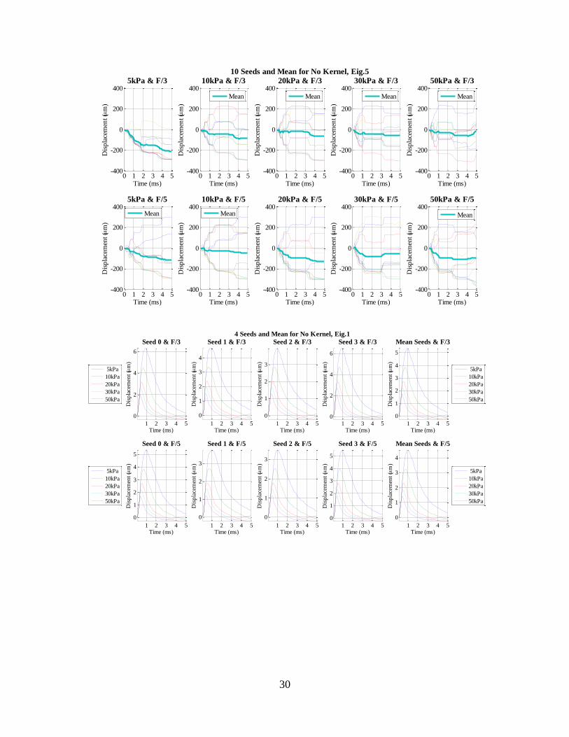
1λ Figures ............................................................................................................................ 32
1.5λ Figures ......................................................................................................................... 34
3λ Figures ............................................................................................................................ 37
Time-to-Peak (TTP) ............................................................................................................. 39
Time-to-Recovery (TTR) ..................................................................................................... 40
REFERENCES ............................................................................................................................. 42
viii
LIST OF TABLES
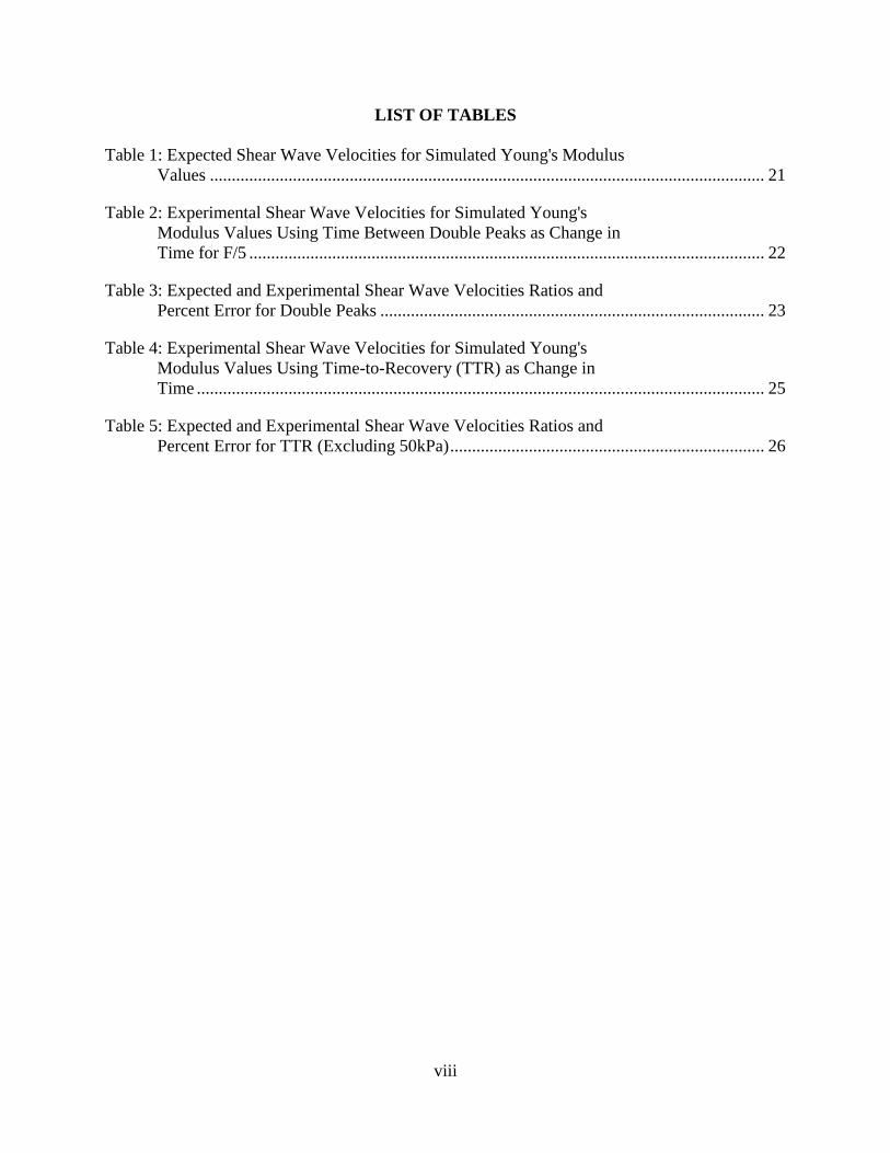
Table 1: Expected Shear Wave Velocities for Simulated Young's Modulus
Values ............................................................................................................................... 21
Table 2: Experimental Shear Wave Velocities for Simulated Young's
Modulus Values Using Time Between Double Peaks as Change in
Time for F/5 ...................................................................................................................... 22
Table 3: Expected and Experimental Shear Wave Velocities Ratios and
Percent Error for Double Peaks ........................................................................................ 23
Table 4: Experimental Shear Wave Velocities for Simulated Young's
Modulus Values Using Time-to-Recovery (TTR) as Change in
Time .................................................................................................................................. 25
Table 5: Expected and Experimental Shear Wave Velocities Ratios and
Percent Error for TTR (Excluding 50kPa) ........................................................................ 26
ix
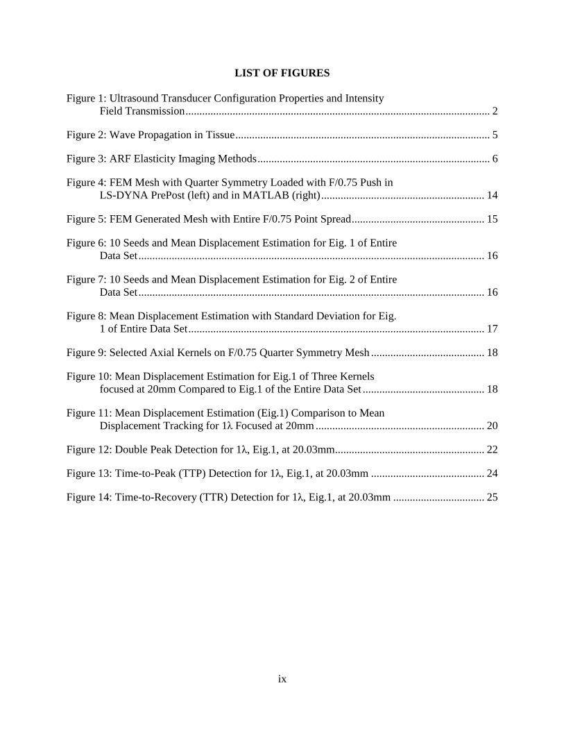
LIST OF FIGURES
Figure 1: Ultrasound Transducer Configuration Properties and Intensity
Field Transmission .............................................................................................................. 2
Figure 2: Wave Propagation in Tissue ............................................................................................ 5
Figure 3: ARF Elasticity Imaging Methods .................................................................................... 6
Figure 4: FEM Mesh with Quarter Symmetry Loaded with F/0.75 Push in
LS-DYNA PrePost (left) and in MATLAB (right) ........................................................... 14
Figure 5: FEM Generated Mesh with Entire F/0.75 Point Spread ................................................ 15
Figure 6: 10 Seeds and Mean Displacement Estimation for Eig. 1 of Entire
Data Set ............................................................................................................................. 16
Figure 7: 10 Seeds and Mean Displacement Estimation for Eig. 2 of Entire
Data Set ............................................................................................................................. 16
Figure 8: Mean Displacement Estimation with Standard Deviation for Eig.
1 of Entire Data Set ........................................................................................................... 17
Figure 9: Selected Axial Kernels on F/0.75 Quarter Symmetry Mesh ......................................... 18
Figure 10: Mean Displacement Estimation for Eig.1 of Three Kernels
focused at 20mm Compared to Eig.1 of the Entire Data Set ............................................ 18
Figure 11: Mean Displacement Estimation (Eig.1) Comparison to Mean
Displacement Tracking for 1λ Focused at 20mm ............................................................. 20
Figure 12: Double Peak Detection for 1λ, Eig.1, at 20.03mm ...................................................... 22
Figure 13: Time-to-Peak (TTP) Detection for 1λ, Eig.1, at 20.03mm ......................................... 24
Figure 14: Time-to-Recovery (TTR) Detection for 1λ, Eig.1, at 20.03mm ................................. 25

x
LIST OF ABBREVIATIONS
ARF Acoustic Radiation Force
BSS Blind Source Separation
FEM Finite Element Method
ICA Independent Component Analysis
PCA Principal Component Analysis
RF Radio-Frequency
ROE Region of Excitation
SNR Signal-to-Noise Ratio
TOF Time-of-Flight
TTP Time-to-Peak
TTR Time-to-Recovery

xi
LIST OF SYMBOLS
α Tissue Attenuation Coefficient
c Speed of Sound
ct Shear Wave Propagation Speed
D Active Aperture Width
E Young’s Modulus
F/# Focal Configuration, F-Number
fS Sampling Frequency
fTX Transmit Frequency
I Local Temporal Average Intensity
λ Wavelength
µ Shear Modulus
ρ Density
ν Poisson Ratio
z Acoustic Focal Depth
2
CHAPTER 1: INTRODUCTION TO ULTRASOUND
Ultrasound imaging uses the transmission of sound and the reception of reflective sound
to construct an image. This is possible because sound is a waveform whose speed depends on the
medium through which it is traveling. Ultrasound provides a non-invasive means of examining
tissue. To observe tissues, sound is transmitted directly into the body using a transducer. The
transducer is capable of both transmitting and receiving acoustic waveforms.
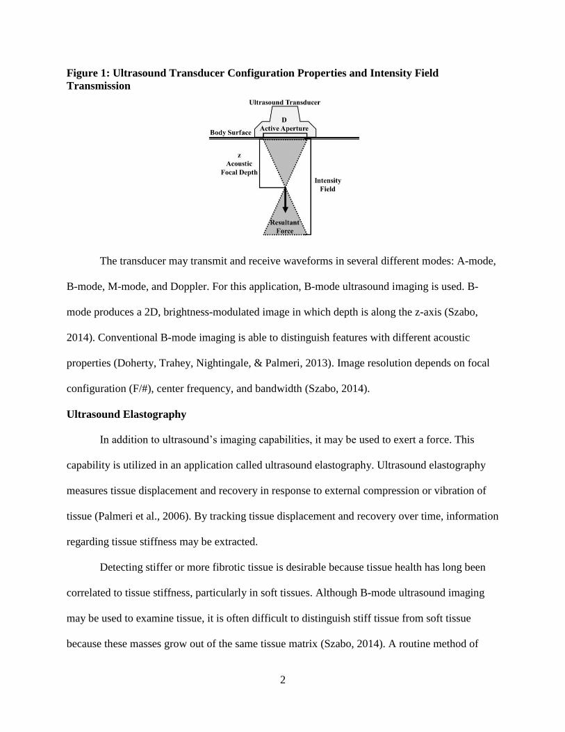
Transducers are made with a variety of geometries and are designed with specific center
frequencies and bandwidths. The transducer of interest for this application is a one-dimensional
(1D) linear array. Linear array transducers are comprised of a single line of elements and have a
fixed elevational focus (Palmeri, McAleavey, Trahey, & Nightingale, 200s6; Szabo, 2014).
Selectively activating elements of this array, allows the creation of narrow or wide beam
apertures. The number of active elements is determined by the beam width and the desired focal
depth. The focal configuration constant, f-number (F/#) is calculated based on the acoustic focal
depth (z) and the active aperture length (D):
𝐹/# =𝑧
𝐷
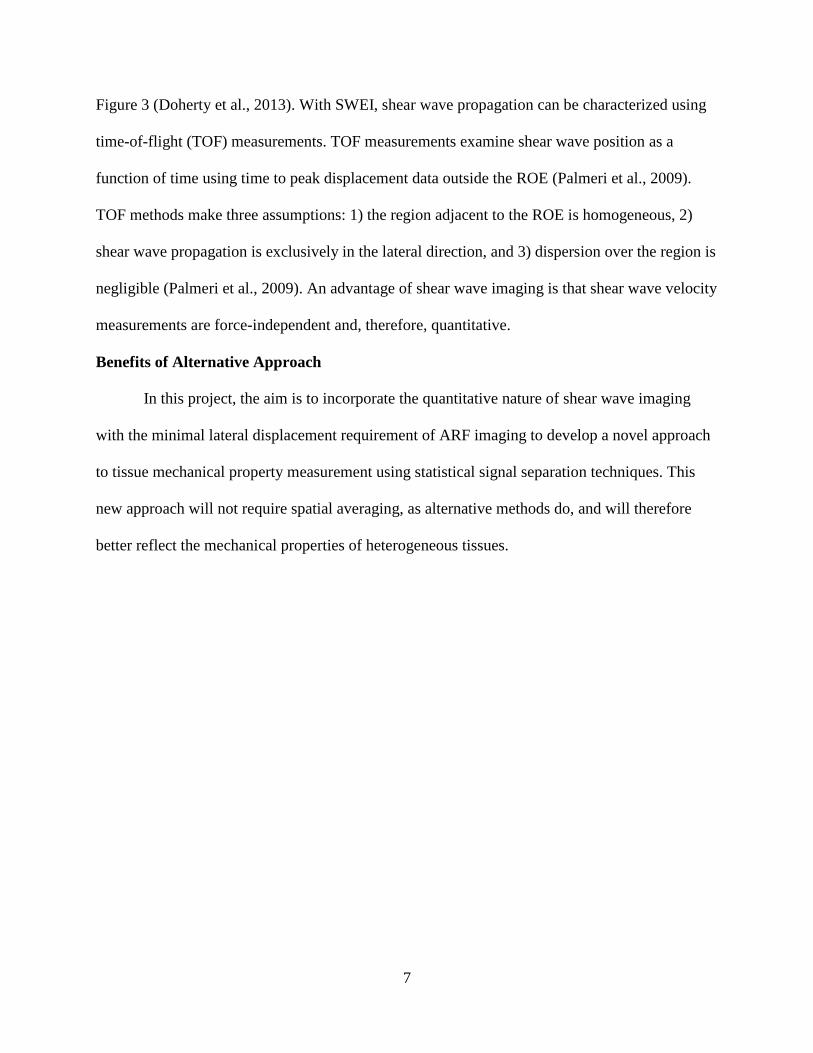
(Palmeri, Wang, Dahl, Frinkley, & Nightengale, 2009). Figure 1 illustrates these parameters.
2
Figure 1: Ultrasound Transducer Configuration Properties and Intensity Field
Transmission
The transducer may transmit and receive waveforms in several different modes: A-mode,
B-mode, M-mode, and Doppler. For this application, B-mode ultrasound imaging is used. B-
mode produces a 2D, brightness-modulated image in which depth is along the z-axis (Szabo,
2014). Conventional B-mode imaging is able to distinguish features with different acoustic
properties (Doherty, Trahey, Nightingale, & Palmeri, 2013). Image resolution depends on focal
configuration (F/#), center frequency, and bandwidth (Szabo, 2014).
Ultrasound Elastography
In addition to ultrasound’s imaging capabilities, it may be used to exert a force. This
capability is utilized in an application called ultrasound elastography. Ultrasound elastography
measures tissue displacement and recovery in response to external compression or vibration of
tissue (Palmeri et al., 2006). By tracking tissue displacement and recovery over time, information
regarding tissue stiffness may be extracted.
Detecting stiffer or more fibrotic tissue is desirable because tissue health has long been
correlated to tissue stiffness, particularly in soft tissues. Although B-mode ultrasound imaging
may be used to examine tissue, it is often difficult to distinguish stiff tissue from soft tissue
because these masses grow out of the same tissue matrix (Szabo, 2014). A routine method of

3
detecting superficial stiff regions is used to detect cancerous legions in breast tissue. By
manually pressing on the superficial tissue, it is possible to physically feel discontinuities in the
tissue (Doherty et al., 2013). These discontinuities, or stiff regions, may constitute cancerous
legions. This manual palpation procedure may be replicated at locations deeper in the tissue via
ultrasound elastography.
To understand how ultrasound elastography works in tissue, a base understanding of
material elasticity must be established. Material elasticity describes the tendency of the material
to deform in response to an applied force (Doherty et al., 2013). Material stiffness may described
by Young’s modulus. Young’s modulus (E) may be calculated in terms of shear wave modulus
(µ) and Poisson Ratio (v):
𝐸 = 𝜇 ∗ 2(1 + 𝑣) .
Shear modulus describes a material’s resistance to shear while Poisson’s ratio describes the
deformation that occurs orthogonal to the material (Doherty et al., 2013).
Acoustic Radiation Force (ARF)
One method of conducting ultrasound elastography is by exciting the tissue with acoustic
radiation force (ARF) (Palmeri et al., 2006). ARF employs a multi-cycle ultrasonic pulse that
generates a force in the propagation medium using a single transducer. The force applied by
conventional ultrasound imaging is not substantial enough to produce measureable displacements
(Doherty et al., 2013). To create tissue displacements in the range of 1 to 10µm, peak ARF
magnitudes are typically on the order of dynes (Doherty et al., 2013). The magnitude of localized
compression in response to ARF is inversely correlated to the underlying stiffness (Nightingale,
2012). Therefore, softer tissues will displace further than stiff tissues.
4
ARF induces the propagation of acoustic waves through dissipative medium (Fahey,
Nightingale, Nelson, Palmeri, & Trahey, 2005). In soft tissue, the majority of attenuation of an
acoustic wave is due to absorption. The radiation force applied to tissue at any given spatial
location may be calculated in terms of tissue attenuation coefficient (α), local temporal average
intensity (I), and the speed of sound in tissue (c):
𝐹 =2∝𝐼
𝑐 ,
(Mazza, Nava, Hahnloser, Jochum, & Bajka, 2007; Nightingale, 2012). The resultant radiation
force is localized in the center of the intensity field laterally and at the acoustic focal point
axially. The shape of the intensity field, depicted in Figure 1, is dependent upon F/# (Palmeri et
al., 2009).
Initially, tissue displacement response to the ARF is restricted to the region of excitation
(ROE), with the peak displacements occurring near the acoustic focal location. Standard B-mode
pulses may be used to monitor the movement of tissue under force. Behavior of the tissue
following the initial excitation will be addressed in the following section.
ARF Shear Wave Velocity Measurement
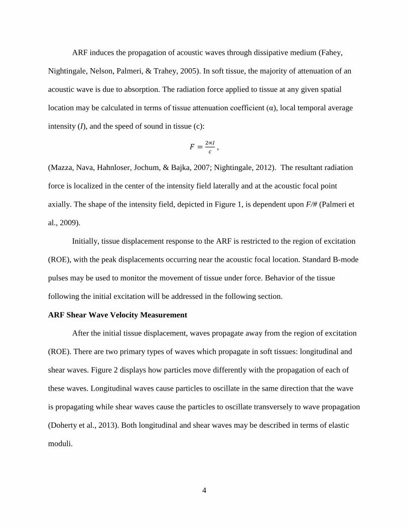
After the initial tissue displacement, waves propagate away from the region of excitation
(ROE). There are two primary types of waves which propagate in soft tissues: longitudinal and
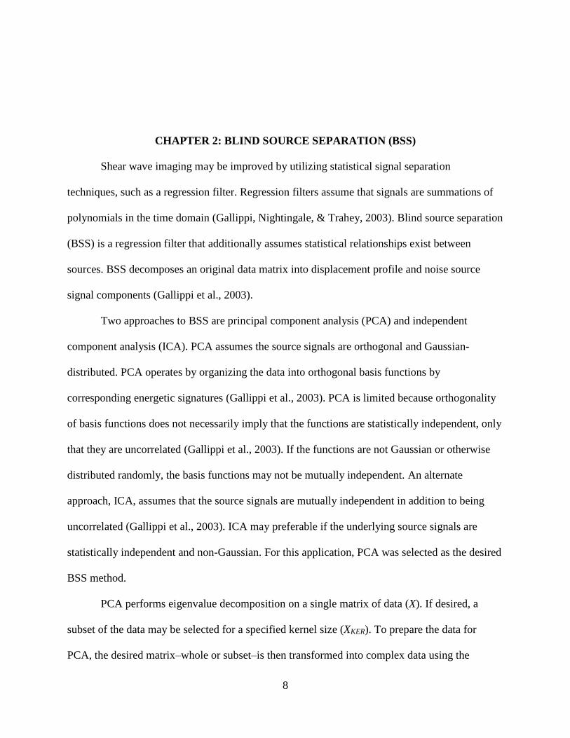
shear waves. Figure 2 displays how particles move differently with the propagation of each of
these waves. Longitudinal waves cause particles to oscillate in the same direction that the wave
is propagating while shear waves cause the particles to oscillate transversely to wave propagation
(Doherty et al., 2013). Both longitudinal and shear waves may be described in terms of elastic
moduli.
5
Figure 2: Wave Propagation in Tissue
(Figure adapted from Olympus Corporation, n.d.)
In response to the ARF impulse, shear waves propagate radially away from the ROE.
Tissue stiffness may then be inferred by measuring the velocity of the propagating shear wave. A
faster shear wave velocity indicates propagation through stiffer tissue. This shear wave velocity
(ct), may be described in terms of shear modulus (µ) and in terms of tissue density (ρ):
𝑐𝑡 = √µ
𝜌
(Nightingale, 2012). Because shear modulus may be described in terms of Young’s Modulus
(E), shear wave velocity may be directly related to the Young’s modulus of the tissue without
requiring information about the force magnitude:
𝑐𝑡 = √𝐸
2(1 + 𝑣)𝜌 .
Current Methods for Measuring Elasticity
ARF methods are classified by the type of excitation pulse applied and the position of the
tracking beams relative to the region of excitation (ROE). One excitation method, discussed
herein, applies pulses—pushes—transiently in an impulse-like fashion (Doherty et al., 2013).
6
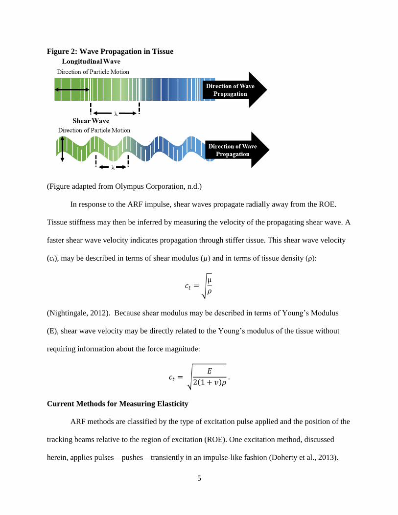
The tracking beam can then be placed on-axis (within the ROE) or off-axis (outside the ROE).
Generally, on-axis methods can only provide relative, qualitative measures of elasticity while
off-axis methods provide quantitative estimates (Doherty et al., 2013).
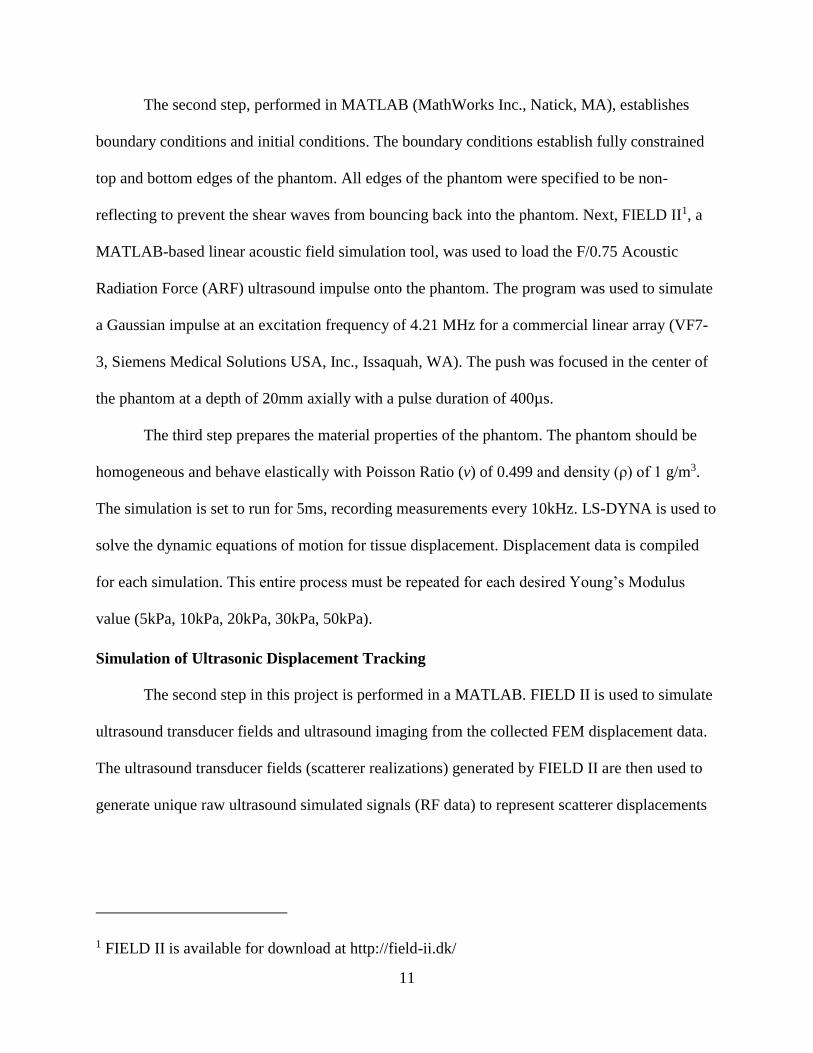
On-axis tracking may be performed using Acoustic Radiation Force Impulse (ARFI)
imaging. ARFI excites and tracks tissue response from a single location (Figure 3). Then, the
active aperture on the transducer is shifted over by one element, and the push and track sequence
is repeated (Doherty et al., 2013). This process is repeated laterally across the field of view. The
ARF induced compression is tracked with by B-mode pulses, which are used to detect the
displacement of tissue and observe the recovery rate to the original state. ARFI images taken
represent mechanical properties of the tissue rather than the acoustic properties. Axial
displacements can then be calculated with normalized cross-correlation methods or phase-shift
algorithms (Doherty et al., 2013). ARF allows relativistic detection of structural components but
is unable to quantify the stiffness of structures absolutely because the true magnitude of the
displacing force is unknown.
Figure 3: ARF Elasticity Imaging Methods
(Figure adapted from Doherty et al., 2013)
Off-axis tracking may be performed with Shear Wave Elasticity Imaging (SWEI). SWEI
is an ARF method that tracks induced shear waves that radiate outward from the region of
excitation. For SWEI, a push is emitted at one location and then the shear wave is tracked at
multiple off-axis lateral locations at known distances from the initial push, as may be seen in
7
Figure 3 (Doherty et al., 2013). With SWEI, shear wave propagation can be characterized using
time-of-flight (TOF) measurements. TOF measurements examine shear wave position as a
function of time using time to peak displacement data outside the ROE (Palmeri et al., 2009).
TOF methods make three assumptions: 1) the region adjacent to the ROE is homogeneous, 2)
shear wave propagation is exclusively in the lateral direction, and 3) dispersion over the region is
negligible (Palmeri et al., 2009). An advantage of shear wave imaging is that shear wave velocity
measurements are force-independent and, therefore, quantitative.
Benefits of Alternative Approach
In this project, the aim is to incorporate the quantitative nature of shear wave imaging
with the minimal lateral displacement requirement of ARF imaging to develop a novel approach
to tissue mechanical property measurement using statistical signal separation techniques. This
new approach will not require spatial averaging, as alternative methods do, and will therefore
better reflect the mechanical properties of heterogeneous tissues.
8
CHAPTER 2: BLIND SOURCE SEPARATION (BSS)
Shear wave imaging may be improved by utilizing statistical signal separation
techniques, such as a regression filter. Regression filters assume that signals are summations of
polynomials in the time domain (Gallippi, Nightingale, & Trahey, 2003). Blind source separation
(BSS) is a regression filter that additionally assumes statistical relationships exist between
sources. BSS decomposes an original data matrix into displacement profile and noise source
signal components (Gallippi et al., 2003).
Two approaches to BSS are principal component analysis (PCA) and independent
component analysis (ICA). PCA assumes the source signals are orthogonal and Gaussian-
distributed. PCA operates by organizing the data into orthogonal basis functions by
corresponding energetic signatures (Gallippi et al., 2003). PCA is limited because orthogonality
of basis functions does not necessarily imply that the functions are statistically independent, only
that they are uncorrelated (Gallippi et al., 2003). If the functions are not Gaussian or otherwise
distributed randomly, the basis functions may not be mutually independent. An alternate
approach, ICA, assumes that the source signals are mutually independent in addition to being
uncorrelated (Gallippi et al., 2003). ICA may preferable if the underlying source signals are
statistically independent and non-Gaussian. For this application, PCA was selected as the desired
BSS method.
PCA performs eigenvalue decomposition on a single matrix of data (X). If desired, a
subset of the data may be selected for a specified kernel size (XKER). To prepare the data for
PCA, the desired matrix–whole or subset–is then transformed into complex data using the

9
Hilbert transform (XH). This transformation is necessary because the purpose of performing PCA
in this application is to attempt to isolate the shear wave propagating through the medium. Using
complex data allows the decomposition to encode directional information.
Prior to eigenvalue decomposition, the data must be mean centered. This is accomplished
by taking the mean of the data at each time point and subtracting that value from each element in
the vector for the respective time point, resulting in a mean-centered matrix (XMC). For an [𝑀𝑥𝑁]
matrix XH, where the N-dimension is the time-dimension, the following equation may be used to
mean center the data:
𝑋𝑀𝐶 = [
𝑥1,1 − 𝑥1̅̅̅ ⋯ 𝑥1,𝑁 − 𝑥𝑁̅̅̅̅⋮ ⋱ ⋮
𝑥𝑀,1 − 𝑥1̅̅̅ ⋯ 𝑥𝑀,𝑁 − 𝑥𝑁̅̅̅̅]
where 𝑥𝑛̅̅ ̅ is the mean of respective columns n = 1…N and xi,n represent each element of the
Hilbert transformed matrix (XH) for i = 1…M. Next, the covariance matrix is computed and
normalized:
𝑋𝐶𝑂𝑉 =𝑋𝑀𝐶 ’ ∗ 𝑋𝑀𝐶
𝑁 − 1
where XMC is the mean-centered, Hilbert transformed [𝑀𝑥𝑁] matrix and N is the number of
time points.
Once the covariance matrix is computed, it can be decomposed into orthogonal
eigenvalues and eigenvectors. BSS derived basis functions describe the contribution of the
source signals that they span over time of ensemble acquisition (Gallippi et al., 2003).
The eigenvalues with the larger values correspond to more energetic signals.

10
CHAPTER 3: METHODS
The aim of this project is to develop a method of separating ARFI data using BSS to
allow shear wave tracking over a smaller area than is currently possible. The hope is that this will
reduce inaccuracies due to special averaging. It is hypothesized that in order for BSS to be able
to successfully separate out a shear wave velocity, a large tracking beam width, relative to a
smaller tracking aperture, must be used.
Finite Element Method (FEM) Simulation of Tissue Displacement
Finite Element Method (FEM) is a mathematical way of finding approximate solutions to
complex numerical problems for partial differential equations. For this project, an FEM model
was developed to simulate radiation force-induced shear waves with a tight focal configuration
(F/0.75) in a linearly elastic model. Simulated phantoms are uniform in geometry but differ by
Young’s Modulus values (5kPa, 10kPa, 20kPa, 30kPa, and 50kPa).
The first phantom generation step establishes phantom geometry. The phantoms are
simulated using LS-DYNA’s sub-program LS-PrePost (LS-DYNA, Livermore Software
Technology Corporation, Livermore, CA). This program develops phantoms by generating a
mesh. For each phantom, the fineness of the mesh and the distance in the elevational (x), lateral
(y), and axial (z) directions may be specified. The finer the mesh, the more locations at which
forces may be loaded and calculations performed. The tradeoff is that calculations for finer
meshes take significantly longer to complete. To reduce the time required, phantoms may be
constructed with quarter symmetry. For these simulations, a finely spaced phantom with quarter
symmetry was constructed with dimensions of 10mm x 10mm x 40mm.
11
The second step, performed in MATLAB (MathWorks Inc., Natick, MA), establishes
boundary conditions and initial conditions. The boundary conditions establish fully constrained
top and bottom edges of the phantom. All edges of the phantom were specified to be non-
reflecting to prevent the shear waves from bouncing back into the phantom. Next, FIELD II1, a
MATLAB-based linear acoustic field simulation tool, was used to load the F/0.75 Acoustic
Radiation Force (ARF) ultrasound impulse onto the phantom. The program was used to simulate
a Gaussian impulse at an excitation frequency of 4.21 MHz for a commercial linear array (VF7-
3, Siemens Medical Solutions USA, Inc., Issaquah, WA). The push was focused in the center of
the phantom at a depth of 20mm axially with a pulse duration of 400µs.
The third step prepares the material properties of the phantom. The phantom should be
homogeneous and behave elastically with Poisson Ratio (v) of 0.499 and density (ρ) of 1 g/m3.
The simulation is set to run for 5ms, recording measurements every 10kHz. LS-DYNA is used to
solve the dynamic equations of motion for tissue displacement. Displacement data is compiled
for each simulation. This entire process must be repeated for each desired Young’s Modulus
value (5kPa, 10kPa, 20kPa, 30kPa, 50kPa).
Simulation of Ultrasonic Displacement Tracking
The second step in this project is performed in a MATLAB. FIELD II is used to simulate
ultrasound transducer fields and ultrasound imaging from the collected FEM displacement data.
The ultrasound transducer fields (scatterer realizations) generated by FIELD II are then used to
generate unique raw ultrasound simulated signals (RF data) to represent scatterer displacements
1 FIELD II is available for download at http://field-ii.dk/

12
in tissue. This process is performed for several variations of tracking aperture widths (F/0.75,
F/1.5, F/3.0 and F/5.0).
Typically, the program determines the number of scatterers required based on the F/# for
that specific simulation. To attain comparable results across different F/#’s, the scatterer number
per resolution cell can be set to a uniform value for all simulations. This constraint is acceptable
because it is only necessary for there to be at least 11 scatterers per resolution cell to ensure fully
developed speckle. Furthermore, uniform scatterer number will ensure a signal-to-noise ratio
(SNR) in the desired range. Approximately 1.2 million scatterers are used for these simulations,
ensuring sufficient SNR. By re-running FIELD II for different scatterer realizations (seeds),
multiple trials of RF data may be compiled for each stiffness and F/#.
Principal Component Analysis (PCA) Processing of Tracked Data
The third step in this project performs Principal Component Analysis (PCA) on the
FIELD II simulated RF data. To perform PCA, all simulated RF data—for the desired scatterer
realization, F/#, and Young’s Modulus value—is loaded into a single matrix. Then, subsets of the
data are selected using a specific kernel sizes. Kernel sizes are selected based on the sampling
frequency (fs), 200MHz, and wavelength (λ) of the RF data. The wavelength may be calculated
from the speed of sound in tissue (c) and the transmission frequency (fTX), 6.15MHz:
𝜆 =𝑐
𝑓𝑇𝑋 .
Similarly, the displacement per sample (DispPerSample) may be calculated from the speed of
sound in tissue (c) and the sampling frequency (fS):
𝐷𝑖𝑠𝑝𝑃𝑒𝑟𝑆𝑎𝑚𝑝𝑙𝑒 =𝑐
2 ∗ 𝑓𝑆 .
The displacement per sample must be divided by two to account for the time it takes for the
13
acoustic wave to travel into the tissue and reflect back. The number of samples required for the
kernel (SKER) can then be found for the desired portion of the wavelength (KER):
𝑆𝐾𝐸𝑅 =𝐾𝐸𝑅 ∗ 𝜆
𝐷𝑖𝑠𝑝𝑃𝑒𝑟𝑆𝑎𝑚𝑝𝑙𝑒 .
Note, that subsequent discussions of subsets will define them in terms of wavelength in the form
#λ. The desired matrix–whole or subset–is then transformed into complex data using the Hilbert
transform.
Once the Hilbert transform is performed, the data mean centered, and the covariance
matrix is computed. Then, the covariance matrix is decomposed into eigenvalues and
eigenvectors. For this project, the eigenvectors corresponding to the 5 largest eigenvalues were
of interest. Then, the eigenvectors are converted to displacements. This is accomplished by
taking the unwrapped phase of each eigenvector and subtracting the minimum of each
eigenvector from each element in that eigenvector. Then, each element is multiplied by the
sampling frequency and divided by the estimated center frequency (via the Loupas Method) and
finally multiplied by the displacement per sample to output the PCA estimated displacements
(Mauldin, Viola, & Walsker, 2010).

14
CHAPTER 4: RESULTS
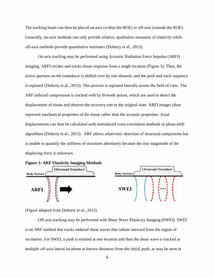
Finite Element Model (FEM) Mesh
Finite element method (FEM) mesh generation resulted in a phantom with quarter
symmetry loaded with an ultrasound impulse with a tight focal configuration (F/0.75). This focal
configuration served as the push for all simulations. Figure 4-left displays the finely spaced mesh
loaded with force corresponding to F/0.75 in LS-DYNA. This spread may be similarly plotted in
MATLAB. Figure 4-right displays the same point loads as the figure on the left, additionally
indicating the location of the acoustic focal depth. The point loads appear to begin around
-13mm rather than extending from the surface of the phantom (0mm). This gap results from
thresh-holding which occurs during point load simulation. In reality, some force would be
present in the region between -13mm and 0mm and would extend below the hourglass shape.
Figure 4: FEM Mesh with Quarter Symmetry Loaded with F/0.75 Push in LS-DYNA
PrePost (left) and in MATLAB (right)
0 2 4 6 8 10
-40
-35
-30
-25
-20
-15
-10
-5
0
Lateral (mm)
Point Loads Location for F/0.75 Tight Configuration
of Phantom Mesh with Quarter Symmetry
Ax
ial
(mm
)
Point Loads
Acoustic Focal Depth

15
The entire push may be simulated in MATLAB by mirroring the single-quadrant point
loads (from Figure 4) over the x and y axes. Figure 5 displays entire F/0.75 points spread
forming the hourglass shape characteristic of ultrasound.
Figure 5: FEM Generated Mesh with Entire F/0.75 Point Spread
Kernels
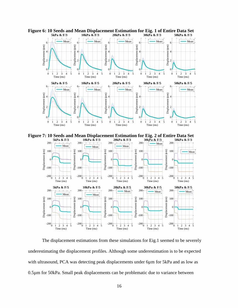
Initially, PCA was performed on the entire simulated ultrasound signal matrix. It was
hypothesized that the estimated displacement profile for the first eigenvalue (Eig.1) would reflect
the initial shear wave, and the second eigenvalue (Eig.2) would show the shear wave later in
time, after it had propagated to the edge of the resolution cell. The estimated displacement
profiles for 10 scatterer realizations as well as the mean of these signals for Eig.1 are displayed
in Figure 6. The signals from Eig.2 are similarly displayed in Figure 7. Subplots increase in
Young’s Modulus value from left to right across the rows and increase in F/# down the columns.
Eig.1 resembles the displacement profile for a shear wave, but Eig.2 does not. At this time, there
is no apparent correlation between shear wave propagation and eigenvectors beyond Eig.1.
Therefore, only Eig.1 will be discussed herein2.
2 Additional figures with the 10 seeds and means for Eig.3, Eig.4 and Eig.5 are located in Appendix 1.
-10-5
05
10 -10 -5 0 5 10
-40
-35
-30
-25
-20
-15
-10
-5
0
Lateral (mm)
Point Loads Location for F/0.75 Tight Configuration of Full Phantom Mesh
Elevational (mm)
Ax
ial
(mm
)
Point Loads
Acoustic Focal Depth
16
Figure 6: 10 Seeds and Mean Displacement Estimation for Eig. 1 of Entire Data Set
Figure 7: 10 Seeds and Mean Displacement Estimation for Eig. 2 of Entire Data Set
The displacement estimations from these simulations for Eig.1 seemed to be severely
underestimating the displacement profiles. Although some underestimation is to be expected
with ultrasound, PCA was detecting peak displacements under 6µm for 5kPa and as low as
0.5µm for 50kPa. Small peak displacements can be problematic due to variance between
0 1 2 3 4 5
0
2
4
6
Time (ms)
Dis
pla
cem
ent
(m
)
5kPa & F/3
Mean
0 1 2 3 4 5
0
2
4
6
Time (ms)
Dis
pla
cem
ent
(m
)
5kPa & F/5
Mean
0 1 2 3 4 5
0
2
4
6
Time (ms)D
isp
lace
men
t (
m)
10kPa & F/3
Mean
0 1 2 3 4 5
0
2
4
6
Time (ms)
Dis
pla
cem
ent
(m
)
10kPa & F/5
Mean
0 1 2 3 4 5
0
2
4
6
Time (ms)
Dis
pla
cem
ent
(m
)
10 Seeds and Mean for No Kernel, Eig.1
20kPa & F/3
Mean
0 1 2 3 4 5
0
2
4
6
Time (ms)
Dis
pla
cem
ent
(m
)
20kPa & F/5
Mean
0 1 2 3 4 5
0
2
4
6
Time (ms)
Dis
pla
cem
ent
(m
)
30kPa & F/3
Mean
0 1 2 3 4 5
0
2
4
6
Time (ms)
Dis
pla
cem
ent
(m
)
30kPa & F/5
Mean
0 1 2 3 4 5
0
2
4
6
Time (ms)
Dis
pla
cem
ent
(m
)
50kPa & F/3
Mean
0 1 2 3 4 5
0
2
4
6
Time (ms)
Dis
pla
cem
ent
(m
)
50kPa & F/5
Mean
0 1 2 3 4 5-200
-100
0
100
200
Time (ms)
Dis
pla
cem
ent
(m
)
5kPa & F/3
Mean
0 1 2 3 4 5-200
-100
0
100
200
Time (ms)
Dis
pla
cem
ent
(m
)
5kPa & F/5
Mean
0 1 2 3 4 5-200
-100
0
100
200
Time (ms)
Dis
pla
cem
ent
(m
)
10kPa & F/3
Mean
0 1 2 3 4 5-200
-100
0
100
200
Time (ms)
Dis
pla
cem
ent
(m
)
10kPa & F/5
Mean
0 1 2 3 4 5-200
-100
0
100
200
Time (ms)
Dis
pla
cem
ent
(m
)
10 Seeds and Mean for No Kernel, Eig.2
20kPa & F/3
Mean
0 1 2 3 4 5-200
-100
0
100
200
Time (ms)
Dis
pla
cem
ent
(m
)
20kPa & F/5
Mean
0 1 2 3 4 5-200
-100
0
100
200
Time (ms)
Dis
pla
cem
ent
(m
)
30kPa & F/3
Mean
0 1 2 3 4 5-200
-100
0
100
200
Time (ms)
Dis
pla
cem
ent
(m
)
30kPa & F/5
Mean
0 1 2 3 4 5-200
-100
0
100
200
Time (ms)
Dis
pla
cem
ent
(m
)
50kPa & F/3
Mean
0 1 2 3 4 5-200
-100
0
100
200
Time (ms)
Dis
pla
cem
ent
(m
)
50kPa & F/5
Mean

17
samples. Figure 8 displays the mean estimated displacement profiles of 10 scatterer realizations
for Eig.1 from PCA on the entire data set. The error bars indicate standard deviation of the 10
seeds from Figure 6 at each time point. For 5kPa, the mean maximum peak displacement is
~5µm, and the standard deviation is ~1.25µm. In this case, the standard deviation is 25% of the
peak displacement.
Figure 8: Mean Displacement Estimation with Standard Deviation for Eig. 1 of Entire Data
Set
To attempt to reduce this underestimation and make the standard deviations less
significant, axial kernels of the data were selected to perform PCA. The process for extracting
these subsets was addressed in the methods chapter. Many normalized cross-correlation methods
use kernels of 1.5λ, so initially, kernel sizes of 1λ, 1.5λ, and 3λ were selected. Kernel location
may also be selected. It was hypothesized that the kernel should be located at the acoustic focal
depth (20mm) because this is the depth at which the acoustic radiation force (ARF) is most
uniform laterally and in magnitude. Therefore, kernel subsets were initially centered at 20mm.
Figure 9 displays the selected axial kernels on the F/0.75 quarter symmetry mesh.
1 2 3 4 5
0
2
4
6
5kPa & F/3
Time (ms)
Dis
pla
cem
ent
(m
)
1 2 3 4 5
0
2
4
65kPa & F/5
Time (ms)
Dis
pla
cem
ent
(m
)
1 2 3 4 5
0
2
4
6
10kPa & F/3
Time (ms)
Dis
pla
cem
ent
(m
)
1 2 3 4 5
0
2
4
610kPa & F/5
Time (ms)
Dis
pla
cem
ent
(m
)
1 2 3 4 5
0
2
4
6
Mean with Standard Deviation of 10 Seeds for No Kernel, Eig.1
20kPa & F/3
Time (ms)
Dis
pla
cem
ent
(m
)
1 2 3 4 5
0
2
4
620kPa & F/5
Time (ms)
Dis
pla
cem
ent
(m
)
1 2 3 4 5
0
2
4
6
30kPa & F/3
Time (ms)D
isp
lace
men
t (
m)
1 2 3 4 5
0
2
4
630kPa & F/5
Time (ms)
Dis
pla
cem
ent
(m
)
1 2 3 4 5
0
2
4
6
50kPa & F/3
Time (ms)
Dis
pla
cem
ent
(m
)
1 2 3 4 5
0
2
4
650kPa & F/5
Time (ms)
Dis
pla
cem
ent
(m
)

18
Figure 9: Selected Axial Kernels on F/0.75 Quarter Symmetry Mesh
Figure 10 displays the mean estimated displacement profiles for Eig.1 for kernels 1λ,
1.5λ, and 3λ plotted on the same figure as the result of PCA on the entire data set. This figure
more clearly shows the underestimation resulting from performing PCA on the entire data set.
Therefore, only kernels of data are examined herein.3
Figure 10: Mean Displacement Estimation for Eig.1 of Three Kernels focused at 20mm
Compared to Eig.1 of the Entire Data Set
3Additional figures with for 1λ, 1.5λ, and 3λ Eig.1 are located in Appendix 2
0 1 2 3 4 5-5
0
5
10
15
20
255kPa & F/3
Time (ms)
Dis
pla
cem
ent
(m
)
0 1 2 3 4 5-5
0
5
10
15
20
255kPa & F/5
Time (ms)
Dis
pla
cem
ent
(m
)
0 1 2 3 4 5-5
0
5
10
15
20
2510kPa & F/3
Time (ms)
Dis
pla
cem
ent
(m
)
0 1 2 3 4 5-5
0
5
10
15
20
2510kPa & F/5
Time (ms)
Dis
pla
cem
ent
(m
)
0 1 2 3 4 5-5
0
5
10
15
20
25
Mean of 10 Seeds, Kernel Comparison to No Kernel, Kernels Focused at 20 mm, Eig.1
20kPa & F/3
Time (ms)
Dis
pla
cem
ent
(m
)
0 1 2 3 4 5-5
0
5
10
15
20
2520kPa & F/5
Time (ms)
Dis
pla
cem
ent
(m
)
0 1 2 3 4 5-5
0
5
10
15
20
2530kPa & F/3
Time (ms)
Dis
pla
cem
ent
(m
)
0 1 2 3 4 5-5
0
5
10
15
20
2530kPa & F/5
Time (ms)
Dis
pla
cem
ent
(m
)
0 1 2 3 4 5-5
0
5
10
15
20
2550kPa & F/3
Time (ms)
Dis
pla
cem
ent
(m
)
0 1 2 3 4 5-5
0
5
10
15
20
2550kPa & F/5
Time (ms)
Dis
pla
cem
ent
(m
)
1
1.5
3
None
1
1.5
3
None
1
1.5
3
None
1
1.5
3
None
1
1.5
3
None
1
1.5
3
None
1
1.5
3
None
1
1.5
3
None
1
1.5
3
None
1
1.5
3
None
0 2 4 6 8 10-40
-35
-30
-25
-20
-15
-10
-5
0
Lateral (mm)
Axia
l (m
m)
Point Loads
Acoustic Focal Depth
0 0.5 1 1.5 2 2.5 3-30
-28
-26
-24
-22
-20
-18
-16
-14
-12
-10
Lateral (mm)
Axia
l (m
m)
Point Loads
Acoustic Focal Depth
1 Kernel
1.5 Kernel
3 Kernel

19
Further examination of the kernels noted that some of the plots were not smooth, but
instead featured double peaks. The peaks seemed to be most apparent in the 1λ kernel with F/5
tracking. Therefore, this case will be the focus of the remaining figures and double peak
detection and analysis. Although the source of this double peak is unknown, the peaks appear to
get closer together in time as stiffness increases. This is also characteristic of shear wave
movement—as the material gets stiffer, shear waves may propagate faster. It was hypothesized
that shear wave movement was in fact not orthogonal. PCA separates eigenvectors by
orthogonality, so if the two cases of shear wave detection were not orthogonal, then they would
not be separated into two different eigenvectors. Therefore, it may be possible that the first peak
is the initially detected shear wave and the second peak is the shear wave which was detected
after it propagated. This suspicion led to an interest in quantifying the change in distance and
time between the peaks via shear wave velocity calculations.
In an attempt to determine the source of the double peaks, displacement tracking was
performed on the generated displacement data. Simulated tracking is performed by a previously
developed script in the lab, ‘createSimResDisp.dat’. This program treats each junction in the
mesh like a scatterer, and tracks its displacement over time. The output allows motion tracking
through time of a specified location—indicated by x, y, z, coordinates.
In this project, PCA is performed on the simulated ultrasound data, so rather than merely
tracking individual nodes, it is more useful to perform averaging. This averaging should be
restricted to the resolution cell. The resolution cell size is dependent upon F/#, kernel size, and
transducer. The F/# of the tracking beam determines the lateral distance spanned by the
resolution cell. The kernel size determines the axial distance spanned by the resolution cell.
Since the transducer used for this application is 1D linear array, the elevational distance of the
20
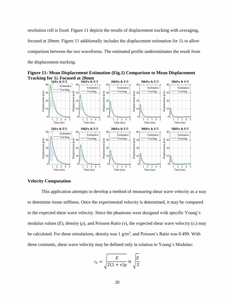
resolution cell is fixed. Figure 11 depicts the results of displacement tracking with averaging,
focused at 20mm. Figure 11 additionally includes the displacement estimation for 1λ to allow
comparison between the two waveforms. The estimated profile underestimates the result from
the displacement tracking.
Figure 11: Mean Displacement Estimation (Eig.1) Comparison to Mean Displacement
Tracking for 1λ Focused at 20mm
Velocity Computation
This application attempts to develop a method of measuring shear wave velocity as a way
to determine tissue stiffness. Once the experimental velocity is determined, it may be compared
to the expected shear wave velocity. Since the phantoms were designed with specific Young’s
modulus values (E), density (ρ), and Poisson Ratio (v), the expected shear wave velocity (ct) may
be calculated. For these simulations, density was 1 g/m3, and Poisson’s Ratio was 0.499. With
these constants, shear wave velocity may be defined only in relation to Young’s Modulus:
𝑐𝑡 = √𝐸
2(1 + 𝑣)ρ≅ √
𝐸
3.
1 2 3 4 50
10
20
30
40
Time (ms)
Dis
pla
cem
ent
(m
)
5kPa & F/3
Estimation
Tracking
1 2 3 4 50
10
20
30
40
Time (ms)
Dis
pla
cem
ent
(m
)
5kPa & F/5
Estimation
Tracking
1 2 3 4 50
10
20
30
40
Time (ms)
Dis
pla
cem
ent
(m
)
10kPa & F/3
Estimation
Tracking
1 2 3 4 50
10
20
30
40
Time (ms)
Dis
pla
cem
ent
(m
)
10kPa & F/5
Estimation
Tracking
1 2 3 4 50
10
20
30
40
Time (ms)
Dis
pla
cem
ent
(m
)
Mean Displacement Estimation (Eig.1) and Mean Displacement Tracking for 1 , Focused at 20 mm
20kPa & F/3
Estimation
Tracking
1 2 3 4 50
10
20
30
40
Time (ms)
Dis
pla
cem
ent
(m
)
20kPa & F/5
Estimation
Tracking
1 2 3 4 50
10
20
30
40
Time (ms)
Dis
pla
cem
ent
(m
)
30kPa & F/3
Estimation
Tracking
1 2 3 4 50
10
20
30
40
Time (ms)
Dis
pla
cem
ent
(m
)
30kPa & F/5
Estimation
Tracking
1 2 3 4 50
10
20
30
40
Time (ms)
Dis
pla
cem
ent
(m
)
50kPa & F/3
Estimation
Tracking
1 2 3 4 50
10
20
30
40
Time (ms)
Dis
pla
cem
ent
(m
)
50kPa & F/5
Estimation
Tracking
21
Table 1 includes the expected shear wave velocities for the Young’s modulus values simulated.
Table 1: Expected Shear Wave Velocities for Simulated Young's Modulus Values
Young’s Modulus (E) Expected Velocity (ct)
5kPa 1.29 m/s
10kPa 1.83 m/s
20kPa 2.58 m/s
30kPa 3.16 m/s
50kPa 4.08 m/s
Experimental shear wave velocity may be calculated using the change in time between
the double peaks. To determine the time span between the peaks, the “findpeaks” MATLAB
function was used to locate maxima of the signal. This script was not tailored to this application,
so it was not able to detect all peaks. For 20kPa, 30kPa, and 50kPa, the second peak was not
detected using this function, so the location was selected manually. Once the double peaks were
located, the change in time between the peaks was calculated and displayed on the plot.
Previously, it was noted that the kernels were centered at 20mm because this is the
acoustic focal depth. In reality, kernels with the center shifted slightly up or down axially will
still satisfy the condition of containing uniform force within the kernel. For this reason, the
kernel was shifted axially to find the optimal location for displaying the double peaks. Although
visually many locations displayed the double peaks, the “findpeaks” function extracted the peaks
for some locations more successfully than others. Therefore, Figure 12 displays the 1λ kernel for
F/5 tracking at 20.03 mm. This figure indicates the detected double peaks and change in time
(Δt) on each plot. The change in time values are also located in Table 2. Although the change in
time for 30kPa and 50kPa are equal, this is likely due to the fact that the simulation extracted
displacements in 0.1ms increments. This limits the change in time resolution for all Young’s
Modulus values, but it becomes more apparent in the stiffer materials, in which the shear wave
propagates fastest.

22
Figure 12: Double Peak Detection for 1λ, Eig.1, at 20.03mm
Experimental shear wave velocity (ct,exp) may be calculated by taking the change in
distance (Δd) over the change in time (Δt):
𝑐𝑡,𝑒𝑥𝑝 =Δ𝑑
Δ𝑡 .
Initially, it was predicted that the change in distance would equal half the lateral span of the
resolution cell. Therefore, the predicted change in distance may be calculated using F/# and
wavelength (λ):
Δ𝑑 =1
2𝐹/# ∗ 𝜆 .
For the F/5 tracking case, the change in distance (Δd) would therefore be 626µm. The
experimental velocity—calculated using this change in distance—is displayed in Table 2.
Table 2: Experimental Shear Wave Velocities for Simulated Young's Modulus Values
Using Time Between Double Peaks as Change in Time for F/5
Young’s
Modulus (E)
Change in Time
Between Peaks (Δt)
Experimental
Velocity (ct,exp)
Percent Error
(%)
5kPa 0.6 ms 1.04 m/s 19
10kPa 0.4 ms 1.57 m/s 14
20kPa 0.3 ms 2.09 m/s 19
30kPa 0.2 ms 3.13 m/s 1
50kPa 0.2 ms 3.13 m/s 23
0 1 2 3 4 5
0
5
10
15
20
t = 0.6
5kPa & F/5
Time (ms)
Dis
pla
cem
ent
(m
)
0 1 2 3 4 5
0
5
10
15
20
t = 0.4
10kPa & F/5
Time (ms)
Dis
pla
cem
ent
(m
)
0 1 2 3 4 5
0
5
10
15
20
Mean of 10 Seeds with Peak Detection for 1, Focused at 20.02mm, Eig.1
20kPa & F/5
Time (ms)
Dis
pla
cem
ent
(m
) t = 0.3
0 1 2 3 4 5
0
5
10
15
2030kPa & F/5
Time (ms)
Dis
pla
cem
ent
(m
) t = 0.2
0 1 2 3 4 5
0
5
10
15
20
t = 0.2
50kPa & F/5
Time (ms)
Dis
pla
cem
ent
(m
)

23
The experimental shear wave velocities were an order of magnitude off from the
expected shear wave velocities. This is likely due to the selection of change in distance as half
the lateral span of the resolution cell. In reality, it is unclear at what point PCA extracted the
second peak, so this distance estimation may be incorrect. To see if the experimental shear wave
velocity is even related to Young’s Modulus, the ratios of the experimental velocities by
Young’s Modulus values were compared to the expected velocities ratios. It was hypothesized
that the 30kPa or 50kPa ratios would have the largest error due to the time resolution issue
previously addressed. Superficially, this appears to be true from the data in Table 2 because the
experimental velocities for 30kPa and 50kPa are identical when the velocity for 50kPa is
expected to be faster than 30kPa. Table 3 includes these values and the percent error of the
experimental ratio compared to the expected ratio. The ratios including 30kPa (rows indicated in
grey) had the largest percent error, ranging from 14% to 30%. This percent error is significantly
higher than those of the other Young’s Modulus values. The mean of the absolute values of the
percent errors was 11%.
Table 3: Expected and Experimental Shear Wave Velocities Ratios and Percent Error for
Double Peaks
Young’s
Modulus Ratio
Expected
Ratio
Experimental
Ratio
Percent
Error (%)
5kPa/10kPa 0.71 0.67 -6
5kPa/20kPa 0.50 0.50 0
5kPa/30kPa 0.41 0.33 -20
5kPa/50kPa 0.32 0.33 3
10kPa/20kPa 0.71 0.75 6
10kPa/30kPa 0.58 0.50 -14
10kPa/50kPa 0.45 0.50 11
20kPa/30kPa 0.82 0.67 -18
20kPa/50kPa 0.63 0.67 6
30kPa/50kPa 0.77 1 30

24
Shear wave velocity may also be calculated relatively. This may be accomplished by
comparing the time-to-peak (TTP) or time-to-recovery (TTR) for the F/3 and F/5 shear waves.
Figure 13 shows the TTP for 1λ kernel at 20.03 mm and indicates the value of the TTP for each
plot. It was hypothesized that the difference between the TTP for F/3 and F/5 could be used to
calculate the experimental velocity. From Figure 13, it is clear that this was not possible because
the 5kPa difference was the only TTP difference not equal to zero. This process was repeated for
1.5λ and 3λ kernels, but the same problem resulted. Those figures are located in Appendix 2.
Figure 13: Time-to-Peak (TTP) Detection for 1λ, Eig.1, at 20.03mm
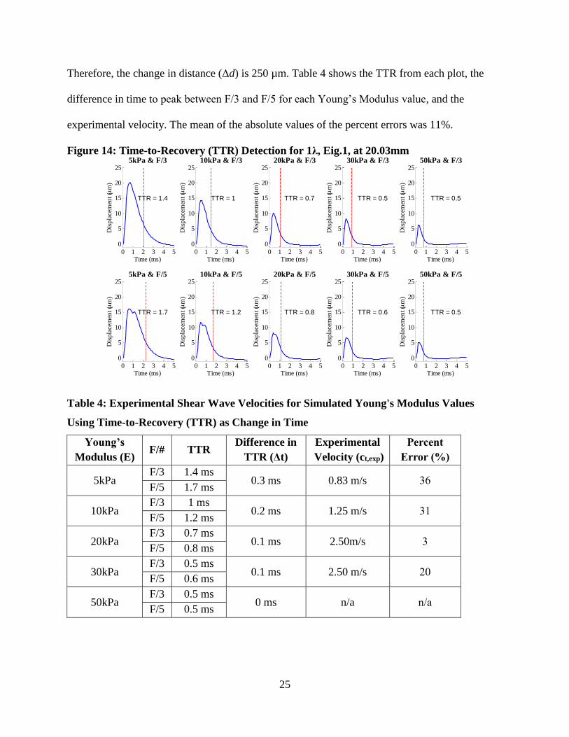
Time-to-recovery (TTR) is the timespan over which at which the waveform has
recovered 2/3 of the way from its peak. Figure 14 shows the TTR for 1λ kernel at 20.03 mm and
indicates the value of the TTP for each plot. It was hypothesized that the difference between the
TTP for F/3 and F/5 could be used to calculate the experimental velocity. The change in distance
(Δd) for this method is the difference between half the lateral span of the resolution cells for F/3
and F/5. This distance can be calculated in terms of wavelength (λ) and F/# similar:
Δ𝑑 =1
2(𝐹/5 − 𝐹/3) ∗ 𝜆.
0 1 2 3 4 5
0
5
10
15
20
TTP = 0.7
5kPa & F/3
Time (ms)
Dis
pla
cem
ent
(m
)
0 1 2 3 4 5-5
0
5
10
15
20
TTP = 0.6
5kPa & F/5
Time (ms)
Dis
pla
cem
ent
(m
)
0 1 2 3 4 5
0
5
10
15
20
TTP = 0.5
10kPa & F/3
Time (ms)
Dis
pla
cem
ent
(m
)
0 1 2 3 4 5-5
0
5
10
15
20
TTP = 0.5
10kPa & F/5
Time (ms)
Dis
pla
cem
ent
(m
)
0 1 2 3 4 5
0
5
10
15
20
TTP = 0.4
Mean of 10 Seeds with Time-to-Peak Detection for 1, Focused at 20.03mm, Eig.1
20kPa & F/3
Time (ms)
Dis
pla
cem
ent
(m
)
0 1 2 3 4 5-5
0
5
10
15
20
TTP = 0.4
20kPa & F/5
Time (ms)
Dis
pla
cem
ent
(m
)
0 1 2 3 4 5
0
5
10
15
20
TTP = 0.4
30kPa & F/3
Time (ms)
Dis
pla
cem
ent
(m
)
0 1 2 3 4 5-5
0
5
10
15
20
TTP = 0.4
30kPa & F/5
Time (ms)
Dis
pla
cem
ent
(m
)
0 1 2 3 4 5
0
5
10
15
20
TTP = 0.3
50kPa & F/3
Time (ms)
Dis
pla
cem
ent
(m
)
0 1 2 3 4 5-5
0
5
10
15
20
TTP = 0.3
50kPa & F/5
Time (ms)
Dis
pla
cem
ent
(m
)
25
Therefore, the change in distance (Δd) is 250 µm. Table 4 shows the TTR from each plot, the
difference in time to peak between F/3 and F/5 for each Young’s Modulus value, and the
experimental velocity. The mean of the absolute values of the percent errors was 11%.
Figure 14: Time-to-Recovery (TTR) Detection for 1λ, Eig.1, at 20.03mm
Table 4: Experimental Shear Wave Velocities for Simulated Young's Modulus Values
Using Time-to-Recovery (TTR) as Change in Time
Young’s
Modulus (E) F/# TTR
Difference in
TTR (Δt)
Experimental
Velocity (ct,exp)
Percent
Error (%)
5kPa F/3 1.4 ms
0.3 ms 0.83 m/s 36 F/5 1.7 ms
10kPa F/3 1 ms
0.2 ms 1.25 m/s 31 F/5 1.2 ms
20kPa F/3 0.7 ms
0.1 ms 2.50m/s 3 F/5 0.8 ms
30kPa F/3 0.5 ms
0.1 ms 2.50 m/s 20 F/5 0.6 ms
50kPa F/3 0.5 ms
0 ms n/a n/a F/5 0.5 ms
0 1 2 3 4 5
0
5
10
15
20
25
TTR = 1.4
5kPa & F/3
Time (ms)
Dis
pla
cem
ent
(m
)
0 1 2 3 4 5
0
5
10
15
20
25
TTR = 1.7
5kPa & F/5
Time (ms)
Dis
pla
cem
ent
(m
)
0 1 2 3 4 5
0
5
10
15
20
25
TTR = 1
10kPa & F/3
Time (ms)
Dis
pla
cem
ent
(m
)
0 1 2 3 4 5
0
5
10
15
20
25
TTR = 1.2
10kPa & F/5
Time (ms)
Dis
pla
cem
ent
(m
)
0 1 2 3 4 5
0
5
10
15
20
25
TTR = 0.7
Mean of 10 Seeds with Time-to-Recovery Detection for 1, Focused at 20.03mm, Eig.1
20kPa & F/3
Time (ms)D
isp
lace
men
t (
m)
0 1 2 3 4 5
0
5
10
15
20
25
TTR = 0.8
20kPa & F/5
Time (ms)
Dis
pla
cem
ent
(m
)0 1 2 3 4 5
0
5
10
15
20
25
TTR = 0.5
30kPa & F/3
Time (ms)
Dis
pla
cem
ent
(m
)
0 1 2 3 4 5
0
5
10
15
20
25
TTR = 0.6
30kPa & F/5
Time (ms)
Dis
pla
cem
ent
(m
)
0 1 2 3 4 5
0
5
10
15
20
25
TTR = 0.5
50kPa & F/3
Time (ms)
Dis
pla
cem
ent
(m
)
0 1 2 3 4 5
0
5
10
15
20
25
TTR = 0.5
50kPa & F/5
Time (ms)
Dis
pla
cem
ent
(m
)

26
Similar to the double peak results for experimental shear wave velocity, these
experimental shear wave velocities were an order of magnitude off from the expected shear wave
velocities. This is also likely due to the selection of change in distance as half the lateral span of
the resolution cell. The same ratio method was conducted for these experimental shear wave
velocities. Table 4 includes these values and the percent error of the experimental ratio compared
to the expected ratio. The ratios including 50kPa (rows indicated in grey) could not be calculated
due to the lack of experimental velocity. The other ratios (rows indicated in grey) ranged from
6% to 34% error. The mean of the absolute values of the percent errors was 21%.
Table 5: Expected and Experimental Shear Wave Velocities Ratios and Percent Error for
Time to Recovery (TTR)
Young’s
Modulus Ratio
Expected
Ratio
Experimental
Ratio
Percent
Error (%)
5kPa/10kPa 0.71 0.67 -6
5kPa/20kPa 0.50 0.33 -34
5kPa/30kPa 0.41 0.33 -20
5kPa/50kPa 0.32 n/a n/a
10kPa/20kPa 0.71 0.50 -30
10kPa/30kPa 0.58 0.50 -14
10kPa/50kPa 0.45 n/a n/a
20kPa/30kPa 0.82 1 22
20kPa/50kPa 0.63 n/a n/a
30kPa/50kPa 0.77 n/a n/a

27
CHAPTER 5: CONCLUSION & FUTURE DIRECTION
This project attempted to use PCA to reconstruct shear waves propagating away from the
region of excitation (ROE) of an acoustic radiation force impulse. It was hypothesized that by
using a narrowly focused push beam (F/0.75) and a wide track beam (F/3 or F/5), it would be
possible to detect the shear wave propagation. Furthermore, it was hypothesized that the first
eigenvalue extracted by PCA would encode information on the initial shear wave, and the second
eigenvalue would encode information on the shear wave later in time, once it had propagated
away from the ROE. At this time eigenvalues beyond the first do not seem to encode any
information regarding shear wave propagation.
Although the initial hypothesis did not hold, double peaks—not characteristic of shear
wave waveforms—were detected in certain kernels of the F/5 tracked eigenvector 1. Future work
will need to be conducted to investigate why certain kernels displayed this double peak more
prominently than others. The detection of double peaks led to a new hypothesis that PCA had
merged what was expected to be two separate signals into the same eigenvector. This would
make sense if the waveforms were not orthogonal. As stiffness increased, the distance between
the two peaks appeared to decrease. This would make sense if these peaks indicated two different
times at which the shear wave was detected because shear waves propagate faster in stiffer
materials.
At this time, it is still unclear where the second shear wave (i.e. the second peak) was
detected. Initially, it was hypothesized that it was extracted from the edge of the resolution cell.
This would mean that the time between the peaks would indicate the time it took the shear wave

28
to span half of the resolution cell. Calculation of experimental shear wave velocity based on this
hypothesis resulted in velocities an order of magnitude lower than the expected shear wave
velocity. The results were limited by the time resolution of the samples, 0.1ms. Although the
experimental shear wave velocities were not accurate, the ratios of the shear wave velocities for
different stiffnesses resulted in values within 11% of the expected shear wave velocities. If the
distance corresponding to the timespan between the peaks can be determined, this method may
be valid way of measuring shear velocity quantitatively.
Other methods of relatively measuring shear wave velocity were also attempted: time-to-
peak and time-to-recovery. Time-to-peak was not successful because the difference in time-to-
peak for F/3 and F/5 for most stiffness was equal to zero. The difference in time-to-recovery for
F/3 and F/5 were different, but the experimental shear wave velocities calculated in this method
were also an order of magnitude too small. When the ratios for time-to-recovery velocities were
compared to the expected velocities, there was significantly more error than the results from the
double peaks method. Before dismissing either time-to-peak or time-to-recovery, it would be
useful to examine other kernels as well as other focuses of the kernels (beyond 20mm).
Although more work needs to do be done in simulation, the hope is that this work will be
implemented in tissue mimicking phantoms. These phantoms may be constructed from materials
with the same Young’s modulus values used in simulation. This will allow the experimental
results to be compared to the simulated ones. Following testing in tissue mimicking materials,
this method will eventually be implemented in tissue.

29
APPENDIX 1: SUPPLEMENTARY MATLAB FIGURES FOR ENTIRE DATA SET
0 1 2 3 4 5-200
-100
0
100
200
Time (ms)
Dis
pla
cem
ent
(m
)
5kPa & F/3
Mean
0 1 2 3 4 5-200
-100
0
100
200
Time (ms)
Dis
pla
cem
ent
(m
)
5kPa & F/5
Mean
0 1 2 3 4 5-200
-100
0
100
200
Time (ms)
Dis
pla
cem
ent
(m
)
10kPa & F/3
Mean
0 1 2 3 4 5-200
-100
0
100
200
Time (ms)
Dis
pla
cem
ent
(m
)
10kPa & F/5
Mean
0 1 2 3 4 5-200
-100
0
100
200
Time (ms)
Dis
pla
cem
ent
(m
)
10 Seeds and Mean for No Kernel, Eig.3
20kPa & F/3
Mean
0 1 2 3 4 5-200
-100
0
100
200
Time (ms)
Dis
pla
cem
ent
(m
)
20kPa & F/5
Mean
0 1 2 3 4 5-200
-100
0
100
200
Time (ms)
Dis
pla
cem
ent
(m
)
30kPa & F/3
Mean
0 1 2 3 4 5-200
-100
0
100
200
Time (ms)D
isp
lace
men
t (
m)
30kPa & F/5
Mean
0 1 2 3 4 5-200
-100
0
100
200
Time (ms)
Dis
pla
cem
ent
(m
)
50kPa & F/3
Mean
0 1 2 3 4 5-200
-100
0
100
200
Time (ms)
Dis
pla
cem
ent
(m
)
50kPa & F/5
Mean
0 1 2 3 4 5-400
-200
0
200
400
Time (ms)
Dis
pla
cem
ent
(m
)
5kPa & F/3
Mean
0 1 2 3 4 5-400
-200
0
200
400
Time (ms)
Dis
pla
cem
ent
(m
)
5kPa & F/5
Mean
0 1 2 3 4 5-400
-200
0
200
400
Time (ms)
Dis
pla
cem
ent
(m
)
10kPa & F/3
Mean
0 1 2 3 4 5-400
-200
0
200
400
Time (ms)
Dis
pla
cem
ent
(m
)
10kPa & F/5
Mean
0 1 2 3 4 5-400
-200
0
200
400
Time (ms)
Dis
pla
cem
ent
(m
)
10 Seeds and Mean for No Kernel, Eig.4
20kPa & F/3
Mean
0 1 2 3 4 5-400
-200
0
200
400
Time (ms)
Dis
pla
cem
ent
(m
)
20kPa & F/5
Mean
0 1 2 3 4 5-400
-200
0
200
400
Time (ms)
Dis
pla
cem
ent
(m
)
30kPa & F/3
Mean
0 1 2 3 4 5-400
-200
0
200
400
Time (ms)
Dis
pla
cem
ent
(m
)
30kPa & F/5
Mean
0 1 2 3 4 5-400
-200
0
200
400
Time (ms)
Dis
pla
cem
ent
(m
)
50kPa & F/3
Mean
0 1 2 3 4 5-400
-200
0
200
400
Time (ms)
Dis
pla
cem
ent
(m
)
50kPa & F/5
Mean
30
0 1 2 3 4 5-400
-200
0
200
400
Time (ms)
Dis
pla
cem
ent
(m
)
5kPa & F/3
0 1 2 3 4 5-400
-200
0
200
400
Time (ms)
Dis
pla
cem
ent
(m
)
5kPa & F/5
Mean
0 1 2 3 4 5-400
-200
0
200
400
Time (ms)D
isp
lace
men
t (
m)
10kPa & F/3
Mean
0 1 2 3 4 5-400
-200
0
200
400
Time (ms)
Dis
pla
cem
ent
(m
)
10kPa & F/5
Mean
0 1 2 3 4 5-400
-200
0
200
400
Time (ms)
Dis
pla
cem
ent
(m
)
10 Seeds and Mean for No Kernel, Eig.5
20kPa & F/3
Mean
0 1 2 3 4 5-400
-200
0
200
400
Time (ms)
Dis
pla
cem
ent
(m
)
20kPa & F/5
0 1 2 3 4 5-400
-200
0
200
400
Time (ms)
Dis
pla
cem
ent
(m
)
30kPa & F/3
Mean
0 1 2 3 4 5-400
-200
0
200
400
Time (ms)
Dis
pla
cem
ent
(m
)
30kPa & F/5
0 1 2 3 4 5-400
-200
0
200
400
Time (ms)
Dis
pla
cem
ent
(m
)
50kPa & F/3
Mean
0 1 2 3 4 5-400
-200
0
200
400
Time (ms)
Dis
pla
cem
ent
(m
)
50kPa & F/5
Mean
1 2 3 4 5
0
2
4
6
Seed 0 & F/3
Time (ms)
Dis
pla
cem
ent
(m
)
1 2 3 4 5
0
1
2
3
4
Seed 1 & F/3
Time (ms)
Dis
pla
cem
ent
(m
)
1 2 3 4 5
0
1
2
3
4 Seeds and Mean for No Kernel, Eig.1
Seed 2 & F/3
Time (ms)
Dis
pla
cem
ent
(m
)
1 2 3 4 5
0
2
4
6
Seed 3 & F/3
Time (ms)
Dis
pla
cem
ent
(m
)
1 2 3 4 5
0
1
2
3
4
5
Mean Seeds & F/3
Time (ms)
Dis
pla
cem
ent
(m
)
1 2 3 4 5
0
1
2
3
4
5
Seed 0 & F/5
Time (ms)
Dis
pla
cem
ent
(m
)
1 2 3 4 5
0
1
2
3
Seed 1 & F/5
Time (ms)
Dis
pla
cem
ent
(m
)
1 2 3 4 5
0
1
2
3
Seed 2 & F/5
Time (ms)
Dis
pla
cem
ent
(m
)
1 2 3 4 5
0
1
2
3
4
5
Seed 3 & F/5
Time (ms)
Dis
pla
cem
ent
(m
)
1 2 3 4 5
0
1
2
3
4
Mean Seeds & F/5
Time (ms)
Dis
pla
cem
ent
(m
)
5kPa
10kPa
20kPa
30kPa
50kPa
5kPa
10kPa
20kPa
30kPa
50kPa
5kPa
10kPa
20kPa
30kPa
50kPa
5kPa
10kPa
20kPa
30kPa
50kPa

31
0 1 2 3 4 5
0
2
4
6
Seed 4 & F/3
Time (ms)
Dis
pla
cem
ent
(m
)
0 1 2 3 4 5
0
2
4
6
Seed 5 & F/3
Time (ms)
Dis
pla
cem
ent
(m
)
0 1 2 3 4 5
0
2
4
6
4 Seeds and Mean for No Kernel, Eig.1
Seed 6 & F/3
Time (ms)
Dis
pla
cem
ent
(m
)
0 1 2 3 4 5
0
2
4
6
Seed 7 & F/3
Time (ms)
Dis
pla
cem
ent
(m
)
0 1 2 3 4 5
0
2
4
6
Mean Seeds & F/3
Time (ms)
Dis
pla
cem
ent
(m
)
0 1 2 3 4 5
0
2
4
6Seed 4 & F/5
Time (ms)
Dis
pla
cem
ent
(m
)
0 1 2 3 4 5
0
2
4
6Seed 5 & F/5
Time (ms)
Dis
pla
cem
ent
(m
)
0 1 2 3 4 5
0
2
4
6Seed 6 & F/5
Time (ms)
Dis
pla
cem
ent
(m
)0 1 2 3 4 5
0
2
4
6Seed 7 & F/5
Time (ms)
Dis
pla
cem
ent
(m
)
0 1 2 3 4 5
0
2
4
6Mean Seeds & F/5
Time (ms)
Dis
pla
cem
ent
(m
)
5kPa
10kPa
20kPa
30kPa
50kPa
5kPa
10kPa
20kPa
30kPa
50kPa
5kPa
10kPa
20kPa
30kPa
50kPa
5kPa
10kPa
20kPa
30kPa
50kPa
0 1 2 3 4 5
0
2
4
6
Seed 8 & F/3
Time (ms)
Dis
pla
cem
ent
(m
)
0 1 2 3 4 5
0
2
4
6
2 Seeds and Mean for No Kernel, Eig.1
Seed 9 & F/3
Time (ms)
Dis
pla
cem
ent
(m
)
0 1 2 3 4 5
0
2
4
6
Mean Seeds & F/3
Time (ms)
Dis
pla
cem
ent
(m
)
0 1 2 3 4 5
0
2
4
6Seed 8 & F/5
Time (ms)
Dis
pla
cem
ent
(m
)
0 1 2 3 4 5
0
2
4
6Seed 9 & F/5
Time (ms)
Dis
pla
cem
ent
(m
)
0 1 2 3 4 5
0
2
4
6Mean Seeds & F/5
Time (ms)
Dis
pla
cem
ent
(m
)
5kPa
10kPa
20kPa
30kPa
50kPa
5kPa
10kPa
20kPa
30kPa
50kPa
5kPa
10kPa
20kPa
30kPa
50kPa
5kPa
10kPa
20kPa
30kPa
50kPa

32
APPENDIX 2: SUPPLEMENTARY MATLAB FIGURES FOR KERNELS
1λ Figures
0 1 2 3 4 5
0
10
20
30
Time (ms)
Dis
pla
cem
ent
(m
)
5kPa & F/3
Mean
0 1 2 3 4 5
0
10
20
30
40
Time (ms)
Dis
pla
cem
ent
(m
)
5kPa & F/5
Mean
0 1 2 3 4 5
0
10
20
30
Time (ms)
Dis
pla
cem
ent
(m
)
10kPa & F/3
Mean
0 1 2 3 4 5
0
10
20
30
40
Time (ms)
Dis
pla
cem
ent
(m
)
10kPa & F/5
Mean
0 1 2 3 4 5
0
10
20
30
Time (ms)
Dis
pla
cem
ent
(m
)
10 Seeds and Mean for 1 , Focused at 20 mm, Eig.1
20kPa & F/3
Mean
0 1 2 3 4 5
0
10
20
30
40
Time (ms)
Dis
pla
cem
ent
(m
)20kPa & F/5
Mean
0 1 2 3 4 5
0
10
20
30
Time (ms)
Dis
pla
cem
ent
(m
)
30kPa & F/3
Mean
0 1 2 3 4 5
0
10
20
30
40
Time (ms)
Dis
pla
cem
ent
(m
)
30kPa & F/5
Mean
0 1 2 3 4 5
0
10
20
30
Time (ms)
Dis
pla
cem
ent
(m
)
50kPa & F/3
Mean
0 1 2 3 4 5
0
10
20
30
40
Time (ms)
Dis
pla
cem
ent
(m
)
50kPa & F/5
Mean
1 2 3 4 50
5
10
15
20
25
5kPa & F/3
Time (ms)
Dis
pla
cem
ent
(m
)
1 2 3 4 50
10
20
305kPa & F/5
Time (ms)
Dis
pla
cem
ent
(m
)
1 2 3 4 50
5
10
15
20
25
10kPa & F/3
Time (ms)
Dis
pla
cem
ent
(m
)
1 2 3 4 50
10
20
3010kPa & F/5
Time (ms)
Dis
pla
cem
ent
(m
)
1 2 3 4 50
5
10
15
20
25
Mean with Standard Deviation of 10 Seeds 1, Focused at 20mm, Eig.1
20kPa & F/3
Time (ms)
Dis
pla
cem
ent
(m
)
1 2 3 4 50
10
20
3020kPa & F/5
Time (ms)
Dis
pla
cem
ent
(m
)
1 2 3 4 50
5
10
15
20
25
30kPa & F/3
Time (ms)
Dis
pla
cem
ent
(m
)
1 2 3 4 50
10
20
3030kPa & F/5
Time (ms)
Dis
pla
cem
ent
(m
)
1 2 3 4 50
5
10
15
20
25
50kPa & F/3
Time (ms)
Dis
pla
cem
ent
(m
)
1 2 3 4 50
10
20
3050kPa & F/5
Time (ms)
Dis
pla
cem
ent
(m
)

33
0 1 2 3 4 5
0
5
10
15
20
25Seed 0 & F/3
Time (ms)
Dis
pla
cem
ent
(m
)
0 1 2 3 4 5
0
5
10
15
20
25Seed 1 & F/3
Time (ms)
Dis
pla
cem
ent
(m
)
0 1 2 3 4 5
0
5
10
15
20
25
4 Seeds and Mean for 1, Focused at 20mm, Eig.1
Seed 2 & F/3
Time (ms)
Dis
pla
cem
ent
(m
)
0 1 2 3 4 5
0
5
10
15
20
25Seed 3 & F/3
Time (ms)
Dis
pla
cem
ent
(m
)
0 1 2 3 4 5
0
5
10
15
20
25Mean Seeds & F/3
Time (ms)
Dis
pla
cem
ent
(m
)
0 1 2 3 4 5
0
5
10
15
20Seed 0 & F/5
Time (ms)
Dis
pla
cem
ent
(m
)
0 1 2 3 4 5
0
5
10
15
20Seed 1 & F/5
Time (ms)
Dis
pla
cem
ent
(m
)
0 1 2 3 4 5
0
5
10
15
20Seed 2 & F/5
Time (ms)
Dis
pla
cem
ent
(m
)0 1 2 3 4 5
0
5
10
15
20Seed 3 & F/5
Time (ms)
Dis
pla
cem
ent
(m
)
0 1 2 3 4 5
0
5
10
15
20Mean Seeds & F/5
Time (ms)
Dis
pla
cem
ent
(m
)
5kPa
10kPa
20kPa
30kPa
50kPa
5kPa
10kPa
20kPa
30kPa
50kPa
5kPa
10kPa
20kPa
30kPa
50kPa
5kPa
10kPa
20kPa
30kPa
50kPa
0 1 2 3 4 50
10
20
30Seed 4 & F/3
Time (ms)
Dis
pla
cem
ent
(m
)
0 1 2 3 4 50
10
20
30Seed 5 & F/3
Time (ms)
Dis
pla
cem
ent
(m
)
0 1 2 3 4 50
10
20
30
4 Seeds and Mean for 1, Focused at 20mm, Eig.1
Seed 6 & F/3
Time (ms)
Dis
pla
cem
ent
(m
)
0 1 2 3 4 50
10
20
30Seed 7 & F/3
Time (ms)
Dis
pla
cem
ent
(m
)
0 1 2 3 4 50
10
20
30Mean Seeds & F/3
Time (ms)D
isp
lace
men
t (
m)
0 1 2 3 4 50
10
20
30
Seed 4 & F/5
Time (ms)
Dis
pla
cem
ent
(m
)
0 1 2 3 4 50
10
20
30
Seed 5 & F/5
Time (ms)
Dis
pla
cem
ent
(m
)
0 1 2 3 4 50
10
20
30
Seed 6 & F/5
Time (ms)
Dis
pla
cem
ent
(m
)
0 1 2 3 4 50
10
20
30
Seed 7 & F/5
Time (ms)
Dis
pla
cem
ent
(m
)
0 1 2 3 4 50
10
20
30
Mean Seeds & F/5
Time (ms)
Dis
pla
cem
ent
(m
)
5kPa
10kPa
20kPa
30kPa
50kPa
5kPa
10kPa
20kPa
30kPa
50kPa
5kPa
10kPa
20kPa
30kPa
50kPa
5kPa
10kPa
20kPa
30kPa
50kPa
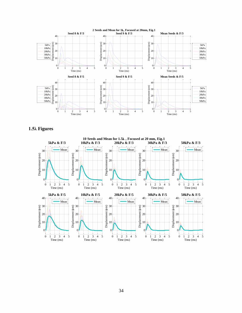
34
1.5λ Figures
0 1 2 3 4 50
10
20
30
40Seed 8 & F/3
Time (ms)
Dis
pla
cem
ent
(m
)
0 1 2 3 4 50
10
20
30
40
2 Seeds and Mean for 1, Focused at 20mm, Eig.1
Seed 9 & F/3
Time (ms)
Dis
pla
cem
ent
(m
)
0 1 2 3 4 50
10
20
30
40Mean Seeds & F/3
Time (ms)
Dis
pla
cem
ent
(m
)
0 1 2 3 4 50
10
20
30
40
Seed 8 & F/5
Time (ms)
Dis
pla
cem
ent
(m
)
0 1 2 3 4 50
10
20
30
40
Seed 9 & F/5
Time (ms)
Dis
pla
cem
ent
(m
)
0 1 2 3 4 50
10
20
30
40
Mean Seeds & F/5
Time (ms)
Dis
pla
cem
ent
(m
)
5kPa
10kPa
20kPa
30kPa
50kPa
5kPa
10kPa
20kPa
30kPa
50kPa
5kPa
10kPa
20kPa
30kPa
50kPa
5kPa
10kPa
20kPa
30kPa
50kPa
0 1 2 3 4 5
0
10
20
30
Time (ms)
Dis
pla
cem
ent
(m
)
5kPa & F/3
Mean
0 1 2 3 4 5
0
10
20
30
40
Time (ms)
Dis
pla
cem
ent
(m
)
5kPa & F/5
Mean
0 1 2 3 4 5
0
10
20
30
Time (ms)
Dis
pla
cem
ent
(m
)
10kPa & F/3
Mean
0 1 2 3 4 5
0
10
20
30
40
Time (ms)
Dis
pla
cem
ent
(m
)
10kPa & F/5
Mean
0 1 2 3 4 5
0
10
20
30
Time (ms)
Dis
pla
cem
ent
(m
)
10 Seeds and Mean for 1.5 , Focused at 20 mm, Eig.1
20kPa & F/3
Mean
0 1 2 3 4 5
0
10
20
30
40
Time (ms)
Dis
pla
cem
ent
(m
)
20kPa & F/5
Mean
0 1 2 3 4 5
0
10
20
30
Time (ms)
Dis
pla
cem
ent
(m
)
30kPa & F/3
Mean
0 1 2 3 4 5
0
10
20
30
40
Time (ms)
Dis
pla
cem
ent
(m
)
30kPa & F/5
Mean
0 1 2 3 4 5
0
10
20
30
Time (ms)
Dis
pla
cem
ent
(m
)
50kPa & F/3
Mean
0 1 2 3 4 5
0
10
20
30
40
Time (ms)
Dis
pla
cem
ent
(m
)
50kPa & F/5
Mean
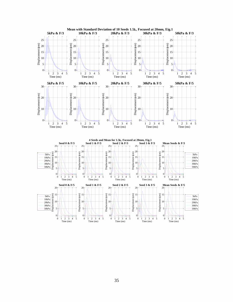
35
1 2 3 4 50
5
10
15
20
25
5kPa & F/3
Time (ms)
Dis
pla
cem
ent
(m
)
1 2 3 4 50
10
20
305kPa & F/5
Time (ms)
Dis
pla
cem
ent
(m
)
1 2 3 4 50
5
10
15
20
25
10kPa & F/3
Time (ms)
Dis
pla
cem
ent
(m
)
1 2 3 4 50
10
20
3010kPa & F/5
Time (ms)
Dis
pla
cem
ent
(m
)1 2 3 4 5
0
5
10
15
20
25
Mean with Standard Deviation of 10 Seeds 1.5, Focused at 20mm, Eig.1
20kPa & F/3
Time (ms)
Dis
pla
cem
ent
(m
)
1 2 3 4 50
10
20
3020kPa & F/5
Time (ms)
Dis
pla
cem
ent
(m
)
1 2 3 4 50
5
10
15
20
25
30kPa & F/3
Time (ms)
Dis
pla
cem
ent
(m
)
1 2 3 4 50
10
20
3030kPa & F/5
Time (ms)
Dis
pla
cem
ent
(m
)
1 2 3 4 50
5
10
15
20
25
50kPa & F/3
Time (ms)
Dis
pla
cem
ent
(m
)
1 2 3 4 50
10
20
3050kPa & F/5
Time (ms)
Dis
pla
cem
ent
(m
)
0 1 2 3 4 5
0
5
10
15
20
25Seed 0 & F/3
Time (ms)
Dis
pla
cem
ent
(m
)
0 1 2 3 4 5
0
5
10
15
20
25Seed 1 & F/3
Time (ms)
Dis
pla
cem
ent
(m
)
0 1 2 3 4 5
0
5
10
15
20
25
4 Seeds and Mean for 1.5, Focused at 20mm, Eig.1
Seed 2 & F/3
Time (ms)
Dis
pla
cem
ent
(m
)
0 1 2 3 4 5
0
5
10
15
20
25Seed 3 & F/3
Time (ms)
Dis
pla
cem
ent
(m
)
0 1 2 3 4 5
0
5
10
15
20
25Mean Seeds & F/3
Time (ms)
Dis
pla
cem
ent
(m
)
0 1 2 3 4 5
0
5
10
15
20Seed 0 & F/5
Time (ms)
Dis
pla
cem
ent
(m
)
0 1 2 3 4 5
0
5
10
15
20Seed 1 & F/5
Time (ms)
Dis
pla
cem
ent
(m
)
0 1 2 3 4 5
0
5
10
15
20Seed 2 & F/5
Time (ms)
Dis
pla
cem
ent
(m
)
0 1 2 3 4 5
0
5
10
15
20Seed 3 & F/5
Time (ms)
Dis
pla
cem
ent
(m
)
0 1 2 3 4 5
0
5
10
15
20Mean Seeds & F/5
Time (ms)
Dis
pla
cem
ent
(m
)
5kPa
10kPa
20kPa
30kPa
50kPa
5kPa
10kPa
20kPa
30kPa
50kPa
5kPa
10kPa
20kPa
30kPa
50kPa
5kPa
10kPa
20kPa
30kPa
50kPa
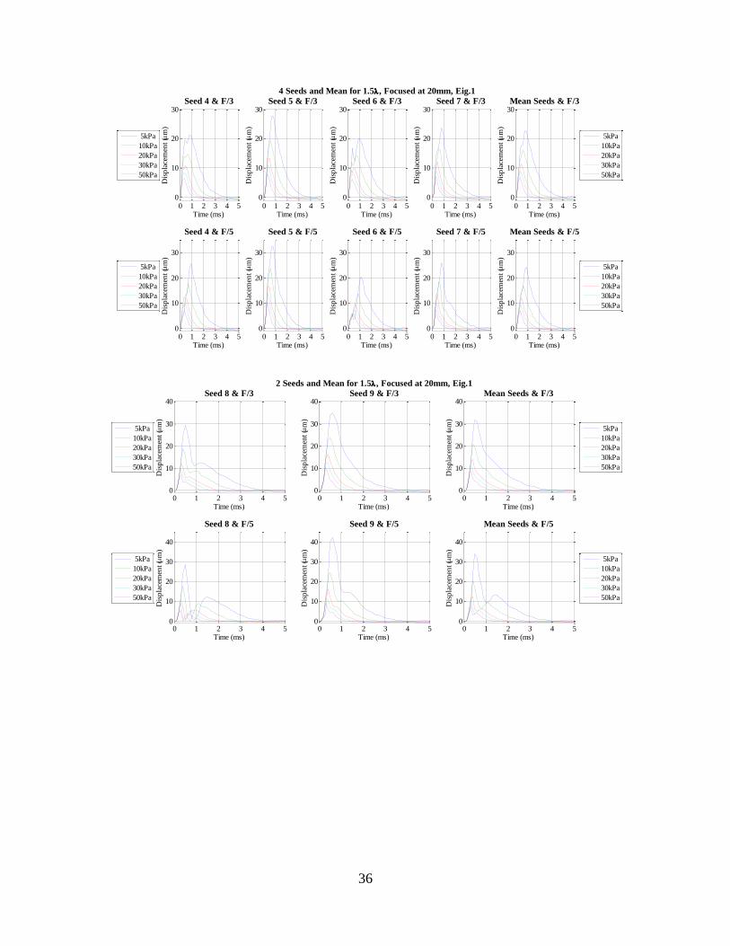
36
0 1 2 3 4 50
10
20
30Seed 4 & F/3
Time (ms)
Dis
pla
cem
ent
(m
)
0 1 2 3 4 50
10
20
30Seed 5 & F/3
Time (ms)
Dis
pla
cem
ent
(m
)
0 1 2 3 4 50
10
20
30
4 Seeds and Mean for 1.5, Focused at 20mm, Eig.1
Seed 6 & F/3
Time (ms)
Dis
pla
cem
ent
(m
)
0 1 2 3 4 50
10
20
30Seed 7 & F/3
Time (ms)
Dis
pla
cem
ent
(m
)
0 1 2 3 4 50
10
20
30Mean Seeds & F/3
Time (ms)
Dis
pla
cem
ent
(m
)
0 1 2 3 4 50
10
20
30
Seed 4 & F/5
Time (ms)
Dis
pla
cem
ent
(m
)
0 1 2 3 4 50
10
20
30
Seed 5 & F/5
Time (ms)
Dis
pla
cem
ent
(m
)
0 1 2 3 4 50
10
20
30
Seed 6 & F/5
Time (ms)
Dis
pla
cem
ent
(m
)0 1 2 3 4 5
0
10
20
30
Seed 7 & F/5
Time (ms)
Dis
pla
cem
ent
(m
)
0 1 2 3 4 50
10
20
30
Mean Seeds & F/5
Time (ms)
Dis
pla
cem
ent
(m
)
5kPa
10kPa
20kPa
30kPa
50kPa
5kPa
10kPa
20kPa
30kPa
50kPa
5kPa
10kPa
20kPa
30kPa
50kPa
5kPa
10kPa
20kPa
30kPa
50kPa
0 1 2 3 4 50
10
20
30
40Seed 8 & F/3
Time (ms)
Dis
pla
cem
ent
(m
)
0 1 2 3 4 50
10
20
30
40
2 Seeds and Mean for 1.5, Focused at 20mm, Eig.1
Seed 9 & F/3
Time (ms)
Dis
pla
cem
ent
(m
)
0 1 2 3 4 50
10
20
30
40Mean Seeds & F/3
Time (ms)
Dis
pla
cem
ent
(m
)
0 1 2 3 4 50
10
20
30
40
Seed 8 & F/5
Time (ms)
Dis
pla
cem
ent
(m
)
0 1 2 3 4 50
10
20
30
40
Seed 9 & F/5
Time (ms)
Dis
pla
cem
ent
(m
)
0 1 2 3 4 50
10
20
30
40
Mean Seeds & F/5
Time (ms)
Dis
pla
cem
ent
(m
)
5kPa
10kPa
20kPa
30kPa
50kPa
5kPa
10kPa
20kPa
30kPa
50kPa
5kPa
10kPa
20kPa
30kPa
50kPa
5kPa
10kPa
20kPa
30kPa
50kPa

37
3λ Figures
0 1 2 3 4 5
0
10
20
30
Time (ms)
Dis
pla
cem
ent
(m
)5kPa & F/3
Mean
0 1 2 3 4 5
0
10
20
30
40
Time (ms)
Dis
pla
cem
ent
(m
)
5kPa & F/5
Mean
0 1 2 3 4 5
0
10
20
30
Time (ms)
Dis
pla
cem
ent
(m
)
10kPa & F/3
Mean
0 1 2 3 4 5
0
10
20
30
40
Time (ms)
Dis
pla
cem
ent
(m
)
10kPa & F/5
Mean
0 1 2 3 4 5
0
10
20
30
Time (ms)
Dis
pla
cem
ent
(m
)
10 Seeds and Mean for 3 , Focused at 20 mm, Eig.1
20kPa & F/3
Mean
0 1 2 3 4 5
0
10
20
30
40
Time (ms)
Dis
pla
cem
ent
(m
)
20kPa & F/5
Mean
0 1 2 3 4 5
0
10
20
30
Time (ms)
Dis
pla
cem
ent
(m
)
30kPa & F/3
Mean
0 1 2 3 4 5
0
10
20
30
40
Time (ms)D
isp
lace
men
t (
m)
30kPa & F/5
Mean
0 1 2 3 4 5
0
10
20
30
Time (ms)
Dis
pla
cem
ent
(m
)
50kPa & F/3
Mean
0 1 2 3 4 5
0
10
20
30
40
Time (ms)
Dis
pla
cem
ent
(m
)
50kPa & F/5
Mean
1 2 3 4 50
5
10
15
20
25
5kPa & F/3
Time (ms)
Dis
pla
cem
ent
(m
)
1 2 3 4 50
10
20
305kPa & F/5
Time (ms)
Dis
pla
cem
ent
(m
)
1 2 3 4 50
5
10
15
20
25
10kPa & F/3
Time (ms)
Dis
pla
cem
ent
(m
)
1 2 3 4 50
10
20
3010kPa & F/5
Time (ms)
Dis
pla
cem
ent
(m
)
1 2 3 4 50
5
10
15
20
25
Mean with Standard Deviation of 10 Seeds 3, Focused at 20mm, Eig.1
20kPa & F/3
Time (ms)
Dis
pla
cem
ent
(m
)
1 2 3 4 50
10
20
3020kPa & F/5
Time (ms)
Dis
pla
cem
ent
(m
)
1 2 3 4 50
5
10
15
20
25
30kPa & F/3
Time (ms)
Dis
pla
cem
ent
(m
)
1 2 3 4 50
10
20
3030kPa & F/5
Time (ms)
Dis
pla
cem
ent
(m
)
1 2 3 4 50
5
10
15
20
25
50kPa & F/3
Time (ms)
Dis
pla
cem
ent
(m
)
1 2 3 4 50
10
20
3050kPa & F/5
Time (ms)
Dis
pla
cem
ent
(m
)

38
0 1 2 3 4 5
0
5
10
15
20
25Seed 0 & F/3
Time (ms)
Dis
pla
cem
ent
(m
)
0 1 2 3 4 5
0
5
10
15
20
25Seed 1 & F/3
Time (ms)
Dis
pla
cem
ent
(m
)
0 1 2 3 4 5
0
5
10
15
20
25
4 Seeds and Mean for 3, Focused at 20mm, Eig.1
Seed 2 & F/3
Time (ms)
Dis
pla
cem
ent
(m
)
0 1 2 3 4 5
0
5
10
15
20
25Seed 3 & F/3
Time (ms)
Dis
pla
cem
ent
(m
)
0 1 2 3 4 5
0
5
10
15
20
25Mean Seeds & F/3
Time (ms)
Dis
pla
cem
ent
(m
)
0 1 2 3 4 5
0
5
10
15
20
25Seed 0 & F/5
Time (ms)
Dis
pla
cem
ent
(m
)
0 1 2 3 4 5
0
5
10
15
20
25Seed 1 & F/5
Time (ms)
Dis
pla
cem
ent
(m
)
0 1 2 3 4 5
0
5
10
15
20
25Seed 2 & F/5
Time (ms)
Dis
pla
cem
ent
(m
)0 1 2 3 4 5
0
5
10
15
20
25Seed 3 & F/5
Time (ms)
Dis
pla
cem
ent
(m
)
0 1 2 3 4 5
0
5
10
15
20
25Mean Seeds & F/5
Time (ms)
Dis
pla
cem
ent
(m
)
5kPa
10kPa
20kPa
30kPa
50kPa
5kPa
10kPa
20kPa
30kPa
50kPa
5kPa
10kPa
20kPa
30kPa
50kPa
5kPa
10kPa
20kPa
30kPa
50kPa
0 1 2 3 4 50
10
20
30Seed 4 & F/3
Time (ms)
Dis
pla
cem
ent
(m
)
0 1 2 3 4 50
10
20
30Seed 5 & F/3
Time (ms)
Dis
pla
cem
ent
(m
)
0 1 2 3 4 50
10
20
30
4 Seeds and Mean for 3, Focused at 20mm, Eig.1
Seed 6 & F/3
Time (ms)
Dis
pla
cem
ent
(m
)
0 1 2 3 4 50
10
20
30Seed 7 & F/3
Time (ms)
Dis
pla
cem
ent
(m
)
0 1 2 3 4 50
10
20
30Mean Seeds & F/3
Time (ms)D
isp
lace
men
t (
m)
0 1 2 3 4 50
10
20
30
Seed 4 & F/5
Time (ms)
Dis
pla
cem
ent
(m
)
0 1 2 3 4 50
10
20
30
Seed 5 & F/5
Time (ms)
Dis
pla
cem
ent
(m
)
0 1 2 3 4 50
10
20
30
Seed 6 & F/5
Time (ms)
Dis
pla
cem
ent
(m
)
0 1 2 3 4 50
10
20
30
Seed 7 & F/5
Time (ms)
Dis
pla
cem
ent
(m
)
0 1 2 3 4 50
10
20
30
Mean Seeds & F/5
Time (ms)
Dis
pla
cem
ent
(m
)
5kPa
10kPa
20kPa
30kPa
50kPa
5kPa
10kPa
20kPa
30kPa
50kPa
5kPa
10kPa
20kPa
30kPa
50kPa
5kPa
10kPa
20kPa
30kPa
50kPa

39
Time-to-Peak (TTP)
0 1 2 3 4 50
10
20
30
40Seed 8 & F/3
Time (ms)
Dis
pla
cem
ent
(m
)
0 1 2 3 4 50
10
20
30
40
2 Seeds and Mean for 3, Focused at 20mm, Eig.1
Seed 9 & F/3
Time (ms)
Dis
pla
cem
ent
(m
)
0 1 2 3 4 50
10
20
30
40Mean Seeds & F/3
Time (ms)
Dis
pla
cem
ent
(m
)
0 1 2 3 4 50
10
20
30
40
Seed 8 & F/5
Time (ms)
Dis
pla
cem
ent
(m
)
0 1 2 3 4 50
10
20
30
40
Seed 9 & F/5
Time (ms)
Dis
pla
cem
ent
(m
)
0 1 2 3 4 50
10
20
30
40
Mean Seeds & F/5
Time (ms)
Dis
pla
cem
ent
(m
)
5kPa
10kPa
20kPa
30kPa
50kPa
5kPa
10kPa
20kPa
30kPa
50kPa
5kPa
10kPa
20kPa
30kPa
50kPa
5kPa
10kPa
20kPa
30kPa
50kPa
0 1 2 3 4 5
0
5
10
15
20
25
TTP = 0.8
5kPa & F/3
Time (ms)
Dis
pla
cem
ent
(m
)
0 1 2 3 4 5
0
5
10
15
20
25
TTP = 0.8
5kPa & F/5
Time (ms)
Dis
pla
cem
ent
(m
)
0 1 2 3 4 5
0
5
10
15
20
25
TTP = 0.6
10kPa & F/3
Time (ms)
Dis
pla
cem
ent
(m
)
0 1 2 3 4 5
0
5
10
15
20
25
TTP = 0.6
10kPa & F/5
Time (ms)
Dis
pla
cem
ent
(m
)
0 1 2 3 4 5
0
5
10
15
20
25
TTP = 0.4
Mean of 10 Seeds with Time-to-Peak Detection for 1.5, Focused at 20.03mm, Eig.1
20kPa & F/3
Time (ms)
Dis
pla
cem
ent
(m
)
0 1 2 3 4 5
0
5
10
15
20
25
TTP = 0.5
20kPa & F/5
Time (ms)
Dis
pla
cem
ent
(m
)
0 1 2 3 4 5
0
5
10
15
20
25
TTP = 0.4
30kPa & F/3
Time (ms)
Dis
pla
cem
ent
(m
)
0 1 2 3 4 5
0
5
10
15
20
25
TTP = 0.4
30kPa & F/5
Time (ms)
Dis
pla
cem
ent
(m
)
0 1 2 3 4 5
0
5
10
15
20
25
TTP = 0.3
50kPa & F/3
Time (ms)
Dis
pla
cem
ent
(m
)
0 1 2 3 4 5
0
5
10
15
20
25
TTP = 0.4
50kPa & F/5
Time (ms)
Dis
pla
cem
ent
(m
)

40
Time-to-Recovery (TTR)
0 1 2 3 4 5
0
5
10
15
20
25
TTP = 0.8
5kPa & F/3
Time (ms)
Dis
pla
cem
ent
(m
)
0 1 2 3 4 5
0
5
10
15
20
25
TTP = 0.8
5kPa & F/5
Time (ms)
Dis
pla
cem
ent
(m
)
0 1 2 3 4 5
0
5
10
15
20
25
TTP = 0.6
10kPa & F/3
Time (ms)
Dis
pla
cem
ent
(m
)
0 1 2 3 4 5
0
5
10
15
20
25
TTP = 0.6
10kPa & F/5
Time (ms)
Dis
pla
cem
ent
(m
)
0 1 2 3 4 5
0
5
10
15
20
25
TTP = 0.5
Mean of 10 Seeds with Time-to-Peak Detection for 3, Focused at 20.03mm, Eig.1
20kPa & F/3
Time (ms)
Dis
pla
cem
ent
(m
)
0 1 2 3 4 5
0
5
10
15
20
25
TTP = 0.5
20kPa & F/5
Time (ms)
Dis
pla
cem
ent
(m
)
0 1 2 3 4 5
0
5
10
15
20
25
TTP = 0.4
30kPa & F/3
Time (ms)
Dis
pla
cem
ent
(m
)
0 1 2 3 4 5
0
5
10
15
20
25
TTP = 0.4
30kPa & F/5
Time (ms)
Dis
pla
cem
ent
(m
)
0 1 2 3 4 5
0
5
10
15
20
25
TTP = 0.3
50kPa & F/3
Time (ms)
Dis
pla
cem
ent
(m
)
0 1 2 3 4 5
0
5
10
15
20
25
TTP = 0.4
50kPa & F/5
Time (ms)
Dis
pla
cem
ent
(m
)
0 1 2 3 4 5
0
5
10
15
20
25
TTR = 1.2
5kPa & F/3
Time (ms)
Dis
pla
cem
ent
(m
)
0 1 2 3 4 5
0
5
10
15
20
25
TTR = 1.4
5kPa & F/5
Time (ms)
Dis
pla
cem
ent
(m
)
0 1 2 3 4 5
0
5
10
15
20
25
TTR = 0.9
10kPa & F/3
Time (ms)
Dis
pla
cem
ent
(m
)
0 1 2 3 4 5
0
5
10
15
20
25
TTR = 1
10kPa & F/5
Time (ms)
Dis
pla
cem
ent
(m
)
0 1 2 3 4 5
0
5
10
15
20
25
TTR = 0.7
Mean of 10 Seeds with Time-to-Recovery Detection for 1.5, Focused at 20.03mm, Eig.1
20kPa & F/3
Time (ms)
Dis
pla
cem
ent
(m
)
0 1 2 3 4 5
0
5
10
15
20
25
TTR = 0.7
20kPa & F/5
Time (ms)
Dis
pla
cem
ent
(m
)
0 1 2 3 4 5
0
5
10
15
20
25
TTR = 0.5
30kPa & F/3
Time (ms)
Dis
pla
cem
ent
(m
)
0 1 2 3 4 5
0
5
10
15
20
25
TTR = 0.6
30kPa & F/5
Time (ms)
Dis
pla
cem
ent
(m
)
0 1 2 3 4 5
0
5
10
15
20
25
TTR = 0.5
50kPa & F/3
Time (ms)
Dis
pla
cem
ent
(m
)
0 1 2 3 4 5
0
5
10
15
20
25
TTR = 0.4
50kPa & F/5
Time (ms)
Dis
pla
cem
ent
(m
)

41
0 1 2 3 4 5
0
5
10
15
20
25
TTR = 1.2
5kPa & F/3
Time (ms)
Dis
pla
cem
ent
(m
)
0 1 2 3 4 5
0
5
10
15
20
25
TTR = 1.3
5kPa & F/5
Time (ms)
Dis
pla
cem
ent
(m
)
0 1 2 3 4 5
0
5
10
15
20
25
TTR = 0.9
10kPa & F/3
Time (ms)
Dis
pla
cem
ent
(m
)
0 1 2 3 4 5
0
5
10
15
20
25
TTR = 1
10kPa & F/5
Time (ms)
Dis
pla
cem
ent
(m
)
0 1 2 3 4 5
0
5
10
15
20
25
Mean of 10 Seeds with Time-to-Recovery Detection for 3, Focused at 20.03mm, Eig.1
20kPa & F/3
Time (ms)
Dis
pla
cem
ent
(m
)
TTR = 0.6
0 1 2 3 4 5
0
5
10
15
20
25
TTR = 0.7
20kPa & F/5
Time (ms)
Dis
pla
cem
ent
(m
)
0 1 2 3 4 5
0
5
10
15
20
25
TTR = 0.5
30kPa & F/3
Time (ms)
Dis
pla
cem
ent
(m
)
0 1 2 3 4 5
0
5
10
15
20
2530kPa & F/5
Time (ms)
Dis
pla
cem
ent
(m
)
TTR = 0.6
0 1 2 3 4 5
0
5
10
15
20
25
TTR = 0.5
50kPa & F/3
Time (ms)
Dis
pla
cem
ent
(m
)
0 1 2 3 4 5
0
5
10
15
20
25
TTR = 0.4
50kPa & F/5
Time (ms)
Dis
pla
cem
ent
(m
)
42
REFERENCES
Doherty, J., Trahey, G., Nightingale, K., & Palmeri, M. (2013). Acoustic radiation force
elasticity imaging in diagnostic ultrasound. IEEE Transactions on Ultrasonics,
Ferroelectrics, and Frequency Control, 60(4), 685–701.
http://doi.org/10.1109/TUFFC.2013.2617
Fahey, B. J., Nightingale, K. R., Nelson, R. C., Palmeri, M. L., & Trahey, G. E. (2005). Acoustic
radiation force impulse imaging of the abdomen: demonstration of feasibility and utility.
Ultrasound in Medicine & Biology, 31(9), 1185–98.
http://doi.org/10.1016/j.ultrasmedbio.2005.05.004
Gallippi, C. M., Nightingale, K. R., & Trahey, G. E. (2003). BSS-based filtering of physiological
and ARFI-induced tissue and blood motion. Ultrasound in Medicine & Biology, 29(11),
1583–1592. http://doi.org/10.1016/j.ultrasmedbio.2003.07.002
Gallippi, C. M., & Trahey, G. E. (2003). Blind Source Separation-Based Velocity Estimation
(BSSVE): Simulation and Clinical Results. In IEEE Ultrasonics Symposium (pp. 855–860).
Mauldin, F. W., Viola, F., & Walker, W. F. (2010). Complex principal components for robust
motion estimation. IEEE Transactions on Ultrasonics, Ferroelectrics, and Frequency
Control, 57(11), 2437–2449. http://doi.org/10.1109/TUFFC.2010.1710
Mazza, E., Nava, A., Hahnloser, D., Jochum, W., & Bajka, M. (2007). The mechanical response
of human liver and its relation to histology: an in vivo study. Medical Image Analysis,
11(6), 663–72. http://doi.org/10.1016/j.media.2007.06.010

43
Nightingale, K. (2012). Acoustic Radiation Force Impulse (ARFI) Imaging: a Review. Curr
Medical Imaging, 7(4), 328–339. http://doi.org/10.2174/157340511798038657.Acoustic
Olympus Corporation. (n.d.). Ultrasonic Flaw Detection Tutorial. Retrieved January 1, 2015,
from http://www.olympus-ims.com/en/ndt-tutorials/flaw-detection/
Palmeri, M. L., McAleavey, S. a., Trahey, G. E., & Nightingale, K. R. (2006). Ultrasonic
tracking of acoustic radiation force-induced displacements in homogeneous media. IEEE
Transactions on Ultrasonics, Ferroelectrics, and Frequency Control, 53(7), 1300–1313.
http://doi.org/10.1109/TUFFC.2006.1665078
Palmeri, M. L., Wang, M. H., Dahl, J. J., Frinkley, K. D., & Nightengale, K. R. (2009).
Quantifying Hepatic Shear Modulus In Vivo Using Acoustic Radiation Force, 34(4), 546–
558.
Szabo, T. L. (2014). Diagnostic Ultrasound Imaging: Inside Out. Diagnostic Ultrasound
Imaging: Inside Out. Elsevier. http://doi.org/10.1016/B978-0-12-396487-8.00003-3