Finite Element Methods for the PoissonEquation and its Applications

Charles Crook

July 30, 2013

Abstract

The finite element method is a fast computational method thatalso has a solid mathematical theory behind it. We visualize the fi-nite element approximation to the solution of the Poisson equationon different type of domains and observe the corresponding order ofconvergence. As a real-world application of the Poisson equation, weuse the finite element approximation to distinguish different cartooncharacters. Furthermore, we use the weighted Poisson equation arisingfrom the axisymmetric Poisson equation to distinguish axisymmetricthree-dimensional objects as well.

1 Poisson Equation with Homogenous Dirich-

let Boundary Conditions

Given the problem, find the function u that satisfies the following,

−∆u = F in Ωu = 0 on ∂Ω

where F is given data. The goal is to find a ‘good’ approximation to theexact solution u.

1

2 The Finite Element Method

The Finite Element Method is called so, since it starts by taking the inputteddomain and performing calculation to make the domain into now finitely manelements. The elements in my case are triangles.

With each mesh generated, that mesh has exactly one finite element ap-proximation uh. As the meshes become more refined, the uh changes tobetter approximate the exact solution. The main idea of the finite elementmethod is that it changes the infinite dimension problem into a finite dimen-sion problem. With the problem now converted into a finite dimension, itcan now be changed to a matrix system, using basis functions, for findingthe solution.

3 Finite Elements Subspace P 01

We now define the space we are working in to be P 01 , which means after the

domain has had the finite element method applied to it, each element insidehas a plane above it represented by the function ax+by+c, and the collectionof all functions over the domain has to be continuous and have zero boundaryconditions as well. The dimension of this space, P 0

1 , is the total number of

2

interior nodes.

4 Basis of P 01

Now, we construct a Φi for each interior node vi using the formula below,

Φi(vj) =

1, if i = j

0, if i 6= j

For example, to construct Φ1, you would have to plug in each interior nodeand find the value at each. At V1, Φ1 = 1, and at V2, V3, ..., V9, Φ1 = 0. Also,with the given initial condition, Φ1 = 0 on the boundary. Now connectingeach of the nodes together requires the use of the plane function, ax+ by+ c,from earlier.

5 Infinite Dimensional Problem ⇒ Finite Di-

mensional Problem

The infinite dimension problem, shown belowFind u ∈ H1

0 (Ω) s.t.∫Ω 5u5 v =

∫Ω Fv ∀v ∈ H1

0 (Ω)

where H10 = f :

∫Ωf 2 <∞,

∫Ω

[5f ]2 <∞, f = 0 on ∂Ω is now converted

to the finite dimensional problem, through the use of the Finite Element

3

Subspace, is shown below,

Find uh ∈ P 01 s.t.∫

Ω 5uh5 vh =∫

Ω Fvh ∀vh ∈ P 01

6 Finite Dimensional Problem ⇒ A~x = ~b

We convert the new finite problem down to a matrix system by using uh =n∑

i=1

ciΦi. ∫Ω 5uh5 vh =

∫Ω Fvh ∀vh ∈ P 0

1∫Ω 5(

n∑i=1

ciΦi)5 Φj =∫

Ω FΦj ∀j = 1, 2, . . . n

n∑i=1

ci∫

Ω 5Φi5 Φj =∫

Ω FΦj ∀j = 1, 2, . . . n

n∑i=1

ci∫

Ω5Φi5 Φj =

∫ΩFΦj ∀j = 1, 2, . . . n

A ~c = ~b

Where, the underlined red portion corresponds to the ith entry of ~c.The underlined blue portion indicates the ijth entry of the matrix A.The underlined green portion is jth entry of ~b.To find more a exact solution, requires a finer mesh. With this, the matrix

A will become larger with each mesh. So to find a more exact solution, youwill have wait longer for the program to finish.

4

7 Numerical Example

7.1 Example One

The problem for example one was,Find a function, u, with the given function, F, such that−∆u = F in Ωu = 0 on ∂Ω

I picked a ‘nice’ F such that u = xy(x− 1)(y − 1). By ‘nice’, I mean wherethe u = 0 on ∂Ω and u is a polynomial.

mesh ‖ u− uh ‖ OoC ‖ 5u−5uh ‖ OoC1 0.0186579226 —— 0.1074034163 ——2 0.0057148929 1.7070 0.0588911882 0.86693 0.0015087244 1.9214 0.0301758912 0.96474 0.0003824646 1.9799 0.0151826243 0.99105 0.0000959512 1.9950 0.0076032633 0.99776 0.0000240088 1.9987 0.0038031293 0.9994

The L2 error in the chart is reducing by about 1/4 each mesh. The order ofconvergence is the ratio of two meshes with respect to the largest edge length.Since the mesh size is decreasing by 1/2 each time, the order of convergenceconverges to 2.

5

Figure 1: Top View of the six meshes

Figure 2: Tilted View of the six meshes

6

7.2 Example Two

In Example 2, I decided to change the domain to be more complicated, byremoving part of the domain.

u = xy(x− 1)(y − 1)(x− 0.25)(y − 0.25)(y − 0.75)

mesh ‖ u− uh ‖ OoC ‖ 5u−5uh ‖ OoC2 0.0003341186 —— 0.0042327447 ——3 0.0001088289 1.6183 0.0024042537 0.81604 0.0000293177 1.8922 0.0012455389 0.94885 0.0000074747 1.9717 0.0006285406 0.98676 0.0000018781 1.9927 0.0003150047 0.9966

Figure 3: Top View of the five meshes

7

Figure 4: Tilted View of the five meshes

8

7.3 Example Three

For Example 3, I changed the domain to be more complicated by adding ahole inside it.

u = xy(x− 1)(y − 1)(x− 0.25)(y − 0.25)(y − 0.75)(x− 0.5)(x− 0.75)

mesh ‖ u− uh ‖ OoC ‖ 5u−5uh ‖ OoC3 0.0000069270 —— 0.0001657242 ——4 0.0000021446 1.6915 0.0000916471 0.85465 0.0000005696 1.9127 0.0000471180 0.95986 0.0000001447 1.9769 0.0000237300 0.9896

Figure 5: Top View of the four meshes

9

Figure 6: Tilted View of the four meshes

7.4 Conclusion

For examples 1 through 3, even though the domain got more complicated,the order of convergence still converged to 2. The reason why this happens isthat for each of the domains, I picked a ‘nice’ F such that u is a polynomialand all initial conditions hold true.

10

8 Order of Convergence relative to the Do-

main

In this section, we will show that as the domain gets more complex, whenF = 1, the Order of Convergence would not approach 2, but a number lessinstead.

−4 u = 1 in Ωu = 0 on ∂Ω

Meshes OoC Meshes OoC Meshes OoC Meshes OoC1,2,3 1.700569 1,2,3 1.725416 1,2,3 1.701380 2,3,4 1.6505892,3,4 1.745914 2,3,4 1.663195 2,3,4 1.644536 3,4,5 1.569222

Order of Convergence = log2

||uh1 − uh2||||uh2 − uh3||

Please note that the above formula is relative to meshes 1,2,3. The formula can be modified accordingly

to fit the desired meshes.

Notice that as the domain becomes more complicated, the exact solutionalso becomes more complicated, and this is why the Order of Convergencegoes down.

11

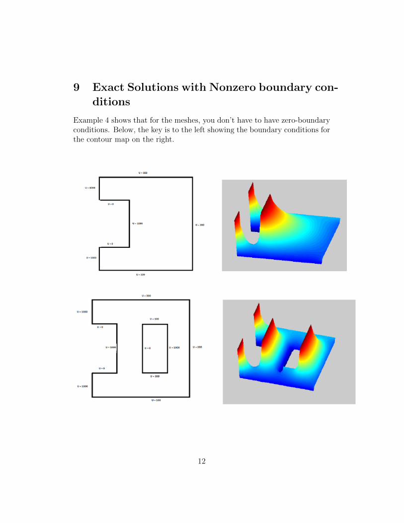
9 Exact Solutions with Nonzero boundary con-

ditions

Example 4 shows that for the meshes, you don’t have to have zero-boundaryconditions. Below, the key is to the left showing the boundary conditions forthe contour map on the right.

12

10 Shape Recognition using the Finite Ele-

ment Approximation of the Poisson Equa-

tion

In this section, I started to apply techniques learned in the paper “ShapeRepresentation and Classification Using the Poisson Equation.” [Gorelick, etal: 2006]

Mainly, I focused on using their formula for Φ, Φ = U + U2x + U2

y , andapplying to my domains, and then learning the special properties it upholds.For this section, I decided to use the block letters of the alphabet, H, J, L,T, and U.

Φ can be used to locate the corner of the domain where uh is changingmost rapidly or slowly, or where Φ is at its maximum or minimum. And if Iwanted to extract certain parts of the domain from their respective heights,the log(Φ) is calculated and graphed. From now onwards, any extractedpiece of the domain is taken from the log(Φ).

Figure 7: Contour Maps of the uhs

13

Figure 8: Contour Maps of U2x + U2

y

Figure 9: Contour Maps of Φ

14

Figure 10: Contour Maps of log(Φ)

15

11 Weighted Case of the Poisson Equation

I learned and applied the weighted case of the Poisson Equation to each ofthe block letters from the previous section. The weighted case is found bymultiplying x to each side of the formula, and now it becomes

N∑i=1

ci

∫Ω

5Φi5 Φjx =∫

ΩFΦjx

This weighted Poisson equation arises when performing dimension reductionto the axisymmetric 3D Poisson equation.

Figure 11: Contour Maps of uh

16

Figure 12: Contour Maps of Φ

Figure 13: Contour Maps of log(Φ)

17

12 Extraction of Parts of Domains using Φ

In this example, We now want to extract a certain percent of the graph outand plot that. In my case, I used the domains of somewhat well knowncartoon characters, Goku from Dragonball Z, Sonic the Hedgehog, and TheIce King from Adventure Time. I did the normal process of graphing thecontour maps of uh, Φ, and log(Φ). I wanted to observe if exactly one specificrange of Φ is ideal for identifying key features of any domain, and I found aspecific range, the bottom 35%

With each of these graphs, there contained some ’noise’ points. To removethese noise points, a simple removal formula was used, find the second largestcontainment of points, and take 10% of that. If any cluster of points are lessthan that value, they were removed.

Figure 14: Contour Maps of uh

Figure 15: Contour Maps of log(Φ)

18

Figure 16: Contour Maps of log(Φ) with noise

Figure 17: Contour Maps of log(Φ) without noise

The purpose of this is to show that I can take any domain and extract,then graph, the key features from it.

19

13 Extension to Axisymmetric 3D Domain

Now, I wanted to see if I could apply the previous extraction technique tothe case of Axisymmetric 3D examples. So to start out, I have a dish orsatellite dish graph shown first. I used dimension reduction to change thisfrom 3D to 2D so it will be more computationally efficient. Then, I appliedthe extraction from the previous example, and rotated around the y-axis toconvert the problem back to 3D.

Figure 18: 3d rotation of the axisymmetric satellite dish

20

Figure 19: 2d Contour Map of the axisymmetric satellite dish

21

Figure 20: 2d Contour Map of the axisymmetric satellite dish with a triangleadded

Figure 21: 0-35% of the previous figure

22

Figure 22: 3d rotation of the 0-35% of Φ

23

24