Finite Element Method - · PDF fileFinite Element Method Aar on Romo Hern andez Introduction...
31
Finite Element Method Aar´ on Romo Hern´ andez Introduction Finite Element Method General Approach Background Distributions Sobolev Spaces Variational Problem Lax-Milgram Theorem The Finite Element Method Discrete Hilbert Space The String Problem FEM for problems in 2D and 3D Conclusion Finite Element Method Partial Differential Equations Final Project Aar´on Romo Hern´ andez Centro de Investigaci´on en Matem´ aticas Jalisco S/N, Col. Valenciana. Guanajuato, Gto. December-2012
-
Upload
hoangkhanh -
Category
Documents
-
view
224 -
download
3
Transcript of Finite Element Method - · PDF fileFinite Element Method Aar on Romo Hern andez Introduction...
Finite Element Method
Aaron Romo Hernandez
Introduction
Finite Element Method
General Approach
Background
Distributions
Sobolev Spaces
Variational Problem
Lax-Milgram Theorem
The Finite Element Method
Discrete Hilbert Space
The String Problem
FEM for problems in 2D and3D
Conclusion
Finite Element MethodPartial Differential Equations Final Project
Aaron Romo Hernandez
Centro de Investigacion en MatematicasJalisco S/N, Col. Valenciana. Guanajuato, Gto.
December-2012
Finite Element Method
Aaron Romo Hernandez
Introduction
Finite Element Method
General Approach
Background
Distributions
Sobolev Spaces
Variational Problem
Lax-Milgram Theorem
The Finite Element Method
Discrete Hilbert Space
The String Problem
FEM for problems in 2D and3D
Conclusion
Index
IntroductionFinite Element MethodGeneral Approach
BackgroundDistributionsSobolev SpacesVariational ProblemLax-Milgram Theorem
The Finite Element MethodDiscrete Hilbert SpaceThe String ProblemFEM for problems in 2D and 3D
Conclusion
Finite Element Method
Aaron Romo Hernandez
Introduction
Finite Element Method
General Approach
Background
Distributions
Sobolev Spaces
Variational Problem
Lax-Milgram Theorem
The Finite Element Method
Discrete Hilbert Space
The String Problem
FEM for problems in 2D and3D
Conclusion
Introduction: Finite Element Method
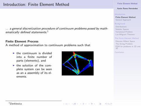
... a general discretization procedure of continuum problems posed by math-ematically defined statements.1
Finite Element ProcessA method of approximation to continuum problems such that
I the continuum is dividedinto a finite number ofparts (elements), and
I the solution of the com-plete system can be seenas an a assembly of its el-ements.
1Zienkiewicz
Finite Element Method
Aaron Romo Hernandez
Introduction
Finite Element Method
General Approach
Background
Distributions
Sobolev Spaces
Variational Problem
Lax-Milgram Theorem
The Finite Element Method
Discrete Hilbert Space
The String Problem
FEM for problems in 2D and3D
Conclusion
Index
IntroductionFinite Element MethodGeneral Approach
BackgroundDistributionsSobolev SpacesVariational ProblemLax-Milgram Theorem
The Finite Element MethodDiscrete Hilbert SpaceThe String ProblemFEM for problems in 2D and 3D
Conclusion
Finite Element Method
Aaron Romo Hernandez
Introduction
Finite Element Method
General Approach
Background
Distributions
Sobolev Spaces
Variational Problem
Lax-Milgram Theorem
The Finite Element Method
Discrete Hilbert Space
The String Problem
FEM for problems in 2D and3D
Conclusion
Introduction: General Approach
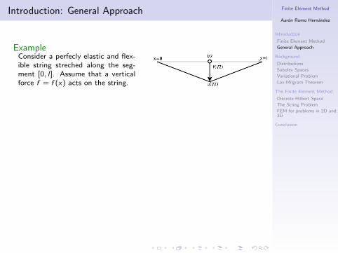
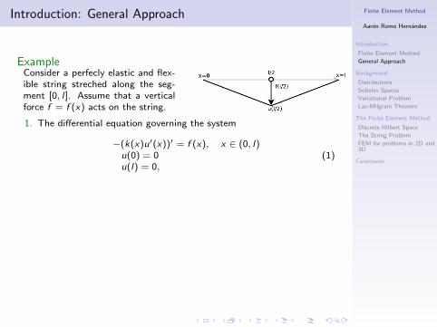
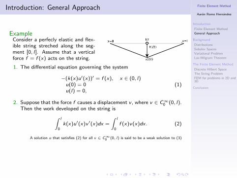
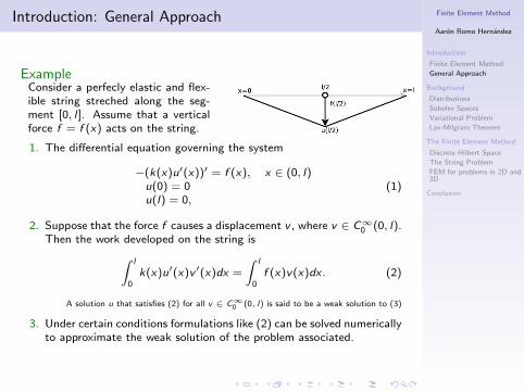
ExampleConsider a perfecly elastic and flex-ible string streched along the seg-ment [0, l ]. Assume that a verticalforce f = f (x) acts on the string.
1. The differential equation governing the system
−(k(x)u′(x))′ = f (x), x ∈ (0, l)u(0) = 0u(l) = 0,
(1)
2. Suppose that the force f causes a displacement v , where v ∈ C∞0 (0, l).Then the work developed on the string is∫ l
0k(x)u′(x)v ′(x)dx =
∫ l
0f (x)v(x)dx . (2)
A solution u that satisfies (2) for all v ∈ C∞0 (0, l) is said to be a weak solution to (3)
3. Under certain conditions formulations like (2) can be solved numericallyto approximate the weak solution of the problem associated.
Finite Element Method
Aaron Romo Hernandez
Introduction
Finite Element Method
General Approach
Background
Distributions
Sobolev Spaces
Variational Problem
Lax-Milgram Theorem
The Finite Element Method
Discrete Hilbert Space
The String Problem
FEM for problems in 2D and3D
Conclusion
Introduction: General Approach
ExampleConsider a perfecly elastic and flex-ible string streched along the seg-ment [0, l ]. Assume that a verticalforce f = f (x) acts on the string.
1. The differential equation governing the system
−(k(x)u′(x))′ = f (x), x ∈ (0, l)u(0) = 0u(l) = 0,
(1)
2. Suppose that the force f causes a displacement v , where v ∈ C∞0 (0, l).Then the work developed on the string is∫ l
0k(x)u′(x)v ′(x)dx =
∫ l
0f (x)v(x)dx . (2)
A solution u that satisfies (2) for all v ∈ C∞0 (0, l) is said to be a weak solution to (3)
3. Under certain conditions formulations like (2) can be solved numericallyto approximate the weak solution of the problem associated.
Finite Element Method
Aaron Romo Hernandez
Introduction
Finite Element Method
General Approach
Background
Distributions
Sobolev Spaces
Variational Problem
Lax-Milgram Theorem
The Finite Element Method
Discrete Hilbert Space
The String Problem
FEM for problems in 2D and3D
Conclusion
Index
IntroductionFinite Element MethodGeneral Approach
BackgroundDistributionsSobolev SpacesVariational ProblemLax-Milgram Theorem
The Finite Element MethodDiscrete Hilbert SpaceThe String ProblemFEM for problems in 2D and 3D
Conclusion
Finite Element Method
Aaron Romo Hernandez
Introduction
Finite Element Method
General Approach
Background
Distributions
Sobolev Spaces
Variational Problem
Lax-Milgram Theorem
The Finite Element Method
Discrete Hilbert Space
The String Problem
FEM for problems in 2D and3D
Conclusion
Background: Distributions I
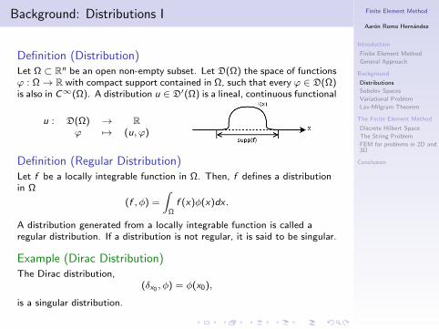
Definition (Distribution)Let Ω ⊂ Rn be an open non-empty subset. Let D(Ω) the space of functionsϕ : Ω→ R with compact support contained in Ω, such that every ϕ ∈ D(Ω)is also in C∞(Ω). A distribution u ∈ D′(Ω) is a lineal, continuous functional
u : D(Ω) → Rϕ 7→ (u, ϕ)
Definition (Regular Distribution)Let f be a locally integrable function in Ω. Then, f defines a distributionin Ω
(f , φ) =
∫Ω
f (x)φ(x)dx .
A distribution generated from a locally integrable function is called aregular distribution. If a distribution is not regular, it is said to be singular.
Example (Dirac Distribution)The Dirac distribution,
(δx0 , φ) = φ(x0),
is a singular distribution.
Finite Element Method
Aaron Romo Hernandez
Introduction
Finite Element Method
General Approach
Background
Distributions
Sobolev Spaces
Variational Problem
Lax-Milgram Theorem
The Finite Element Method
Discrete Hilbert Space
The String Problem
FEM for problems in 2D and3D
Conclusion
Background: Distributions II
Definition (Partial Differential Operator)Let Ω ∈ Rn be an open non-empty subset. Let ϕ ∈ C k (Ω), and α ∈ Nn,|α| ≤ k. The general partial differential operator is defined as
∂αϕ =∂|α|ϕ
∂xα11 · · · ∂xαn
n, |α| = α1 + . . .+ αn
Definition (Distributional Derivative)Let α ∈ N be a multi-index given. Let u ∈ D′(Ω) be a distribution. Wedefine de distributional derivative of u as a distribution
∂αu : D(Ω) → Rϕ 7→ (∂αu, ϕ)
where (∂αu, ϕ) = (−1)|α|(u, ∂αϕ)
Definition (Distributional Product)Let f ∈ C∞(Ω) and u ∈ D′(Ω). The distribution fu is defined by
(fu, ϕ) = (u, f ϕ) ∀ϕ ∈ D(Ω).
Finite Element Method
Aaron Romo Hernandez
Introduction
Finite Element Method
General Approach
Background
Distributions
Sobolev Spaces
Variational Problem
Lax-Milgram Theorem
The Finite Element Method
Discrete Hilbert Space
The String Problem
FEM for problems in 2D and3D
Conclusion
Index
IntroductionFinite Element MethodGeneral Approach
BackgroundDistributionsSobolev SpacesVariational ProblemLax-Milgram Theorem
The Finite Element MethodDiscrete Hilbert SpaceThe String ProblemFEM for problems in 2D and 3D
Conclusion
Finite Element Method
Aaron Romo Hernandez
Introduction
Finite Element Method
General Approach
Background
Distributions
Sobolev Spaces
Variational Problem
Lax-Milgram Theorem
The Finite Element Method
Discrete Hilbert Space
The String Problem
FEM for problems in 2D and3D
Conclusion
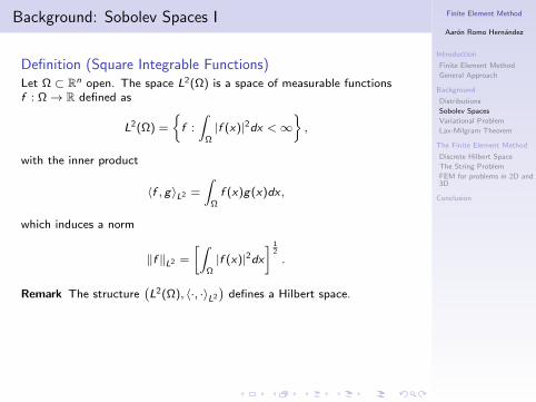
Background: Sobolev Spaces I
Definition (Square Integrable Functions)Let Ω ⊂ Rn open. The space L2(Ω) is a space of measurable functionsf : Ω→ R defined as
L2(Ω) =
f :
∫Ω|f (x)|2dx <∞
,
with the inner product
〈f , g〉L2 =
∫Ω
f (x)g(x)dx ,
which induces a norm
‖f ‖L2 =
[∫Ω|f (x)|2dx
] 12
.
Remark The structure(L2(Ω), 〈·, ·〉L2
)defines a Hilbert space.
Finite Element Method
Aaron Romo Hernandez
Introduction
Finite Element Method
General Approach
Background
Distributions
Sobolev Spaces
Variational Problem
Lax-Milgram Theorem
The Finite Element Method
Discrete Hilbert Space
The String Problem
FEM for problems in 2D and3D
Conclusion
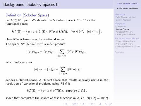
Background: Sobolev Spaces II
Definition (Sobolev Space)Let Ω ⊂ Rn open. We denote the Sobolev Space Hm in Ω as thefunctional space
Hm(Ω) =
u : u ∈ L2(Ω), ∂αu ∈ L2(Ω), ∀α ∈ Nb, |α| ≤ m.
Here ∂αu is taken in a distributional sense.
The space Hm defined with a inner product
〈u, v〉Hm = 〈u, v〉L2 +∑|α|≤m
〈∂αu, ∂αv〉L2 ,
which induces a norm
‖u‖Hm = ‖u‖L2 +∑|α|≤m
‖∂αu‖L2 ,
defines a Hilbert space. A Hilbert space that results specially useful in theresolution of variational problems using FEM is
Hm0 (Ω) = u : u ∈ Hm(Ω), supp(u) ⊂ Ω ,
space that completes the spaces of test functions in Ω, i.e. Hm0 (Ω) = D(Ω)
Finite Element Method
Aaron Romo Hernandez
Introduction
Finite Element Method
General Approach
Background
Distributions
Sobolev Spaces
Variational Problem
Lax-Milgram Theorem
The Finite Element Method
Discrete Hilbert Space
The String Problem
FEM for problems in 2D and3D
Conclusion
Index
IntroductionFinite Element MethodGeneral Approach
BackgroundDistributionsSobolev SpacesVariational ProblemLax-Milgram Theorem
The Finite Element MethodDiscrete Hilbert SpaceThe String ProblemFEM for problems in 2D and 3D
Conclusion
Finite Element Method
Aaron Romo Hernandez
Introduction
Finite Element Method
General Approach
Background
Distributions
Sobolev Spaces
Variational Problem
Lax-Milgram Theorem
The Finite Element Method
Discrete Hilbert Space
The String Problem
FEM for problems in 2D and3D
Conclusion
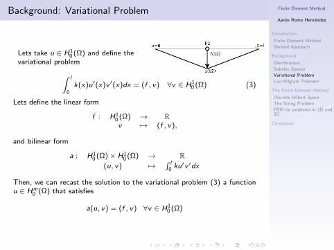
Background: Variational Problem
Lets take u ∈ H10 (Ω) and define the
variational problem∫ l
0k(x)u′(x)v ′(x)dx = (f , v) ∀v ∈ H1
0 (Ω) (3)
Lets define the linear form
f : H10 (Ω) → Rv 7→ (f , v),
and bilinear form
a : H10 (Ω)× H1
0 (Ω) → R(u, v) 7→
∫ l0 ku′v ′dx
Then, we can recast the solution to the variational problem (3) a functionu ∈ Hm
0 (Ω) that satisfies
a(u, v) = (f , v) ∀v ∈ H10 (Ω)
Finite Element Method
Aaron Romo Hernandez
Introduction
Finite Element Method
General Approach
Background
Distributions
Sobolev Spaces
Variational Problem
Lax-Milgram Theorem
The Finite Element Method
Discrete Hilbert Space
The String Problem
FEM for problems in 2D and3D
Conclusion
Index
IntroductionFinite Element MethodGeneral Approach
BackgroundDistributionsSobolev SpacesVariational ProblemLax-Milgram Theorem
The Finite Element MethodDiscrete Hilbert SpaceThe String ProblemFEM for problems in 2D and 3D
Conclusion
Finite Element Method
Aaron Romo Hernandez
Introduction
Finite Element Method
General Approach
Background
Distributions
Sobolev Spaces
Variational Problem
Lax-Milgram Theorem
The Finite Element Method
Discrete Hilbert Space
The String Problem
FEM for problems in 2D and3D
Conclusion
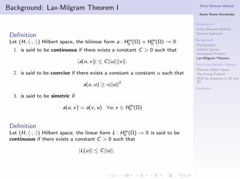
Background: Lax-Milgram Theorem I
DefinitionLet (H, 〈·, ·〉) Hilbert space, the bilinear form a : Hm
0 (Ω)× Hm0 (Ω)→ R
1. is said to be continuous if there exists a constant C > 0 such that
|a(u, v)| ≤ C‖u‖‖v‖.
2. is said to be coercive if there exists a constant a constant α such that
a(u, u) ≥ α‖u‖2
3. is said to be simetric if
a(u, v) = a(v , u) ∀u, v ∈ Hm0 (Ω)
DefinitionLet (H, 〈·, ·〉) Hilbert space, the linear form L : Hm
0 (Ω)→ R is said to becontinuous if there exists a constant C > 0 such that
|L(u)| ≤ C‖u‖.
Finite Element Method
Aaron Romo Hernandez
Introduction
Finite Element Method
General Approach
Background
Distributions
Sobolev Spaces
Variational Problem
Lax-Milgram Theorem
The Finite Element Method
Discrete Hilbert Space
The String Problem
FEM for problems in 2D and3D
Conclusion
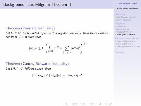
Background: Lax-Milgram Theorem II
Theorem (Poincare Inequality)Let Ω ⊂ Rn be bounded, open with a regular boundary, then there exists aconstant C > 0 such that
‖u‖Hm ≤ C
∫∂Ω|u|2 +
∑|α|≤m
|∂αu|2 1
2
Theorem (Cauchy-Schwartz Inequality)Let (H, 〈·, ·〉) Hilbert space, then
| 〈u, v〉H | ≤ ‖u‖H‖v‖Hm ∀u, v ∈ H
Finite Element Method
Aaron Romo Hernandez
Introduction
Finite Element Method
General Approach
Background
Distributions
Sobolev Spaces
Variational Problem
Lax-Milgram Theorem
The Finite Element Method
Discrete Hilbert Space
The String Problem
FEM for problems in 2D and3D
Conclusion
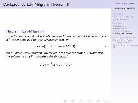
Background: Lax-Milgram Theorem III
Theorem (Lax-Milgram)If the bilinear form a(·, ·) is continuous and coercive, and if the linear formL(·) is continuous, then the variational problem
a(u, v) = L(v) ∀v ∈ Hm0 (Ω) (4)
has a unique weak solution. Moreover if the bilinear form a is symmetricthe solution u to (5) minimizes the functional
J(v) =1
2a(v , v)− L(v)
Finite Element Method
Aaron Romo Hernandez
Introduction
Finite Element Method
General Approach
Background
Distributions
Sobolev Spaces
Variational Problem
Lax-Milgram Theorem
The Finite Element Method
Discrete Hilbert Space
The String Problem
FEM for problems in 2D and3D
Conclusion
Index
IntroductionFinite Element MethodGeneral Approach
BackgroundDistributionsSobolev SpacesVariational ProblemLax-Milgram Theorem
The Finite Element MethodDiscrete Hilbert SpaceThe String ProblemFEM for problems in 2D and 3D
Conclusion
Finite Element Method
Aaron Romo Hernandez
Introduction
Finite Element Method
General Approach
Background
Distributions
Sobolev Spaces
Variational Problem
Lax-Milgram Theorem
The Finite Element Method
Discrete Hilbert Space
The String Problem
FEM for problems in 2D and3D
Conclusion
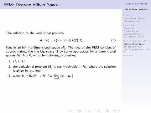
FEM: Discrete Hilbert Space
The solution to the variational problem
a(u, v) = L(v) ∀v ∈ Hm0 (Ω) (5)
lives in an infinite dimensional space H10 . The idea of the FEM consists of
approximating the the big space H by some appropiate finite-dimensionalspaces Hh, h > 0, with the following properties:
1. Hh ⊆ H,
2. the variational problem (5) is easily solvable in Hh, where the solutionis given by uh, and
3. when h→ 0, Hh → H, i.e. limx→0‖u − uh‖
Finite Element Method
Aaron Romo Hernandez
Introduction
Finite Element Method
General Approach
Background
Distributions
Sobolev Spaces
Variational Problem
Lax-Milgram Theorem
The Finite Element Method
Discrete Hilbert Space
The String Problem
FEM for problems in 2D and3D
Conclusion
Index
IntroductionFinite Element MethodGeneral Approach
BackgroundDistributionsSobolev SpacesVariational ProblemLax-Milgram Theorem
The Finite Element MethodDiscrete Hilbert SpaceThe String ProblemFEM for problems in 2D and 3D
Conclusion
Finite Element Method
Aaron Romo Hernandez
Introduction
Finite Element Method
General Approach
Background
Distributions
Sobolev Spaces
Variational Problem
Lax-Milgram Theorem
The Finite Element Method
Discrete Hilbert Space
The String Problem
FEM for problems in 2D and3D
Conclusion
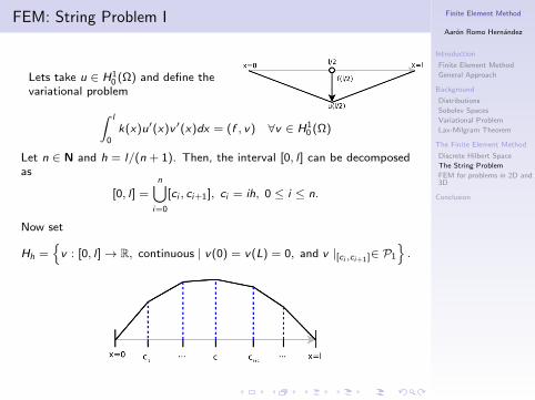
FEM: String Problem I
Lets take u ∈ H10 (Ω) and define the
variational problem∫ l
0k(x)u′(x)v ′(x)dx = (f , v) ∀v ∈ H1
0 (Ω)
Let n ∈ N and h = l/(n + 1). Then, the interval [0, l ] can be decomposedas
[0, l ] =n⋃
i=0
[ci , ci+1], ci = ih, 0 ≤ i ≤ n.
Now set
Hh =
v : [0, l ]→ R, continuous | v(0) = v(L) = 0, and v |[ci ,ci+1]∈ P1
.
Finite Element Method
Aaron Romo Hernandez
Introduction
Finite Element Method
General Approach
Background
Distributions
Sobolev Spaces
Variational Problem
Lax-Milgram Theorem
The Finite Element Method
Discrete Hilbert Space
The String Problem
FEM for problems in 2D and3D
Conclusion
FEM: String Problem II
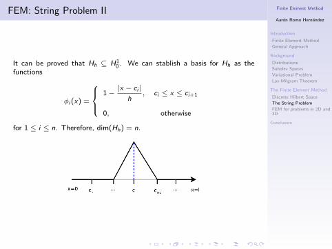
It can be proved that Hh ⊆ H10 . We can stablish a basis for Hh as the
functions
φi (x) =
1−|x − ci |
h, ci ≤ x ≤ ci+1
0, otherwise
for 1 ≤ i ≤ n. Therefore, dim(Hh) = n.
Finite Element Method
Aaron Romo Hernandez
Introduction
Finite Element Method
General Approach
Background
Distributions
Sobolev Spaces
Variational Problem
Lax-Milgram Theorem
The Finite Element Method
Discrete Hilbert Space
The String Problem
FEM for problems in 2D and3D
Conclusion
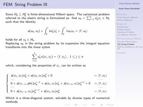
FEM: String Problem III
Since Hh ⊆ H10 is finite-dimensional Hilbert space. The variational problem
referred to the elastic string is formulated as: find uh =∑n
i=1 uihφi ∈ Hh
such that the identity
a(uh, vh) +∫ l
0ku′hv ′h +
∫ l
0λuhvh = 〈f , vh〉
holds for all vh ∈ Hh.Replacing uh in the string problem by its expansion the integral equationtransforms into the linear sytem
n∑i=1
uihx(φi , φj ) =
⟨f , φj
⟩, 1 ≤ j ≤ n
which, considering the properties of φi , can be written as
a(φ1, φ1)u1
h + a(φ2, φ1)u2h + 0 = 〈f , φ1〉
· · · · · ·0 + a(φi−1, phii )ui−1
h + a(φi , φi )uih + a(φi+1, φi )ui+1
h + 0 = 〈f , φi 〉· · · · · ·0 + a(φn−1, φn)un−1
h + a(φn, φn)unh = 〈f , φi 〉
Which is a three-diagonal system, solvable by diverse types of numericalmethods.
Finite Element Method
Aaron Romo Hernandez
Introduction
Finite Element Method
General Approach
Background
Distributions
Sobolev Spaces
Variational Problem
Lax-Milgram Theorem
The Finite Element Method
Discrete Hilbert Space
The String Problem
FEM for problems in 2D and3D
Conclusion
Index
IntroductionFinite Element MethodGeneral Approach
BackgroundDistributionsSobolev SpacesVariational ProblemLax-Milgram Theorem
The Finite Element MethodDiscrete Hilbert SpaceThe String ProblemFEM for problems in 2D and 3D
Conclusion
Finite Element Method
Aaron Romo Hernandez
Introduction
Finite Element Method
General Approach
Background
Distributions
Sobolev Spaces
Variational Problem
Lax-Milgram Theorem
The Finite Element Method
Discrete Hilbert Space
The String Problem
FEM for problems in 2D and3D
Conclusion
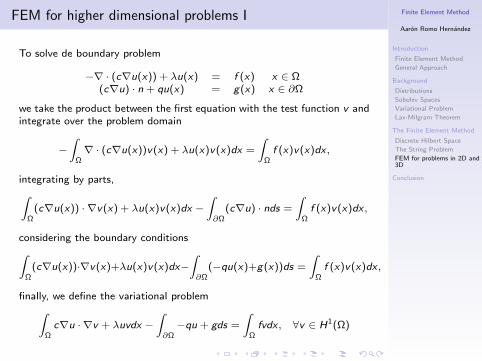
FEM for higher dimensional problems I
To solve de boundary problem
−∇ · (c∇u(x)) + λu(x) = f (x) x ∈ Ω(c∇u) · n + qu(x) = g(x) x ∈ ∂Ω
we take the product between the first equation with the test function v andintegrate over the problem domain
−∫
Ω∇ · (c∇u(x))v(x) + λu(x)v(x)dx =
∫Ω
f (x)v(x)dx ,
integrating by parts,∫Ω
(c∇u(x)) · ∇v(x) + λu(x)v(x)dx −∫∂Ω
(c∇u) · nds =
∫Ω
f (x)v(x)dx ,
considering the boundary conditions∫Ω
(c∇u(x))·∇v(x)+λu(x)v(x)dx−∫∂Ω
(−qu(x)+g(x))ds =
∫Ω
f (x)v(x)dx ,
finally, we define the variational problem∫Ω
c∇u · ∇v + λuvdx −∫∂Ω−qu + gds =
∫Ω
fvdx , ∀v ∈ H1(Ω)
Finite Element Method
Aaron Romo Hernandez
Introduction
Finite Element Method
General Approach
Background
Distributions
Sobolev Spaces
Variational Problem
Lax-Milgram Theorem
The Finite Element Method
Discrete Hilbert Space
The String Problem
FEM for problems in 2D and3D
Conclusion
FEM for higher dimensional problems II
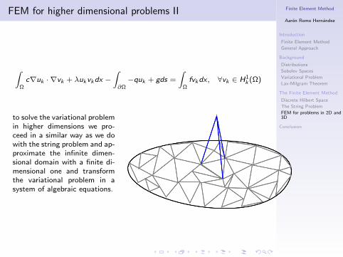
∫Ω
c∇uk · ∇vk + λuk vk dx −∫∂Ω−quk + gds =
∫Ω
fvk dx , ∀vk ∈ H1k (Ω)
to solve the variational problemin higher dimensions we pro-ceed in a similar way as we dowith the string problem and ap-proximate the infinite dimen-sional domain with a finite di-mensional one and transformthe variational problem in asystem of algebraic equations.
Finite Element Method
Aaron Romo Hernandez
Introduction
Finite Element Method
General Approach
Background
Distributions
Sobolev Spaces
Variational Problem
Lax-Milgram Theorem
The Finite Element Method
Discrete Hilbert Space
The String Problem
FEM for problems in 2D and3D
Conclusion
Conclusion
The Finite Element Method provides a useful tool for solving boundary valueproblems. Using FEM we are able to transform a hard PDE problem into asystem of linear equations, or a system of ODEs, which is solved relativelyeasy. However, we have to be careful defining the variational problem andwe must care about when the weak solution converges to the solution ofthe original problem.
Finite Element Method
Aaron Romo Hernandez
Introduction
Finite Element Method
General Approach
Background
Distributions
Sobolev Spaces
Variational Problem
Lax-Milgram Theorem
The Finite Element Method
Discrete Hilbert Space
The String Problem
FEM for problems in 2D and3D
Conclusion
References