FINITE ELEMENT EXTERIOR CALCULUS: FROM HODGE …arnold/papers/bulletin.pdfFINITE ELEMENT EXTERIOR...
74
This is a free offprint provided to the author by the publisher. Copyright restrictions may apply. BULLETIN (New Series) OF THE AMERICAN MATHEMATICAL SOCIETY Volume 47, Number 2, April 2010, Pages 281–354 S 0273-0979(10)01278-4 Article electronically published on January 25, 2010 FINITE ELEMENT EXTERIOR CALCULUS: FROM HODGE THEORY TO NUMERICAL STABILITY DOUGLAS N. ARNOLD, RICHARD S. FALK, AND RAGNAR WINTHER Abstract. This article reports on the confluence of two streams of research, one emanating from the fields of numerical analysis and scientific computa- tion, the other from topology and geometry. In it we consider the numerical discretization of partial differential equations that are related to differential complexes so that de Rham cohomology and Hodge theory are key tools for exploring the well-posedness of the continuous problem. The discretization methods we consider are finite element methods, in which a variational or weak formulation of the PDE problem is approximated by restricting the trial subspace to an appropriately constructed piecewise polynomial subspace. Af- ter a brief introduction to finite element methods, we develop an abstract Hilbert space framework for analyzing the stability and convergence of such discretizations. In this framework, the differential complex is represented by a complex of Hilbert spaces, and stability is obtained by transferring Hodge- theoretic structures that ensure well-posedness of the continuous problem from the continuous level to the discrete. We show stable discretization is achieved if the finite element spaces satisfy two hypotheses: they can be arranged into a subcomplex of this Hilbert complex, and there exists a bounded cochain pro- jection from that complex to the subcomplex. In the next part of the paper, we consider the most canonical example of the abstract theory, in which the Hilbert complex is the de Rham complex of a domain in Euclidean space. We use the Koszul complex to construct two families of finite element differential forms, show that these can be arranged in subcomplexes of the de Rham com- plex in numerous ways, and for each construct a bounded cochain projection. The abstract theory therefore applies to give the stability and convergence of finite element approximations of the Hodge Laplacian. Other applications are considered as well, especially the elasticity complex and its application to the equations of elasticity. Background material is included to make the presentation self-contained for a variety of readers. 1. Introduction Numerical algorithms for the solution of partial differential equations are an es- sential tool of the modern world. They are applied in countless ways every day in problems as varied as the design of aircraft, prediction of climate, development of cardiac devices, and modeling of the financial system. Science, engineering, and Received by the editors June 23, 2009, and, in revised form, August 12, 2009. 2000 Mathematics Subject Classification. Primary: 65N30, 58A14. Key words and phrases. Finite element exterior calculus, exterior calculus, de Rham cohomol- ogy, Hodge theory, Hodge Laplacian, mixed finite elements. The work of the first author was supported in part by NSF grant DMS-0713568. The work of the second author was supported in part by NSF grant DMS-0609755. The work of the third author was supported by the Norwegian Research Council. c 2010 American Mathematical Society 281
Transcript of FINITE ELEMENT EXTERIOR CALCULUS: FROM HODGE …arnold/papers/bulletin.pdfFINITE ELEMENT EXTERIOR...

This is a free offprint provided to the author by the publisher. Copyright restrictions may apply.
BULLETIN (New Series) OF THEAMERICAN MATHEMATICAL SOCIETYVolume 47, Number 2, April 2010, Pages 281–354S 0273-0979(10)01278-4Article electronically published on January 25, 2010
FINITE ELEMENT EXTERIOR CALCULUS:
FROM HODGE THEORY TO NUMERICAL STABILITY
DOUGLAS N. ARNOLD, RICHARD S. FALK, AND RAGNAR WINTHER
Abstract. This article reports on the confluence of two streams of research,one emanating from the fields of numerical analysis and scientific computa-tion, the other from topology and geometry. In it we consider the numericaldiscretization of partial differential equations that are related to differentialcomplexes so that de Rham cohomology and Hodge theory are key tools forexploring the well-posedness of the continuous problem. The discretizationmethods we consider are finite element methods, in which a variational orweak formulation of the PDE problem is approximated by restricting the trialsubspace to an appropriately constructed piecewise polynomial subspace. Af-ter a brief introduction to finite element methods, we develop an abstractHilbert space framework for analyzing the stability and convergence of suchdiscretizations. In this framework, the differential complex is represented bya complex of Hilbert spaces, and stability is obtained by transferring Hodge-theoretic structures that ensure well-posedness of the continuous problem fromthe continuous level to the discrete. We show stable discretization is achievedif the finite element spaces satisfy two hypotheses: they can be arranged into asubcomplex of this Hilbert complex, and there exists a bounded cochain pro-jection from that complex to the subcomplex. In the next part of the paper,we consider the most canonical example of the abstract theory, in which theHilbert complex is the de Rham complex of a domain in Euclidean space. Weuse the Koszul complex to construct two families of finite element differentialforms, show that these can be arranged in subcomplexes of the de Rham com-
plex in numerous ways, and for each construct a bounded cochain projection.The abstract theory therefore applies to give the stability and convergenceof finite element approximations of the Hodge Laplacian. Other applicationsare considered as well, especially the elasticity complex and its applicationto the equations of elasticity. Background material is included to make thepresentation self-contained for a variety of readers.
1. Introduction
Numerical algorithms for the solution of partial differential equations are an es-sential tool of the modern world. They are applied in countless ways every day inproblems as varied as the design of aircraft, prediction of climate, development ofcardiac devices, and modeling of the financial system. Science, engineering, and
Received by the editors June 23, 2009, and, in revised form, August 12, 2009.2000 Mathematics Subject Classification. Primary: 65N30, 58A14.Key words and phrases. Finite element exterior calculus, exterior calculus, de Rham cohomol-
ogy, Hodge theory, Hodge Laplacian, mixed finite elements.The work of the first author was supported in part by NSF grant DMS-0713568.The work of the second author was supported in part by NSF grant DMS-0609755.The work of the third author was supported by the Norwegian Research Council.
c©2010 American Mathematical Society
281
This is a free offprint provided to the author by the publisher. Copyright restrictions may apply.
282 D. N. ARNOLD, R. S. FALK, AND RAGNAR WINTHER
technology depend not only on efficient and accurate algorithms for approximatingthe solutions of a vast and diverse array of differential equations which arise inapplications, but also on mathematical analysis of the behavior of computed solu-tions, in order to validate the computations, determine the ranges of applicability,compare different algorithms, and point the way to improved numerical methods.Given a partial differential equation (PDE) problem, a numerical algorithm approx-imates the solution by the solution of a finite-dimensional problem which can beimplemented and solved on a computer. This discretization depends on a parame-ter (representing, for example, a grid spacing, mesh size, or time step) which canbe adjusted to obtain a more accurate approximate solution, at the cost of a largerfinite-dimensional problem. The mathematical analysis of the algorithm aims todescribe the relationship between the true solution and the numerical solution asthe discretization parameter is varied. For example, at its most basic, the theoryattempts to establish convergence of the discrete solution to the true solution in anappropriate sense as the discretization parameter tends to zero.
Underlying the analysis of numerical methods for PDEs is the realization thatconvergence depends on consistency and stability of the discretization. Consistency,whose precise definition depends on the particular PDE problem and the type ofnumerical method, aims to capture the idea that the operators and data defining thediscrete problem are appropriately close to those of the true problem for small valuesof the discretization parameter. The essence of stability is that the discrete problemis well-posed, uniformly with respect to the discretization parameter. Like well-posedness of the PDE problem itself, stability can be very elusive. One might thinkthat well-posedness of the PDE problem, which means invertibility of the operator,together with consistency of the discretization, would imply invertibility of thediscrete operator, since invertible operators between a pair of Banach spaces form anopen set in the norm topology. But this reasoning is bogus. Consistency is not andcannot be defined to mean norm convergence of the discrete operators to the PDEoperator, since the PDE operator, being an invertible operator between infinite-dimensional spaces, is not compact and so is not the norm limit of finite-dimensionaloperators. In fact, in the first part of the preceding century, a fundamental, andinitially unexpected, realization was made: that a consistent discretization of awell-posed problem need not be stable [36, 86, 29]. Only for very special classesof problems and algorithms does well-posedness at the continuous level transfer tostability at the discrete level. In other situations, the development and analysisof stable, consistent algorithms can be a challenging problem, to which a widearray of mathematical techniques has been applied, just as for establishing thewell-posedness of PDEs.
In this paper we will consider PDEs that are related to differential complexes,for which de Rham cohomology and Hodge theory are key tools for exploring thewell-posedness of the continuous problem. These are linear elliptic PDEs, but theyare a fundamental component of problems arising in many mathematical models,including parabolic, hyperbolic, and nonlinear problems. The finite element exteriorcalculus, which we develop here, is a theory which was developed to capture thekey structures of de Rham cohomology and Hodge theory at the discrete level andto relate the discrete and continuous structures, in order to obtain stable finiteelement discretizations.
This is a free offprint provided to the author by the publisher. Copyright restrictions may apply.
FINITE ELEMENT EXTERIOR CALCULUS 283
1.1. The finite element method. The finite element method, whose develop-ment as an approach to the computer solution of PDEs began over 50 years agoand is still flourishing today, has proven to be one of the most important tech-nologies in numerical PDEs. Finite elements not only provide a methodology todevelop numerical algorithms for many different problems, but also a mathematicalframework in which to explore their behavior. They are based on a weak or varia-tional form of the PDE problem, and they fall into the class of Galerkin methods,in which the trial space for the weak formulation is replaced by a finite-dimensionalsubspace to obtain the discrete problem. For a finite element method, this subspaceis a space of piecewise polynomials defined by specifying three things: a simplicialdecomposition of the domain, and, for each simplex, a space of polynomials calledthe shape functions, and a set of degrees of freedom for the shape functions, i.e., abasis for their dual space, with each degree of freedom associated to a face of somedimension of the simplex. This allows for efficient implementation of the globalpiecewise polynomial subspace, with the degrees of freedom determining the degreeof interelement continuity.
For readers unfamilar with the finite element method, we introduce some basicideas by considering the approximation of the simplest two-point boundary valueproblem
(1) −u′′(x) = f(x), −1 < x < 1, u(−1) = u(1) = 0.
Weak solutions to this problem are sought in the Sobolev spaceH1(−1, 1) consistingof functions in L2(−1, 1) whose first derivatives also belong to L2(−1, 1). Indeed,the solution u can be characterized as the minimizer of the energy functional
(2) J(u) :=1
2
∫ 1
−1
|u′(x)|2 dx−∫ 1
−1
f(x)u(x) dx
over the space H1(−1, 1) (which consists of H1(−1, 1) functions vanishing at ±1),
or, equivalently, as the solution of the weak problem: Find u ∈ H1(−1, 1) such that
(3)
∫ 1
−1
u′(x)v′(x) dx =
∫ 1
−1
f(x)v(x) dx, v ∈ H1(−1, 1).
It is easily seen by integrating by parts that a smooth solution of the boundary valueproblem satisfies the weak formulation and that a solution of the weak formulationwhich possesses appropriate smoothness will be a solution of the boundary valueproblem.
Letting Vh denote a finite-dimensional subspace of H1(−1, 1), called the trialspace, we may define an approximate solution uh ∈ Vh as the minimizer of thefunctional J over the trial space (the classical Ritz method), or, equivalently byGalerkin’s method, in which uh ∈ Vh is determined by requiring that the variationgiven in the weak problem hold only for functions in Vh, i.e., by the equations∫ 1
−1
u′h(x) v
′(x) dx =
∫ 1
−1
f(x) v(x) dx, v ∈ Vh.
By choosing a basis for the trial space Vh, the Galerkin method reduces to a linearsystem of algebraic equations for the coefficients of the expansion of uh in terms
of the basis functions. More specifically, if we write uh =∑M
j=1 cjφj , where thefunctions φj form a basis for the trial space, then the Galerkin equations hold ifand only if Ac = b, where the coefficient matrix of the linear system is given by
This is a free offprint provided to the author by the publisher. Copyright restrictions may apply.
284 D. N. ARNOLD, R. S. FALK, AND RAGNAR WINTHER
Aij =∫ 1
−1φ′j φ
′i dx and bi =
∫ 1
−1fφi dx. Since this is a square system of linear
equations, it is nonsingular if and only if the only solution for f = 0 is uh = 0. Thisfollows immediately by choosing v = uh.
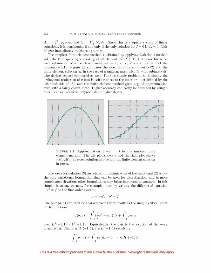
The simplest finite element method is obtained by applying Galerkin’s methodwith the trial space Vh consisting of all elements of H1(−1, 1) that are linear oneach subinterval of some chosen mesh −1 = x0 < x1 < · · · < xN = 1 of thedomain (−1, 1). Figure 1.1 compares the exact solution u = cos(πx/2) and thefinite element solution uh in the case of a uniform mesh with N = 14 subintervals.The derivatives are compared as well. For this simple problem, uh is simply theorthogonal projection of u into Vh with respect to the inner product defined by theleft-hand side of (3), and the finite element method gives a good approximationeven with a fairly coarse mesh. Higher accuracy can easily be obtained by using afiner mesh or piecewise polynomials of higher degree.
Figure 1.1. Approximation of −u′′ = f by the simplest finiteelement method. The left plot shows u and the right plot shows−u′, with the exact solution in blue and the finite element solutionin green.
The weak formulation (3) associated to minimization of the functional (2) is notthe only variational formulation that can be used for discretization, and in morecomplicated situations other formulations may bring important advantages. In thissimple situation, we may, for example, start by writing the differential equation−u′′ = f as the first-order system
σ = −u′, σ′ = f.
The pair (σ, u) can then be characterized variationally as the unique critical pointof the functional
I(σ, u) =
∫ 1
−1
(1
2σ2 − uσ′) dx+
∫ 1
−1
fu dx
over H1(−1, 1) × L2(−1, 1). Equivalently, the pair is the solution of the weakformulation: Find σ ∈ H1(−1, 1), u ∈ L2(−1, 1) satisfying∫ 1
−1
στ dx−∫ 1
−1
uτ ′ dx = 0, τ ∈ H1(−1, 1),

This is a free offprint provided to the author by the publisher. Copyright restrictions may apply.
FINITE ELEMENT EXTERIOR CALCULUS 285∫ 1
−1
σ′v dx =
∫ 1
−1
fv dx, v ∈ L2(−1, 1).
This is called a mixed formulation of the boundary value problem. Note that for themixed formulation, the Dirichlet boundary condition is implied by the formulation,as can be seen by integration by parts. Note also that in this case the solution is asaddle point of the functional I, not an extremum: I(σ, v) ≤ I(σ, u) ≤ I(τ, u) forτ ∈ H1(−1, 1), v ∈ L2(−1, 1).
Although the mixed formulation is perfectly well-posed, it may easily lead to adiscretization which is not. If we apply Galerkin’s method with a simple choice oftrial subspaces Σh ⊂ H1(−1, 1) and Vh ⊂ L2(−1, 1), we obtain a finite-dimensionallinear system, which, however, may be singular, or may become increasingly un-stable as the mesh is refined. This concept will be formalized and explored in thenext section, but the result of such instability is clearly visible in simple compu-tations. For example, the choice of continuous piecewise linear functions for bothΣh and Vh leads to a singular linear system. The choice of continuous piecewiselinear functions for Σh and piecewise constants for Vh leads to stable discretizationand good accuracy. However choosing piecewise quadratics for Σh and piecewiseconstants for Vh gives a nonsingular system but unstable approximation (see [25]for further discussion of this example). The dramatic difference between the stableand unstable methods can be seen in Figure 1.2.
Figure 1.2. Approximation of the mixed formulation for−u′′ = fin one dimension with two choices of elements, piecewise constantsfor u and piecewise linears for σ (a stable method, shown in green),or piecewise constants for u and piecewise quadratics for σ (unsta-ble, shown in red). The left plot shows u and the right plot showsσ, with the exact solution in blue. (In the right plot, the blue curveessentially coincides with the green curve and hence is not visible.)
In one dimension, finding stable pairs of finite-dimensional subspaces for themixed formulation of the two-point boundary value problem is easy. For any integerr ≥ 1, the combination of continuous piecewise polynomials of degree at most r forσ and arbitrary piecewise polynomials of degree at most r−1 for u is stable as can beverified via elementary means (and which can be viewed as a very simple applicationof the theory presented in this paper). In higher dimensions, the problem of findingstable combinations of elements is considerably more complicated. This is discussed

This is a free offprint provided to the author by the publisher. Copyright restrictions may apply.
286 D. N. ARNOLD, R. S. FALK, AND RAGNAR WINTHER
in Section 2.3.1 below. In particular, we shall see that the choice of continuouspiecewise linear functions for σ and piecewise constant functions for u is not stablein more than one dimension. However, stable element choices are known for thisproblem and again may be viewed as a simple application of the finite elementexterior calculus developed in this paper.
1.2. The contents of this paper. The brief introduction to the finite elementmethod just given will be continued in Section 2. In particular, there we formalizethe notions of consistency and stability and establish their relation to convergence.We shall also give several more computational examples. While seemingly simple,some of these examples may be surprising even to specialists, and they illustratethe difficulty in obtaining good methods and the need for a theoretical frameworkin which to understand such behaviors.
Like the theory of weak solutions of PDEs, the theory of finite element meth-ods is based on functional analysis and takes its most natural form in a Hilbertspace setting. In Section 3 of this paper, we develop an abstract Hilbert spaceframework, which captures key elements of Hodge theory and which can be usedto explore the stability of finite element methods. The most basic object in thisframework is a cochain complex of Hilbert spaces, referred to as a Hilbert complex.Function spaces of such complexes will occur in the weak formulations of the PDEproblems we consider, and the differentials will be differential operators enteringinto the PDE problem. The most canonical example of a Hilbert complex is the L2
de Rham complex of a Riemannian manifold, but it is a far more general object withother important realizations. For example, it allows for the definition of spaces ofharmonic forms and the proof that they are isomorphic to the cohomology groups.A Hilbert complex includes enough structure to define an abstract Hodge Lapla-cian, defined from a variational problem with a saddle point structure. However,for these problems to be well-posed, we need the additional property of a closedHilbert complex, i.e., that the range of the differentials are closed.
In this framework, the finite element spaces used to compute approximate so-lutions are represented by finite-dimensional subspaces of the spaces in the closedHilbert complex. We identify two key properties of these subspaces: first, theyshould combine to form a subcomplex of the Hilbert complex, and, second, thereshould exist a bounded cochain projection from the Hilbert complex to this sub-complex. Under these hypotheses and a minor consistency condition, it is easy toshow that the subcomplex inherits the cohomology of the true complex, i.e., thatthe cochain projections induce an isomorphism from the space of harmonic forms tothe space of discrete harmonic forms, and to get an error estimate on the differencebetween a harmonic form and its discrete counterpart. In the applications, this willbe crucial for stable approximation of the PDEs. In fact, a main theme of finiteelement exterior calculus is that the same two assumptions, the subcomplex prop-erty and the existence of a bounded cochain projection, are the natural hypothesesto establish the stability of the corresponding discrete Hodge Laplacian, defined bythe Galerkin method.
In Section 4 we look in more depth at the canonical example of the de Rhamcomplex for a bounded domain in Euclidean space, beginning with a brief summaryof exterior calculus. We interpret the de Rham complex as a Hilbert complex anddiscuss the PDEs most closely associated with it. This brings us to the topic ofSection 5, the construction of finite element de Rham subcomplexes, which is the

This is a free offprint provided to the author by the publisher. Copyright restrictions may apply.
FINITE ELEMENT EXTERIOR CALCULUS 287
heart of finite element exterior calculus and the reason for its name. In this section,we construct finite element spaces of differential forms, i.e., piecewise polynomialspaces defined via a simplicial decomposition and specification of shape functionsand degrees of freedom, which combine to form a subcomplex of the L2 de Rhamcomplex admitting a bounded cochain projection. First we construct the spacesof polynomial differential forms used for shape functions, relying heavily on theKoszul complex and its properties, and then we construct the degrees of freedom.We next show that the resulting finite element spaces can be efficiently imple-mented, have good approximation properties, and can be combined into de Rhamsubcomplexes. Finally, we construct bounded cochain projections, and, having ver-ified the hypotheses of the abstract theory, draw conclusions for the finite elementapproximation of the Hodge Laplacian.
In the final two sections of the paper, we make other applications of the abstractframework. In the last section, we study a differential complex we call the elasticitycomplex, which is quite different from the de Rham complex. In particular, one of itsdifferentials is a partial differential operator of second order. Via the finite elementexterior calculus of the elasticity complex, we have obtained the first stable mixedfinite elements using polynomial shape functions for the equations of elasticity, withimportant applications in solid mechanics.
1.3. Antecedents and related approaches. We now discuss some of the an-tecedents of finite element exterior calculus and some related approaches. Whilethe first comprehensive view of finite element exterior calculus, and the first useof that phrase, was in the authors’ 2006 paper [8], this was certainly not the firstintersection of finite element theory and Hodge theory. In 1957, Whitney [88] pub-lished his complex of Whitney forms, which is, in our terminology, a finite elementde Rham subcomplex. Whitney’s goals were geometric. For example, he used theseforms in a proof of de Rham’s theorem identifying the cohomology of a manifolddefined via differential forms (de Rham cohomology) with that defined via a tri-angulation and cochains (simplicial cohomology). With the benefit of hindsight,we may view this, at least in principle, as an early application of finite elementsto reduce the computation of a quantity of interest defined via infinite-dimensionalfunction spaces and operators, to a finite-dimensional computation using piecewisepolynomials on a triangulation. The computed quantities are the Betti numbers ofthe manifold, i.e., the dimensions of the de Rham cohomology spaces. For theseinteger quantities, issues of approximation and convergence do not play much of arole. The situation is different in the 1976 work of Dodziuk [39] and Dodziuk andPatodi [40], who considered the approximation of the Hodge Laplacian on a Rie-mannian manifold by a combinatorial Hodge Laplacian, a sort of finite differenceapproximation defined on cochains with respect to a triangulation. The combina-torial Hodge Laplacian was defined in [39] using the Whitney forms, thus realizingthe finite difference operator as a sort of finite element approximation. A key resultin [39] was a proof of some convergence properties of the Whitney forms. In [40]the authors applied them to show that the eigenvalues of the combinatorial HodgeLaplacian converge to those of the true Hodge Laplacian. This is indeed a finiteelement convergence result, as the authors remark. In 1978, Muller [71] furtherdeveloped this work and used it to prove the Ray–Singer conjecture. This conjec-ture equates a topological invariant defined in terms of the Riemannian structurewith one defined in terms of a triangulation and was the original goal of [39, 40].
This is a free offprint provided to the author by the publisher. Copyright restrictions may apply.
288 D. N. ARNOLD, R. S. FALK, AND RAGNAR WINTHER
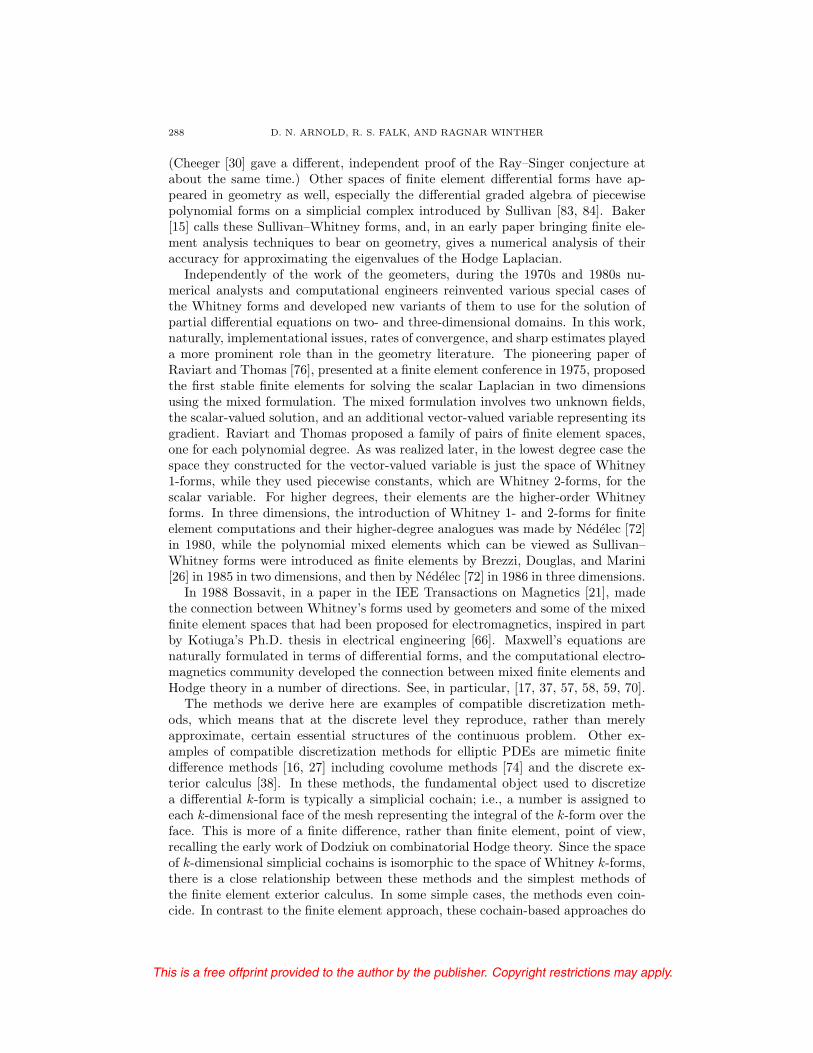
(Cheeger [30] gave a different, independent proof of the Ray–Singer conjecture atabout the same time.) Other spaces of finite element differential forms have ap-peared in geometry as well, especially the differential graded algebra of piecewisepolynomial forms on a simplicial complex introduced by Sullivan [83, 84]. Baker[15] calls these Sullivan–Whitney forms, and, in an early paper bringing finite ele-ment analysis techniques to bear on geometry, gives a numerical analysis of theiraccuracy for approximating the eigenvalues of the Hodge Laplacian.
Independently of the work of the geometers, during the 1970s and 1980s nu-merical analysts and computational engineers reinvented various special cases ofthe Whitney forms and developed new variants of them to use for the solution ofpartial differential equations on two- and three-dimensional domains. In this work,naturally, implementational issues, rates of convergence, and sharp estimates playeda more prominent role than in the geometry literature. The pioneering paper ofRaviart and Thomas [76], presented at a finite element conference in 1975, proposedthe first stable finite elements for solving the scalar Laplacian in two dimensionsusing the mixed formulation. The mixed formulation involves two unknown fields,the scalar-valued solution, and an additional vector-valued variable representing itsgradient. Raviart and Thomas proposed a family of pairs of finite element spaces,one for each polynomial degree. As was realized later, in the lowest degree case thespace they constructed for the vector-valued variable is just the space of Whitney1-forms, while they used piecewise constants, which are Whitney 2-forms, for thescalar variable. For higher degrees, their elements are the higher-order Whitneyforms. In three dimensions, the introduction of Whitney 1- and 2-forms for finiteelement computations and their higher-degree analogues was made by Nedelec [72]in 1980, while the polynomial mixed elements which can be viewed as Sullivan–Whitney forms were introduced as finite elements by Brezzi, Douglas, and Marini[26] in 1985 in two dimensions, and then by Nedelec [72] in 1986 in three dimensions.
In 1988 Bossavit, in a paper in the IEE Transactions on Magnetics [21], madethe connection between Whitney’s forms used by geometers and some of the mixedfinite element spaces that had been proposed for electromagnetics, inspired in partby Kotiuga’s Ph.D. thesis in electrical engineering [66]. Maxwell’s equations arenaturally formulated in terms of differential forms, and the computational electro-magnetics community developed the connection between mixed finite elements andHodge theory in a number of directions. See, in particular, [17, 37, 57, 58, 59, 70].
The methods we derive here are examples of compatible discretization meth-ods, which means that at the discrete level they reproduce, rather than merelyapproximate, certain essential structures of the continuous problem. Other ex-amples of compatible discretization methods for elliptic PDEs are mimetic finitedifference methods [16, 27] including covolume methods [74] and the discrete ex-terior calculus [38]. In these methods, the fundamental object used to discretizea differential k-form is typically a simplicial cochain; i.e., a number is assigned toeach k-dimensional face of the mesh representing the integral of the k-form over theface. This is more of a finite difference, rather than finite element, point of view,recalling the early work of Dodziuk on combinatorial Hodge theory. Since the spaceof k-dimensional simplicial cochains is isomorphic to the space of Whitney k-forms,there is a close relationship between these methods and the simplest methods ofthe finite element exterior calculus. In some simple cases, the methods even coin-cide. In contrast to the finite element approach, these cochain-based approaches do
This is a free offprint provided to the author by the publisher. Copyright restrictions may apply.
FINITE ELEMENT EXTERIOR CALCULUS 289
not naturally generalize to higher-order methods. Discretizations of exterior calcu-lus and Hodge theory have also been used for purposes other than solving partialdifferential equations. For example, discrete forms which are identical or closelyrelated to cochains or the corresponding Whitney forms play an important role ingeometric modeling, parameterization, and computer graphics. See for example[50, 54, 56, 87].
1.4. Highlights of the finite element exterior calculus. We close this in-troduction by highlighting some of the features that are unique or much moreprominent in the finite element exterior calculus than in earlier works.
• We work in an abstract Hilbert space setting that captures the fundamentalstructures of the Hodge theory of Riemannian manifolds, but applies moregenerally. In fact, the paper proceeds in two parts, first the abstract theoryfor Hilbert complexes, and then the application to the de Rham complexand Hodge theory and other applications.
• Mixed formulations based on saddle point variational principles play aprominent role. In particular, the algorithms we use to approximate theHodge Laplacian are based on a mixed formulation, as is the analysis of thealgorithms. This is in contrast to the approach in the geometry literature,where the underlying variational principle is a minimization principle. Inthe case of the simplest elements, the Whitney elements, the two meth-ods are equivalent. That is, the discrete solution obtained by the mixedfinite element method using Whitney forms, is the same as that obtainedby Dodziuk’s combinatorial Laplacian. However, the different viewpointleads naturally to different approaches to the analysis. The use of Whitneyforms for the mixed formulation is obviously a consistent discretization,and the key to the analysis is to establish stability (see the next sectionfor the terminology). However, for the minimization principle, it is unclearwhether Whitney forms provide a consistent approximation, because theydo not belong to the domain of the exterior coderivative, and, as remarkedin [40], this greatly complicates the analysis. The results we obtain areboth more easily proven and sharper.
• Our analysis is based on two main properties of the subspaces used to dis-cretize the Hilbert complex. First, they can be formed into subcomplexes,which is a key assumption in much of the work we have discussed. Second,there exist a bounded cochain projection from the Hilbert complex to thesubcomplex. This is a new feature. In previous work, a cochain projectionoften played a major role, but it was not bounded, and the existence ofbounded cochain projections was not realized. In fact, they exist quite gen-erally (see Theorem 3.7), and we review the construction for the de Rhamcomplex in Section 5.5.
• Since we are interested in actual numerical computations, it is importantthat our spaces be efficiently implementable. This is not true for all piece-wise polynomial spaces. As explained in the next section, finite elementspaces are a class of piecewise polynomial spaces that can be implementedefficiently by local computations thanks to the existence of degrees of free-dom, and the construction of degrees of freedom and local bases is animportant part of the finite element exterior calculus.

This is a free offprint provided to the author by the publisher. Copyright restrictions may apply.
290 D. N. ARNOLD, R. S. FALK, AND RAGNAR WINTHER
• For the same reason, high-order piecewise polynomials are of great im-portance, and all the constructions and analysis of finite element exteriorcalculus carries through for polynomials of arbitrary degree.
• A prominent aspect of the finite element exterior calculus is the role oftwo families of spaces of polynomial differential forms, PrΛ
k and P−r Λk,
where the index r ≥ 1 denotes the polynomial degree and k ≥ 0 the formdegree. These are the shape functions for corresponding finite elementspaces of differential k-forms which include, as special cases, the Lagrangefinite element family, and most of the stable finite element spaces thathave been used to define mixed formulations of the Poisson or Maxwell’sequations. The space P−
1 Λk is the classical space of Whitney k-forms. Thefinite element spaces based on PrΛ
k are the spaces of Sullivan–Whitneyforms. We show that for each polynomial degree r, there are 2n−1 ways toform these spaces in de Rham subcomplexes for a domain in n dimensions.The unified treatment of the spaces PrΛ
k and P−r Λk, particularly their
connections via the Koszul complex, is new to the finite element exteriorcalculus.
The finite element exterior calculus unifies many of the finite element methodsthat have been developed for solving PDEs arising in fluid and solid mechanics,electromagnetics, and other areas. Consequently, the methods developed here havebeen widely implemented and applied in scientific and commercial programs suchas GetDP [42], FEniCS [44], EMSolve [45], deal.II [46], Diffpack [61], Getfem++[77], and NGSolve [78]. We also note that, as part of a recent programming effortconnected with the FEniCS project, Logg and Mardal [69] have implemented thefull set of finite element spaces developed in this paper, strictly following the finiteelement exterior framework as laid out here and in [8].
2. Finite element discretizations
In this section we continue the introduction to the finite element method begunabove. We move beyond the case of one dimension and consider not only the for-mulation of the method, but also its analysis. To motivate the theory developedlater in this paper, we present further examples that illustrate how for some prob-lems, even rather simple ones, deriving accurate finite element methods is not astraightforward process.
2.1. Galerkin methods and finite elements. We consider first a simple prob-lem, which can be discretized in a straightforward way, namely the Dirichlet prob-lem for Poisson’s equation in a polyhedral domain Ω ⊂ Rn:
(4) −∆u = f in Ω, u = 0 on ∂Ω.
This is the generalization to n dimensions of the problem (1) discussed in theintroduction, and the solution may again be characterized as the minimizer of anenergy functional analogous to (2) or as the solution of a weak problem analogous to(3). This leads to discretization just as for the one-dimensional case, by choosing a
trial space Vh ⊂ H1(Ω) and defining the approximate solution uh ∈ Vh by Galerkin’smethod: ∫
Ω
graduh(x) · grad v(x) dx =
∫Ω
f(x)v(x) dx, v ∈ Vh.
This is a free offprint provided to the author by the publisher. Copyright restrictions may apply.
FINITE ELEMENT EXTERIOR CALCULUS 291
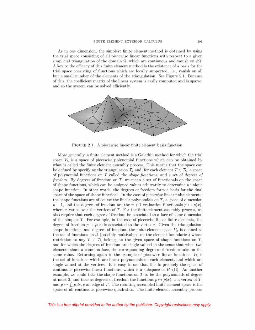
As in one dimension, the simplest finite element method is obtained by usingthe trial space consisting of all piecewise linear functions with respect to a givensimplicial triangulation of the domain Ω, which are continuous and vanish on ∂Ω.A key to the efficacy of this finite element method is the existence of a basis for thetrial space consisting of functions which are locally supported, i.e., vanish on allbut a small number of the elements of the triangulation. See Figure 2.1. Becauseof this, the coefficient matrix of the linear system is easily computed and is sparse,and so the system can be solved efficiently.
Figure 2.1. A piecewise linear finite element basis function.
More generally, a finite element method is a Galerkin method for which the trialspace Vh is a space of piecewise polynomial functions which can be obtained bywhat is called the finite element assembly process. This means that the space canbe defined by specifying the triangulation Th and, for each element T ∈ Th, a spaceof polynomial functions on T called the shape functions, and a set of degrees offreedom. By degrees of freedom on T , we mean a set of functionals on the spaceof shape functions, which can be assigned values arbitrarily to determine a uniqueshape function. In other words, the degrees of freedom form a basis for the dualspace of the space of shape functions. In the case of piecewise linear finite elements,the shape functions are of course the linear polynomials on T , a space of dimensionn + 1, and the degrees of freedom are the n + 1 evaluation functionals p → p(x),where x varies over the vertices of T . For the finite element assembly process, wealso require that each degree of freedom be associated to a face of some dimensionof the simplex T . For example, in the case of piecewise linear finite elements, thedegree of freedom p → p(x) is associated to the vertex x. Given the triangulation,shape functions, and degrees of freedom, the finite element space Vh is defined asthe set of functions on Ω (possibly multivalued on the element boundaries) whoserestriction to any T ∈ Th belongs to the given space of shape functions on T ,and for which the degrees of freedom are single-valued in the sense that when twoelements share a common face, the corresponding degrees of freedom take on thesame value. Returning again to the example of piecewise linear functions, Vh isthe set of functions which are linear polynomials on each element, and which aresingle-valued at the vertices. It is easy to see that this is precisely the space ofcontinuous piecewise linear functions, which is a subspace of H1(Ω). As anotherexample, we could take the shape functions on T to be the polynomials of degreeat most 2, and take as degrees of freedom the functions p → p(x), x a vertex of T ,and p →
∫ep ds, e an edge of T . The resulting assembled finite element space is the
space of all continuous piecewise quadratics. The finite element assembly process

This is a free offprint provided to the author by the publisher. Copyright restrictions may apply.
292 D. N. ARNOLD, R. S. FALK, AND RAGNAR WINTHER
insures the existence of a computable locally supported basis, which is importantfor efficient implementation.
2.2. Consistency, stability, and convergence. We now turn to the importantproblem of analyzing the error in the finite element method. To understand whena Galerkin method will produce a good approximation to the true solution, weintroduce the standard abstract framework. Let V be a Hilbert space, B : V ×V →R a bounded bilinear form, and F : V → R a bounded linear form. We assume theproblem to be solved can be stated in the form: Find u ∈ V such that
B(u, v) = F (v), v ∈ V.
This problem is called well-posed if for each F ∈ V ∗, there exists a unique solutionu ∈ V and the mapping F → u is bounded, or, equivalently, if the operator L :V → V ∗ given by 〈Lu, v〉 = B(u, v) is an isomorphism. For the Dirichlet problemfor Poisson’s equation,
(5) V = H1(Ω), B(u, v) =
∫Ω
gradu(x) · grad v(x) dx, F (v) =
∫Ω
f(x)v(x) dx.
A generalized Galerkin method for the abstract problem begins with a finite-dimensional normed space Vh (not necessarily a subspace of V ), a bilinear formBh : Vh × Vh → R, and a linear form Fh : Vh → R, and defines uh ∈ Vh by
(6) Bh(uh, v) = Fh(v), v ∈ Vh.
A Galerkin method is the special case of a generalized Galerkin method for which Vh
is a subspace of V and the forms Bh and Fh are simply the restrictions of the formsB and F to the subspace. The more general setting is important since it allowsthe incorporation of additional approximations, such as numerical integration toevaluate the integrals, and also allows for situations in which Vh is not a subspaceof V . Although we do not treat approximations such as numerical integration inthis paper, for the fundamental discretization method that we study, namely themixed method for the abstract Hodge Laplacian introduced in Section 3.4, the trialspace Vh is not a subspace of V , since it involves discrete harmonic forms whichwill not, in general, belong to the space of harmonic forms.
The generalized Galerkin method (6) may be written Lhuh = Fh where Lh :Vh → V ∗
h is given by 〈Lhu, v〉 = Bh(u, v), u, v ∈ Vh. If the finite-dimensionalproblem is nonsingular, then we define the norm of the discrete solution operator,‖L−1
h ‖L(V ∗h ,Vh), as the stability constant of the method.
Of course, in approximating the original problem determined by V , B, and F ,by the generalized Galerkin method given by Vh, Bh, and Fh, we intend that thespace Vh in some sense approximates V and that the discrete forms Bh and Fh
in some sense approximate B and F . This is the essence of consistency. Ourgoal is to prove that the discrete solution uh approximates u in an appropriatesense (convergence). In order to make these notions precise, we need to compare afunction in V to a function in Vh. To this end, we suppose that there is a restrictionoperator πh : V → Vh, so that πhu is thought to be close to u. Then the consistencyerror is simply Lhπhu−Fh and the error in the generalized Galerkin method whichwe wish to control is πhu − uh. We immediately get a relation between the errorand the consistency error:
πhu− uh = L−1h (Lhπhu− Fh),

This is a free offprint provided to the author by the publisher. Copyright restrictions may apply.
FINITE ELEMENT EXTERIOR CALCULUS 293
and so the norm of the error is bounded by the product of the stability constantand the norm of the consistency error:
‖πhu− uh‖Vh≤ ‖L−1
h ‖L(V ∗h ,Vh)‖Lhπhu− Fh‖V ∗
h.
Stated in terms of the bilinear form Bh, the norm of the consistency error can bewritten as
‖Lhπhu− Fh‖V ∗h= sup
0=v∈Vh
Bh(πhu, v)− Fh(v)
‖v‖Vh
.
As for stability, the finite-dimensional problem is nonsingular if and only if
γh := inf0=u∈Vh
sup0=v∈Vh
Bh(u, v)
‖u‖Vh‖v‖Vh
> 0,
and the stability constant is then given by γ−1h .
Often we consider a sequence of spaces Vh and forms Bh and Fh, where we thinkof h > 0 as an index accumulating at 0. The corresponding generalized Galerkinmethod is consistent if the Vh norm of the consistency error tends to zero with hand it is stable if the stability constant γ−1
h is uniformly bounded. For a consistent,stable generalized Galerkin method, ‖πhu − uh‖Vh
tends to zero; i.e., the methodis convergent.
In the special case of a Galerkin method, we can bound the consistency error
sup0=v∈Vh
Bh(πhu, v)− Fh(v)
‖v‖V= sup
0=v∈Vh
B(πhu− u, v)
‖v‖V≤ ‖B‖‖πhu− u‖V .
In this case it is natural to choose the restriction πh to be the orthogonal projectiononto Vh, and so the consistency error is bounded by the norm of the bilinear formtimes the error in the best approximation of the solution. Thus we obtain
‖πhu− uh‖V ≤ γ−1h ‖B‖ inf
v∈Vh
‖u− v‖V .
Combining this with the triangle inequality, we obtain the basic error estimate forGalerkin methods
(7) ‖u− uh‖V ≤ (1 + γ−1h ‖B‖) inf
v∈Vh
‖u− v‖V .
(In fact, in this Hilbert space setting, the quantity in parentheses can be replacedwith γ−1
h ‖B‖; see [89].) Note that a Galerkin method is consistent as long as thesequence of subspaces Vh is approximating in V in the sense that
(8) limh→0
infv∈Vh
‖u− v‖V = 0, u ∈ V.
A consistent, stable Galerkin method converges, and the approximation given bythe method is quasi-optimal; i.e., up to multiplication by a constant, it is as goodas the best approximation in the subspace.
In practice, it can be quite difficult to show that the finite-dimensional problemis nonsingular and to bound the stability constant, but there is one important casein which it is easy, namely when the form B is coercive, i.e., when there is a positiveconstant α for which
B(v, v) ≥ α‖v‖2V , v ∈ V,
and so γh ≥ α. The bilinear form (5) for Poisson’s equation is coercive, as followsfrom Poincare’s inequality. This explains, and can be used to prove, the goodconvergence behavior of the method depicted in Figure 1.1.

This is a free offprint provided to the author by the publisher. Copyright restrictions may apply.
294 D. N. ARNOLD, R. S. FALK, AND RAGNAR WINTHER
2.3. Computational examples.
2.3.1. Mixed formulation of the Laplacian. For an example of a problem that fitsin the standard abstract framework with a noncoercive bilinear form, we take themixed formulation of the Dirichlet problem for Poisson’s equation, already intro-duced in one dimension in Section 1.1. Just as there, we begin by writing Poisson’sequation as the first-order system
(9) σ = − gradu, div σ = f.
The pair (σ, u) can again be characterized variationally as the unique critical point(a saddle point) of the functional
I(σ, u) =
∫Ω
(1
2σ · σ − u div σ) dx+
∫Ω
fu dx
over H(div; Ω)× L2(Ω), where H(div; Ω) = σ ∈ L2(Ω) : div σ ∈ L2(Ω). Equiva-lently, it solves the weak problem: Find σ ∈ H(div; Ω), u ∈ L2(Ω) satisfying∫
Ω
σ · τ dx−∫Ω
u div τ dx = 0, τ ∈ H(div; Ω),∫Ω
div σv dx =
∫Ω
fv dx, v ∈ L2(Ω).
This mixed formulation of Poisson’s equation fits in the abstract framework ifwe define V = H(div; Ω)× L2(Ω),
B(σ, u; τ, v) =
∫Ω
σ · τ dx−∫Ω
u div τ dx+
∫Ω
div σv dx, F (τ, v) =
∫Ω
fv dx.
In this case the bilinear form B is not coercive, and so the choice of subspaces andthe analysis is not so simple as for the standard finite element method for Poisson’sequation, a point we already illustrated in the one-dimensional case.
Finite element discretizations based on such saddle point variational principlesare called mixed finite element methods. Thus a mixed finite element for Poisson’sequation is obtained by choosing subspaces Σh ⊂ H(div; Ω) and Vh ⊂ L2(Ω) andseeking a critical point of I over Σh × Vh. The resulting Galerkin method has theform: Find σh ∈ Σh, uh ∈ Vh satisfying∫
Ω
σh · τ dx−∫Ω
uh div τ dx = 0, τ ∈ Σh,
∫Ω
div σhv dx =
∫Ω
fv dx, v ∈ Vh.
This again reduces to a linear system of algebraic equations.Since the bilinear form is not coercive, it is not automatic that the linear system
is nonsingular, i.e., that for f = 0, the only solution is σh = 0, uh = 0. Choosingτ = σh and v = uh and adding the discretized variational equations, it followsimmediately that when f = 0, σh = 0. However, uh need not vanish unless thecondition that
∫Ωuh div τ dx = 0 for all τ ∈ Σh implies that uh = 0. In particular,
this requires that dim(div Σh) ≥ dimVh. Thus, even nonsingularity of the approxi-mate problem depends on a relationship between the two finite-dimensional spaces.Even if the linear system is nonsingular, there remains the issue of stability, i.e., ofa uniform bound on the inverse operator.
As mentioned earlier, the combination of continuous piecewise linear elements forσ and piecewise constants for u is not stable in two dimensions. The simplest stableelements use the piecewise constants for u, and the lowest-order Raviart-Thomaselements for σ. These are finite elements defined with respect to a triangular

This is a free offprint provided to the author by the publisher. Copyright restrictions may apply.
FINITE ELEMENT EXTERIOR CALCULUS 295
mesh by shape functions of the form (a + bx1, c + bx2) and one degree of freedomfor each edge e, namely σ →
∫eσ · n ds. We show in Figure 2.2 two numerical
computations that demonstrate the difference between an unstable and a stablechoice of elements for this problem. The stable method accurately approximatesthe true solution u = x(1− x)y(1− y) on (0, 1)× (0, 1) with a piecewise constant,while the unstable method is wildly oscillatory.
−0.15
0.05
0.25
0
0.0312
0.0625
Figure 2.2. Approximation of the mixed formulation for Pois-son’s equation using piecewise constants for u and for σ usingeither continuous piecewise linears (left), or Raviart–Thomas el-ements (right). The plotted quantity is u in each case.
This problem is a special case of the Hodge Laplacian with k = n as discussedbriefly in Section 4.2; see especially Section 4.2.4. The error analysis for a variety offinite element methods for this problem, including the Raviart–Thomas elements, isthus a special case of the general theory of this paper, yielding the error estimatesin Section 5.6.
2.3.2. The vector Laplacian on a nonconvex polygon. Given the subtlety of findingstable pairs of finite element spaces for the mixed variational formulation of Pois-son’s equation, we might choose to avoid this formulation, in favor of the standardformulation, which leads to a coercive bilinear form. However, while the standardformulation is easy to discretize for Poisson’s equation, additional issues arise al-ready if we try to discretize the vector Poisson equation. For a domain Ω in R3
with unit outward normal n, this is the problem
(10) − grad div u+ curl curlu = f, in Ω, u · n = 0, curlu× n = 0, on ∂Ω.
The solution of this problem can again be characterized as the minimizer of anappropriate energy functional,
(11) J(u) =1
2
∫Ω
(| div u|2 + | curlu|2) dx−∫Ω
f · u dx,
but this time over the space H(curl; Ω) ∩ H(div; Ω), where H(curl; Ω) = u ∈L2(Ω) | curlu ∈ L2(Ω) and H(div; Ω) = u ∈ H(div; Ω) |u · n = 0 on ∂Ω withH(div; Ω) defined above. This problem is associated to a coercive bilinear form,but a standard finite element method based on a trial subspace of the energy space

This is a free offprint provided to the author by the publisher. Copyright restrictions may apply.
296 D. N. ARNOLD, R. S. FALK, AND RAGNAR WINTHER
H(curl; Ω) ∩ H(div; Ω), e.g., using continuous piecewise linear vector functions,is very problematic. In fact, as we shall illustrate shortly, if the domain Ω is anonconvex polyhedron, for almost all f the Galerkin method solution will convergeto a function that is not the true solution of the problem! The essence of thisunfortunate situation is that any piecewise polynomial subspace of H(curl; Ω) ∩H(div; Ω) is a subspace of H1(Ω)∩H(div; Ω), and this space is a closed subspace of
H(curl; Ω)∩ H(div; Ω). For a nonconvex polyhedron, it is a proper closed subspaceand generally the true solution will not belong to it, due to a singularity at thereentrant corner. Thus the method, while stable, is inconsistent. For more on thisexample, see [35].
An accurate approximation of the vector Poisson equation can be obtained froma mixed finite element formulation, based on the system:
σ = − div u, gradσ + curl curlu = f in Ω, u · n = 0, curlu× n = 0 on ∂Ω.
Writing this system in weak form, we obtain the mixed formulation of the problem:find σ ∈ H1(Ω), u ∈ H(curl; Ω) satisfying∫
Ω
στ dx−∫Ω
u · grad τ dx = 0, τ ∈ H1(Ω),∫Ω
gradσ · v dx+
∫Ω
curlu · curl v dx =
∫Ω
f · v dx, v ∈ H(curl; Ω).
In contrast to a finite element method based on minimizing the energy (11), afinite element approximation based on the mixed formulation uses separate trialsubspaces ofH1(Ω) andH(curl; Ω), rather than a single subspace of the intersection
H(curl; Ω) ∩ H(div; Ω).We now illustrate the nonconvergence of a Galerkin method based on energy
minimization and the convergence of one based on the mixed formulation, via com-putations in two space dimensions (so now the curl of a vector u is the scalar∂u2/∂x1 − ∂u1/∂x2). For the trial subspaces we make the simplest choices: forthe former method we use continuous piecewise linear functions and for the mixedmethod we use continuous piecewise linear functions to approximate σ ∈ H1(Ω)and a variant of the lowest-order Raviart–Thomas elements, for which the shapefunctions are the infinitesimal rigid motions (a − bx2, c + bx1) and the degrees offreedom are the tangential moments u →
∫eu · s ds for e an edge. The discrete so-
lutions obtained by the two methods for the problem when f = (−1, 0) are shownin Figure 2.3. As we shall show later in this paper, the mixed formulation gives anapproximation that provably converges to the true solution, while, as can be seenfrom comparing the two plots, the first approximation scheme gives a completelydifferent (and therefore inaccurate) result.
This problem is again a special case of the Hodge Laplacian, now with k = 1.See Section 4.2.2. The error analysis thus falls within the theory of this paper,yielding estimates as in Section 5.6.
2.3.3. The vector Laplacian on an annulus. In the example just considered, thefailure of a standard Galerkin method based on energy minimization to solve thevector Poisson equation was related to the reentrant corner of the domain and theresulting singular behavior of the solution. A quite different failure mode for thismethod occurs if we take a domain which is smoothly bounded, but not simplyconnected, e.g., an annulus. In that case, as discussed below in Section 3.2, the

This is a free offprint provided to the author by the publisher. Copyright restrictions may apply.
FINITE ELEMENT EXTERIOR CALCULUS 297
Figure 2.3. Approximation of the vector Laplacian by the stan-dard finite element method (left) and a mixed finite elementmethod (right). The former method totally misses the singularbehavior of the solution near the reentrant corner.
boundary value problem (10) is not well-posed except for special values of the forc-ing function f . In order to obtain a well-posed problem, the differential equationshould be solved only modulo the space of harmonic vector fields (or harmonic 1-forms), which is a one-dimensional space for the annulus, and the solution shouldbe rendered unique by enforcing orthogonality to the harmonic vector fields. If wechoose the annulus with radii 1/2 and 1, and forcing function f = (0, x), the result-ing solution, which can be computed accurately with a mixed formulation fallingwithin the theory of this paper, is displayed on the right in Figure 2.4. However,the standard Galerkin method does not capture the nonuniqueness and computesthe discrete solution shown on the left of the same figure, which is dominated by anapproximation of the harmonic vector field, and so is nothing like the true solution.
Figure 2.4. Approximation of the vector Laplacian on an annu-lus. The true solution shown here on the right is an (accurate) ap-proximation by a mixed method. It is orthogonal to the harmonicfields and satisfies the differential equation only modulo harmonicfields. The standard Galerkin solution using continuous piecewiselinear vector fields, shown on the left, is totally different.

This is a free offprint provided to the author by the publisher. Copyright restrictions may apply.
298 D. N. ARNOLD, R. S. FALK, AND RAGNAR WINTHER
2.3.4. The Maxwell eigenvalue problem. Another situation where a standard finiteelement method gives unacceptable results, but a mixed method succeeds, arises inthe approximation of elliptic eigenvalue problems related to the vector Laplacian orMaxwell’s equation. This will be analyzed in detail later in this paper, and here weonly present a simple but striking computational example. Consider the eigenvalueproblem for the vector Laplacian discussed above, which we write in mixed formas: find nonzero (σ, u) ∈ H1(Ω)×H(curl; Ω) and λ ∈ R satisfying
(12)
∫Ω
σ · τ dx−∫Ω
grad τ · u dx = 0, τ ∈ H1(Ω),∫Ω
gradσ · v dx+
∫Ω
curlu · curl v dx = λ
∫Ω
u · v dx, v ∈ H(curl; Ω).
As explained in Section 3.6.1, this problem can be split into two subproblems. Inparticular, if 0 = u ∈ H(curl; Ω) and if λ ∈ R solves the eigenvalue problem
(13)
∫Ω
curlu · curl v dx = λ
∫Ω
u · v dx, v ∈ H(curl; Ω),
and λ is not equal to zero, then (σ, u), λ is an eigenpair for (12) with σ = 0.We now consider the solution of the eigenvalue problem (13), with two different
choices of trial subspaces in H(curl; Ω). Again, to make our point, it is enoughto consider a two-dimensional case, and we consider the solution of (13) with Ω asquare of side length π. For this domain, the positive eigenvalues can be computedby separation of variables. They are of the form m2 + n2 with m and n integers:1, 1, 2, 4, 4, 5, 5, 8, . . .. If we approximate (13) using the space of continuous piecewiselinear vector fields as the trial subspace ofH(curl; Ω), the approximation fails badly.This is shown for an unstructured mesh in Figure 2.5 and for a structured crisscrossmesh in Figure 2.6, where the nonzero discrete eigenvalues are plotted. Note thevery different mode of failure for the two mesh types. For more discussion of thespurious eigenvalues arising using continuous piecewise linear vector fields on acrisscross mesh, see [20]. By contrast, if we use the lowest-order Raviart–Thomasapproximation of H(curl; Ω), as shown on the right of Figure 2.5, we obtain aprovably good approximation for any mesh. This is a very simple case of thegeneral eigenvalue approximation theory presented in Section 3.6 below.
0
1
2
3
4
5
6
7
8
9
10
0
1
2
3
4
5
6
7
8
9
10
Figure 2.5. Approximation of the nonzero eigenvalues of (13) onan unstructured mesh of the square (left) using continuous piece-wise linear finite elements (middle) and Raviart–Thomas elements(right). For the former, the discrete spectrum looks nothing likethe true spectrum, while for the later it is very accurate.

This is a free offprint provided to the author by the publisher. Copyright restrictions may apply.
FINITE ELEMENT EXTERIOR CALCULUS 299
0
1
2
3
4
5
6
7
8
9
10
Figure 2.6. Approximation of the nonzero eigenvalues of (13)using continuous piecewise linear elements on the structured meshshown. The first seven discrete nonzero eigenvalues converge totrue eigenvalues, but the eighth converges to a spurious value.
3. Hilbert complexes and their approximation
In this section, we construct a Hilbert space framework for finite element exteriorcalculus. The most basic object in this framework is a Hilbert complex, which ex-tracts essential features of the L2 de Rham complex. Just as the Hodge Laplacianis naturally associated with the de Rham complex, there is a system of variationalproblems, which we call the abstract Hodge Laplacian, associated to any Hilbertcomplex. Using a mixed formulation we prove that these abstract Hodge Laplacianproblems are well-posed. We next consider the approximation of Hilbert complexesusing finite-dimensional subspaces. Our approach emphasizes two key properties,the subcomplex property and the existence of bounded cochain projections. Thesesame properties prove to be precisely what is needed both to show that the ap-proximate Hilbert complex accurately reproduces geometrical quantities associatedto the complex, like cohomology spaces, and also to obtain error estimates for theapproximation of the abstract Hodge Laplacian source and eigenvalue problems,which is our main goal in this section. In the following section of the paper we willderive finite element subspaces in the concrete case of the de Rham complex andverify the hypotheses needed to apply the results of this section.
Although the L2 de Rham complex is the canonical example of a Hilbert complex,there are many others. In this paper, in Section 6, we consider some variations ofthe de Rham complex that allow us to treat more general PDEs and boundaryvalue problems. In the final section we briefly discuss the equations of elasticity,for which a very different Hilbert complex, in which one of the differentials is asecond-order PDE, is needed. Another useful feature of Hilbert complexes is that asubcomplex of a Hilbert complex is again such, and so the properties we establishfor them apply not only at the continuous, but also at the discrete level.
3.1. Basic definitions. We begin by recalling some basic definitions of homolog-ical algebra and functional analysis and establishing some notation.
3.1.1. Cochain complexes. Consider a cochain complex (V, d) of vector spaces, i.e.,a sequence of vector spaces V k and linear maps dk, called the differentials:
· · · → V k−1 dk−1
−−−→ V k dk
−→ V k+1 → · · ·with dk dk−1 = 0. Equivalently, we may think of such a complex as the gradedvector space V =
⊕V k, equipped with a graded linear operator d : V → V of
This is a free offprint provided to the author by the publisher. Copyright restrictions may apply.
300 D. N. ARNOLD, R. S. FALK, AND RAGNAR WINTHER
degree +1 satisfying d d = 0. A chain complex differs from a cochain complexonly in that the indices decrease. All the complexes we consider are nonnegativeand finite, meaning that V k = 0 whenever k is negative or sufficiently large.
Given a cochain complex (V, d), the elements of the null space Zk = Zk(V, d) ofdk are called the k-cocycles and the elements of the range Bk = Bk(V, d) of dk−1
the k-coboundaries. The kth cohomology group is defined to be the quotient spaceZk/Bk.
Given two cochain complexes (V, d) and (V ′, d′), a set of linear maps fk : V k →V ′k satisfying d′kfk = fk+1dk (i.e., a graded linear map f : V → V ′ of degree0 satisfying d′f = fd) is called a cochain map. When f is a cochain map, fk
maps k-cocycles to k-cocycles and k-coboundaries to k-coboundaries, and henceinduces a map f on the cohomology spaces. This map is functorial; i.e., it respectscomposition.
Let (V, d) be a cochain complex and (Vh, d) a subcomplex. In other words, V kh is
a subspace of V k and dkV kh ⊂ V k+1
h . Then the inclusion ih : Vh → V is a cochainmap and so induces a map of cohomology. If there exists a cochain projection ofV onto Vh, i.e., a cochain map πh such that πk
h : V k → V kh leaves the subspace V k
h
invariant, then πh ih = idVh, so πh ih = idZk
h/Bkh(where Zk
h := Zk(Vh, d) and
similarly for Bkh). We conclude that in this case ih is injective and πh is surjective.
In particular, the dimension of the cohomology spaces of the subcomplex is at mostthat of the supercomplex.
3.1.2. Closed operators on Hilbert space. This material can be found in many places,e.g., [64, Chapter III, §5 and Chapter IV, §5.2] or [90, Chapter II, §6 and ChapterVII].
By an operator T from a Hilbert space X to a Hilbert space Y , we mean a linearoperator from a subspace V of X, called the domain of T , into Y . The operatorT is not necessarily bounded and the domain V is not necessarily closed. We saythat the operator T is closed if its graph (x, Tx) |x ∈ V is closed in X × Y . Weendow the domain V with the graph norm inner product,
〈v, w〉V = 〈v, w〉X + 〈Tv, Tw〉Y .It is easy to check that this makes V a Hilbert space (i.e., complete) if and only ifT is closed, and moreover, that T is a bounded operator from V to Y . Of course,the null space of T is the set of those elements of its domain that it maps to 0,and the range of T is T (V ). The null space of a closed operator from X to Y is aclosed subspace of X, but its range need not be closed in Y (even if the operatoris defined on all of X and is bounded).
The operator T is said to be densely defined if its domain V is dense in X. Inthis case the adjoint operator T ∗ from Y to X is defined to be the operator whosedomain consists of all y ∈ Y for which there exists x ∈ X with
〈x, v〉X = 〈y, Tv〉Y , v ∈ V,
in which case T ∗y = x (well-defined since V is dense). If T is closed and denselydefined, then T ∗ is as well and T ∗∗ = T . Moreover, the null space of T ∗ is theorthogonal complement of the range of T in Y . Finally, by the closed range theorem,the range of T is closed in Y if and only if the range of T ∗ is closed in X.
If the range of a closed linear operator is of finite codimension, i.e., dimY/T (V ) <∞, then the range is closed [60, Lemma 19.1.1].

This is a free offprint provided to the author by the publisher. Copyright restrictions may apply.
FINITE ELEMENT EXTERIOR CALCULUS 301
3.1.3. Hilbert complexes. A Hilbert complex is a sequence of Hilbert spaces W k andclosed, densely-defined linear operators dk from W k to W k+1 such that the rangeof dk is contained in the domain of dk+1 and dk+1 dk = 0. A Hilbert complexis bounded if, for each k, dk is a bounded linear operator from W k to W k+1. Inother words, a bounded Hilbert complex is a cochain complex in the category ofHilbert spaces. A Hilbert complex is closed if for each k, the range of dk is closedin W k+1. A Fredholm complex is a Hilbert complex for which the range of dk
is finite codimensional in the null space of dk+1 (and so is closed). Hilbert andFredholm complexes have been discussed by various authors working in geometryand topology. Bruning and Lesch [28] have advocated for them as an abstraction ofelliptic complexes on manifolds and applied them to spectral geometry on singularspaces. Glotko [53] used them to define a generalization of Sobolev spaces onRiemannian manifolds and to study their compactness properties, and Gromovand Shubin [55] used them to define topological invariants of manifolds.
Associated to any Hilbert complex (W,d) is a bounded Hilbert complex (V, d),called the domain complex, for which the space V k is the domain of dk, endowedwith the inner product associated to the graph norm:
〈u, v〉V k = 〈u, v〉Wk + 〈dku, dkv〉Wk+1 .
Then dk is a bounded linear operator from V k to V k+1, and so (V, d) is indeed abounded Hilbert complex. The domain complex is closed or Fredholm if and onlyif the original complex (W,d) is.
Of course, for a Hilbert complex (W,d), we have the null spaces and rangesZk and Bk. Utilizing the inner product, we define the space of harmonic formsHk = Zk ∩ Bk⊥, the orthogonal complement of Bk in Zk. It is isomorphic to
the reduced cohomology space Zk/Bk or, for a closed complex, to the cohomologyspace Zk/Bk. For a closed Hilbert complex, we immediately obtain the Hodgedecomposition
(14) W k = Bk ⊕ H
k ⊕ Zk⊥W .
For the domain complex (V, d), the null space, range, and harmonic forms are thesame spaces as for the original complex, and the Hodge decomposition is
V k = Bk ⊕ H
k ⊕ Zk⊥V ,
where the third summand Zk⊥V = Zk⊥W ∩ V k.Continuing to use the Hilbert space structure, we define the dual complex (W,d∗),
which is a Hilbert chain complex rather than a cochain complex. The dual complexuses the same spaces W i, with the differential d∗k being the adjoint of dk−1, so d∗k isa closed, densely-defined operator from W k to W k−1, whose domain we denote byV ∗k . The dual complex is closed or bounded if and only if the original complex is.
We denote by Z∗k = Bk⊥W the null space of d∗k, and by B∗
k the range of d∗k+1. Thus
Hk = Zk ∩ Z∗k is the space of harmonic forms both for the original complex and the
dual complex. Since Zk⊥W = B∗k, the Hodge decomposition (14) can be written as
(15) W k = Bk ⊕ H
k ⊕B∗k.
We henceforth simply write Zk⊥ for Zk⊥V .Let (W,d) be a closed Hilbert complex with domain complex (V, d). Then dk is
a bounded bijection from Zk⊥ to the Hilbert space Bk+1 and hence, by Banach’s
This is a free offprint provided to the author by the publisher. Copyright restrictions may apply.
302 D. N. ARNOLD, R. S. FALK, AND RAGNAR WINTHER
bounded inverse theorem, there exists a constant cP such that
(16) ‖v‖V ≤ cP ‖dkv‖W , v ∈ Zk⊥,
which we refer to as a Poincare inequality. We remark that the condition that Bk
is closed is not only sufficient to obtain (16), but also necessary.The subspace V k ∩ V ∗
k of W k is a Hilbert space with the norm
‖v‖2V ∩V ∗ = ‖v‖2V + ‖v‖2V ∗ = 2‖v‖2W + ‖dkv‖2W + ‖d∗kv‖2Wand is continuously included in W k. We say that the Hilbert complex (W,d) hasthe compactness property if V k ∩V ∗
k is dense in W k and the inclusion is a compactoperator. Restricted to the space Hk of harmonic forms, the V k ∩V ∗
k norm is equal
to the W k norm (times√2). Therefore the compactness property implies that the
inclusion of Hk into itself is compact, so Hk is finite-dimensional. In summary, forHilbert complexes, compactness property =⇒ Fredholm =⇒ closed.
3.2. The abstract Hodge Laplacian and the mixed formulation. Given aHilbert complex (W,d), the operator L = dd∗ + d∗d is an unbounded operatorW k → W k called, in the case of the de Rham complex, the Hodge Laplacian. Werefer to it as the abstract Hodge Laplacian in the general situation. Its domain is
DL = u ∈ V k ∩ V ∗k | du ∈ V ∗
k+1, d∗u ∈ V k−1 .
If u solves Lu = f , then
(17) 〈du, dv〉+ 〈d∗u, d∗v〉 = 〈f, v〉, v ∈ V k ∩ V ∗k .
Note that, in this equation, and henceforth, we use 〈 · , · 〉 and ‖ · ‖ without sub-scripts, meaning the inner product and norm in the appropriate W k space.
The harmonic functions measure the extent to which the Hodge Laplacian prob-lem (17) is well-posed. The solutions to the homogeneous problem (f = 0) areprecisely the functions in Hk. Moreover, a necessary condition for a solution toexist for nonzero f ∈ W k is that f ⊥ Hk.
For computational purposes, a formulation of the Hodge Laplacian based on (17)may be problematic, even when there are no harmonic forms, because it may not bepossible to construct an efficient finite element approximation for the space V k∩V ∗
k .We have already seen an example of this in the discussion of the approximation ofa boundary value problem for the vector Laplacian in Section 2.3.2. Instead weintroduce another formulation, which is a generalization of the mixed formulationdiscussed in Section 2 and which, simultaneously, accounts for the nonuniquenessassociated with harmonic forms. With (W,d) a Hilbert complex, (V, d) the asso-ciated domain complex, and f ∈ W k given, we define the mixed formulation ofthe abstract Hodge Laplacian as the problem of finding (σ, u, p) ∈ V k−1 × V k ×Hk
satisfying
(18)
〈σ, τ 〉 − 〈dτ, u〉 = 0, τ ∈ V k−1,
〈dσ, v〉+ 〈du, dv〉+ 〈v, p〉 = 〈f, v〉, v ∈ V k,
〈u, q〉 = 0, q ∈ Hk.
Remark. The equations (18) are the Euler–Lagrange equations associated to a
variational problem. Namely, if we define the quadratic functional I : V k−1×V k ×Hk → R by
I(τ, v, q) =1
2〈τ, τ 〉 − 〈dτ, v〉 − 1
2〈dv, dv〉 − 〈v, q〉+ 〈f, v〉,

This is a free offprint provided to the author by the publisher. Copyright restrictions may apply.
FINITE ELEMENT EXTERIOR CALCULUS 303
then a point (σ, u, p) ∈ V k−1 × V k × Hk is a critical point of I if and only if (18)holds, and in this case,
I(σ, v, q) ≤ I(σ, u, p) ≤ I(τ, u, p), (τ, v, q) ∈ V k−1 × V k × Hk.
Thus the critical point is a saddle point.An important result is that if the Hilbert complex is closed, then the mixed
formulation is well-posed. The requirement that the complex is closed is crucial,since we rely on the Poincare inequality.
Theorem 3.1. Let (W,d) be a closed Hilbert complex with domain complex (V, d).The mixed formulation of the abstract Hodge Laplacian is well-posed. That is, forany f ∈ W k, there exists a unique (σ, u, p) ∈ V k−1 × V k × Hk satisfying (18).Moreover,
‖σ‖V + ‖u‖V + ‖p‖ ≤ c‖f‖,where c is a constant depending only on the Poincare constant cP in (16).
We shall prove Theorem 3.1 in Section 3.2.2. First, we interpret the mixedformulation.
3.2.1. Interpretation of the mixed formulation. The first equation states that ubelongs to the domain of d∗ and d∗u = σ ∈ V k−1. The second equation similarlystates that du belongs to the domain of d∗ and d∗du = f − p− dσ. Thus u belongsto the domain DL of L and solves the abstract Hodge Laplacian equation
Lu = f − p.
The harmonic form p is simply the orthogonal projection PHf of f onto Hk, requiredfor existence of a solution. Finally the third equation fixes a particular solution,through the condition u ⊥ Hk. Thus Theorem 3.1 establishes that for any f ∈ W k
there is a unique u ∈ DL such that Lu = f −PHf and u ⊥ Hk. We define Kf = u,so the solution operator K : W k → W k is a bounded linear operator mapping intoDL. The solution to the mixed formulation is
σ = d∗Kf, u = Kf, p = PHf.
The mixed formulation (18) is also intimately connected to the Hodge decompo-sition (15). Since dσ ∈ Bk, p ∈ Hk, and d∗du ∈ B∗
k, the expression f = dσ+p+d∗duis precisely the Hodge decomposition of f . In other words
PB = dd∗K, PB∗ = d∗dK,
where PB and PB∗ are the W k-orthogonal projections onto Bk and B∗k, respec-
tively. We also note that K commutes with d and d∗ in the sense that
dKf = Kdf, f ∈ V k, d∗Kg = Kd∗g, g ∈ V ∗k .
Indeed, if f ∈ V k and u = Kf , then u ∈ DL, which implies that du ∈ V k+1∩V ∗k+1.
Also d∗u ∈ V k−1, so d∗du = f − PHf − dd∗u ∈ V k. This shows that du ∈ DL.Clearly
Ldu = (dd∗ + d∗d)du = dd∗du = d(dd∗ + d∗d)u = dLu = df,
and both du and df are orthogonal to harmonic forms. This establishes that du =Kdf , i.e., dKf = Kdf . The second equation is established similarly.
If we restrict the data f in the abstract Hodge Laplacian to an element of B∗k
or of Bk, we get two other problems which are also of great use in applications.
This is a free offprint provided to the author by the publisher. Copyright restrictions may apply.
304 D. N. ARNOLD, R. S. FALK, AND RAGNAR WINTHER
The B∗ problem. If f ∈ B∗k, then u = Kf ∈ B∗
k satisfies
d∗du = f, u ⊥ Zk,
while σ = d∗u = 0, p = PHf = 0. The solution u can be characterized as theunique element of Zk⊥ such that
(19) 〈du, dv〉 = 〈f, v〉, v ∈ Zk⊥,
and any solution to this problem is a solution of Lu = f , and so is uniquelydetermined.The B problem. If f ∈ Bk, then u = Kf ∈ Bk satisfies dd∗u = f , while p = PHf =0. With σ = d∗u, the pair (σ, u) ∈ V k−1 ×Bk is the unique solution of
(20) 〈σ, τ 〉 − 〈dτ, u〉 = 0, τ ∈ V k−1, 〈dσ, v〉 = 〈f, v〉, v ∈ Bk,
and any solution to this problem is a solution of Lu = f , σ = d∗u, and so is uniquelydetermined.
3.2.2. Well-posedness of the mixed formulation. We now turn to the proof of The-orem 3.1. Let B : X ×X → R be a symmetric bounded bilinear form on a Hilbertspace X which satisfies the inf-sup condition
γ := inf0=y∈X
sup0=x∈X
B(x, y)
‖x‖X‖y‖X> 0.
Then the problem of finding x ∈ X such that B(x, y) = F (y) for all y ∈ X iswell-posed: it has a unique solution x for each F ∈ X∗, and ‖x‖X ≤ γ−1‖F‖X∗
[13]. The abstract Hodge Laplacian problem (18) is of this form, where B : [V k−1×V k × Hk]× [V k−1 × V k × Hk] → R denotes the bounded bilinear form
B(σ, u, p; τ, v, q) = 〈σ, τ 〉 − 〈dτ, u〉+ 〈dσ, v〉+ 〈du, dv〉+ 〈v, p〉 − 〈u, q〉,and F (τ, v, p) = 〈f, v〉.
The following theorem establishes the inf-sup condition and so implies Theo-rem 3.1.
Theorem 3.2. Let (W,d) be a closed Hilbert complex with domain complex (V, d).There exists a constant γ > 0, depending only on the constant cP in the Poincareinequality (16), such that for any (σ, u, p) ∈ V k−1×V k×Hk, there exists (τ, v, q) ∈V k−1 × V k × Hk with
B(σ, u, p; τ, v, q) ≥ γ(‖σ‖V + ‖u‖V + ‖p‖)(‖τ‖V + ‖v‖V + ‖q‖).
Proof. By the Hodge decomposition, u = uB + uH + u⊥, where uB = PBu, uH =PHu, and u⊥ = PB∗u. Since uB ∈ Bk, uB = dρ, for some ρ ∈ Zk−1⊥. Sincedu⊥ = du, we get using (16) that
(21) ‖ρ‖V ≤ cP ‖uB‖, ‖u⊥‖V ≤ cP ‖du‖,where cP ≥ 1 is the constant in Poincare’s inequality. Let
(22) τ = σ − 1
c2Pρ ∈ V k−1, v = u+ dσ + p ∈ V k, q = p− uH ∈ H
k.
From (21) and the orthogonality of the Hodge decomposition, we have
(23) ‖τ‖V + ‖v‖V + ‖q‖ ≤ C(‖σ‖V + ‖u‖V + ‖p‖).

This is a free offprint provided to the author by the publisher. Copyright restrictions may apply.
FINITE ELEMENT EXTERIOR CALCULUS 305
We also get, from a simple computation using (21) and (22), that
B(σ, u, p; τ, v, q)
= ‖σ‖2 + ‖dσ‖2 + ‖du‖2 + ‖p‖2 + ‖uH‖2 +1
c2P‖uB‖2 − 1
c2P〈σ, ρ〉
≥ 1
2‖σ‖2 + ‖dσ‖2 + ‖du‖2 + ‖p‖2 + ‖uH‖2 +
1
c2P‖uB‖2 − 1
2c4P‖ρ‖2
≥ 1
2‖σ‖2 + ‖dσ‖2 + ‖du‖2 + ‖p‖2 + ‖uH‖2 +
1
2c2P‖uB‖2
≥ 1
2‖σ‖2 + ‖dσ‖2 + 1
2‖du‖2 + ‖p‖2 + ‖uH‖2 +
1
2c2P‖uB‖2 + 1
2c2P‖u⊥‖2
≥ 1
2c2P(‖σ‖2V + ‖u‖2V + ‖p‖2).
The theorem easily follows from this bound and (23).
We close this section with two remarks. First we note that in fact Theorem 3.2establishes more than the well-posedness of the problem (18) stated in Theorem 3.1.It establishes that, for any G ∈ (V k−1)∗, F ∈ (V k)∗, and R ∈ (Hk)∗ (these arethe dual spaces furnished with the dual norms), there exists a unique (σ, u, p) ∈V k−1 × V k × Hk satisfying
〈σ, τ 〉 − 〈dτ, u〉 = G(τ ), τ ∈ V k−1,
〈dσ, v〉+ 〈du, dv〉+ 〈v, p〉 = F (v), v ∈ V k,
〈u, q〉 = R(q), q ∈ Hk,
and moreover the correspondence (σ, u, p) ↔ (F,G,R) is an isomorphism of V k−1×V k × Hk onto its dual space.
Second, we note that the above result bears some relation to a fundamentalresult in the theory of mixed finite element methods, due to Brezzi [24], which westate here.
Theorem 3.3. Let X and Y be Hilbert spaces and a : X ×X → R, b : X ×Y → R
bounded bilinear forms. Let Z = x ∈ X | b(x, y) = 0 ∀y ∈ Y , and suppose thatthere exist positive constants α and γ such that
(1) (coercivity in the kernel) a(z, z) ≥ α‖z‖2X , z ∈ Z,
(2) (inf-sup condition) inf0=y∈Y
sup0=x∈X
b(x, y)
‖x‖X‖y‖Y≥ γ.
Then, for all G ∈ X∗, F ∈ Y ∗, there exists a unique u ∈ X, v ∈ Y such that
(24)a(u, x) + b(x, v) = G(x), x ∈ X,
b(u, y) = F (y), y ∈ Y.
Moreover, ‖u‖X + ‖v‖Y ≤ c(‖G‖X∗ + ‖F‖Y ∗) with the constant c depending onlyon α, γ, and the norms of the bilinear forms a and b.
If we make the additional assumption (usually satisfied in applications of thistheorem) that the bilinear form a is symmetric and satisfies a(x, x) > 0 for all0 = x ∈ X, then this theorem can be viewed as a special case of Theorem 3.2.In fact, we define W 0 as the completion of X in the inner product given by a, let
This is a free offprint provided to the author by the publisher. Copyright restrictions may apply.
306 D. N. ARNOLD, R. S. FALK, AND RAGNAR WINTHER
W 1 = Y , and define d as the closed linear operator from W 0 to W 1 with domainX given by
〈dx, y〉Y = b(x, y), x ∈ X, y ∈ Y.
In this way we obtain a Hilbert complex (with just two spaces W 0 and W 1). Theinf-sup condition of Theorem 3.3 implies that d has closed range, so it is a closedHilbert complex, and so Poincare’s inequality holds. The associated abstract HodgeLaplacian is just the system (24), and from Theorem 3.2 and the first remark above,we have √
a(u, u) + ‖du‖Y + ‖v‖Y ≤ c(‖G‖X∗ + ‖F‖Y ∗).
But, using the coercivity in the kernel, the decomposition X = Z + Z⊥, andPoincare’s inequality, we get ‖u‖X ≤ C[
√a(u, u)+‖du‖Y ], which gives the estimate
from Brezzi’s theorem. Finally, we mention that we could dispense with the extraassumption about the symmetry and positivity of the bilinear form a, but thiswould require a slight generalization of Theorem 3.2, which we do not considerhere.
3.3. Approximation of Hilbert complexes. The remainder of this section willbe devoted to the approximation of quantities associated to a Hilbert complex, suchas the cohomology spaces, harmonic forms, and solutions to the Hodge Laplacian,by quantities associated to a subcomplex.
Let (W,d) be a Hilbert complex with domain complex (V, d), and suppose wechoose a finite-dimensional subspace V k
h of V k for each k. We assume that dV kh ⊂
V k+1h so that (Vh, d) is a subcomplex of (V, d). We also take W k
h to be the same
subspace V kh but endowed with the norm of W k. In this way we obtain a closed
(even bounded) Hilbert complex (Wh, d) with domain complex (Vh, d), and all theresults of Sections 3.1.3 and 3.2 apply to this subcomplex. Although the differentialfor the subcomplex is just the restriction of d, and so does not need a new notation,its adjoint d∗h : V k+1
h → V kh , defined by
〈d∗hu, v〉 = 〈u, dv〉, u ∈ V k+1h , v ∈ V k
h ,
is not the restriction of d∗. We use the notation Bh, Zh, B∗h = Z⊥
h , Hh, Kh, with theobvious meanings. We use the term discrete when we wish to emphasize quantitiesassociated to the subcomplex. For example, we refer to Hk
h as the space of discreteharmonic k-forms, and the discrete Hodge decomposition is
V kh = B
kh ⊕ H
kh ⊕ Z
k⊥h .
The W k-projections PBh: W k → Bk
h, PB∗h: W k → Zk⊥
h satisfy PBh= dd∗hKh
and PB∗h= d∗hdKh, respectively, when restricted to V k
h . We also have that Kh
commutes with both d and d∗h. Note that Bkh ⊂ Bk and Zk
h ⊂ Zk, but in generalHk
h is not contained in Hk, nor is Zk⊥h contained in Zk⊥.
In order that the subspaces V kh can be used effectively to approximate quantities
associated to the original complex, we require not only that they form a subcomplex,but of course we need to know something about the approximation of V k by V k
h ,i.e., an assumption that infv∈V k
h‖u−v‖V is sufficiently small for some or all u ∈ V k.
A third assumption, which plays an essential role in our analysis, is that there existsa bounded cochain projection πh from the complex (V, d) to the subcomplex (Vh, d).Explicitly, for each k, πk
h maps V k to V kh , leaves the subspace invariant, satisfies
dkπkh = πk+1
h dk, and there exists a constant c such that ‖πkhv‖V ≤ c‖v‖V for all
This is a free offprint provided to the author by the publisher. Copyright restrictions may apply.
FINITE ELEMENT EXTERIOR CALCULUS 307
v ∈ V k. In other words, we have the following commuting diagram relating thecomplex (V, d) to the subcomplex (Vh, d):
0 →V 0 d−−−−→ V 1 d−−−−→ · · · d−−−−→ V n → 0πh
πh
πh
0 →V 0h
d−−−−→ V 1h
d−−−−→ · · · d−−−−→ V nh → 0.
Note that a bounded projection gives quasi-optimal approximation:
‖u− πhu‖V = infv∈V k
h
‖(I − πh)(u− v)‖V ≤ c infv∈V k
h
‖u− v‖V .
We now present two results indicating that, under these assumptions, the spaceHk
h of discrete harmonic forms provides a faithful approximation of Hk. In the firstresult we show that a bounded cochain projection into a subcomplex of a boundedclosed Hilbert complex which satisfies a rather weak approximability assumption(namely (25) below), induces, not only a surjection, but an isomorphism on coho-mology.
Theorem 3.4. Let (V, d) be a bounded closed Hilbert complex, (Vh, d) a Hilbertsubcomplex, and πh a bounded cochain projection. Suppose that for all k,
(25) ‖q − πkhq‖V < ‖q‖V , 0 = q ∈ H
k.
Then the induced map on cohomology is an isomorphism.
Proof. We already know that the induced map is a surjection, so it is sufficient toprove that it is an injection. Thus, given z ∈ Zk with πhz ∈ Bk
h, we must provethat z ∈ Bk. By the Hodge decomposition, z = q + b with q ∈ Hk and b ∈ Bk. Wehave that πhz ∈ Bk
h by assumption and πhb ∈ Bkh since b ∈ Bk and πh is a cochain
map. Thus πhq = πhz − πhb ∈ Bkh ⊂ Bk, and so πhq ⊥ q. In view of (25), this
implies that q = 0, and so z ∈ Bk, as desired.
Remark. In applications, the space of harmonic forms, Hk, is a finite-dimensionalspace of smooth functions, and πh is a projection operator associated to a triangu-lation with mesh size h. The estimate (25) will then be satisfied for h sufficientlysmall. However, in the most important application, in which (V, d) is the de Rhamcomplex and (Vh, d) is a finite element discretization, πh induces an isomorphism oncohomology not only for h sufficiently small, but in fact for all h. See Section 5.6.
The second result relating Hk and Hkh is quantitative in nature, bounding the dis-
tance, or gap, between these two spaces. Recall that the gap between two subspacesE and F of a Hilbert space V is defined [64, Chapter IV, §2.1] by
(26) gap(E,F ) = max
(supu∈E‖u‖=1
infv∈F
‖u− v‖V , supv∈F‖v‖=1
infu∈E
‖u− v‖V).
Theorem 3.5. Let (V, d) be a bounded closed Hilbert complex, (Vh, d) a Hilbertsubcomplex, and πh a bounded cochain projection. Then
‖(I − PHh)q‖V ≤ ‖(I − πk
h)q‖V , q ∈ Hk,(27)
‖(I − PH)q‖V ≤ ‖(I − πkh)PHq‖V , q ∈ H
kh,(28)

This is a free offprint provided to the author by the publisher. Copyright restrictions may apply.
308 D. N. ARNOLD, R. S. FALK, AND RAGNAR WINTHER
gap(H
k,Hkh
)≤ sup
q∈Hk
‖q‖=1
‖(I − πkh)q‖V .(29)
Proof. Given q ∈ Hk, PHhq = PZh
q, since Zkh = Hk
h ⊕Bkh and q ⊥ Bk ⊃ Bk
h. Alsoπkhq ∈ Zk
h, since πh is a cochain map. This implies (27).If q ∈ Hk
h ⊂ Zkh ⊂ Zk, the Hodge decomposition gives us q − PHq ∈ Bk, so
πkh(q − PHq) ∈ Bk
h, and so is orthogonal to both the discrete harmonic form q andthe harmonic form PHq. Therefore
‖q − PHq‖V ≤ ‖q − PHq − πh(q − PHq)‖V = ‖(I − πkh)PHq‖V .
Finally (29) is an immediate consequence of (27) and (28).
Next we deduce another important property of a Hilbert subcomplex with abounded cochain projection. Since the complex (V, d) is closed and bounded, thePoincare inequality (16) holds (with the W and V norms coinciding). Now weobtain the Poincare inequality for the subcomplex with a constant that dependsonly on the Poincare constant for the supercomplex and the norm of the cochainprojection. In the applications, we will have a sequence of such subcomplexesrelated to a decreasing mesh size parameter, and this theorem will imply that thediscrete Poincare inequality is uniform with respect to the mesh parameter, anessential step in proving stability for numerical methods.
Theorem 3.6. Let (V, d) be a bounded closed Hilbert complex, (Vh, d) a Hilbertsubcomplex, and πk
h a bounded cochain projection. Then
‖v‖V ≤ cP ‖πkh‖‖dv‖V , v ∈ Z
k⊥h ,
where cP is the constant appearing in the Poincare inequality (16) and ‖πkh‖ denotes
the V k operator norm of πkh.
Proof. Given v ∈ Zk⊥h , define z ∈ Zk⊥ ⊂ V k by dz = dv. By (16), ‖z‖ ≤ cP ‖dv‖, so
it is enough to show that ‖v‖V ≤ ‖πh‖‖z‖V . Now, v−πhz ∈ V kh and d(v−πhz) = 0,
so v − πhz ∈ Zkh. Therefore
‖v‖2V = 〈v, πhz〉V + 〈v, v − πhz〉V = 〈v, πhz〉V ≤ ‖v‖V ‖πhz‖V ,and the result follows.
We have established several important properties possessed by a subcomplex of abounded closed Hilbert complex with bounded cochain projection. We also remarkthat from (28) and the triangle inequality, we have
(30) ‖q‖V ≤ c‖PHq‖V , q ∈ Hkh.
We close this section by presenting a converse result. Namely we show that ifthe discrete Poincare inequality and the bound (30) hold, then a bounded cochainprojection exists.
Theorem 3.7. Let (V, d) be a bounded closed Hilbert complex and (Vh, d) a sub-complex. Assume that
‖v‖V ≤ c1‖dv‖V , v ∈ Zk⊥h , and ‖q‖V ≤ c2‖PHq‖V , q ∈ H
kh,
for some constants c1 and c2. Then there exists a bounded cochain projection πh
from (V, d) to (Vh, d), and the V operator norm ‖πh‖ can be bounded in terms ofc1 and c2.

This is a free offprint provided to the author by the publisher. Copyright restrictions may apply.
FINITE ELEMENT EXTERIOR CALCULUS 309
Proof. As a first step of the proof we define an operator Qh : V k → Zk⊥h by
dQhv = PBhdv. By the first assumption, this operator is V -bounded since
‖Qhv‖V ≤ c1‖PBhdv‖ ≤ c1‖v‖V ,
and if v ∈ Vh, thenQhv = PB∗hv. By the second assumption, the operator PH|Hh
has
a bounded inverse Rh mapping Hk to Hkh. Note that for any v ∈ Zk
h, RhPHv = PHhv.
We now define πh : V k → V kh by
πh = PBh+RhPH(I −Qh) +Qh.
This operator is bounded in V k and invariant on V kh , since the three terms cor-
respond exactly to the discrete Hodge decomposition in this case. Furthermore,πhdv = PBh
dv = dQhv = dπhv, so πh is indeed a bounded cochain projection.
3.4. Stability and convergence of the mixed method. Next we consider aclosed Hilbert complex (W,d) and the Galerkin discretization of its Hodge Lapla-cian using finite-dimensional subspaces V k
h of the domain spaces V k. Our main
assumptions are those of Section 3.3: first, that dV kh ⊂ V k+1
h , so that we obtain asubcomplex
0 → V 0h
d−→ V 1h
d−→ · · · d−→ V nh → 0,
and, second, that there exists a bounded cochain projection πh from (V, d) to (Vh, d).Let f ∈ W k. In view of the mixed formulation (18), we take as an approximation
scheme: find σh ∈ V k−1h , uh ∈ V k
h , ph ∈ Hkh, such that
(31)
〈σh, τ 〉 − 〈dτ, uh〉 = 0, τ ∈ V k−1h ,
〈dσh, v〉+ 〈duh, dv〉+ 〈v, ph〉 = 〈f, v〉, v ∈ V kh ,
〈uh, q〉 = 0, q ∈ Hkh.
(Recall that we use 〈 · , · 〉 and ‖ · ‖ without subscripts for the W inner productand norm.) The discretization (31) is a generalized Galerkin method as discussedin Section 2.2. In the case that there are no harmonic forms (and therefore nodiscrete harmonic forms), it is a Galerkin method, but in general not, since Hk
h isnot in general a subspace of Hk. We may write the solution of (31), which alwaysexists and is unique in view of the results of Section 3.2.2, as
uh = KhPhf, σh = d∗huh, ph = PHhf,
where Ph : W k → V kh is the W k-orthogonal projection.
As in Section 2.2, we will bound the error in terms of the stability of the dis-cretization and the consistency error. We start by establishing a lower bound onthe inf-sup constant, i.e., an upper bound on the stability constant.
Theorem 3.8. Let (Vh, d) be a family of subcomplexes of the domain complex (V, d)of a closed Hilbert complex, parametrized by h and admitting uniformly V -boundedcochain projections. Then there exists a constant γh > 0, depending only on cP andthe norm of the projection operators πh, such that for any (σ, u, p) ∈ V k−1
h ×V kh ×Hk
h,
there exists (τ, v, q) ∈ V k−1h × V k
h × Hkh with
B(σ, u, p; τ, v, q) ≥ γh(‖σ‖V + ‖u‖V + ‖p‖)(‖τ‖V + ‖v‖V + ‖q‖).
Proof. This is just Theorem 3.2 applied to the Hilbert complex (Vh, d), combinedwith the fact that the constant in the Poincare inequality for V k
h is cP ‖πh‖ byTheorem 3.6.
This is a free offprint provided to the author by the publisher. Copyright restrictions may apply.
310 D. N. ARNOLD, R. S. FALK, AND RAGNAR WINTHER
From this stability result, we obtain the following error estimate.
Theorem 3.9. Let (Vh, d) be a family of subcomplexes of the domain complex (V, d)of a closed Hilbert complex, parametrized by h and admitting uniformly V -boundedcochain projections, and let (σ, u, p) ∈ V k−1 × V k × Hk be the solution of problem
(18) and (σh, uh, ph) ∈ V k−1h × V k
h × Hkh the solution of problem (31). Then
‖σ − σh‖V + ‖u− uh‖V + ‖p− ph‖≤ C( inf
τ∈V k−1h
‖σ − τ‖V + infv∈V k
h
‖u− v‖V + infq∈V k
h
‖p− q‖V + µ infv∈V k
h
‖PBu− v‖V ),
where µ = µkh = sup
r∈Hk
‖r‖=1
‖(I − πkh)r‖.
Proof. First observe that (σ, u, p) satisfies
B(σ, u, p; τh, vh, qh) = 〈f, vh〉 − 〈u, qh〉, (τh, vh, qh) ∈ V k−1h × V k
h × Hkh.
Let τ , v, and q be the V -orthogonal projections of σ, u, and p into V k−1h , V k
h , and
Hkh, respectively. Then, for any (τh, vh, qh) ∈ V k−1
h × V kh × Hk
h, we have
B(σh − τ, uh − v, ph − q; τh, vh, qh)
= B(σ − τ, u− v, p− q; τh, vh, qh) + 〈u, qh〉= B(σ − τ, u− v, p− q; τh, vh, qh) + 〈PHh
u, qh〉≤ C(‖σ − τ‖V + ‖u− v‖V + ‖p− q‖+ ‖PHh
u‖)(‖τh‖V + ‖vh‖V + ‖qh‖).
Theorem 3.8 then gives
(32) ‖σh − τ‖V + ‖uh − v‖V + ‖ph − q‖≤ C(‖σ − τ‖V + ‖u− v‖V + ‖p− q‖+ ‖PHh
u‖).
Using (27) and the boundedness of the projection πh we have
(33) ‖p− q‖ ≤ ‖(I − πh)p‖ ≤ C infq∈V k
h
‖p− q‖V .
Next we show that
‖PHhu‖ ≤ µ‖(I − πh)uB‖V .
Now u ⊥ Hk, so u = uB + u⊥, with uB ∈ Bk and u⊥ ∈ Zk⊥. Since Hkh ⊂ Zk,
PHhu⊥ = 0, and since πhuB ∈ Bk
h, PHhπhuB = 0. Let q = PHh
u/‖PHhu‖ ∈ Hk
h.By Theorem 3.5, there exists r ∈ Hk (and so r ⊥ Bk) with ‖r‖ ≤ 1 and
‖q − r‖ ≤ ‖(I − πh)r‖ ≤ supr∈H
k
‖r‖=1
‖(I − πh)r‖.
Therefore
(34) ‖PHhu‖ = 〈uB − πhuB, q − r〉
≤ ‖(I − πh)uB‖ supr∈H
k
‖r‖=1
‖(I − πh)r‖ ≤ c µ infv∈V k
h
‖PBu− v‖V ),
since πh is a bounded projection. The theorem follows from (32)–(34) and thetriangle inequality.

This is a free offprint provided to the author by the publisher. Copyright restrictions may apply.
FINITE ELEMENT EXTERIOR CALCULUS 311
To implement the discrete problem, we need to be able to compute the discreteharmonic forms. The following lemma shows one way to do this; namely, it showsthat the discrete harmonic forms can be computed as the elements of the null spaceof a matrix. For finite element approximations of the de Rham sequence, whichis the most canonical example of this theory and which will be discussed below, itis often possible to compute the discrete harmonic forms more directly. See, forexample, [2].
Lemma 3.10. Consider the homogeneous linear system: find (σh, uh) ∈ V k−1h ×V k
h
such that
〈σh, τ 〉 = 〈dτ, uh〉, τ ∈ V k−1h ,
〈dσh, v〉+ 〈duh, dv〉 = 0, v ∈ V kh .
Then (σh, uh) is a solution if and only if σh = 0 and uh ∈ Hkh.
Proof. Clearly (0, uh) is a solution if uh ∈ Hkh. On the other hand, if (σh, uh) is a
solution, by taking τ = σh, v = uh, and combining the two equations, we find that‖σh‖2 + ‖duh‖2 = 0, so that σh = 0 and duh = 0. Then the first equation implies
that 〈dτ, uh〉 = 0 for all τ ∈ V k−1h , so indeed uh ∈ Hk
h.
3.5. Improved error estimates. Suppose we have a family of subcomplexes(Vh, d) of the domain complex (V, d) of a closed Hilbert complex, parametrized by hwith uniformly bounded cochain projections πh. Assuming also that the subspacesV kh are approximating in V k in the sense of (8), we can conclude from Theorem 3.9
that σh → σ, uh → u, and ph → p as h → 0 (in the norms of V k−1 and V k). Inother words, the Galerkin method for the Hodge Laplacian is convergent.
The rate of convergence will depend on the approximation properties of thesubspaces V k
h , the particular component considered (σh, uh, or ph), the norm inwhich we measure the error (e.g.,W or V ), as well as properties of the data f and thecorresponding solution. For example, in Section 5, we will consider approximationof the de Rham complex using various subcomplexes for which the spaces V k
h consistof piecewise polynomial differential forms with respect to a triangulation Th of thedomain with mesh size h. The space W k is the space of L2 differential k-formsin this case. One possibility we consider for the solution of the Hodge Laplacianfor k-forms using the mixed formulation is to take subspaces Pr+1Λ
k−1(Th) andPrΛ
k(Th). The space PrΛk(Th), which is defined in Section 5.2, consists piecewise
of all k-forms of polynomial degree at most r. Assuming that the solution u to theHodge Laplacian is sufficiently smooth, an application of Theorem 3.9 will give, inthis case,
‖σ − σh‖V + ‖u− uh‖V + ‖p− ph‖ = O(hr).
Approximation theory tells us that this rate is the best possible for ‖u−uh‖V , butwe might hope for a faster rate for ‖u− uh‖ and for ‖σ − σh‖V and ‖σ − σh‖.
In order to obtain improved error estimates, we make two additional assump-tions, first that the complex (W,d) satisfies the compactness property introducedat the end of Section 3.1, and second, that the cochain projection is bounded notonly in V but in W :
• The intersection V k ∩ V ∗k is a dense subset of W k with compact inclusion.
• The cochain projections πkh are bounded in L(W k,W k) uniformly with
respect to h.

This is a free offprint provided to the author by the publisher. Copyright restrictions may apply.
312 D. N. ARNOLD, R. S. FALK, AND RAGNAR WINTHER
The second property implies that πh extends to a bounded linear operator W k →V kh . Since the subspaces V k
h are approximating in W k as well as in V k (by density),it follows that πh converges pointwise to the identity in W k. Finally, note that ifwe are given a W -bounded cochain projection mapping W k → V k
h , the restrictionsto V k define a V -bounded cochain projection.
Next, we note that on the Hilbert space V k ∩ V ∗k , the inner product given by
〈u, v〉V ∩V ∗ := 〈d∗u, d∗v〉+ 〈du, dv〉+ 〈PHu, PHv〉
is equivalent to the usual intersection inner product, which is the sum of the innerproducts for V k and V ∗
k . This can be seen by Hodge decomposing u as PBu +PHu+ PB∗u, and using the Poincare bound ‖PB∗u‖ ≤ c‖dPB∗u‖ = c‖du‖ and theanalogous bound ‖PBu‖ ≤ c‖d∗PBu‖ = c‖d∗u‖. Now K maps W k boundedly intoV k ∩ V ∗
k and satisfies
〈Kf, v〉V ∩V ∗ = 〈f, v − PHv〉, f ∈ W k, v ∈ V k ∩ V ∗k .
In other words, K ∈ L(W k, V k ∩ V ∗k ) is the adjoint of the operator (I − PH)I ∈
L(V k ∩ V ∗k ,W
k), where I ∈ L(V k ∩ V ∗k ,W
k) is the compact inclusion operator.Hence K is a compact operator W k → V k ∩ V ∗
k and, a fortiori, compact as anoperator from W k to itself. As an operator on W k, K is also selfadjoint, since
〈f,Kg〉 = 〈f − PHf,Kg〉 = 〈dd∗Kf + d∗dKf,Kg〉 = 〈d∗Kf, d∗Kg〉+ 〈dKf, dKg〉
for all f, g ∈ W k. Furthermore, if we follow K by one of the bounded operatorsd : V k → W k+1 or d∗ : V ∗
k → W k−1, the compositions dK and d∗K are alsocompact operators from W k to itself. Since we have assumed the compactnessproperty, dimHk < ∞, and so PHk is also a compact operator on W k. Define
δ = δkh = ‖(I − πh)K‖L(Wk,Wk), µ = µkh = ‖(I − πh)PH‖L(Wk,Wk),
η = ηkh = maxj=0,1
[‖(I − πh)dK‖L(Wk−j ,Wk−j+1), ‖(I − πh)d∗K‖L(Wk+j ,Wk+j−1)].
(Note that µ already appeared in Theorem 3.9.) Recalling that composition on theright with a compact operator converts pointwise convergence to norm convergence,we see that η, δ, µ → 0 as h → 0. In the applications in Sections 5 and 6, thespaces Λk
h will consist of piecewise polynomials. We will then have η = O(h), δ =
O(hmin(2,r+1)), and µ = O(hr+1), where r denotes the largest degree of completepolynomials in the space Λk
h.In Theorem 3.9, the error estimates were given in terms of the best approximation
error afforded by the subspaces in the V norm. The improved error estimates willbe in terms of the best approximation error in the W norm, for which we introducethe notation
E(w) = Ekh(w) = inf
v∈V kh
‖w − v‖, w ∈ W k.
The following theorem gives the improved error estimates. Its proof incorporatesa variety of techniques developed in the numerical analysis literature in recentdecades, e.g., [48, 41, 8].
Theorem 3.11. Let (V, d) be the domain complex of a closed Hilbert complex (W,d)satisfying the compactness property, and let (Vh, d) be a family of subcomplexesparametrized by h and admitting uniformly W -bounded cochain projections. Let

This is a free offprint provided to the author by the publisher. Copyright restrictions may apply.
FINITE ELEMENT EXTERIOR CALCULUS 313
(σ, u, p) ∈ V k−1 × V k × Hk be the solution of problem (18) and (σh, uh, ph) ∈V k−1h ×V k
h ×Hkh the solution of problem (31). Then for some constant C independent
of h and (σ, u, p), we have
‖d(σ − σh)‖ ≤ CE(dσ),(35)
‖σ − σh‖ ≤ C[E(σ) + ηE(dσ)],(36)
‖p− ph‖ ≤ C[E(p) + µE(dσ)],(37)
‖d(u− uh)‖ ≤ C(E(du) + η[E(dσ) + E(p)]),(38)
‖u− uh‖ ≤ C(E(u) + η[E(du) + E(σ)] + (η2 + δ)[E(dσ) + E(p)] + µE(PBu)]).
(39)
We now develop the proof of Theorem 3.11 in a series of lemmas.
Lemma 3.12. Let vh ∈ Zk⊥h and v = PB∗vh. Then
‖v − vh‖ ≤ ‖(I − πkh)v‖ ≤ η‖dvh‖.
Proof. Since πhv−vh ∈ Zkh ⊂ Zk, vh−v ⊥ πhv−vh, so, by the Pythagorean theorem,
‖vh − v‖ ≤ ‖(I − πh)v‖. The second inequality holds since v = d∗Kdvh. Lemma 3.13. The estimates (35) and (36) hold. Moreover,
(40) ‖PBh(u− uh)‖ ≤ C[ηE(σ) + (η2 + δ)E(dσ)].
Proof. Since dσh = PBhf = PBh
PBf = PBhdσ, we have
‖d(σ − σh)‖ = ‖(I − PBh)dσ‖ ≤ ‖(I − πh)dσ‖ ≤ CE(dσ),
giving (35). To prove (36) we write
σ = d∗Kdσ = d∗K(I − PBh)dσ + d∗KPBh
dσ =: σ1 + σ2.
Taking τ = πhσ2 − σh in (18) and (31), we obtain
〈σ − σh, πhσ2 − σh〉 = 〈d(πhσ2 − σh), u− uh〉 = 0.
Hence,
‖σ − σh‖ ≤ ‖σ − πhσ2‖ ≤ ‖(I − πh)σ‖+ ‖πhσ
1‖ ≤ CE(σ)|+ C‖σ1‖.Since σ1 ∈ B∗
k,
‖σ1‖2 = 〈Kdσ1, dσ1〉 = 〈Kdσ1, (I − PBh)dσ〉 = 〈(I − PBh
)Kdσ1, (I − PBh)dσ〉
≤ ‖(I − πh)Kdσ1‖‖(I − πh)dσ‖ ≤ Cη‖σ1‖E(dσ).
Then (36) follows from the last two estimates.Let e = PBh
(u − uh). To estimate e, we set w = Ke, φ = d∗w, wh = Khe,φh = d∗hwh. Then dφ = dπhφ = dφh = e, so πhφ − φh ∈ Zk
h, and so is orthogonalto φ− φh. Thus ‖φ− φh‖ ≤ ‖(I − πh)φ‖ = ‖(I − πh)d
∗Ke‖. Then‖e‖2 = 〈dφh, e〉 = 〈dφh, u− uh〉 = 〈σ − σh, φh〉
= 〈σ − σh, φh − φ〉+ 〈d(σ − σh), w〉= 〈σ − σh, φh − φ〉+ 〈(I − PBh
)dσ, (I − PBh)w〉
≤ ‖σ − σh‖‖φh − φ‖+ ‖(I − πh)dσ‖‖(I − πh)w‖≤ ‖σ − σh‖‖(I − πh)d
∗Ke‖+ CE(dσ)‖(I − πh)Ke‖≤ [η‖σ − σh‖+ CE(dσ)δ]‖e‖.
Combining with (36) we get (40).

This is a free offprint provided to the author by the publisher. Copyright restrictions may apply.
314 D. N. ARNOLD, R. S. FALK, AND RAGNAR WINTHER
Lemma 3.14. Estimate (37) holds and, moreover, ‖PHhu‖ ≤ CµE(PBu).
Proof. The second estimate is just (34). Using the Hodge decomposition of f andthe fact that PHh
B∗k = 0, we have PHh
p − ph = PHhPHf − PHh
f = PHhfB, where
fB = PBf . Therefore,
‖p− ph‖ = ‖p− PHhp‖+ ‖PHh
fB‖ ≤ CE(p) + ‖PHhfB‖,
by (27). Applying (28) we get
‖PHhfB‖2 = 〈fB − πhfB, PHh
fB〉 = 〈fB − πhfB, PHhfB − PHPHh
fB〉≤ C‖(I − πh)fB‖‖(I − πh)PHPHh
fB‖ ≤ CE(dσ)µ‖PHhfB‖.
Combining these results completes the proof of the lemma. Lemma 3.15. The estimate (38) holds.
Proof. From (18) and (31),
(41) 〈d(σ − σh), vh〉+ 〈d(u− uh), dvh〉+ 〈vh, p− ph〉 = 0, vh ∈ V kh .
Choose vh = PB∗h(πhu − uh) in (41) and set v = d∗Kdvh = PB∗vh. Using
Lemma 3.12 and (27), we get
〈d(u− uh), d(πhu− uh)〉 = 〈d(u− uh), dvh〉 = −〈d(σ − σh) + (p− ph), vh〉= −〈d(σ − σh) + (p− PHh
p), vh − v〉 ≤ [‖d(σ − σh)‖+ ‖p− PHhp‖]‖vh − v‖
≤ C[E(dσ) + E(p)]η‖dvh‖ ≤ Cη[E(dσ) + E(p)]‖d(πhu− uh)‖.Hence,
‖d(πhu− uh)‖2 = 〈d(πhu− u), d(πhu− uh)〉+ 〈d(u− uh), d(πhu− uh)〉≤ ‖d(πhu− u)‖+ Cη[E(dσ) + E(p)]‖d(πhu− uh)‖≤ CE(du) + η[E(dσ) + E(p)]‖d(πhu− uh)‖.
The result follows by the triangle inequality. Lemma 3.16. ‖PB∗
h(u− uh)‖ ≤ CE(u) + ηE(du) + (η2 + δ)[E(dσ) + E(p)].
Proof. Again letting vh = PB∗h(πhu− uh) and v = PB∗vh, we observe that
‖PB∗h(u− uh)‖ ≤ ‖PB∗
h(u− πhu)‖+ ‖vh‖ ≤ ‖u− πhu‖+ ‖vh‖ ≤ CE(u) + ‖vh‖.
Next,
‖vh‖2 = 〈vh − v, vh〉+ 〈v, πhu− uh〉 = 〈vh − v, vh〉+ 〈v, πhu− u〉+ 〈v, u− uh〉.Then using Lemmas 3.12 and 3.15, we get
〈vh − v, vh〉+ 〈v, πhu− u〉 ≤ ‖vh − v‖‖vh‖+ ‖v‖‖(I − πh)u‖≤ [η‖dvh‖+ ‖(I − πh)u‖]‖vh‖ ≤ [η‖d(πhu− uh)‖+ CE(u)]‖vh‖.
We next estimate the term 〈v, u− uh〉. Since dv = dvh and Kv ∈ Zk⊥, we get
〈v, u− uh〉 = 〈Kdvh, d(u− uh)〉 = 〈Kdv, d(u− uh)〉 = 〈dKv, d(u− uh)〉= 〈(I − πh)dKv, d(u− uh)〉+ 〈dπhKv, d(u− uh)〉= 〈(I − πh)dKv, d(u− uh)〉+ 〈dPB∗
hπhKv, d(u− uh)〉.
Now
〈(I − πh)dKv, d(u − uh)〉 ≤ η‖v‖‖d(u − uh)‖ ≤ Cη‖d(u − uh)‖‖vh‖,

This is a free offprint provided to the author by the publisher. Copyright restrictions may apply.
FINITE ELEMENT EXTERIOR CALCULUS 315
while
〈dPB∗hπhKv, d(u− uh)〉 = −〈d(σ − σh) + (p− ph), PB∗
hπhKv −Kv〉
= −〈d(σ − σh) + (p− PHhp), PB∗
hπhKv −Kv〉
≤ [‖d(σ − σh)‖+ ‖p− PHhp‖]‖PB∗
hπhKv −Kv‖.
But
‖PB∗hπhKv −Kv‖2 = 〈PB∗
hπhKv −Kv, πhKv −Kv〉
≤ ‖PB∗hπhKv −Kv‖‖(I − πh)Kv‖ ≤ ‖PB∗
hπhKv −Kv‖δ‖v‖.
Hence,
‖PB∗hπhKv −Kv‖ ≤ Cδ‖vh‖.
Combining these results, and using the previous lemmas, we obtain
‖vh‖ ≤ C(η‖d(πhu− uh)‖+ η‖d(u− uh)‖+E(u)+ δ[‖d(σ− σh)‖+ ‖p−PHhp‖])
≤ CE(u) + ηE(du) + (η2 + δ)[E(dσ) + E(p)].The final result of the lemma follows immediately.
It is now an easy matter to prove (39) and so complete the proof Theorem 3.11.We write
u− uh = (u− Phu) + PBh(u− uh) + PHk
hu+ PB∗
h(u− uh),
and so (39) follows from Lemmas 3.13, 3.14, and 3.16.To get a feeling for these results, we return to the example mentioned earlier,
where V k−1h = Pr+1Λ
k−1(Th) and V kh = PrΛ
k(Th) are used to approximate thek-form Hodge Laplacian with some r ≥ 1. If the domain is convex, we may applyelliptic regularity to see that Kf belongs to the Sobolev space H2Λk for f ∈ L2Λk,so dKf ∈ H1Λk+1 and d∗Kf ∈ H1Λk−1, and then standard approximation theoryshows that η = O(h), δ = O(h2), and µ = O(h2). From Theorem 3.11, we thenobtain that
‖σ − σh‖+ h‖d(σ − σh)‖+ h‖u− uh‖+ h‖p− ph‖+ h2‖d(u− uh)‖ = O(hr+2),
assuming the solution u is sufficiently smooth. That is, all components convergewith the optimal order possible given the degree of the polynomial approximation.
Finally we note a corollary of Theorem 3.11, which will be useful in the analysisof the eigenvalue problem.
Corollary 3.17. Under the assumptions of Theorem 3.11, there exists a constantC such that
‖K −KhPh‖L(Wk,Wk) ≤ C(η2 + δ + µ),
‖dK − dKhPh‖L(Wk,Wk+1) + ‖d∗K − d∗hKhPh‖L(Wk,Wk−1) ≤ Cη.
Therefore all three operator norms converge to zero with h.
Proof. Let f ∈ W k and set u = Kf , σ = d∗Kf , p = PHf , and uh = KhPhf ,σh = d∗hKhPhf . The desired bounds on (K −KhPh)f = u− uh, d(K −KhPh)f =d(u− uh), and (d∗K − d∗hKhPh)f = σ − σh follow from Theorem 3.11, since
E(u) ≤ δ‖f‖, E(du) + E(σ) ≤ η‖f‖, E(dσ) + E(p) + E(PBu) ≤ ‖f‖.

This is a free offprint provided to the author by the publisher. Copyright restrictions may apply.
316 D. N. ARNOLD, R. S. FALK, AND RAGNAR WINTHER
We end this section with an estimate of the difference between the true Hodgedecomposition and the discrete Hodge decomposition of an element of V k
h . Whilethis result is not needed in our approach, such an estimate was central to theestimation of the eigenvalue error for the Hodge Laplacian using Whitney formsmade in [40].
Lemma 3.18. Let PBu+PHu+PB∗u and PBhu+PHh
u+PB∗hu denote the Hodge
and discrete Hodge decompositions of u ∈ V kh . Then
‖PB∗u− PB∗hu‖+ ‖PHu− PHh
u‖+ ‖PBu− PBhu‖ ≤ C(η + µ)‖u‖V .
Proof. Let vh = PB∗hu and v = PB∗PBh
u = PB∗u. The first estimate followsimmediately from Lemma 3.12. To obtain the second estimate, we write
PHu− PHhu = PH(PHh
u+ PB∗hu)− PHh
u = (PH − I)PHhu+ PH(PB∗
hu− PB∗u).
The second estimate now follows directly from (28) and the first estimate, and thefinal estimate follows from the first two by the triangle inequality.
Applied to the case of Whitney forms, both η and µ are O(h), and so this resultimproves the O(h| logh|) estimate of [40, Theorem 2.10].
3.6. The eigenvalue problem. The purpose of this section is to study the eigen-value problem associated to the abstract Hodge Laplacian (18). As in the previoussection, we will assume that (W,d) is a Hilbert complex satisfying the compactnessproperty and that the cochain projections πk
h are bounded in L(W k,W k), uniformlyin h. A pair (λ, u) ∈ R×V k, where u = 0, is referred to as an eigenvalue/eigenvectorof the problem (18) if there exists (σ, p) ∈ V k−1 × Hk such that
(42)
〈σ, τ 〉 − 〈dτ, u〉 = 0, τ ∈ V k−1,
〈dσ, v〉+ 〈du, dv〉+ 〈v, p〉 = λ〈u, v〉, v ∈ V k,
〈u, q〉 = 0, q ∈ Hk.
In operator terms, u = λKu, σ = d∗u, p = 0. Note that it follows from this systemthat
λ‖u‖2 = ‖du‖2 + ‖d∗u‖2 > 0,
so Ku = λ−1u. Since the operator K ∈ L(W k,W k) is compact and selfadjoint, wecan conclude that the problem (42) has at most a countable set of eigenvalues, eachof finite multiplicity. We denote these by
0 < λ1 ≤ λ2 ≤ · · · ,
where each eigenvalue is repeated according to its multiplicity. Furthermore, whenW k is infinite-dimensional, we have limj→∞ λj = ∞. We denote by vi a corre-sponding orthonormal basis of eigenvectors for W k.
The corresponding discrete eigenvalue problem takes the form
(43)
〈σh, τ 〉 − 〈dτ, uh〉 = 0, τ ∈ V k−1h ,
〈dσh, v〉+ 〈duh, dv〉+ 〈v, ph〉 = λh〈uh, v〉, v ∈ V kh ,
〈uh, q〉 = 0, q ∈ Hkh,

This is a free offprint provided to the author by the publisher. Copyright restrictions may apply.
FINITE ELEMENT EXTERIOR CALCULUS 317
where λh ∈ R, and (σh, uh, ph) ∈ V k−1h × V k
h × Hkh, with uh = 0. As above, we can
conclude that ph = 0, λh > 0, and that λ−1h is an eigenvalue for the operator Kh,
i.e. Khuh = λ−1h uh. We denote by
0 < λ1,h ≤ λ2,h ≤ · · · ≤ λNh,h,
Nh = dimV kh , the eigenvalues of problem (43), repeated according to multiplicity,
and by vi,h a corresponding W k-orthonormal eigenbasis for V kh .
Next, we will study how the discrete eigenvalue problem (43) converges to theeigenvalue problem (42), i.e., how the eigenvalues and eigenvectors of the operatorKh converge to those of K. We let Ei and Ei,h denote the one-dimensional spacesspanned by vi and vi,h. For every positive integer j, let m(j) denote the number ofeigenvalues less than or equal to the jth distinct eigenvalue of the Hodge–Laplace
problem (42). Thus∑m(j)
i=1 Ei is the space spanned by the eigenspaces associated tothe first j distinct eigenvalues and does not depend on the choice of the eigenbasis.
The discrete eigenvalue problem (43) is said to converge to the exact eigenvalueproblem (42) if, for any ε > 0 and integer j > 0, there exists a mesh parameterh0 > 0 such that, for all h ≤ h0, we have
(44) max1≤i≤m(j)
|λi − λi,h| ≤ ε and gap
(m(j)∑i=1
Ei,
m(j)∑i=1
Ei,h
)≤ ε,
where the gap between two subspaces E and F of a Hilbert space is defined by(26). The motivation for this rather strict concept of convergence is that it not onlyimplies that each eigenvalue is approximated by the appropriate number of discreteeigenvalues, counting multiplicities, and that the eigenspace is well-approximatedby the corresponding discrete eigenspaces, but it also rules out spurious discreteeigenvalues and eigenvectors. In particular, this rules out the behavior exemplifiedin Figure 2.6 in Section 2.
A key result in the perturbation theory of linear operators is that, for eigenvalueproblems of the form we consider, corresponding to the bounded compact selfadjointHilbert space operators K and Kh, convergence of the eigenvalue approximationholds if the operators KhPh converge to K in L(W k,W k). This result, widelyused in the theory of mixed finite element eigenvalue approximation, essentiallyfollows from the contour integral representation of the spectral projection and canbe extracted from [64, Chapters III, IV] or [14, Section 7]. For a clear statement,see [18]. In fact, as observed in [20], this operator norm convergence is sufficient aswell as necessary for obtaining convergence of the eigenvalue approximations in thesense above. As a consequence of Corollary 3.17, we therefore obtain the followingtheorem.
Theorem 3.19. Let (V, d) be the domain complex of a closed Hilbert complex (W,d)satisfying the compactness property, and let (Vh, d) be a family of subcomplexesparametrized by h and admitting uniformly W -bounded cochain projections. Thenthe discrete eigenvalue problems (43) converge to the problem (42), i.e., (44) holds.
It is also possible to use the theory developed above to obtain rates of convergencefor the approximation of eigenvalues, based on the following result (Theorem 7.3of [14]). Here, we consider only the case of a simple eigenvalue, but with a smallmodification, the results extend to eigenvalues of positive multiplicity.
This is a free offprint provided to the author by the publisher. Copyright restrictions may apply.
318 D. N. ARNOLD, R. S. FALK, AND RAGNAR WINTHER
Lemma 3.20. If λ is a simple eigenvalue and u a normalized eigenvector, then
|λ−1 − λ−1h | ≤ C|〈(K −KhPh)u, u〉|+ ‖(K −KhPh)u‖2V .
Theorem 3.21. Let (V, d) be the domain complex of a closed Hilbert complex (W,d)satisfying the compactness property, and let (Vh, d) be a family of subcomplexesparametrized by h and admitting uniformly W -bounded cochain projections. Let λbe a simple eigenvalue, u the corresponding eigenvector, and λh be the correspondingdiscrete eigenvalue. Let w = Ku, φ = d∗w denote the solution of the mixed formu-lation of the Hodge Laplacian problem with source term u, and let wh = KhPhu,φh = d∗hwh denote the corresponding discrete solution. Then
|λ−1 − λ−1h | ≤ C(‖w − wh‖2V + ‖φ− φh‖2 + |〈d(φ− φh), w − wh〉|).
Proof. To estimate the first term in Lemma 3.20, we write
〈(K −KhPh)u, u〉 = 〈Ku, u〉 − 〈KhPhu, Phu〉= 〈w, (d∗d+ dd∗)w〉 − 〈wh, (d
∗hd+ dd∗h)wh〉
= ‖dw‖2 + ‖φ‖2 − ‖dwh‖2 − ‖φh‖2
= ‖d(w − wh)‖2 + 2〈d(w − wh), dwh〉 − ‖φ− φh‖2 + 2〈φ− φh, φ〉= ‖d(w − wh)‖2 − ‖φ− φh‖2 − 2〈d(φ− φh), wh〉+ 2〈d(φ− φh), w〉= ‖d(w − wh)‖2 − ‖φ− φh‖2 + 2〈d(φ− φh), w − wh〉,
where we have used the orthogonality condition
〈d(φ− φh), v〉+ 〈d(w − wh), dv〉 = 0, v ∈ V kh
in the second to last line above. The theorem then follows from this estimate andthe fact that ‖(K −KhPh)u‖2V = ‖w − wh‖2V .
Order of convergence estimates now follow directly from Theorem 3.11, with freplaced by u, u replaced by w, and σ replaced by φ. In the example followingTheorem 3.11, i.e., V k−1
h = Pr+1Λk−1(Th) and V k
h = PrΛk(Th), we saw that
‖φ− φh‖+ h‖d(φ− φh)‖+ h‖w − wh‖+ h2‖d(w − wh)‖ = O(hr+2),
as long as the domain is convex and the solution w = Ku is sufficiently smooth.Inserting these results into Theorem 3.21, we find that the eigenvalue error |λ−λh| =O(h2r), which is double the rate achieved for the source problem. As another
example, one can check that for the Whitney forms, V k−1h = P−
1 Λk−1(Th), V kh =
P−1 Λk(Th), we get |λ− λh| = O(h2), improving on the O(h| log h|) estimate of [40].
Remark. It has long been observed that for the mixed finite element approxima-tion of eigenvalue problems, stability and approximability alone, while sufficientfor convergence of approximations of the source problem, are not sufficient forconvergence of the eigenvalue problem. An extensive literature was developed inorder to obtain eigenvalue convergence, and a wide variety of additional proper-ties of the finite element spaces has been defined and hypothesized. In particular,the first convergence results for the important case of electromagnetic eigenvalueproblems were obtained by Kikuchi based on the discrete compactness property[65, 19], and the more recent approach by Boffi and collaborators emphasized theFortid property [18]. In our context, the discrete compactness property says thatwhenever vh ∈ Zk⊥
h is uniformly bounded in V k, then there exists a sequence hi
converging to zero such that vhiconverges in W k, and the Fortid property says that

This is a free offprint provided to the author by the publisher. Copyright restrictions may apply.
FINITE ELEMENT EXTERIOR CALCULUS 319
limh→0 ‖I − πkh‖L(V k∩V ∗
k ,Wk) = 0. These additional properties play no role in thetheory as presented here. We prove eigenvalue convergence under the same sort ofassumptions we use to establish stability and convergence for the source problem,namely subcomplexes, bounded cochain projections, and approximability, but werequire boundedness in W for eigenvalue convergence, while for stability we onlyrequire boundedness in V . We believe that subcomplexes with bounded cochainprojections provide an appropriate framework for the analysis of the eigenvalueproblem, since, as far as we know, these properties hold in all examples whereeigenvalue convergence has been obtained by other methods. Moreover, it is easyto show that the discrete compactness property and Fortid property hold wheneverthere exist W -bounded cochain projections.
3.6.1. Related eigenvalue problems. Recall that the source problem for the HodgeLaplacian, given by (18), can be decomposed into the problems (19) and (20), re-ferred to as the B∗ and the B problem, respectively. More precisely, these problemsarise if the right-hand side f of (18) is in B∗
k or Bk, respectively. In a similar way,the eigenvalue problem (42) can be decomposed into a B∗ and a B problem. Tosee this, note that if (λ, u) ∈ R × V k is an eigenvalue/eigenvector for (42), thenu ∈ Hk⊥, and therefore u = uB + u⊥, where uB ∈ Bk and u⊥ ∈ B∗
k ∩ V k = Zk⊥.It is straightforward to check that u⊥ satisfies the B∗
k eigenvalue problem given by
(45) 〈du⊥, dv〉 = λ〈u⊥, v〉, v ∈ Zk⊥.
Here u⊥ can be equal to zero even if u = 0 is an eigenvector. On the other hand,if the pair (λ, u⊥) ∈ R× Zk⊥ is an eigenvalue/eigenvector for (45), then (λ, u⊥) isalso an eigenvalue/eigenvector for (42), where σ and p are both zero. Furthermore,for the extended eigenvalue problem
(46) 〈du⊥, dv〉 = λ〈u⊥, v〉, v ∈ V k,
where u⊥ is sought in V k, the nonzero eigenvalues correspond precisely to theeigenvalues of (45), while the eigenvalue λ = 0 has the eigenspace Zk.
The pair (λ, uB) satisfies the corresponding Bk eigenvalue problem given by
(47)〈σ, τ 〉 − 〈dτ, uB〉 = 0, τ ∈ V k−1,
〈dσ, v〉 = λ〈uB, v〉, v ∈ Bk,
where σ = d∗uB ∈ B∗k−1 ∩ V k−1 = Z(k−1)⊥. Furthermore, any solution (λ, uB)
of (47), where uB = 0, corresponds to an eigenvalue/eigenvector of the full HodgeLaplacian (42). In fact, any eigenvalue of (42) is an eigenvalue of either the B∗ orB problem, or both, and all eigenvalues of the B∗ and B problems correspond toan eigenvalue of (42). In short, the eigenvalue problem (42) can be decomposed intothe two problems (45) and (47).
Also, note that if (λ, uB) is an eigenvalue/eigenvector for the Bk problem (47),and σ = d∗uB ∈ Z(k−1)⊥, then σ = 0, and by taking v = dτ in (47), we obtain
(48) 〈dσ, dτ 〉 = λ〈σ, τ 〉, τ ∈ Z(k−1)⊥,
which is a B∗k−1 problem. Hence, we conclude that any eigenvalue of the Bk
problem is an eigenvalue of the B∗k−1 problem. The converse is also true. To see
this, let (λ, σ) ∈ R×Z(k−1)⊥, σ = 0, be a solution of (48), and define uB ∈ Bk suchthat d∗uB = σ. Since d∗ : Bk → Z(k−1)⊥ is a bijection, this determines uB uniquely,and (λ, uB) is an eigenvalue/eigenvector for the Bk problem (47). Therefore, the
This is a free offprint provided to the author by the publisher. Copyright restrictions may apply.
320 D. N. ARNOLD, R. S. FALK, AND RAGNAR WINTHER
two problems (47) and (48) are equivalent, with the same eigenvalues, and witheigenvectors related by d∗uB = σ. In particular, the eigenvalues of the full HodgeLaplacian problem (42) correspond precisely to the eigenvalues of the B∗
k−1 and B∗k
problems.In the special case of the de Rham complex, the B∗
1 problem is closely related toMaxwell’s equations. Discretizations of this problem have therefore been intensivelystudied in the literature (e.g., see [19] and the references therein). However, it isusually not straightforward to compute the eigenvalues and eigenvectors of thediscrete B∗
k problem from the formulation (45) since we do not, a priori, have abasis available for the corresponding space Zk⊥
h ⊂ V kh . Usually, we will only have a
basis for the space V kh at our disposal, and a direct computation of a basis for Zk⊥
h
from this basis is costly. A better alternative is therefore to solve the discrete versionof the extended eigenvalue problem (46) and observe that the positive eigenvalues,and the corresponding eigenvectors, are precisely the solutions of the correspondingproblem (45). Alternatively, we can solve the full Hodge Laplacian problem (43),and then throw away all eigenvalues corresponding to σh = 0.
4. Exterior calculus and the de Rham complex
We next turn to the most important example of the preceding theory, in whichthe Hilbert complex is the de Rham complex associated to a bounded domain Ωin Rn. We begin by a quick review of basic notions from exterior calculus. Detailscan be found in many references, e.g., [8, 12, 22, 49, 62, 67, 85].
4.1. Basic notions from exterior calculus. For a vector space V and a non-negative integer k, we denote by Altk V the space of real-valued k-linear forms onV . If dimV = n, then dimAltk V =
(nk
). The wedge product ω ∧ η ∈ Altj+k V of
ω ∈ Altj V and η ∈ Altk V is given by
(ω ∧ η)(v1, . . . , vj+k) =∑σ
(signσ)ω(vσ(1), . . . , vσ(j))η(vσ(j+1), . . . , vσ(j+k)),
where the sum is over all permutations σ of 1, . . . , j+k, for which σ(1) < σ(2) <· · · < σ(j) and σ(j+1) < σ(j+2) < · · · < σ(j+k). An inner product on V induces
an inner product on Altk V :
〈ω, η〉 =∑σ
ω(eσ(1), . . . , eσ(k))η(eσ(1), . . . , eσ(k)), ω, η ∈ Altk V,
where the sum is over increasing sequences σ : 1, . . . , k → 1, . . . , n and e1, . . .,en is any orthonormal basis (the right-hand side being independent of the choiceof orthonormal basis). If we orient V by assigning a positive orientation to someparticular ordered basis (thereby assigning a positive or negative orientation to allordered bases, according to the determinant of the change of basis transformation),then we may define a unique volume form vol in Altn V , n = dimV , characterized byvol(e1, . . . , en) = 1 for any positively oriented ordered orthonormal basis e1, . . . , en.
The Hodge star operator is an isometry of Altk V onto Altn−k V given by
ω ∧ µ = 〈ω, µ〉vol, ω ∈ Altk V, µ ∈ Altn−k V.
Given a smooth manifold Ω, possibly with boundary, a differential k-form ω isa section of the k-alternating bundle, i.e., a map which assigns to each x ∈ Ω anelement ωx ∈ Altk TxΩ, where TxΩ denotes the tangent space to Ω at x. We write

This is a free offprint provided to the author by the publisher. Copyright restrictions may apply.
FINITE ELEMENT EXTERIOR CALCULUS 321
CmΛk(Ω) for the space of m times continuously differentiable k-forms, i.e., formsfor which
x → ωx(v1(x), . . . , vn(x))
belongs to Cm(Ω) for any smooth vector fields vi. Similarly, we may define C∞Λk,C∞
c Λk (smooth forms with compact support contained in the interior of Ω), etc. IfΩ is a Riemannian manifold, and so has a measure defined on it, we may similarlydefine Lebesgue spaces LpΛ
k and Sobolev spaces Wmp Λk and HmΛk = Wm
2 Λk. The
spaces HmΛk are Hilbert spaces. In particular, the inner product in L2Λk = H0Λk
is given by
〈ω, η〉 = 〈ω, η〉L2Λk =
∫Ω
〈ωx, ηx〉 dx.
We also write Λk or Λk(Ω) for the space of all smooth differential k-forms, or atleast sufficiently smooth, as demanded by the context.
For any smooth manifold Ω and ω ∈ Λk(Ω), the exterior derivative dω is a(k + 1)-form, which itself has vanishing exterior derivative: d(dω) = 0. On anoriented n-dimensional piecewise smooth manifold, a differential n-form (with, e.g.,compact support) can be integrated, without recourse to a measure or metric.
A smooth map φ : Ω′ → Ω between manifolds induces a pullback of differentialforms from Ω to Ω′. Namely, if ω ∈ Λk(Ω), the pullback φ∗ω ∈ Λk(Ω′) is defined by
(φ∗ω)x(v1, . . . , vk) = ωφ(x)
(Dφx(v1), . . . , Dφx(vk)
), x ∈ Ω′, v1, . . . , vk ∈ TxΩ
′.
The pullback respects exterior products and exterior derivatives:
φ∗(ω ∧ η) = φ∗ω ∧ φ∗η, φ∗(dω) = dφ∗ω.
If φ is an orientation-preserving diffeomorphism of oriented n-dimensional mani-folds, and ω is an n-form on Ω, then∫
Ω′φ∗ω =
∫Ω
ω.
If Ω′ is a submanifold of Ω, then the pullback of the inclusion map is the tracemap trΩ,Ω′ , written simply trΩ′ or tr when the manifolds can be inferred from thecontext. We recall the trace theorem which states that if Ω′ is a submanifold ofcodimension 1, then the trace map extends to a bounded operator from H1Λk(Ω) toL2Λk(Ω′), or, more precisely, to a bounded surjection ofH1Λk(Ω) ontoH1/2Λk(Ω′).A particularly important situation is when Ω′ = ∂Ω, in which case Stokes’s theoremrelates the integrals of the exterior derivative and trace of an (n− 1)-form ω on anoriented n-dimensional manifold-with-boundary Ω:∫
Ω
dω =
∫∂Ω
trω.
(A common abuse of notation is to write∫∂Ω
ω for the∫∂Ω
trω.) Applying Stokes’s
theorem to the differential form ω ∧ η with ω ∈ Λk−1, η ∈ Λn−k, and using theLeibniz rule d(ω ∧ η) = dω ∧ η+ (−1)k−1ω ∧ dη, we obtain the integration-by-partsformula for differential forms:
(49)
∫Ω
dω ∧ η = (−1)k∫Ω
ω ∧ dη +
∫∂Ω
trω ∧ tr η, ω ∈ Λk−1, η ∈ Λn−k.
On an oriented n-dimensional Riemannian manifold, there is a volume formvol ∈ Λn(Ω) which at each point x of the manifold is equal to the volume form on

This is a free offprint provided to the author by the publisher. Copyright restrictions may apply.
322 D. N. ARNOLD, R. S. FALK, AND RAGNAR WINTHER
TxΩ. Consequently, the Hodge star operation takes ω ∈ Λk(Ω) to ω ∈ Λn−k(Ω)satisfying ∫
Ω
ω ∧ µ = 〈ω, µ〉L2Λn−k ,
for all µ ∈ Λn−k(Ω). Introducing the coderivative operator δ : Λk → Λk−1 definedby
(50) δω = (−1)kd ω,
and setting η = µ, the integration-by-parts formula becomes
(51) 〈dω, µ〉 = 〈ω, δµ〉+∫∂Ω
trω ∧ tr µ, ω ∈ Λk−1, µ ∈ Λk.
Since the Hodge star operator is smooth and an isometry at every point, everyproperty of k-forms yields a corresponding property for (n−k)-forms. For example,the Hodge star operator maps the spaces CmΛk, Wm
p Λk, etc., isometrically onto
CmΛn−k, Wmp Λn−k, etc. By definition, δ : Λn−k → Λn−k−1 corresponds to d :
Λk → Λk+1 via the Hodge star isomorphism. Thus for every property of d there isa corresponding property of δ.
In case Ω is a domain in Rn, we may (but usually will not) use the standardcoordinates of Rn to write a k-form as
ω =∑
1≤σ1<···<σk≤n
aσ dxσ1∧ · · · ∧ dxσk
,
where the aσ ∈ L2(Ω) and dxj : Rn → R is the linear form which associates to avector its jth coordinate. In this case, the exterior derivative is given by the simpleformula
d(aσ dxσ1∧ · · · ∧ dxσk
) =
n∑j=1
∂aσ∂xj
dxj ∧ dxσ1∧ · · · ∧ dxσk
,
which is extended by linearity to a sum of such terms. If Ω is a domain in Rn, then∫Ω(a dx1 ∧ · · · ∧ dxσn
) has the value suggested by the notation. In the case of adomain in Rn, the volume form is simply dx1 ∧ · · · ∧ dxn. We remark that theexterior derivative and integral of differential forms can be computed on arbitrarymanifolds from the formulas on subdomains on Rn and pullbacks through charts.
4.2. The de Rham complex as a Hilbert complex. Henceforth we restrictattention to the case that Ω is a bounded domain in Rn with a piecewise smooth,Lipschitz boundary. In this section we show that the de Rham complex is a Hilbertcomplex which satisfies the compactness property, and so the abstract theory ofSection 3 applies. We then interpret the results in the case of the de Rham complex.
We begin by indicating how the exterior derivative d can be viewed as a closeddensely-defined operator from W k = L2Λk(Ω) to W k+1 = L2Λk+1(Ω). Let ω ∈L2Λk(Ω). In view of (51), we say that η ∈ L2Λk+1(Ω) is the weak exterior derivativeof ω if
〈ω, δµ〉 = 〈η, µ〉, µ ∈ C∞c Λk+1.
The weak exterior derivative of ω, if one exists, is unique and we denote it by dω.In analogy with the definition of Sobolev spaces (cf., e.g., [47, Section 5.2.2]), wedefine HΛk to be the space of forms in L2Λk with a weak derivative in L2Λk+1.With the inner product
〈ω, η〉HΛk := 〈ω, η〉L2Λk + 〈dω, dη〉L2Λk+1 ,
This is a free offprint provided to the author by the publisher. Copyright restrictions may apply.
FINITE ELEMENT EXTERIOR CALCULUS 323
this is easily seen to be a Hilbert space and clearly d is a bounded map from HΛk
to L2Λk+1. A standard smoothing argument, as in [47, Section 5.3], implies thatC∞Λk(Ω) is dense in HΛk. We take HΛk(Ω) as the domain V k of the exteriorderivative, which is thus densely defined in L2Λk(Ω). Since HΛk is complete, d isa closed operator.
Thus the spaces L2Λk(Ω) and the exterior derivative operators d form a Hilbertcomplex with the associated domain complex
(52) 0 → HΛ0(Ω)d−→ HΛ1(Ω)
d−→ · · · d−→ HΛn(Ω) → 0.
This is the L2 de Rham complex. We shall see below that it satisfies the compact-ness property.
To proceed, we need to identify the adjoint operator d∗ and its domain V ∗k .
Using the surjectivity of the trace operator from H1Λl(Ω) onto H1/2Λl(∂Ω) andthe integration-by-parts formula (49), we can show that (cf., [8, page 19]) the traceoperator extends boundedly from HΛk(Ω) to H−1/2Λk(∂Ω), and that (49) holdsfor ω ∈ HΛk−1, η ∈ H1Λn−k where the integral on the boundary is interpretedvia the pairing of H−1/2(∂Ω) and H1/2(∂Ω). Equivalently, we have an extendedversion of (51):
(53) 〈dω, µ〉 = 〈ω, δµ〉+∫∂Ω
trω ∧ tr µ, ω ∈ HΛk−1, µ ∈ H1Λk.
Of course, there is a corresponding result obtained by the Hodge star isomorphismwhich interchanges d and δ. After reindexing, this is nothing but the fact that (53)holds also for ω ∈ H1Λk−1, µ ∈ H∗Λk, where
(54) H∗Λk := (HΛn−k).
Note that H∗Λk consists of those differential forms in L2Λk for which a weakcoderivative exists in L2Λk−1, where the weak exterior coderivative is defined inexact analogy to the weak exterior derivative. Its inner product is
〈ω, η〉H∗Λk := 〈ω, η〉L2Λk + 〈δω, δη〉L2Λk−1 .
The space H∗Λk is isometric to HΛn−k via the Hodge star, but is quite differentfrom HΛk.
We also make use of the trace defined on HΛk to define the subspace withvanishing trace:
HΛk(Ω) = ω ∈ HΛk(Ω) | tr∂Ω ω = 0 .Correspondingly, for ω ∈ H∗Λk, the quantity tr ω is well defined, and we have
(55) H∗Λk(Ω) := HΛn−k = ω ∈ H∗Λk(Ω) | tr∂Ω ω = 0 .From (53), we have
(56) 〈dω, µ〉 = 〈ω, δµ〉, ω ∈ HΛk−1, µ ∈ H∗Λk.
(We certainly have (56) with the stronger condition ω ∈ H1Λk−1, but then we canextend to all ω ∈ HΛk−1 by continuity and density.) Of course, the corresponding
result, where ω ∈ HΛk−1, µ ∈ H∗Λk, holds as well.
Theorem 4.1. Let d be the exterior derivative viewed as an unbounded operatorL2Λk−1 → L2Λk with domain HΛk. Then the adjoint d∗, as an unbounded operatorL2Λk → L2Λk−1, has H∗Λk as its domain and coincides with the operator δ definedin (50).

This is a free offprint provided to the author by the publisher. Copyright restrictions may apply.
324 D. N. ARNOLD, R. S. FALK, AND RAGNAR WINTHER
Proof. We must show that for µ ∈ L2Λk, there exists ω ∈ L2Λk−1 such that
(57) 〈µ, dν〉 = 〈ω, ν〉, ν ∈ HΛk−1,
if and only if µ ∈ H∗Λk and ω = δµ. The if direction is immediate from (56).Conversely, if (57) holds, then µ has a weak exterior coderivative in L2, namelyδµ = ω. Thus µ ∈ H∗Λk. Integrating by parts we have∫
∂Ω
tr ν ∧ tr µ = 〈µ, dν〉 − 〈ω, ν〉 = 0, ν ∈ H1Λk−1,
which implies that tr µ = 0, i.e., µ ∈ H∗Λk.
As a corollary, we obtain a concrete characterization of the harmonic forms:
(58) Hk = ω ∈ HΛk ∩ H∗Λk | dω = 0, δω = 0 .
In other words, a k-form is harmonic if it satisfies the differential equations dω = 0and δω = 0 together with the boundary conditions tr ω = 0.
If the boundary of Ω is smooth, then HΛk ∩ H∗Λk is contained in H1Λk [52],and hence, by the Rellich theorem, we obtain the compactness property of Sec-tion 3.1.3. For a general Lipschitz boundary, e.g., for a polygonal domain, theinclusion of HΛk ∩ H∗Λk in H1Λk need not hold, but the compactness propertyremains valid [75]. Thus all the results of Section 3 apply to the de Rham complex.In particular, we have the Hodge decomposition of L2Λk and of HΛk, the Poincareinequality, well-posedness of the mixed formulation of the Hodge Laplacian, and allthe approximation results established in Sections 3.3–3.6. We now interpret theseresults a bit more concretely in the present setting.
First of all, the cohomology groups associated to the complex (52) are thede Rham cohomology groups, whose dimensions are the Betti numbers of the do-main. Turning next to the Hodge Laplacian problem given in the abstract case by(18), we get that (σ, u, p) ∈ HΛk−1 ×HΛk × Hk is a solution if and only if
σ = δu, dσ + δdu = f − p in Ω,(59)
tr u = 0, tr du = 0 on ∂Ω,(60)
u ⊥ Hk.(61)
The first differential equation and the first boundary condition are implied by thefirst equation in (18), and the second differential equation and second boundarycondition by the second equation in (18), while the third equation in (18) is simplythe side condition u ⊥ Hk. Note that both boundary conditions are natural in thisvariational formulation: they are implied but not imposed in the spaces where thesolution is sought. Essential boundary conditions could be imposed instead. Wediscuss this in Section 6.2.
To make things more concrete, we now restrict to a domain Ω ⊂ R3, and considerthe Hodge Laplacian for k-forms, k = 0, 1, 2, and 3. We also discuss the B∗ and B
problems given by (19) and (20) for each k. We shall encounter many of the mostimportant partial differential equations of mathematical physics: the Laplacian, thevector Laplacian, div-curl problems, and curl-curl problems. These PDEs arise inmanifold applications in electromagnetism, solid mechanics, fluid mechanics, andmany other fields.
We begin by noting that, on any oriented Riemannian manifold of dimension n,we have a natural way to view 0-forms and n-forms as real-valued functions, and

This is a free offprint provided to the author by the publisher. Copyright restrictions may apply.
FINITE ELEMENT EXTERIOR CALCULUS 325
1-forms and (n−1)-forms as vector fields. In fact, 0-forms are real-valued functionsand 1-forms are covector fields, which can be identified with vector fields via theinner product. The Hodge star operation then carries these identifications to n-forms and (n−1)-forms. In the case of a three-dimensional domain in R3, via theseidentifications all k-forms can be viewed as either scalar or vector fields (sometimescalled proxy fields). With these identifications, the Hodge star operation becomestrivial in the sense if a certain vector field is the proxy for, e.g., a 1-form ω, theexact same vector field is the proxy for the 2-form ω. Via proxy fields, the exteriorderivatives coincide with standard differential operators of calculus:
d0 = grad, d1 = curl, d2 = div,
and the de Rham complex (52) is realized as
0 → H1(Ω)grad−−−→ H(curl; Ω)
curl−−→ H(div; Ω)div−−→ L2(Ω) → 0,
where
H(curl; Ω) = u : Ω → R3 |u ∈ L2, curlu ∈ L2 ,H(div; Ω) = u : Ω → R3 |u ∈ L2, div u ∈ L2 .
The exterior coderivatives δ become, of course, − div, curl, and − grad, when actingon 1-forms, 2-forms, and 3-forms, respectively. The trace operation on 0-forms isjust the restriction to the boundary, and the trace operator on 3-forms vanishes(since there are no nonzero 3-forms on ∂Ω). The trace operator from 1-forms onΩ to 1-forms on the boundary takes a vector field u on Ω to a tangential vectorfield on the boundary, namely at each boundary point x, (tru)x is the tangentialprojection of ux. For a 2-form u, the trace corresponds to the scalar u · n (with nthe unit normal) at each boundary point.
4.2.1. The Hodge Laplacian for k = 0. For k = 0, the boundary value problem(59)–(61) is the Neumann problem for the ordinary scalar Laplacian. The spaceHΛ−1 is understood to be 0, so σ vanishes. The harmonic form space H0 consistsof the constant functions (we assume Ω is connected; otherwise H0 would consistof functions which are constant on each connected component), and p is just theaverage of f . The first differential equation of (59) vanishes, and the second givesPoisson’s equation
− div gradu = f − p in Ω.
Similarly, the first boundary condition in (60) vanishes, while the second is theNeumann condition
gradu · n = 0 on ∂Ω.
The side condition (61) specifies a unique solution by requiring its average value tobe zero.
Nothing additional is obtained by considering the split into the B∗ and B sub-problems, since the latter is trivial. Furthermore, the eigenvalue problem (42) isprecisely the corresponding eigenvalue problem for the scalar Laplacian, with the0 eigenspace H0 filtered out.

This is a free offprint provided to the author by the publisher. Copyright restrictions may apply.
326 D. N. ARNOLD, R. S. FALK, AND RAGNAR WINTHER
4.2.2. The Hodge Laplacian for k = 1. In this case, the differential equations andboundary conditions are
(62)σ = − div u, gradσ + curl curlu = f − p in Ω,
u · n = 0, curlu× n = 0 on ∂Ω,
which is a formulation of a boundary value problem for the vector Laplaciancurl curl− grad div. (Here we have used the fact that the vanishing of the tan-gential component of a vector is equivalent to the vanishing of its cross productwith the normal.) The solution is determined uniquely by the additional condi-tion that u be orthogonal to H1, which in this case consists of those vector fieldssatisfying
curl p = 0, div p = 0 in Ω, p · n = 0 on ∂Ω.
The dimension of H1 is equal to the first Betti number, i.e., the number of handles,of the domain (so H1 = 0 if the domain is simply connected).
The B∗1 problem (19) is defined for L2 vector fields f which are orthogonal to
both gradients and the vector fields in H1. In that case, the solution to (62) hasσ = 0 and p = 0, while u satisfies
curl curlu = f, div u = 0 in Ω, u · n = 0, curlu× n = 0 on ∂Ω.
The orthogonality condition u ⊥ H1 again determines the solution uniquely.Next we turn to the B1 problem. For source functions of the form f = gradF for
some F ∈ H1, which we normalize so that∫ΩF = 0, (62) reduces to the problem
of finding σ ∈ H1 and u ∈ B1 = gradH1 such that:
σ = − div u, gradσ = f in Ω, u · n = 0 on ∂Ω.
The differential equations may be simplified to − grad div u = f , and the conditionthat u ∈ B1 can be replaced by the differential equation curlu = 0, together withorthogonality to H1. Now grad(σ − F ) = 0 and
∫Ωσ = −
∫∂Ω
u · n = 0 =∫ΩF , so
σ = F , and we may rewrite the system as
− div u = F, curlu = 0 in Ω, u · n = 0 on ∂Ω,
which, again, has a unique solution subject to orthogonality to H1.The eigenvalue problem (42) is the corresponding eigenvalue problem for the
vector Laplacian with the boundary conditions of (62), and with the eigenspaceH1 of the eigenvalue λ = 0 filtered out. As mentioned above, in this case, theB∗
1 eigenvalue problem, given by (45), is important for models based on Maxwell’sequations. This problem takes the form
(63) curl curlu = λu, div u = 0 in Ω, u · n = 0, curlu× n = 0 on ∂Ω, u ⊥ H1.
4.2.3. The Hodge Laplacian for k = 2. The differential equations and boundaryconditions are
(64)σ = curlu, curlσ − grad div u = f − p in Ω,
u× n = 0, div u = 0 on ∂Ω.
This is again a formulation of a boundary value problem for the vector Laplaciancurl curl− grad div, but with different boundary conditions than for (62), and thistime stated in terms of two vector variables, rather than one vector and one scalar.
This is a free offprint provided to the author by the publisher. Copyright restrictions may apply.
FINITE ELEMENT EXTERIOR CALCULUS 327
This time uniqueness is obtained by imposing orthogonality to H2, the space ofvector fields satisfying
curl p = 0, div p = 0 in Ω, p× n = 0 on ∂Ω,
which has dimension equal to the second Betti number, i.e., the number of voids inthe domain.
The B∗2 problem arises for source functions of the form f = gradF for some
F ∈ H1 (H1 is the function space corresponding to H∗Λ3). We find σ = 0, and usolves
− div u = F, curlu = 0 in Ω, u× n = 0 on ∂Ω,
i.e., the same differential equation as for B1, but with different boundary condi-tions, an extra assumption on F , and, of course, now uniqueness is determined byorthogonality to H2.
If div f = 0 and f ⊥ H2, we get the B2 problem for which the differentialequations are σ = curlu, curlσ = f and the condition div u = 0 arising from themembership of u in B2. Thus u solves
curl curlu = f, div u = 0 in Ω, u× n = 0 on ∂Ω,
the same differential equation as for B∗1, but with different boundary conditions.
The eigenvalue problem (42) is the corresponding eigenvalue problem for thevector Laplacian with the boundary conditions of (64), and with the eigenspace H2
of the eigenvalue λ = 0 filtered out, while the corresponding B2 problem, of theform (47), takes the form
curl curlu = λu, div u = 0 in Ω, u× n = 0 on ∂Ω, u ⊥ H2.
Note that this is the same problem as the B∗1 eigenvalue problem (63), but with
different boundary conditions. However, if we define σ = curlu, then it is straight-forward to check that the pair (λ, σ) will indeed solve the B∗
1 problem (63). Thisis an instance of the general equivalence between the Bk problem, given by (47),and the corresponding B∗
k−1 problem, which was pointed out in Section 3.6.1.
4.2.4. The Hodge Laplacian for k = 3. In this case the Hodge Laplacian problem,which coincides with the B3 problem, is
σ = − gradu, div σ = f in Ω, u = 0 on ∂Ω,
which is the Dirichlet problem for Poisson’s equation. There are no nonzero har-monic forms, and the problem has a unique solution. Furthermore, the eigenvalueproblem (42) is the corresponding eigenvalue problem for the scalar Laplacian withDirichlet boundary conditions.
5. Finite element approximation of the de Rham complex
Our goal in this section is to discretize the de Rham complex so that we mayapply the abstract results on approximation of Hilbert complexes from Section 3.Hence we need to construct finite-dimensional subspaces Λk
h of HΛk(Ω). As wesaw in Section 3.4, the key properties these spaces must possess is, first, thatdΛk
h ⊂ Λk+1h so they form a subcomplex (Λh, d) of the de Rham complex, second,
that there exist uniformly bounded cochain projections πh from (L2Λ, d) to (Λh, d),and third, good approximation properties. We may then use these spaces in aGalerkin method based on the mixed formulation, as described in Section 3.4,and the error estimates given in Theorems 3.9 and 3.11 bound the error in the

This is a free offprint provided to the author by the publisher. Copyright restrictions may apply.
328 D. N. ARNOLD, R. S. FALK, AND RAGNAR WINTHER
Galerkin solution in terms of the approximation error afforded by the subspaces. Inthis section we will construct the spaces Λk
h as spaces of finite element differentialforms and show that they satisfy all these requirements and can be efficientlyimplemented.
As discussed in Section 2, a finite element space is a space of piecewise poly-nomials which is specified by the finite element assembly process, i.e., by givinga triangulation of the domain, a finite-dimensional space of polynomial functions(or, in our case, differential forms) on each element of the triangulation, called theshape functions, and a set of degrees of freedom for the shape functions associatedwith the faces of various dimensions of the elements, which will be used to deter-mine the degree of interelement continuity. Spaces constructed in this way can beimplemented very efficiently, since they admit basis functions with small supportand so lead to sparse algebraic systems.
In Section 5.1, we will discuss the spaces of polynomial differential forms whichwe will use as shape functions. In Section 5.2, we specify degrees of freedom forthese spaces on simplices and study the resulting finite element spaces of differentialforms. In particular, we show that they can be combined in a variety of ways toform subcomplexes of the de Rham complex. In Section 5.3, we briefly describerecent work related to the implementation of such finite elements with explicit localbases. In Sections 5.4 and 5.5, we construct L2-bounded cochain projections intothese spaces and obtain error estimates for them. Finally Section 5.6 is simply amatter of collecting our results in order to obtain error estimates for the resultingapproximations of the Hodge Laplacian. Many of the results of this section haveappeared previously, primarily in [8], and therefore many proofs are omitted.
5.1. Polynomial differential forms and the Koszul complex. In this section,we consider spaces of polynomial differential forms, which lead to a variety of sub-complexes of the de Rham complex. These will be used in the next section to con-struct finite element spaces of differential forms. The simplest spaces of polynomialdifferential k-forms are the spaces PrΛ
k(Rn) consisting of all differential k-formson Rn whose coefficients are polynomials of degree at most r. In addition to thesespaces, we will use another family of polynomial form spaces, denoted P−
r Λk(Rn),which will be constructed and analyzed using the Koszul differential and the asso-ciated Koszul complex. Spaces taken from these two families can be combined intopolynomial subcomplexes of the de Rham complex in numerous ways (there areessentially 2n−1 such subcomplexes associated to each polynomial degree). Thesewill lead to finite element de Rham subcomplexes, presented in Section 5.2. Someof these have appeared in the literature previously, with the systematic derivationof all of them first appearing in [6].
5.1.1. Polynomial differential forms. Let Pr(Rn) and Hr(R
n) denote the spaces ofpolynomials in n variables of degree at most r and of homogeneous polynomialfunctions of degree r, respectively. We interpret these spaces to be the zero spaceif r < 0. We can then define spaces of polynomial differential forms, PrΛ
k(Rn),HrΛ
k(Rn), etc., as those differential forms which, when applied to a constant vectorfield, have the indicated polynomial dependence. For brevity, we will at timessuppress Rn from the notation and write simply Pr, Hr, PrΛ
k, etc.
This is a free offprint provided to the author by the publisher. Copyright restrictions may apply.
FINITE ELEMENT EXTERIOR CALCULUS 329
The dimensions of these spaces are easily calculated:
dimPrΛk(Rn) = dimPr(R
n) · dimAltk Rn
=
(n+ r
n
)(n
k
)=
(r + k
r
)(n+ r
n− k
),
and dimHrΛk(Rn) = dimPrΛ
k(Rn−1).For each polynomial degree r ≥ 0, we get a homogeneous polynomial subcomplex
of the de Rham complex:
(65) 0 → HrΛ0 d−→ Hr−1Λ
1 d−→ · · · d−→ Hr−nΛn → 0.
We shall verify below the exactness of this sequence. More precisely, the coho-mology vanishes if r > 0 and also for r = 0 except in the lowest degree, wherethe cohomology space is R (reflecting the fact that the constants are killed by thegradient).
Taking the direct sum of the homogeneous polynomial de Rham complexes overall polynomial degrees gives the polynomial de Rham complex:
(66) 0 → PrΛ0 d−→ Pr−1Λ
1 d−→ · · · d−→ Pr−nΛn → 0,
for which the cohomology space is R in the lowest degree and vanishes otherwise.
5.1.2. The Koszul complex. Let x ∈ Rn. Since there is a natural identification of Rn
with the tangent space T0Rn at the origin, there is a vector in T0R
n correspondingto x. (The origin is chosen for convenience here, but we could use any other pointinstead.) Then the translation map y → y + x induces an isomorphism from T0R
n
to TxRn, and so there is an element X(x) ∈ TxR
n corresponding to x. (EssentiallyX(x) is the vector based at x which points opposite to the origin and whose length is|x|.) Contraction with the vector field X defines a map κ from Λk(Rn) to Λk−1(Rn)called the Koszul differential :
(κω)x(v1, . . . , vk−1) = ωx
(X(x), v1, . . . , vk−1
).
It is easy to see that κ is a graded differential, i.e.,
κ κ = 0
and
κ(ω ∧ η) = (κω) ∧ η + (−1)kω ∧ (κη), ω ∈ Λk, η ∈ Λl.
In terms of coordinates, if ωx = a(x) dxσ1∧ · · · ∧ dxσk
, then
(κω)x =
k∑i=1
(−1)i+1a(x) xσ(i) dxσ1∧ · · · ∧ dxσ(i) ∧ · · · ∧ dxσk
,
where the notation dxσimeans that the term is omitted. Note that κ maps HrΛ
k
to Hr+1Λk−1; i.e., κ increases polynomial degree and decreases form degree, the
exact opposite of the exterior derivative d.The Koszul differential gives rise to the homogeneous Koszul complex [68, Chap-
ter 3.4.6],
(67) 0 → Hr−nΛn κ−→ Hr−n+1Λ
n−1 κ−→ · · · κ−→ HrΛ0 → 0.

This is a free offprint provided to the author by the publisher. Copyright restrictions may apply.
330 D. N. ARNOLD, R. S. FALK, AND RAGNAR WINTHER
We show below that this complex is exact for r > 0. Adding over polynomialdegrees, we obtain the Koszul complex (for any r ≥ 0),
0 → Pr−nΛn κ−→ Pr−n+1Λ
n−1 κ−→ · · · κ−→ PrΛ0 → 0,
for which all the cohomology spaces vanish, except the rightmost, which is equal toR.
To prove the exactness of the homogeneous polynomial de Rham and Koszulcomplexes, we note a key connection between the exterior derivative and the Koszuldifferential. In the language of homological algebra, this says that the Koszuldifferential is a contracting homotopy for the homogeneous polynomial de Rhamcomplex.
Theorem 5.1.
(68) (dκ+ κd)ω = (r + k)ω, ω ∈ HrΛk.
Proof. This result can be established by a direct computation or by using thehomotopy formula of differential geometry (Cartan’s magic formula). See [8] forthe details.
As a simple consequence of (68), we prove the injectivity of d on the range of κand vice versa.
Theorem 5.2. If dκω = 0 for some ω ∈ PΛ, then κω = 0. If κdω = 0 for someω ∈ PΛ, then dω = 0.
Proof. We may assume that ω ∈ HrΛk for some r, k ≥ 0. If r = k = 0, the result
is trivial, so we may assume that r + k > 0. Then (r + k)κω = κ(dκ + κd)ω = 0if dκω = 0, so κω = 0 in this case. Similarly, (r + k)dω = d(dκ + κd)ω = 0 ifκdω = 0.
Another easy application of (68) is to establish the claimed cohomology of theKoszul complex and polynomial de Rham complex. Suppose that ω ∈ HrΛ
k forsome r, k ≥ 0 with r+k > 0, and that κω = 0. From (68), we see that ω = κη withη = dω/(r + k) ∈ Hr−1Λ
k+1. This establishes the exactness of the homogeneousKoszul complex (67) (except when r = 0 and the sequence reduces to 0 → R → 0).A similar argument establishes the exactness of (65).
Another immediate but important consequence of (68) is a direct sum decom-position of HrΛ
k for r, k ≥ 0 with r + k > 0:
(69) HrΛk = κHr−1Λ
k+1 ⊕ dHr+1Λk−1.
Indeed, if ω ∈ HrΛk, then η = dω/(r + k) ∈ Hr−1Λ
k+1 and µ = κω/(r + k) ∈Hr+1Λ
k−1 and ω = κη + dµ, so HrΛk = κHr−1Λ
k+1 + dHr+1Λk−1. Also, if
ω ∈ κHr−1Λk+1 ∩ dHr+1Λ
k−1, then dω = κω = 0 (since d d = κ κ = 0), and so,by (68), ω = 0. This shows that the sum is direct. Since PrΛ
k =⊕r
j=0HjΛk, we
also havePrΛ
k = κPr−1Λk+1 ⊕ dPr+1Λ
k−1.
The exactness of the Koszul complex can be used to compute the dimension ofthe summands in (69) (cf. [8]).
Theorem 5.3. Let r ≥ 0, 1 ≤ k ≤ n, for integers r, k, and n. Then
(70) dim κHrΛk(Rn) = dim dHr+1Λ
k−1(Rn) =
(n+ r
n− k
)(r + k − 1
k − 1
).

This is a free offprint provided to the author by the publisher. Copyright restrictions may apply.
FINITE ELEMENT EXTERIOR CALCULUS 331
5.1.3. The space P−r Λk. Let r ≥ 1. Obviously, PrΛ
k = Pr−1Λk +HrΛ
k. In viewof (69), we may define a space of k-forms intermediate between Pr−1Λ
k and PrΛk
byP−r Λk = Pr−1Λ
k + κHr−1Λk+1 = Pr−1Λ
k + κPr−1Λk+1.
Note that the first sum is direct, while the second need not be. An equivalentdefinition is
P−r Λk = ω ∈ PrΛ
k |κω ∈ PrΛk−1 .
Note that P−r Λ0 = PrΛ
0 and P−r Λn = Pr−1Λ
n, but for 0 < k < n, P−r Λk is
contained strictly between Pr−1Λk and PrΛ
k. For r ≤ 0, we set P−r Λk = 0.
From (70), we have
dimP−r Λk(Rn) = dimPr−1Λ
k + dimκHr−1Λk+1
=
(n+ r − 1
n
)(n
k
)+
(n+ r − 1
n− k − 1
)(r + k − 1
k
)=
(r + k − 1
k
)(n+ r
n− k
),
where the last step is a simple identity.We also note the following simple consequences of Lemma 5.2.
Theorem 5.4. If ω ∈ P−r Λk and dω = 0, then ω ∈ Pr−1Λ
k. Moreover, dPrΛk =
dP−r Λk.
Proof. Write ω = ω1 + κω2 with ω1 ∈ Pr−1Λk and ω2 ∈ Pr−1Λ
k+1. Then
dω = 0 =⇒ dκω2 = 0 =⇒ κω2 = 0 =⇒ ω ∈ Pr−1Λk,
showing the first result. For the second it suffices to note that PrΛk = P−
r Λk +dPr+1Λ
k−1.
Remark. We defined the Koszul differential as contraction with the vector field X,where X(x) is the translation to x of the vector pointing from the origin in Rn tox. The choice of the origin as a base point is arbitrary; any point in Rn could beused. That is, if y ∈ Rn, we can define a vector field Xy by assigning to each pointx the translation to x of the vector pointing from y to x, and then define a Koszuldifferential κy by contraction with Xy. It is easy to check that for ω ∈ Pr−1Λ
k+1
and any two points y, y′ ∈ Rn, the difference κyω − κy′ω ∈ Pr−1Λk. Hence the
spaceP−r Λk = Pr−1Λ
k + κyPr−1Λk+1
does not depend on the particular choice of the point y. This observation is impor-tant, because it allows us to define P−
r Λk(V ) for any affine subspace V of Rn. Wesimply set
P−r Λk(V ) = Pr−1Λ
k(V ) + κyPr−1Λk+1(V ),
where y is any point of V . Note that if ω ∈ P−r Λk(Rn), then the trace of ω on V
belongs to P−r Λk(V ).
Remark. The spaces P−r Λk(Rn) are affine-invariant ; i.e., if φ : Rn → Rn is an
affine map, then the pullback φ∗ maps this space into itself. Of course, the fullpolynomial space PrΛ
k(Rn) is affine-invariant as well. In [8, Section 3.4], all thefinite-dimensional affine-invariant spaces of polynomial differential forms are deter-mined. These are precisely the spaces in the P and P− families together with onefurther family of spaces which is of less interest to us.

This is a free offprint provided to the author by the publisher. Copyright restrictions may apply.
332 D. N. ARNOLD, R. S. FALK, AND RAGNAR WINTHER
5.1.4. Exact sequences of polynomial differential forms. We have seen that the poly-nomial de Rham complex (66) is a subcomplex of the de Rham complex on Rn forwhich cohomology vanishes except for the constants at the lowest order. In otherwords, for any r ≥ 0, the sequence
(71) R → PrΛ0 d−→ Pr−1Λ
1 d−→ · · · d−→ Pr−nΛn → 0
is exact, i.e., is a resolution of R.As we shall soon verify, the complex
(72) R → P−r Λ0 d−→ P−
r Λ1 d−→ · · · d−→ P−r Λn → 0
is another resolution of R, for any r > 0. Note that in this complex, involving theP−r Λk spaces, the polynomial degree r is held fixed, while in (71), the polynomial
degree decreases as the form order increases. Recall that the 0th-order spacesin these complexes, PrΛ
0 and P−r Λ0, coincide. In fact, the complex (71) is a
subcomplex of (72), and these two are the extreme cases of a set of 2n−1 differentresolutions of R, each a subcomplex of the next, and all of which have the space PrΛ
0
in the 0th-order. To exhibit them, we begin with the inclusion R → PrΛ0. We may
continue the complex with either the map d : PrΛ0 → Pr−1Λ
1 or d : PrΛ0 → P−
r Λ1,the former being a subcomplex of the latter. With either choice, the cohomologyvanishes at the first position. Next, if we made the first choice, we can continuethe complex with either d : Pr−1Λ
1 → Pr−2Λ2 or d : Pr−1Λ
1 → P−r−1Λ
2. Or,
if we made the second choice, we can continue with either d : P−r Λ1 → Pr−1Λ
2
or d : P−r Λ1 → P−
r Λ2. In the first case, we may use the exactness of (71) tosee that the second cohomology space vanishes. In the second case, this followsfrom Lemma 5.4. Continuing in this way at each order, k = 1, . . . , n − 1, we havetwo choices for the space of k-forms (but only one choice for k = n, since Pr−1Λ
n
coincides with P−r Λn), and so we obtain 2n−1 complexes. These form a totally
ordered set with respect to subcomplex inclusion. For r ≥ n these are all distinct(but for small r some coincide because the later spaces vanish).
In the case n = 3, the four complexes so obtained are:
R → PrΛ0 d−−−−→ Pr−1Λ
1 d−−−−→ Pr−2Λ2 d−−−−→ Pr−3Λ
3 → 0,
R → PrΛ0 d−−−−→ Pr−1Λ
1 d−−−−→ P−r−1Λ
2 d−−−−→ Pr−2Λ3 → 0,
R → PrΛ0 d−−−−→ P−
r Λ1 d−−−−→ Pr−1Λ2 d−−−−→ Pr−2Λ
3 → 0,
R → PrΛ0 d−−−−→ P−
r Λ1 d−−−−→ P−r Λ2 d−−−−→ Pr−1Λ
3 → 0.
5.2. Degrees of freedom and finite element differential forms. Having in-troduced the spaces of polynomial differential forms PrΛ
k(Rn) and P−r Λk(Rn), we
now wish to create finite element spaces of differential forms. We begin with thenotation for spaces of polynomial differential forms on simplices. If f is a simplex(of any dimension) in Rn, we define
PrΛk(f) = trRn,f PrΛ
k(Rn), PrΛk(f) = ω ∈ PrΛ
k(f) | trf,∂f ω = 0 .The spaces P−
r Λk(f) and P−r Λk(f) are defined similarly.
Now let Ω be a bounded polyhedral domain which is triangulated, i.e., parti-tioned into a finite set T of n-simplices determining a simplicial decompositionof Ω. This means that the union of the elements of T is the closure of Ω, andthe intersection of any two is either empty or a common subsimplex of each. By

This is a free offprint provided to the author by the publisher. Copyright restrictions may apply.
FINITE ELEMENT EXTERIOR CALCULUS 333
way of notation, for any simplex T we denote by ∆d(T ) the set of subsimplicesof T of dimension d, and by ∆(T ) the set of all subsimplices of T . We also set∆d(T ) :=
⋃T∈T ∆d(T ) and ∆(T ) :=
⋃T∈T ∆(T ).
Corresponding to the P and P− families of spaces of polynomial differentialforms, we will define two families of spaces of finite element differential forms withrespect to the triangulation T , denoted PrΛ
k(T ) and P−r Λk(T ). We shall show
that these are subspaces of HΛk(Ω) and can be collected, in various ways, intosubcomplexes of the de Rham complex.
The spaces PrΛk(T ) and P−
r Λk(T ) will be obtained by the finite element as-sembly process. For each T ∈ T , we will choose the corresponding polynomialspace PrΛ
k(T ) or P−r Λk(T ) to be used as shape functions. The other ingredient
needed to define the finite element space is a set of degrees of freedom for the shapefunction spaces, that is, a basis for the dual space, in which each degree of freedomis associated with a particular subsimplex. When a subsimplex is shared by morethan one simplex in the triangulation, we will insist that the degrees of freedomassociated with that subsimplex be single-valued in a sense made precise below,and this will determine the interelement continuity.
The degrees of freedom for PrΛk(T ) and P−
r Λk(T ), which we shall associate toa d-dimensional subsimplex f of T , will be of the following form: for some (d− k)-form η on f , the functional will be ω →
∫ftrT,f ω ∧ η. The span of all the degrees
of freedom associated to f is a subspace of the dual space of the shape functionspace, and so we obtain a decomposition of the dual space of the shape functionson T into a direct sum of subspaces indexed by the subsimplices of T . It is reallythis geometric decomposition of the dual space that determines the interelementcontinuity rather than the particular choice of degrees of freedom, since we maychoose any convenient basis for each space in the decomposition and obtain thesame assembled finite element space.
The geometric decompositions of the dual spaces of PrΛk(T ) or P−
r Λk(T ) aregiven specifically in the following theorem, which is proven in [8, Sections 4.5 and4.6].
Theorem 5.5. Let r, k, and n be integers with 0 ≤ k ≤ n and r > 0, and let T bean n-simplex in Rn.
1. To each f ∈ ∆(T ), associate a space W kr (T, f) ⊂ PrΛ
k(T )∗:
W kr (T, f) =
ω →
∫f
trT,f ω ∧ η∣∣ η ∈ P−
r+k−dim fΛdim f−k(f)
.
Then W kr (T, f)
∼= P−r+k−dim fΛ
dim f−k(f) via the obvious correspondence, and
PrΛk(T )∗ =
⊕f∈∆(T )
W kr (T, f).
2. To each f ∈ ∆(T ), associate a space W k−r (T, f) ⊂ P−
r Λk(T )∗:
W k−r (T, f) =
ω →
∫f
trT,f ω ∧ η∣∣ η ∈ Pr+k−dim f−1Λ
dim f−k(f)
.
Then W k−r (T, f) ∼= Pr+k−dim f−1Λ
dim f−k(f) via the obvious correspondence, and
P−r Λk(T )∗ =
⊕f∈∆(T )
W k−r (T, f).

This is a free offprint provided to the author by the publisher. Copyright restrictions may apply.
334 D. N. ARNOLD, R. S. FALK, AND RAGNAR WINTHER
Note that the spaces W kr (T, f) and W k−
r (T, f) vanish if dim f < k. Note alsothat the dual space of PrΛ
k(T ) is expressed in terms of spaces in the P− family, andvice versa. This intimate connection between the P and P− families of spaces ofpolynomial differential forms is most clearly seen in the following algebraic propo-sition, which is closely related to Theorem 5.5, and is also proved in [8, Sections 4.5and 4.6].
Lemma 5.6. With r, k, n as above,
PrΛk(T )∗ ∼= P−
r+k−nΛn−k(T ) and P−
r Λk(T )∗ ∼= Pr+k−n−1Λn−k(T ).
With the decompositions in Theorem 5.5, we can define the finite element spaces.Thus PrΛ
k(T ) consists of all forms ω ∈ L2Λk(Ω) such that ω|T belongs to the shapefunction space PrΛ
k(T ) for all T ∈ T , and for which the quantities∫ftrf ω ∧ η are
single-valued for all f ∈ ∆(T ) and all η ∈ P−r+k−dim fΛ
dim f−k(f). More precisely,this means that if f is a common face of T1, T2 ∈ T , then∫
f
trT1,f (ω|T1) ∧ η =
∫f
trT2,f (ω|T2) ∧ η
for all such f and η. The P− family of spaces is defined analogously.The degrees of freedom determine the amount of interelement continuity enforced
on the finite element space. Of course we need to know that the assembled spacesbelong to HΛk(Ω). In fact, the degrees of freedom we imposed enforce exactlythe continuity needed, as shown in the following theorem. This is proved in [8,Section 5.1], where the equations below are taken as definitions, and it is shownthat the assembly process leads to the same spaces.
Theorem 5.7.
PrΛk(T ) = ω ∈ HΛk(Ω) | ω|T ∈ PrΛ
k, T ∈ T ,P−r Λk(T ) = ω ∈ HΛk(Ω) | ω|T ∈ P−
r Λk, T ∈ T .
Next we note that these spaces of finite element differential forms can be col-lected in subcomplexes of the de Rham complex. In view of Theorem 5.7, wehave dPrΛ
k(T ) ⊂ Pr−1Λk+1(T ) and dP−
r Λk(T ) ⊂ P−r Λk+1(T ). Corresponding
to the resolutions defined in Section 5.1.4, we obtain 2n−1 de Rham subcom-plexes for each value of r and each mesh T . Each complex begins with the spacePrΛ
0(T ) = P−r Λ0(T ). The maps making up the subcomplexes are all one of the
following types:
(73)
⎧⎪⎨⎪⎩Ps+1Λ
k−1(T )
or
P−s+1Λ
k−1(T )
⎫⎪⎬⎪⎭ d−−−−→
⎧⎪⎨⎪⎩P−s+1Λ
k(T )
or
PsΛk(T )
⎫⎪⎬⎪⎭for some s and some k. In Section 5.5, we shall show that all the subcomplexesadmit bounded cochain projections. These 2n−1 complexes, which are distinct forr ≥ n, are linearly ordered by inclusion. The maximal complex is
0 → P−r Λ0(T )
d−→ P−r Λ1(T )
d−→ · · · d−→ P−r Λn(T ) → 0.
The spaces P−r Λk(T ) in this complex are referred to as the higher-order Whitney
forms, since for r = 1, this is exactly the complex introduced by Whitney [88]. The
This is a free offprint provided to the author by the publisher. Copyright restrictions may apply.
FINITE ELEMENT EXTERIOR CALCULUS 335
minimal complex with this starting space is the complex of polynomial differentialforms
0 → PrΛ0(T )
d−→ Pr−1Λ1(T )
d−→ · · · d−→ Pr−nΛn(T ) → 0.
This complex was used extensively by Sullivan [83, 84] and is sometimes referredto as the complex of Sullivan–Whitney forms [15]. It was introduced into the finiteelement literature in [37]. The intermediate complexes involve both higher-orderWhitney spaces and full polynomial spaces.
Finally, we note that the degrees of freedom used to define the space determinea canonical projection Ih : CΛk(Ω) → PrΛ
k(T ). Namely, Ihω ∈ PrΛk(T ) is
determined by∫f
trT,f (ω − Ihω) ∧ η = 0, η ∈ P−r+k−dim fΛ
dim f−k(f), f ∈ ∆(T ).
Similar considerations apply to P−r Λk(T ). The canonical projection can be viewed
as a map from the (sufficiently) smooth de Rham complex to any one of the com-plexes built from the maps (73). The degrees of freedom were chosen exactly so thatthe canonical projection is a cochain map, i.e., commutes with d. This is verifiedusing Stokes’s theorem. See [8, Theorem 5.2].
Remark. Given a simplicial triangulation T , we have defined, for every form degreek and every polynomial degree r, two finite element spaces of differential k-formsof degree at most r: PrΛ
k(T ) and P−r Λk(T ). In n = 2 and n = 3 dimensions,
we may use proxy fields to identify these spaces of finite element differential formswith finite element spaces of scalar and vector functions. The space PrΛ
0(T ) cor-responds to the Lagrange elements [33], and the spaces PrΛ
n(T ) and P−r Λn(T )
correspond to the space of discontinuous piecewise polynomials of degree ≤ r and≤ r − 1, respectively. When n = 2, the spaces PrΛ
1(T ) and P−r Λ1(T ) corre-
spond to the Brezzi–Douglas–Marini H(div) elements of degree ≤ r, introduced in[26] and the Raviart–Thomas H(div) elements of degree ≤ r− 1 introduced in [76].These spaces were generalized to three dimensions by Nedelec [72], [73]. The spacesPrΛ
1(T ), PrΛ2(T ), P−
r Λ1(T ), and P−r Λ2(T ) then correspond to the Nedelec 2nd
kind H(curl) and H(div) elements of degree ≤ r and the Nedelec 1st kind H(curl)and H(div) elements of degree ≤ r − 1, respectively.
5.3. Computational bases. This subsection relates to the implementation of theP and P− families of finite element differential forms. It is not essential to the rest ofthe paper. Because the spaces P−
r Λk(T ) and PrΛk(T ) were constructed through a
finite element assembly procedure (shape functions and degrees of freedom), we haveat hand a basis for their dual spaces. Consider the space P−
r Λk(T ), for example,with reference to the decomposition of the dual space of the shape function spaceP−r Λk(T ) given in Theorem 5.5. Choose any f ∈ ∆(T ) of dimension d ≥ k, and
choose any convenient basis for Pr+k−dΛd−k(f). For each of the basis functions η,
we obtain an element of P−r Λk(T )∗:
ω →∫f
trf ω ∧ η, ω ∈ P−r Λk(T ).
(This is meaningful since the integral is, by construction, single-valued.) Takingthe union over f ∈ ∆(T ) of the sets of elements of P−
r Λk(T )∗ obtained in thisway gives a basis for that space. An interesting case is that of the Whitney forms

This is a free offprint provided to the author by the publisher. Copyright restrictions may apply.
336 D. N. ARNOLD, R. S. FALK, AND RAGNAR WINTHER
P−1 Λk(T ). In this case there is exactly one dual basis function for each f ∈ ∆k(T ),
namely ω →∫ftrf ω.
For computation with finite elements, we also need a basis for the finite elementspace itself, not only for the dual space. One possibility which is commonly usedis to use the dual basis to the basis for the dual space just discussed. Given anelement of the basis of the dual space, associated to some f ∈ ∆(T ), it is easy tocheck that the corresponding basis function of the finite element space vanishes onall simplices T ∈ T which do not contain f . Thus we have a local basis, which isvery efficient for computation.
In the case of the Whitney space P−1 Λk(T ), the dual basis can be written down
very easily. We begin with the standard dual basis for P1Λ0(Th): the piecewise
linear function λi associated to the vertex xi is determined by λi(xj) = δij (afterpicking some numbering x1, . . . , xN of the vertices). Then given a k-face f withvertices xσ(0), . . . , xσ(k) we define the Whitney form [88, p. 229]
φf =
k∑i=0
(−1)iλσ(i) dλσ(0) ∧ · · · ∧ dλσ(i) ∧ · · · ∧ dλσ(k).
For higher degree finite element spaces it does not seem possible to write downthe dual basis explicitly, and it must be computed. The computation comes downto inverting a matrix of size d× d, where d is the dimension of the space of shapefunctions. This can be carried out once on a single reference simplex and the resulttransferred to any simplex via an affine transformation.
An alternative to the dual basis, which is often preferred, is to use a basis for thefinite element space which can be written explicitly in terms of barycentric coordi-nates. In particular, for the Lagrange finite element space PrΛ
0(T ) consisting ofcontinuous piecewise polynomials of degree at most r, one often uses the Bernsteinbasis, defined piecewise by monomials in the barycentric coordinates, instead of thedual or Lagrange basis. It turns out that explicit bases analogous to the Bernsteinbasis can be given for all the finite element spaces in the P and P− families, as wasshown in [10]. Here we content ourselves with displaying a few typical cases.
Bases for the spaces P−r Λ1(T ) and PrΛ
2(T ) are summarized in Tables 5.1 and5.2, respectively, for n = 3 dimensions and polynomial degrees r = 1, 2, and 3. Toexplain the presentation, we interpret the second line of Table 5.1. We are assumingthat T is a triangulation of a three-dimensional polyhedron. The table indicatesthat for the space P−
2 Λ1(T ), there are two basis functions associated to each edgeof T and two basis functions associated to each two-dimensional face of T . If anedge has vertices xi and xj with i < j, then on a simplex T containing the edge,the corresponding basis functions are given by λiφij and λjφij , where λi and λj
are the barycentric coordinates functions on T equal to 1 at the vertices xi and xj ,respectively, and
φij = λi dλj − λj dλi
is the Whitney form associated to the edge. Similarly, if T contains a face withvertices xi, xj , xk, i < j < k, then on T the two basis functions associated to theface are given by λkφij and λjφik.
5.4. Approximation properties. To apply the general theory for approximationof Hilbert complexes to the finite element exterior calculus, outlined above, we needto construct bounded cochain projections from L2Λk(Ω) onto the various finite
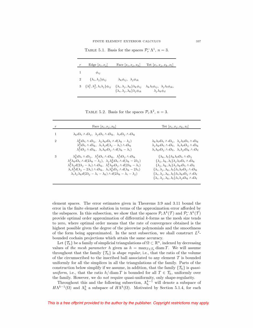
This is a free offprint provided to the author by the publisher. Copyright restrictions may apply.
FINITE ELEMENT EXTERIOR CALCULUS 337
Table 5.1. Basis for the spaces P−r Λ1, n = 3.
r Edge [xi, xj ] Face [xi, xj , xk] Tet [xi, xj , xk, xl]
1 φij
2 λi, λjφij λkφij , λjφik
3 λ2i , λ
2j , λiλjφij λi, λj , λkλkφij λkλlφij , λjλlφik,
λi, λj , λkλjφik λjλkφil
Table 5.2. Basis for the spaces PrΛ2, n = 3.
r Face [xi, xj , xk] Tet [xi, xj , xk, xl]
1 λkdλi ∧ dλj , λjdλi ∧ dλk, λidλj ∧ dλk
2 λ2kdλi ∧ dλj , λjλkdλi ∧ d(λk − λj) λkλldλi ∧ dλj , λjλldλi ∧ dλk
λ2jdλi ∧ dλk, λiλjd(λj − λi) ∧ dλk λjλkdλi ∧ dλl, λiλldλj ∧ dλk
λ2i dλj ∧ dλk, λiλkdλj ∧ d(λk − λi) λiλkdλj ∧ dλl, λiλjdλk ∧ dλl
3 λ3kdλi ∧ dλj , λ3
jdλi ∧ dλk, λ3i dλj ∧ dλk λk, λlλkλldλi ∧ dλj
λ2jλkdλi ∧ d(2λk − λj), λjλ2
kdλi ∧ d(λk − 2λj) λj , λk, λlλjλldλi ∧ dλk
λ2iλjd(2λj − λi) ∧ dλk, λ2
i λkdλj ∧ d(2λk − λi) λj , λk, λlλjλkdλi ∧ dλl
λiλ2jd(λj − 2λi) ∧ dλk, λiλ
2kdλj ∧ d(λk − 2λi) λi, λj , λk, λlλiλldλj ∧ dλk
λiλjλkd(2λj − λi − λk) ∧ d(2λk − λi − λj) λi, λj , λk, λlλiλkdλj ∧ dλl
λi, λj , λk, λlλiλjdλk ∧ dλl
element spaces. The error estimates given in Theorems 3.9 and 3.11 bound theerror in the finite element solution in terms of the approximation error afforded bythe subspaces. In this subsection, we show that the spaces PrΛ
k(T ) and P−r Λk(T )
provide optimal order approximation of differential k-forms as the mesh size tendsto zero, where optimal order means that the rate of convergence obtained is thehighest possible given the degree of the piecewise polynomials and the smoothnessof the form being approximated. In the next subsection, we shall construct L2-bounded cochain projections which attain the same accuracy.
Let Th be a family of simplicial triangulations of Ω ⊂ Rn, indexed by decreasingvalues of the mesh parameter h given as h = maxT∈Th
diamT . We will assumethroughout that the family Th is shape regular, i.e., that the ratio of the volumeof the circumscribed to the inscribed ball associated to any element T is boundeduniformly for all the simplices in all the triangulations of the family. Parts of theconstruction below simplify if we assume, in addition, that the family Th is quasi-uniform, i.e., that the ratio h/ diamT is bounded for all T ∈ Th, uniformly overthe family. However, we do not require quasi-uniformity, only shape-regularity.
Throughout this and the following subsection, Λk−1h will denote a subspace of
HΛk−1(Ω) and Λkh a subspace of HΛk(Ω). Motivated by Section 5.1.4, for each

This is a free offprint provided to the author by the publisher. Copyright restrictions may apply.
338 D. N. ARNOLD, R. S. FALK, AND RAGNAR WINTHER
r = 0, 1, . . . , we consider the following possible pairs of spaces:
(74) Λk−1h =
⎧⎪⎨⎪⎩Pr+1Λ
k−1(T )
or
P−r+1Λ
k−1(T )
⎫⎪⎬⎪⎭ , Λkh =
⎧⎪⎨⎪⎩P−r+1Λ
k(T )
or
PrΛk(T ) (if r > 0)
⎫⎪⎬⎪⎭ .
Note that Λkh contains all polynomials of degree r, but not r+1 in each case. As we
have seen in Section 5.2, the degrees of freedom define canonical projection opera-tors Ih = Ikh mapping CΛk(Ω) boundedly to Λk
h and commuting with the exteriorderivative. However, the operators Ih do not extend boundedly to all of L2Λk(Ω),or even to HΛk(Ω) and so do not fulfill the requirements of bounded cochain pro-jections of the abstract theory developed in Section 3. In this subsection, we willdescribe the Clement interpolant, which is a modification of the canonical projec-tion which is bounded on L2Λk and can be used to establish the approximationproperties of the finite element space. However, the Clement interpolant is nota projection and does not commute with the exterior derivative. So in the nextsubsection we construct a further modification which regains these properties andmaintains the approximation properties of the Clement interpolant.
The difficulty with the canonical interpolation operators Ih is that they make useof traces onto lower-dimensional simplexes, and as a consequence, they cannot beextended boundedly to L2Λk(Ω) (except for k = n). The Clement interpolant [34]is a classical tool of finite element theory developed to overcome this problem in thecase of 0-forms. To define this operator (for general k), we need some additionalnotation. For any f ∈ ∆(Th), we let Ωf ⊂ Ω be the union of elements containingf :
Ωf =⋃
T |T ∈ Th, f ∈ ∆(T ),
and let Pf : L2Λk(Ωf ) → PrΛk(Ωf ) be the L2 projection onto polynomial k-forms
of degree at most r. For ω ∈ L2Λk(Ω), we determine the Clement interpolant
Ihω := Ikhω ∈ Λkh by specifying φ(Ihω) for each degree of freedom φ of the space
Λkh; see Section 5.2. Namely, if φ is a degree of freedom for Λk
h associated tof ∈ ∆(Th), we take
φ(Ihω) = φ(Pfωf ),
where ωf = ω|Ωf.
The Clement interpolant is local in the sense that for any T ∈ Th, Ihω|T isdetermined by ω|T∗ , where T ∗ =
⋃Ωf | f ∈ ∆(T ). In fact, by scaling, as in [8,
Section 5.3], for example, it can be seen that
‖Ihω‖L2Λk(T ) ≤ c0∑
f∈∆(T )
‖Phω‖L2Λk(Ωf ) ≤ c1‖ω‖L2Λk(T∗),
where the constants c0, c1 may depend on the polynomial degree r and the di-mension n, but are independent of T ∈ Th and h, thanks to the shape regu-larity assumption. Therefore, the Clement interpolant is uniformly bounded inL(L2Λk(Ω), L2Λk(Ω)):
‖Ihω‖L2Λk(Ω) ≤ c2‖ω‖L2Λk(Ω)
(with the constant independent of h).
This is a free offprint provided to the author by the publisher. Copyright restrictions may apply.
FINITE ELEMENT EXTERIOR CALCULUS 339
Another key property of the Clement interpolant is that it preserves polynomialslocally in the sense that Ihω|T = ω|T if ω ∈ PrΛ
k(T ∗). It is then standard, usingthe Bramble–Hilbert lemma [23] and scaling, to obtain the following error estimate.
Theorem 5.8. Assume that Λkh is either P−
r+1Λk(Th), or, if r ≥ 1, PrΛ
k(Th).Then there is a constant c, independent of h, such that the Clement interpolantIkh : L2Λk(Ω) → Λk
h satisfies the bound
‖ω − Ikhω‖L2Λk(Ω) ≤ chs|ω|HsΛk(Ω), ω ∈ HsΛk(Ω),
for 0 ≤ s ≤ r + 1.
Note that the estimate implies that any sufficiently smooth k-form is approx-imated by elements Λk
h with order O(hr+1) in L2. Since the polynomial spacesused to construct Λk
h contain PrΛk but not Pr+1Λ
k, this is the optimal order ofapproximation.
5.5. Bounded cochain projections. The Clement interpolant Ih is both uni-formly bounded in L2 and gives optimal error bounds for smooth functions. How-ever, it is not a bounded cochain projection in the sense of the theory of Section3. Indeed, it is neither a projection operator—it does not leave Λk
h invariant—nordoes it commute with the exterior derivative. Therefore, to construct boundedcochain projections, we consider another modification of the canonical projectionIh, in which the operator Ih is combined with a smoothing operator.
This construction, key ingredients of which were contributed by Schoberl [79]and Christiansen [31], was discussed in detail in [8] (where it was called a smoothedprojection), under the additional assumption that the family of triangulations This quasi-uniform, and then in [32] in the general shape regular case. Therefore, wewill just give a brief outline of this construction here.
Let Λkh be one of the spaces P−
r+1Λk(Th) or, if r ≥ 1, PrΛ
k(Th), and let Ih :
CΛk(Ω) → Λkh be the corresponding canonical interpolant. To define an appropriate
smoothing operator, we let ρ : Rn → R be a nonnegative smooth function withsupport in the unit ball and with integral equal to one. In the quasi-uniform case,we utilize a standard convolution operator of the form
ω →∫|y|≤1
ρ(y)ω(x+ δy) dy,
mapping L2Λk(Ω) into C∞Λk(Ω), where the domain Ω ⊃ Ω is sufficiently largeso that the convolution operator is well defined. We set the smoothing parameterδ = εh, where the proportionality constant ε > 0 is a parameter to be chosen. Inthe more general shape regular case, we need to generalize this operator slightly.As in [32], we introduce a Lipschitz continuous function gh : Ω → R+, with Lips-chitz constant bounded uniformly in h, such that gh(x) is uniformly equivalent todiamT for T ∈ Th and x ∈ T . Hence, gh|T approximates diamT . The appropriate
smoothing operator in the general case, mapping L2Λk(Ω) into CΛk(Ω), is nowgiven by
ω →∫|y|≤1
ρ(y)((Φεyh )∗ω)x dy,
where the map Φεyh : Rn → Rn is defined by
Φεyh (x) = x+ εgh(x)y.

This is a free offprint provided to the author by the publisher. Copyright restrictions may apply.
340 D. N. ARNOLD, R. S. FALK, AND RAGNAR WINTHER
Since this smoothing operator is defined as an average of pullbacks, it will indeedcommute with the exterior derivative. By combining it with an appropriate exten-sion operator E : L2Λk(Ω) → L2Λk(Ω), constructed such that it commutes with theexterior derivative, we obtain an operator Rε
h : L2Λk(Ω) → CΛk(Ω). The operatorQε
h = Ih Rεh maps L2Λk(Ω) into Λk
h and commutes with the exterior derivative.Furthermore, for each ε > 0, the operators Qε
h are bounded in L2, uniformly in h.However, the operator Qε
h is not invariant on the subspace Λkh. The remedy to
fix this is to establish that the operators Qεh|Λk
h: Λk
h → Λkh converge to the identity
in the L2 operator norm as ε tends to zero, uniformly in h. Therefore, for a fixedε > 0, taken sufficiently small, this operator has an inverse Jε
h : Λkh → Λk
h. Thedesired projection operator, πh = πk
h, is now given as πh = Jεh Qε
h. The operatorsπh are uniformly bounded with respect to h as operators in L(L2Λk(Ω), L2Λk(Ω)).Furthermore, since they are projections onto Λk
h, we obtain
(75) ‖ω − πhω‖L2Λk(Ω) ≤ infµ∈Λk
h
‖(I − πh)(ω − µ)‖L2Λk(Ω).
Based on these considerations, we obtain the following theorem. Cf. [8, Theorem5.6] and [32, Corollary 5.3].
Theorem 5.9. 1. Let Λkh be one of the spaces P−
r+1Λk(Th) or, if r ≥ 1, PrΛ
k(Th)and πk
h : L2Λk(Ω) → Λkh the smoothed projection operator constructed above. Then
πkh is a projection onto Λk
h and satisfies
‖ω − πkhω‖L2Λk(Ω) ≤ chs‖ω‖HsΛk(Ω), ω ∈ HsΛk(Ω),
for 0 ≤ s ≤ r + 1. Moreover, for all ω ∈ L2Λk(Ω), πkhω → ω in L2 as h → 0.
2. Let Λkh be one of the spaces PrΛ
k(Th) or P−r Λk(Th) with r ≥ 1. Then
‖d(ω − πkhω)‖L2Λk(Ω) ≤ chs‖dω‖HsΛk(Ω), ω ∈ HsΛk(Ω),
for 0 ≤ s ≤ r.3. Let Λk−1
h and Λkh be taken as in (74) and let πk−1
h and πkh be the corresponding
smoothed projections. Then dπk−1h = πk
hd.
Proof. We have already established that the πkh are uniformly bounded projections
which commute with d. The error estimate in the first statement of the theoremthen follows from (75). Statement 2 follows from 1 and 3.
5.6. Approximation of the de Rham complex and the Hodge Laplacian.Let Λn
h be the space of piecewise polynomial n-forms of degree at most s for somenonnegative integer s. We showed in Section 5.2 that there are 2n−1 distinct discretede Rham complexes
(76) 0 → Λ0h
d−→ Λ0h
d−→ · · · d−→ Λnh → 0,
with each of the mappings Λk−1h
d−→ Λkh being of the form (73) for an appropriate
choice of s. Making use of the bounded projections, we obtain in each case acommuting diagram
0 →HΛ0(Ω)d−−−−→ HΛ1(Ω)
d−−−−→ · · · d−−−−→ HΛn(Ω) → 0πh
πh
πh
0 → Λ0h
d−−−−→ Λ1h
d−−−−→ · · · d−−−−→ Λnh → 0.

This is a free offprint provided to the author by the publisher. Copyright restrictions may apply.
FINITE ELEMENT EXTERIOR CALCULUS 341
Thus the projections give a cochain projection from the de Rham complex tothe discrete de Rham complex and so induce a surjection on cohomology. Sincelimh→0 ‖ω−πhw‖HΛk(Ω) = 0, we can use Theorem 3.4 (with V = HΛ and Vh = Λh)to see immediately that for h sufficiently small, this is in each case an isomorphismon cohomology.
The simplest finite element de Rham complex is the complex of Whitney forms,
(77) 0 → P−1 Λ0(Th)
d−→ P−1 Λ1(Th)
d−→ · · · d−→ P−1 Λn(Th) → 0.
Via the basic Whitney forms φf , the space P−1 Λk(Th) is isomorphic to the space
of simplicial cochains of dimension k associated to the triangulation Th. In thisway, the complex (77) of Whitney forms is isomorphic, as a cochain complex, tothe simplicial cochain complex, and its cohomology is isomorphic to the simplicialcohomology of Ω. Thus Theorem 3.4, when applied to the Whitney forms, givesan isomorphism between the de Rham cohomology and simplicial cohomology fora sufficiently fine triangulation. Since the simplicial cohomology is independent ofthe triangulation (being isomorphic to the singular cohomology), for the complexof Whitney forms, the isomorphism on cohomology given by Theorem 3.4 holds forany triangulation, not just one sufficiently fine. This proves de Rham’s theorem onthe equality of de Rham and simplicial cohomology.
For all of the discrete complexes (76), as for the Whitney forms, the cohomologyis independent of the triangulation (and equal to the de Rham cohomology). To seethis, following [31], we consider the Whitney forms complex (77) as a subcomplexof (76). The canonical projections Ih define cochain projections. Note that the Ihare defined on the finite element spaces Λk
h, because all of the trace moments theyrequire are single-valued on Λk
h. From the commuting diagram
0 → Λ0h
d−−−−→ Λ1h
d−−−−→ · · · d−−−−→ Λnh → 0Ih
Ih
Ih
0 →P−1 Λ0(Th)
d−−−−→ P−1 Λ1(Th)
d−−−−→ · · · d−−−−→ P−1 Λn(Th)→ 0,
we conclude that the cohomology of the top row, which we have already seen to bean image of the de Rham cohomology, maps onto the cohomology of the bottomrow, which is isomorphic to the de Rham cohomology. Hence the dimensions ofall the corresponding cohomology groups are equal and both cochain projectionsinduce an isomorphism on cohomology.
Consider now the numerical solution of the Hodge Laplacian problem (59). We
approximate this by a Galerkin method: Find σh ∈ Λk−1h , uh ∈ Λk
h, and ph ∈ Hkh
such that〈σh, τ 〉 − 〈dτ, uh〉 = 0, τ ∈ Λk−1
h ,
〈dσh, v〉+ 〈duh, dv〉+ 〈v, ph〉 = 〈f, v〉, v ∈ Λkh,
〈uh, q〉 = 0, q ∈ Hkh.
For the finite element spaces, we may choose Λk−1h and Λk
h to be any of the pairs
given in (74). We have verified that d maps Λk−1h into Λk
h and this map can beextended to a full subcomplex of the de Rham complex admitting a bounded cochainprojection. Therefore we may combine the error estimates derived in the abstractsetting in Sections 3.5 and 3.6 and approximation estimates from Section 5.5 toobtain convergence and rates of convergence. The rates of convergence are limited

This is a free offprint provided to the author by the publisher. Copyright restrictions may apply.
342 D. N. ARNOLD, R. S. FALK, AND RAGNAR WINTHER
by three factors: (1) the smoothness of the data f , (2) the amount of ellipticregularity (determined by the smoothness of the domain), and (3) the degree ofcomplete polynomials contained in the finite element shape functions. Specifically,from Theorem 3.11 we get the following result. Assume that the regularity estimate
‖u‖Ht+2(Ω) + ‖p‖Ht+2(Ω) + ‖du‖Ht+1(Ω) + ‖σ‖Ht+1(Ω) + ‖dσ‖Ht(Ω) ≤ C‖f‖Ht(Ω)
holds for 0 ≤ t ≤ tmax. Then for 0 ≤ s ≤ tmax the following estimates hold:
‖d(σ − σh)‖ ≤ Chs‖f‖Hs(Ω), if s ≤ r + 1,
‖σ − σh‖ ≤ Chs+1‖f‖Hs(Ω), if
s ≤ r + 1, Λk−1
h = Pr+1Λk−1(T ),
s ≤ r, Λk−1h = P−
r+1Λk−1(T ),
‖d(u− uh)‖ ≤ Chs+1‖f‖Hs(Ω), if
s ≤ r, Λk
h = P−r+1Λ
k(T ),
s ≤ r − 1, Λkh = PrΛ
k(T ),
‖u− uh‖+ ‖p− ph‖ ≤Ch‖f‖, Λk
h = P−1 Λk(T ),
Chs+2‖f‖Hs(Ω) if s ≤ r − 1, otherwise.
Thus, the error in each case is the optimal order allowed by the subspace if we havesufficient elliptic regularity.
Concerning the eigenvalue problem, applying Theorem 3.21, we immediatelyobtain the following error estimate:
|λ− λh| ≤ Ch2s+2‖u‖2Hs(Ω), 0 ≤ s ≤ r − 1.
This estimate does not apply in case Λkh = P−
1 Λk(T ), i.e., the Whitney forms. Inthat case, we get the estimate:
|λ− λh| ≤Ch‖u‖2,Ch2‖u‖‖u‖H1(Ω).
6. Variations of the de Rham complex
In Sections 4 and 5, we applied the abstract theory of Section 3 to the Hilbertcomplex obtained by choosing W k to be L2Λk(Ω) and dk to be the exterior de-rivative with domain V k = HΛk(Ω). This led to finite element approximations ofcertain boundary value problems for the Hodge Laplacian, and a variety of relatedproblems (B and B∗ problems, eigenvalue problems). In this section, we showhow some small variations of these choices lead to methods for important relatedproblems, namely generalizations of the Hodge Laplacian with variable coefficientsand problems with essential boundary conditions.
6.1. Variable coefficients. In this section, dk is again taken to be the exteriorderivative with domain V k = HΛk(Ω) and W k is again taken to be the space L2Λk,but W k is furnished with an inner product which is equivalent to, but not equal to,the standard L2Λk inner product. Specifically, we let ak : W k → W k be a bounded,symmetric, positive definite operator and choose
〈u, v〉Wk = 〈aku, v〉L2Λk .
With this choice, we can check that d∗k = (dk−1)∗ is given by
d∗ku = (ak−1)−1δkaku,

This is a free offprint provided to the author by the publisher. Copyright restrictions may apply.
FINITE ELEMENT EXTERIOR CALCULUS 343
with the domain of d∗k given by
V ∗k = u ∈ L2Λk(Ω) | aku ∈ H∗Λk(Ω) = (ak)−1H∗Λk(Ω).
The harmonic forms are then
Hk = Z
k ∩ Z∗k = u ∈ HΛk ∩ (ak)−1H∗Λk | du = 0, δaku = 0 .
The Hodge Laplacian d∗du+ dd∗u is now realized as
d(ak−1)−1δaku+ (ak)−1δak+1du.
As an example of the utility of this generalization, we consider the B∗1 eigenvalue
problem in three dimensions. We take a1 = ε and a2 = µ−1, where ε and µ aresymmetric positive definite 3× 3 matrix fields. Then the B∗
1 eigenvalue problem is
curlµ−1 curlu = λεu.
This is the standard Maxwell eigenvalue problem, where ε is the dielectric tensorof the material and µ is its magnetic permeability. These are scalar for an isotropicmaterial, but given by matrices in general. They are constant for a homogeneousmaterial, but vary if the material is not constant across the domain.
We notice that the Hilbert complex in this case is exactly the de Rham complex(52), except that the spaces are furnished with different, but equivalent, inner prod-ucts. Thus the finite element de Rham subcomplexes we constructed in Section 5apply for this problem and satisfy the subcomplex and bounded cochain projectionproperties. In other words, the same finite element spaces which were developed forthe constant coefficient Hodge Laplacian can be applied equally well for variablecoefficient problems.
6.2. The de Rham complex with boundary conditions. For another impor-tant application of the abstract theory of Section 3, we again choose W k = L2Λk(Ω)and dk to be the exterior derivative, but this time we take its domain V k to bethe space HΛk(Ω). This space is dense in W k and is a closed subspace of HΛk,so is complete, and hence d is again a closed operator with this domain. Thus weobtain the following complex of Hilbert spaces, called the de Rham complex withboundary conditions:
(78) 0 → HΛ0(Ω)d−→ HΛ1(Ω)
d−→ · · · d−→ HΛn(Ω) → 0.
In Section 4.2, we used the fact that HΛk ∩ H∗Λk is compactly included in L2Λk.Replacing k by n − k and applying the Hodge star operator, we conclude theanalogous result, that HΛk ∩ H∗Λk is compactly included in L2Λk. Then, justas in Section 4.2, all the results of Section 3 apply to the de Rham complex withboundary conditions. In particular, we have the Hodge decomposition of L2Λk andof HΛk, the Poincare inequality, well-posedness of the mixed formulation of theHodge Laplacian, and all the approximation results established in Sections 3.3–3.6.
We denote the spaces of k-cocycles, k-coboundaries, and harmonic k-forms as
Zk = ω ∈ HΛk | dω = 0 , B
k = dη | η ∈ HΛk−1 ,H
k = ω ∈ Zk | 〈ω, µ〉 = 0, µ ∈ B
k .
Now, from (53), we have that
(79) 〈dω, µ〉 = 〈ω, δµ〉, ω ∈ HΛk−1, µ ∈ H∗Λk.

This is a free offprint provided to the author by the publisher. Copyright restrictions may apply.
344 D. N. ARNOLD, R. S. FALK, AND RAGNAR WINTHER
Therefore
Bk⊥L2 := ω ∈ L2Λk | 〈ω, dη〉 = 0 ∀η ∈ HΛk−1 = ω ∈ H∗Λk | δω = 0 .
This gives a concrete characterization of the harmonic forms analogous to (58):
(80) Hk = ω ∈ HΛk(Ω) ∩H∗Λk(Ω) | dω = 0, δω = 0.
Now, from (54), (55), and (50), the Hodge star operator maps the set of ω ∈ HΛn−k
with dω = 0 isomorphically onto the set of µ ∈ H∗Λk with δµ = 0, and it mapsthe set of ω ∈ H∗Λn−k with δω = 0 isomorphically onto the set of µ ∈ HΛk withdµ = 0. Comparing (58) and (80), we conclude that the Hodge star operator maps
Hn−k isomorphically onto Hk. This isomorphism is called Poincare duality. Inparticular, dim Hk is the (n− k)th Betti number of Ω.
Finally, from (79), we can characterize d∗, the adjoint of the exterior derivative
d viewed as an unbounded operator L2Λk−1 → L2Λk with domain HΛk. Namely,in this case, d∗ has domain H∗Λk and coincides with the operator δ defined in (50).By contrast, when we took the domain of d to be all of HΛk, the domain of d∗
turned out to be the smaller space H∗Λk.We now consider the Hodge Laplacian problem given in the abstract case by
(18). In this case, we get that (σ, u, p) ∈ HΛk−1 × HΛk × Hk is a solution if andonly if
σ = δu, dσ + δdu = f − p in Ω,(81)
trσ = 0, tru = 0 on ∂Ω,(82)
u ⊥ Hk.(83)
Note that now both boundary conditions are essential in the sense that they areimplied by membership in the spaces HΛk−1 and HΛk where the solution is sought,rather than by the variational formulation.
To make things more concrete, we restrict to a domain Ω ⊂ R3 and consider theHodge Laplacian for k-forms, k = 0, 1, 2, and 3. We also discuss the B∗ and B
problems given by (19) and (20) for each k. Again we have
d0 = grad, d1 = curl, d2 = div,
and the de Rham complex (78) is now realized as
0 → H1(Ω)grad−−−→ H(curl; Ω)
curl−−→ H(div; Ω)div−−→ L2(Ω) → 0,
where
H(curl; Ω) = u : Ω → R3 |u ∈ L2, curlu ∈ L2, u× n = 0 on ∂Ω ,H(div; Ω) = u : Ω → R3 |u ∈ L2, div u ∈ L2, u · n = 0 on ∂Ω .
6.2.1. The Hodge Laplacian for k = 0. For k = 0, the boundary value problem(81)–(83) is the Dirichlet problem for the ordinary scalar Laplacian. The space
HΛ−1 is understood to be 0, so σ vanishes. The space H0 of harmonic 0-formsvanishes. The first differential equation of (81) vanishes, and the second givesPoisson’s equation
− div gradu = f in Ω.
This is a free offprint provided to the author by the publisher. Copyright restrictions may apply.
FINITE ELEMENT EXTERIOR CALCULUS 345
Similarly, the first boundary condition in (82) vanishes, while the second is theDirichlet condition u = 0 on ∂Ω. The side condition (83) is automatically satis-fied. Nothing additional is obtained by considering the split into the B∗ and B
subproblems, since the latter is trivial.
6.2.2. The Hodge Laplacian for k = 1. In this case the differential equations andboundary conditions are
(84)σ = − div u, gradσ + curl curlu = f − p in Ω,
σ = 0, u× n = 0 on ∂Ω,
which is a formulation of a boundary value problem for the vector Laplaciancurl curl− grad div. The solution is determined uniquely by the additional con-
dition that u be orthogonal to H1 = H2, i.e., those vector fields satisfying
curl p = 0, div p = 0 in Ω, p× n = 0 on ∂Ω.
The B∗1 problem (19) is defined for L2 vector fields f which are orthogonal to
both gradients of functions in H1(Ω) and the vector fields in H1. In that case, thesolution to (84) has σ = 0 and p = 0, while u satisfies
curl curlu = f, div u = 0 in Ω, u× n = 0 on ∂Ω.
The orthogonality condition u ⊥ H1 again determines the solution uniquely.Next we turn to the B1 problem. For source functions of the form f = gradF for
some F ∈ H1, (84) reduces to the problem of finding σ ∈ H1 and u ∈ B1 = grad H1
such that:
σ = − div u, gradσ = f in Ω.
The differential equations may be simplified to − grad div u = f and the conditionthat u ∈ B1 can be replaced by the differential equation curlu = 0 and the bound-
ary condition u× n = 0, together with orthogonality to H1. Now grad(σ − F ) = 0and σ − F = 0 on ∂Ω, so σ = F . Hence, we may rewrite the system as
− div u = F, curlu = 0 in Ω, u× n = 0 on ∂Ω,
which, again, has a unique solution subject to orthogonality to H1.
6.2.3. The Hodge Laplacian for k = 2. The differential equations and boundaryconditions are
σ = curlu, curlσ − grad div u = f − p in Ω,
σ × n = 0, u · n = 0 on ∂Ω.
This is again a formulation of a boundary value problem for the vector Laplaciancurl curl− grad div, but with different boundary conditions than for (84), and thistime stated in terms of two vector variables, rather than one vector and one scalar.
This time uniqueness is obtained by imposing orthogonality to H2 = H1, the spaceof vector fields satisfying
curl p = 0, div p = 0 in Ω, p · n = 0 on ∂Ω.
The B∗2 problem arises for source functions of the form f = gradF for some
F ∈ H1 which we may take to have integral 0. We find σ = 0, and u solves
− div u = F, curlu = 0 in Ω, u · n = 0 on ∂Ω,

This is a free offprint provided to the author by the publisher. Copyright restrictions may apply.
346 D. N. ARNOLD, R. S. FALK, AND RAGNAR WINTHER
i.e., the same differential equation as for B1, but with different boundary conditions
and, of course, now uniqueness is determined by orthogonality to H2.If div f = 0, f · n = 0 on ∂Ω, and f ⊥ H2, we get the B2 problem for which the
differential equations are σ = curlu, curlσ = f and the condition div u = 0 arisingfrom the membership of u in B2. Thus u solves
curl curlu = f, div u = 0 in Ω, u · n = 0 on ∂Ω,
the same differential equation as for B∗1, but with different boundary conditions.
6.2.4. The Hodge Laplacian for k = 3. The space H3 consists of the constants (or, ifΩ is not connected, of functions which are constant on each connected component).The Hodge Laplacian problem is
σ = − gradu, div σ = f − p in Ω, σ · n = 0 on ∂Ω,
∫Ω
u q dx = 0, q ∈ H3,
which is the Neumann problem for Poisson’s equation, where the (piecewise) con-stant p is required for there to exist a solution and the final condition fixes a uniquesolution.
7. The elasticity complex
In this section, we present another complex, which we call the elasticity complex,and apply it to the development of numerical methods for linear elasticity. Incontrast to the other examples presented above, the elasticity complex is not asimple variant of the de Rham complex, and, in particular, it involves a differentialoperator of second order. However, the two complexes are related in a subtlemanner, via a construction known as the Bernstein–Bernstein–Gelfand resolution,explained for example in [8, 9, 43] and the references given there.
The equations of elasticity are of great importance in modeling solid structures,and the need to solve them in engineering applications was probably the primaryreason for the development of the finite element method in the 1960s. The sim-plest finite element methods for elasticity are based on displacement approaches, inwhich the displacement vector field is characterized as the minimizer of an elasticenergy functional. The design and analysis of displacement finite element meth-ods is standard and discussed in many textbooks (e.g., [33]). However, for moregeneral material models, arising, for example, for incompressible materials or someviscoelastic or plastic materials, the displacement method is either not feasible orperforms poorly, and a mixed approach, in which the elastic stress and the dis-placement are taken as unknowns, is the natural alternative. In fact, mixed finiteelement methods for elasticity were proposed in the earliest days of finite elements[51], and stable finite elements for the mixed formulation of elasticity have beensought for over four decades. These proved very elusive. Indeed, one of the motiva-tions of the pioneering work of Raviart and Thomas [76] on mixed finite elementsfor the Laplacian, was the hope that the solution to this easier problem would pavethe way to such elements for elasticity, and there were many attempts to generalizetheir elements to the elasticity system [4, 5, 63, 80, 81, 82]. However, it was notuntil 2002 that the first stable mixed finite elements for elasticity using polynomialshape functions were discovered by two of the present authors [11], based on tech-niques and insights from the then nascent finite element exterior calculus. See also[7]. They developed and analyzed a family of methods for plane (two-dimensional)
This is a free offprint provided to the author by the publisher. Copyright restrictions may apply.
FINITE ELEMENT EXTERIOR CALCULUS 347
elasticity. The basic elements in the family involve a space of shape functions inter-mediate between quadratics and cubics for the stress, with 24 degrees of freedom,while the displacement field consists of the complete space of piecewise linear vectorfields, without continuity constraints. It is these elements we will describe here.
The plane elasticity elements of [11] were generalized to three dimensions in[3]. See also [1]. These elements are, however, quite complicated (162 degrees offreedom per tetrahedron for the stress). A much more promising approach involves avariant Hilbert complex for elasticity, the elasticity complex with weak symmetry.In [8] and [9], stable families of finite elements are derived for this formulationin n dimensions, again using techniques from the finite element exterior calculus.For the lowest-order stable elements, the stress space is discretized by piecewiselinears with just 12 degrees of freedom per triangle in two dimensions, 36 pertetrahedron in three dimensions, while the other variables are approximated bypiecewise constants.
7.1. The elasticity system. The equations of linear elasticity arise as a systemconsisting of a constitutive equation and an equilibrium equation:
(85) Aσ = ε u, div σ = f in Ω.
Here the unknowns σ and u denote the stress and displacement fields engendered bya body force f acting on a linearly elastic body which occupies a region Ω ⊂ Rn. Theconstitutive equation posits a linear relationship between the linearized deformationor strains due to the displacement and the stresses. The equilibrium equation statesthat the stresses, which measure the internal forces in the body, are in equilibriumwith the externally applied force. The stress field σ takes values in the space S :=Rn×n
sym of symmetric matrices and the displacement field u takes values in V := Rn.The differential operator ε is the symmetric part of the gradient, the div operatoris applied row-wise to a matrix, and the compliance tensor A = A(x) : S → S is abounded and symmetric, uniformly positive definite operator reflecting the materialproperties of the body. If the body is clamped on the boundary ∂Ω of Ω, then theappropriate boundary condition for the system (85) is u = 0 on ∂Ω. For simplicity,this boundary condition will be assumed here.
The pair (σ, u) can alternatively be characterized as the unique critical point ofthe Hellinger–Reissner functional
I(τ, v) =
∫Ω
(12Aτ : τ + div τ · v − f · v
)dx.
The critical point is sought among τ ∈ H(div; Ω; S), the space of square-integrablesymmetric matrix fields with square-integrable divergence, and v ∈ L2(Ω;V), thespace of square-integrable vector fields. Equivalently, the pair (σ, u) ∈ H(div; Ω; S)×L2(Ω;V) is the unique solution to the weak formulation of the system (85):
(86)
∫Ω(Aσ : τ + div τ · u) dx = 0, τ ∈ H(div; Ω; S),∫
Ωdiv σ · v dx =
∫Ωf · v dx, v ∈ L2(Ω;V).
7.2. The elasticity complex and its discretization. The discretization of theproblem (86) is closely tied to the discretization of the elasticity complex. For atwo-dimensional domain Ω, the elasticity complex takes the form
(87) 0 →H2(Ω)J−−−−→ H(div; Ω; S)
div−−−−→ L2(Ω;R2)→ 0.

This is a free offprint provided to the author by the publisher. Copyright restrictions may apply.
348 D. N. ARNOLD, R. S. FALK, AND RAGNAR WINTHER
The operator J is a second-order differential operator mapping scalar fields intosymmetric matrix fields, namely the rotated Hessian
Jq =
(∂2yq −∂x∂yq
−∂x∂yq ∂2xq
)= O(grad grad q)OT , O =
(0 1−1 0
).
We now show that this complex is closed, i.e., that the range of the two operatorsJ and div are closed subspaces. The null space of J is just the space P1 of linearpolynomials, and we have ‖q‖H2 ≤ c‖Jq‖L2 for all q ∈ H2(Ω) with q ⊥ P1, whichimplies that the range of J is closed. We now show that div maps H(div; Ω; S)onto L2(Ω;R2), using the fact that the scalar-valued divergence maps H1(Ω;R2)onto L2(Ω). Given f ∈ L2(Ω;R2), the latter result implies the existence of τ ∈H1(Ω;R2×2) with div τ = f . This τ may not be symmetric. However, for anyv ∈ H1(Ω;R2), we let curl v denote the matrix with ith row equal to curl vi =(−∂vi/∂x2, ∂vi/∂x1). Then div(τ + curl v) = f and τ + curl v ∈ H(div; Ω; S) ifdiv v = τ21 − τ12. Thus div : H(div; Ω; S) → L2(Ω;R2) is indeed surjective. SettingW 0 = L2(Ω), W 1 = L2(Ω; S), and W 2 = L2(Ω;R2), we obtain a closed Hilbertcomplex with domain complex (87).
Now we describe only the simplest discretization from [11]. The space V 0h ⊂
V 0 = H2(Ω) is the finite element space whose shape functions on each triangleT are the quintic polynomials P5(T ) and whose degrees of freedom are the values,first derivatives and second derivatives at each vertex, together with the mean valueof the normal derivatives along each edge, which gives 21 = dimP5(T ) degrees offreedom per triangle. The resulting finite element space V 0
h is referred to in thefinite element literature as the Argyris space, and is easily seen to be containedin C1(Ω), and hence in H2(Ω). In fact, the Argyris space is in a certain sensethe simplest finite element space contained in C1(Ω). However, the Argyris spacedoes not coincide with the space of all C1 piecewise quintics (which is not a finiteelement space, as it cannot be defined via degrees of freedom). Elements of theArgyris space have extra smoothness at the vertices, where they are C2.
The space V 1h ⊂ V 1 = H(div; Ω; S) consists of those continuous piecewise cu-
bic symmetric matrix fields whose divergence is piecewise linear. The degrees offreedom determining an element σ ∈ V 1
h are
• the value of σ at each vertex,• the moments of degree 0 and 1 of the two normal components of σ on eachedge, and
• the moments of degree 0 of σ on each triangle.
Hence, the restriction of σ to a triangle T ∈ Th is uniquely determined by 24 degreesof freedom. Finally, the space V 2
h ⊂ V 2 = L2(Ω;R2) consists of all piecewise linearvector fields with respect to Th, without any imposed continuity. For degrees offreedom, we choose the moments of degrees 0 and 1 for each component on eachtriangle T . Using the degrees of freedom, we also define projections Ikhv ∈ V k
h
defined for sufficiently smooth v ∈ V k by φ(Ikhv) = φ(v) for all degrees of freedomφ.
It is straightforward to check that we have the subcomplex property JV 0h ⊂ V 1
h
and div V 1h ⊂ V 2
h and that the interpolation operators Ih := Ikh give a commuting

This is a free offprint provided to the author by the publisher. Copyright restrictions may apply.
FINITE ELEMENT EXTERIOR CALCULUS 349
diagram
(88)
0 →V 0 ∩ C2 J−−−−→ V 1 ∩ C0 div−−−−→ V 2 → 0
I0h
I1h
I2h
0 → V 0
hJ−−−−→ V 1
hdiv−−−−→ V 2
h → 0.
However, since I0h involves point values of the second derivative and I1h involvespoint values, these operators do not extend to bounded operators on the Hilbertspaces V 0 and V 1.
In order to apply the general theory of approximation of Hilbert complexesdeveloped in Section 3, we will modify the interpolation operators Ikh in (88) toobtain bounded cochain projections πk
h : W k → V kh for k = 0, 1, 2. As in Section 5.5,
the πkh will be obtained from Ikh via smoothing.
7.3. Bounded cochain projections for the elasticity complex. First, we de-fine an appropriate pullback of an affine map and show that it defines a cochain mapfor the elasticity sequence. Let F : Ω → Ω′ ⊂ R2 be an affine map, so that DF =DF (x) is a constant 2 × 2 matrix. Let B be the matrix B = det(DF )(DF )−1 =O(DF )TOT and define pullbacks F ∗ = F ∗
k : W k(Ω′) → W k(Ω) by
F ∗v = v F, v ∈ W 0(Ω′),
F ∗v = B(v F )BT , v ∈ W 1(Ω′),
F ∗v = det(DF )B(v F ), v ∈ W 2(Ω′).
It is straightforward to check that, as long as F is affine, F ∗ commutes with thedifferential operators J and div. In other words, we obtain the commuting diagram
0 →V 0(Ω′)J−−−−→ V 1(Ω′)
div−−−−→ V 2(Ω′) → 0
F∗ F∗
F∗
0 → V 0(Ω)J−−−−→ V 1(Ω)
div−−−−→ V 2(Ω) → 0.
To define a smoothing operator which maps W k into itself, we need to makethe assumption that the domain Ω is star-shaped with respect to some point in itsinterior (which we assume, without further loss of generality, to be the origin).We then let a = maxx∈∂Ω |x|−1 and define the dilation Fδ : R2 → R2 by Fδ(x) =x/(1 + aδ), δ > 0. Then Fδ maps the δ-neighborhood of Ω, Ωδ, into Ω and so F ∗
δ
maps L2(Ω) to L2(Ωδ). Composing with a standard mollification
v →∫|z|<1
ρ(z)v(x+ δz) dz,
we obtain a smoothing operator Rδ mapping W k into W k. Here ρ : R2 → R isa smooth, nonnegative function supported in the unit ball and with integral equalto one. This smoothing commutes with any differential operator with constantcoefficients, in particular with J and div.
The construction now proceeds as in Section 5.5, and we just give an outline ofit. For simplicity, we assume a quasi-uniform family of meshes, although extensionto general shape regular meshes could be made as in Section 5.5. Let ε > 0 be fixed.Define operators Qk
h : W k → W kh by Qk
h = Ikh Rεh. The operator Qkh maps W k
into V kh . In fact, it can be seen by a scaling argument that the operators Qk
h are

This is a free offprint provided to the author by the publisher. Copyright restrictions may apply.
350 D. N. ARNOLD, R. S. FALK, AND RAGNAR WINTHER
bounded as operators in L(W k,W k), uniformly in h. Furthermore, Qkh commutes
with J and div, i.e.,
(89) Q1h J = J Q0
h and Q2h div = div Q1
h.
However, the operators Qkh are not projections, since they do not restrict to the
identity on V kh . Therefore, we define the desired projections πk
h : W k → V kh as
πkh = (Qk
h|V kh)−1Qk
h. To justify this definition, we need to argue that (Qkh|V k
h)−1
exists. In fact, for ε sufficiently small, but fixed, (Qkh|V k
h)−1 is even uniformly
bounded in L(W kh ,W
kh ), where W k
h = V kh , but equipped with the norm of W k.
This follows from the fact that the operators Qkh|V k
hconverge to the identity with
ε in L(W kh ,W
kh ), uniformly in h, established by a scaling argument.
We conclude that if the parameter ε > 0 is fixed, but sufficiently small, thenthe operators πk
h are well defined and uniformly bounded with respect to h inL(W k,W k). Furthermore, the diagram
0 →V 0 J−−−−→ V 1 div−−−−→ V 2 → 0
πh
πh
πh
0 →V 0
hJ−−−−→ V 1
hdiv−−−−→ V 2
h → 0
commutes, as a consequence of (89).Thus, under the assumption of a star-shaped domain, we have established the
existence of bounded cochain projections and so the results of Section 3.4 apply tothe elasticity complex. This means that the corresponding Hodge Laplacians arewell-posed and that the discretizations are stable. In particular, using the spacesV 1h and V 2
h , we obtain a stable, convergent mixed discretization of the elasticityequations.
Remark. Stability and convergence of the mixed finite element method for elasticityusing the spaces V 1
h and V 2h described above is proven in [11] without restricting to
star-shaped domains. However, we do not know how to construct bounded cochainprojections without this restriction.
Acknowledgments
The authors would like to thank Marie Rognes for her help with some of thecomputations appearing in Section 2.3.
About the authors
Douglas Arnold is McKnight Presidential Professor of Mathematics at the Uni-versity of Minnesota and President of the Society for Industrial and Applied Mathe-matics (SIAM). He was a plenary speaker at the ICM in Beijing in 2002, a Guggen-heim Fellow in 2008–2009, and is a foreign member of the Norwegian Academy ofScience and Letters.
Richard Falk is a professor at Rutgers University. He has served both as Chairof the Department of Mathematics and Acting Dean of the Faculty of Arts andSciences and of the Graduate School and has co-organized the biannual “FiniteElement Circus” meetings of researchers on finite element methods since 1996.
Ragnar Winther is a professor at and director of the Centre of Mathematics forApplications at the University of Oslo, Norway. He is chairman of the board of the

This is a free offprint provided to the author by the publisher. Copyright restrictions may apply.
FINITE ELEMENT EXTERIOR CALCULUS 351
N.H. Abel Memorial Fund and was an invited speaker at the European Congressof Mathematics in Amsterdam in 2008.
References
1. Scot Adams and Bernardo Cockburn, A mixed finite element method for elasticity in threedimensions, J. Sci. Comput. 25 (2005), no. 3, 515–521. MR2221175 (2006m:65251)
2. C. Amrouche, C. Bernardi, M. Dauge, and V. Girault, Vector potentials in three-dimensionalnon-smooth domains, Math. Methods Appl. Sci. 21 (1998), 823–864. MR1626990 (99e:35037)
3. Douglas N. Arnold, Gerard Awanou, and Ragnar Winther, Finite elements for symmet-ric tensors in three dimensions, Math. Comp. 77 (2008), no. 263, 1229–1251. MR2398766(2009b:65291)
4. Douglas N. Arnold, Franco Brezzi, and Jim Douglas, Jr., PEERS: a new mixed finite elementfor plane elasticity, Japan J. Appl. Math. 1 (1984), 347–367. MR840802 (87h:65189)
5. Douglas N. Arnold, Jim Douglas, Jr., and Chaitan P. Gupta, A family of higher ordermixed finite element methods for plane elasticity, Numer. Math. 45 (1984), 1–22. MR761879(86a:65112)
6. Douglas N. Arnold, Richard S. Falk, and Ragnar Winther, Differential complexes and stabilityof finite element methods. I. The de Rham complex, Compatible Spatial Discretizations, IMAVol. Math. Appl., vol. 142, Springer, New York, 2006, pp. 24–46. MR2249344 (2008c:65296)
7. , Differential complexes and stability of finite element methods. II. The elasticity com-plex, Compatible Spatial Discretizations, IMA Vol. Math. Appl., vol. 142, Springer, New York,2006, pp. 47–67. MR2249345 (2008c:65307)
8. , Finite element exterior calculus, homological techniques, and applications, Acta Nu-mer. 15 (2006), 1–155. MR2269741 (2007j:58002)
9. , Mixed finite element methods for linear elasticity with weakly imposed symmetry,Math. Comp. 76 (2007), no. 260, 1699–1723 (electronic). MR2336264
10. , Geometric decompositions and local bases for spaces of finite element differentialforms, Comput. Methods Appl. Mech. Engrg. 198 (2009), 1660–1672. MR2517938
11. Douglas N. Arnold and Ragnar Winther, Mixed finite elements for elasticity, Numer. Math.92 (2002), 401–419. MR1930384 (2003i:65103)
12. Vladimir I. Arnold, Mathematical Methods of Classical Mechanics, Springer-Verlag, NewYork, 1978. MR0690288 (57:14033b)
13. Ivo Babuska, Error-bounds for finite element method, Numer. Math. 16 (1970/1971), 322–333.MR0288971 (44:6166)
14. Ivo Babuska and John Osborn, Eigenvalue problems, Handbook of Numerical Analysis, Vol.II, North-Holland, Amsterdam, 1991, pp. 641–787. MR1115240
15. Garth A. Baker, Combinatorial Laplacians and Sullivan-Whitney forms, Differential geometry(College Park, Md., 1981/1982), Progr. Math., vol. 32, Birkhauser, Boston, Mass., 1983, pp. 1–33. MR702525 (84m:58005)
16. Pavel B. Bochev and James M. Hyman, Principles of mimetic discretizations of differentialoperators, Compatible Spatial Discretizations, IMA Vol. Math. Appl., vol. 142, Springer, NewYork, 2006, pp. 89–119. MR2249347 (2007k:65161)
17. Daniele Boffi, A note on the de Rham complex and a discrete compactness property, Appl.Math. Lett. 14 (2001), 33–38. MR1793699 (2001g:65145)
18. , Compatible discretizations for eigenvalue problems, Compatible Spatial Discretiza-tions, IMA Vol. Math. Appl., vol. 142, Springer, New York, 2006, pp. 121–142. MR2249348(2007i:65084)
19. , Approximation of eigenvalues in mixed form, discrete compactness property, andapplication to hp mixed finite elements, Comput. Methods Appl. Mech. Engrg. 196 (2007),no. 37-40, 3672–3681. MR2339993 (2008e:65339)
20. Daniele Boffi, Franco Brezzi, and Lucia Gastaldi, On the problem of spurious eigenvalues inthe approximation of linear elliptic problems in mixed form, Math. Comp. 69 (2000), 121–140.MR1642801 (2000i:65175)
21. Alain Bossavit, Whitney forms: A class of finite elements for three-dimensional computationsin electromagnetism, IEE Trans. Mag. 135, Part A (1988), 493–500.
22. Raoul Bott and Loring W. Tu, Differential Forms in Algebraic Topology, Graduate Texts inMathematics, vol. 82, Springer, New York, 1982. MR658304 (83i:57016)

This is a free offprint provided to the author by the publisher. Copyright restrictions may apply.
352 D. N. ARNOLD, R. S. FALK, AND RAGNAR WINTHER
23. James H. Bramble and Stephen R. Hilbert, Estimation of linear functionals on Sobolev spaceswith application to Fourier transforms and spline interpolation, SIAM J. Numer. Anal. 7(1970), 112–124. MR0263214 (41:7819)
24. Franco Brezzi, On the existence, uniqueness and approximation of saddle-point problems aris-ing from Lagrangian multipliers, Rev. Francaise Automat. Informat. Recherche OperationnelleSer. Rouge 8 (1974), 129–151. MR0365287 (51:1540)
25. Franco Brezzi and Klaus-Jurgen Bathe, A discourse on the stability conditions for mixed finite
element formulations, Comput. Methods Appl. Mech. Engrg. 82 (1990), 27–57. MR1077650(92b:65085)
26. Franco Brezzi, Jim Douglas, Jr., and L. D. Marini, Two families of mixed finite elements forsecond order elliptic problems, Numer. Math. 47 (1985), 217–235. MR799685 (87g:65133)
27. Franco Brezzi, Konstantin Lipnikov, and Mikhail Shashkov, Convergence of the mimetic finitedifference method for diffusion problems on polyhedral meshes, SIAM J. Numer. Anal. 43(2005), no. 5, 1872–1896 (electronic). MR2192322 (2006j:65311)
28. Jochen Bruning and Matthias Lesch, Hilbert complexes, J. Funct. Anal. 108 (1992), no. 1,88–132. MR1174159 (93k:58208)
29. Jules G. Charney, Ragnar Fjortoft, and John von Neumann, Numerical integration of thebarotropic vorticity equation, Tellus 2 (1950), 237–254. MR0042799 (13:164f)
30. Jeffrey Cheeger, Analytic torsion and the heat equation, Ann. of Math. (2) 109 (1979), no. 2,259–322. MR528965 (80j:58065a)
31. Snorre H. Christiansen, Stability of Hodge decompositions in finite element spaces of differ-ential forms in arbitrary dimension, Numer. Math. 107 (2007), no. 1, 87–106. MR2317829(2008c:65318)
32. Snorre H. Christiansen and Ragnar Winther, Smoothed projections in finite element exteriorcalculus, Math. Comp. 77 (2008), no. 262, 813–829. MR2373181 (2009a:65310)
33. Philippe G. Ciarlet, The finite element method for elliptic problems, North-Holland PublishingCo., Amsterdam, 1978. MR0520174 (58:25001)
34. Philippe Clement, Approximation by finite element functions using local regularization,Rev. Francaise Automat. Informat. Recherche Operationnelle Ser. Rouge, RAIRO AnalyseNumerique 9 (1975), 77–84. MR0400739 (53:4569)
35. Martin Costabel, A coercive bilinear form for Maxwell’s equations, J. Math. Anal. Appl. 157(1991), 527–541. MR1112332 (92c:35113)
36. Richard Courant, Kurt Friedrichs, and Hans Lewy, Uber die partiellen Differenzengleichungender mathematischen Physik, Math. Ann. 100 (1928), no. 1, 32–74. MR1512478
37. Leszek Demkowicz, Peter Monk, Leon Vardapetyan, and Waldemar Rachowicz, de Rhamdiagram for hp finite element spaces, Comput. Math. Appl. 39 (2000), 29–38. MR1746160(2000m:78052)
38. Mathieu Desbrun, Anil N. Hirani, Melvin Leok, and Jerrold E. Marsden, Discrete exteriorcalculus, 2005, available from arXiv.org/math.DG/0508341.
39. Jozef Dodziuk, Finite-difference approach to the Hodge theory of harmonic forms, Amer. J.Math. 98 (1976), no. 1, 79–104. MR0407872 (53:11642)
40. Jozef Dodziuk and V. K. Patodi, Riemannian structures and triangulations of manifolds, J.Indian Math. Soc. (N.S.) 40 (1976), no. 1-4, 1–52. MR0488179 (58:7742)
41. Jim Douglas, Jr. and Jean E. Roberts, Global estimates for mixed methods for second orderelliptic equations, Math. Comp. 44 (1985), 39–52. MR771029 (86b:65122)
42. Patrick Dular and Christophe Geuzaine, GetDP: A general environment for the treatment ofdiscrete problems, http://geuz.org/getdp/.
43. Michael Eastwood, A complex from linear elasticity, Rend. Circ. Mat. Palermo (2) Suppl.(2000), no. 63, 23–29. MR1758075 (2001j:58033)
44. Anders Logg et al., The FEniCS project, http://www.fenics.org.45. Daniel White et al., EMSolve: Unstructured grid computational electromagnetics using mixed
finite element methods, https://www-eng.llnl.gov/emsolve/emsolve_home.html.46. Wolfgang Bangerth et al., deal.II: A finite element differential equations analysis library,
http://www.dealii.org.47. Lawrence C. Evans, Partial differential equations, Graduate Studies in Mathematics, vol. 19,
American Mathematical Society, Providence, RI, 1998. MR1625845 (99e:35001)48. Richard S. Falk and John E. Osborn, Error estimates for mixed methods, RAIRO Anal.
Numer. 14 (1980), 249–277. MR592753 (82j:65076)

This is a free offprint provided to the author by the publisher. Copyright restrictions may apply.
FINITE ELEMENT EXTERIOR CALCULUS 353
49. Herbert Federer, Geometric Measure Theory, Vol. 153 of Die Grundlehren der mathematis-chen Wissenschaften, Springer, New York, 1969. MR0257325 (41:1976)
50. Matthew Fisher, Peter Schroder, Mathieu Desbrun, and Hugues Hoppe, Design of tangentvector fields, SIGGRAPH ’07: ACM SIGGRAPH 2007 Papers (New York), ACM, 2007, paper56.
51. Badouin M. Fraeijs de Veubeke, Displacement and equilibrium models in the finite elementmethod, Stress Analysis (O. C. Zienkiewicz and G. S. Holister, eds.), Wiley, New York, 1965,
pp. 145–197.52. Matthew P. Gaffney, The harmonic operator for exterior differential forms, Proc. Nat. Acad.
Sci. USA 37 (1951), 48–50. MR0048138 (13:987b)53. N. V. Glotko, On the complex of Sobolev spaces associated with an abstract Hilbert complex,
Sibirsk. Mat. Zh. 44 (2003), no. 5, 992–1014. MR2019553 (2004h:46030)54. Steven J. Gortler, Craig Gotsman, and Dylan Thurston, Discrete one-forms on meshes and
applications to 3D mesh parameterization, Comput. Aided Geom. Design 23 (2006), no. 2,83–112. MR2189438 (2006k:65039)
55. M. Gromov and M. A. Shubin, Near-cohomology of Hilbert complexes and topology of non-simply connected manifolds, Asterisque (1992), no. 210, 9–10, 283–294, Methodes semi-classiques, Vol. 2 (Nantes, 1991). MR1221363 (94g:58204)
56. Xianfeng David Gu and Shing-Tung Yau, Computational conformal geometry, Advanced Lec-tures in Mathematics (ALM), vol. 3, International Press, Somerville, MA, 2008, With 1 CD-ROM (Windows, Macintosh and Linux). MR2439718
57. Ralf Hiptmair, Canonical construction of finite elements, Math. Comp. 68 (1999), 1325–1346.MR1665954 (2000b:65214)
58. , Higher order Whitney forms, Geometrical Methods in Computational Electromag-netics (F. Teixeira, ed.), PIER, vol. 32, EMW Publishing, Cambridge, MA, 2001, pp. 271–299.
59. , Finite elements in computational electromagnetism, Acta Numerica, vol. 11, Cam-bridge University Press, Cambridge, 2002, pp. 237–339. MR2009375 (2004k:78028)
60. Lars Hormander, The analysis of linear partial differential operators. III, Classics in Math-ematics, Springer, Berlin, 2007, Pseudo-differential operators, Reprint of the 1994 edition.MR2304165 (2007k:35006)
61. inuTech GmbH, Diffpack: Expert tools for expert problems, http://www.diffpack.com.62. Klaus Janich, Vector Analysis, Undergraduate Texts in Mathematics, Springer, New York,
2001, Translated from the second German (1993) edition by Leslie Kay. MR1811820(2001m:58001)
63. Claes Johnson and Bertram Mercier, Some equilibrium finite element methods for two-dimensional elasticity problems, Numer. Math. 30 (1978), 103–116. MR0483904 (58:3856)
64. Tosio Kato, Perturbation Theory for Linear Operators, Classics in Mathematics, Springer,Berlin, 1995, Reprint of the 1980 edition. MR1335452 (96a:47025)
65. Fumio Kikuchi, On a discrete compactness property for the Nedelec finite elements, J. Fac.Sci. Univ. Tokyo Sect. IA Math. 36 (1989), no. 3, 479–490. MR1039483 (91h:65173)
66. P. Robert Kotiuga, Hodge decompositions and computational electromagnetics, Ph.D. thesisin Electrical Engineering, McGill University, 1984.
67. Serge Lang, Differential and Riemannian manifolds, Graduate Texts in Mathematics, vol.160, Springer, New York, 1995. MR1335233 (96d:53001)
68. Jean-Louis Loday, Cyclic Homology, Grundlehren der Mathematischen Wissenschaften, vol.301, Springer, Berlin, 1992. MR1217970 (94a:19004)
69. Anders Logg and Kent-Andre Mardal, Finite element exterior calculus, http://www.fenics.org/wiki/Finite_Element_Exterior_Calculus, 2009.
70. Peter Monk, Finite element methods for Maxwell’s equations, Numerical Mathematics andScientific Computation, Oxford University Press, New York, 2003. MR2059447 (2005d:65003)
71. Werner Muller, Analytic torsion and R-torsion of Riemannian manifolds, Adv. in Math. 28(1978), no. 3, 233–305. MR498252 (80j:58065b)
72. Jean-Claude Nedelec, Mixed finite elements in R3, Numer. Math. 35 (1980), 315–341.
MR592160 (81k:65125)73. , A new family of mixed finite elements in R3, Numer. Math. 50 (1986), 57–81.
MR864305 (88e:65145)

This is a free offprint provided to the author by the publisher. Copyright restrictions may apply.
354 D. N. ARNOLD, R. S. FALK, AND RAGNAR WINTHER
74. Roy A. Nicolaides and Kathryn A. Trapp, Covolume discretization of differential forms, Com-patible Spatial Discretizations, IMA Vol. Math. Appl., vol. 142, Springer, New York, 2006,pp. 161–171. MR2249350 (2008b:65151)
75. Rainer Picard, An elementary proof for a compact imbedding result in generalized electromag-netic theory, Math. Z. 187 (1984), 151–164. MR753428 (85k:35212)
76. Pierre-Arnaud Raviart and Jean-Marie Thomas, A mixed finite element method for 2nd orderelliptic problems, Mathematical aspects of finite element methods (Proc. Conf., Consiglio Naz.
delle Ricerche (C.N.R.), Rome, 1975), Vol. 606 of Lecture Notes in Mathematics, Springer,Berlin, 1977, pp. 292–315. MR0483555 (58:3547)
77. Yves Renard and Julien Pommier, Getfem++, http://home.gna.org/getfem/.78. Joachim Schoberl, NGSolve – 3D finite element solver, http://www.hpfem.jku.at/ngsolve/.79. Joachim Schoberl, A posteriori error estimates for Maxwell equations, Math. Comp. 77
(2008), no. 262, 633–649. MR2373173 (2008m:78017)80. Rolf Stenberg, On the construction of optimal mixed finite element methods for the linear
elasticity problem, Numer. Math. 48 (1986), 447–462. MR834332 (87i:73062)81. , A family of mixed finite elements for the elasticity problem, Numer. Math. 53 (1988),
513–538. MR954768 (89h:65192)82. , Two low-order mixed methods for the elasticity problem, The Mathematics of Finite
Elements and Applications, VI (Uxbridge, 1987), Academic Press, London, 1988, pp. 271–280.MR956898 (89j:73074)
83. Dennis Sullivan, Differential forms and the topology of manifolds, Manifolds—Tokyo 1973(Proc. Internat. Conf., Tokyo, 1973), Univ. Tokyo Press, Tokyo, 1975, pp. 37–49. MR0370611(51:6838)
84. , Infinitesimal computations in topology, Inst. Hautes Etudes Sci. Publ. Math. (1977),no. 47, 269–331 (1978). MR0646078 (58:31119)
85. Michael E. Taylor, Partial Differential Equations. I: Basic Theory, Applied MathematicalSciences, vol. 115, Springer, New York, 1996. MR1395148 (98b:35002b)
86. John von Neumann and Herman H. Goldstine, Numerical inverting of matrices of high order,Bull. Amer. Math. Soc. 53 (1947), 1021–1099. MR0024235 (9:471b)
87. Ke Wang, Weiwei, Yiying Tong, Desbrun Mathieu, and Peter Schroder, Edge subdivisionschemes and the construction of smooth vector fields, ACM Trans. on Graphics 25 (2006),1041–1048.
88. Hassler Whitney, Geometric Integration Theory, Princeton University Press, Princeton, NJ,1957. MR0087148 (19:309c)
89. Jinchao Xu and Ludmil Zikatanov, Some observations on Babuska and Brezzi theories, Numer.Math. 94 (2003), no. 1, 195–202. MR1971217 (2004a:65160)
90. Kosaku Yosida, Functional analysis, Classics in Mathematics, Springer-Verlag, Berlin, 1995,Reprint of the sixth (1980) edition. MR1336382 (96a:46001)
School of Mathematics, University of Minnesota, Minneapolis, Minnesota 55455
E-mail address: [email protected]
Department of Mathematics, Rutgers University, Piscataway, New Jersey 08854
E-mail address: [email protected]
Centre of Mathematics for Applications and Department of Informatics, University
of Oslo, 0316 Oslo, Norway
E-mail address: [email protected]