Finite Element Analysis of a Composite Bridge Deck

University of Southern Queensland

Faculty of Engineering and Surveying

Finite Element Analysis of a Composite Bridge

Deck

A dissertation submitted by

Lindsay Edward Klein

in fulfilment of the requirements of

Courses ENG4111 and 4112 Research Project

towards the degree of

Bachelor of Civil Engineering

Submitted: November, 2006

Abstract

The complex nonlinear properties of concrete make it difficult to determine its true

strength and response under loading conditions. This has often lead to many reinforced

concrete structures such as bridge decks being over designed. Finite element analysis

techniques such as the smeared crack approach have now been developed to model

concrete structures with considerable accuracy.

This dissertation uses the general purpose finite element software ABAQUS to model a

composite bridge deck that comprises of a reinforced concrete slab and longitudinal

steel girders. Three separate models were produced with different girder spacings.

Loading conditions were determined from the Australian Standard for Bridge Design

and used on the structure to produce the worst effects. From this the response of the

bridge deck was determined and an optimum girder spacing chosen. It was found that a

four girder bridge deck would provide the optimum design for a two lane bridge to meet

Australian Standards.

i



ENG4111 Research Project Part 1 &

ENG4112 Research Project Part 2

Limitations of Use The Council of the University of Southern Queensland, its Faculty of Engineering and Surveying, and the staff of the University of Southern Queensland, do not accept any responsibility for the truth, accuracy or completeness of material contained within or associated with this dissertation. Persons using all or any part of this material do so at their own risk, and not at the risk of the Council of the University of Southern Queensland, its Faculty of Engineering and Surveying or the staff of the University of Southern Queensland. This dissertation reports an educational exercise and has no purpose or validity beyond this exercise. The sole purpose of the course pair entitled "Research Project" is to contribute to the overall education within the student’s chosen degree program. This document, the associated hardware, software, drawings, and other material set out in the associated appendices should not be used for any other purpose: if they are so used, it is entirely at the risk of the user. Professor R Smith Dean Faculty of Engineering and Surveying

ii

Certification

I certify that the ideas, designs and experimental work, results, analyses and conclusions

set out in this dissertation are entirely my own effort, except where otherwise indicated

and acknowledged.

I further certify that the work is original and has not been previously submitted for

assessment in any other course of institution, except where specifically stated.

Lindsay Edward Klein

Student Number: 0050009763

__________________________________ Signature 1 November 06 ________________________________________ Date

iii

Acknowledgements The author would like to sincerely thank Dr Amar Khennane for his guidance and

support throughout the course of this project.

Many thanks also has to go out to CESRC (Computational Engineering and Science

Research Centre) at USQ for the use of their computers for the finite element modelling

aspects of this project.

The author also wishes to thank his parents for their support and assistance in

proofreading the dissertation.

Mr Lindsay Klein

November, 2006

iv

Contents Abstract……...……………………………………………………………………….…i

Acknowledgements………………………..…………………………………………...ii

List of Figures…………………………………………………………………………ix

List of Tables……………………………………………………………………….. ...xi

Nomenclature……………………………………………………………………. ….xiii

1 INTRODUCTION…………………………………………………………….1

1.1 General Background Information………………………………………….1

1.2 Aims and Objectives…………………………………………………… …3

1.3 Structure of the Dissertation…………………………………………… …4

2 BACKGROUND RESEARCH…………………………………………. …6

2.1 Introduction…………………………………………………………….. …6

2.2 Uniaxial Stress-Strain Relationship………………………………………. 6

2.3 Combined Stresses………………………………………………… ……...8

2.4 Tension Stiffening………………………………………………… ………8

2.5 Smeared Crack Approach…………………………………………… ……9

2.6 Finite Element Analysis Accuracy for Concrete………………………. ..10

2.7 Summary…………………………………………………………….. …..11

3 PRELIMINARY BRIDGE DESIGN……………………………….. …...12

3.1 Introduction………………………………………………………….. …..12

3.2 Bridge Dimensions and Features………………………………… ……...13

3.2.1 Bridge Features……………………………………………… ….….13

3.2.2 Bridge Dimensions………………………………………………….13

3.3 Loading Requirements…………………………………………………....16

3.3.1 Load Factors for Dead Load of Structure…………………………...17

v

3.3.2 Dynamic Load Allowance……………………………………. ……18

3.3.3 Accompanying Lane Factor……………………………………… ...18

3.3.4 Load Factors……………………………………………………..….19

3.3.5 W80 Wheel Load…………………………………………………. ..19

3.3.6 A160 Axle Load…………………………………………………... ..19

3.3.7 M1600 Moving Traffic Load………………………………….. …...20

3.3.8 S1600 Stationary Traffic Load………………………………….…..21

3.4 Preliminary Sizing of Structural Members…………………………… …21

3.4.1 Preliminary Design of the Concrete Slab……………………….. ….21

3.4.1.1 Dead Loads………………………………………………. ….22

3.4.1.2 W80 Wheel Load…………………………………………. …23

3.4.1.3 A160 Axle Load………………………………………….. ….24

3.4.1.4 M1600 Moving Traffic Load……………………………. …..25

3.4.1.5 S1600 Stationary Traffic Load…………………………….…26

3.4.1.6 Concrete Slab Sizing……………………………………… …28

3.4.2 Preliminary Design of Steel Girders……………………………. ….33

3.4.2.1 Dead Loads……………………………………………….. …33

3.4.2.2 W80 Wheel Load…………………………………………. …34

3.4.2.3 A160 Axle Load…………………………………………... …35

3.4.2.4 M1600 Moving Traffic Load……………………………… ...35

3.4.2.5 S1600 Stationary Traffic Load…………………………….…36

3.4.2.6 Girder Sizing………………………………………………. ...37

3.5 Summary………………………………………………………………. ...38

4 MODEL METHODOLOGY………………………………………………39

4.1 Introduction…………………………………………………………… …39

4.2 ABAQUS Software………………………………………………….. …..39

4.3 Layout of and ABAQUS Model………………………………………. ...40

4.3.1 Model Geometry………………………………………………… …41

4.3.2 Model History…………………………………………………… …42

4.4 The Input File………………………………………………………….. ...43

4.5 Initial Modelling – Student Edition…………………………………… ...43

4.5.1 Background……………………………………………………… …43

vi

4.5.2 Preliminary Model Details…………………………………… …….44

4.5.2.1 Elements Used…………………………………………… ….44

4.5.2.2 Connections……………………………………………….….45

4.5.2.3 Boundary Conditions…………………………………… …...47

4.5.2.4 Materials…………………………………………………..….47

4.5.2.5 Analysis Steps……………………………………………. ….48

4.6 Three, Four and Five Girder Models………………………………… ….49

4.6.1 Member Sizes……………………………………………………….49

4.6.2 Elements………………………………………………………….. ...50

4.6.3 Connections…………………………………………………………51

4.6.4 Boundary Conditions…………………………………………… ….52

4.6.5 Materials…………………………………………………………. ...52

4.6.6 Analysis Steps……………………………………………………. ...53

4.7 Conclusion……………………………………………………………… .54

5 RESULTS……………………………………………………………….. …...55

5.1 Introduction………………………………………………………….. …..55

5.2 Five Girder Deck…………………………………………………….…...56

5.2.1 Concrete Slab Stresses………………………………………….. ….57

5.2.2 Girder Stresses…………………………………………………… ...62

5.2.3 Diaphragm Stresses……………………………………………… …63

5.2.4 Deck Displacements…………………………………………….. ….64

5.3 Four Girder Deck…………………………………………………….. ….66


5.3.2 Girder Stresses…………………………………………………… ...69



5.4 Three Girder Deck………………………………………………….. …...72


5.4.2 Girder Stresses…………………………………………………… ...75



5.5 Optimum Girder Spacing……………………………………………… ...78

vii

5.6 Summary…………………………………………………………..……...79

6 CONCLUSIONS…………………………………………………………. …81

6.1 Summary………………………………………………………………. ...81

6.2 Conclusions……………………………………………………………. ...81

6.3 Further Work………………………………………………………….. …82

References……………………………………………………………………… …….84

Appendix A – Project Specification………………………………………………....86

Appendix B – Model Input Files…………………………………………………. …88

viii

List of Figures Figure 1.1: Cross section of composite bridge deck…………………………… ………3

Figure 2.1: Uniaxial stress-strain relationship for concrete……………………………. 7

Figure 2.2: Failure envelope for concrete biaxial stress……………………………. ….8

Figure 2.3: Tension stiffening model for concrete…………………………………. ….9

Figure 3.1: Typical cross section of bridge deck…………………………………… ..13

Figure 3.2: 1200WB455 cross section……………………………………………… ...14

Figure 3.3: 1100 High VCB road safety barrier system……………………………. ...16

Figure 3.4: Plan view of bridge……………………………………………………..…16

Figure 3.5: A160 Axle Load……………………………………………………… …..20

Figure 3.6: M1600 Moving Traffic Load…………………………………………… ..20

Figure 3.7: S1600 Stationary Traffic Load…………………………………………. ...21

Figure 3.8: Girder spacing for preliminary five girder bridge……………………… ...22

Figure 3.9: Bending moment diagram produced from W80 load…………………. ….24

Figure 3.10: Bending moment diagram produced from A160 axle load

in one lane…………………………………………………………………..…...24

Figure 3.11: Bending moment diagram produced from A160 axle load

in both lanes…………………………………………………………………. …25

Figure 3.12: Bending moment diagram produced from M1600 traffic load

in one lane…………………………………………………………………… …26


in both lanes…………………………………………………………………... ..26

Figure 3.14: Bending moment diagram produced from S1600 traffic load

in one lane……………………………………………………………………. ...27


in both lanes…………………………………………………………………. …28

Figure 3.16: Rectangular stress block at ultimate strength……………………… ……29

ix

Figure 3.17: Bending moment diagram produced from W80 wheel load

centrally placed on girder………………………………………………….. …...34


placed on girder……………………………………………………………… …36


placed on girder……………………………………………………………… …36

Figure 4.1: 1000 WB 322 I-Beam…………………………………………………..…50

Figure 5.1: Visualisation output of analysis………………………………………. ….56

Figure 5.2: Maximum in-plane compressive stress for the top surface of the deck

supporting the M1600 sngle lane traffic load………………………………. …58

Figure 5.3: Maximum in-plane tensile stress for the top surface of the deck

supporting the M1600 single lane traffic load……………………………….. ...59

Figure 5.4: Maximum in-plane tensile stress for the bottom surface of the deck

supporting the M1600 single lane traffic load………………………………. …60

Figure 5.5: Plastic strain in girders for two lanes of the M1600 load on the

five girder bridge deck……………………………………………………….. ...63

Figure 5.6: Displacement plot of node under maximum deflection for a single

lane S1600 load…………………………………………………………….. …..65

Figure 5.7: Maximum in-plane compressive stress for the top surface of the

deck supporting the M1600 single lane traffic load………………………… ….67

Figure 5.8: Maximum in-plane compressive stress for the bottom surface of the

deck supporting the M1600 single lane traffic load…………………………. …68

Figure 5.9: Displacement plot of node under maximum deflection for a dual

lane M1600 load…………………………………………………………….. …71

Figure 5.10: Maximum in-plane compressive stress for the bottom surface

of the deck supporting the M1600 dual lane traffic load…………………….. ...73

Figure 5.11: Maximum in-plane compressive stress for the top surface of

the deck supporting the M1600 dual lane traffic load……………………….. ...74

Figure 5.12: Plastic strain of the centre girder in the three girder bridge-deck

under M1600 dual lane traffic load…………………………………………… ..76

Figure 5.13: Displacement plot of node under maximum deflection for a

dual lane M1600 load………………………………………………………. …..78

x

List of Tables Table 3.1: Load factors for dead load of structure……………………………….. …...17

Table 3.2: Dynamic Load Allowance……………………………………………..…...18

Table 3.3: Accompanying lane factors………………………………………………...18

Table 3.4: Load factors for design road traffic loads………………………………… .19

Table 3.5: Maximum moments produced from loading combinations on deck…… …28

Table 3.6: Maximum moments produced from loading combinations on girder…. ….37

Table 5.1: Maximum in plane stresses for the top and bottom surfaces of the

five girder bridge deck………………………………………………………. …57

Table 5.2: Maximum reinforcement stress for the five girder bridge deck………… ...61

Table 5.3: Maximum girder stress for the five girder bridge deck…………………. ...62

Table 5.4: Maximum and minimum stress values for diaphragms in five girder

bridge deck…………………………………………………………………. …..64

Table 5.5: Maximum deflection values for all loading combinations on the

five girder bridge deck………………………………………………………. …65

Table 5.6: Maximum in-plane stress for the top and bottom surface of the

four girder bridge deck……………………………………………………… ….66

Table 5.7: Maximum reinforcement stress for the four girder bridge deck……….. ….68

Table 5.8: Maximum girder stress for the four girder bridge deck………………. …...69

Table 5.9: Maximum and minimum stress values for diaphragms in four

girder bridge deck……………………………………………………………. ...70

Table 5.10: Maximum deflection values for loading combinations on the

four girder bridge deck……………………………………………………… ….71

Table 5.11: Maximum in-plane stress for the top and bottom surface of the

three girder bridge deck………………………………………………………....72

Table 5.12: Maximum reinforcement stress for the three girder bridge deck………....74

Table 5.13: Maximum girder stress for the three girder bridge-deck……………..…...75

xi

Table 5.14: Maximum and minimum stress values for diaphragms in

three girder bridge deck……………………………………………….………...76

Table 5.15: Maximum deflection values for loading combinations on the

three girder bridge deck…………………………………………………….…...77

xii

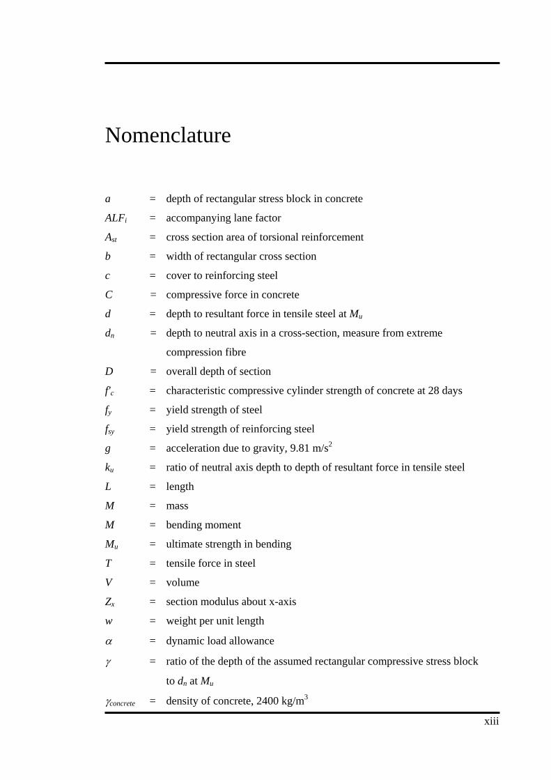
Nomenclature a = depth of rectangular stress block in concrete

ALFi = accompanying lane factor

Ast = cross section area of torsional reinforcement

b = width of rectangular cross section

c = cover to reinforcing steel

C = compressive force in concrete

d = depth to resultant force in tensile steel at Mu

dn = depth to neutral axis in a cross-section, measure from extreme

compression fibre

D = overall depth of section

f'c = characteristic compressive cylinder strength of concrete at 28 days

fy = yield strength of steel

fsy = yield strength of reinforcing steel

g = acceleration due to gravity, 9.81 m/s2

ku = ratio of neutral axis depth to depth of resultant force in tensile steel

L = length

M = mass

M = bending moment

Mu = ultimate strength in bending

T = tensile force in steel

V = volume

Zx = section modulus about x-axis

w = weight per unit length

α = dynamic load allowance

γ = ratio of the depth of the assumed rectangular compressive stress block

to dn at Mu

γconcrete = density of concrete, 2400 kg/m3

xiii

γg = dead load factor

σ = stress

φ = strength reduction factor / capacity factor

xiv

Introduction Chapter 1

Chapter 1

Introduction

1.1 General Background Information

Bridges are a necessity in the transport network. They account for only short sections of

road however they provide a convenient way of joining two inaccessible areas. For this

reason they are used to cross rivers, creeks and other roads such as in the construction of

overpasses on freeways. Bridges can range from small unnoticeable structures to large

impressive man made engineering wonders that are recognised worldwide. Common

examples of these are the Sydney Harbour Bridge in Australia and the Golden Gate

Bridge in the United States of America. These structures are not built this way just to

look impressive. All their components are needed to support the large loads that are

imposed on them.

Versatile and strong materials are needed in the construction of bridges. The most

common of these materials today are reinforced concrete, prestressed concrete and steel.

Reinforced concrete in particular is very popular in the construction of small bridges

since it is very simple to construct a concrete deck that is supported by girders.

Reinforced concrete does not act like typical materials when loaded. Concrete by itself

is very strong in compression, however its tensile strength is very low in comparison. A

standard concrete mix could have a compressive strength of 32 MPa and a tensile

1


strength of only 2 – 3 MPa. To overcome the lack of tensile strength steel bars are added

to the concrete. Therefore in a concrete section the compression forces are taken by the

concrete while the tensile forces are taken by the area of steel that is provided in the

tensile part of the section. This combination of two different materials with very

different properties make the analysis of reinforced concrete more complex than that of

a steel structure. In addition concrete does not have a linear relationship between stress

and strain. Once the concrete is loaded to about 40 % of its compressive strength the

stress-strain relationship becomes increasingly nonlinear by the formation of

microcracks in the interaction between the aggregate and the mortar [1]. Another

property of concrete that makes accurate structural analysis more difficult is that under

biaxial compression, its compressive strength increases. From test results, maximum

gain in compressive strength is obtained when the ratio of the perpendicular stresses

applied is 0.6 [1]. Due to the complex nature of these properties, simplified design

methods were produced that do not accurately predict the true behaviour of concrete

structures.

By applying the finite element method, it is possible to model concrete a lot more

accurately. The finite element method was first developed by Richard Courant and

applied in 1943 in his work on solving a torsion problem [2]. It was not until the 1960’s

and 70’s that it was given the finite element name and further developed to solve a host

of problems, from heat transfer to fluid dynamics and structural analysis [3]. A finite

element model consists of a mesh of elements defined by nodes that describe the

geometrical properties of an object. Section properties are added to describe the

behaviour of the elements. Forces are applied to the nodes, from this the elements

reaction can be determined by parameters such as stresses and displacements. Now with

the increase in the popularity of the finite element method, more accurate models of

material behaviours have been included in finite element software. Concrete can now be

accurately modelled and the analysis can even accounting for the cracking that occurs.

There are various ways of modelling reinforced concrete with the finite element

method. One way of defining reinforced concrete is by superimposing the steel

reinforcement in the generated mesh of plain concrete. This way the concrete is able to

be defined separately from the steel. However in this situation the bond between the

2


steel and concrete is not accounted for. To overcome this tension stiffening is added to

the concrete to account for the steel and concrete bond. The finite element analysis

software ABAQUS [4] is able to effectively model reinforced concrete by the method

described. It is also able to apply a nonlinear analysis to the concrete to derive an

accurate prediction of the stresses and deformation that will occur under loading. This

makes ABAQUS [4] the ideal finite element analysis tool to model the effect that girder

spacing has on a reinforced concrete bridge deck.

1.2 Aims and Objectives

This project aims to use the finite element method to determine the optimum girder

spacing on a composite bridge deck. The bridge under analysis will be comprised of a

reinforced concrete bridge deck supported by steel I-beam girders. A cross section of

the design is shown in Figure 1.1.

Figure 1.1: Cross section of composite bridge deck.

In order to achieve this aim the following objectives have to be met:

1. Research background information of the non-linear behaviour of concrete and

how it is applied in a finite element model.

2. Determine the loading requirements of the bridge from the relevant Australian

Standards.

3


3. Conduct a preliminary design of the bridge.

4. Learn how to effectively use the ABAQUS [4] finite element software.

5. Model the bridge deck using the finite element method.

6. Employ the finite element model to determine the effect of girder spacing on the

deck response.

1.3 Structure of Dissertation

Chapter 1 gives background information on the topic and describes the objectives

needed to achieve the aim of the project.

Chapter 2 gives some background on the use of finite element technique in the analysis

of reinforced concrete structures. It also explains how the finite element method is used

to effectively model the nonlinear behaviour of concrete.

Chapter 3 contains the loading requirements set out by AS 5100.2 [5]. These loads are

then used to determine a preliminary sizing of members for the bridge deck to be used

in the finite element models.

Chapter 4 contains the methodology relating to production of a finite element model.

This starts off with the basics of the ABAQUS [4] software then continues on to the

methodology behind a preliminary model that was produced with the student edition of

ABAQUS [4]. The chapter finishes with the methodology behind the three finite

element models that were used for analysis.

Chapter 5 involves the analysis and discussion of results for the three separate bridges

with different girder spacings. From these results the optimum girder spacing can be

determined.

4


Chapter 6 provides a summary of the analysis undertaken and the conclusions drawn.

This chapter will also give details on future work that can be conducted in relation to the

finite element.

The appendices provide additional material to the project work. These include the

project specification and the input files for the finite element models.

5

Background Research Chapter 2

Chapter 2

Background Research

2.1 Introduction

This chapter will provide information on the properties of concrete and how they are

applied in a finite element model. Reinforced concrete is a composite material

containing a mix of a number of different materials including sand, aggregate, cement

and steel bars. This mix of materials means concrete does not have well defined

constitutive properties like steel. The finite element model then has to apply these

nonlinear properties to produce results that will match the true behaviour of the

reinforced concrete.

2.2 Uniaxial Stress-Strain Relationship

The uniaxial compressive stress-strain relationship for concrete is linear for small stress

values. However once stresses reach approximately 40% of the compressive strength of

the concrete the relationship becomes increasingly nonlinear [1]. This is shown in

Figure 2.1.

6


Figure 2.1: Uniaxial stress-strain relationship for concrete [6].

If the load applied increases, the stress value will reach the peak of the nonlinear curve.

At this point the concrete is at its maximum compressive strength and any additional

loads will cause failure of the bond between the aggregate and the cement paste.

ABAQUS [4] models the compressive stress-strain relationship as elastic and plastic.

Elastic properties are given for the initial linear behaviour. Then specific concrete

properties are used to state the initial yield point and the stress and strain values at

which the concrete fails.

When the concrete has been loaded into the inelastic range and is then unloaded some

elasticity will be lost. While this loss of elasticity is accounted for in the model the

unload/reload response is idealised as a straight line.

The stress-strain relationship in tension is considered linear to its failure point. This is

considered to be 8-10 % of the total compression stress [6]. Once cracks form the

concrete undergoes softening where it is still able to withstand small tensile stresses as

can be seen in Figure 2.1. The effect of this in relation to reinforced concrete will be

explained in the section on tension stiffening.

7


2.3 Combined Stresses

The compressive strength of concrete increases when under biaxial stress. This increase

depends on the magnitude of the lateral compressive stress. Test results have shown the

maximum strength gain is achieved when 12 /σσ is approximately 0.6 [1]. The failure

envelope representing biaxial stress is shown in Figure 2.2. ABAQUS [4] uses this

relationship in its analysis of concrete and also determines a crack detection surface to

account for biaxial compression-tension.

Figure 2.2: Failure envelope for concrete biaxial stress [6].

2.4 Tension Stiffening

When concrete reaches its maximum tensile strength cracks begin to form perpendicular

to the direction the stress has been applied. However the concrete between these cracks

still has the ability to carry stress. Tension stiffening is a term used when the cracked

concrete provides stiffness in conjunction with the reinforcement. It describes the strain

softening behaviour of the concrete after it has cracked and is used to account for the

interaction between the steel reinforcement and the concrete. ABAQUS [4] allows the

8


user to define this softening behaviour for concrete models being analysed. The stress-

strain relationship of a tension stiffening model is shown in Figure 2.3.

Figure 2.3: Tension stiffening model for concrete [6].

2.5 Smeared Crack Approach

ABAQUS [4] uses the smeared crack approach in its analysis of plain concrete. For this

analysis individual cracks are not analysed. Instead when the concrete reaches its failure

surface the stiffness properties of the material are changed in the direction orthogonal to

the crack. This then acts like a crack has formed. As the material properties are only

evaluated at the integration points the alteration of the stiffness properties of the

material effect the region from which these properties are evaluated, therefore smearing

the crack over a whole region. Also there is no permanent strain associated with the

cracking. This allows the cracks to close again if a compressive load is applied.

The smeared crack approach is used in the analysis of reinforced concrete by adding a

layer of steel reinforcement within the concrete. In this situation the steel acts

independently from the concrete. To describe the interaction between the two materials

the tension stiffening model is used.

9


2.6 Finite Element Analysis Accuracy for Concrete

When using finite element analysis on a composite material such as reinforced concrete

there is a chance that the analysis will not produce suitable results. For this reason

research has been undertaken into the accuracy of finite element methods for reinforced

concrete.

There are other analysis techniques such as the discrete method that can be used in place

of the smeared crack approach. It has been stated however that the smeared crack

approach is often the more attractive method to define the cracking of the concrete [7].

The advantage is that there is no need to continuously redefine the element mesh as in

the discrete method, which significantly slows down the analysis.

There have been concerns that the smeared crack approach introduces mesh sensitivity

into the solutions so the finite element results do not converge to a unique result [6].

ABAQUS [4] is able to deal with this to some extent by using Hilleborg’s [8] approach

that can deal with this problem for practical purposes. However the ABAQUS User

Manual [6] states that by having each element contain steel reinforcement, the mesh

sensitivity is reduced. This depends on an adequate amount of tension stiffening being

added to simulate the interaction between the concrete and the steel reinforcement.

Previous research has been conducted into the accuracy of using the finite element

method in the analysis of reinforced concrete bridge decks. Biggs et al. [9] used the

smeared crack approach in comparing experimental test results of a slab to those

produced from the finite element method. Results proved accurate enough for Biggs et

al. [9] to recommend the method to the Virginia Department of Transportation for the

analysis of reinforced concrete bridges. Huria et al. [10] compared their finite element

analysis results with a decommissioned bridge deck that had been tested to failure. The

results obtained from the smeared crack approach closely matched those from the

experimental testing.

10


2.7 Summary

The complex nonlinear properties of concrete such as the uniaxial stress-strain

relationship and the increase in compressive strength under biaxial stress has made it

difficult to predict its true behaviour. Finite element analysis techniques such as the

smeared crack approach have now been developed to closely match these properties.

However as with any theoretical modelling there are always questions about the

accuracy of the results. Research has been conducted comparing experimental testing

results with those produced from the finite element analysis. The conclusions from such

work have shown that concrete can be accurately modelled with the finite element

method.

11

Preliminary Bridge Design Chapter 3

Chapter 3

Preliminary Bridge Design

3.1 Introduction

This project involves the design of a bridge using the finite element software ABAQUS

[4]. The bridge is comprised of a concrete deck supported by longitudinal steel girders.

All bridges in Australia must meet Australian Standards to ensure their safety. In

particular, Part 2 of the Bridge Design Code [5] is important as it states what loads the

bridge will be required to support. Lane and shoulder widths also must meet the

Australian Standards to ensure safe passages of vehicles across the bridge.

Once the loading and overall dimensions of the bridge are accounted for a rough design

is obtained from traditional design methods. This is done for a number of reasons. A

starting point is needed with the finite element model in terms of girder sizes and slab

thicknesses. The author had no previous experience in designing bridges. Therefore the

approximate depth of the concrete slab and the girder sizes are not known. The design

can also be used for a rough comparison with the results from the finite element

analysis. If the finite element analysis produces results that are greatly different from

those calculated in this section then there is a good chance a mistake has been made.

The following sections of this chapter outline the dimensions of the bridge, the loading

requirements and present a preliminary design of member sizes required to meet these

loads.

12


3.2 Bridge Dimensions and Features

A typical cross section of a bridge consisting of steel girders supporting a reinforced

concrete slab is shown in Figure 3.1.

Figure 3.1: Typical cross section of bridge deck.

3.2.1 Bridge Features

The steel I-beam girders run longitudinally between the supports. Sitting on top of these

is the reinforced concrete slab with reinforcement in the top and bottom for negative and

positive bending moments respectively. The concrete slab is attached to the top flange

of the girders with shear studs. These transmit shear loads along the plane of the slab.

Diaphragms run between the girders and are used to provide lateral restraint and

counteract buckling of the girders. Concrete safety barriers are placed on each side for

vehicle crash safety.

3.2.2 Bridge Dimensions

The first item to determine for the bridge is its dimensions. It is assumed that the bridge

runs over a small creek and therefore does not have a great span. The only limit on the

span chosen is the maximum moment that can be supported by a standard I-section. The

13


maximum span of a Welded I-Section produced by One Steel (a producer of structural

sections in Australia) is 18 m. These welded sections range in depth from 700 mm to

1200 mm [11]. To ensure these beams can take the moments applied, the distributed

load that the maximum size section can withstand over an 18 m span is calculated.

Figure 3.2: 1200WB455 cross section.

1200WB455 Section properties:

331025600

280

mmZ

MPaf

x

y

×=

=

Maximum moment girder can support:

kNmMM

ZM x

71682801025600 3

=××=

= σ

Maximum distributed load 18 m long girder can support:

mkNw

w

LMw

wLM

/1771871688

88

2

2

2

=

×=

=

=

14


The result determined the girder could support 177 kN/m, which is over 17 tonne per

metre for the entire length of the girder. Therefore it can be assumed that an 18 m long

girder can easily support the weight of traffic above it as long as the spacing between

girders is adequate. This quick check does not account for buckling. However if

buckling is a problem in the finite element design then extra diaphragms can be added

to counteract the buckling effect.

The width of the bridge depends on the Australian Standards for lane and shoulder

widths. In particular it is dependant on the amount of traffic the bridge will carry. It is

assumed the bridge spans a creek in the country and therefore will not experience high

traffic flows. It is also assumed that there is no need for a pedestrian walkway. Table 9.5

of AS5100.1 [12] states edge clearances from the edge of the traffic lane to the face of

the safety barrier for bridges without walkways. From this table with a traffic volume of

500 – 5000 vehicles per day the edge clearance required is 1000 mm. As for lane

widths the Austroads publication, Rural Road Design [13] states that the desirable lane

width on rural roads should be 3.5 m for traffic volumes of 1000 – 3000 vehicles per

day.

The last item to determine the exact geometric requirements of the bridge is the concrete

barriers placed on either side. A standard barrier was chosen from AS/NZS 3845 Road

Safety Barrier Systems [14]. The 1100 High VCB Road Safety Barrier System chosen

complies with Test Level 3. This is an Australian Standard test level that will restrain all

passenger cars and four wheel drives in the event of an impact. The barrier is shown in

Figure 3.3.

15


Figure 3.3: 1100 High VCB road safety barrier system [14].

Taking into account the values above, the geometric layout of the bridge is shown in the

plan view, Figure 3.4.

Figure 3.4: Plan view of bridge.

3.3 Loading Requirements

To provide a realistic analysis the loading on the bridge must comply with AS 5100.2

[5]. To determine the most adverse effects on the bridge there are a number of different

16


loads that are required to be applied by the Australian Standard. Since the aim of this

dissertation is to find the optimum girder spacing, braking forces will be ignored.

The loads defined by AS 5100.2 [5] that are applied to the bridge are listed below:

- Dead load.

- W80 wheel load.

- A160 axle load.

- M1600 moving traffic load.

- S1600 stationary traffic load.

These loads must have factors applied to determine the design loads for ultimate and

serviceability limit states. These are listed below:

- (γg) dead load factor.

- (α) dynamic load allowance.

- (ALFi) accompanying lane factor.

3.3.1 Load Factors for Dead Load of Structure

Clause 5.2 of AS 5100.2 [5] states the load factors required for the dead load of the

structure. The factors that are relevant to this bridge are listed in Table 3.1.

Table 3.1: Load factors for dead load of structure [5].

Ultimate Limit States Where Dead Load Type Of

Construction Reduces Safety

Increases Safety

Serviceability Limit States

Steel 1.1 0.9 1 Concrete 1.2 0.85 1

17


3.3.2 Dynamic Load Allowance

The dynamic load allowance is a factor accounting for dynamic and vibratory effects of

the bridge under loading conditions. It is in essence the static equivalent of the dynamic

effects of vehicles moving over the bridge with road surface irregularities [5]. It is

applied to the load in question with the following expression:

( ) ionconsideratunder action factor load1 action design ××+= α

The value of the dynamic load allowance for the appropriate loading is shown in Table

3.2.

Table 3.2: Dynamic Load Allowance [5].

Loading Dynamic Load Allowance (α)W80 wheel load 0.4 A160 axle load 0.4 M1600 tri-axle group 0.35 M1600 load 0.3 S1600 load 0

3.3.3 Accompanying Lane Factor

When more than one lane is loaded then the loading applied to additional lanes must be

multiplied by the accompanying lane factors. These are given in Table 3.3.

Table 3.3: Accompanying Lane Factors [5].

Standard Design Lane Number Accompanying Lane Factor (ALFi) 1 lane loaded 1.0 2 lanes loaded 1.0 for first lane; and 0.8 for second lane

18


3.3.4 Load Factors

Clause 6.10 of AS 5100.2 [5] states the load factors required for the ultimate and

serviceability loads on the structure. The factors that are relevant to the bridge being

designed are listed in Table 3.4

Table 3.4: Load factors for design road traffic loads [5].

Limit State Traffic Load Ultimate Serviceability

W80 Wheel Load 1.8 1 A160 Axel Load 1.8 1 M1600 Moving Traffic Load 1.8 1 S1600 Stationary Traffic Load 1.8 1

3.3.5 W80 Wheel Load

This models an individual heavy wheel load and consists of an 80 kN load distributed

over a rectangular contact area 400 mm × 250 mm. It is placed in any position on the

bridge that will give the most adverse effect.

3.3.6 A160 Axle Load

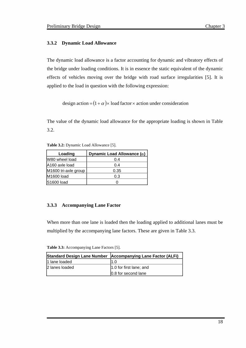
The A160 Axle Load is similar to the W80 wheel load. However it models a single

heavy axle so there are two W80 wheel loads placed at 2000 mm centres. The

application of the load in a standard design lane is shown in Figure 3.5.

19


Figure 3.5: A160 Axle Load [5].

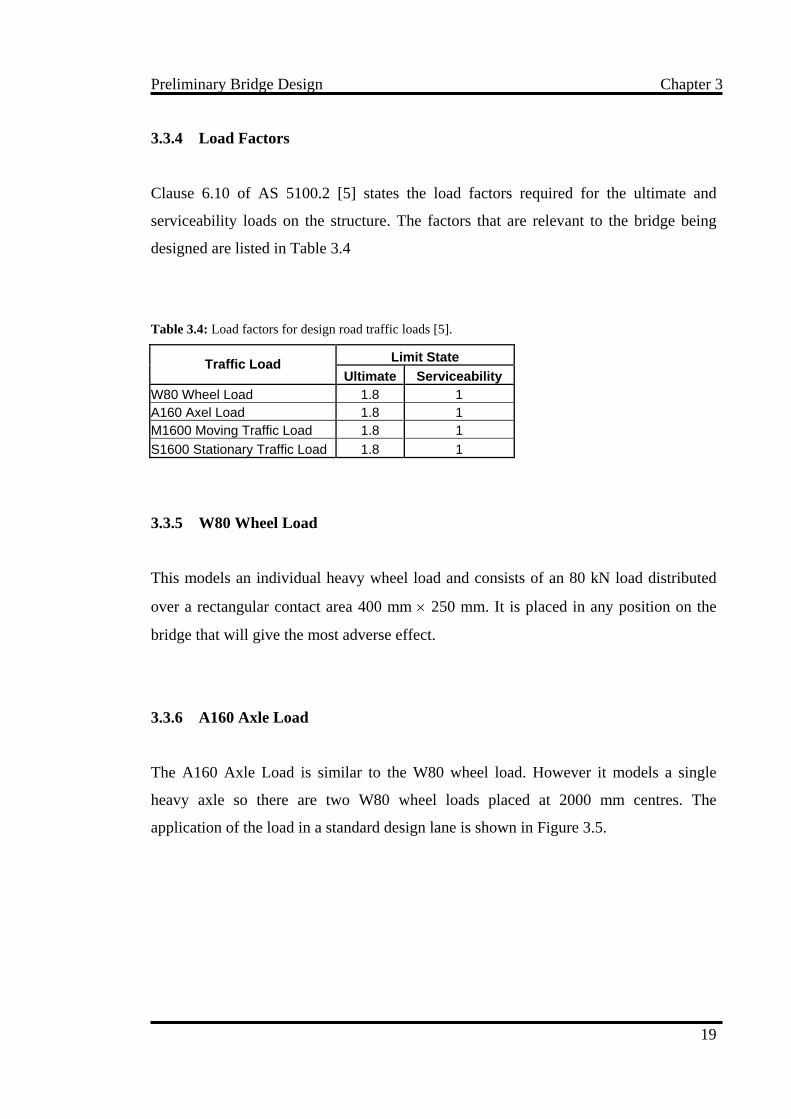
3.3.7 M1600 Moving Traffic Load

This load models a moving stream of traffic across the bridge. The entire load is placed

in a standard 3.2 m wide design lane and continues along the length of the bridge. The

M1600 load consists of a uniformly distributed load placed over the width of the design

lane plus a number of tri-axial groups to represent a constant stream of trucks passing

over the bridge. To achieve the most adverse effects the spacing of the tri-axial groups

may be modified and the distributed load may be continuous or discontinuous for any

length that is necessary. The application and value of the M1600 design loads are

defined in Figure 3.6.

Figure 3.6: M1600 Moving Traffic Load [5].

20


3.3.8 S1600 Stationary Traffic Load

The S1600 stationary traffic load models a stream of stationary traffic on the bridge.

Like the M1600 load it consists of a uniformly distributed load over a standard design

lane plus a series of tri-axial groups. To achieve the most adverse effects the spacing of

the tri-axial groups may be modified and the distributed load may be continuous or

discontinuous for any length that is necessary. The application and value of the S1600

design loads are defined in Figure 3.7.

Figure 3.7: S1600 Stationary Traffic Load [5]

3.4 Preliminary Sizing of Structural Members

The preliminary sizing of members is determined from the worst effect produced by the

design loads defined above. Only a rough size for the structural members is needed.

Bending moments are analysed from the design loads to determine rough section sizes.

To determine the respective bending moments the structural design software Multiframe

[15] is used.

3.4.1 Preliminary Design of the Concrete Slab

The slab has a total width of 9.93 m with a length of 18 m. The dead loads of the slab

are first determined and then combined with the design loads to calculate the maximum

21


bending moments. From these moments the slab thickness and the amount of steel

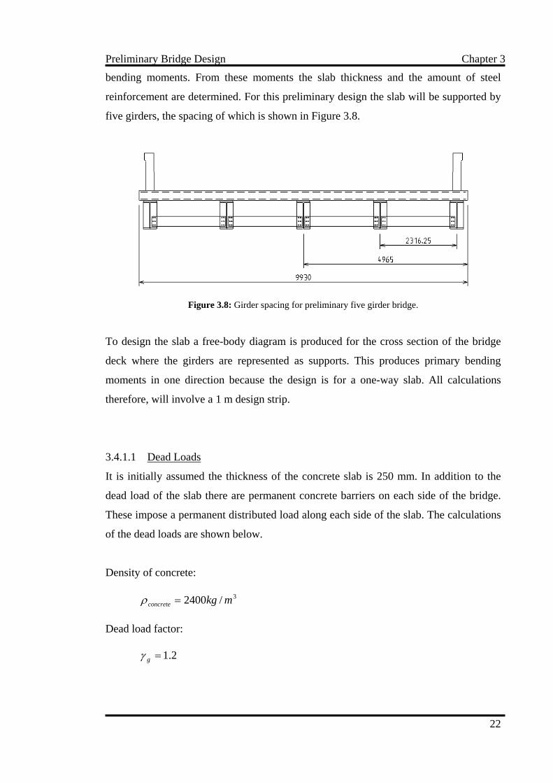
reinforcement are determined. For this preliminary design the slab will be supported by

five girders, the spacing of which is shown in Figure 3.8.

Figure 3.8: Girder spacing for preliminary five girder bridge.

To design the slab a free-body diagram is produced for the cross section of the bridge

deck where the girders are represented as supports. This produces primary bending

moments in one direction because the design is for a one-way slab. All calculations

therefore, will involve a 1 m design strip.

3.4.1.1 Dead Loads

It is initially assumed the thickness of the concrete slab is 250 mm. In addition to the

dead load of the slab there are permanent concrete barriers on each side of the bridge.

These impose a permanent distributed load along each side of the slab. The calculations

of the dead loads are shown below.

Density of concrete:

3/2400 mkgconcrete =ρ

Dead load factor:

2.1=gγ

22


Volume of 1 m wide design strip of slab:

325.025.011 mV =××=

Volume of 1 m length of concrete barrier using dimensions from Figure 3.3:

3286.004.02.02

1.1025.01.1265.0 mV =×+×

−×=

Dead load for 1 m design strip of slab:

mkNWW

gVW concreteg

/06.781.9240025.02.1

=×××=

= ργ

Dead load for 1 m length of concrete barrier:

mkNWW

gVW concreteg

/08.881.92400286.02.1

=×××=

= ργ

3.4.1.2 W80 Wheel Load

The design action for the W80 wheel load is as follows:

( )( )

kN6.201 action Design 808.14.01 action Design

action factor load 1 action Design

=××+=

××+= α

The slab is designed as a cross sectional strip 1 m wide and the design action acts over

an area 0.4 m × 0.25 m. Assuming this area is orientated so the length of 0.4 m runs

across the deck and the length of 0.25 m runs the length of the deck the distributed load

in a 1 m wide design cross section is:

mkNmkN /504

4.06.201

=

The wheel area is spread out over an area 0.4 m × 1 m. This does not produce the exact

bending moment generated from the wheel load however it provides a good

23


approximation. The distributed load is placed on a continuous beam in Multiframe [15]

along with the dead load of the deck to determine the maximum bending moment. The

bending moment produced is shown in Figure 3.9.

Figure 3.9: Bending moment diagram produced from W80 load.

3.4.1.3 A160 Axle Load

The design action for the A160 axle load is two W80 wheel loads placed two meters

apart. The load is imposed so one wheel is placed in the centre of two supports to

generate the maximum bending moment possible. The maximum bending moment from

this load plus the dead load is shown in Figure 3.10.

Figure 3.10: Bending moment diagram produced from A160 axle load in one lane.

The bridge being modelled contains two lanes so the A160 axle load is also imposed on

the second lane. The loads in the second lane are multiplied by the accompanying lane

factor which is 0.8. Therefore each distributed wheel load in the second lane is 403.2

kN/m. The bending moment diagram produced is shown in Figure 3.11.

24


Figure 3.11: Bending moment diagram produced from A160 axle load in both lanes.

3.4.1.4 M1600 Moving Traffic Load

The M1600 load is comprised of 360 kN imposed over six separate areas that represent

the wheel footprints of a truck plus a 6 kN/m distributed load over a 3.2 m lane. The

design action on one wheel area is:

( )( )

kN8.145 action Design 608.135.01 action Design


=××+=

××+= α

The design action of 145.8 kN is distributed over an area 0.4 m × 0.2 m. This area is

orientated so the length of 0.4 m runs across the deck and the length of 0.2 m runs the

length of the deck. The distributed load in a 1 m wide design cross section is:

mkNmkN /5.364

4.08.145

=

The 6 kN/m distributed load is spread over a 3.2 m design lane. All calculations are

based on a 1 m design strip so the distributed load for this design strip is calculated as

follows:

2/875.12.3

/6 mkNm

mkN=

25


The design action is:

( )( )

2/39.4 action Design 875.18.13.01 action Design


mkN=

××+=××+= α

These loads are combined with the dead load of the deck to produce the bending

moment diagram for one lane loaded. This is shown in Figure 3.12.

Figure 3.12: Bending moment diagram produced from M1600 traffic load in one lane.

The second lane is loaded the same as the first however all loads are multiplied by the

accompanying lane factor of 0.8. The bending moment diagram is shown in Figure 3.13.

Figure 3.13: Bending moment diagram produced from M1600 traffic load in both lanes.

3.4.1.5 S1600 Stationary Traffic Load

The S1600 load is defined the same way as the M1600 load with loads over separate

wheel areas and a distributed load over a design lane. In this case there is 240 kN

26


distributed over six wheel areas and 24 kN/m distributed over the 3.2 m design lane.

The design action on one wheel area is:

( )( )

kN72 action Design 408.101 action Design


=××+=

××+= α

The design action of 72 kN is distributed over the same area as the M1600 load and is

orientated the same way. The load is therefore:

mkNm

kN /1804.0

72=

The distributed load over a 1 m design strip:

2/5.72.3

/24 mkNm

mkN=

The design action is therefore:

( )( )

2/5.13 action Design 5.78.101 action Design


mkN=

××+=××+= α

These loads applied to one lane plus the dead load of the deck gave the following

bending moment diagram, Figure 3.14.

Figure 3.14: Bending moment diagram produced from S1600 traffic load in one lane.

27


Again the second land is loaded the same as the first and all loads multiplied by the

accompanying lane factor of 0.8. Results of this are shown in Figure 3.15.

Figure 3.15: Bending moment diagram produced from S1600 traffic load in both lanes.

The maximum moments from the analysis are tabulated in Table 3.5. The W80 wheel

load produced the greatest positive moment of 72.7 kNm. The greatest negative moment

is 85.7 kNm. This is produced from the A160 axle load when only one lane is loaded.

Table 3.5: Maximum moments produced from loading combinations on deck.

Loading Positive Moment (kNm) Negative Moment (kNm)

W80 72.7 40.4 A160 One Lane 56.2 85.7 A160 Two Lanes 55.9 80.8 M1600 One Lane 40.0 65.5 M1600 Two Lanes 42.1 61.8 S1600 One Lane 24.7 40.5 S1600 Two Lanes 24.7 38.4

It is noted that the weight of the concrete barriers are not added into the calculations for

the moments. This is because the barriers run directly on top of the outside girders and

therefore do not impose any bending loads on the deck.

3.4.1.6 Concrete Slab Sizing

In this section a rough design of the concrete slab is undertaken. It sole purpose is to

give approximate dimensions of the concrete slab to be used in the model, such as the

amount of steel reinforcement and the depth of the slab. Therefore this design is based

solely on the stresses imposed by the moments calculated in the previous sections.

28


The first area considered in the design is the durability requirements. It was assumed the

bridge is in a location in South East Queensland and is within 50 km of the coastline.

Therefore from Table 4.3 in AS 5100.5 [16] the exposure classification is B1 and from

Table 4.5 the minimum characteristic strength is 32 MPa. Abrasion requirements are

required to be met in accordance with AS 5100.5 [16]. The minimum compressive

strength for abrasion for pneumatic-tyred traffic heavier than 3 tonne gross mass is 32

MPa. From this it has been decided to use 40 MPa concrete. This was done because the

bridge deck is a major structural element therefore concrete stronger than the minimum

required can only improve the design.

With the strength of the concrete decided the cover required for the steel reinforcement

is determined. Standard compaction and formwork is used for a situation like this, as the

slab would be poured on site. Therefore from Table 4.10.3(A) in AS 5100.5 [16] the

nominal cover to the reinforcement is 40 mm.

With durability requirements accounted for the thickness of the slab and reinforcement

is determined. The rectangular stress block approach is used to determine the ultimate

strength in bending of the slab. Figure 3.16 shows a diagram of the rectangular stress

block approach. This states the maximum strain in the extreme compression fibre of

concrete is 0.003.

Figure 3.16: Rectangular stress block at ultimate strength [16].

29


The value of ku must be equal to or less than 0.4 to ensure the section has a ductile

failure. In this situation the steel yields before the concrete in compression fails,

therefore if the structure is overloaded it will not catastrophically collapse.

Reinforcement is run in both the top and bottom of the slab because there are positive

and negative moments. However as this is a basic design the section sizes will be

determined by only accounting for the steel in tension. The slab thickness is initially

assumed to be 250 mm deep with 12 mm reinforcement bars placed at 100 centres.

Predefined values:

MPafMPafmmD

mmc mm crs

smm dia bar

sy

c

50040'

25040

100 spacing reo12size reo

====

==

Calculating γ which is ratio of the depth of the assumed rectangular stress block to kud

when the structure is under bending or bending and compression:

( )( )

766.02840007.085.028'007.085.0

=−−=−−=

γγγ cf

Assuming the reinforcement bar diameter is 12 mm the effective depth of the cross-

section is:

mmdd

diabarcDd

204640250

. 21

=−−=

−−=

30


The reinforcement used is 12 mm bars run at 100 mm centres, therefore the total area of

steel over a 1 m design strip is equal to 1130 mm2. The ultimate moment capacity of the

section is now determined.

Compression force in concrete:

NdCdC

dbfC

n

n

nç

26044766.040100085.0

8.0

=××××=

= γ

Tension force in steel:

kNTT

AfT stsy

5651130500

=×=

=

Applying equilibrium conditions where C=T to determine the neutral axis depth:

mmdd

TC

n

n

69.2156500026044

==

=

Determining the depth of the stress block:

mmaa

da n

62.16766.069.21

=×=

= γ

31


Calculating the ultimate moment capacity of the section by applying a lever arm from

the centre of the steel to the centre of the rectangular stress block:

kNmM

M

adTM

6.110262.16204565

2

=

⎟⎠⎞

⎜⎝⎛ −×=

⎟⎠⎞

⎜⎝⎛ −=

Checking ku to ensure the section is ductile:

1.0204

69.21

=

=

=

u

u

nu

k

k

dd

k

The value of ku is less than 0.4 therefore the section is considered ductile.

From AS 5100.5 Table 2.2 [16] the capacity reduction factor is 0.8 for bending without

axial tension or compression where ku ≤ 0.4. Appling this to the maximum moment

capacity of the section:

kNmMM

u

u

48.88 6.1108.0

=×=

φφ

The design capacity of the section is 88.48 kNm. This value is greater than the design

moment of 85.7 kNm therefore adopt a 250 mm thick slab with 12 mm reinforcement

bars at 100 mm centres. For simplicity of the design it is assumed that this

reinforcement runs in the top and bottom of the slab in both directions.

32


3.4.2 Preliminary Design of Steel Girders

In the preliminary model the slab is supported by five girders spaced at 2316.25 mm

centres. The girders are I-beam sections with a span of 18 m. The dead load imposed on

the girders is first determined and then combined with the design loads to determine the

maximum bending moments. The size of the I-beam required is calculated from the

bending moments.

The free-body diagram for the girders consists of a simply supported span between two

supports. It is assumed that the centre girders will support a 2.316 m width of slab. This

is used for all calculations to give the greatest bending moments.

3.4.2.1 Dead Loads

The dead loads imposed on the girders are from the concrete slab and the self weight of

the girder. Each one-meter length along the girder supports a slab area of 2.316 m × 1

m. The calculations for the dead load due to the slab and the girders are shown below.

Volume of slab supported by 1 m length of girder:

3579.025.01316.2

mVV

LBDV

=

××==

The dead load from the concrete slab on the girder is therefore:

mkNWW

gVW concreteg

/36.1681.92400579.02.1

=×××=

= ργ

Assume a 900WB282 I-beam is used. This has a depth of 900 mm and a mass of 282

kg/m. The dead load of this beam per metre is:

33


mkNW

W

mgW g

/32.381.92822.1

=××=

= γ

Therefore the total dead load for every metre length of girder is:

mkNWW

/68.1932.336.16

=+=

3.4.2.2 W80 Wheel Load

The design action for the W80 wheel load was determined previously for the loading on

the deck. It was calculated as 201.6 kN over an area 0.25 m × 0.4 m. As the girders run

perpendicular to the deck this load will be orientated so it is distributed over a length of

0.25 m on the girder. The distributed load is:

mkNmkN /4.806

25.06.201

=

This load is placed in the centre of an 18 m span of a simply supported beam to generate

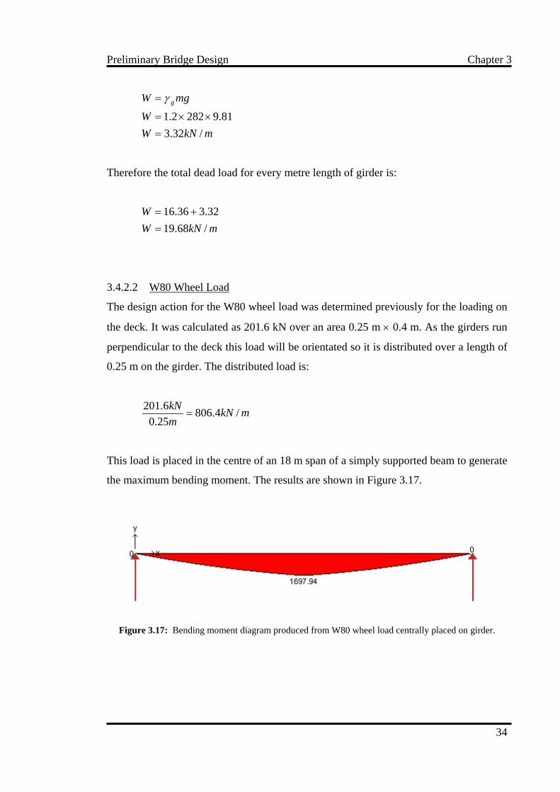
the maximum bending moment. The results are shown in Figure 3.17.

Figure 3.17: Bending moment diagram produced from W80 wheel load centrally placed on girder.

34


3.4.2.3 A160 Axle Load

The distance between girders is 2.316 m and the total distance between the outside of

the wheel footprints representing the A160 load is 2.4 m. It is therefore assumed that the

greatest loading on one single girder will be when one of these wheels is directly above

the girder and placed in the centre. This gives the same bending moment as the W80

wheel load shown in Figure 3.17.

3.4.2.4 M1600 Moving Traffic Load

Like the A160 axle load the distance between the outside of the two wheel footprints is

2.4 m. However there is also a distributed load that acts over a 3.2 m width. It is

assumed that the maximum load on the girder will occur when one row of wheels is

directly above it. It is also assumed that half of the M1600 distributed load will act on

the girder. The spacing of the wheel footprints is in accordance with Figure 3.6 to

produce the greatest bending moment. Due to the wheel footprint sizes each wheel load

is distributed over a 0.2 m length along the girder. The design action for the M1600 load

was calculated in section 3.4.1.4. Applying this over a 0.2 m length gives:

mkNmkN /729

2.08.145

=

Half of the distributed M1600 load will act on the girder, this is calculated below:

mkN /02.76.139.4 =×

There is only need to design for one lane, as the loading from the second lane will act

on a different girder. Also due to the accompanying lane factor the loading is less,

producing a smaller bending moment. The diagram of the resulting bending moment

from the M1600 load is shown in Figure 3.18.

35


Figure 3.18: Bending moment diagram produced from M1600 traffic load placed on girder.

3.4.2.5 S1600 Stationary Traffic Load

The S1600 stationary traffic load is placed on a girder in the same way as the M1600

load. The design actions for the A1600 load were determined in section 3.4.1.5. The

distributed loads for the girder are calculated below.

The wheel load distributed over a 0.2 m length of girder:

mkNm

kN /3602.0

72=

Half of the S1600 load distributed on the girder:

mkN /6.216.15.13 =×

Again like the M1600 load there is no need to calculate both lanes loaded at once

because a different girder will support the second lane. Applying the dead loads and the

live loads in the same way as the M1600 load gives the bending moment diagram

shown in Figure 3.19.

Figure 3.19: Bending moment diagram produced from S1600 traffic load placed on girder.

36


The maximum moments from the analysis are tabulated in Table 3.6. The M1600

moving traffic load produced the greatest bending moment of 3794 kNm.

Table 3.6: Maximum moments produced from loading combinations on girder.

Loading Positive Moment (kNm)W80 1698 A160 1698 M1600 3794 S1600 3011

3.4.2.6 Girder Sizing

In this section the girder size is determined from the bending moments produced above.

It sole purpose is to give an approximate size of the girders to be used in the finite

element model.

From HRSSP [11] the yield stress in a welded I-beam section is around 280 MPa for the

flanges and 300 MPa for the web. The exact yield stresses depend on the size of the

section. To be on the cautious side it is assumed the yield stress through the entire

section is 280 MPa. The elastic section modulus required to withstand this bending

moment is calculated below:

3310135502803794

mmZMPakNmZ

MZ

x

x

x

×=

=

=σ

The welded beam with a section modulus that closest matches the answer above is a

1000WB322. As the section modulus of this beam is larger at 14600 × 103 mm3 the

maximum stress in the girder is less than the yield stress. Therefore adopt a

1000WB322 girder to be used in the finite element model.

37


3.5 Summary

This chapter defined the loading requirements needed for a road bridge built in

Australia. It then applied these requirements in the preliminary sizing of bridge

members to be used in the finite element analysis. A 250 mm thick concrete slab

comprising of 40 MPa concrete was chosen. From this the required cover to

reinforcement was 40 mm. To withstand the ultimate bending loads the reinforcement

was 12 mm bars spaced at 100 centres in the top and bottom of the slab in both

directions. Five girders were chosen to support the concrete deck. From the loads

applied the girder size required to meet the maximum bending moment was a

1000WB322 I-beam.

38

Model Methodology Chapter 4

Chapter 4

Model Methodology

4.1 Introduction

Three bridge deck configurations, each with a different number of girders ranging from

three to five are analysed using the finite element software ABAQUS [4]. Initially, the

ABAQUS [4] student version, with a limitation of 1000 nodes, is used since only

limited access is available to the full version at the CESRC (Computational Engineering

and Science Research Centre) at USQ. This is to help the author to familiarise himself

with the software and modelisation techniques before attempting to produce models on

the full version with an increased number of nodes.

4.2 ABAQUS Software

ABAQUS [4] is one of the world leaders in advanced Finite Element Analysis. It

provides complete and powerful solutions for routine and sophisticated linear and

nonlinear engineering problems. It contains different analyses modules such as

ABAQUS Standard for general nonlinear solid mechanics, ABAQUS Explicit for

dynamic problems, and ABAQUS Aqua for fluid mechanics, CAE and Viewer for pre-

and post-processing.

ABAQUS CAE, which stands for ABAQUS Computer Aided Engineering, is a

graphical interface, which allows the user to input all the model data, run the analysis,

39


and view the results. During the analysis, a basic ASCII file with the extension “.inp” is

produced. The file contains all the model information and can be simply opened with a

text editor. This file is very useful since information regarding certain aspects of the

model that cannot be defined within CAE can be added to the input file. The modified

input file can then be submitted as an analysis job using the command line within the

operating system shell.

During an analysis, ABAQUS [4] generates a large number of output files, among them

are the output database file “.odb”, the data file “.dat”, and the message file “.msg”. The

first here is a binary file that provides the information required by the Viewer to provide

the graphical representation of the results. The data file is a text file that contains

information about the model and its history definition generated by the analysis. It also

contains an output of results that have been requested, and any error or warning

messages that were detected. All diagnostic and informative messages about the

progress of the solution are contained within the message file. All errors and warnings

are detailed in the message file with the results of this tabulated at the end of the

message file.

If the analysis of a model is based around an input file then the Viewer section of

ABAQUS [4] comes into use. It reads the output database file and provides a graphical

representation of all requested results. This can be seen by a contour diagram drawn

over the part, a displacement diagram of the part or an x-y plot of the requested output.

4.3 Layout of an ABAQUS Model

To effectively produce a model with ABAQUS [4], specific information must be given

so the finite element analysis can take place. There are a number of steps to producing a

finite element model and these all have to be correctly accounted for before the model

will run and valid answers can be produced. An ABAQUS [4] model consists of two

parts: model geometry, and model history.

40


4.3.1 Model geometry

The model geometry contains different parts of the model that are assembled together,

the material properties of these parts and in some situations how they are tied together.

A mesh of nodes and elements defines each part with each node given a location in a

Cartesian coordinate system and each element being defined by a number of these

nodes. During this process the type of element is also stated. All the information

regarding the part is contained within a part option. A section option is used within the

part option to give the section properties of the particular part. This is used to define the

dimensions of the elements that constitute the part, the material used and any other

parameters or data that are deemed necessary.

Once all the parts have been defined they can be assembled as a number of part

instances. For example there is more than one girder in the bridge but they are all

identical so only a mesh of one girder is needed. When it comes to assembling the

bridge the first girder is defined as Girder – Instance-1 and the second as Girder –

Instance-2. This continues in the same fashion until all the girders are defined in the

assembly. Even though there is one deck it still has to be defined as an instance as the

visualisation section of ABAQUS [4] runs off part instances. Each instance is

positioned in the global coordinates by a translation in the x, y and z directions and by a

rotation defined by an axis of rotation and an angle.

Material definitions provide the model with the information needed for the analysis of

the material behaviour. Steel is an elastic material so the inputs for the model will be

Young’s modulus and Poisson’s ratio. However as ABAQUS [4] can undertake a

nonlinear analysis the yield stress of the steel can also be input under the material

properties. This means that the plastic strain of the material can be measured if the

stresses are high enough. ABAQUS [4] has a wide range material definitions that allow

modelling of most materials. In terms of this project they have a number of plastic

models for concrete with one suited to the analysis of reinforced concrete. This is the

smeared crack approach.

41


Contact and interaction is used to join parts together and define friction properties

between them. This is often defined as part of the model geometry but sometimes

interaction properties can be applied as model history. Nodes, elements and surfaces are

used to define particular contact and interaction restraints. For example various amounts

of friction can be applied between two surfaces or two nodes can be tied together so

their global displacements and rotations are the same.

4.3.2 Model history

The model history contains the steps in the analysis, loads, boundary conditions and

output requests.

The analysis of an ABAQUS [4] model is run as a series of steps. There is always a

minimum of two steps. The first step is automatically built in to the analysis and is used

to apply the boundary conditions. Following steps define the loading conditions and

outputs required. If contact has been defined as part of the model history then a separate

step is required before the load step to define this contact.

Numerous loading situations can be modelled with ABAQUS [4], from point loads

applied on nodes to distributed loads on elements or surfaces.

A boundary condition is produced by restraining various degrees of freedom at a node.

The number of degrees of freedom for a particular node will depend on the element

used. Although in structural situations such as this each node will nearly always have

six degrees of freedom, three displacement and three rotation. The boundary conditions

fix certain parts of the model so there will be support reactions to counteract the loads

applied to the structure.

When it comes to producing results ABAQUS [4] automatically has a standard list of

outputs if none are defined. These contain most of the properties needed for a general

structural analysis such as stress, strain and displacement. If other outputs are required

42


these can be defined. These results can be output to the output database file for use in

the Viewer or written to the data file as a list of results.

4.4 The Input File

The entire finite element model is defined in the input file. All information displayed in

the input file is given in terms of keywords. Each keyword starts with an asterisk and is

then often followed by a parameter. For example the keyword *element is used to

define the elements of a part. It is then followed by the required parameter type to

define what type of element it will be. Keywords are often followed by data lines which

give additional information required. In the example given above for the *element

keyword the data lines contain the element number and the nodes that make up the

element. All information that relates to a particular keyword is referred to as an option.

Therefore all the information given above is described as an element option.

Often when defining options, the elements or nodes that the option acts upon must be

previously stated. This is done by grouping nodes or elements into sets by using either

the *nset or *elset option respectively. This ends up being the bulk of the input file as

once a node set or element set is established it only requires an option that may be one

or two lines to impose the contact, boundary conditions and other details that are

required.

4.5 Initial Modelling – Student Edition

4.5.1 Background

Modelling was initially started by using ABAQUS CAE, as it has a graphical user

interface and makes it much easier to produce a working finite element mesh. Once the

mesh is produced, all the relevant data is added to the input file using a text editor.

43


4.5.2 Preliminary Model Details

Due to the node limitation of the student version, initially a model of a bridge deck with

only two girders and three diaphragms running between the girders is produced. This

model is not realistic, and is only produced as a learning process on how to effectively

use ABAQUS [4].

4.5.2.1 Elements Used

The deck and the girders are modelled with three dimensional shell elements while the

diaphragms are modelled using truss elements. Shell elements are used when one

dimension, the thickness, is significantly less than the other two dimensions.

Conventional shell elements have six degrees of freedom, three being displacement

degrees with the other three defining rotation.

S4R elements are used to discretise the deck. This is a conventional four node,

quadrilateral, stress/displacement shell element with reduced integration and a large

strain formulation. It is a rectangular shaped element with a node at each corner. The

properties of the section are calculated by using the shell section option. This uses

numerical integration through the thickness of the shell and is suited to solving

nonlinear problems, in this case the analysis of a reinforced concrete deck. In this

option the thickness of the shell and the number of integration points are defined. The

ABAQUS [4] documentation recommends at least nine integration points when

analysing concrete.

The girders also use S4R elements. There are beam elements in ABAQUS [4] however

these are only defined as a line. The shape of the cross section is then given in the

section definition for the part. Therefore when it comes to analyse the part an accurate

stress distribution cannot be obtained through the section. This is why the I-beam

girders are produced with shell elements. The user is then able to see the shape of the

girder and how the stresses and displacements vary between the flanges and web of the

girder.

44


To model the steel reinforcement in the concrete, rebar elements are used. These are

elements within ABAQUS [4] specifically designed to model steel reinforcement. They

are added as layers to existing elements in a smeared layer where the thickness is equal

to the area of reinforcement bar divided by the reinforcement bar spacing. To define this

in ABAQUS [4] the rebar layer option is used. For this option the following information

must be stated: the name of the reinforcement layer; the cross sectional area and spacing

of the reinforcement; the location in the thickness direction measured from the midpoint

of the shell and the angle of the reinforcement in relation to the x-direction.

The diaphragms that run between the girders are modelled with truss elements. These

are long slender elements that can only transmit axial forces. They cannot transfer

moments. Truss elements were chosen because the diaphragms sole purpose is to

transmit axial forces to prevent buckling of the girders. The T3D2 truss element was

used in the model. This is a two-node 3-D truss element. Section details for the element

are defined by the solid section parameter. The only inputs needed are the cross

sectional area of the section and the name of the material it is made from.

4.5.2.2 Connections

Once all the parts have been assembled and the section properties for each have been

defined the next step is to provide connections between these separate parts. This allows

forces and moments to transfer between parts just as they would in the real world.

When a bridge such as this is constructed the concrete deck is tied to the girders by the

way of shear connectors. These are studs than protrude from the girders and are cast into

the concrete. They are spaced along the length of the girder at constant intervals and can

either be multiple rows of studs or just a single line down the centre. This situation is

modelled using the *contact pair option with the tied parameter. To apply this

interaction, the first step is to define the top surface of each girder and the bottom

surface of the deck plus list the *surface interaction and *surface behaviour options.

Once this is done the *contact pair option ties the two surfaces together when they

come in contact with each other. A hard pressure overclosure relationship is chosen for

45


the surface behaviour. This does not allow the slave nodes to penetrate into the master

surface. The top of the girders are defined as the slave surface and the bottom of the

deck is defined as the master surface. ABAQUS [4] attempts to find the closest point on

the master surface that matches up with a node on the slave surface. This is where the

master surfaces normal passes through the node on the slave surface and the interaction

is then discretised between a point on the master surface and a slave node. An adjust

parameter is also used for this option. This adjusts the position of the nodes on the slave

surface at the start of the simulation so they precisely contact the master surface. Even

though this way of modelling shear connectors is not exactly the same as the real

situation it was determined that it would be an accurate representation as the vertical

loads being transferred between the deck and the girders would be the same.

The diaphragms have to be attached to the girders. As the diaphragms are modelled with

truss elements pinned restraints are chosen. This is done by attaching the node at the end

of the diaphragm to a node on the girder. The *equation option could be used in this

situation as it is designed to define linear multi-point restraints. The restraint requires a

linear combination of nodal variables to be equal to zero. In this situation both nodes

must move together so the three displacement degrees of freedom for the two nodes

must be tied together. This is defined by the equation shown where u is the nodal

variable at node D or G and 3 is the degree of freedom in question.

GD uu 33 =

Rearranging so the variables are equal to zero gives:

033 =− GD uu

The properties of the equation are defined in the input file as two data lines. The first

line states the number of terms in the equation, in this case there are two. The second

line states the first node in question, the degree of freedom for that node and the

coefficient for that node which is one. This is repeated for the second node with the

coefficient being negative one so the equation equals zero. Only one degree of freedom

46


can be restrained per equation so three equations are used for each constraint to tie all

three degrees of freedom

4.5.2.3 Boundary Conditions

The boundary conditions are set up to represent a simply supported structure. One end

of the structure is be pinned while the opposite end is a pinned/sliding restraint. This is

the closest way to model how the bridge would act when sitting on bearing pads without

actually modelling them. Bearing pads have very little shear support so they will take

any deformation in the long direction of the bridge.

The *boundary option is used to apply the boundary conditions. Data required for this

option is that the nodes be given boundary conditions, and the degrees of freedom to be

restrained. The nodes chosen are on the bottom side of the girders at each end as this is

where the supports are. At one end the nodes are restrained for the three displacement

directions. At the opposite end the nodes are only restrained in two directions. The

direction the nodes are not supported in is the direction that runs the length of the

bridge. This gives a sliding restraint for the simply supported condition.

4.5.2.4 Materials

The model contains only two main materials, steel and concrete. The *material option

is used to define these. Within this option other options are used to define the material

properties.

For steel the elastic properties are defined with Young’s modulus as 200 GPa and

Poisson’s Ratio as 0.3. Plastic properties are not used at this stage because the main aim

is to produce a working finite element model. The density of the steel is listed as 7850

kg/m2 [11] so it can be used to determine the loading from the self-weight of the bridge.

The concrete is defined with elastic and specific concrete properties to define its

behaviour outside the elastic range. These values are taken from Gilbert and Warner

[17]. The ABAQUS Example Problems Manual [6] used these values in the analysis of

47


a concrete slab and some of their assumed values are also been used in this analysis, as

they are not available from Gilbert and Warner [17]. The properties outside the elastic

range are listed as yield stress with respect to plastic strain. The first stress-strain point

is used to list the initial yield point of the concrete so the plastic strain value must be

equal to zero. This yield stress is assumed in the ABAQUS Example Problems Manual

[6] and this value of 20.68 MPa is used in the model. The next stress strain point is the

failure ratio for the concrete, this is taken from Gilbert and Warner [17] and listed as

37.92 MPa with an assumed plastic strain at failure of 1.5 × 10-3. Elastic properties are

again from Gilbert and Warner [17] with a Young’s Modulus of 28.6 GPa and Poisson’s

Ratio of 0.15. Finally for self weight loads the density of the concrete is listed as 2400

kg/m2 [16].

4.5.2.5 Analysis Steps

For the bridge being modelled a general static analysis step is chosen. This effectively

models the nonlinear behaviour of both the concrete and the steel. The *static option is

used to define this and because it is a nonlinear analysis details have to be given on the

time step. The default values that ABAQUS [4] recommends are used. These are an

initial time increment of 1, a step period of 1, 1 × 10-5 for the minimum time increment

allowed and 1 for the maximum time increment allowed.

The loads for this basic model are just the self-weight of the girders and deck. These are

defined by a gravity load. The option *dload is used with the inputs being the elements

for each of the girders and the deck, the parameter grav to define the loading as being

gravity, the acceleration due to gravity which is 9.81 m/s and the direction in which it

acts. In the model this is the negative z-direction. ABAQUS [4] uses the density of each

material that is defined in the material property definitions and the acceleration due to

gravity and then multiplies these by the volume of each element making up the part.

This gives the distributed loading that results from the self-weight of the structure.

The *output option is used to state the results requested from the simulation. The

default outputs are chosen for the model by the preselect parameter. No specific results

are required as this model is used as a learning experience. There are two different types

48


of output, field output and history output. Field outputs are the results that are written at

fairly low frequencies from a large portion of the entire model. These include variables

such as stress and strain. History outputs are results that are written at fairly high

frequencies from a small portion of the model. These include variables such as the

displacement of a single node. An x-y plot of history results can also be produced. This

can be used to show the displacement of a node over the time of the simulation.

4.6 Three, Four and Five Girder Models

After the initial trial model had been produced with the student edition, and an

understanding of how to create a model of the bridge-deck was obtained, the next step is

to move onto the full version of ABAQUS [4]. New models with more degrees of

freedom are created. These are a three, four and five girder deck and from this the

optimum girder spacing will be obtained. The input file for each model can be found in

Appendix B.

4.6.1 Member Sizes

The member sizes used in the three separate models remained the same even though the

number of girders would vary. This is done to limit the variables encountered when it

came to determining an optimum girder spacing. Sizes used are similar to those

determined in Chapter 3 with the Preliminary Bridge Design.

The girder size used is the largest 1000 welded beam produced by OneSteel. This is an

I-beam 1024 mm deep with a flange width of 400 mm and a weight of 322 kg/m [11].

The maximum available length of this beam is 18 m and is what is used in all models. A

cross section of this beam is shown in Figure 4.1.

49


Figure 4.1: 1000 WB 322 I-Beam

The concrete slab used in all three models is a 250 mm deep slab with 10 mm

reinforcement bars at 100 mm spacing. This spacing is run in both directions in the top

and bottom of the slab. The reinforcement is reduced from the 12 mm bars designed in

Chapter 3 so the nonlinear response of the deck would be more pronounced. Cover is 40

mm top and bottom to adhere to Australian Standards. Details of this are explained in

Chapter 3.

As there is no preliminary design for the diaphragms the sizes for these are assumed

values. However Biggs et al. [9] in their analysis of a similar bridge used channel

sections 380 mm deep. For the analysis 300 × 32 mm plates are chosen. These are

attached to web stiffeners at the centre and ends of the girders.

4.6.2 Elements

The elements that are used have already been determined in the preliminary model, the

difference here being that all the elements are smaller so more accurate results will be

obtained. S4R shell elements are used for the deck and girders and B31 beam elements

for the diaphragms. Specific rebar elements are added to the deck to model the

reinforcement.

50


The deck is meshed with a total of 2940 elements. This is produced as a rectangular

mesh with 70 elements spanning the 18 m length of the deck and 42 elements spanning

the 9.93 m width. The element size is therefore 0.257 m × 0.236 m respectively. When

meshing the girders the element length is kept the same as the deck with 70 elements

spanning the length of the girder on the both the flange and web of the beam. Both the

flanges and the web of the beam have 8 elements spanning their width and depth

respectively. Each of the web stiffeners has elements sizes so that they matched the web

and flange elements of the girders. A total of 1872 elements are used in the girders.

Unlike the girders and the deck the number of elements change for the diaphragms

depending on the model. This is due to their different lengths caused by the varying

girder spacing in the models. The diaphragms in the five girder bridge contains six

elements while ten elements are used for the four girder model and eighteen elements

are used for the three girder bridge deck. The diaphragms are modelled using B31 beam

elements that are able to take bending moments and axial loads. These are chosen since

the diaphragms are fixed to the girders with more than one bolt. Such a connection

creates full restraint and allows bending moments to be transferred from the girders to

the diaphragms.

The beam element B31 is a two node linear beam with the standard six degrees of

freedom. It is defined as a one-dimensional element in three-dimensional space. The

section is defined with the *beam section option. This accounts for the nonlinear

response of the material. ABAQUS [4] has predefined sections available as parameters,

and a rectangular section is chosen to model the plates. The data needed for this option

is the dimensions of the plate and the direction of the plates n1 vector. In the case of the

model this is in the z-direction.

4.6.3 Connections

The deck is tied to the girders using the *tie option. Contact surfaces of the girders and

deck need to be pre-defined for this option. The only parameters that are to be stated is

the type of tie, which is a surface to surface interaction, and to set the adjust parameter

51


to yes. This initially moves all tied nodes on the slave surface onto the master surface

without causing any strain.

A MPC (Multi Point Constraint) is used to attach the diaphragms to the girders. This is

defined with the *mpc option. The tie parameter is used to restrain all six degrees of

freedom for the node on the diaphragm to the node on the girder. This enabled moments

to be transferred between the two parts as they would under real conditions.

4.6.4 Boundary Conditions

The boundary conditions for the bridge deck are applied to model a simply supported

condition. One end of the girders is pinned in all three directions and at the opposite end

a pinned/sliding arrangement is defined. The length of the deck would subsequently be

free to change when loaded.

The supporting area of the boundary conditions is changed between models as each

contains a different number of girders. If the supporting area is kept the same between

models then the reaction forces at the boundary conditions in the three girder model

would be a lot higher than that in the five girder model. For this reason the five and four

girder models have boundary conditions spanning over two rows of elements at the end

of each girder. This is increased to three rows of elements for the three girder model.

4.6.5 Materials

The material definition for concrete is defined with a number of options. The density is

specified as 2400 kg/m3 [16] so the self-weight of the structure can be applied as a load.

The elastic properties are defined with Young’s Modulus of 28.6 GPa and Poisson’s

Ratio of 0.15. The specific concrete properties are defined with an initial yield stress of

20.68 MPa* and a failure stress of 37.92 MPa at a plastic strain of 1.5 × 10-3*. Tension

stiffening properties are used in concrete model to account for the stress taken between

the cracks that have formed. It is defined as the fraction of remaining stress to stress at

52


cracking and the absolute value of the direct strain minus the direct strain at cracking. In

the models, for zero remaining stress the value of direct strain is listed between 0.001 to

0.01. The tension stiffening value is purely theoretical and is changed between models

to ensure the solution will converge to a result. All of these values are taken from

Gilbert and Warner [17] or where marked with an asterisk taken from the ABAQUS

Example Problems Manual [6].

Three separate material properties for steel with different yield stresses are defined in

the model. The girders consist of two types of steel according to HRSSP [11]. The web

of the girders is 300 MPa steel while the flanges are 280 MPa steel. The reinforcement

modelled is standard N class bars with a yield stress of 500 MPa. These yield points are

listed in the input file by using the *plastic option and stating the yield stress of the

steel. The elastic properties are the same for all steel and listed as with Young’s

modulus as 200 GPa and Poisson’s Ratio as 0.3. A density of 7850 kg/m2 [11] is listed

so the self-weight of the structure can be applied as a load.

4.6.6 Analysis Steps

A general static analysis step is chosen for the analysis. This will effectively model the

nonlinear behaviour of the materials. The default values that ABAQUS [4] recommends

are used for the time step. This is an initial time increment of 1, a step period of 1,

1 × 10-5 for the minimum time increment allowed and 1 for the maximum time

increment allowed.

Loading from AS 5100.2 [5] is applied to model the design loads. The exact loads and

their positions on the bridge are defined in Chapter 2. All the loads defined in AS

5100.2 [5] are either footprints of wheel loads or a distributed load over the deck. These

are all applied by the *dsload option in ABAQUS [4]. This is a loading option to define

a distributed load over an element or surface. The elements that accounted for the wheel

footprints are gathered into an element set and then defined as a surface. The elements

that account for the distributed load over the deck are defined as a separate surface. The

element sizes in the model meant that the wheel footprints are not exactly the same area

53


as those defined in the code. However the overall load applied is still exactly the same.

Once the elements constituting the surfaces are selected the type of distributed load is

set as a pressure and the magnitude of this is defined. This same procedure is used for

the self-weight of the concrete barriers that are applied to the deck. The loads due to the

self-weight of the parts are defined by gravity loading.

The default outputs are used for the analysis. However a few other output requests are

included to obtain all the results that are required. The stress for the reinforcement in the

concrete is requested to be written to the data file. This gives a table of the stress and

force in the reinforcement at each element in the bridge deck plus maximum and

minimum values. The *el print option is used where the elements requested for output

need to be defined and the output variables for stress and force are stated. The stress in

the diaphragms is written to the data file in the same way. ABAQUS [4] is also able to

state if cracks have formed in the concrete and in what direction. This is done by using

the same *el print option as above and by stating the crack output variable. The results

for this are in tabular form that show what elements have cracked, which surface they

are cracked on and the direction of the normal to each crack. A history output request is

used so a plot of a node displacement can be produced for the time period of the

simulation. This will show if the deck is loaded enough for the concrete to be effected

by nonlinear behaviour. It is defined in the model by the *node output option where the

node in question was listed plus the direction in which the displacement will be

measured.

4.7 Conclusion

A number of finite element models were produced of the bridge deck for various

loading combinations and girder spacings. The results from the analysis of these models

will be presented in the next chapter and from this the optimum girder spacing will be

determined.

54

Results Chapter 5

Chapter 5

Results

5.1 Introduction

This chapter presents and explains the results obtained from the finite element analysis.

Three bridge-decks were modelled with ABAQUS [4]. These ranged from a three girder

bridge deck to a five girder bridge deck. Each has the same girder size, 1000WB322 I-

beams and the same slab. This is a 250 mm thick 37.92 MPa concrete slab with 10 mm

reinforcement bars top and bottom running in both directions.

All bridges were modelled using nonlinear material behaviour laws. This is particularly

important for the slab, as cracking occurs at small tensile stresses in the concrete

causing a shift in the neutral axis of the section. ABAQUS [4] is able to analyse the

nonlinear behaviour and give results of stress, strain and deflection. Stress shows if the

parts can withstand the loads applied. If the stress is greater than the failure or yield

stress of the concrete or steel respectively then it is known that the part has failed.

Plastic strain is important in the analysis of the girders, as it shows if any of the steel is

overloaded and yielded. Displacement results from the analysis are important as they

are used to check serviceability requirements. The midspan deflection of the deck must

not exceed the limit defined by the AS 5100.2 [5].

55

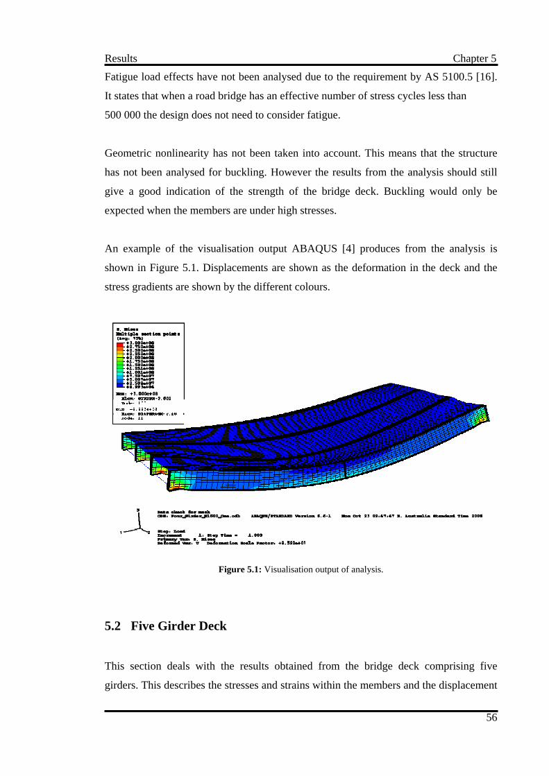
Results Chapter 5

Fatigue load effects have not been analysed due to the requirement by AS 5100.5 [16].

It states that when a road bridge has an effective number of stress cycles less than

500 000 the design does not need to consider fatigue.

Geometric nonlinearity has not been taken into account. This means that the structure

has not been analysed for buckling. However the results from the analysis should still

give a good indication of the strength of the bridge deck. Buckling would only be

expected when the members are under high stresses.

An example of the visualisation output ABAQUS [4] produces from the analysis is

shown in Figure 5.1. Displacements are shown as the deformation in the deck and the

stress gradients are shown by the different colours.

Figure 5.1: Visualisation output of analysis.

5.2 Five Girder Deck

This section deals with the results obtained from the bridge deck comprising five

girders. This describes the stresses and strains within the members and the displacement

56

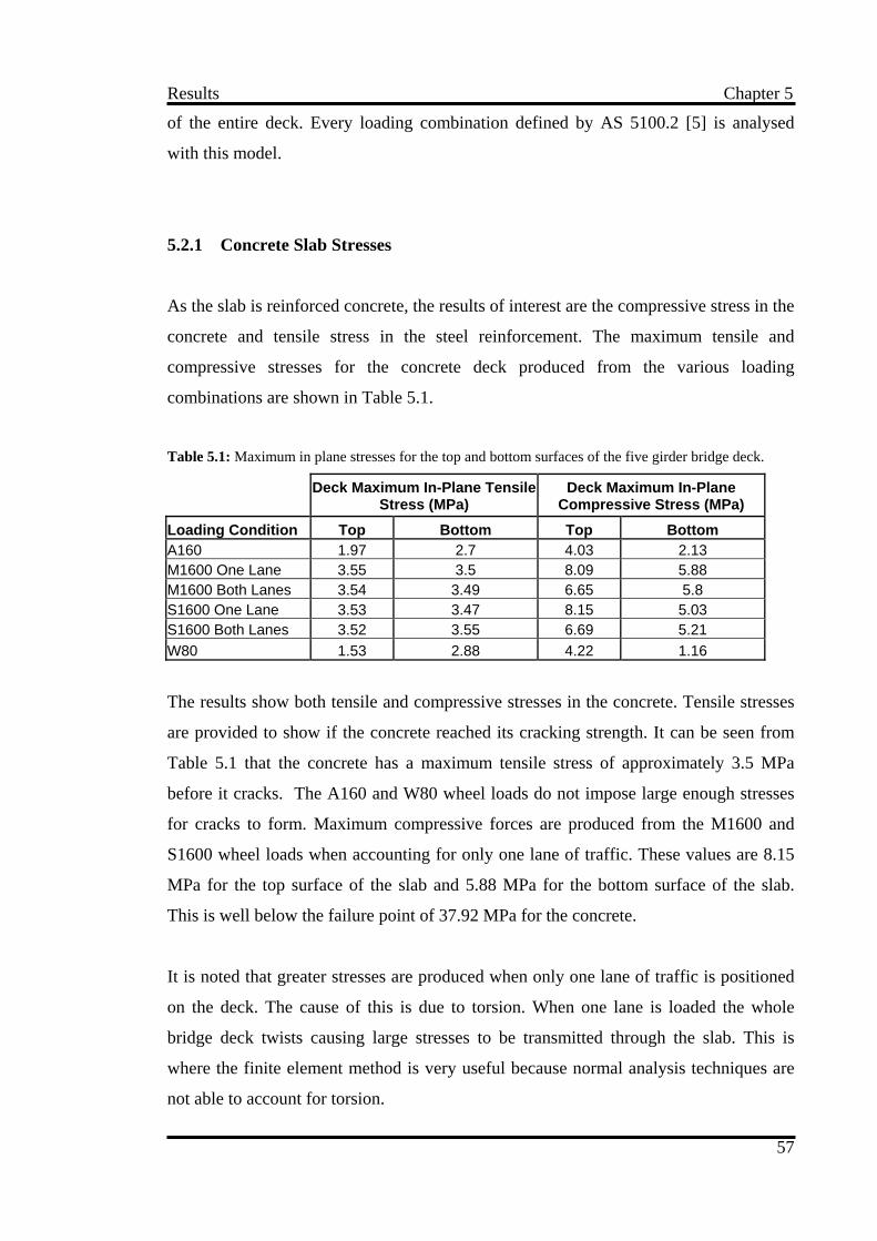
Results Chapter 5

of the entire deck. Every loading combination defined by AS 5100.2 [5] is analysed

with this model.

5.2.1 Concrete Slab Stresses

As the slab is reinforced concrete, the results of interest are the compressive stress in the

concrete and tensile stress in the steel reinforcement. The maximum tensile and

compressive stresses for the concrete deck produced from the various loading

combinations are shown in Table 5.1.

Table 5.1: Maximum in plane stresses for the top and bottom surfaces of the five girder bridge deck.

Deck Maximum In-Plane Tensile

Stress (MPa) Deck Maximum In-Plane

Compressive Stress (MPa) Loading Condition Top Bottom Top Bottom A160 1.97 2.7 4.03 2.13 M1600 One Lane 3.55 3.5 8.09 5.88 M1600 Both Lanes 3.54 3.49 6.65 5.8 S1600 One Lane 3.53 3.47 8.15 5.03 S1600 Both Lanes 3.52 3.55 6.69 5.21 W80 1.53 2.88 4.22 1.16

The results show both tensile and compressive stresses in the concrete. Tensile stresses

are provided to show if the concrete reached its cracking strength. It can be seen from

Table 5.1 that the concrete has a maximum tensile stress of approximately 3.5 MPa

before it cracks. The A160 and W80 wheel loads do not impose large enough stresses

for cracks to form. Maximum compressive forces are produced from the M1600 and

S1600 wheel loads when accounting for only one lane of traffic. These values are 8.15

MPa for the top surface of the slab and 5.88 MPa for the bottom surface of the slab.

This is well below the failure point of 37.92 MPa for the concrete.

It is noted that greater stresses are produced when only one lane of traffic is positioned

on the deck. The cause of this is due to torsion. When one lane is loaded the whole

bridge deck twists causing large stresses to be transmitted through the slab. This is

where the finite element method is very useful because normal analysis techniques are

not able to account for torsion.

57

Results Chapter 5

Figure 5.2: Maximum in-plane compressive stress for the top surface of the slab supporting the M1600

single lane traffic load.

The stresses vary considerably across the slab with high localised stress points in areas

that would not normally be considered. Figure 5.2 shows the maximum in-plane

compressive stress for the top slab surface with a M1600 single lane traffic load. This

output from ABAQUS [4] gives the greatest negative stress at each element, and where

there is no negative stress it gives the smallest positive stress.

The areas under compressive stress are clearly visible by blue, green, yellow and brown

areas with blue representing the areas of highest compressive stress. The highest

stresses are in the areas expected, directly where the loading is applied. However this

image only shows the maximum negative stress values for each element so it does not

give a complete picture on the stresses in the top face of the slab. Figure 5.3 shows the

maximum tensile stresses recorded at each element in the top surface of the slab.

58

Results Chapter 5

Figure 5.3: Maximum in-plane tensile stress for the top surface of the slab supporting the M1600 single

lane traffic load.

The red, yellow and orange areas in Figure 5.3 are all in tension. Comparing Figure 5.2

to 5.3 shows how some elements are in compression and tension. In Figure 5.2 the

majority of the slab was seen to be in compression, however in Figure 5.3 there is a

tension zone highlighted by yellow and orange running the length of the slab. In this

area the concrete is in compression in the x-direction (length direction of deck) and

tension in the y-direction (width direction of deck). A continuous support condition is

provided for the slab by the girders. This allows negative bending moments to be

produced over the girders that result in tensile stresses in the top face of the slab.

However the girders are affected by a positive bending moment that results in

compressive stresses in the concrete. This produces an element that is in both tension

and compression on the same face.

Figure 5.3 also has a small area high in tension at the midspan point along the bottom

edge of the slab. This is caused by the girders web stiffener. The stiffener prevents the

inboard flange of the outer girder from deflecting and as a consequence a stress

concentration results in that area.

59

Results Chapter 5

The areas above each end of the girders show high tensile stresses in Figures 5.2 and

5.3. These high stress areas can also be found on the bottom surface of the slab as large

compressive stresses. Figure 5.4 gives the best representation of these stresses, which

are highlighted by the blue areas at each end of the slab.

Figure 5.4: Maximum in-plane tensile stress for the bottom surface of the slab supporting the M1600


The high stresses in the slab at the end of the girders are due to the support conditions

and the stiffness of the girders. The boundary conditions were applied over a series of

elements at the end of each girder and restrained movement in the vertical direction.

This causes a sharp bend in the girder at the edge of each support and because the

girders are stiffer than the slab stress concentrations formed.

The tensile forces in the steel reinforcement must be assessed to ensure they are within

the yield limit of the steel. The stress carried by each rebar element was written as a

table to the output data file. The maximum tensile and compressive stress for all loading

combinations with the five girder bridge deck is displayed in Table 5.2.

60

Results Chapter 5

Table 5.2: Maximum reinforcement stress for the five girder bridge deck.

Maximum Stress in Steel

Reinforcement (MPa) Loading Condition Tension Compression A160 15.23 21.67 M1600 One Lane 30.77 45.82 M1600 Both Lanes 42.19 36.9 S1600 One Lane 28.15 46.17 S1600 Both Lanes 42.3 37.06 W80 16.77 19.48

Stresses in the steel reinforcement are very low for the five girder bridge deck with a

maximum tensile value of only 42.19 MPa. This is much smaller than the steel yield

stress of 500 MPa. The maximum tensile stresses are due to the M1600 and S1600 loads

when two lanes of traffic are imposed on the deck. The reinforcement containing high

tensile stresses is located on the top surface of the slab above the supports for the

girders. The same high stress areas previously discussed for the concrete slab.

The maximum compressive stresses in the steel are also shown in Table 5.2 because a

majority of the values are higher than the tensile stresses. The maximum compressive

stresses are located where the slab was completely in compression through its cross

section or where tensile stresses are very small in comparison to compressive stresses.

An example of where this has occurred is above the web stiffener on the outside girder.

Normally this would not produce the highest reinforcement stresses in the model but in

this case the slab is well over designed. Small stress concentrations are therefore giving

the maximum recorded values.

Results provided by the analysis show that the reinforced concrete slab for the five

girder bridge deck can withstand all loading requirements defined by AS 5100.2 [5].

61

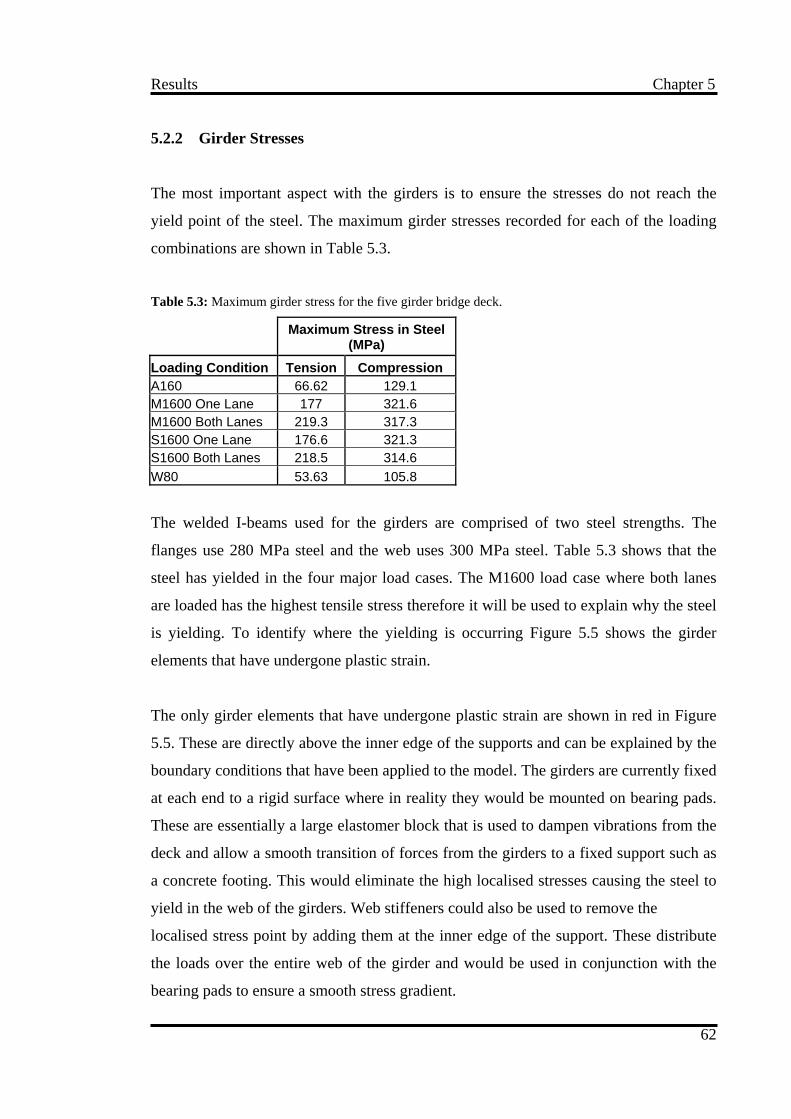
Results Chapter 5

5.2.2 Girder Stresses

The most important aspect with the girders is to ensure the stresses do not reach the

yield point of the steel. The maximum girder stresses recorded for each of the loading

combinations are shown in Table 5.3.

Table 5.3: Maximum girder stress for the five girder bridge deck.


(MPa) Loading Condition Tension Compression A160 66.62 129.1 M1600 One Lane 177 321.6 M1600 Both Lanes 219.3 317.3 S1600 One Lane 176.6 321.3 S1600 Both Lanes 218.5 314.6 W80 53.63 105.8

The welded I-beams used for the girders are comprised of two steel strengths. The

flanges use 280 MPa steel and the web uses 300 MPa steel. Table 5.3 shows that the

steel has yielded in the four major load cases. The M1600 load case where both lanes

are loaded has the highest tensile stress therefore it will be used to explain why the steel

is yielding. To identify where the yielding is occurring Figure 5.5 shows the girder

elements that have undergone plastic strain.

The only girder elements that have undergone plastic strain are shown in red in Figure

5.5. These are directly above the inner edge of the supports and can be explained by the

boundary conditions that have been applied to the model. The girders are currently fixed

at each end to a rigid surface where in reality they would be mounted on bearing pads.

These are essentially a large elastomer block that is used to dampen vibrations from the

deck and allow a smooth transition of forces from the girders to a fixed support such as

a concrete footing. This would eliminate the high localised stresses causing the steel to

yield in the web of the girders. Web stiffeners could also be used to remove the

localised stress point by adding them at the inner edge of the support. These distribute

the loads over the entire web of the girder and would be used in conjunction with the

bearing pads to ensure a smooth stress gradient.

62

Results Chapter 5

Figure 5.5: Plastic strain in girders for two lanes of the M1600 load on the five girder bridge deck.

If the stress concentrations at the supports are not accounted for the girders can easily

take the bending loads applied. The maximum stress recorded on the bottom flange of a

girder for the five girder bridge deck is 125 MPa. The compressive stress on the top

flange is only 36 MPa. The differences in stresses is due to the concrete deck is acting in

conjunction with top flange of the girder to share the compressive forces.

Ignoring the stresses at the supports, the results provided by the analysis show that the

steel girders for the five girder bridge deck can withstand all loading requirements

defined by AS 5100.2 [5].

5.2.3 Diaphragm Stresses

The stresses in the diaphragms have to be checked for yielding. If high compressive

stresses are found in the diaphragms then they should be checked for buckling, as

nonlinear geometry was not specified in this analysis. The diaphragm stresses recorded

for each loading combination is shown in Table 5.4.

63

Results Chapter 5

Table 5.4: Maximum and minimum stress values for diaphragms in five girder bridge deck.

Stress in Diaphragms

(MPa) Loading Condition Maximum Minimum A160 10.29 0.193 M1600 One Lane 23.51 -0.821 M1600 Both Lanes 22.32 0.606 S1600 One Lane 23.84 -0.853 S1600 Both Lanes 22.71 0.732 W80 8.5 0.384

The results for the loading combinations show the diaphragms are all in tension. The

smallest stress values recorded are in compression, however this was because of the

connection applied between the diaphragms and girders. It is a completely fixed

connection so the diaphragms are able to bend producing positive and negative stresses.

The diaphragms at the midspan of the deck always produced the highest stresses. At

each end of the deck the diaphragms did very little work as the girders were restrained

by both the boundary conditions and by the concrete deck. The maximum stress

recorded is 23.84 MPa under the S1600 traffic load. Although all of the loading

conditions representing traffic produced similar results with less than 2 MPa difference.

Results provided by the analysis show that the diaphragms for the five girder bridge

deck can withstand all loading requirements defined by AS 5100.2 [5].

5.2.4 Deck Displacements

In order to satisfy requirements by AS 5100.2 [5] the deflection must not exceed 1/600

of the span under serviceability conditions. For bridge design this is the same as

ultimate load conditions. The girders are 18 m long however the span of the bridge is

16.97 m because the supports on each end of the girder run the length of two elements

equal to 0.514 m. The deflection limit for the bridge is:

mm3.28600

97.16=

64

Results Chapter 5

The deflections produced from the finite element analysis for each loading condition is

shown in Table 5.5.

Table 5.5: Maximum deflection values for all loading combinations on the five girder bridge deck.

Loading Condition Displacement (mm) A160 8.28 M1600 One Lane 17.56 M1600 Both Lanes 16.63 S1600 One Lane 17.82 S1600 Both Lanes 16.9 W80 6.81

The maximum deflection recorded is 17.82 mm for one lane of the S1600 stationary

traffic load. This is only 0.26 mm different from one lane of the M1600 moving traffic

load. All values are less than the limit of 28.3 mm. The results show greater

displacement when only one lane is loaded. As with the deck stress analysis this is due

to torsion being applied to the bridge deck.

A history output was requested of the node under maximum deflection. A plot of this is


Figure 5.6: Displacement plot of node under maximum deflection for a single lane S1600 load.

65

Results Chapter 5

In Figure 5.6 the time scale represents the load applied. At time 1 the load has not been

applied and at time 2 the load is fully applied. The displacement of this node is linear

which shows that the stresses within the concrete are not great enough to cause

nonlinear behaviour.

Results provided by the analysis show that the five girder bridge deck is within

deflection limits for all loading requirements defined by AS 5100.2[5].

5.3 Four Girder Deck

The four girder bridge deck is analysed in the same way as the five girder bridge deck.

However the amount of load combinations have been reduced. The A160 axle load and

the W80 wheel load are not analysed because the results from these loads were never a

limiting factor in the design.


The maximum compressive stresses produced from the various loading combinations

are shown in Table 5.6.

Table 5.6: Maximum in-plane stress for the top and bottom surface of the four girder bridge deck.

Deck Maximum In-Plane

Compressive Stress (MPa) Loading Condition Top Bottom M1600 One Lane 8.41 9.84 M1600 Both Lanes 9.84 10.71 S1600 One Lane 8.66 7.79 S1600 Both Lanes 9.9 8.78

The maximum compressive stresses produced in the slab are only slightly greater than

those produced from the five girder deck. However this time the maximum stresses

66

Results Chapter 5

occur when both lanes are loaded with the M1600 load producing the maximum

compressive stress of 10.71 MPa. Figure 5.7 shows the maximum in-plane compressive

stress for the top slab surface with two lanes of an M1600 moving traffic load.



Blue, green, yellow and orange all show areas that are in compression. The maximum

compressive load is spread out around the centre of the slab in blue. From this it can be

seen that the web stiffeners on the outer girders are again causing stress concentrations.

The red areas show that above each girder high tensile stresses are being produced.

The largest compressive stress is produced on the bottom surface of the slab. In Figure

5.8 it can be seen that this is located at the end of the girders above the supports. These

are the areas in dark blue.

67

Results Chapter 5

Figure 5.8: Maximum in-plane compressive stress for the bottom surface of the slab supporting the

M1600 single lane traffic load.

The steel reinforcement stresses in the slab were only slightly greater than those

produced in the five girder deck. The maximum tensile and compressive stresses for the

reinforcement in the four girder bridge deck is displayed in Table 5.7.

Table 5.7: Maximum reinforcement stress for the four girder bridge deck.

Stress in Steel

Reinforcement (MPa) Loading Condition Tension Compression M1600 One Lane 59.23 45.81 M1600 Both Lanes 54.48 51.09 S1600 One Lane 45.13 47.57 S1600 Both Lanes 41.94 53.2

The single lane M1600 load produced the highest tensile stress in the reinforcement of

59.23 MPa. This was on the far right edge of the deck centred between two girders. The

wheel load placed at that location was not the sole cause of the maximum stress value.

As the edge of the deck is loaded it is unable to transfer the stress in both directions.

68

Results Chapter 5

This results with the reinforcement in the y-direction having to respond by taking more

stress than it would if it was located at the centre of the deck.

The compressive stresses in the reinforcement are not as pronounced as they were in the

five girder model. The increased span between the girders produced larger bending

moments, which in turn increased the tensile stresses in the reinforcement. With the four

girder model these stresses are becoming larger than the compressive stresses caused by

small stress concentrations.

Results provided by the analysis show that the reinforced concrete deck for the four

girder bridge deck can withstand the loading requirements defined by AS 5100.2 [5].


The maximum girder stresses recorded for each loading combination are shown in Table

5.8.

Table 5.8: Maximum girder stress for the four girder bridge deck.


(MPa) Loading Condition Tension Compression M1600 One Lane 181.7 328.9 M1600 Both Lanes 255.5 340.2 S1600 One Lane 195.3 331.5 S1600 Both Lanes 272.1 341.1

The results produced from the analysis show that the steel is yielding with all

compression values larger than the yield stress of 300 MPa. This is due to the same

cause pointed out with the five girder model. The higher tensile stresses are due to the

support conditions in the model not allowing a smooth transition of stress to the

supports. The high tensile stress points are located on the web stiffeners at each end of

the girders.

69

Results Chapter 5

The maximum stresses at the midspan of the girder give a true indication of the strength

of the section. The maximum tensile stress recorded in the bottom flange is 146 MPa

and the maximum compressive stress recorded in the top flange is 42 MPa. These are

well below the 280 MPa yield stress of the girder.

Ignoring the stresses at the supports results provided by the analysis show that the steel

girders for the four girder bridge deck can withstand the loading requirements defined

by AS 5100.2 [5].


The diaphragm stresses recorded for the various loading combinations is shown in Table

5.9.

Table 5.9: Maximum and minimum stress values for diaphragms in four girder bridge deck.

Stress in Steel (MPa)

Loading Condition Maximum Minimum M1600 One Lane 24.99 -0.143 M1600 Both Lanes 36.21 1.44 S1600 One Lane 26.55 -0.880 S1600 Both Lanes 38.01 1.29

All the diaphragms are primarily in tension with very small compression values due to

the small bending that is occurring. The maximum stress value of 38.01 MPa is still

small in comparison to the yield stress of the steel. Even though the diaphragms are

plates there is still no chance of them buckling as they are all in tension.

Results provided by the analysis show that the diaphragms for the four girder bridge

deck can withstand the loading requirements defined by AS 5100.2[5].

70

Results Chapter 5


The maximum deflection limit for the bridge deck required by AS 5100.2 [5] is 28.3

mm. The results recorded for the different loading combinations on the four girder

bridge deck are shown in Table 5.10.

Table 5.10: Maximum deflection values for loading combinations on the four girder bridge deck.

Loading Condition Displacement (mm) M1600 One Lane 20.95 M1600 Both Lanes 30.41 S1600 One Lane 21.72 S1600 Both Lanes 31.61

From the results obtained it can be seen that when both lanes of the bridge are loaded

the deflection recorded exceeds the maximum limit. This was expected in a situation

such as this because serviceability requirements are often the defining factor in

structural design situations.

A deflection plot of the node under maximum displacement is shown in Figure 5.9.

Figure 5.9: Displacement plot of node under maximum deflection for a dual lane M1600 load.

71

Results Chapter 5

The plot of displacement with respect to the load applied produced a linear relationship.

This shows that the concrete is not loaded enough for the nonlinear stress-strain

relationship to come into effect.

Results provided by the analysis show that the four girder bridge deck is not within

deflection requirements defined by AS 5100.2 [5]. Even though the stresses in the deck

and girders are well within their limits the four girder model is not an acceptable design.

5.4 Three Girder Deck

Only the four major load combinations are applied to the three girder bridge deck.

These are the M1600 and S1600 loads with one and two lanes of traffic. It is already

known that the deflection with this model will be greater than that of the four girder

bridge deck and therefore be an unacceptable design. However the three girder bridge

deck is analysed to see if the concrete will show nonlinear behaviour due to the

increased stresses.


The compressive stresses produced from the various loading combinations are shown in

Table 5.11.

Table 5.11: Maximum in-plane stress for the top and bottom surface of the three girder bridge deck.

Maximum In-Plane

Compressive Stress (MPa) Loading Condition Top Bottom M1600 One Lane 20.77 22.49 M1600 Both Lanes 19.8 24.88 S1600 One Lane 17.42 20.89 S1600 Both Lanes 16.38 20.45

72

Results Chapter 5

The stresses are now significantly larger than those produced with the four and five

girder decks with a maximum recorded stress of 24.88 MPa. This is still less than the

failure stress of 37.92 MPa. The maximum compressive stresses were located on the

bottom surface of the slab at each end of the centre girder. These are seen in Figure 5.10

by the dark blue areas. These resulted from the negative bending moments produced in

the girder and slab at this location.

Figure 5.10: Maximum in-plane compressive stress for the bottom surface of the slab supporting the

M1600 dual lane traffic load.

The green areas at the midpoint of the top and bottom of edges of Figure 5.10 show that

the web stiffeners are still causing significant stress concentrations. The compressive

stresses are approximately 10 MPa higher in these areas than the surrounding slab.

The compressive forces in the top concrete face are highest at each end of the slab,

centred between the girders. The blue areas in Figure 5.11 show these compressive

forces. As was explained in the four girder model the loads have been applied so some

of the wheel loads from the M1600 and S1600 traffic loads are placed at the very end of

the slab. The stresses are higher in these areas because the loads cannot be transferred in

both the x and y-directions.

73

Results Chapter 5


dual lane traffic load.

With the increased stress recorded in the concrete the tensile stress in the reinforcement

would have to increase. This was the case with the results shown in Table 5.12.

Table 5.12: Maximum reinforcement stress for the three girder bridge deck.

Stress in Steel

Reinforcement (MPa) Loading Condition Tension Compression M1600 One Lane 251.6 104.1 M1600 Both Lanes 211.3 107.9 S1600 One Lane 186.7 89.7 S1600 Both Lanes 169.8 86.4

The stresses recorded are much greater than those in the four and five girder models

with a maximum recorded stress 251.6 MPa for the M1600 single lane load. This is

located on the bottom layer of reinforcement midway between two girders at the end of

the deck. This is the same area where the maximum compressive forces in the concrete

are found. Even though the stress values are much higher than previous models they are

still well under the failure stress of the steel at 500 MPa. It is also noted that the

74

Results Chapter 5

difference between the ultimate compression and tension stresses are now much greater

as the bending moments across the deck are significantly greater than those produced in

the other models.

Results provided by the analysis show that the reinforced concrete slab for the three

girder bridge deck can withstand the loading requirements defined by AS 5100.2 [5].


The maximum girder stresses recorded for each loading combination are shown in Table

5.13.

Table 5.13: Maximum girder stress for the three girder bridge-deck.


(MPa) Loading Condition Tension Compression M1600 One Lane 282.2 338.8 M1600 Both Lanes 337.8 345.3 S1600 One Lane 281.7 339.1 S1600 Both Lanes 336.7 345.0

From Table 5.13 it is seen that the stresses in both tension and compression are

exceeding the yield point of the steel. However these yield points are again at the

supports. Figure 5.12 shows the contour diagram of plastic strain for the centre girder

with both lanes under the M1600 load.

The contour plot clearly shows that the only areas that have yielded are the areas above

the supports. It has been stated previously that the high stresses in these areas would be

reduced if the bearing pads were modelled in the analysis. The steel is still within its

limits at the midpoint of the girder where a true indication of its strength can be

assessed. The maximum stress value recorded at this point in the bottom flange is 215

MPa and the stress at the top flange is 156 MPa. Both are within the yield limits for the

steel.

75

Results Chapter 5

Figure 5.12: Plastic strain of the centre girder in the three girder bridge deck under M1600 dual lane

traffic load.

Ignoring the stresses at the supports results provided by the analysis show that the steel

girders for the three girder bridge deck can withstand the loading requirements defined

by AS 5100.2 [5].


The diaphragm stresses recorded for the various loading combination are shown in

Table 5.14.

Table 5.14: Maximum and minimum stress values for diaphragms in three girder bridge deck.


(MPa)

Loading Condition Maximum Minimum M1600 One Lane 35.37 -4.31 M1600 Both Lanes 47.18 3.27 S1600 One Lane 36.95 -3.87 S1600 Both Lanes 46.11 1.01

76

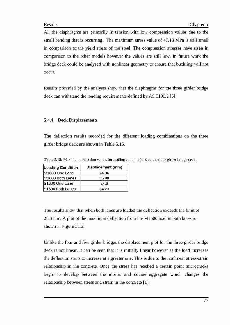
Results Chapter 5

All the diaphragms are primarily in tension with low compression values due to the

small bending that is occurring. The maximum stress value of 47.18 MPa is still small

in comparison to the yield stress of the steel. The compression stresses have risen in

comparison to the other models however the values are still low. In future work the

bridge deck could be analysed with nonlinear geometry to ensure that buckling will not

occur.

Results provided by the analysis show that the diaphragms for the three girder bridge

deck can withstand the loading requirements defined by AS 5100.2 [5].


The deflection results recorded for the different loading combinations on the three

girder bridge deck are shown in Table 5.15.

Table 5.15: Maximum deflection values for loading combinations on the three girder bridge deck.

Loading Condition Displacement (mm) M1600 One Lane 24.36 M1600 Both Lanes 35.88 S1600 One Lane 24.9 S1600 Both Lanes 34.23

The results show that when both lanes are loaded the deflection exceeds the limit of

28.3 mm. A plot of the maximum deflection from the M1600 load in both lanes is


Unlike the four and five girder bridges the displacement plot for the three girder bridge

deck is not linear. It can be seen that it is initially linear however as the load increases

the deflection starts to increase at a greater rate. This is due to the nonlinear stress-strain

relationship in the concrete. Once the stress has reached a certain point microcracks

begin to develop between the mortar and course aggregate which changes the

relationship between stress and strain in the concrete [1].

77

Results Chapter 5

Figure 5.13: Displacement plot of node under maximum deflection for a dual lane M1600 load.

Results provided by the analysis show that the three girder bridge deck is not within

deflection requirements defined by AS 5100.2 [5]. Even though the stresses in the slab

and girders are within their limits the three girder model is not an acceptable design.

5.5 Optimum Girder Spacing

Results from the finite element analyses of three different girder spacings have been

analysed. It has been determined that the four girder model would provide an optimum

spacing for a two lane bridge to meet Australian Standards.

All stresses in the members of the four girder bridge deck were well within the yield and

failure limits. In fact they are low enough that the thickness of the concrete slab and the

amount of steel reinforcement could be reduced while still meeting strength

requirements. However the bridge deck did not meet the deflection requirements

defined by AS 5100.2 [5]. Deflection values were only slightly larger than the limit

therefore this was considered a minor problem because a welded I-beam one size larger

could be used. This would allow the bridge deck to meet serviceability requirements.

78

Results Chapter 5

The three girder bridge deck also meet strength parameters and failed with deflection

requirements. It has been dismissed as being the optimum girder spacing for a number

of reasons. The slab has shown some nonlinear behaviour that is the result of excessive

cracking. The bridge could last for a few months or longer however the cracks would

allow corrosion of the steel reinforcement significantly reducing the strength of the slab.

In addition the members could be subjected to buckling, as the stresses recorded in the

members are fairly high.

The five girder bridge deck was rejected as the optimum because it is over designed.

The stresses in all the members are very small and deflections are well below the limits.

5.6 Summary

This chapter analysed the results from three different bridge decks containing different

girder spacings. Loading combinations were applied to produce the most adverse effects

on the bridge deck. From this an optimum girder spacing was chosen.

All models were able to withstand the stresses generated in their members. The

exception was the girders at the supports. The boundary conditions modelled did not

represent a true support and therefore caused excessive stresses in the girders at these

locations.

Serviceability requirements defined by AS 5100.2 [5] stated that the maximum

deflection could not exceed span/600. Both the three and four girder models exceeded

this limit therefore making both models unacceptable designs.

Buckling was not considered in the analysis. However the low stresses generated in both

the four and five girder bridge decks gave a good indication that buckling will not occur

in these models. To be certain that this is the case it is recommended that nonlinear

geometry be specified with the finite element analysis.

79

Results Chapter 5

The optimum girder spacing chosen was the four girder model for a two lane bridge to

meet Australian Standards. This would make the most use of its materials while still

meeting strength and serviceability requirements.

80

Conclusions Chapter 6

Chapter 6

Conclusions

6.1 Summary

This research project has effectively used the finite element method to analyse a bridge

deck consisting of a reinforced concrete slab and steel girders. Three separate models

were analysed with a different number of girders and from this the optimum girder

spacing was determined.

6.2 Conclusions

In order to achieve the aim of this project a number of objectives had to be met. The

completion of these objectives is described below.

• As concrete displays complex nonlinear properties it is difficult to predict its true

behaviour. Finite element analysis techniques such as the smeared crack approach

have now been developed, however as with any theoretical modelling there are

always questions about the accuracy of the results. Research has shown that

experimental testing results have closely matched those produced from the finite

element method.

81


• To ensure all bridges constructed in Australia can withstand all vehicular traffic they

must meet particular loading requirements. These were determined from AS 5100.2

[5].

• A preliminary sizing of bridge members were determined as a starting point for the

finite element model. By basing this design purely on bending moments a 250 mm

thick concrete slab with 12 mm reinforcement was chosen for the deck and a

1000WB322 I-beam was determined for the girders.

• The ABAQUS [4] multi purpose finite element software was used for the analysis.

A number of finite element models of the bridge deck were produced for various

loading combinations and girder spacings. These were then used to determine the

maximum stresses and deflections imposed on the deck.

• Results obtained showed that all models were able to withstand the stresses

generated in their members. The exception was the girders at the supports as the

boundary conditions did not represent an elastomer bearing pad. This caused

excessive stress concentrations. Both three and four girder bridges exceed the

deflection limits for serviceability requirements making them unsuitable designs.

• The optimum girder spacing chosen was the four girder model for a two lane bridge

to meet Australian Standards. Even though this did not meet deflection requirements

it proved the most efficient design with the use of its materials. The maximum

deflection was only slightly larger than the limit so it could be easily improved by

increasing the girder size.

6.3 Further Work

There are a number of areas of this project where further work could be conducted.

These are listed below.

82


• The supports for the girders were modelled as if they were fixed to a completely

rigid structure. This caused excessive stresses in the girders at these locations.

Elastomer bearing pads could be modelled at these locations. This would remove the

localised stresses on the girders and it would also be useful to find out how effective

a typical bearing pad is at providing a smooth transition of stress from the girders to

the supports.

• The nonlinear geometry of the structure was not analysed with the models, therefore

buckling effects were not considered. Nonlinear geometry could be used to ensure

the separate models analysed are not subjected to these buckling effects.

• The four girder bridge deck was chosen as being the optimum girder spacing.

However the deck was well over designed with very small stress values recorded in

the reinforcement and in the concrete. Additional trial models could be produced

with varying deck thicknesses and reinforcement areas. This would allow the

optimum deck thickness for the four girder bridge-deck to be determined.

83

References

References [1] Warner, RF, Rangan, BV, Hall, AS, & Faulkes, KA 1998, Concrete

Structures, Addison Wesley Longman Australia Pty Ltd, Melbourne.

[2] O'Connor, JJ & Robertson, EF 2000, Richard Courant, School of Mathematics

and Statistics University of St Andrews, Scotland, viewed 6 June 2006,

<http://www-history.mcs.st-andrews.ac.uk/Biographies/Courant.html>.

[3] Widas, P 1997, Introduction to Finite Element Analysis, Virginia Tech Material

Science and Engineering, viewed 6 June 2006,

<http://www.sv.vt.edu/classes/MSE2094_NoteBook/97ClassProj/num/widas/his

tory.html>

[4] ‘ABAQUS’, version 6.6, Hilbert, Karlsson & Sorenson Inc. Pawtucket, RI,

USA, 2006. see www.abaqus.com

[5] AS 5100.2 Bridge Design Part 2: Design Loads 2004, Standards Australia

International Ltd, Sydney.

[6] ‘ABAQUS Documentation (including User Manual, Theory Manual & Example

Problems Manual)’, version 6.5, Hilbert, Karlsson & Sorenson Inc. Pawtucket,

RI, USA, 2004. see www.abaqus.com

[7] Petrangeli M & Ozbolt J 1996, ‘Smeared Crack Approaches – Material

Modelling’, Journal of Engineering Mechanics, vol. 122, no. 6, pp. 545-554.

84

http://www.abaqus.com/

http://www.abaqus.com/

References

[8] Hilleborg, AM, Modeer, and PE, Petersson, ‘Analysis of Crack Formation and

Crack Growth in Concrete by Means of Fracture Mechanics and Finite

Elements’, Cement and Concrete Research, vol. 6, pp. 773–782, 1976.

[9] Biggs, MR, Barton, FW, Gomez, JP, Massarelli, PJ, McKeel, WT 2000, Finite

Element Modelling and Analysis of Reinforced –Concrete Bridge Decks,

Virginia Transportation Research Council, Virginia.

[10] Huria, V, Lee, K L, Aktan, A E 1993, Nonlinear Finite Element Analysis of RC

Slab Bridge. ASCE Journal of Structural Engineering, vol. 119, no. 1, pp 88-

107.

[11] ‘HRSSP Hot Rolled Structural Steel Products’ 3rd edition 2003, OneSteel,

Australia. see www.onesteel.com

[12] AS 5100.1 Bridge Design Part 1: Design Scope and General Principles 2004,

Standards Australia International Ltd, Sydney.

[13] Rural Road Design: A Guide to the Geometric Design of Rural Roads 2003,

Austroads Inc, Sydney.

[14] AS/NZS 3845 Road Safety Barrier Systems 1999, Standards Australia


[15] Multiframe 4D Demo, version 9.05, Formation Design Systems, 2004. see

www.formsys.com/multiframe

[16] AS 5100.5 Bridge Design Part 5: Concrete 2004, Standards Australia


[17] Gilbert, RI, and RF, Warner, ‘Tension Stiffening in Reinforced Concrete Slabs,’

Journal of the Structural Division, American Society of Civil Engineers, vol.

104, ST12, pp. 1885–1900, 1978.

85

http://www.onesteel.com/

http://www.formsys.com/multiframe

References

Appendix A – Project Specification

86



ENG 4111/2 Research Project PROJECT SPECIFICATION

For: Lindsay Klein Topic: Finite element analysis of a composite (steel and reinforced concrete)

bridge deck using ABAQUS. Supervisor: Dr Amar Khennane Project Aim: The aim of this project is to use the finite element method to determine

the optimum girder spacing on the response of a composite (steel and reinforced

concrete) bridge deck. Program: Issue A, 24 March 2006 1. Preliminary design of the bridge. 2. Literary review on the non-linear behaviour of concrete. 3. Learn how to effectively use the ABAQUS finite element software. 4. Determine the loading on the bridge from the relevant Australian Standards. 5. Model the bridge deck using the finite element method. 6. Employ the finite element model to determine the effect of girder spacing on the deck response. AGREED: _______________________ (Student) _______________________ (Supervisor) __ / __ / __ __ / __ / __

Appendix B

Appendix B – Model Input Files B.1 Five Girder Model

B.2 Four Girder Model

B.3 Three Girder Model

88

Appendix B

B.1 - Five Girder Model

89

*Heading 5 Girder Bridge, M1600 Loading in One Lanes ** Job name: Five Girder name: M1600 Loading *Preprint, echo=NO, model=NO, history=NO, contact=NO ** ** PARTS ** *Part, name=Deck *INCLUDE,INPUT=Deck_Mesh.inp ** **************Section Properties Deck**************** ** ** Section: Concrete_Deck *Shell Section, elset=Deck_Elements, material=Concrete 0.25, 9 *Rebar Layer xx_bottom, 7.854e-5, 0.1, -0.08, Steel_500, 0., 1 yy_bottom, 7.854e-5, 0.1, -0.08, Steel_500, 90., 1 xx_top, 7.854e-5, 0.1, 0.08, Steel_500, 0., 1 yy_top, 7.854e-5, 0.1, 0.08, Steel_500, 90., 1 ** *End Part ** *Part, name=Diaphragm *INCLUDE, INPUT=Diaphragm_Mesh.inp ** *BEAM SECTION, elset=Diaphragm_Elements, section=rect, material=Steel_280 .032, .3 0, 0, 1 *End Part ** *Part, name=Girder *INCLUDE, INPUT=Girder_Mesh.inp ** ****************Select Flange Nodes**************** ** *Nset, nset=Girder_Flange_Nodes, generate 1, 873, 1 *Nset, nset=Girder_Flange_Nodes, generate 1112, 1501, 1 *Nset, nset=Girder_Flange_Nodes, generate 1740, 1943, 1 ** ****************Select Flange Elements******************* ** *Elset, elset=Girder_Flange_Elements, generate 1, 484, 1 *Elset, elset=Girder_Flange_Elements, generate 765, 1312, 1 *Elset, elset=Girder_Flange_Elements, generate 1593, 1872, 1 ** ****************Select Web Nodes**************************8 ** *Nset, nset=Girder_Web_Nodes 1, 2, 7, 9, 11, 14, 19, 20, 21, 22, 23, 24, 25, 52, 53, 54 55, 56, 57, 58, 59, 60, 61, 62, 63, 64, 65, 66, 67, 68, 69, 70 71, 72, 73, 74, 75, 76, 77, 78, 79, 80, 81, 82, 83, 84, 85, 123 124, 125, 126, 127, 128, 129, 130, 131, 132, 133, 134, 135, 136, 137, 138, 139 140, 141, 142, 143, 144, 145, 146, 147, 148, 149, 150, 151, 152, 153, 154, 155 156, 194, 195, 196, 197, 198, 199, 200, 201, 202, 203, 204, 205, 206, 207, 208 209, 210, 211, 212, 213, 214, 215, 216, 217, 218, 219, 220, 221, 222, 223, 224 225, 226, 227, 265, 266, 267, 268, 269, 270, 271, 309, 310, 311, 312, 313, 314

315, 356, 357, 358, 359, 360, 361, 362, 363, 364, 365, 366, 367, 368, 369, 370 371, 372, 373, 374, 375, 376, 377, 378, 379, 380, 381, 382, 383, 384, 385, 386 387, 388, 389, 874, 875, 876, 877, 878, 879, 880, 881, 882, 883, 884, 885, 886 887, 888, 889, 890, 891, 892, 893, 894, 895, 896, 897, 898, 899, 900, 901, 902 903, 904, 905, 906, 907, 908, 909, 910, 911, 912, 913, 914, 915, 916, 917, 918 919, 920, 921, 922, 923, 924, 925, 926, 927, 928, 929, 930, 931, 932, 933, 934 935, 936, 937, 938, 939, 940, 941, 942, 943, 944, 945, 946, 947, 948, 949, 950 951, 952, 953, 954, 955, 956, 957, 958, 959, 960, 961, 962, 963, 964, 965, 966 967, 968, 969, 970, 971, 972, 973, 974, 975, 976, 977, 978, 979, 980, 981, 982 983, 984, 985, 986, 987, 988, 989, 990, 991, 992, 993, 994, 995, 996, 997, 998 999, 1000, 1001, 1002, 1003, 1004, 1005, 1006, 1007, 1008, 1009, 1010, 1011, 1012, 1013, 1014 1015, 1016, 1017, 1018, 1019, 1020, 1021, 1022, 1023, 1024, 1025, 1026, 1027, 1028, 1029, 1030 1031, 1032, 1033, 1034, 1035, 1036, 1037, 1038, 1039, 1040, 1041, 1042, 1043, 1044, 1045, 1046 1047, 1048, 1049, 1050, 1051, 1052, 1053, 1054, 1055, 1056, 1057, 1058, 1059, 1060, 1061, 1062 1063, 1064, 1065, 1066, 1067, 1068, 1069, 1070, 1071, 1072, 1073, 1074, 1075, 1076, 1077, 1078 1079, 1080, 1081, 1082, 1083, 1084, 1085, 1086, 1087, 1088, 1089, 1090, 1091, 1092, 1093, 1094 1095, 1096, 1097, 1098, 1099, 1100, 1101, 1102, 1103, 1104, 1105, 1106, 1107, 1108, 1109, 1110 1111, 1502, 1503, 1504, 1505, 1506, 1507, 1508, 1509, 1510, 1511, 1512, 1513, 1514, 1515, 1516 1517, 1518, 1519, 1520, 1521, 1522, 1523, 1524, 1525, 1526, 1527, 1528, 1529, 1530, 1531, 1532 1533, 1534, 1535, 1536, 1537, 1538, 1539, 1540, 1541, 1542, 1543, 1544, 1545, 1546, 1547, 1548 1549, 1550, 1551, 1552, 1553, 1554, 1555, 1556, 1557, 1558, 1559, 1560, 1561, 1562, 1563, 1564 1565, 1566, 1567, 1568, 1569, 1570, 1571, 1572, 1573, 1574, 1575, 1576, 1577, 1578, 1579, 1580 1581, 1582, 1583, 1584, 1585, 1586, 1587, 1588, 1589, 1590, 1591, 1592, 1593, 1594, 1595, 1596 1597, 1598, 1599, 1600, 1601, 1602, 1603, 1604, 1605, 1606, 1607, 1608, 1609, 1610, 1611, 1612 1613, 1614, 1615, 1616, 1617, 1618, 1619, 1620, 1621, 1622, 1623, 1624, 1625, 1626, 1627, 1628 1629, 1630, 1631, 1632, 1633, 1634, 1635, 1636, 1637, 1638, 1639, 1640, 1641, 1642, 1643, 1644 1645, 1646, 1647, 1648, 1649, 1650, 1651, 1652, 1653, 1654, 1655, 1656, 1657, 1658, 1659, 1660 1661, 1662, 1663, 1664, 1665, 1666, 1667, 1668, 1669, 1670, 1671, 1672, 1673, 1674, 1675, 1676 1677, 1678, 1679, 1680, 1681, 1682, 1683, 1684, 1685, 1686, 1687, 1688, 1689, 1690, 1691, 1692 1693, 1694, 1695, 1696, 1697, 1698, 1699, 1700, 1701, 1702, 1703, 1704, 1705, 1706, 1707, 1708 1709, 1710, 1711, 1712, 1713, 1714, 1715, 1716, 1717, 1718, 1719, 1720, 1721, 1722, 1723, 1724 1725, 1726, 1727, 1728, 1729, 1730, 1731, 1732, 1733, 1734, 1735, 1736, 1737, 1738, 1739 ** ***************************Select Web Elements********************* ** *Elset, elset=Girder_Web_Elements, generate 485, 764, 1 *Elset, elset=Girder_Web_Elements, generate 1313, 1592, 1

** *****************Section Properties Girder************************ ** ** Section: Girder_Flange *Shell Section, elset=Girder_Flange_Elements, material=Steel_280 0.032, 5 ** Section: Girder_Web *Shell Section, elset=Girder_Web_Elements, material=Steel_300 0.016, 5 ** *End Part ** ** ** ASSEMBLY ** *Assembly, name=Assembly ** *Instance, name=Deck-1, part=Deck *End Instance ** *Instance, name=Girder-1, part=Girder -9., -4.728571429, -0.496 -9., -4.728571429, -0.496, -8.42264973081037, -4.15122115981037, 0.0813502691896258, 120. *End Instance ** *Instance, name=Girder-2, part=Girder -9., -2.364285714, -0.496 -9., -2.364285714, -0.496, -8.42264973081037, -1.78693544481037, 0.0813502691896258, 120. *End Instance ** *Instance, name=Girder-3, part=Girder -9., 0., -0.496 -9., 0., -0.496, -8.42264973081037, 0.577350269189626, 0.0813502691896258, 120. *End Instance ** *Instance, name=Girder-4, part=Girder -9., 2.364285714, -0.496 -9., 2.364285714, -0.496, -8.42264973081037, 2.94163598318963, 0.0813502691896258, 120. *End Instance ** *Instance, name=Girder-5, part=Girder -9., 4.728571429, -0.496 -9., 4.728571429, -0.496, -8.42264973081037, 5.30592169818963, 0.0813502691896258, 120. *End Instance ** *Instance, name=Diaphragm-1, part=Diaphragm 9., 3.5642857147, -0.743999999999999 9., 3.5642857147, -0.743999999999999, 9., 3.5642857147, 0.256000000000001, 89.9999990194245 *End Instance ** *Instance, name=Diaphragm-2, part=Diaphragm 0., 3.5642857147, -0.743999999999999 0., 3.5642857147, -0.743999999999999, 0., 3.5642857147, 0.256000000000001, 89.9999990194245 *End Instance ** *Instance, name=Diaphragm-3, part=Diaphragm -9., 3.5642857147, -0.744 -9., 3.5642857147, -0.744, -9., 3.5642857147, 0.256, 90 *End Instance ** *Instance, name=Diaphragm-4, part=Diaphragm 9., 1.1999999997, -0.743999999999999

9., 1.1999999997, -0.743999999999999, 9., 1.1999999997, 0.256000000000001, 89.9999990194245 *End Instance ** *Instance, name=Diaphragm-5, part=Diaphragm 0., 1.1999999997, -0.743999999999999 0., 1.1999999997, -0.743999999999999, 0., 1.1999999997, 0.256000000000001, 89.9999990194245 *End Instance ** *Instance, name=Diaphragm-6, part=Diaphragm -9., 1.1999999997, -0.744 -9., 1.1999999997, -0.744, -9., 1.1999999997, 0.256, 89.9999990194245 *End Instance ** *Instance, name=Diaphragm-7, part=Diaphragm 9., -1.1642857143, -0.743999999999999 9., -1.1642857143, -0.743999999999999, 9., -1.1642857143, 0.256000000000001, 89.9999990194245 *End Instance ** *Instance, name=Diaphragm-8, part=Diaphragm 0., -1.1642857143, -0.743999999999999 0., -1.1642857143, -0.743999999999999, 0., -1.1642857143, 0.256000000000001, 89.9999990194245 *End Instance ** *Instance, name=Diaphragm-9, part=Diaphragm -9., -1.1642857143, -0.744 -9., -1.1642857143, -0.744, -9., -1.1642857143, 0.256, 89.9999990194245 *End Instance ** *Instance, name=Diaphragm-10, part=Diaphragm 9., -3.5285714283, -0.743999999999999 9., -3.5285714283, -0.743999999999999, 9., -3.5285714283, 0.256000000000001, 89.9999990194245 *End Instance ** *Instance, name=Diaphragm-11, part=Diaphragm 0., -3.5285714283, -0.743999999999999 0., -3.5285714283, -0.743999999999999, 0., -3.5285714283, 0.256000000000001, 89.9999990194245 *End Instance ** *Instance, name=Diaphragm-12, part=Diaphragm -9., -3.5285714283, -0.744 -9., -3.5285714283, -0.744, -9., -3.5285714283, 0.256, 89.9999990194245 *End Instance ** **APPLY MULITPOINT CONSTRAINT BETWEEN TRUSSES AND GIRDERS ** *****************Define nodes to be used in constraints************** ** *Nset, nset=girder_1r, instance=Girder-1 330, 43, 344 *Nset, nset=girder_2l, instance=Girder-2 324, 34, 350 *Nset, nset=girder_2r, instance=Girder-2 330, 43, 344 *Nset, nset=girder_3l, instance=Girder-3 324, 34, 350 *Nset, nset=girder_3r, instance=Girder-3 330, 43, 344 *Nset, nset=girder_4l, instance=Girder-4 324, 34, 350 *Nset, nset=girder_4r, instance=Girder-4 330, 43, 344 *Nset, nset=girder_5l, instance=Girder-5

324, 34, 350 ** ***Girder 1 right *Nset, nset=girder_1r1, instance=Girder-1 330 *Nset, nset=girder_1r2, instance=Girder-1 43 *Nset, nset=girder_1r3, instance=Girder-1 344 ***girder 2 left *Nset, nset=girder_2l1, instance=Girder-2 324 *Nset, nset=girder_2l2, instance=Girder-2 34 *Nset, nset=girder_2l3, instance=Girder-2 350 ***girder 2 right *Nset, nset=girder_2r1, instance=Girder-2 330 *Nset, nset=girder_2r2, instance=Girder-2 43 *Nset, nset=girder_2r3, instance=Girder-2 344 ***girder 3 left *Nset, nset=girder_3l1, instance=Girder-3 324 *Nset, nset=girder_3l2, instance=Girder-3 34 *Nset, nset=girder_3l3, instance=Girder-3 350 ***girder 3 right *Nset, nset=girder_3r1, instance=Girder-3 330 *Nset, nset=girder_3r2, instance=Girder-3 43 *Nset, nset=girder_3r3, instance=Girder-3 344 ***girder 4 left *Nset, nset=girder_4l1, instance=Girder-4 324 *Nset, nset=girder_4l2, instance=Girder-4 34 *Nset, nset=girder_4l3, instance=Girder-4 350 ***girder 4 right *Nset, nset=girder_4r1, instance=Girder-4 330 *Nset, nset=girder_4r2, instance=Girder-4 43 *Nset, nset=girder_4r3, instance=Girder-4 344 ***girder 5 left *Nset, nset=girder_5l1, instance=Girder-5 324 *Nset, nset=girder_5l2, instance=Girder-5 34 *Nset, nset=girder_5l3, instance=Girder-5 350 ** *Nset, nset=diaphragm_1_left, instance=Diaphragm-1 1 *Nset, nset=diaphragm_1_right, instance=Diaphragm-1 7 *Nset, nset=diaphragm_2_left, instance=Diaphragm-2 1 *Nset, nset=diaphragm_2_right, instance=Diaphragm-2 7 *Nset, nset=diaphragm_3_left, instance=Diaphragm-3 1 *Nset, nset=diaphragm_3_right, instance=Diaphragm-3 7

*Nset, nset=diaphragm_4_left, instance=Diaphragm-4 1 *Nset, nset=diaphragm_4_right, instance=Diaphragm-4 7 *Nset, nset=diaphragm_5_left, instance=Diaphragm-5 1 *Nset, nset=diaphragm_5_right, instance=Diaphragm-5 7 *Nset, nset=diaphragm_6_left, instance=Diaphragm-6 1 *Nset, nset=diaphragm_6_right, instance=Diaphragm-6 7 *Nset, nset=diaphragm_7_left, instance=Diaphragm-7 1 *Nset, nset=diaphragm_7_right, instance=Diaphragm-7 7 *Nset, nset=diaphragm_8_left, instance=Diaphragm-8 1 *Nset, nset=diaphragm_8_right, instance=Diaphragm-8 7 *Nset, nset=diaphragm_9_left, instance=Diaphragm-9 1 *Nset, nset=diaphragm_9_right, instance=Diaphragm-9 7 *Nset, nset=diaphragm_10_left, instance=Diaphragm-10 1 *Nset, nset=diaphragm_10_right, instance=Diaphragm-10 7 *Nset, nset=diaphragm_11_left, instance=Diaphragm-11 1 *Nset, nset=diaphragm_11_right, instance=Diaphragm-11 7 *Nset, nset=diaphragm_12_left, instance=Diaphragm-12 1 *Nset, nset=diaphragm_12_right, instance=Diaphragm-12 7 ** *Nset, nset=diaphragms_g1r diaphragm_10_left, diaphragm_11_left, diaphragm_12_left *Nset, nset=diaphragms_g2l diaphragm_10_right, diaphragm_11_right, diaphragm_12_right *Nset, nset=diaphragms_g2r diaphragm_7_left, diaphragm_8_left, diaphragm_9_left *Nset, nset=diaphragms_g3l diaphragm_7_right, diaphragm_8_right, diaphragm_9_right *Nset, nset=diaphragms_g3r diaphragm_4_left, diaphragm_5_left, diaphragm_6_left *Nset, nset=diaphragms_g4l diaphragm_4_right, diaphragm_5_right, diaphragm_6_right *Nset, nset=diaphragms_g4r diaphragm_1_left, diaphragm_2_left, diaphragm_3_left *Nset, nset=diaphragms_g5l diaphragm_1_right, diaphragm_2_right, diaphragm_3_right ** **************************Define constraint equations***************** ** ***girder1-2 *MPC TIE,diaphragm_10_left, girder_1r1 *MPC TIE, diaphragm_10_right,girder_2l1 *MPC TIE, diaphragm_11_left,girder_1r2 *MPC TIE, diaphragm_11_right,girder_2l2 *MPC TIE, diaphragm_12_left,girder_1r3 *MPC TIE, diaphragm_12_right,girder_2l3 ** ***girder2-3

*MPC TIE,diaphragm_7_left, girder_2r1 *MPC TIE, diaphragm_7_right,girder_3l1 *MPC TIE, diaphragm_8_left,girder_2r2 *MPC TIE, diaphragm_8_right,girder_3l2 *MPC TIE, diaphragm_9_left,girder_2r3 *MPC TIE, diaphragm_9_right,girder_3l3 ** ***girder3-4 *MPC TIE,diaphragm_4_left, girder_3r1 *MPC TIE, diaphragm_4_right,girder_4l1 *MPC TIE, diaphragm_5_left,girder_3r2 *MPC TIE, diaphragm_5_right,girder_4l2 *MPC TIE, diaphragm_6_left,girder_3r3 *MPC TIE, diaphragm_6_right,girder_4l3 ** ***girder4-5 *MPC TIE,diaphragm_1_left, girder_4r1 *MPC TIE, diaphragm_1_right,girder_5l1 *MPC TIE, diaphragm_2_left,girder_4r2 *MPC TIE, diaphragm_2_right,girder_5l2 *MPC TIE, diaphragm_3_left,girder_4r3 *MPC TIE, diaphragm_3_right,girder_5l3 ** ** ***************************DEFINE SURFACES FOR CONTACT***********************8 ** *Elset, elset=girder_1_topflange, instance=Girder-1, generate 345, 484, 1 *Elset, elset=girder_1_topflange, instance=Girder-1, generate 765, 904, 1 *Elset, elset=girder_1_topflange, instance=Girder-1, generate 1033, 1312, 1 ** *Elset, elset=girder_2_topflange, instance=Girder-2, generate 345, 484, 1 *Elset, elset=girder_2_topflange, instance=Girder-2, generate 765, 904, 1 *Elset, elset=girder_2_topflange, instance=Girder-2, generate 1033, 1312, 1 ** *Elset, elset=girder_3_topflange, instance=Girder-3, generate 345, 484, 1 *Elset, elset=girder_3_topflange, instance=Girder-3, generate 765, 904, 1 *Elset, elset=girder_3_topflange, instance=Girder-3, generate 1033, 1312, 1 ** *Elset, elset=girder_4_topflange, instance=Girder-4, generate 345, 484, 1 *Elset, elset=girder_4_topflange, instance=Girder-4, generate 765, 904, 1 *Elset, elset=girder_4_topflange, instance=Girder-4, generate 1033, 1312, 1

** *Elset, elset=girder_5_topflange, instance=Girder-5, generate 345, 484, 1 *Elset, elset=girder_5_topflange, instance=Girder-5, generate 765, 904, 1 *Elset, elset=girder_5_topflange, instance=Girder-5, generate 1033, 1312, 1 ** *Elset, elset=Deck_Elements_1, instance=Deck-1 Deck_Elements ** *SURFACE, name=top_surface_girder_1, type=element girder_1_topflange, SNEG *SURFACE, name=top_surface_girder_2, type=element girder_2_topflange, SNEG *SURFACE, name=top_surface_girder_3, type=element girder_3_topflange, SNEG *SURFACE, name=top_surface_girder_4, type=element girder_4_topflange, SNEG *SURFACE, name=top_surface_girder_5, type=element girder_5_topflange, SNEG ** *SURFACE, name=bottom_surface_deck, type=element Deck_Elements_1, SNEG ** ******************DEFINE NODES FOR BOUNDARY CONDITIONS****************** ** *Nset, nset=BC_Left, instance=Girder-1 16, 328, 327, 326, 9, 157, 158, 159, 10, 491, 1841, 1840, 1839, 156, 771, 770 769, 160, 490, 1838, 1837, 1836, 155, 768, 767, 766, 161 *Nset, nset=BC_Right, instance=Girder-1 89, 667, 668, 669, 85, 1941, 1942, 1943, 525, 8, 88, 87, 86, 7, 346, 347 348, 18, 90, 664, 665, 666, 84, 1938, 1939, 1940, 524 *Nset, nset=BC_Left, instance=Girder-2 16, 328, 327, 326, 9, 157, 158, 159, 10, 491, 1841, 1840, 1839, 156, 771, 770 769, 160, 490, 1838, 1837, 1836, 155, 768, 767, 766, 161 *Nset, nset=BC_Right, instance=Girder-2 89, 667, 668, 669, 85, 1941, 1942, 1943, 525, 8, 88, 87, 86, 7, 346, 347 348, 18, 90, 664, 665, 666, 84, 1938, 1939, 1940, 524 *Nset, nset=BC_Left, instance=Girder-3 16, 328, 327, 326, 9, 157, 158, 159, 10, 491, 1841, 1840, 1839, 156, 771, 770 769, 160, 490, 1838, 1837, 1836, 155, 768, 767, 766, 161 *Nset, nset=BC_Right, instance=Girder-3 89, 667, 668, 669, 85, 1941, 1942, 1943, 525, 8, 88, 87, 86, 7, 346, 347 348, 18, 90, 664, 665, 666, 84, 1938, 1939, 1940, 524 *Nset, nset=BC_Left, instance=Girder-4 16, 328, 327, 326, 9, 157, 158, 159, 10, 491, 1841, 1840, 1839, 156, 771, 770 769, 160, 490, 1838, 1837, 1836, 155, 768, 767, 766, 161 *Nset, nset=BC_Right, instance=Girder-4 89, 667, 668, 669, 85, 1941, 1942, 1943, 525, 8, 88, 87, 86, 7, 346, 347 348, 18, 90, 664, 665, 666, 84, 1938, 1939, 1940, 524 *Nset, nset=BC_Left, instance=Girder-5 16, 328, 327, 326, 9, 157, 158, 159, 10, 491, 1841, 1840, 1839, 156, 771, 770 769, 160, 490, 1838, 1837, 1836, 155, 768, 767, 766, 161 *Nset, nset=BC_Right, instance=Girder-5 89, 667, 668, 669, 85, 1941, 1942, 1943, 525, 8, 88, 87, 86, 7, 346, 347 348, 18, 90, 664, 665, 666, 84, 1938, 1939, 1940, 524 ** *****************DEFINE ELEMENT SETS FOR SELF WEIGHT LOADS************* ** *Elset, elset=Girder_1_Elements, instance=Girder-1 Girder_Flange_Elements, Girder_Web_Elements *Elset, elset=Girder_2_Elements, instance=Girder-2 Girder_Flange_Elements, Girder_Web_Elements *Elset, elset=Girder_3_Elements, instance=Girder-3 Girder_Flange_Elements, Girder_Web_Elements *Elset, elset=Girder_4_Elements, instance=Girder-4 Girder_Flange_Elements, Girder_Web_Elements *Elset, elset=Girder_5_Elements, instance=Girder-5 Girder_Flange_Elements, Girder_Web_Elements **

******************DEFINE SURFACE FOR M1600 WHEEL LOAD************** ** *Elset, elset=EL_Moving_Traffic, instance=Deck-1 236, 237, 245, 246, 446, 447, 455, 456, 656, 657, 665, 666, 1244, 1245, 1253, 1254 1454, 1455, 1463, 1464, 1664, 1665, 1673, 1674, 2714, 2715, 2723, 2724, 2924, 2925, 2933, 2934 ** *SURFACE, name=M1600, type=element EL_Moving_Traffic, SPOS ** *Elset, elset=EL_Moving_Traffic_Dist, instance=Deck-1, generate 25, 2923, 42 *Elset, elset=EL_Moving_Traffic_Dist, instance=Deck-1, generate 26, 2924, 42 *Elset, elset=EL_Moving_Traffic_Dist, instance=Deck-1, generate 27, 2925, 42 *Elset, elset=EL_Moving_Traffic_Dist, instance=Deck-1, generate 28, 2926, 42 *Elset, elset=EL_Moving_Traffic_Dist, instance=Deck-1, generate 29, 2927, 42 *Elset, elset=EL_Moving_Traffic_Dist, instance=Deck-1, generate 30, 2928, 42 *Elset, elset=EL_Moving_Traffic_Dist, instance=Deck-1, generate 31, 2929, 42 *Elset, elset=EL_Moving_Traffic_Dist, instance=Deck-1, generate 32, 2930, 42 *Elset, elset=EL_Moving_Traffic_Dist, instance=Deck-1, generate 33, 2931, 42 *Elset, elset=EL_Moving_Traffic_Dist, instance=Deck-1, generate 34, 2932, 42 *Elset, elset=EL_Moving_Traffic_Dist, instance=Deck-1, generate 35, 2933, 42 *Elset, elset=EL_Moving_Traffic_Dist, instance=Deck-1, generate 36, 2934, 42 *Elset, elset=EL_Moving_Traffic_Dist, instance=Deck-1, generate 37, 2935, 42 ** *SURFACE, name=M1600_Dist, type=element EL_Moving_Traffic_Dist, SPOS ** *****************DEFINE DIAPHRAGMS FOR OUTPUT DATA FILE*************** ** *Elset, elset=diaphragms, instance=Diaphragm-1, generate 1, 7, 1 *Elset, elset=diaphragms, instance=Diaphragm-2, generate 1, 7, 1 *Elset, elset=diaphragms, instance=Diaphragm-3, generate 1, 7, 1 *Elset, elset=diaphragms, instance=Diaphragm-4, generate 1, 7, 1 *Elset, elset=diaphragms, instance=Diaphragm-5, generate 1, 7, 1 *Elset, elset=diaphragms, instance=Diaphragm-6, generate 1, 7, 1 *Elset, elset=diaphragms, instance=Diaphragm-7, generate 1, 7, 1 *Elset, elset=diaphragms, instance=Diaphragm-8, generate 1, 7, 1 *Elset, elset=diaphragms, instance=Diaphragm-9, generate 1, 7, 1 *Elset, elset=diaphragms, instance=Diaphragm-10, generate 1, 7, 1 *Elset, elset=diaphragms, instance=Diaphragm-11, generate 1, 7, 1 *Elset, elset=diaphragms, instance=Diaphragm-12, generate 1, 7, 1 ** ** *TIE, NAME = TIE_1, TYPE=SURFACE TO SURFACE, adjust=yes top_surface_girder_1, bottom_surface_deck

*TIE, NAME = TIE_2, TYPE=SURFACE TO SURFACE, adjust=yes top_surface_girder_2, bottom_surface_deck *TIE, NAME = TIE_3, TYPE=SURFACE TO SURFACE, adjust=yes top_surface_girder_3, bottom_surface_deck *TIE, NAME = TIE_4, TYPE=SURFACE TO SURFACE, adjust=yes top_surface_girder_4, bottom_surface_deck *TIE, NAME = TIE_5, TYPE=SURFACE TO SURFACE, adjust=yes top_surface_girder_5, bottom_surface_deck ** *Nset, nset=displacement_nodes, instance=Deck-1 1453 **, 1527, 1507, 1542 *End Assembly ** *********************MATERIALS***************** ** *Material, name=Concrete *Density 2400 *Elastic 2.86e+10, 0.15 *Concrete 2.068e+07, 0. 3.792e+07, 0.0015 *Tension Stiffening 1., 0. 0., 0.001 ** *Material, name=Steel_280 *Density 7850 *Elastic 2e+11, 0.3 *PLASTIC 2.8e+8 ** *Material, name=Steel_300 *Density 7850 *Elastic 2e+11, 0.3 *PLASTIC 3e+8 ** *Material, name=Steel_500 *Density 7850 *Elastic 2e+11, 0.3 *PLASTIC 5e+8 ********************INTERACTION PROPERTIES************************** ** ***Surface Interaction, name=GirderDeckInteraction **1., ***Surface Behavior, pressure-overclosure=HARD ** ***Contact Pair, interaction=GirderDeckInteraction, adjust=0.0001 ,tied,TYPE=SURFACE TO SURFACE **top_surface_girder_1, bottom_surface_deck ***Contact Pair, interaction=GirderDeckInteraction, adjust=0.0001 ,tied,TYPE=SURFACE TO SURFACE **top_surface_girder_2, bottom_surface_deck ***Contact Pair, interaction=GirderDeckInteraction, adjust=0.0001 ,tied,TYPE=SURFACE TO SURFACE **top_surface_girder_3, bottom_surface_deck ***Contact Pair, interaction=GirderDeckInteraction, adjust=0.0001 ,tied,TYPE=SURFACE TO SURFACE **top_surface_girder_4, bottom_surface_deck ***Contact Pair, interaction=GirderDeckInteraction, adjust=0.0001 ,tied,TYPE=SURFACE TO SURFACE

**top_surface_girder_5, bottom_surface_deck ** ********************BOUNDARY CONDITIONS***************************** ** ** Name: Pinned Type: Displacement/Rotation *Boundary BC_Left, 1, 3 **BC_Left, pinned **BC_Left, pinned BC_Right, 2, 3 **BC_Right, 3, 3 ** Name: PinnedSliding Type: Displacement/Rotation ** *******************APPLY STEPS****************************** ** ** STEP: Contact ** *Step, name=Contact **Establish Contact *Static 1., 1., 1e-05, 1. ** ** OUTPUT REQUESTS ** *Restart, write, frequency=0 ** ** FIELD OUTPUT: F-Output-1 ** *Output, field, variable=PRESELECT ** ** HISTORY OUTPUT: H-Output-1 ** *Output, history, variable=PRESELECT *End Step ** ---------------------------------------------------------------- ** ** STEP: Load ** *Step, name=Load **Apply Loads *Static 1., 1., 1e-05, 1. ** ** LOADS ** ** Name: Dead_Load_Girder_1 Type: Gravity *Dload Girder_1_Elements, GRAV, 9.81, 0, 0 , -1 ** Name: Dead_Load_Girder_2 Type: Gravity *Dload Girder_2_Elements, GRAV, 9.81, 0, 0, -1 ** Name: Dead_Load_Girder_3 Type: Gravity *Dload Girder_3_Elements, GRAV, 9.81, 0, 0, -1 ** Name: Dead_Load_Girder_4 Type: Gravity *Dload Girder_4_Elements, GRAV, 9.81, 0, 0, -1 ** Name: Dead_Load_Girder_5 Type: Gravity *Dload Girder_5_Elements, GRAV, 9.81, 0, 0, -1 ** ** Name: Dead_Load_Deck Type: Gravity *Dload Deck_Elements_1, GRAV, 9.81, 0, 0, -1 ** *DSLOAD M1600, P, 1244082 *DSLOAD M1600_Dist, P, 4725 ** OUTPUT REQUESTS **

***Restart, write, frequency=0 ** ** OUPUT TO THE DATA FILE ** *EL Print, elset=diaphragms S *El Print, elset=Deck_Elements_1 crack ** ** FIELD OUTPUT: F-Output-1 ** *Output, field, variable=PRESELECT ** *El Print, REBAR S, RBFOR ** ** HISTORY OUTPUT: H-Output-1 ** *Output, history *Node output, nset=displacement_nodes U3 *End Step

Appendix B

B.2 – Four Girder Model

102

*Heading 4 Girder Bridge, S1600 Loading in Both Lanes ** Job name: Four_Girder Model name: Model-1 *Preprint, echo=NO, model=NO, history=NO, contact=NO ** ** PARTS ** *Part, name=Deck *INCLUDE,INPUT=Deck_Mesh.inp ** **************Section Properties Deck**************** ** ** Section: Concrete_Deck *Shell Section, elset=Deck_Elements, material=Concrete 0.25, 9 *Rebar Layer xx_bottom, 7.854e-5, 0.1, -0.08, Steel_500, 0., 1 yy_bottom, 7.854e-5, 0.1, -0.08, Steel_500, 90., 1 xx_top, 7.854e-5, 0.1, 0.08, Steel_500, 0., 1 yy_top, 7.854e-5, 0.1, 0.08, Steel_500, 90., 1 ** *End Part ** *Part, name=Diaphragm *INCLUDE, INPUT=Diaphragm_Mesh.inp ** Section: Truss_Section **Solid Section, elset=Diaphragm_Elements, material=Steel_300 **0.0096, ** *BEAM SECTION, elset=Diaphragm_Elements, section=rect, material=Steel_280 .032, .3 0, 0, 1 *End Part ** *Part, name=Girder *INCLUDE, INPUT=Girder_Mesh.inp ** *****************Section Properties Girder************************ ** ** Section: Web_Stiffeners_Section *Shell Section, elset=Web_Stiffener_Elements, material=Steel_300 0.032, 5 ** Section: Flange_Section *Shell Section, elset=Flange_Elements, material=Steel_280 0.032, 5 ** Section: Web_Section *Shell Section, elset=Web_Elements, material=Steel_300 0.016, 5 *End Part ** ** ** ASSEMBLY ** *Assembly, name=Assembly ** *Instance, name=Deck-1, part=Deck *End Instance ** *Instance, name=Girder-1, part=Girder -9., 4.722804878, -0.496 -9., 4.722804878, -0.496, -8.42264973081037, 5.30015514718963, 0.0813502691896258, 120. *End Instance ** *Instance, name=Girder-2, part=Girder -9., 1.574268293, -0.496 -9., 1.574268293, -0.496, -8.42264973081037, 2.15161856218963, 0.0813502691896258, 120. *End Instance **

*Instance, name=Girder-3, part=Girder -9., -1.574268293, -0.496 -9., -1.574268293, -0.496, -8.42264973081037, -0.996918023810374, 0.0813502691896258, 120. *End Instance ** *Instance, name=Girder-4, part=Girder -9., -4.722804878, -0.496 -9., -4.722804878, -0.496, -8.42264973081037, -4.14545460881037, 0.0813502691896258, 120. *End Instance ** *Instance, name=Diaphragm-1, part=Diaphragm 9., -3.522804878, -0.743999999999999 9., -3.522804878, -0.743999999999999, 9., -3.522804878, 0.256000000000001, 89.9999990194245 *End Instance ** *Instance, name=Diaphragm-2, part=Diaphragm 0., -3.522804878, -0.743999999999999 0., -3.522804878, -0.743999999999999, 0., -3.522804878, 0.256000000000001, 89.9999990194245 *End Instance ** *Instance, name=Diaphragm-3, part=Diaphragm -9., -3.522804878, -0.744 -9., -3.522804878, -0.744, -9., -3.522804878, 0.256, 89.9999990194245 *End Instance ** *Instance, name=Diaphragm-4, part=Diaphragm 9., -0.374268293000001, -0.743999999999999 9., -0.374268293000001, -0.743999999999999, 9., -0.374268293000001, 0.256000000000001, 89.9999990194245 *End Instance ** *Instance, name=Diaphragm-5, part=Diaphragm 0., -0.374268293000001, -0.743999999999999 0., -0.374268293000001, -0.743999999999999, 0., -0.374268293000001, 0.256000000000001, 89.9999990194245 *End Instance ** *Instance, name=Diaphragm-6, part=Diaphragm -9., -0.374268293, -0.744 -9., -0.374268293, -0.744, -9., -0.374268293, 0.256, 89.9999990194245 *End Instance ** *Instance, name=Diaphragm-7, part=Diaphragm 9., 2.774268293, -0.743999999999999 9., 2.774268293, -0.743999999999999, 9., 2.774268293, 0.256000000000001, 89.9999990194245 *End Instance ** *Instance, name=Diaphragm-8, part=Diaphragm 0., 2.774268293, -0.743999999999999 0., 2.774268293, -0.743999999999999, 0., 2.774268293, 0.256000000000001, 89.9999990194245 *End Instance ** *Instance, name=Diaphragm-9, part=Diaphragm -9., 2.774268293, -0.744 -9., 2.774268293, -0.744, -9., 2.774268293, 0.256, 89.9999990194245 *End Instance ** **APPLY MULITPOINT CONSTRAINT BETWEEN TRUSSES AND GIRDERS ** *****************Define nodes to be used in constraints************** ** **

***Girder 1 left *Nset, nset=girder_1l1, instance=Girder-1 355 *Nset, nset=girder_1l2, instance=Girder-1 43 *Nset, nset=girder_1l3, instance=Girder-1 378 ***girder 2 right *Nset, nset=girder_2r1, instance=Girder-2 361 *Nset, nset=girder_2r2, instance=Girder-2 34 *Nset, nset=girder_2r3, instance=Girder-2 384 ***girder 2 left *Nset, nset=girder_2l1, instance=Girder-2 355 *Nset, nset=girder_2l2, instance=Girder-2 43 *Nset, nset=girder_2l3, instance=Girder-2 378 ***girder 3 right *Nset, nset=girder_3r1, instance=Girder-3 361 *Nset, nset=girder_3r2, instance=Girder-3 34 *Nset, nset=girder_3r3, instance=Girder-3 384 ***girder 3 left *Nset, nset=girder_3l1, instance=Girder-3 355 *Nset, nset=girder_3l2, instance=Girder-3 43 *Nset, nset=girder_3l3, instance=Girder-3 378 ***girder 4 right *Nset, nset=girder_4r1, instance=Girder-4 361 *Nset, nset=girder_4r2, instance=Girder-4 34 *Nset, nset=girder_4r3, instance=Girder-4 384 ** *Nset, nset=diaphragm_1_left, instance=Diaphragm-1 1 *Nset, nset=diaphragm_1_right, instance=Diaphragm-1 11 *Nset, nset=diaphragm_2_left, instance=Diaphragm-2 1 *Nset, nset=diaphragm_2_right, instance=Diaphragm-2 11 *Nset, nset=diaphragm_3_left, instance=Diaphragm-3 1 *Nset, nset=diaphragm_3_right, instance=Diaphragm-3 11 *Nset, nset=diaphragm_4_left, instance=Diaphragm-4 1 *Nset, nset=diaphragm_4_right, instance=Diaphragm-4 11 *Nset, nset=diaphragm_5_left, instance=Diaphragm-5 1 *Nset, nset=diaphragm_5_right, instance=Diaphragm-5 11 *Nset, nset=diaphragm_6_left, instance=Diaphragm-6 1 *Nset, nset=diaphragm_6_right, instance=Diaphragm-6 11 *Nset, nset=diaphragm_7_left, instance=Diaphragm-7 1 *Nset, nset=diaphragm_7_right, instance=Diaphragm-7 11

*Nset, nset=diaphragm_8_left, instance=Diaphragm-8 1 *Nset, nset=diaphragm_8_right, instance=Diaphragm-8 11 *Nset, nset=diaphragm_9_left, instance=Diaphragm-9 1 *Nset, nset=diaphragm_9_right, instance=Diaphragm-9 11 ** ** **************************Define constraint equations***************** ** ***girder1-2 *MPC TIE,diaphragm_7_left, girder_2r1 *MPC TIE, diaphragm_7_right, girder_1l1 *MPC TIE, diaphragm_8_left, girder_2r2 *MPC TIE, diaphragm_8_right, girder_1l2 *MPC TIE, diaphragm_9_left, girder_2r3 *MPC TIE, diaphragm_9_right, girder_1l3 ** ***girder2-3 *MPC TIE,diaphragm_4_left, girder_3r1 *MPC TIE, diaphragm_4_right, girder_2l1 *MPC TIE, diaphragm_5_left, girder_3r2 *MPC TIE, diaphragm_5_right, girder_2l2 *MPC TIE, diaphragm_6_left, girder_3r3 *MPC TIE, diaphragm_6_right, girder_2l3 ** ***girder3-4 *MPC TIE,diaphragm_1_left, girder_4r1 *MPC TIE, diaphragm_1_right, girder_3l1 *MPC TIE, diaphragm_2_left, girder_4r2 *MPC TIE, diaphragm_2_right, girder_3l2 *MPC TIE, diaphragm_3_left, girder_4r3 *MPC TIE, diaphragm_3_right, girder_3l3 ** ***************************DEFINE SURFACES FOR CONTACT*********************** ** *Elset, elset=girder_1_topflange, instance=Girder-1, generate 625, 904, 1 *Elset, elset=girder_1_topflange, instance=Girder-1, generate 1033, 1312, 1 *Elset, elset=girder_2_topflange, instance=Girder-2, generate 625, 904, 1 *Elset, elset=girder_2_topflange, instance=Girder-2, generate 1033, 1312, 1 *Elset, elset=girder_3_topflange, instance=Girder-3, generate 625, 904, 1 *Elset, elset=girder_3_topflange, instance=Girder-3, generate 1033, 1312, 1 *Elset, elset=girder_4_topflange, instance=Girder-4, generate 625, 904, 1 *Elset, elset=girder_4_topflange, instance=Girder-4, generate

1033, 1312, 1 ** *Elset, elset=Deck_Elements_1, instance=Deck-1 Deck_Elements ** *SURFACE, name=top_surface_girder_1, type=element girder_1_topflange, SNEG *SURFACE, name=top_surface_girder_2, type=element girder_2_topflange, SNEG *SURFACE, name=top_surface_girder_3, type=element girder_3_topflange, SNEG *SURFACE, name=top_surface_girder_4, type=element girder_4_topflange, SNEG ** *SURFACE, name=bottom_surface_deck, type=element Deck_Elements_1, SNEG ** ** ******************DEFINE NODES FOR BOUNDARY CONDITIONS****************** ** *Nset, nset=BC_Left, instance=Girder-1 15, 359, 358, 357, 7, 86, 87, 88, 8, 491, 1841, 1840, 1839, 85, 669, 668 667, 89, 490, 1838, 1837, 1836, 84, 666, 665, 664, 90 *Nset, nset=BC_Right, instance=Girder-1 160, 769, 770, 771, 156, 1941, 1942, 1943, 525, 10, 159, 158, 157, 9, 382, 381 380, 18, 161, 766, 767, 768, 155, 1938, 1939, 1940, 524 *Nset, nset=BC_Left, instance=Girder-2 15, 359, 358, 357, 7, 86, 87, 88, 8, 491, 1841, 1840, 1839, 85, 669, 668 667, 89, 490, 1838, 1837, 1836, 84, 666, 665, 664, 90 *Nset, nset=BC_Right, instance=Girder-2 160, 769, 770, 771, 156, 1941, 1942, 1943, 525, 10, 159, 158, 157, 9, 382, 381 380, 18, 161, 766, 767, 768, 155, 1938, 1939, 1940, 524 *Nset, nset=BC_Left, instance=Girder-3 15, 359, 358, 357, 7, 86, 87, 88, 8, 491, 1841, 1840, 1839, 85, 669, 668 667, 89, 490, 1838, 1837, 1836, 84, 666, 665, 664, 90 *Nset, nset=BC_Right, instance=Girder-3 160, 769, 770, 771, 156, 1941, 1942, 1943, 525, 10, 159, 158, 157, 9, 382, 381 380, 18, 161, 766, 767, 768, 155, 1938, 1939, 1940, 524 *Nset, nset=BC_Left, instance=Girder-4 15, 359, 358, 357, 7, 86, 87, 88, 8, 491, 1841, 1840, 1839, 85, 669, 668 667, 89, 490, 1838, 1837, 1836, 84, 666, 665, 664, 90 *Nset, nset=BC_Right, instance=Girder-4 160, 769, 770, 771, 156, 1941, 1942, 1943, 525, 10, 159, 158, 157, 9, 382, 381 380, 18, 161, 766, 767, 768, 155, 1938, 1939, 1940, 524 ** *****************DEFINE ELEMENT SETS FOR SELF WEIGHT LOADS************* ** *Elset, elset=Girder_1_Elements, instance=Girder-1 Girder_Elements *Elset, elset=Girder_2_Elements, instance=Girder-2 Girder_Elements *Elset, elset=Girder_3_Elements, instance=Girder-3 Girder_Elements *Elset, elset=Girder_4_Elements, instance=Girder-4 Girder_Elements ** ******************DEFINE SURFACE FOR S1600 WHEEL LOAD************** ** *Elset, elset=EL_Moving_Traffic, instance=Deck-1 2848, 2847, 2839, 2838, 2643, 2642, 2634, 2633, 2438, 2437, 2429, 2428, 1864, 1863, 1855, 1854 1659, 1658, 1650, 1649, 1454, 1453, 1445, 1444, 429, 428, 420, 419, 224, 223, 215, 214 19, 18, 10, 9 ** *SURFACE, name=S1600, type=element EL_Moving_Traffic, SPOS ** *************DEFINE SURFACE FOR DISTRIBUTED S1600 WHEEL LOAD********* ** *Elset, elset=EL_Moving_Traffic_Dist, instance=Deck-1, generate

2849, 20, -41 *Elset, elset=EL_Moving_Traffic_Dist, instance=Deck-1, generate 2848, 19, -41 *Elset, elset=EL_Moving_Traffic_Dist, instance=Deck-1, generate 2847, 18, -41 *Elset, elset=EL_Moving_Traffic_Dist, instance=Deck-1, generate 2846, 17, -41 *Elset, elset=EL_Moving_Traffic_Dist, instance=Deck-1, generate 2845, 16, -41 *Elset, elset=EL_Moving_Traffic_Dist, instance=Deck-1, generate 2844, 15, -41 *Elset, elset=EL_Moving_Traffic_Dist, instance=Deck-1, generate 2843, 14, -41 *Elset, elset=EL_Moving_Traffic_Dist, instance=Deck-1, generate 2842, 13, -41 *Elset, elset=EL_Moving_Traffic_Dist, instance=Deck-1, generate 2841, 12, -41 *Elset, elset=EL_Moving_Traffic_Dist, instance=Deck-1, generate 2840, 11, -41 *Elset, elset=EL_Moving_Traffic_Dist, instance=Deck-1, generate 2839, 10, -41 *Elset, elset=EL_Moving_Traffic_Dist, instance=Deck-1, generate 2838, 9, -41 *Elset, elset=EL_Moving_Traffic_Dist, instance=Deck-1, generate 2837, 8, -41 ** *SURFACE, name=S1600_Dist, type=element EL_Moving_Traffic_Dist, SPOS ** ***********LOADING ON SECOND LANE***************88 ** *Elset, elset=EL_Moving_Traffic_2, instance=Deck-1 2852, 2853, 2861, 2862, 2657, 2656, 2648, 2647, 2452, 2451, 2443, 2442, 1878, 1877, 1869, 1868 1673, 1672, 1664, 1663, 1468, 1467, 1459, 1458, 443, 442, 434, 433, 238, 237, 229, 228 33, 32, 24, 23 ** *SURFACE, name=S1600_2, type=element EL_Moving_Traffic_2, SPOS ** *Elset, elset=EL_Moving_Traffic_Dist_2, instance=Deck-1, generate 22, 2851, 41 *Elset, elset=EL_Moving_Traffic_Dist_2, instance=Deck-1, generate 23, 2852, 41 *Elset, elset=EL_Moving_Traffic_Dist_2, instance=Deck-1, generate 24, 2853, 41 *Elset, elset=EL_Moving_Traffic_Dist_2, instance=Deck-1, generate 25, 2854, 41 *Elset, elset=EL_Moving_Traffic_Dist_2, instance=Deck-1, generate 26, 2855, 41 *Elset, elset=EL_Moving_Traffic_Dist_2, instance=Deck-1, generate 27, 2856, 41 *Elset, elset=EL_Moving_Traffic_Dist_2, instance=Deck-1, generate 28, 2857, 41 *Elset, elset=EL_Moving_Traffic_Dist_2, instance=Deck-1, generate 29, 2858, 41 *Elset, elset=EL_Moving_Traffic_Dist_2, instance=Deck-1, generate 30, 2859, 41 *Elset, elset=EL_Moving_Traffic_Dist_2, instance=Deck-1, generate 31, 2860, 41 *Elset, elset=EL_Moving_Traffic_Dist_2, instance=Deck-1, generate 32, 2861, 41 *Elset, elset=EL_Moving_Traffic_Dist_2, instance=Deck-1, generate 33, 2862, 41 *Elset, elset=EL_Moving_Traffic_Dist_2, instance=Deck-1, generate 34, 2863, 41 ** *SURFACE, name=S1600_Dist_2, type=element EL_Moving_Traffic_Dist_2, SPOS **

*****************DEFINE SURFACE FOR DEAD LOAD FROM BARRIERS*********** ** *Elset, elset=Barrier_Load, instance=Deck-1, generate 40, 2869, 41 *Elset, elset=Barrier_Load, instance=Deck-1, generate 2, 2831, 41 ** *SURFACE, name=Barrier, type=element Barrier_Load, SPOS ** *****************DEFINE DIAPHRAGMS FOR OUTPUT DATA FILE*************** ** *Elset, elset=diaphragms, instance=Diaphragm-1, generate 1, 11, 1 *Elset, elset=diaphragms, instance=Diaphragm-2, generate 1,11, 1 *Elset, elset=diaphragms, instance=Diaphragm-3, generate 1, 11, 1 *Elset, elset=diaphragms, instance=Diaphragm-4, generate 1, 11, 1 *Elset, elset=diaphragms, instance=Diaphragm-5, generate 1, 11, 1 *Elset, elset=diaphragms, instance=Diaphragm-6, generate 1, 11, 1 *Elset, elset=diaphragms, instance=Diaphragm-7, generate 1, 11, 1 *Elset, elset=diaphragms, instance=Diaphragm-8, generate 1, 11, 1 *Elset, elset=diaphragms, instance=Diaphragm-9, generate 1, 11, 1 ** *TIE, NAME = TIE_1,TYPE=SURFACE TO SURFACE, adjust=yes top_surface_girder_1, bottom_surface_deck *TIE, NAME = TIE_2,TYPE=SURFACE TO SURFACE, adjust=yes top_surface_girder_2, bottom_surface_deck *TIE, NAME = TIE_3,TYPE=SURFACE TO SURFACE, adjust=yes top_surface_girder_3, bottom_surface_deck *TIE, NAME = TIE_4,TYPE=SURFACE TO SURFACE, adjust=yes top_surface_girder_4, bottom_surface_deck ** *Nset, nset=displacement_node, instance=Deck-1 1532 ** *End Assembly ** *********************MATERIALS***************** ** *Material, name=Concrete *Density 2400 *Elastic 2.86e+10, 0.15 *Concrete 2.068e+07, 0. 3.792e+07, 0.0015 *Tension Stiffening 1., 0. 0., 0.01 ** *Material, name=Steel_280 *Density 7850 *Elastic 2e+11, 0.3 *PLASTIC 2.8e+8 ** *Material, name=Steel_300 *Density 7850 *Elastic

2e+11, 0.3 *PLASTIC 3e+8 ** *Material, name=Steel_500 *Density 7850 *Elastic 2e+11, 0.3 *PLASTIC 5e+8 ********************BOUNDARY CONDITIONS***************************** ** ** Name: Pinned Type: Displacement/Rotation *Boundary BC_Left, 1, 3 BC_Right, 2, 3 *******************APPLY STEPS****************************** ** ** STEP: Contact ** *Step, name=Contact **Establish Contact *Static 1., 1., 1e-05, 1. ** ** OUTPUT REQUESTS ** *Restart, write, frequency=0 ** ** FIELD OUTPUT: F-Output-1 ** *Output, field, variable=PRESELECT ** ** HISTORY OUTPUT: H-Output-1 ** *Output, history, variable=PRESELECT *End Step ** ---------------------------------------------------------------- ** ** STEP: Load ** *Step, name=Load **Apply Loads *Static 1., 1., 1e-05, 1. ** ** LOADS ** ** Name: Dead_Load_Girder_1 Type: Gravity *Dload Girder_1_Elements, GRAV, 9.81, 0, 0 , -1 ** Name: Dead_Load_Girder_2 Type: Gravity *Dload Girder_2_Elements, GRAV, 9.81, 0, 0, -1 ** Name: Dead_Load_Girder_3 Type: Gravity *Dload Girder_3_Elements, GRAV, 9.81, 0, 0, -1 ** Name: Dead_Load_Girder_4 Type: Gravity *Dload Girder_4_Elements, GRAV, 9.81, 0, 0, -1 ** ** Name: Dead_Load_Deck Type: Gravity ** *Dload Deck_Elements_1, GRAV, 9.81, 0, 0, -1 ** *****LOAD FIRST LANE**** ** *DSLOAD S1600, P, 829389

*DSLOAD S1600_Dist, P, 18900 ** *****LOAD SECOND LANE**** ** *DSLOAD S1600_2, P, 663511 *DSLOAD S1600_Dist_2, P, 15120 ** *****BARRIER LOADS***** ** *DSLOAD Barrier, P, 31440 ** ** OUTPUT REQUESTS ** ***Restart, write, frequency=0 ** ** OUPUT TO THE DATA FILE ** *EL Print, elset=diaphragms S *El Print, elset=Deck_Elements_1 crack ** ** FIELD OUTPUT: F-Output-1 ** *Output, field, variable=PRESELECT ** *El Print, REBAR S, RBFOR ** ** HISTORY OUTPUT: H-Output-1 ** *Output, history *Node output, nset=displacement_node U3 *End Step

Appendix B

B.3 – Three Girder Model

112

*Heading 3 Girder Bridge, M1600 Loading in Both Lanes ** Job name: 3Girder Model name: Model-1 *Preprint, echo=NO, model=NO, history=NO, contact=NO ** ** PARTS ** *Part, name=Deck *INCLUDE,INPUT=Deck_Mesh.inp ** **************Section Properties Deck**************** ** ** Section: Concrete_Deck *Shell Section, elset=Deck_Elements, material=Concrete 0.25, 9 *Rebar Layer xx_bottom, 7.854e-5, 0.1, -0.08, Steel_500, 0., 1 yy_bottom, 7.854e-5, 0.1, -0.08, Steel_500, 90., 1 xx_top, 7.854e-5, 0.1, 0.08, Steel_500, 0., 1 yy_top, 7.854e-5, 0.1, 0.08, Steel_500, 90., 1 ** *End Part ** *Part, name=Diaphragm *INCLUDE, INPUT=Diaphragm_Mesh.inp ** *BEAM SECTION, elset=Diaphragm_Elements, section=rect, material=Steel_280 .032, .3 0, 0, 1 *End Part ** *Part, name=Girder *INCLUDE, INPUT=Girder_Mesh.inp ** *****************Section Properties Girder************************ ** ** Section: Web_Stiffeners_Section *Shell Section, elset=Web_Stiffeners_Elements, material=Steel_300 0.032, 5 ** Section: Flange_Section *Shell Section, elset=Flange_Elements, material=Steel_280 0.032, 5 ** Section: Web_Section *Shell Section, elset=Web_Elements, material=Steel_300 0.016, 5 *End Part ** ** ** ASSEMBLY ** *Assembly, name=Assembly ** *Instance, name=Deck-1, part=Deck *End Instance ** *Instance, name=Girder-1, part=Girder 9., 4.728571429, -0.496000000000001 9., 4.728571429, -0.496000000000001, 9.57735026918963, 4.15122115981038, -1.07335026918963, 120. *End Instance ** *Instance, name=Girder-2, part=Girder 9., 1.77635683940025e-15, -0.496000000000001 9., 1.77635683940025e-15, -0.496000000000001, 9.57735026918963, -0.577350269189624, -1.07335026918963, 120. *End Instance ** *Instance, name=Girder-3, part=Girder 9., -4.728571429, -0.496000000000001

9., -4.728571429, -0.496000000000001, 9.57735026918963, -5.30592169818962, -1.07335026918963, 120. *End Instance ** *Instance, name=Diaphragm-1, part=Diaphragm 9., 1.2, -0.744000000000001 9., 1.2, -0.744000000000001, 9., 1.2, 0.255999999999999, 89.9999990194245 *End Instance ** *Instance, name=Diaphragm-2, part=Diaphragm 0., 1.2, -0.744000000000001 0., 1.2, -0.744000000000001, 0., 1.2, 0.255999999999999, 89.9999990194245 *End Instance ** *Instance, name=Diaphragm-3, part=Diaphragm -9., 1.2, -0.744 -9., 1.2, -0.744, -9., 1.2, 0.256, 89.9999990194245 *End Instance ** *Instance, name=Diaphragm-4, part=Diaphragm 9., -3.528571429, -0.744000000000001 9., -3.528571429, -0.744000000000001, 9., -3.528571429, 0.255999999999999, 89.9999990194245 *End Instance ** *Instance, name=Diaphragm-5, part=Diaphragm 0., -3.528571429, -0.744000000000001 0., -3.528571429, -0.744000000000001, 0., -3.528571429, 0.255999999999999, 89.9999990194245 *End Instance ** *Instance, name=Diaphragm-6, part=Diaphragm -9., -3.528571429, -0.744 -9., -3.528571429, -0.744, -9., -3.528571429, 0.256, 89.9999990194245 *End Instance ** ** **APPLY MULITPOINT CONSTRAINT BETWEEN TRUSSES AND GIRDERS ** *****************Define nodes to be used in constraints************** ** ***Girder 1 left *Nset, nset=girder_1l1, instance=Girder-1 374 *Nset, nset=girder_1l2, instance=Girder-1 30 *Nset, nset=girder_1l3, instance=Girder-1 347 ***girder 2 right *Nset, nset=girder_2r1, instance=Girder-2 388 *Nset, nset=girder_2r2, instance=Girder-2 47 *Nset, nset=girder_2r3, instance=Girder-2 361 ***girder 2 left *Nset, nset=girder_2l1, instance=Girder-2 374 *Nset, nset=girder_2l2, instance=Girder-2 30 *Nset, nset=girder_2l3, instance=Girder-2 347 ***girder 3 right *Nset, nset=girder_3r1, instance=Girder-3 388 *Nset, nset=girder_3r2, instance=Girder-3 47

*Nset, nset=girder_3r3, instance=Girder-3 361 ** *Nset, nset=diaphragm_1_left, instance=Diaphragm-1 1 *Nset, nset=diaphragm_1_right, instance=Diaphragm-1 19 *Nset, nset=diaphragm_2_left, instance=Diaphragm-2 1 *Nset, nset=diaphragm_2_right, instance=Diaphragm-2 19 *Nset, nset=diaphragm_3_left, instance=Diaphragm-3 1 *Nset, nset=diaphragm_3_right, instance=Diaphragm-3 19 *Nset, nset=diaphragm_4_left, instance=Diaphragm-4 1 *Nset, nset=diaphragm_4_right, instance=Diaphragm-4 19 *Nset, nset=diaphragm_5_left, instance=Diaphragm-5 1 *Nset, nset=diaphragm_5_right, instance=Diaphragm-5 19 *Nset, nset=diaphragm_6_left, instance=Diaphragm-6 1 *Nset, nset=diaphragm_6_right, instance=Diaphragm-6 19 ** **************************Define constraint equations***************** ** ***girder1-2 *MPC TIE, diaphragm_1_left, girder_2r1 *MPC TIE, diaphragm_1_right, girder_1l1 *MPC TIE, diaphragm_2_left, girder_2r2 *MPC TIE, diaphragm_2_right, girder_1l2 *MPC TIE, diaphragm_3_left, girder_2r3 *MPC TIE, diaphragm_3_right, girder_1l3 ** ***girder2-3 *MPC TIE, diaphragm_4_left, girder_3r1 *MPC TIE, diaphragm_4_right, girder_2l1 *MPC TIE, diaphragm_5_left, girder_3r2 *MPC TIE, diaphragm_5_right, girder_2l2 *MPC TIE, diaphragm_6_left, girder_3r3 *MPC TIE, diaphragm_6_right, girder_2l3 ** ***************************DEFINE SURFACES FOR CONTACT*********************** ** *Elset, elset=girder_1_topflange, instance=Girder-1, generate 65, 344, 1 *Elset, elset=girder_1_topflange, instance=Girder-1, generate 1593, 1872, 1 *Elset, elset=girder_2_topflange, instance=Girder-2, generate 65, 344, 1 *Elset, elset=girder_2_topflange, instance=Girder-2, generate 1593, 1872, 1 *Elset, elset=girder_3_topflange, instance=Girder-3, generate 65, 344, 1 *Elset, elset=girder_3_topflange, instance=Girder-3, generate

1593, 1872, 1 ** *Elset, elset=Deck_Elements_1, instance=Deck-1 Deck_Elements ** *SURFACE, name=top_surface_girder_1, type=element girder_1_topflange, SNEG *SURFACE, name=top_surface_girder_2, type=element girder_2_topflange, SNEG *SURFACE, name=top_surface_girder_3, type=element girder_3_topflange, SNEG ** *SURFACE, name=bottom_surface_deck, type=element Deck_Elements_1, SNEG ** ******************DEFINE NODES FOR BOUNDARY CONDITIONS****************** ** *Nset, nset=BC_Left, instance=Girder-1 14, 340, 341, 342, 11, 228, 229, 230, 12, 339, 1213, 1212, 1211, 227, 873, 872 871, 231, 338, 1210, 1209, 1208, 226, 870, 869, 868, 232, 337, 1207, 1206, 1205, 225 867, 866, 865, 233 *Nset, nset=BC_Right, instance=Girder-1 17, 363, 364, 365, 13, 343, 344, 345, 15, 390, 1397, 1398, 1399, 298, 1499, 1500 1501, 457, 391, 1394, 1395, 1396, 297, 1496, 1497, 1498, 456, 392, 1391, 1392, 1393, 296 1493, 1494, 1495, 455 *Nset, nset=BC_Left, instance=Girder-2 14, 340, 341, 342, 11, 228, 229, 230, 12, 339, 1213, 1212, 1211, 227, 873, 872 871, 231, 338, 1210, 1209, 1208, 226, 870, 869, 868, 232, 337, 1207, 1206, 1205, 225 867, 866, 865, 233 *Nset, nset=BC_Right, instance=Girder-2 17, 363, 364, 365, 13, 343, 344, 345, 15, 390, 1397, 1398, 1399, 298, 1499, 1500 1501, 457, 391, 1394, 1395, 1396, 297, 1496, 1497, 1498, 456, 392, 1391, 1392, 1393, 296 1493, 1494, 1495, 455 *Nset, nset=BC_Left, instance=Girder-3 14, 340, 341, 342, 11, 228, 229, 230, 12, 339, 1213, 1212, 1211, 227, 873, 872 871, 231, 338, 1210, 1209, 1208, 226, 870, 869, 868, 232, 337, 1207, 1206, 1205, 225 867, 866, 865, 233 *Nset, nset=BC_Right, instance=Girder-3 17, 363, 364, 365, 13, 343, 344, 345, 15, 390, 1397, 1398, 1399, 298, 1499, 1500 1501, 457, 391, 1394, 1395, 1396, 297, 1496, 1497, 1498, 456, 392, 1391, 1392, 1393, 296 1493, 1494, 1495, 455 ** *****************DEFINE ELEMENT SETS FOR SELF WEIGHT LOADS************* ** *Elset, elset=Girder_1_Elements, instance=Girder-1 Girder_Elements *Elset, elset=Girder_2_Elements, instance=Girder-2 Girder_Elements *Elset, elset=Girder_3_Elements, instance=Girder-3 Girder_Elements ** ******************DEFINE SURFACE FOR M1600 WHEEL LOAD************** ** *Elset, elset=EL_Moving_Traffic, instance=Deck-1 1750, 1820, 2380, 2450, 1745, 1815, 2375, 2445, 1740, 1810, 2370, 2440, 1726, 1796, 2356, 2426 1721, 1791, 2351, 2421, 1716, 1786, 2346, 2416, 1691, 1761, 2321, 2391, 1686, 1756, 2316, 2386 1681, 1751, 2311, 2381 ** *SURFACE, name=M1600, type=element EL_Moving_Traffic, SPOS

** *Elset, elset=EL_Moving_Traffic_2, instance=Deck-1 560, 630, 1190, 1260, 555, 625, 1185, 1255, 550, 620, 1180, 1250, 536, 606, 1166, 1236 531, 601, 1161, 1231, 526, 596, 1156, 1226, 501, 571, 1131, 1201, 496, 566, 1126, 1196 491, 561, 1121, 1191 ** *SURFACE, name=M1600_2, type=element EL_Moving_Traffic_2, SPOS ** *************DEFINE SURFACE FOR DISTRIBUTED M1600 WHEEL LOAD********* ** *Elset, elset=EL_Moving_Traffic_Dist, instance=Deck-1, generate 1611, 2520, 1 ** *SURFACE, name=M1600_Dist, type=element EL_Moving_Traffic_Dist, SPOS ** *Elset, elset=EL_Moving_Traffic_Dist_2, instance=Deck-1, generate 421, 1330, 1 ** *SURFACE, name=M1600_Dist_2, type=element EL_Moving_Traffic_Dist_2, SPOS ** *****************DEFINE SURFACE FOR DEAD LOAD FROM BARRIERS*********** ** *Elset, elset=Barrier_Load, instance=Deck-1, generate 71, 140, 1 *Elset, elset=Barrier_Load, instance=Deck-1, generate 2801, 2870, 1 ** *SURFACE, name=Barrier, type=element Barrier_Load, SPOS ** *****************DEFINE DIAPHRAGMS FOR OUTPUT DATA FILE*************** ** *Elset, elset=diaphragms, instance=Diaphragm-1, generate 1, 19, 1 *Elset, elset=diaphragms, instance=Diaphragm-2, generate 1, 19, 1 *Elset, elset=diaphragms, instance=Diaphragm-3, generate 1, 19, 1 *Elset, elset=diaphragms, instance=Diaphragm-4, generate 1, 19, 1 *Elset, elset=diaphragms, instance=Diaphragm-5, generate 1, 19, 1 *Elset, elset=diaphragms, instance=Diaphragm-6, generate 1, 19, 1 ** *TIE, NAME = TIE_1,TYPE=SURFACE TO SURFACE, adjust=yes top_surface_girder_1, bottom_surface_deck *TIE, NAME = TIE_2,TYPE=SURFACE TO SURFACE, adjust=yes top_surface_girder_2, bottom_surface_deck *TIE, NAME = TIE_3,TYPE=SURFACE TO SURFACE, adjust=yes top_surface_girder_3, bottom_surface_deck ** *Nset, nset=displacement_node, instance=Deck-1 1246 ** *End Assembly ** *********************MATERIALS***************** ** *Material, name=Concrete *Density 2400 *Elastic 2.86e+10, 0.15 *Concrete 2.068e+07, 0.

3.792e+07, 0.0015 *Tension Stiffening 1., 0. 0., 0.01 ** *Material, name=Steel_280 *Density 7850 *Elastic 2e+11, 0.3 *PLASTIC 2.8e+8 ** *Material, name=Steel_300 *Density 7850 *Elastic 2e+11, 0.3 *PLASTIC 3e+8 ** *Material, name=Steel_500 *Density 7850 *Elastic 2e+11, 0.3 *PLASTIC 5e+8 ********************BOUNDARY CONDITIONS***************************** ** ** Name: Pinned Type: Displacement/Rotation *Boundary BC_Left, 1, 3 BC_Right, 2, 3 *******************APPLY STEPS****************************** ** ** STEP: Contact ** *Step, name=Contact **Establish Contact *Static 1., 1., 1e-05, 1. ** ** OUTPUT REQUESTS ** *Restart, write, frequency=0 ** ** FIELD OUTPUT: F-Output-1 ** *Output, field, variable=PRESELECT ** ** HISTORY OUTPUT: H-Output-1 ** *Output, history, variable=PRESELECT *End Step ** ---------------------------------------------------------------- ** ** STEP: Load ** *Step, name=Load **Apply Loads *Static 1., 1., 1e-05, 1. ** ** LOADS ** ** Name: Dead_Load_Girder_1 Type: Gravity *Dload Girder_1_Elements, GRAV, 9.81, 0, 0 , -1 ** Name: Dead_Load_Girder_2 Type: Gravity *Dload

Girder_2_Elements, GRAV, 9.81, 0, 0, -1 ** Name: Dead_Load_Girder_3 Type: Gravity *Dload Girder_3_Elements, GRAV, 9.81, 0, 0, -1 ** ** Name: Dead_Load_Deck Type: Gravity ** *Dload Deck_Elements_1, GRAV, 9.81, 0, 0, -1 ** *****LOAD FIRST LANE**** ** *DSLOAD M1600, P, 1246455 *DSLOAD M1600_Dist, P, 4725 ** *****LOAD SECOND LANE**** ** *DSLOAD M1600_2, P, 1246455 *DSLOAD M1600_Dist_2, P, 4725 ** *****BARRIER LOADS***** ** *DSLOAD Barrier, P, 31440 ** ** OUTPUT REQUESTS ** ***Restart, write, frequency=0 ** ** OUPUT TO THE DATA FILE ** *EL Print, elset=diaphragms S *El Print, elset=Deck_Elements_1 crack ** ** FIELD OUTPUT: F-Output-1 ** *Output, field, variable=PRESELECT ** *El Print, REBAR S, RBFOR ** ** HISTORY OUTPUT: H-Output-1 ** *Output, history *Node output, nset=displacement_node U3 *End Step

Finite Element Analysis of a Composite Bridge Deck

Documents

Transcript of Finite Element Analysis of a Composite Bridge Deck