Finite Dimensional Distributions. What can you do with them?

Finite Dimensional Distributions. What can youdo with them?

Rodrigo Banuelos1

Purdue UniversityDepartment of [email protected]

http://www.math.purdue.edu/∼banuelos

June 25, 26, 2007

1Supported in part by NSFRodrigo Banuelos (Purdue University) F.D.D June 25, 26, 2007 1 / 56

mailto:[email protected]

Outline

1 Lecture 1Question: Is the lowest eigenvalue for stable processes in an interval“knowable” (as in the case of Brownian motion)?Best known bounds–irrelevantK.L. Chung’s (and Taylor’s) LIL–also irrelevantQuick review of Levy Processes (probably not necessary nor sufficient)“Heat” semigroup for Brownian motion and stable processes andtheir eigenvalues and eigenfunctions

2 Lecture 2Eigenvalues and eigenfunctions as survival time (lifetimes)probabilitiesMy long and twisted road to Finite Dimensional Distributions(F.D.D.)Isoperimetric and Isoperimetric–type inequalities: Fixed volume,inradius, diameter, problems, questions, etc...

Rodrigo Banuelos (Purdue University) F.D.D June 25, 26, 2007 2 / 56

My Wants:

To study properties of the functions:

Φm(x ,D) = Px{Bt1 ∈ D,Bt2 ∈ D, . . . ,Btm ∈ D}Bt = Brownian motion (twice the speed) in Rd , D ⊂ Rd open connected(referred to as ”domains”), x ∈ D,

0 < t1 < t2 · · · < tm

Same as studying Multiple Integrals:

Φm(x ,D) =

∫D

· · ·∫

D

Πmj=1p

(2)tj−tj−1

(xj − xj−1)dx1 . . . dxm,

x0 = x and p(2)t (y) =

1

(4πt)d/2e−|y |

2/4t

More general, study for any times:

Φm(x ,D) =

∫D

· · ·∫

D

Πmj=1p

(2)tj (xj − xj−1)dx1 . . . dxm, 0 < tj <∞


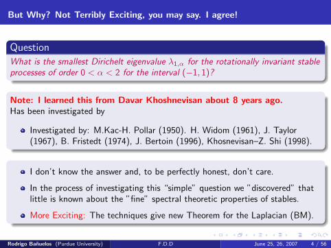
But Why? Not Terribly Exciting, you may say. I agree!

QuestionWhat is the smallest Dirichelt eigenvalue λ1,α for the rotationally invariant stableprocesses of order 0 < α < 2 for the interval (−1, 1)?

Note: I learned this from Davar Khoshnevisan about 8 years ago.Has been investigated by

Investigated by: M.Kac-H. Pollar (1950). H. Widom (1961), J. Taylor(1967), B. Fristedt (1974), J. Bertoin (1996), Khosnevisan–Z. Shi (1998).

I don’t know the answer and, to be perfectly honest, don’t care.

In the process of investigating this “simple” question we ”discovered” thatlittle is known about the ”fine” spectral theoretic properties of stables.

More Exciting: The techniques give new Theorem for the Laplacian (BM).


Best known bounds for λ1,α

R.B.and R. Latala and P. Mendez (2001) and R.B.and T. Kulczycki (2004)

Cα,d =Γ( d

2 )

2αΓ(1 + d2 )Γ( d+α

2 )

B(0, 1) = unit ball in Rd .

1

Cα,d≤ λ1,α(B(0, 1)) ≤ 1

Cα,d

B(d/2, α/2 + 1)

B(α/2, α + 1)

For α = 1 (Cauchy processes), B(0, 1) = (−1, 1) (as in Davar’s question)

1 ≤ λ1,1 ≤3π

8≈ 1.178

Note:3π

8<π

2=

√π2

4

That is, eigenvalue for Cauchy is not the square root of the one for

Brownian motion!


Variational Formula: For any D ⊂ Rd

The Dirichlet form, (E, F), for stables processes, 0 < α < 2, in Rd is:

E(f , g) = Aα,d

∫Rd

∫Rd

(f (x)− f (y))(g(x)− g(y))

|x − y |α+ddx dy

and

F =

{f ∈ L2(Rd) :

∫Rd

∫Rd

|f (x)− f (y)|2

|x − y |α+ddx dy <∞

}with

Aα,d =αΓ( d+α

2 )

21−απd/2Γ(1− α2 )


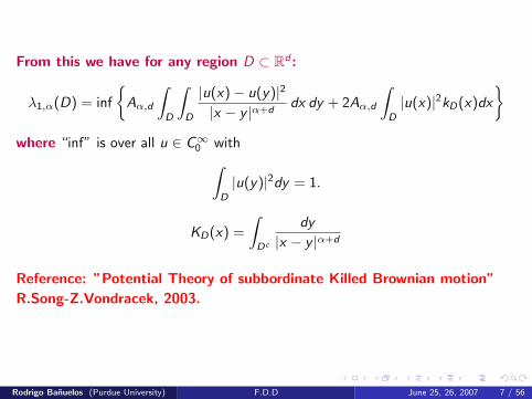
From this we have for any region D ⊂ Rd :

λ1,α(D) = inf

{Aα,d

∫D

∫D

|u(x)− u(y)|2

|x − y |α+ddx dy + 2Aα,d

∫D

|u(x)|2kD(x)dx

}where “inf” is over all u ∈ C∞0 with∫

D

|u(y)|2dy = 1.

KD(x) =

∫Dc

dy

|x − y |α+d

Reference: ”Potential Theory of subbordinate Killed Brownian motion”

R.Song-Z.Vondracek, 2003.


Eigenvalues and eigenfunctions enter into path properties of BM

Theorem (Chungs’s LIL. Set B∗t = sup0≤s≤t |Bs |)

lim inft→∞

(log log t

t

)1/2

B∗t =π

2, a.s. (1)

But, is π2 really just our good-old-friend π

2 or is it something else?(1) comes from Borel–Cantelli arguments and the “small balls” probabilityestimate: (See Bertoin,“Levy Processes” page 224, Banuelos–Moore,“Probabilistic behavior of harmonic functions,” Chapter 4.)

P0 {B∗1 < ε} ≈ e−π2

4ε2 , ε→ 0

P0 {B∗1 < ε} = P0

{1

εB∗t < 1

}= P0

{B∗1ε2< 1}

= P0

{τ(−1,1) >

1

ε2

}

τ(−1,1) = inf{t > 0 : Bt 6∈ (−1, 1)} = first exit time from the interval


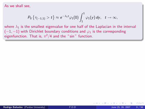
As we shall see,

P0

{τ(−1,1) > t

}≈ e−λ1tϕ1(0)

∫ 1

1

ϕ1(y) dy , t →∞,

where λ1 is the smallest eigenvalue for one half of the Laplacian in the interval(−1,−1) with Dirichlet boundary conditions and ϕ1 is the correspondingeigenfunction. That is, π2/4 and the “ sin ” function.

For any 0 < α < 2, let Xαt be the rotationally invariant stable process of order α.

A similar statement holds for the “small ball” probabilities and there is

Theorem (J. Taylor 1967)

lim inft→∞

(log log t

t

)1/α

X ∗t = (λ1,α)1/α, a.s. (2)

For several other occurrences of the eigenvalue in “sample path behavior,” seeErkan Nane: “Higher order PDE’s and iterated Processes” and “IteratedBrownian motion in bounded domains in Rn ”


Levy Processes

Constructed by Paul Levy in the 30’s (shortly after Wiener constructed Brownianmotion). Other names: de Finetti, Kolmogorov, Khintchine, Ito.

Rich stochastic processes, generalizing several basic processes in probability:Brownian motion, Poisson processes, stable processes, subordinators, . . .

Regular enough for interesting analysis and applications. Their paths consistof continuous pieces intermingled with jump discontinuities at random times.Probabilistic and analytic properties studied by many.

Many Developments in Recent Years:

Applied: Queueing Theory, Math Finance, Control Theory, PorousMedia . . .

Pure: Investigations on the “fine” potential and spectral theoreticproperties for subclasses of Levy processes


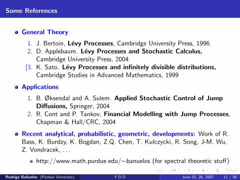
Some References

General Theory

1. J. Bertoin, Levy Processes, Cambridge University Press, 1996.2. D. Applebaum. Levy Processes and Stochastic Calculus,

Cambridge University Press, 2004[3. K. Sato. Levy Processes and infinitely divisible distributions,

Cambridge Studies in Advanced Mathematics, 1999

Applications

1. B. Øksendal and A. Sulem. Applied Stochastic Control of JumpDiffusions, Springer, 2004

2. R. Cont and P. Tankov, Financial Modelling with Jump Processes,Chapman & Hall/CRC, 2004

Recent analytical, probabilistic, geometric, developments: Work of R.Bass, K. Burdzy, K. Bogdan, Z.Q. Chen, T. Kulczycki, R. Song, J-M. Wu,Z. Vondracek, . . .

http://www.math.purdue.edu/∼banuelos (for spectral theoretic stuff)


Definition

A Levy Process is a stochastic process X = (Xt), t ≥ 0 with

X has independent and stationary increments

X0 = 0 (with probability 1)

X is stochastically continuous: For all ε > 0,

limt→s

P{|Xt − Xs | > ε} = 0

Note: Not the same as a.s. continuous paths. However, it gives“cadlag” paths: Right continuous with left limits.


Stationary increments: 0 < s < t <∞, A ∈ Rd Borel

P{Xt − Xs ∈ A} = P{Xt−s ∈ A}

Independent increments: For any given sequence of ordered times

0 < t1 < t2 < · · · < tm <∞,

the random variables

Xt1 − X0, Xt2 − Xt1 , . . . ,Xtm − Xtm−1

are independent.

The characteristic function of Xt is

ϕt(ξ) = E(e iξ·Xt

)=

∫Rd

e iξ·xpt(dx) = (2π)d/2pt(ξ)

where pt is the distribution of Xt . Notation (same with measures)

f (ξ) =1

(2π)d/2

∫Rd

e ix·ξf (x)dx , f (x =1

(2π)d/2

∫Rd

e−ix·ξf (ξ)dξ


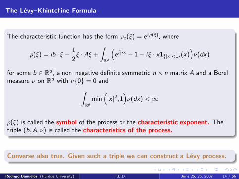
The Levy–Khintchine Formula

The characteristic function has the form ϕt(ξ) = etρ(ξ), where

ρ(ξ) = ib · ξ − 1

2ξ · Aξ +

∫Rd

(e iξ·x − 1− iξ · x1{|x|<1}(x)

)ν(dx)

for some b ∈ Rd , a non–negative definite symmetric n × n matrix A and a Borelmeasure ν on Rd with ν{0} = 0 and∫

Rd

min(|x |2, 1

)ν(dx) <∞

ρ(ξ) is called the symbol of the process or the characteristic exponent. Thetriple (b,A, ν) is called the characteristics of the process.

Converse also true. Given such a triple we can construct a Levy process.


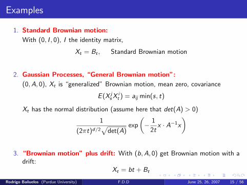
Examples

1. Standard Brownian motion:

With (0, I , 0), I the identity matrix,

Xt = Bt , Standard Brownian motion

2. Gaussian Processes, “General Brownian motion”:

(0,A, 0), Xt is “generalized” Brownian motion, mean zero, covariance

E (X js X i

t ) = aij min(s, t)

Xt has the normal distribution (assume here that det(A) > 0)

1

(2πt)d/2√

det(A)exp

(− 1

2tx · A−1x

)

3. “Brownian motion” plus drift: With (b,A, 0) get Brownian motion with adrift:

Xt = bt + Bt


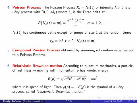
4. Poisson Process: The Poisson Process Xt = Nλ(t) of intensity λ > 0 is aLevy process with (0, 0, λδ1) where δ1 is the Dirac delta at 1.

P{Nλ(t) = m} =e−λt(λt)m

m!, m = 1, 2, . . .

Nλ(t) has continuous paths except for jumps of size 1 at the random times

τm = inf{t > 0 : Nλ(t) = m}

5. Compound Poisson Process obtained by summing iid random variables upto a Poisson Process.

6. Relativistic Brownian motion According to quantum mechanics, a particleof rest mass m moving with momentum p has kinetic energy

E (p) =√

m2c4 + c2|p|2 −mc2

where c is speed of light. Then ρ(p) = −E (p) is the symbol of a Levyprocess, called “relativistic Brownian motion.”


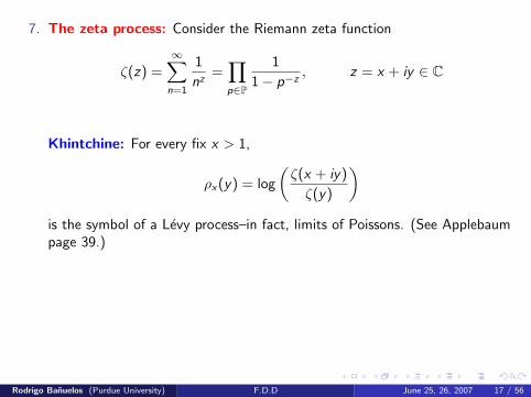
7. The zeta process: Consider the Riemann zeta function

ζ(z) =∞∑

n=1

1

nz=∏p∈P

1

1− p−z, z = x + iy ∈ C

Khintchine: For every fix x > 1,

ρx(y) = log

(ζ(x + iy)

ζ(y)

)is the symbol of a Levy process–in fact, limits of Poissons. (See Applebaumpage 39.)

Biane–Pitman-Yor: “Probability laws related to the Jacobi theta andRiemann Zeta functions and Brownian excursions, Bull. Amer math. Soc.,2001.

M Yor: A note about Selberg’s integrals with relation with the beta–gammaalgebra, 2006.


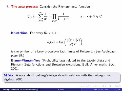
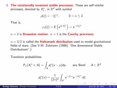
8. The rotationally invariant stable processes: These are self–similarprocesses, denoted by Xα

t , in Rd with symbol

ρ(ξ) = −|ξ|α, 0 < α ≤ 2.

That is,

ϕt(ξ) = E(

e iξ·Xαt)

= e−t|ξ|α

α = 2 is Brownian motion. α = 1 is the Cauchy processes.

α = 3/2 is called the Haltsmark distribution used to model gravitationalfields of stars. (See V.M. Zolotarev (1986) “One dimensional StableDistributions”.)

Transition probabilities:

Px{Xαt ∈ A} =

∫A

pαt (x − y)dy , any Borel A ⊂ Rd

pαt (x) =1

(2π)d

∫Rd

e−iξ·xe−t|ξ|αdξ


p2t (x) =

1

(4πt)d/2e−|x|24t , α = 2, Brownian motion

p1t (x) =

Cd t

(|x |2 + t2)d+1

2

, α = 1, Cauchy Process

For any a > 0, the two processes

{η(at) ; t ≥ 0} and {a1/αηt ; t ≥ 0},

have the same finite dimensional distributions (self-similarity).

In the same way, the transition probabilities scale similarly to those forBM:

pαt (x) = t−d/αpα1 (t−1/αx)


9. Subordinators

A subordinator is a one-dimensional Levy process {Tt} such that

(i) Tt ≥ 0 a.s. for each t > 0

(ii) Tt1 ≤ Tt2 a.s. whenever t1 ≤ t2

Theorem (Bertoin, p.73: Laplace transforms)

E (e−λTt ) = e−tψ(λ), λ > 0,

ψ(λ) = bλ+

∫ ∞0

(1− e−λs

)ν(ds)

b ≥ 0 and the Levy measure satisfies ν(−∞, 0) = 0 and∫∞0

min(s, 1)ν(ds) <∞.ψ is called the Laplace exponent of the subordinator.

Example (α/2–Stable subordinator): ψ(λ) = λα/2, 0 < α < 2 gives the withb = 0 and

ν(ds) =α/2

Γ(1− α/2)s−1−α/2 ds

Example 2 (Relativistic stable subordinator): 0 < α < 2 and m > 0,Ψ(λ) = (λ+ m2/α)α/2 −m.

ν(ds) =α/2

Γ(1− α/2)e−m2/αs s−1−α/2ds


ν(ds) =α/2

Γ(1− α/2)e−m2/αs s−1−α/2ds

Example 3 (Gamma subordinator): Ψ(λ) = log(1 + λ).

ν(ds) =e−s

sds

Many others: “Geometric stable subordinators, iterated geometric stablesubordinators, Bessel subordinators,. . . ”

Theorem (Applebaum, p. 53)

If X is an arbitrary Levy process and T is a subordinator independent of X ,then Zt = XTt is a Levy process. For any Borel A ⊂ Rd ,

pZt (A) =

∫ ∞0

pXs (A)pTt (ds)

When Xt = Bt Brownian motion, Zt is called subordinate Brownian motion.When Tt is the α/2 stable subordinator and X is BM, Z is the α rotationallyinvariant stable process of Example 8.


Levy semigroup

For the Levy process {X (t); t ≥ 0}, define

Tt f (x) = E [f (X (t))|X0 = x ] = E0[f (X (t) + x)], f ∈ S(Rd).

This is a Feller semigroup (takes C0(Rd) into itself). Setting

pt(A) = P0 {Xt ∈ A} (the distribution of Xt)

we see that (by Fourier inversion formula)

Tt f (x) =

∫Rd

f (x + y)pt(dy) = pt ∗ f (x) =1

(2π)d

∫Rd

e−ix·ξetρ(ξ) f (ξ)dξ

with generator

Af (x) =∂Tt f (x)

∂t

∣∣∣t=0

= limt→0

1

t

(Ex [f (X (t)]− f (x)

)=

1

(2π)d

∫Rd

e−ix·ξρ(ξ)f (ξ)dξ = a pseudo diff operator, in general


From the Levy–Khintchine formula (and properties of the Foruier transform),

Af (x) =∑i=1

bi∂i f (x) +1

2

∑i,j

ai,j∂i∂j f (x)

+

∫ [f (x + y)− f (x)− y · ∇f (x)χ{|y |<1}

]ν(dy)

Examples:

Standard Brownian motion:

Af (x) =1

2∆f (x)

Poisson Process of intensity λ:

Af (x) = λ[f (x + 1)− f (x)

]Rotationally Invariant Stable Processes of order 0 < α < 2, FractionalDiffusions:

Af (x) = −(−∆)α/2f (x)

= Aα,d

∫f (y)− f (x)

|x − y |d+αdy


Many questions on the “fine” potential theoretic properties of solutions for(−∆)α/2 have been studied by many authors in recent years. Examples:

Regularity of heat kernels, general solutions of “heat equation”, Sobolev,log-Sobolev inequalities, “intrinsic ultracontractivity,” . . .

“Boundary” regularity of solutions, including boundary Harnack principle,“gauge theorems,” Fatou theorems, Martin boundary, . . .

(1) “Potential theory of suborndinate BM,” (2007), Song-Vondracek(2) “Potential Theory for Levy Processes,” (2002) Bogdan–Stozs–Sztonyk.(3) “Multidimensional symmetric stable processes,”(1999), Z.Q. Chen(4) Also, have a look at the references given in the above papers and search forother recent papers of the authors already mentioned.

I am interested in the “fine” spectral theoretic properties of these processes

Estimates on eigenvalues, including the ground state λ1,α and the spectralgap λ2,α − λ1,α, Number of “nodal” domains (Courant–Hilbert Nodaldomain Theorem), geometric properties of eigenfunctions, including a“Brascamp–Lieb” log–concavity type theorem for ϕ1,α, . . .


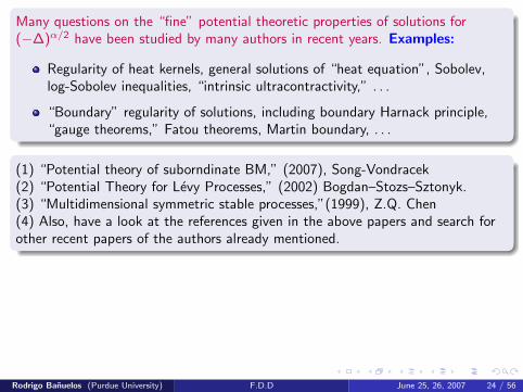
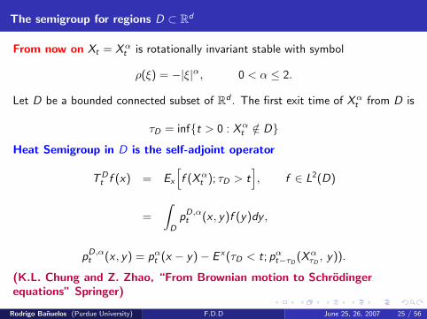
The semigroup for regions D ⊂ Rd

From now on Xt = Xαt is rotationally invariant stable with symbol

ρ(ξ) = −|ξ|α, 0 < α ≤ 2.

Let D be a bounded connected subset of Rd . The first exit time of Xαt from D is

τD = inf{t > 0 : Xαt /∈ D}

Heat Semigroup in D is the self-adjoint operator

T Dt f (x) = Ex

[f (Xα

t ); τD > t], f ∈ L2(D)

=

∫D

pD,αt (x , y)f (y)dy ,

pD,αt (x , y) = pαt (x − y)− E x(τD < t; pαt−τD

(XατD, y)).

(K.L. Chung and Z. Zhao, “From Brownian motion to Schrodingerequations” Springer)


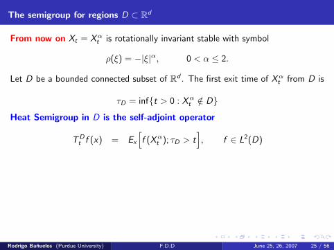
pD,αt (x , y) is called the Heat Kernel for the stable process in D.

pD,αt (x , y) ≤ pαt (x − y) ≤ pα1 (0)t−d/α =

(1

(2π)d

∫Rd

e−|ξ|α

dξ

)t−d/α

= t−d/α ωd

(2π)dα

∫ ∞0

e−ss( nα−1)ds

= t−d/α ωdΓ(d/α)

(2π)dα

The general theory of heat semigroups (R. Bass “Probabilistic Techniques inAnalysis,” B. Davies, “Heat Semigroups”) gives an orthonormal basis ofeigenfunctions

{ϕm,α}∞m=1 on L2(D)

with eigenvalues {λm,α} satisfying

0 < λ1,α < λ2,α ≤ λ3,α ≤ · · · → ∞

That is,

T Dt ϕm,α(x) = e−λm,αtϕm,α(x), x ∈ D.


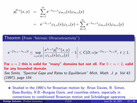
pD,αt (x , y) =

∞∑m=1

e−λm,αtϕm,α(x)ϕm,α(y)

= e−λ1,αtϕ1,α(x)ϕ1,α(y) +∞∑

m=2

e−λm,αtϕm,α(x)ϕm,α(y)

Theorem (From “Intrinsic Ultracontractivity”)

e−(λ2,α−λ1,α)t ≤ supx,y∈D

∣∣∣∣∣eλ1,αtpD,αt (x , y)

ϕ1,α(x)ϕ1,α(y)− 1

∣∣∣∣∣ ≤ C (D, α)e−(λ2,α−λ1,α)t , t ≥ 1.

For α = 2 this is valid for “many” domains but not all. For 0 < α < 2, validfor any bounded domain.See Smits, “Spectral Gaps and Rates to Equilibrium” Mich. Math. J. p. Vol 43(1997), page 154.

Studied in the 1990’s for Brownian motion by: Brian Davies, B. Simon,Bass-Burdzy, R.B.–Burgess Davis, and countless others, especially inconnections to conditioned Brownian motion and Schrodinger operators.

Studied for stables in late 90’s early 2000’s by: Z.Q. Chen, R. Song, K.Bogdan, T. Kulczycki, J. Wu, . . .


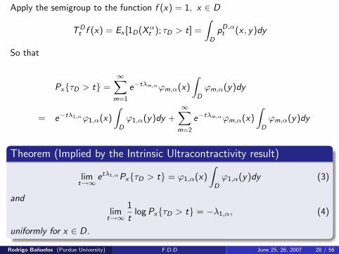
Apply the semigroup to the function f (x) = 1, x ∈ D

T Dt f (x) = Ex [1D(Xα

t ); τD > t] =

∫D

pD,αt (x , y)dy

So that

Px{τD > t} =∞∑

m=1

e−tλm,αϕm,α(x)

∫D

ϕm,α(y)dy

= e−tλ1,αϕ1,α(x)

∫D

ϕ1,α(y)dy +∞∑

m=2

e−tλm,αϕm,α(x)

∫D

ϕm,α(y)dy

Theorem (Implied by the Intrinsic Ultracontractivity result)

limt→∞

etλ1,αPx{τD > t} = ϕ1,α(x)

∫D

ϕ1,α(y)dy (3)

and

limt→∞

1

tlog Px{τD > t} = −λ1,α, (4)

uniformly for x ∈ D.


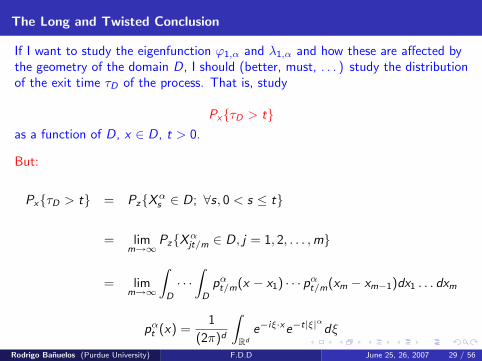
The Long and Twisted Conclusion

If I want to study the eigenfunction ϕ1,α and λ1,α and how these are affected bythe geometry of the domain D, I should (better, must, . . . ) study the distributionof the exit time τD of the process. That is, study

Px{τD > t}as a function of D, x ∈ D, t > 0.

But:

Px{τD > t} = Pz{Xαs ∈ D; ∀s, 0 < s ≤ t}

= limm→∞

Pz{Xαjt/m ∈ D, j = 1, 2, . . . ,m}

= limm→∞

∫D

· · ·∫

D

pαt/m(x − x1) · · · pαt/m(xm − xm−1)dx1 . . . dxm

pαt (x) =1

(2π)d

∫Rd

e−iξ·xe−t|ξ|αdξ


In the same way (integrating against a delta function at y)

pD,αt (x , y) = lim

m→∞

∫D

· · ·∫

D

pαt/m(x − x1) · · · pαt/m(y − xm−1)dx1 . . . dxm−1,

Alternatively, for Brownian motion, if 0 = t0 < t1 < . . . < tm < t, then theconditional finite-dimensional distribution

Pz0{Bt1 ∈ dx1, . . . ,Btm ∈ dxm |Bt = y},

is given byp2

t−tm (zn, y)

p2t (z0, y)

m∏i=1

p2ti−ti−1

(zi , zi−1),

Reference:

I. Karatzas and E. Shreve, Brownian Motion and Stochastic Calculus,Springer-Verlang, New York, 1991–page 395.

Similar formula holds for ”stable bridges”, Bertoin, page 226.


Do we really need the stables?

With Xαt = BTt with

E (e−λTt ) = e−tλα/2

, λ > 0,

we have

pαt (x) =

∫ ∞0

p(2)s (x) gα/2(t, s)ds =

∫ ∞0

1

(4πs)d/2e|x|

2/4sgα/2(t, s) ds

wheregα/2(t, s) = density of Tt

Note: α = 1/2,

Tt = inf{s > 0 : Bs =t√2}

and

g1/2(t, s) =

(t

2√π

)s−3/2e−t2/4s , Bochner subordination


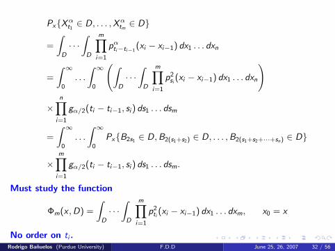
Px{Xαt1 ∈ D, . . . ,Xα

tm ∈ D}

=

∫D

· · ·∫

D

m∏i=1

pαti−ti−1(xi − xi−1) dx1 . . . dxn

=

∫ ∞0

. . .

∫ ∞0

(∫D

· · ·∫

D

m∏i=1

p2si

(xi − xi−1) dx1 . . . dxn

)

×n∏

i=1

gα/2(ti − ti−1, si ) ds1 . . . dsm

=

∫ ∞0

. . .

∫ ∞0

Px{B2s1 ∈ D,B2(s1+s2) ∈ D, . . . ,B2(s1+s2+···+sn) ∈ D}

×m∏

i=1

gα/2(ti − ti−1, si ) ds1 . . . dsm.

Must study the function

Φm(x ,D) =

∫D

· · ·∫

D

m∏i=1

p2ti (xi − xi−1) dx1 . . . dxm, x0 = x

No order on ti .Rodrigo Banuelos (Purdue University) F.D.D June 25, 26, 2007 32 / 56

For A ⊂ Rd , A∗ =ball centered at the origin and same volume as A. χ∗A = χA∗

f : Rd → R,

f ∗(x) =

∫ ∞0

χ∗{|f |>t}(x)dt

(Compare this with)

|f (x)| =

∫ ∞0

χ{|f |>t}(x)dt

Properties:

f ∗(x) = f ∗(y), |x | = |y |, f ∗(x) ≥ f ∗(y), |x | ≤ |y |

{x : f ∗(x) > t} = {x : |f (x)| > t}∗ (same level sets)

⇒ m{x : f ∗(x) > λ} = m{x : |f (x)| > λ}


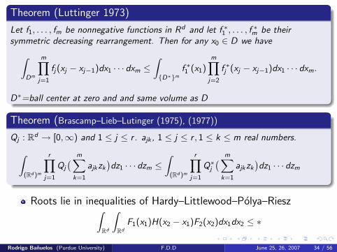
Theorem (Luttinger 1973)

Let f1, . . . , fm be nonnegative functions in Rd and let f ∗1 , . . . , f∗m be their

symmetric decreasing rearrangement. Then for any x0 ∈ D we have∫Dm

m∏j=1

fj(xj − xj−1)dx1 · · · dxm ≤∫{D∗}m

f ∗1 (x1)m∏

j=2

f ∗j (xj − xj−1)dx1 · · · dxm.

D∗=ball center at zero and and same volume as D

Theorem (Brascamp–Lieb–Lutinger (1975), (1977))

Qj : Rd → [0,∞) and 1 ≤ j ≤ r . ajk , 1 ≤ j ≤ r , 1 ≤ k ≤ m real numbers.∫(Rd )m

r∏j=1

Qj

( m∑k=1

ajkzk

)dz1 · · · dzm ≤

∫(Rd )m

r∏j=1

Q∗j( m∑

k=1

ajkzk

)dz1 · · · dzm

Roots lie in inequalities of Hardy–Littlewood–Polya–Riesz∫Rd

∫Rd

F1(x1)H(x2 − x1)F2(x2)dx1dx2 ≤ ∗


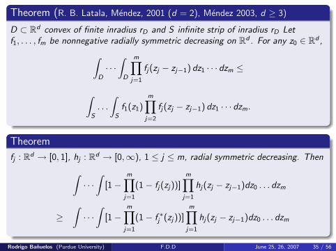
Theorem (R. B. Latala, Mendez, 2001 (d = 2), Mendez 2003, d ≥ 3)

D ⊂ Rd convex of finite inradius rD and S infinite strip of inradius rD Letf1, . . . , fm be nonnegative radially symmetric decreasing on Rd . For any z0 ∈ Rd ,∫

D

· · ·∫

D

m∏j=1

fj(zj − zj−1) dz1 · · · dzm ≤

∫S

. . .

∫S

f1(z1)m∏

j=2

fj(zj − zj−1) dz1 · · · dzm.

Theorem

fj : Rd → [0, 1], hj : Rd → [0,∞), 1 ≤ j ≤ m, radial symmetric decreasing. Then∫· · ·∫

[1−m∏

j=1

(1− fj(zj))]m∏

j=1

hj(zj − zj−1)dz0 . . . dzm

≥∫· · ·∫

[1−m∏

j=1

(1− f ∗j (zj))]m∏

j=1

hj(zj − zj−1)dz0 . . . dzm


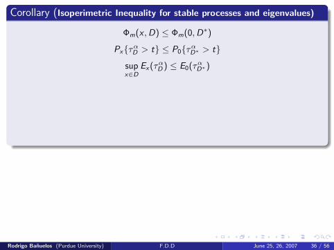
Corollary (Isoperimetric Inequality for stable processes and eigenvalues)

Φm(x ,D) ≤ Φm(0,D∗)

Px{ταD > t} ≤ P0{ταD∗ > t}

supx∈D

Ex(ταD ) ≤ E0(ταD∗)

λ1,α(D∗) ≤ λ1,α(D) The Faber-Krahn Theorem

Capα(A) ≥ Capα(A∗),

(α-capacity version of a theorem of Polya–Szego. Proved by Watanabe 1984,conjectured by Mattila 1990, Proved by Betsakos 2003, P. Mendez 2006)

Corollary (Isoperimetric Inequality for the “partition function”)

Zαt (D) =

∞∑m=1

e−tλm,α(D) =

∫D

pα,Dt (x , x)dx

≤∫

D∗pα,D

∗

t (x , x)dx ≤∞∑

m=1

e−tλm,α(D∗) = Zαt (D∗)


Classical Isoperimetric Inequality

Amongst all regions of equal volume the ball minimizes surface area. Itfollows from ”trace inequality” and

Theorem (M. Kac, “Can one hear the shape of a drum?”)

With α = 2, |∂D|=surface area of boundary of D,

Z 2t (D) ∼ Cd t−d/2vol(D)− C ′d t−(d−1)/2|∂D|+ o(t−(d−1)/2, t → 0

The first term is trivial from

P2,Dt (x , y) =

1

(4πt)d/2e−|x−y|2

4t Px{τD > t|Bt = y}

= free motion times Brownian bridge in D


A detour into Weyl’s asymptotics

limt→0

tγ∫ ∞

0

e−tλdµ(λ) = A⇒ lima→∞

a−γµ[0, a) =A

Γ(γ + 1)

Theorem (Weyl’s Formula, α = 2. ND(λ) = #{j ≥ 1 : λj ≤ λ})

ND(λ) ∼ Cdvol(D)λd/2, λ→∞

More difficult (and no probabilistic treatment exists):

ND(λ) ∼ Cdvol(D)λd/2 − C ′d |∂D|λ(d−1)/2 + o(λ(d−1)/2)

Theorem (R.B. and T. Kulczycki (2007). 0 < α ≤ 2)∫D

pα,Dt (x , x)dx ∼ Cd,αt−d/αvol(D)− C ′d t−(d−1)/α|∂D|+ o(t−(d−1)/α

as t → 0. This gives Weyl’s version for all 0 < α ≤ 2.The $$ Question: Is there an α–version of the more general Weyl?


Back on main road: Fixing other parameters besides volume

Question

Amongst all convex domains D ⊂ Rd of inradius 1, which one has the largest exittime for Brownian motion? Also, lowest eigenvalue? Answer:The infinite strip:

S = Rd−1 × (−1, 1)

Theorem (For D convex with inradius 1.)

Φm(x ,D) ≤ Φm(0,S), x ∈ D

R.B. Mendez-Latala (2001), d = 2 and (2003), d ≥ 3. (Convexity is essentialhere!)

Corollary (For D convex with inradius 1 and 0 < α ≤ 2.)

Px{τD > t} ≤ P0{τS > t} = P0{τ(−1,1) > t} (5)

λ1,α(−1, 1) ≤ λ1,α(D) (6)


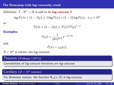
The Brascamp–Lieb log–concavity result

Definition: F : Rd → R is said to be log-concave if

log F (βx + (1− β)y) ≥ β log F (x) + (1− β) log F (y), x , y ∈ Rd

orF (βx + (1− β)y) ≥ F (x)βF (y)1−β

Examples:

F (x) =1

(4π)d/2e−|x|

2/4

andF (x) = χD(x),

D ⊂ Rd is convex, are log–concave.

Theorem (Prekopa (1971))

Convolutions of log-concave functions are log-concave.

Corollary (D ⊂ Rd convex)

For Brownian motion, the function Φm(x ,D) is log-concave.


Corollary (Brascamp-Lieb (1979))

For any bounded convex domain D ⊂ Rd and for Brownian motion, thefunction Px{τD > t} is log-concave and therefore so is the “ground state”eigenfunction ϕ1,2(x). In fact, this holds for the “ground state”eigenfunction for the Scrodinger operator −∆ + V where V : D → [0,∞) isconvex.

Note: Unfortunately we cannot conclude the same for 0 < α < 2. Why?

Question (D ⊂ Rd convex, 0 < α < 2)

Are the functions Px{τD > t} and/or ϕ1,α(x) log-convex?

Known only for α = 1, D = (−1, 1). In fact, in this case the functions areconcave, just like for α = 2.

Several other partial results are known for special doubly symmetricdomains in the plane.


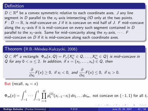
Definition

D ⊂ Rd be a convex symmetric relative to each coordinate axes. J any linesegment in D parallel to the x1-axis intersecting ∂D only at the two points.F : D → R, is mid–concave on J if it is concave on mid half of J. F mid–concavealong the x1–axis if it is mid–concave on every such segment contained in Dparallel to the x1–axis. Same for mid–concavity along the x2-axis, · · · . Fmid–concave on D if it is mid–concave along each coordinate axes.

Theorem (R.B.-Mendez-Kulczycki, 2006)

Q ⊂ Rd a rectangle. Φm(x ,Q) = Px{Xαt1 ∈ Q, . . . ,Xα

tm ∈ Q} is mid–concave inQ for any 0 < α ≤ 2. In addition, if x = (x1, . . . , xn) ∈ Q, then

∂

∂xiF (x) ≥ 0, if xi < 0, and

∂

∂xiF (x) ≤ 0, if xi > 0.

But (recall, x0 = x)

Φm(x) =

∫ 1

−1

· · ·∫ 1

−1

m∏i=1

p(2)ti (xi−1−xi ) dx1 . . . dxm, not concave on (−1, 1) for all ti .


Corollary

Let Q = (−a1, a1)× (−a2, a2)× · · · × (−ad , ad), 0 < ai <∞ for alli = 1, 2, . . . , d, be a rectangle in Rd . ϕ1,α 0 < α < 2 is mid–concave on Q. Inaddition, if x = (x1, . . . , xn) ∈ Q, then

∂

∂xiϕα1 (x) ≥ 0, if xi < 0, and

∂

∂xiϕα1 (x) ≤ 0, if xi > 0.

TheoremFor n ≥ 1, set

D(n) =

{(x1, x2) ∈ R2 : x1 ∈ (−n, n), x2 ∈

(−1 +

|x1|n, 1− |x1|

n

)}.

For n large enough, ϕ1,2 is not mid–concave on D(n).


Why is log-concavity important?

Probabilistic reasons: Many people (C. Borell, S. Bobkov, C. Houdre, M.Ledoux) have studied ”isoperimetric inequalties” ”Cheeger’s inequalities”,etc., for log–concave measures. Here is a ”beautiful result:” For anyprobability measure µ on Rd define its “spectral gap” by

Specg(µ) = inff∈Lip(1)

{∫Rd |∇f |2dµ∫Rd |f |2dµ

:

∫Rd

f dµ = 0

}

Theorem (Bobkov 1996)

Suppose dµ = f (x)dx, f log-concave and diam(µ) = diam(supp(f )) <∞. Then

Specg(µ) ≥ c

diam2(µ)

Theorem (R. Smits 1997. Under same assumptions as Bobkov)

Specg(µ) ≥ π2

diam2(µ)


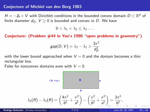
Conjecture of Michiel van den Berg 1983

H = −∆ + V with Dirichlet conditions in the bounded convex domain D ⊂ Rd offinite diameter dD , V ≥ 0 is bounded and convex in D. We have

0 < λ1 < λ2 ≤ λ3 . . . .

Conjecture: (Problem #44 in Yau’s 1990 “open problems in geometry”)

gap(D,V ) = λ2 − λ1 >3π2

d2D

with the lower bound approached when V = 0 and the domain becomes a thinrectangular box.False for nonconvex domains even with V = 0.

aR

b

( b > a )

λ2(R)− λ1(R) =

(4π2

b2+π2

a2

)−(π2

b2+π2

a2

)=

3π2

b2,


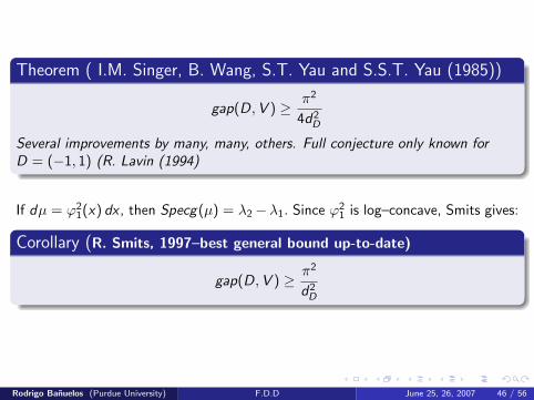
Theorem ( I.M. Singer, B. Wang, S.T. Yau and S.S.T. Yau (1985))

gap(D,V ) ≥ π2

4d2D

Several improvements by many, many, others. Full conjecture only known forD = (−1, 1) (R. Lavin (1994)

If dµ = ϕ21(x) dx , then Specg(µ) = λ2−λ1. Since ϕ2

1 is log–concave, Smits gives:

Corollary (R. Smits, 1997–best general bound up-to-date)

gap(D,V ) ≥ π2

d2D


Take V = 0 for now. (A. Melas, 1998 UCLA Ph.D Thesis. The “nodaldomains” for ϕ2 look like in the picture)

(D

D

Domain D

_D

+

φ2 < 0 φ2 > 0

φ2(D)= φ

(D)=λ 2 (Dλ

1

1

)

+)

+

More General Conjecture: D convex of diameter dD . Let

I = (−dD

2,

dD

2), I + = (0,

dD

2)

∫D+ PD+

t (z , z)dz∫D

PDt (z , z)dz

≤∫I+ P I+

t (z , z)dz∫I

P It (z , z)dz


Conjecture Equivalent to (In terms of Partition Function):

Z 2t (D+)

Z 2t (D)

=

∑∞j=1 e−tλj (D

+)∑∞j=1 e−tλj (D)

≤∑∞

j=1 e−tλj (I+)∑∞

j=1 e−tλj (I )=

Z 2t (I +)

Z 2t (I )

L. Payne (here at Cornell) (1973)

Nodal line either: a)

b)or


R+

D+

a

-a

(x, 0) -b

Symmetric in y, Convex in x D={(x, y): -a <y < a, -f(y) <x < f(y)}

b..

..w* w

Theorem (R.B. Medez-Hernandez, 2002)

Suppose D, and D+ and b are as in the picture.

P(x,0){τD+ > t}P(x,0){τD > t}

≤Px{τ(0,b) > t}

Px{τ(−b,b) > t}

Same as:Φm(D+, (x , 0))

Φm(D, (x , 0))≤ Φm((0, b), x)

Φm((−b, b), x)(F.D.D., again!)


Theorem about Brownian motion in cylinders

D

Two domains in

3-dimensions:

and

eigenvalue?

Which Half has the

Right Half

Bottom Half

smallest Dirichlet

Diameter= Height

D- symmetric relative to y


”Hot–spots” conjecture of Jeff Rauch (University of Michigan)–1973

The maximum (and the minimum) of the “first” non-constant Neumanneigenfunction for bounded convex domains are attained on the boundaryand only on the boundary of the domain.

Many partial results: R.B.-K.Burdzy (1999), D.Jerison-N.Darishavilli(2000), M. Pascu (2001), R. Bass–K. Burdzy (2000), R.B.-M. Pang(2003), R.B. M.Pang-Pascu (2004), R.Atar K.Burdzy (2005)

Counterexample: K. Burdzy-W. Werner (2000), K. Burdzy (2005)

Believed to be true for any simply connected domain, conjectured to betrue for any convex domain.

Unknown even for an arbitrary triangle in the plane!


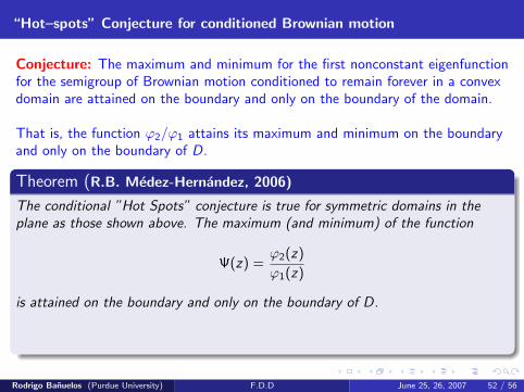
“Hot–spots” Conjecture for conditioned Brownian motion

Conjecture: The maximum and minimum for the first nonconstant eigenfunctionfor the semigroup of Brownian motion conditioned to remain forever in a convexdomain are attained on the boundary and only on the boundary of the domain.

That is, the function ϕ2/ϕ1 attains its maximum and minimum on the boundaryand only on the boundary of D.

Theorem (R.B. Medez-Hernandez, 2006)

The conditional ”Hot Spots” conjecture is true for symmetric domains in theplane as those shown above. The maximum (and minimum) of the function

Ψ(z) =ϕ2(z)

ϕ1(z)

is attained on the boundary and only on the boundary of D.

Proof: Via finite dimensional distributions!


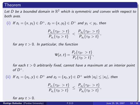
Theorem

Let D be a bounded domain in R2 which is symmetric and convex with respect toboth axes.

(i) If z1 = (x , y1) ∈ D+, z2 = (x , y2) ∈ D+ and y1 < y2, then

Pz1{τD+ > t}Pz1{τD > t}

<Pz2{τD+ > t}Pz2{τD > t}

,

for any t > 0. In particular, the function

Ψ(z , t) =Pz{τD+ > t}Pz{τD > t}

,

for each t > 0 arbitrarily fixed, cannot have a maximum at an interior pointof D+.

(ii) If z1 = (x1, y) ∈ D+ and z2 = (x2, y) ∈ D+ with |x2| ≤ |x1|, then

Pz1{τD+ > t}Pz1{τD > t}

≤ Pz2{τD+ > t}Pz2{τD > t}

,

for any t > 0.Rodrigo Banuelos (Purdue University) F.D.D June 25, 26, 2007 53 / 56

Corollary

D ⊂ R2 as in Theorem ϕ2 be such that its nodal line is the intersection of thex-axis with the domain. Without LOG, ϕ2 > 0 in D+ and ϕ2 < 0 in D−. SetΨ = ϕ2/ϕ1.

(i) If z1 = (x , y1) ∈ D+ and z2 = (x , y2) ∈ D+ with y1 < y2, then

Ψ(z1) < Ψ(z2).

(ii) If z1 = (x , y1) ∈ D− and z2 = (x , y2) ∈ D− with y2 < y1, then

Ψ(z1) < Ψ(z2).

In particular, Ψ cannot attain a maximum nor a minimum in the interior ofD.

(iii) If z1 = (x1, y) ∈ D+ and z2 = (x2, y) ∈ D+ with |x2| < |x1|, then

Ψ(z1) ≤ Ψ(z2). (7)


Corollary (Exact analogue of D. Jerison and N. Nadirashvili (2000) for classical“hot–spots”)

Suppose D ⊂ R2 is a bounded domain with piecewise smooth boundary which issymmetric and convex with respect to both coordinate axes and that ϕ2 is as inTheorem 1.2. Then strict inequality holds in (7) unless D is a rectangle. Themaximum and minimum of Ψ on D are achieved at the points where the y-axismeets ∂D and, except for the rectangle, at no other points.

Nodal line either: a)

b)or


“To a hammer everything is a nail”

Can finite dimensional distributions make my morning coffee?”

Mow my lawn?

don’t know that,. . .

yet!


Finite Dimensional Distributions. What can you do with them?

Documents

Transcript of Finite Dimensional Distributions. What can you do with them?