Finite Difference Method for PDE

1

Y V S S SanyasirajuProfessor, Department of MathematicsIIT Madras, Chennai 36

Classification of the Partial Differential Equations

• Consider a scalar second order partial differential equation(PDE) in ‘d ’ independent variables, given by

(4.1.1)

• Unless otherwise stated, repeated index stands for summation

• The stationary form of the Eq. (4.1.1) is given by

(4.1.2)

where , 0, , ,

T

d

L a b c st x x x

s T d

2

SL a b c sx x x

2

• Equation (4.1.2) is obtained after

– Renaming as bα and also using

– Further, the coefficients of the cross derivates are made equalby enforcing aαβ = aβα = 1/2 (aαβ + aβα).

• Arranging the coefficients aαβ (real) in a matrix form, say, A,gives a symmetric matrix of size (d x d) with real coefficients.

• Such a matrix will have d real eigenvalues and the correspondingeigenvectors are linearly independent.

3

x x x x ,xb aaa ba-

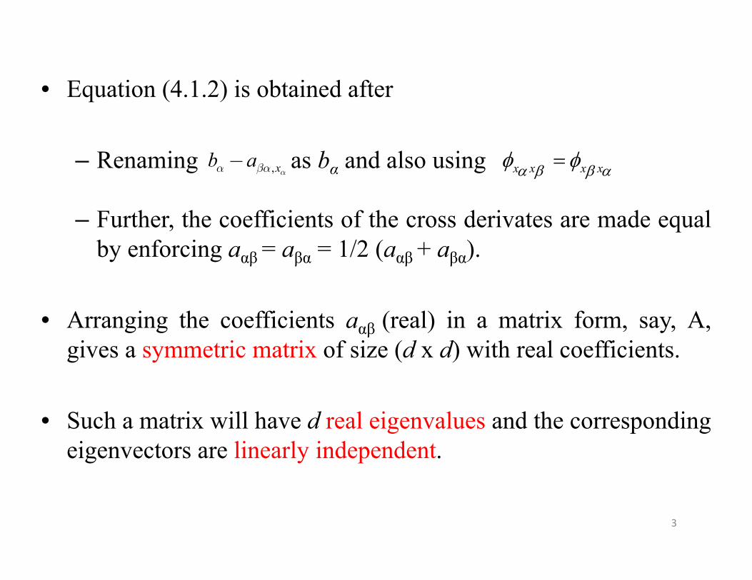
Classification• Differential equation (4.1.2) is called

– Elliptic if the eigenvalues of A are non-zero and have thesame sign

– Hyperbolic if only one eigenvalue has sign different from allothers

– Parabolic if precisely one eigenvalue is zero, while the otherhave the same sign and rank of (A, b) is equal to thedimension of the problem with the vector b has the elementsof bα.

• For the elliptic case, A is definite and can be treated as positivedefinite. If not, the equation can be multiplied with a minus one(-1) and can be made to Positive definite.

4

• Tensor form of second order partial differential equation, givenin (4.1.1) and (4.1.2), is good for classifying a PDE in ‘ d ’independent variables.

• However, for ‘d = 2’, it is easier to use the quasi-linear form ofequation (4.1.2), in its explicit form, given by

(4.13)

where A, B and C are functions of the independent variables xand y alone.

• Then the classification of the PDE (4.1.3) depends on the sign ofthe discriminant (B2-4AC). Notice that the coefficient of the firstderivative terms don’t contribute to the classifications

2 2 2

2 2( , ) ( , ) ( , ) 0A x y B x y C x y D E Fx x y y x y

5

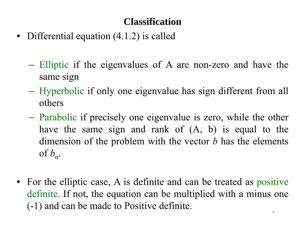
• Equation (4.1.3) is hyperbolic in the regions where thediscriminant is positive and is elliptic when it is negative. Theequation is called parabolic whenever (B2-4AC) is zero.

• Well known examples for elliptic, hyperbolic and parabolic PDEare :

Poisson’s equation

Wave equation and

Unsteady diffusion equation , respectively.

2 2

2 2 ( , )x

f x yy

2 22

2 2xc

t

2

2xK

t

6

Classification of Non – Stationary Equations

• For the transient case, a first derivative with respect to time is anadditional term when compared to the corresponding stationarydifferential equation.

• Since the first derivatives does not contribute to theclassification, the existing elements of A are same for bothstationary and transient cases.

• However, due to the increase of the number of independentvariables by one (time variable t), the number of rows andcolumns of A will increase by one with zero elements.

• This will result into an additional zero eigenvalue. 7

• Therefore, from the classification in terms eigenvalues, if thestationary equation is elliptic then the corresponding unsteadyequation is parabolic.

• The same in equation form can be written as

where AT and AS are the matrices with coefficients of the secondderivative terms of transient and stationary equations,respectively.

00 0 1s s

S T

A bL s A and b

t

8

Initial and Boundary Conditions

• Unsteady equations require initial conditions given by(4.1.4a)

• And the boundary conditions, on ∂Ω, (0 < t < T), which can beany one of the following:

(4.1.4b)

00, ( ), , 0x x x t

1. , ,

2. , ,

3. , , ,

Dirichlet t x f t x

Neumann K t x f t xn

Robin K t x a t x f t xn

9

• Indirectly boundary conditions play a very important role in theclassification of the PDE.

• For elliptic equations, the boundary conditions, which have to beprescribed all along the boundary of the domain, influence thesolution everywhere.

• For hyperbolic equations, a local change in the boundary datainfluences only a part of the domain resulting into a domain ofinfluence and domain of dependence. The CFL condition of thenumerical schemes used in CFD is based on this principle.

• Finally, for parabolic equations, a time like variable can beidentified and any changes in the boundary data influences theentire domain however only at the later times.

10

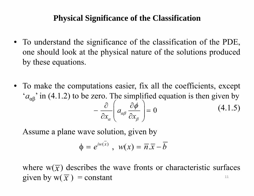
Physical Significance of the Classification

• To understand the significance of the classification of the PDE,one should look at the physical nature of the solutions producedby these equations.

• To make the computations easier, fix all the coefficients, except‘aαβ’ in (4.1.2) to be zero. The simplified equation is then given by

(4.1.5)

Assume a plane wave solution, given by

where w( ) describes the wave fronts or characteristic surfacesgiven by w( ) = constant

0ax x

( ) , ( ) .iw xe w x n x b

xx

11

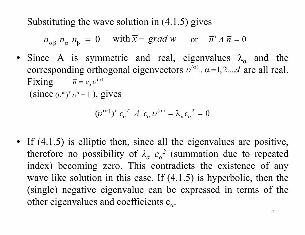
Substituting the wave solution in (4.1.5) gives

• Since A is symmetric and real, eigenvalues λα and thecorresponding orthogonal eigenvectors are all real.Fixing(since ), gives

• If (4.1.5) is elliptic then, since all the eigenvalues are positive,therefore no possibility of λα cα2 (summation due to repeatedindex) becoming zero. This contradicts the existence of anywave like solution in this case. If (4.1.5) is hyperbolic, then the(single) negative eigenvalue can be expressed in terms of theother eigenvalues and coefficients cα.

0a n n with x grad w or 0Tn A n

( ) , 1, 2....d ( )n c

( ) 1T

( ) ( ) 2( ) 0T Tc A c c

12

• That shows the existence of wave like solution for hyperbolictype equations.

• Finally, if (4.1.5) is parabolic then exactly one eigenvalue iszero, therefore one can fix the corresponding cα as non-zero andall the other coefficients to be zero. That is, one particulardirection can be identified in which wave like solution canexists.

• To conclude, there is no possibility of wave like solutions toexist for elliptic equations, however a clear case of existence ofwave like solutions, in any of the many directions, for thehyperbolic equations.

• And finally, existence of exactly one particular direction inwhich wavelike solutions may form for parabolic equations.

13

Convection – Diffusion Equation (CDE)

• A general convection – diffusion equation is given by

(4.1.13)

where ε is the constant diffusion parameter.

• For small values of ε, Eq. (4.1.13) has layer solutions (solutionvaries very rapidly in a small region(s) particularly towards anyphysical boundary of the problem).

• The study of Eq. (4.1.13), when the diffusion parameter issmall, is called the boundary layer theory or singularperturbation theory.

2

, , 0, 1,2,...,u s x t T dt x x x

14

• The stationary form of the convection-diffusion equation isgiven by

(4.1.14)

• The convection – diffusion equation which is also known asBurger’s equation is similar to some of the governing equationsof the fluid dynamics but without any pressure term.

• Further, due to the layer behavior of its solutions obtainingaccurate numerical solutions is a challenge

2

u sx x x

15

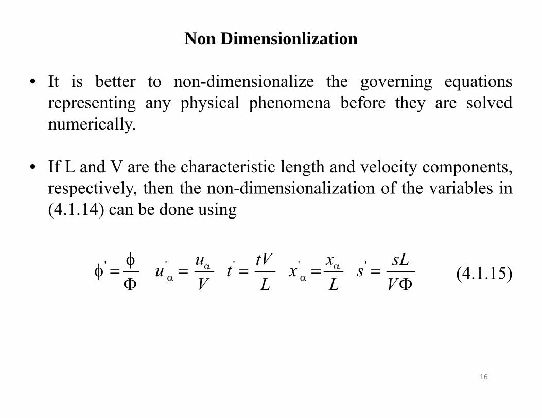
Non Dimensionlization

• It is better to non-dimensionalize the governing equationsrepresenting any physical phenomena before they are solvednumerically.

• If L and V are the characteristic length and velocity components,respectively, then the non-dimensionalization of the variables in(4.1.14) can be done using

(4.1.15)' ' ' ' 'u xtV sLu t x sV L L V

16

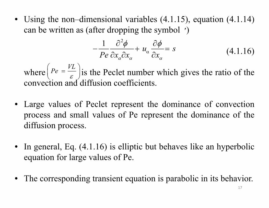
• Using the non–dimensional variables (4.1.15), equation (4.1.14)can be written as (after dropping the symbol ( ׳

(4.1.16)

where is the Peclet number which gives the ratio of theconvection and diffusion coefficients.

• Large values of Peclet represent the dominance of convectionprocess and small values of Pe represent the dominance of thediffusion process.

• In general, Eq. (4.1.16) is elliptic but behaves like an hyperbolicequation for large values of Pe.

• The corresponding transient equation is parabolic in its behavior.

21 u sPe x x x

VLPe

17

Discretization

• There are three steps in numerically solving the differentialequations:

1. Discretization of the domain by placing a large number ofnodes with help of grid generation techniques.

2. Approximating (or discretizing) the governing equations at thenodes identified in Step 1.

3. Solving the algebraic equations obtained in Step 2 using director iterative methods.

18

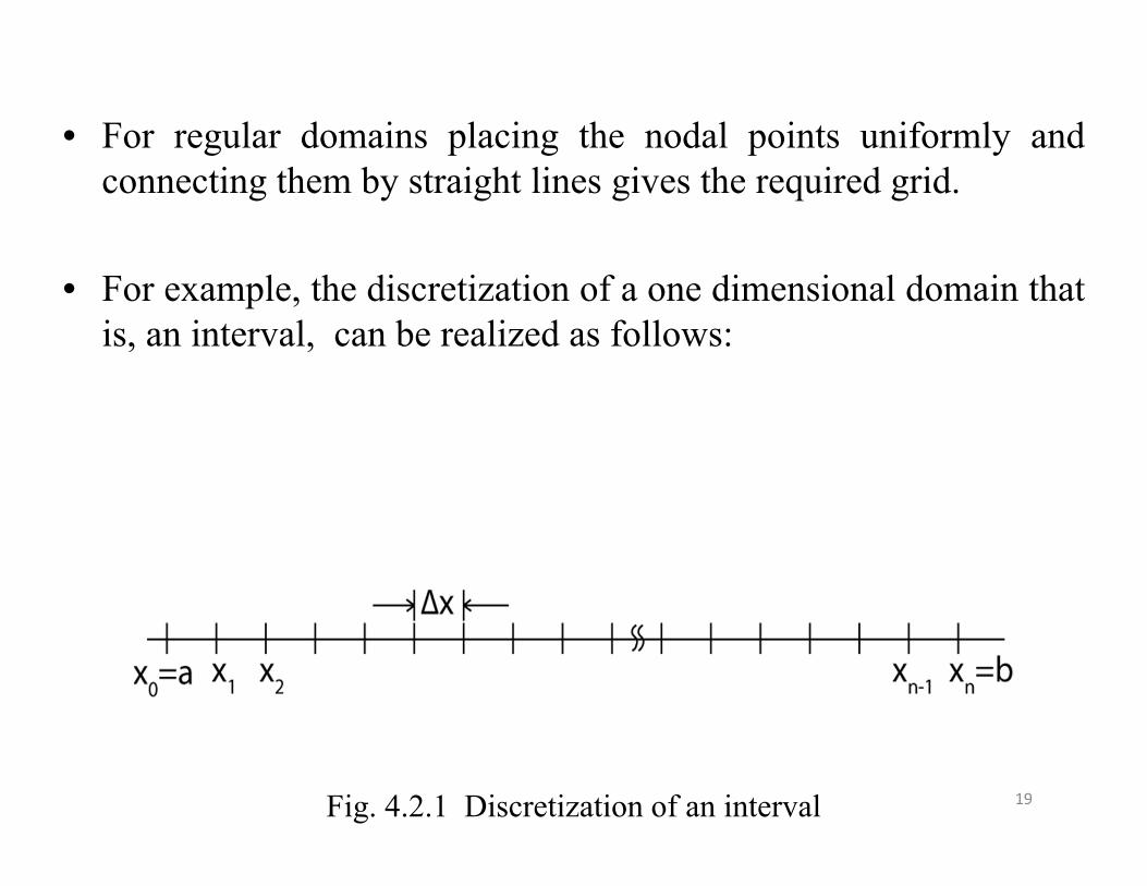
• For regular domains placing the nodal points uniformly andconnecting them by straight lines gives the required grid.

• For example, the discretization of a one dimensional domain thatis, an interval, can be realized as follows:

Fig. 4.2.1 Discretization of an interval 19

• In this discretization, a set of uniformly distributed points x0,x1,….xn are identified such that x0 = a, xn = b and xi – xi-1 = ∆ xfor i = 1,2,…n. where, ∆x is the step length.

• A uniform grid means the distance between any two consecutivepoints xi and xi-1 is constant. Otherwise, the discretization iscalled non-uniform.

• The coordinate of any mesh point is computed using(4.2.1)

• Function value u at any point xi is represented by

* 0,1, 2...x a i x i ni

0,1,2...u x u i ni i

20

• If Ω is a rectangular two-dimension domain bounded by [a,b] x[c,d], then it can be discretized as:

Fig. 4.2.2 Discretization of a rectangular domain

• The coordinates of any point p(xi,yj) are obtained using

(4.2.2)* , 0,1,2,..., , * , 0,1,2,...,0 0x x i x i n y y j y j mi j

21

• Further, the dependent variable u at any point P is representedusing ui,j = u(xi, yj).

• A similar extension can be carried out for higher dimensionaldomains.

• The second step is the discretization of the governing equations.To realize this, there are several methods. In the present lecture,the Taylor series based method is highlighted.

• Consider a function u which depends on the independentvariable x in the interval [a, b].

22

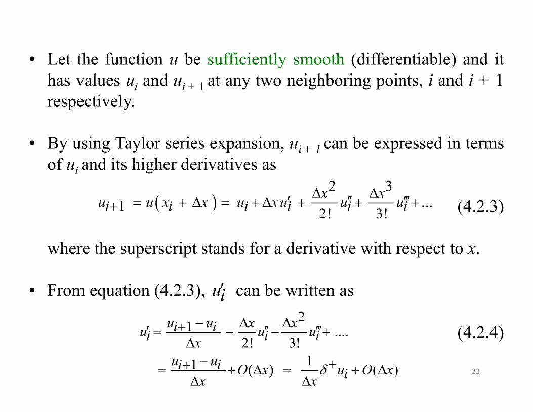
• Let the function u be sufficiently smooth (differentiable) and ithas values ui and ui + 1 at any two neighboring points, i and i + 1respectively.

• By using Taylor series expansion, ui + 1 can be expressed in termsof ui and its higher derivatives as

(4.2.3)

where the superscript stands for a derivative with respect to x.

• From equation (4.2.3), can be written as

(4.2.4)

2 3

...1 2! 3!x xu u x x u xu u ui i i i i i

ui2

1 ....2! 3!

11 ( ) ( )

u u x xi iu u ui i ixu ui i O x u O xix x

23

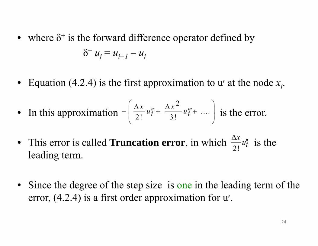
• where δ+ is the forward difference operator defined byδ+ ui = ui+1 – ui

• Equation (4.2.4) is the first approximation to u׳ at the node xi.

• In this approximation is the error.

• This error is called Truncation error, in which is the leading term.

• Since the degree of the step size is one in the leading term of the error, (4.2.4) is a first order approximation for u׳.

2....

2 ! 3 !x xu ui i

2!x ui

24

• The order of approximation is an important concept in theprocess of discretization which gives an immediate insight aboutwhat kind of accuracy can be expected from the scheme.

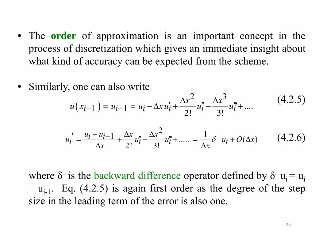
• Similarly, one can also write(4.2.5)

(4.2.6)

where δ- is the backward difference operator defined by δ- ui = ui– ui-1. Eq. (4.2.5) is again first order as the degree of the stepsize in the leading term of the error is also one.

2 3

....1 1 2! 3!x xu x u u xu u ui i i i i i

2 1' 1 ..... ( )2! 3!

u u x xi iu u u u O xi i i ix x

25

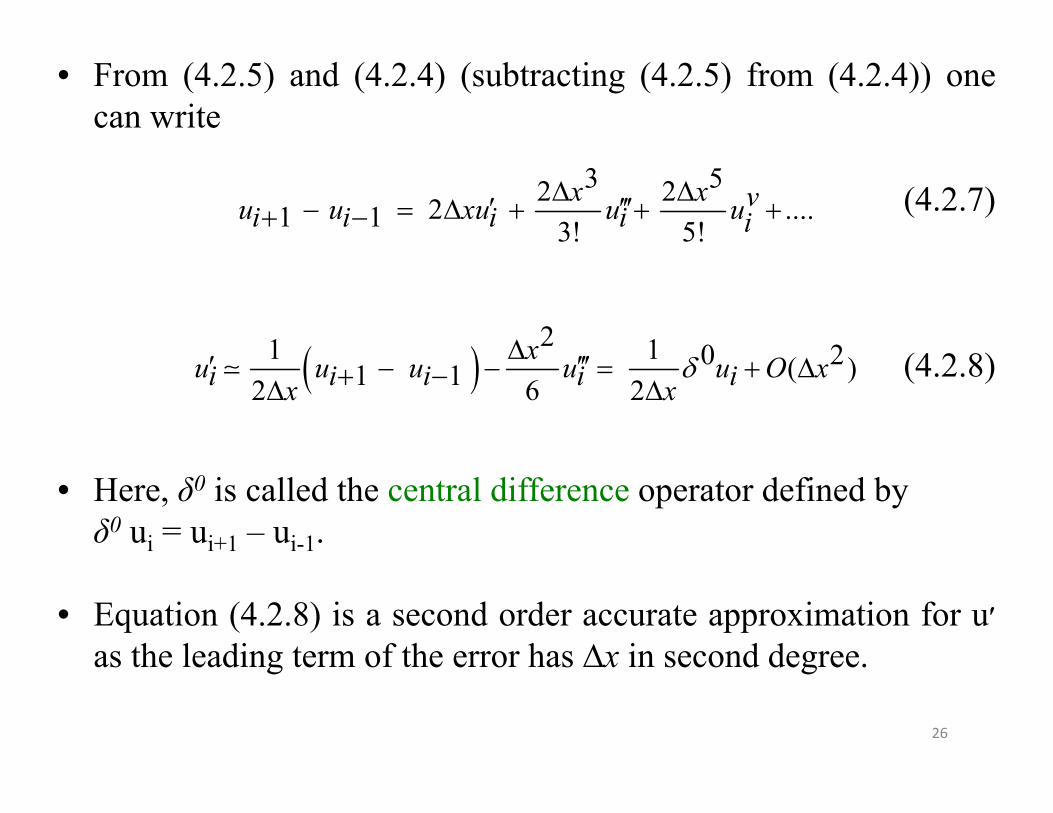
• From (4.2.5) and (4.2.4) (subtracting (4.2.5) from (4.2.4)) onecan write

(4.2.7)

(4.2.8)

• Here, δ0 is called the central difference operator defined byδ0 ui = ui+1 – ui-1.

• Equation (4.2.8) is a second order accurate approximation for u׳as the leading term of the error has ∆x in second degree.

3 52 ....1 1 3! 5!

x x vu u xu u ui i i i i

21 1 0 2( )1 1 6xu u u u u O xi i i i ix x

26

• Alternatively, adding (4.2.4) and (4.2.5) gives

(4.2.9)

(4.2.10)

• where δ2 is the central difference operator for second derivativewhich is a second order accurate approximation.

2 42 ....1 1 2! 4!

x x ivu u u u ui i i i i

22 21 1

2 22 1 ( )

12ivi i i

i i iu u u xu u u O x

x x

27

Numerical Implementation

• The finite difference approximations (4.2.4), (4.2.6), (4.2.8), and(4.2.10) can be used to replace the first and second orderderivative terms of a differential equation to convert it into adifference (possibly linear algebraic) equation at every nodalpoint of the interior of the domain.

• Note that the central approximation (4.2.8) is one order betteraccurate than the forward (4.2.4) and backward (4.2.6)approximations.

• To understand the implementation, consider the followingboundary value problem (BVP).

(4.2.11)2 2 2 sin(ln ) 0, 1 2, (1) 1and (2) 22 2d u du u x x u u

x dxdx x

28

• The analytical solution of the BVP Eq. (4.2.11) is

(4.2.12)

• The finite difference solution of Eq. (4.2.11) is obtained byreplacing its first and second order derivative terms of with(4.2.7) and (4.2.8), respectively to get

(4.2.13)

• Note that at node numbers ‘0’ and ‘n’, we have boundaryconditions and the given differential equation may not be valid atthese points, therefore, at these nodes we have (from theboundary conditions)

u0 = 1.0 and un = 2.0 (4.2.14)

2.03831( ) 1.10869 3sin log( ) 5cos log2 34xu x x x x

x

2 2 21 1 1 1 2( ) sin log( ) 02 2

for 1,2,..., 1

u u u u ui i i i i O x u xi ix xix xii n

29

• Equation (4.2.13) has n-1 equations in n+1 variables, thereforeadding Eq. (4.2.14) closes the system to solve for the unknownsui, for i = 1, 2, . . . , n-1.

• Rearranging the terms in (4.2.13) gives

(4.2.15)

• Equation (4.2.15) is a linear system with tri-diagonal coefficientmatrix. Solving such linear algebraic systems is the third andfinal step of the numerical schemes.

1 1 2 2 1 1 sin log( )1 12 2 2 2( )

1,2,... 1

u u u xi i i ix x x xi ix x x xii n

30

• After solving Eq. (4.2.15) with step lengths (∆x) 1/40, 1/80 and1/160, the absolute errors in the numerical solution are computedand compared in the Fig. 4.2.3

Fig. 4.2.3 Comparison absolute errors with three distinct discretizations31

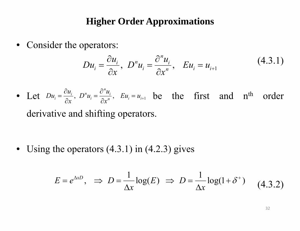
Higher Order Approximations

• Consider the operators:(4.3.1)

• Let be the first and nth order

derivative and shifting operators.

• Using the operators (4.3.1) in (4.2.3) gives

(4.3.2)

1, ,n

ni ii i i in

u uDu D u Eu ux x

1 1, log( ) log(1 )xDE e D E Dx x

1, ,n

ni ii i i in

u uDu D u Eu ux x

32

• Expanding the log function gives

(4.3.3)

• Similar replacements of E with backward difference operator δ-

or central difference operator δ gives

(4.3.4)

(4.3.5)

where

2 3 41 ( ) ( ) ( ) ...2 3 4i iDu u

x

2 3 41 ( ) ( ) ( ) ...2 3 4i iDu u

x

3 51 ...24 640i iDu u

x

1/ 2 1/ 2i i iu u u

33

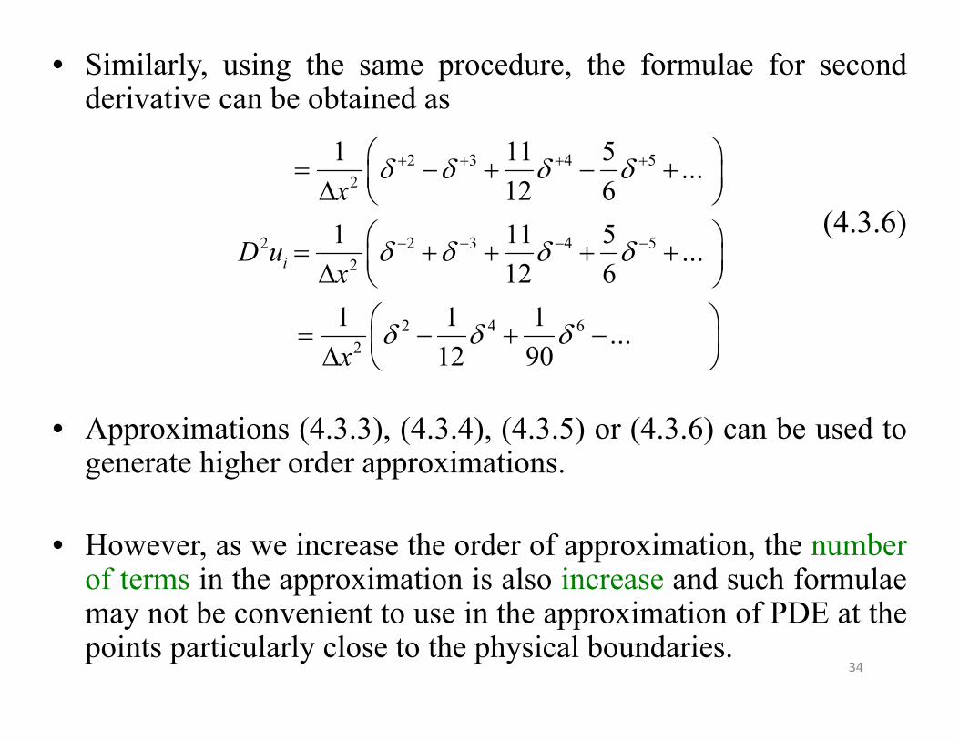
• Similarly, using the same procedure, the formulae for secondderivative can be obtained as

(4.3.6)

• Approximations (4.3.3), (4.3.4), (4.3.5) or (4.3.6) can be used togenerate higher order approximations.

• However, as we increase the order of approximation, the numberof terms in the approximation is also increase and such formulaemay not be convenient to use in the approximation of PDE at thepoints particularly close to the physical boundaries.

2 3 4 52

2 2 3 4 52

2 4 62

1 11 5 ...12 6

1 11 5 ...12 6

1 1 1 ...12 90

i

x

D ux

x

34

Numerical Illustration• The central difference approximation in (4.3.6) may be used

until second term to generate a fourth order approximate formulafor the Poisson equation (in two–dimensions)

• Potential flow equations, discussed in Module 2 have a similarform.

• Consider the required fourth order approximations of the secondderivatives in x and y directions, respectively, at any typicalnodal point, say (i, j), as,

2 2

2 2 ( , )u u f x yx y

2 22 2 2 2

, ,2 2 2 2

1 1 1 11 and 112 12x x i j y y i j

u uu ux x y y

35

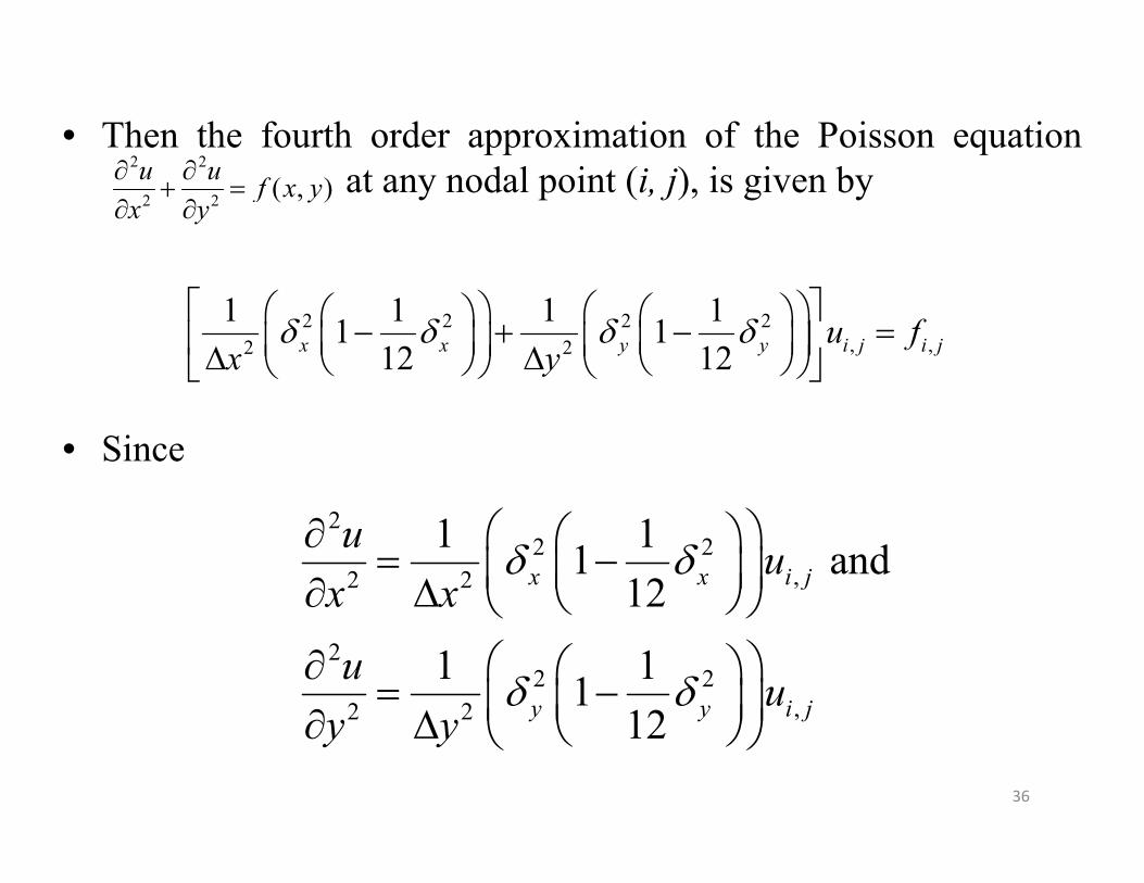
• Then the fourth order approximation of the Poisson equationat any nodal point (i, j), is given by

• Since

22 2

,2 2

22 2

,2 2

1 11 and 12

1 1112

x x i j

y y i j

u ux x

u uy y

2 2

2 2 ( , )u u f x yx y

2 2 2 2, ,2 2

1 1 1 11 112 12x x y y i j i ju f

x y

36

• For the sake of simplicity assume, x = y (the followingprocedure is also valid without this assumption).

• Rewrite the discretized equation as

• Multiplying with gives (after using thecommutative nature of the finite difference operators)

2 2 2 2 2, ,

1 11 112 12x x y y i j i ju x f

1 12 21 11 1

12 12x y

37

1 12 2 2 2

,

1 12 2 2

,

1 11 112 12

1 11 112 12

x y y x i j

x y i j

u

x f

• Expanding the terms on the left hand sideusing

• and neglecting the terms which are having the order more thantwo gives

1 12 21 11 , 1

12 12x y

1 22 2 2

1 22 2 2

1 1 11 1 ...12 12 12

1 1 11 1 ...12 12 12

x x x

y y y

2 2 2 2 2 2 2, ,

1 1 1 11 1 1 112 12 12 12x y y x i j x y i ju x f

38

• Neglecting the product term (since it produces terms at higherorder level) on the right hand side, the final scheme can bewritten as

2 2 2 2 2 2 2 2 2, ,

2 1 1112 12 144x y x y i j x y x y i ju x f

2 2 2 2 2 2 2, ,

2 2 2 2 2 2 2, ,

1 116 12

or

12 12 2 12

x y x y i j x y i j

x y x y i j x y i j

u x f

u x f

39

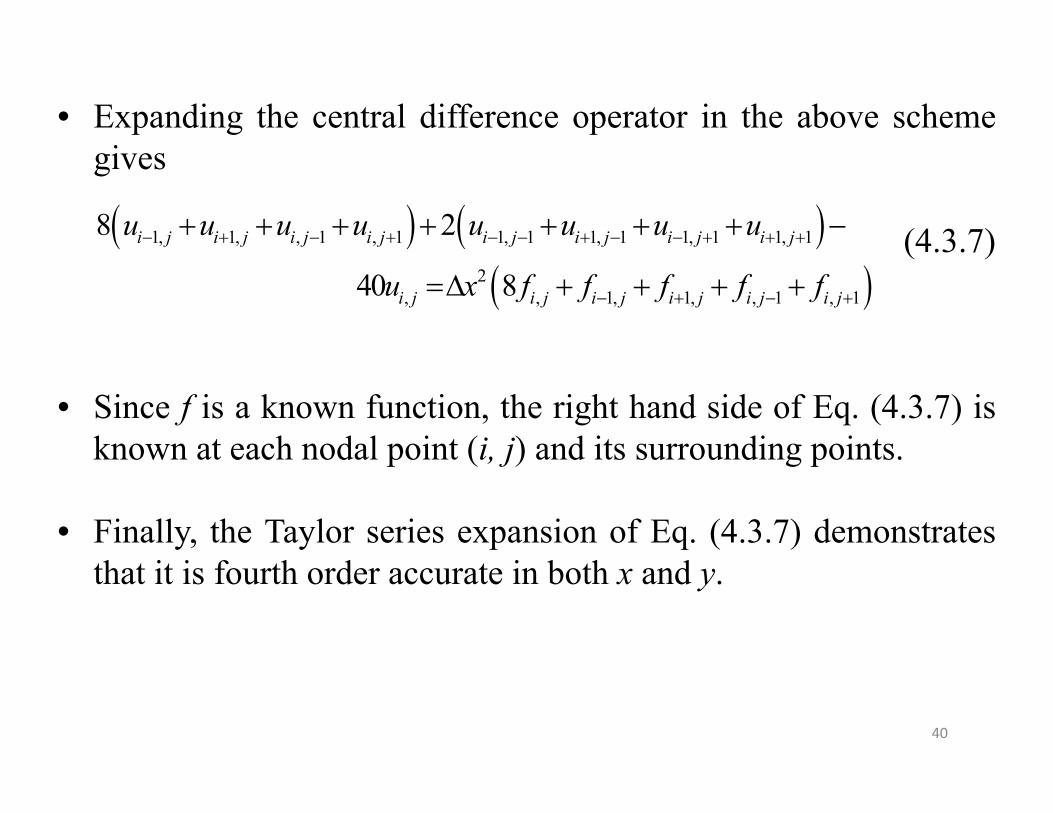
• Expanding the central difference operator in the above schemegives

(4.3.7)

• Since f is a known function, the right hand side of Eq. (4.3.7) isknown at each nodal point (i, j) and its surrounding points.

• Finally, the Taylor series expansion of Eq. (4.3.7) demonstratesthat it is fourth order accurate in both x and y.

1, 1, , 1 , 1 1, 1 1, 1 1, 1 1, 1

2, , 1, 1, , 1 , 1

8 2

40 8

i j i j i j i j i j i j i j i j

i j i j i j i j i j i j

u u u u u u u u

u x f f f f f

40

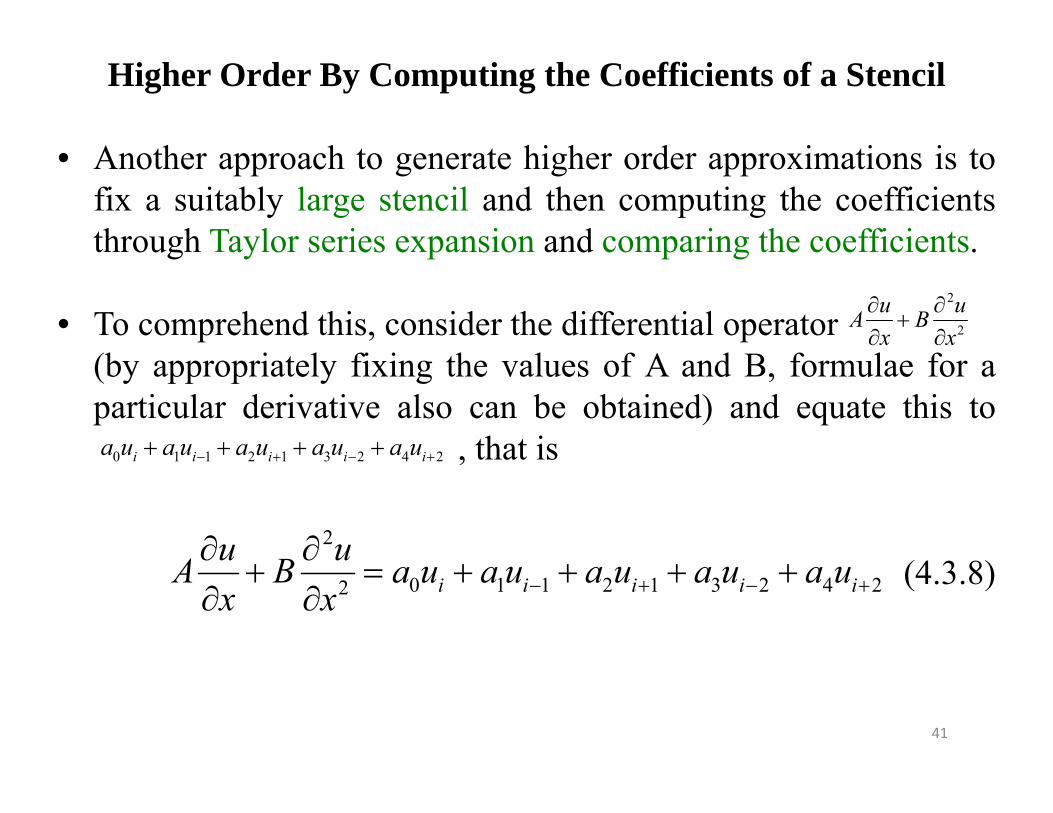
Higher Order By Computing the Coefficients of a Stencil

• Another approach to generate higher order approximations is tofix a suitably large stencil and then computing the coefficientsthrough Taylor series expansion and comparing the coefficients.

• To comprehend this, consider the differential operator(by appropriately fixing the values of A and B, formulae for aparticular derivative also can be obtained) and equate this to

, that is

(4.3.8)

2

2

u uA Bx x

0 1 1 2 1 3 2 4 2i i i i ia u a u a u a u a u

2

0 1 1 2 1 3 2 4 22 i i i i iu uA B a u a u a u a u a ux x

41

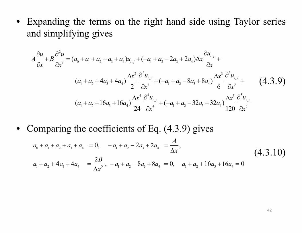
• Expanding the terms on the right hand side using Taylor seriesand simplifying gives

(4.3.9)

• Comparing the coefficients of Eq. (4.3.9) gives

(4.3.10)

2,

0 1 2 3 4 , 1 2 3 42

2 32 3, ,

1 2 3 4 1 2 3 42 3

4 54 5, ,

1 2 3 4 1 2 3 44 5

( ) ( 2 2 )

( 4 4 ) ( 8 8 )2 6

( 16 16 ) ( 32 32 )24 120

i ji j

i j i j

i j i j

uu uA B a a a a a u a a a a xx x x

u ux xa a a a a a a a

x xu ux x

a a a a a a a ax x

0 1 2 3 4 1 2 3 4

1 2 3 4 1 2 3 4 1 2 3 42

2

4 8 16

0, 2 ,

24 , 8 0, 16 0

a a a a a a a a a

a a a a a a a a a a a a

Ax

Bx

42

Finite Difference Schemes for Elliptic Equations

• Consider a two-dimensional Poisson equation given by

(4.4.1)

• First, generate the grid by discretizing the domain Ω with steplengths ∆x and ∆y in x and y directions, respectively (for anexample in a rectangular domain, refer Fig. 4.2.2).

• Then at each grid point of the domain, discretize the given Eq.(4.4.1) by replacing the partial derivatives of the equation withsecond order finite difference approximations (4.2.10) to get

2 22

2 2 ( , ), ( , )xu u f x y x y

y

43

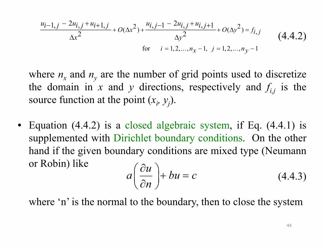
(4.4.2)

where nx and ny are the number of grid points used to discretizethe domain in x and y directions, respectively and fi,j is thesource function at the point (xi, yj).

• Equation (4.4.2) is a closed algebraic system, if Eq. (4.4.1) issupplemented with Dirichlet boundary conditions. On the otherhand if the given boundary conditions are mixed type (Neumannor Robin) like

(4.4.3)

where ‘n’ is the normal to the boundary, then to close the system

2 2( ) ( ) ,

for 1,2,... , 1, 1,2,... , 1

2 21, , 1, , 1 , , 12 2O x O y fi j

i n j nx y

u u u u u ui j i j i j i j i j i j

x y

ua bu cn

44

• The derivative terms in Eq. (4.4.3) are also approximated usingthe first order accurate forward or backward differenceapproximations at every grid point of the boundary, that is, at i =0 or nx or j = 0 or ny.

• Particularly, if the boundary condition Eq. (4.4.3) is given at i =0 or at j = 0 then the forward difference approximation and if itis given at i = nx or at j = ny then backward differenceapproximations maybe used for the discretization.

• Since the forward or backward difference approximations areonly first order accurate, the overall accuracy of the problem isconsidered as first order though the governing equation isapproximated to the second order accuracy.

45

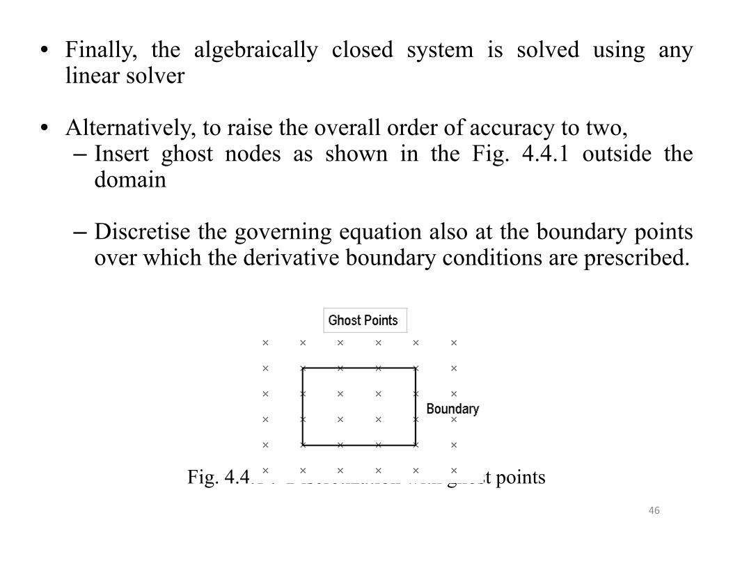
• Finally, the algebraically closed system is solved using anylinear solver

• Alternatively, to raise the overall order of accuracy to two,– Insert ghost nodes as shown in the Fig. 4.4.1 outside the

domain

– Discretise the governing equation also at the boundary pointsover which the derivative boundary conditions are prescribed.

Fig. 4.4.1 : Discretization with ghost points46

• Then eliminate the data points at these ghost points using theequations obtained by approximating the derivative boundaryconditions using second order central difference approximations.

• Solver for (4.4.2) : Due to the sparseness of the coefficientmatrix generated through (4.4.2) (note that only five diagonals ofthis matrix, whatever the size of the system, has non-zeroentries) using any direct method unnecessarily increases thenumber of computations.

• Further, the iterative methods like Jacobi, Gauss Siedel are tooslow in their convergence, therefore, alternatively one can applythe ADI (Alternate Direction Implicit) method which is based online-Gauss Seidel solver.

47

Implementation of the ADI method

• In the first step, on each vertical line , the tri diagonal system

is solved (ny-1 times) using Thomas algorithm (refer Module 5)

• In the second step, on each horizontal line

is solved (nx-1 times) once again using Thomas algorithm

• The procedure is repeated until the convergence after starting theiterative process with iteration number as 0.

,

for 1,2,... , 1

1 1 1 1 11 1 12 ,1, 1, , 1 , 12 2 2 2 2y yfi j

i nx

k k k k ku u u u u yi ji j i j i j i jx x x

,

for 1, 2,... , 1

1 1 1 1 11 1 12 ,, 1 , 1 1, 1,2 2 2 2 2y y y xfi j

j ny

k k k k ku u u u ui ji j i j i j i jx

48

Numerical Illustration

• Consider the two-dimensional heat flow, governed by

(4.4.5)

where is the Laplace operator, in a rectangular duct. The ductsurfaces are considered to be perfectly insulated. The lengths are(x,y) = (4, 3) with boundary conditions and discretization asshown in the Fig. 4.4.2.

• The objective is to find the temperature distribution on thesurface of the sheet.

2 22

2 20u uu

x y

2

49

Figure 4.4.2 Domain and boundary conditions

Solution:

With the discretization of the domain as given in the Fig. 4.4.2,the step lengths are in x and y directions, respectively.2 1,

4 3

50

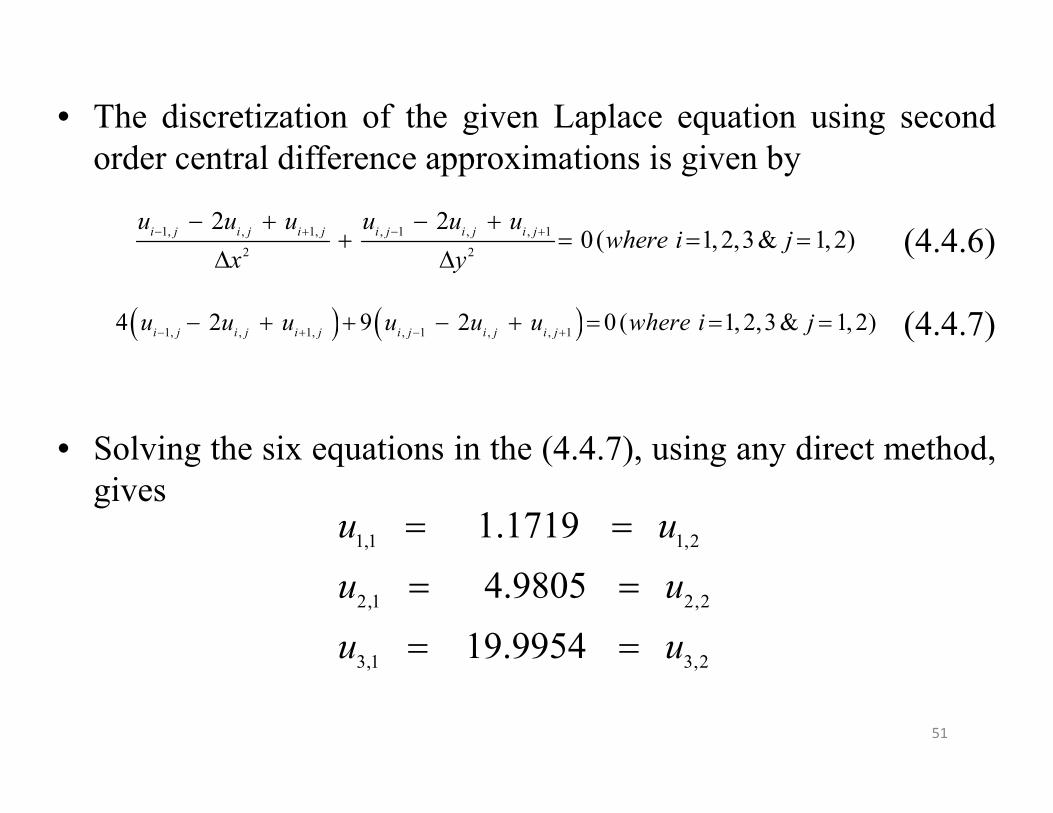
• The discretization of the given Laplace equation using secondorder central difference approximations is given by

(4.4.6)

(4.4.7)

• Solving the six equations in the (4.4.7), using any direct method,gives

1, , 1, , 1 , , 14 2 9 2 0 ( 1, 2,3 & 1, 2)i j i j i j i j i j i ju u u u u u where i j

1,1 1,2

2,1 2,2

3,1 3,2

1.17194.9805

19.9954

u uu uu u

1, , 1, , 1 , , 12 2

2 20( 1, 2,3& 1,2)i j i j i j i j i j i ju u u u u uwhere i j

x y

51

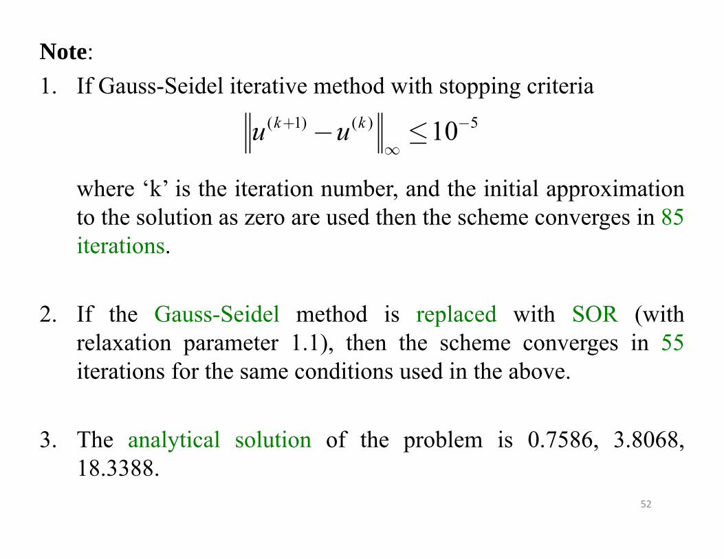
Note:1. If Gauss-Seidel iterative method with stopping criteria

where ‘k’ is the iteration number, and the initial approximationto the solution as zero are used then the scheme converges in 85iterations.

2. If the Gauss-Seidel method is replaced with SOR (withrelaxation parameter 1.1), then the scheme converges in 55iterations for the same conditions used in the above.

3. The analytical solution of the problem is 0.7586, 3.8068,18.3388.

( 1) ( ) 510k ku u+ -

¥- £

52

Note:

4. The percentage errors in the obtained numerical solution are54%, 30%, 9% which are very high.

5. If the step lengths are changed to 2/40 and 1/30 in x and ydirections, respectively then the solution is improved to 0.7620,3.8182, 18.3531 and the percentage errors are then reduced to0.5%, 0.3%, 0.078%.

53

Laplace Equation in Circular Geometries

• Consider the steady diffusion problem over a thin circular platewhich is governed by Laplace equation in polar coordinatesgiven by,

(4.4.8)

where r and θ are radial and angular coordinates.

2 2

2 2 21 1 0 0 , 0 2a

u u u r rr r r r

54

• If Dirichlet conditions are given at r = 0 and ra, and periodicconditions are used in angular direction then the second ordercentral difference approximation of (4.38) gives

(4.4.9)

where dr and dθ are step lengths in radial and angulardirections, respectively.

• Varying i and j in Eq. (4.4.9) gives a linear system which can besolved for the solution of Eq. (4.4.8).

1, , 1, 1, 1, , 1 , , 12 2 21 1 12 2 0i j i j i j i j i j i j i j i j

i i

u u u u u u u udr r dr r d

55

• In the absence of any boundary condition at r = 0, discretizationof Eq. (4.4.8) in the conventional way leads to one over zero insecond and third terms of Eq. (4.4.9). In such cases, u at r = 0 isobtained using

(4.4.10)

• To obtain Eq. (4.4.10), discretize the Cartesian equivalent of Eq.(4.4.8) at the center of the circle with radius ra and take the meanafter repeating the same on the (nθ+1 times) rotated stencil.

00

11

a

n

ii r r

u un

56

Difference Schemes for Parabolic Equations

One-dimensional problems:

• Consider the unsteady diffusion problem (parabolic in nature) ina thin wire governed by the differential equation

(4.5.1)

• Assume that the initial conditions, the distribution of u at t = 0and the boundary conditions, u at x = a and b are given.

2

2 , ( , ), 0u uk x a b tt x

57

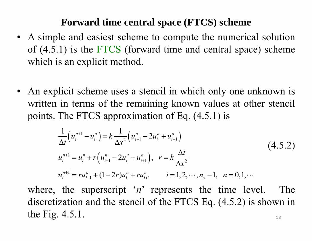
Forward time central space (FTCS) scheme• A simple and easiest scheme to compute the numerical solution

of (4.5.1) is the FTCS (forward time and central space) schemewhich is an explicit method.

• An explicit scheme uses a stencil in which only one unknown iswritten in terms of the remaining known values at other stencilpoints. The FTCS approximation of Eq. (4.5.1) is

(4.5.2)

where, the superscript ‘n’ represents the time level. Thediscretization and the stencil of the FTCS Eq. (4.5.2) is shown inthe Fig. 4.5.1.

11 12

11 1 2

11 1

1 1 2

2 ,

(1 2 ) 1, 2, , 1, 0,1,

n n n n ni i i i i

n n n n ni i i i i

n n n ni i i i x

u u k u u ut x

tu u r u u u r kx

u ru r u ru i n n

58

Fig. 4.5.1 Discretization and the stencil of FTCS scheme

• In the Fig. 4.5.1, there is only one stencil point at n+1th timelevel which is the unknown and three points at nth time levelwhich anyway are known.

• Therefore using Eq. (4.5.2), one unknown at a time at n+1 timelevel can be computed by varying i = 1, 2, . . ., nx-1.

59

• Taylor series expansion of Eq. (4.5.2) demonstrates that theFTCS scheme is first order accurate in time and second order inspace.

Backward time central space (BTCS) scheme

• The BTCS approximation of Eq. (4.5.1) gives

(4.5.3)

• Equation (4.5.3) is an implicit scheme which has more than oneunknown at nth time level, therefore one equation alone can’t besolved unless it is clubbed with more number of equations toclose the system.

11 12

11 1 2

1 1 2

(1 2 ) , , 1,2, , 1, 1,2,

n n n n ni i i i i

n n n ni i i i x

u u k u u ut x

tru r u ru u r k i n nx

60

• This is done by grouping all the discretized equations at aparticular time level and solving them in one step using say,Thomas algorithm if the resultant system is a tri-diagonal one.

• The same is repeated by incrementing the value of ‘n’ until therequired time level is reached.

• This type of procedure is called a time marching scheme.

61

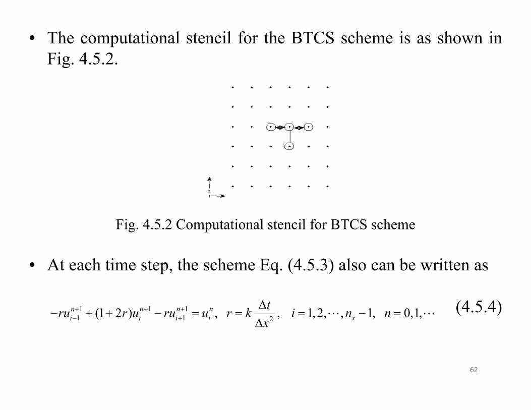
• The computational stencil for the BTCS scheme is as shown inFig. 4.5.2.

Fig

Fig. 4.5.2 Computational stencil for BTCS scheme

• At each time step, the scheme Eq. (4.5.3) also can be written as

(4.5.4)1 1 11 1 2(1 2 ) , , 1, 2, , 1, 0,1,n n n n

i i i i xtru r u ru u r k i n nx

62

Weighted average scheme• Weighted average of Eqs. (4.5.1) and (4.5.3), gives

(4.5.4)

• For θ equals to 0 and 1, Eq. (4.5.4) gives FTCS and BTCSschemes, respectively. The Taylor series expansion of (4.5.4)gives

(4.5.4)

• Therefore, weighted average scheme Eq. (4.5.4) is second orderaccurate in space and first order in time if . The scheme isalso second order accurate in time if . The weighted averagescheme with is known as Crank-Nicolson scheme.

1 1 1 11 1 1 12

1 1 11 1 1 1

2

1 (1 ) 2 2

(1 2 ) (1 ) (1 2(1 ) ) (1 )

, 0 1, 1,2, , , 0,1,

n n n n n n n ni i i i i i i i

n n n n n ni i i i i i

x

ku u u u u u u ut xr u r u r u r u r u r u

tr k i n nx

2 2 2 3 2 4 2 2 4

2 2 3 4 2 212 2 12 2

n n n ni i i iu u u t u k x u k t x uk t

t x t t x t x

12

12

12

63

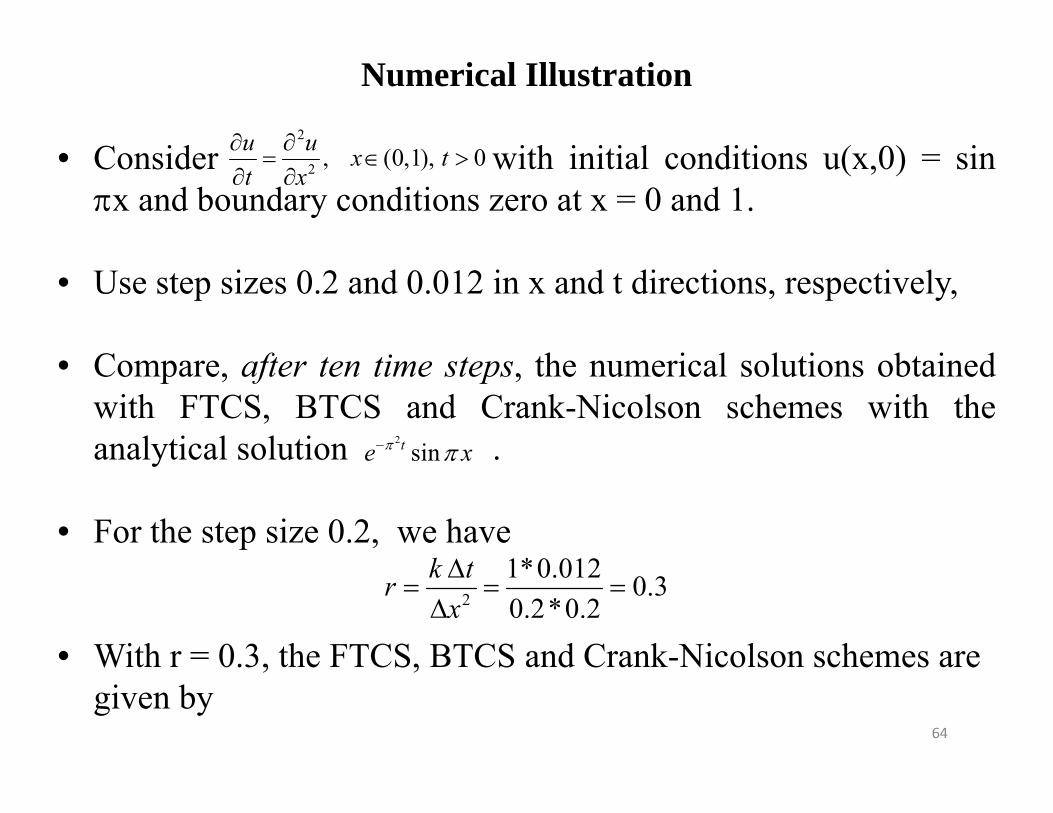
Numerical Illustration

• Consider with initial conditions u(x,0) = sinx and boundary conditions zero at x = 0 and 1.

• Use step sizes 0.2 and 0.012 in x and t directions, respectively,

• Compare, after ten time steps, the numerical solutions obtainedwith FTCS, BTCS and Crank-Nicolson schemes with theanalytical solution .

• For the step size 0.2, we have

• With r = 0.3, the FTCS, BTCS and Crank-Nicolson schemes are given by

2

2 , (0,1), 0u u x tt x

2

sinte x

2

1*0.012 0.30.2*0.2

k trx

64

(4.5.6)

• Equation (4.5.6) depends only on the value of r and isindependent of the step sizes.

• The solution and the percentage errors generated by the threeschemes (FTCS, BTCS and Crank_Nicolson), after marching 10times in the time direction using Eq. (4.5.6), are compared in theTable 4.5.1.

11 1

1 1 11 1

1 1 11 1 1 1

0.3 0.4 0.3

0.3 1.6 0.3

0.15 1.3 0.15 0.15 0.7 0.15for 1, 2,3, 4, 0,1, 2, ,9

n n n ni i i i

n n n ni i i in n n n n ni i i i i i

u u u u

u u u u

u u u u u ui n

65

Table 4.5.1 Comparison of the analytical and numerical solutions and their errors

• The initial and boundary conditions in the above computationsare taken from the exact solution.

X AnalyticalFTCS BTCS Crank-Nicolson

Solution Error Solution Error Solution Error

0.2 0.1798 0.1740 3.22% 0.1986 10.46% 0.1866 3.79%

0.4 0.2910 0.2816 3.22% 0.3214 10.46% 0.3020 3.79%

66

Two-dimensional problems• Consider the unsteady diffusion over a flat plate governed by the

differential equation(4.5.7)

Assume that the initial and boundary conditions on u are known.

Explicit scheme• Approximating the time derivative with forward difference and

space derivatives with central differences gives a scheme

(4.5.8)

2 2

2 2 , ( , ) ( , ) ( , ), 0u u uk x y a b X c d tt x y

1, , 1, , 1, , 1 , , 12 2

1, , 1 1, , 1, 2 , 1 , , 1

1 22 2

1, 2 , 1 1 1, 1 2

1 1 12 2

2 2

,

(1 2 2 )

n n n n n n n ni j i j i j i j i j i j i j i j

n n n n n n n ni j i j i j i j i j i j i j i j

n n ni j i j i j i

u u k u u u u u ut x y

u u r u u u r u u u

t tr k r kx y

u r u ru r r u

, 1 1, 2 , 1

1,2, , 1, 1,2, , 1, 0,1,

n n nj i j i j

x y

ru r u

i n j n n

67

• Here, ∆y is the step length in y direction. Taylor seriesexpansion of Eq. (4.5.8) shows that the explicit scheme is firstorder accurate in time and second order in space (both in x and ydirections).

• Weighted average or Crank-Nicolson type of approximation to(4.5.7) gives a penta-diagonal system like Eq. (4.4.2) at the n+1th

time level, solving such a system is very expensivecomputationally, therefore, alternatively ADI method can bedeveloped as follows:

(4.5.9)

1 1 1 12 2 2 2

, , 1, , 1, , 1 , , 12 2

1 1 1 11 1 1 12 2 2 2

, , 1, , 1, , 1 , , 12 2

2 2/ 2

2 2/ 2

n n n nn n n ni j i j i j i j i j i j i j i j

n n n nn n n ni j i j i j i j i j i j i j i j

u u u u u u u uk

t x y

u u u u u u u uk

t x y

68

• First on j is constant lines, using the first tri-diagonal part of Eq.(4.5.9), solution at n+1/2 time level is obtained.

• In the second step, using the solution at the n+1/2 time level overthe i is constant lines and using second tri-diagonal part of Eq.(4.5.9), the solution is marched to the n+1 time level.

• Therefore, for each time level, Eq. (4.5.9) gives (nx-1 + ny-1) tri-diagonal systems in x and y directions which are mush easier tosolve using Thomas algorithm than the penta-diagonal system(of size L X L, where L = (nx-1) * (ny-1)) appears in theweighted average or Crank-Nicolson schemes for twodimensional problems.

69

Convergence

• Here, convergence means, the convergence of the numericalsolution to the analytical solution

• For parabolic and also for all time dependent problems, theconvergence of the numerical solution to the correspondinganalytical solution is carried out through the testing forconsistency and stability since, according to Lax equivalencetheorem,

• Consistency and stability are necessary and sufficient conditionsfor convergence of the finite difference solutions of any timedependent problem.

70

Consistency of a Numerical Scheme

• Under the limiting case of step lengths tending to zero, if a finitedifference scheme converge to the corresponding differentialequation then such a scheme is called consistent.

• Mathematically, it is tested by looking at the truncation error ofthe scheme as the step lengths tend to zero.

• If the truncation error tends to zero as the step lengths tend zerothen the numerical scheme is said to be consistent.

71

Numerical Illustration

• Consider the Taylor series expansion Eq. (4.5.5) of the Weightedaverage scheme Eq. (4.5.4)

given by

• Taking step lengths ∆x and ∆t tending to zero, the series

expansion converges to the governing equation ,

therefore, the weighted average scheme is consistent.

1 1 11 1 1 1(1 2 ) (1 ) (1 2(1 ) ) (1 )n n n n n ni i i i i ir u r u ru ru r u ru

2 2 2 3 2 4 2 2 4

2 2 3 4 2 212 2 12 2

n n n ni i i iu u u t u k x u k t x uk t

t x t t x t x

2

2u ukt x

72

Stability of a Numerical Scheme

• Stability of a numerical scheme deals with the growth of therounding errors during the time marching process.

• Let us illustrate, the stability through the following observation

• Repeat the computations of Eq. (4.5.6) once again with timesteps 0.018 and 0.022 (that is, for the value of r as 0.45 and0.55, respectively) for FTCS and Crank-Nicolson (CN) schemes

• The corresponding solution with r = .45 and .55 are presented inTables 4.5.2 and 4.5.3, respectively

73

Table 4.5.2 Comparison of the solution and errors with r = 0.45.

Table 4.5.3 Comparison of the solution and errors with r = 0.55.

X AnalyticalFTCS Crank-Nicolson

Solution Error Solution Error

0.2 0.3040 0.3045 0.17% 0.3070 1.00%

0.4 0.4954 0.4947 0.14% 0.5016 1.26%

X AnalyticalFTCS Crank-Nicolson

Solution Error Solution Error

0.2 0.2762 0.2301 16.35% 0.2794 1.17%

0.4 0.4484 0.3700 17.49% 0.4542 1.30%

74

• Its clear from the Tables 4.5.2 and 4.5.3 that, with r = 0.45, the FTCSscheme produces solutions with errors less than .2% and CN schemewith errors less than 1.3%.

• However, if the value of r is increased to 0.55, the CN schemecontinues to give solutions with similar errors while the errors inFTCS scheme increased by many folds.

• The behavior of increasing errors with FTCS becomes worse andcompletely dominated by these errors if we still continue thecomputations for higher time levels.

• This is due to the instable nature of the FTCS scheme when the valueof r is greater than 0.5. Mathematically this can be understood usingthe following analysis:

75

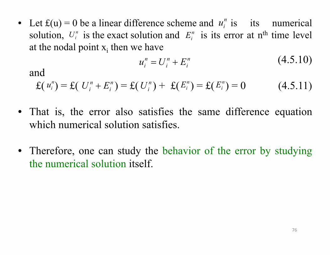
• Let £(u) = 0 be a linear difference scheme and is its numericalsolution, is the exact solution and is its error at nth time levelat the nodal point xi then we have

(4.5.10)and

£( ) = £( ) = £( ) + £( ) = £( ) = 0 (4.5.11)

• That is, the error also satisfies the same difference equationwhich numerical solution satisfies.

• Therefore, one can study the behavior of the error by studyingthe numerical solution itself.

niu

niU n

iE

n n ni i iu U E

niu n n

i iU E niU

niE

niE

76

• Further, if the numerical solution is assumed to be periodic,achieved by reflecting the solution in the region (0, L) in to (-L,L) and expressible in terms of finite Fourier series (since thedomain is of finite length which is discretized with finite steplength) then it can be written as

(4.5.12)

whereN is the number of points in the discretization, (N=L/∆x)

is the amplitude of the jth harmonic,kj is the wave number is the phase angle given by kj ∆x.

j i jN N N

Ik x Ik i xn n n n Iii j j j

j N j N j N

u K e K e K e

njK

1I

77

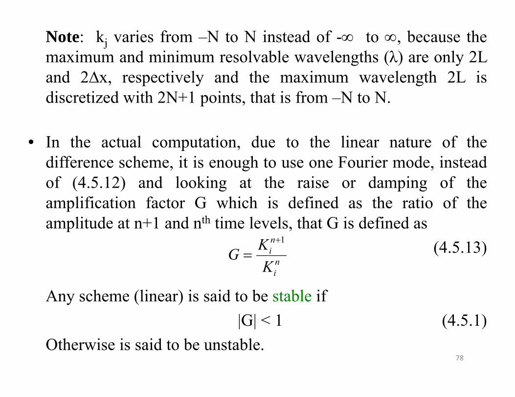
Note: kj varies from –N to N instead of - to , because themaximum and minimum resolvable wavelengths (λ) are only 2Land 2∆x, respectively and the maximum wavelength 2L isdiscretized with 2N+1 points, that is from –N to N.

• In the actual computation, due to the linear nature of thedifference scheme, it is enough to use one Fourier mode, insteadof (4.5.12) and looking at the raise or damping of theamplification factor G which is defined as the ratio of theamplitude at n+1 and nth time levels, that G is defined as

(4.5.13)

Any scheme (linear) is said to be stable if|G| < 1 (4.5.1)

Otherwise is said to be unstable.

1nini

KGK

78

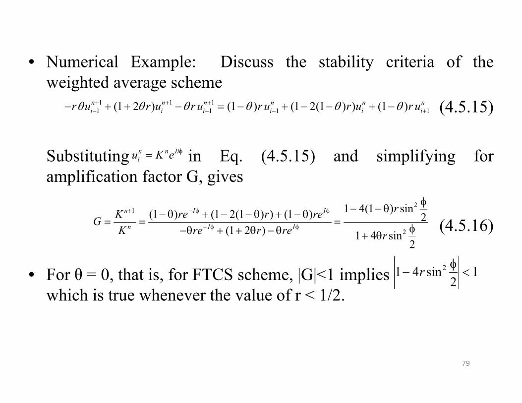
• Numerical Example: Discuss the stability criteria of theweighted average scheme

(4.5.15)

Substituting in Eq. (4.5.15) and simplifying foramplification factor G, gives

(4.5.16)

• For θ = 0, that is, for FTCS scheme, |G|<1 implieswhich is true whenever the value of r < 1/2.

1 1 11 1 1 1(1 2 ) (1 ) (1 2(1 ) ) (1 )n n n n n n

i i i i i ir u r u r u r u r u r u

n n Iiiu K e

21

2

1 4(1 ) sin(1 ) (1 2(1 ) ) (1 ) 2(1 2 ) 1 4 sin

2

n I I

n I I

rK re r reGK re r re r

21 4 sin 12

r

79

• Therefore, FTCS scheme is only conditionally stable. However,for θ greater or equal to ½, Eq. (4.5.16) is unconditionally stable.

• Once again looking at the Tables 4.5.2 and 4.5.3, it is clear thatfor r = 0.45, FTCS scheme is able to produce accurate solutionsbut the round of errors are dominated when the value of r israised to 0.55 because FTCS scheme is not stable at r = 0.55.

• On the other hand due its stable nature of CN scheme for allvalues of r, the round of errors are under control at both r = 0.45and 0.55.

80

Difference schemes for hyperbolic equations

• Consider the one dimensional wave equation

(4.6.1)

where c is a positive constant.

• Equation (4.6.1) requires two initial conditions at t=0u(x,0) = f(x), ut(x,0) = g(x) (4.6.2)

and two boundary conditions at x=0 and L given byu(0,t) = u(L,t) = 0 (4.6.3)

2 22

2 2 , (0, ), 0u uc x L tt x

81

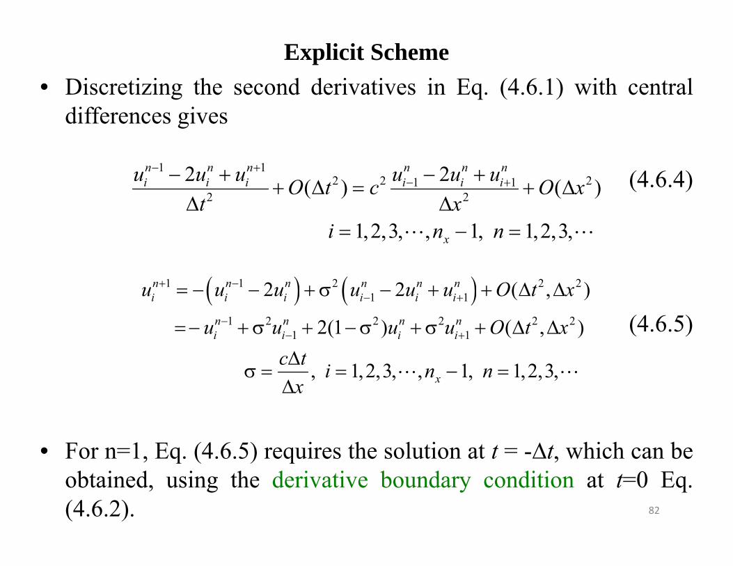
Explicit Scheme• Discretizing the second derivatives in Eq. (4.6.1) with central

differences gives

(4.6.4)

(4.6.5)

• For n=1, Eq. (4.6.5) requires the solution at t = -∆t, which can beobtained, using the derivative boundary condition at t=0 Eq.(4.6.2).

1 12 2 21 1

2 22 2( ) ( )

1,2,3, , 1, 1,2,3,

n n n n n ni i i i i i

x

u u u u u uO t c O xt x

i n n

1 1 2 2 21 1

1 2 2 2 2 21 1

2 2 ( , )

2(1 ) ( , )

, 1,2,3, , 1, 1,2,3,

n n n n n ni i i i i i

n n n ni i i i

x

u u u u u u O t x

u u u u O t xc t i n nx

82

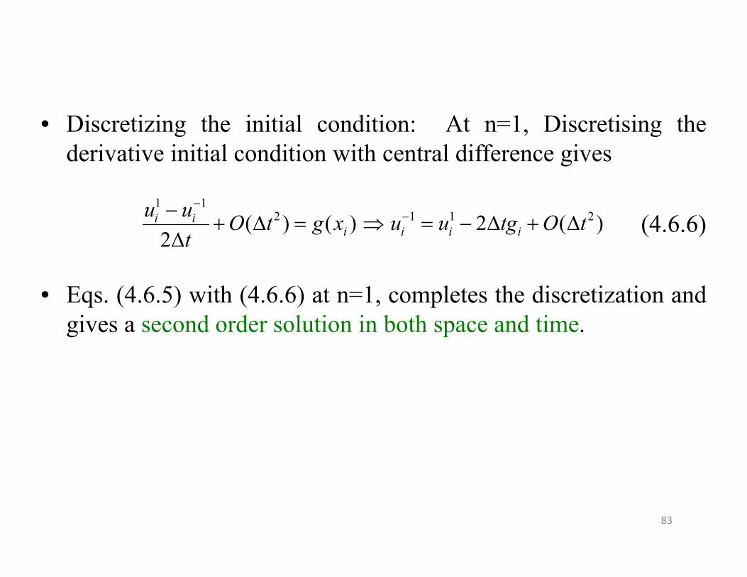
• Discretizing the initial condition: At n=1, Discretising thederivative initial condition with central difference gives

(4.6.6)

• Eqs. (4.6.5) with (4.6.6) at n=1, completes the discretization andgives a second order solution in both space and time.

1 12 1 1 2( ) ( ) 2 ( )

2i i

i i i iu u O t g x u u tg O t

t

83

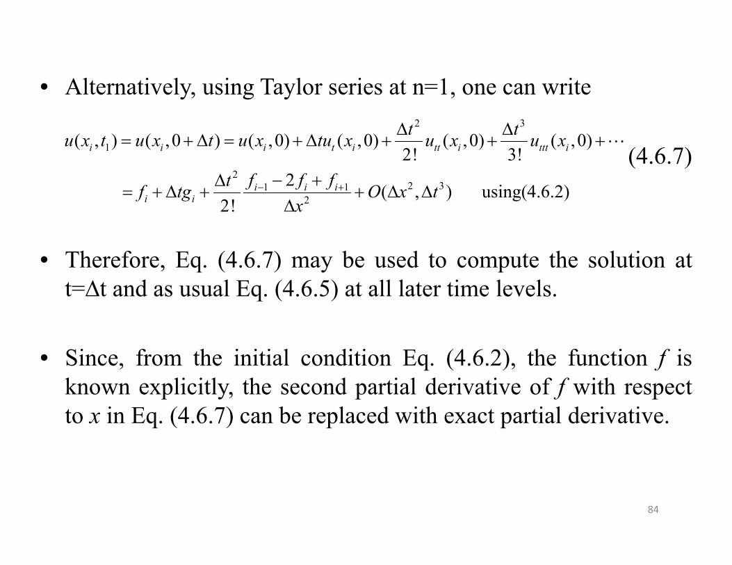
• Alternatively, using Taylor series at n=1, one can write

(4.6.7)

• Therefore, Eq. (4.6.7) may be used to compute the solution att=∆t and as usual Eq. (4.6.5) at all later time levels.

• Since, from the initial condition Eq. (4.6.2), the function f isknown explicitly, the second partial derivative of f with respectto x in Eq. (4.6.7) can be replaced with exact partial derivative.

2 3

1

22 31 1

2

( , ) ( ,0 ) ( ,0) ( ,0) ( ,0) ( ,0)2! 3!

2 ( , ) using(4.6.2)2!

i i i t i tt i ttt i

i i ii i

t tu x t u x t u x tu x u x u x

f f ftf tg O x tx

84

Consistency and Stability of Eq. (4.6.7)

• Taylor series expansion of Eq. (4.6.5) gives

(4.6.8)

• Equation (4.6.5) converges to the governing Eq. (4.6.3) if thestep lengths ∆x, ∆t tending zero, therefore the scheme Eq. (4.6.5)is consistent.

• Equation (4.6.8) also indicates that the scheme Eq. (4.6.5) issecond order in both t and x.

2 2 4 42 2 2 2 4 4

2 2 4 41 ( , )

12u u u uc t c x O t xt x t x

85

• For verifying stability, in Eq. (4.6.5) and simplify to get

• Dividing with gives

(4.6.9)

• Computing K from Eq. (4.6.9) gives,

, provided 1 > A2 (4.6.10)

n n Iiiu K e

1 1 2 ( 1) 2 ( ) 2 ( 1)2(1 )n Ii n Ii n I i n I i n I iK e K e K e K e K e

n IiK e

1 2 ( 1) 2 2 (1) 1 2 2

2 2 2 2

2 2 2 2 2 2

2(1 ) 2cos 2(1 )

2(1 2sin ) 2(1 ) 1 02

2 1 2 sin 1 0 2 1 0 with 1 2 sin2 2

I n IK K e K e K

K K

K K K AK A

2 21 1K A A A i A

86

• Equation (4.6.10) guarantees |K|=1 which is better than |K|>1because in the former, at least the error only grows in accordancewith the solution instead of blowing up in the later situation.However, Eq. (4.6.10) is valid only when

(4.6.11)

Finally, Eq. (4.6.11) is true whenever(4.6.12)

• Equation (4.6.12) is the required condition for the explicitscheme Eq. (4.6.5), to the wave Eq. (4.6.3), to be stable.

2 2 2 2 21 1 1 1 1 2 sin 1 sin 12 2

A A

1c tx

87

CFL ( Courant – Friedrichs – Lewy ) Condition

• It was stated during the classification of the PDE that, thehyperbolic equations have a domain of dependence.

• To illustrate this, consider the D’Alembert’s solution of the waveEq. (4.6.3)-(4.6.4), with x (-,), given by

(4.6.13)

• Equation (4.6.13) demonstrates that the solution of the waveequation at any point (x, t) depends only in the triangular regionbounded by the left running characteristic, the right runningcharacteristic and the x-axis.

1 1( , ) ( ) ( ) ( )2 2

x ct

x ct

u x t f x ct f x ct g v dvc

88

• Therefore, any numerical scheme which is developed to solveEq. (4.6.3) should also use all the data from this region.

• The condition which guarantees such a criteria is called CFLcondition.

• Since, Eq. (4.6.13) uses f and g in the region (xi-atn, xi+atn) on thex-axis to compute the solution at any given point (xi, tn),therefore, according to CFL condition (the numerical domain ofdependence should bound the analytical domain of dependence)that is

(4.6.14) 1

i n i n i ix x ct x n x x c t cc txx

n t

89

• Condition Eq. (4.6.14) is equivalent to the stability condition σ ≤1 for the explicit scheme Eq. (4.6.5).

• Further, if c=1 and the step lengths ∆t=∆x, then from Eq. (4.6.8),the scheme Eq. (4.6.5) is fourth order accurate.

• Therefore, if the step lengths are fixed such that σ = 1, then theexplicit scheme Eq. (4.6.5) gives the best solution (in thisparticular case, that is, for c=1 and ∆t=∆x, the entire right handside of Eq. (4.6.8) becomes zero and Eq. (4.6.5) produces exactsolution).

90

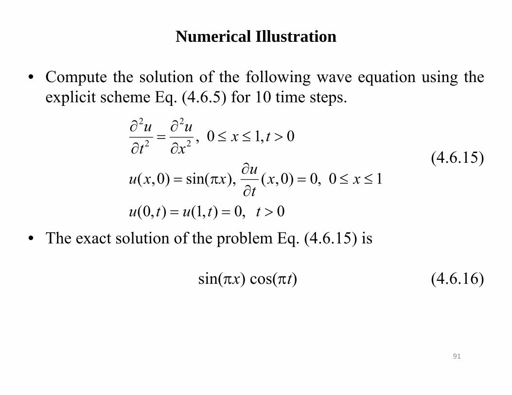
Numerical Illustration

• Compute the solution of the following wave equation using theexplicit scheme Eq. (4.6.5) for 10 time steps.

(4.6.15)

• The exact solution of the problem Eq. (4.6.15) is

sin(x) cos(t) (4.6.16)

2 2

2 2 , 0 1, 0

( ,0) sin( ), ( ,0) 0, 0 1

(0, ) (1, ) 0, 0

u u x tt x

uu x x x xt

u t u t t

91

• Fixing ∆x = 0.1 and ∆t = 0.075 (so that σ = 0.75), scheme Eq.(4.6.5), after 10 time steps (that is at time t = .75), produces the anumerical solution which has been compared with the analyticalsolution in the Table 4.6.1,

• The percentage error is 0.38%.

• The numerical solution in the Table 4.6.1 is generated using theexact solution at the time step ∆t.

• In the computations if ∆t is changed to 0.1 (σ = 1), as discussedearlier, the explicit scheme has produced the exact solution(except for some machine error at 10-15).

92

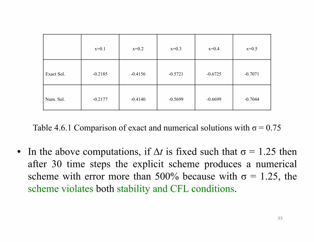
Table 4.6.1 Comparison of exact and numerical solutions with σ = 0.75

• In the above computations, if ∆t is fixed such that σ = 1.25 thenafter 30 time steps the explicit scheme produces a numericalscheme with error more than 500% because with σ = 1.25, thescheme violates both stability and CFL conditions.

x=0.1 x=0.2 x=0.3 x=0.4 x=0.5

Exact Sol. -0.2185 -0.4156 -0.5721 -0.6725 -0.7071

Num. Sol. -0.2177 -0.4140 -0.5699 -0.6699 -0.7044

93